Transducer Thesis

1

CHAPTER 1

INTRODUCTION TO ACOUSTIC SATURATION Acoustic saturation states that as the input voltage to a focused ultrasonic transducer

increases, there exists a limit of the acoustic pressure at the transducer’s focus. The most

significant phenomenon associated with saturation is the presence of nonlinear conditions in the

propagating wave. As the term nonlinear implies, the features of an acoustic waveform change.

For example, at a relatively low applied voltage, the acoustic pressure at a transducer’s focus will

appear sinusoidal, and the positive and negative pressures are approximately equal, as can be

seen in Figure 1.1(a). However, if the input voltage is increased significantly, the positive

pressure at the focus will become larger than the negative pressure at the focus, which can be

seen in Figure 1.1(b). Understanding the origins of the nonlinear characteristics is the basis for

understanding acoustic saturation.

(a) (b) Figure 1.1: Time-domain acoustic waves at the focus for (a) low and (b) high input voltages.

2

1.1 Background There is a need to define some of the terminology that will be used throughout this text.

A system was developed to determine acoustic pressure levels at the focus of an ultrasonic field.

A detailed description of the process is described in Chapter 4, but it is useful to describe some

of the definitions used in that process.

Measurements of a transducer’s ultrasonic pressure characteristics are made in water

because of its availability and well-known characteristics [1]. The basis of the system used to

find the transducer’s focus is the pulse intensity integral (PII) [2]:

PII =1

!" cp t( )#$ %&

2

dt0

T

' (1.1)

where p(t) is the time-domain ultrasonic pressure waveform, ρ is the density of the propagating

medium, c is the speed of sound in the medium, and T is the time interval when the received

pulse at the hydrophone is nonzero [3]. Acoustic pressure waveforms can be collected at various

distances from the transducer, and a series of PII values can be plotted as a function of axial

distance from the transducer, which is shown in Figure 1.2. This is the axial profile for the

transducer. By definition [2], the focus occurs at the maximum point on the derated PII (PII.3)

curve, which is the lower curve shown in Figure 1.2. The .3 subscript comes from the derating

factor 0.3 dB/cm·MHz [2], [3]. The derating factor is an attenuation factor that can be added to

Figure 1.2: Axial profiles for PII and PII.3 versus distance from the transducer.

3

water measurements. The derated pulse intensity integral is defined as [2]:

PII.3 = PII exp !0.069 " fc " z( )#$ %& (1.2)

where fc is the center frequency, z is the distance from the transducer, and 0.069 in the

exponential comes from the conversion:

0.3dB

cm !MHz•Np

8.7dB• 2 = 0.069

Npcm !MHz

The exponential needs to be multiplied by a factor of 2 because PII is an intensity measurement.

Each pressure waveform collected during the measurement process has a peak positive

pressure, or compressional pressure (pc), and a peak negative pressure, or rarefactional pressure

(pr), associated with it. Similar to the PII plots, pc and pr can also be plotted as functions of

distance from the source to obtain pressure profiles for the transducer. The pc and pr values are

also derated by the derating factor and the resulting equations are

pc.3 = pc exp !0.0345 " fc " z( )#$ %&

pr.3 = pr exp !0.0345 " fc " z( )#$ %& (1.3)

where

0.3dB

cm !MHz•Np

8.7dB= 0.0345

Npcm !MHz

and fc and z are the same as before. Axial profiles of pc, pc.3, pr, and pr.3 are shown in Figure 1.3.

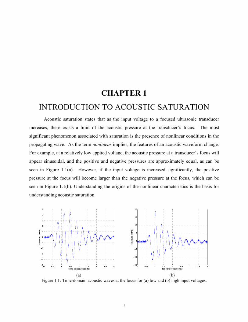
Figure 1.4 shows axial profiles for PII.3, pc.3, and pr.3 normalized to the maximum value

of the PII.3 profile curve. Normalization was done so that all three axial profiles could be plotted

on the same graph. Once the position where PII.3 is a maximum is determined, that position is

then used to determine pc.3 and pr.3, which are the pressure values at the focus. For example, let

the position of the maximum PII.3 for Figure 1.2 be at 2.2 cm. The axial profiles for pc.3 and pr.3

are plotted in Figure 1.3 from 2 to 2.5 cm. The derated acoustic pressures at 2.2 cm would

correspond to the pressures at the focus of the transducer. The pr.3 value can then be used to

determine the mechanical index (MI) at the transducer’s focus. Mechanical index is defined as

[2]:

MI =pr.3

fc (1.4)

The regulatory limit set by the Food and Drug Administration (FDA) is an MI of 1.9 [4].

4

Figure 1.3: Axial profiles for pc and pr acoustic pressures and their derated acoustic pressures.

Figure 1.4: Axial profiles of PII.3, pc.3, and p.r.3 normalized to the same graph.

1.2 Motivation The purpose of this thesis is to develop the theory used in predicting the saturation

ultrasonic pressure levels of spherically focused transducers. From that theory, the next step is to

compare the predictions to experimental results. The motivation for understanding saturation

stems from the techniques used to measure a transducer’s pressure fields in water, as discussed in

the background section. Because water acoustic pressure measurements are derated to determine

5

acoustic pressures at the focus, it is necessary to understand what is happening to those

measurements during nonlinear conditions in water.

Some literature states that derated water measurements at saturation levels may be

underestimating acoustic pressure levels in tissue [1], [5]-[7]. Duck [5] points out that the

FDA’s MI limit of 1.9 is ineffective at regulating pulsed diagnostic ultrasound during highly

nonlinear conditions, which is the case during acoustic saturation. This is because saturation

conditions will not allow the system to operate above 1.9 for certain frequencies and focal

lengths (see Fig. 3 [5]). So there exist limitations to using acoustic pressure field measurements

made in water. Therefore, it is important to understand the effects associated with acoustic

saturation.

This thesis can be split into two major areas: theory and experiment. In the theoretical

development, the second chapter describes nonlinear propagation in and saturation of plane

waves. Chapter 3 develops the theory used in predicting saturation levels of spherically focused

transducers. Chapter 4 explains the system used to collect the data used in the results of Chapter

5. Chapter 5 presents a collection of data obtained from seven focused ultrasonic transducers.

Chapter 6 compares the experimental results and the theoretical predictions, and discusses

discrepancies found between the two. The thesis ends with a summary and discussion of

possiblities for future work.

6

CHAPTER 2

NONLINEARITY IN PLANE WAVES This chapter develops concepts used to decribe nonlinear propagation of plane

progressive waves. Within the nonlinear developments will be the development of the acoustic

shock parameter, which is used to describe the magnitude of nonlinearity in a travelling wave.

The development for acoustic saturation in plane waves is also included.

2.1 Development of the Acoustic Shock Parameter The acoustic shock parameter σ is an indicator of the magnitude of nonlinearity

associated with a traveling acoustic wave. For a plane wave propagating in a lossless medium,

i.e., water, there is a distance x [8] where the wave is defined as distorted. As a continuous

sinusoidal wave propagates in water, it reaches a distance from the source where it no longer

resembles a sinusoid, but rather a sawtooth waveform. Figure 2.1 shows the progression of a

wave from pure sinusoid into a sawtooth waveform, and then the recovery back to a sinusoid.

The distortion distance x in Figure 2.1 is defined as [8]:

x =co

2

uo!( ) 1 +

B

2A

"#$

%&'

(2.1)

The ratio B/A is a measured property of the medium and is described in [8]. The value uo is the

acoustic velocity at the surface of the source, ω is the angular frequency of the source, and co is

the speed of sound in the medium. Substituting ω = kco, where k is the wave number, uo /co = ε,

where ε is the Mach number, and β = 1 +1

2

BA

!"#

$%&

, where β is the nonlinear propagation constant

7

Figure 2.1: Progression of a continuous sinusoid in a liquid [8]. in a liquid [8], yields the distortion distance equation:

x =1

k !" !# (2.2)

The acoustic shock parameter σ is a function of the distance x travelled by the wave and the

nonlinear distance x [8]:

! =x

x= " #$ #k #x (2.3)

According to [8], σ can be divided into three regions. The first region occurs when σ <1,

which means that no discontinuities or shocks are occuring in the propagating wave. The second

region occurs when 1≤σ ≤3. This region is a transition region where the waveform is becoming

distorted. The final region occurs when σ >3, which means that the waveform has become

sawtooth in appearance. For this final region the positive portion of the waveform has caught up

with the zero crossing and the zero crossing has caught up with negative protion of the wave,

thus resembling a sawtooth waveform.

8

2.2 Fourier Analysis of a Propagating Plane Wave A Fourier analysis of the propagating wave yields the harmonic components of the wave

as a function of the shock parameter. This Fourier analysis is useful in understanding the

relationship that saturation has with the shock parameter. To determine the Fourier coefficients,

it is useful to start from a mathematical description of the propagating wave in the time domain

[8]:

u

uo

= sin[!t " kx + #u uo] (2.4)

Equation (2.4) can be summed into its Fourier components accordingly:

u

uo

! Bn

n=1

"

# sin[n($t % kx)] (2.5)

From Eq. (2.5), the next step is to find the Fourier coefficients, Bn [9]:

Bn=1

!sin["t # kx + $

u

uo

]0

2!

% sin[n("t # kx)]d("t # kx) (2.6)

where the integration is with respect to (ω t - kx). A change of variable is made where y = (ω t –

kx) and Φ= (ω t – kx + σ u / uo) = y + σ u / uo . But u/uo is defined in Eq. (2.4), so u/uo = sin Φ,

which gives

! = y + " #sin ! (2.7)

In Eq. (2.7), when Φ = π the variable y = π. The Fourier coefficients in Eq. (2.6) can now be

written as

Bn =2

!sin[" ]

0

!

# sin[n $ y] $dy (2.8)

Equation (2.8) corresponds to Eq. (181) in Chapter 4 of [8]. Equation (2.8) can be integrated by

parts using the following variables: u = sin!" du = cos! # d!

v = $1

ncos(n # y)" dv = sin(n # y) #dy

(2.9)

such that the Fourier coefficients can be written

Bn =2

n ! "# sin$ cosn ! y( )

0

"+ cos[$]

0

"

% cos[n !y] ! d$&

'(

)

*+ (2.10)

9

The first term in Eq. (2.10) is evaluated for y from zero to π. However, from Eq. (2.7) when y =

π, Φ = π, so sinΦ becomes zero at the upper limit. Therefore the first term in Eq. (2.10) is

evaluated at y = 0 only. In that case, cos (n⋅ y) at y = 0 goes to one, which leaves

Bn =2

n ! "sin#

y =0+ cos[#]

0

"

$ cos[n ! y] ! d#%

&'

(

)* (2.11)

Equation (2.11) is Eq. (182) in Chapter 4 of [8]. To simplify the integration of Eq. (2.11), a

substitution needs to take place:

d(!" y) = d(y + # sin! " y) = d(# sin!) = # $ d(sin!) = # cos!d!

d(!" y) = # cos!d!$ d! =d(!" y)

# cos! (2.12)

Substituting d! =d(! " y)

# cos! into Eq. (2.11) yields

Bn =2

n ! "sin#

y =0+1

$cos[n ! y]

0

"

% !d(#& y)'

()

*

+,-

Bn =2

n ! "sin#

y =0+1

$cos[n ! y]

0

"

% !d# &1

$cos[n ! y]dy

0

"

%'

()

*

+, (2.13)

The third term in the brackets goes to zero after the integration. The lower limit on the first

integral also changes to !y= 0

and the resultant Fourier coefficients for the nonlinear propagating

wave is

Bn =2

n ! "sin#

y =0+1

$cos[n ! y] ! d#

#y=0

"

%&

'

((

)

*

++

(2.14)

The lower limits in Eq. (2.14) occur when y = 0 in Eq. (2.7). Letting y = 0 in Eq. (2.7) gives:

! = " # sin ! (2.15)

A plot of Eq. (2.15) is shown in Figure 2.2. Notice that when σ < 1 the function is zero, and that

it asymptotically approaches π as σ becomes large. It is now possible to evaluate the coefficients

for the regions of interest. For σ < 1, the first term in Eq. (2.14) goes to zero because of the

10

Figure 2.2: Plot of the relationship in Eq. (2.15). characteristics shown in Figure 2.2, which leaves

Bn =2

n ! " ! #cos[n ! y] ! d$

0

"

%&

'(

)

*+ =

2

n ! " !#cos[n($, #sin$)] ! d$

0

"

%&

'(

)

*+ , σ <1 (2.16)

The result of Eq. (2.16) is the form for a Bessel’s function, and it can then be written as

Bn=2

n ! "Jn(n !") , σ <1 (2.17)

where Jn is an nth order Bessel’s function.

Bn can also be evaluated for σ >>1. For this case, the integral term in Eq. (2.14) goes to

zero because the lower limit approaches the upper limit, and the remaining function is

Bn =2

n ! "sin#

y =0$%

&' , σ � 1 (2.18)

The next step is to solve for the sinΦ term in Eq. (2.18). For small angles the sinΦ = Φ, which

allows the following steps to be taken:

eq(7 )!" = # sin"

Let! " = $ % x

sin" & x

$ % x = #sin" = # ' x

x =$

(1+ #)

where x is some small angle. Substituting x into Eq. (2.18) yields

Bn =2

n ! "sin#

y= 0=2x

n ! "=

2 ! "

n ! "(1 + $)=

2

n 1+ $( ) , σ � 1 (2.19)

11

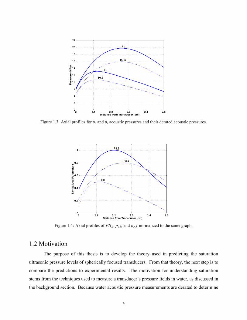
The result above provides the magnitude expected at very large values of the acoustic shock

parameter. For the regions of σ > 1 it is possible to evaluate Eq. (2.14) numerically. Figures 2.3

and 2.4 show the harmonic components calculated from Eq. (2.14) as a function of the shock

parameter. It turns out that Eq. (2.19) is a very good approximation for σ > 3. That region

between 1 and 3 is the point where a wave starts to become distorted. That transition from 1 to 3

has been evaluated and is known as Blackstock’s bridging function [8].

In summary, an acoustic shock parameter σ describes the amount of distortion associated

with a propagating wave. A Fourier analysis of the propagating plane wave yielded the

harmonic amplitudes. The evaluation was shown for both small (σ < 1) and large (σ >3) shock

parameters. The region 1 ≤ σ ≤ 3 is a transition region that can be evaluated numerically.

Figure 2.3: Fundamental frequency characteristics. The region for σ < 1 is known as the Fubini solution, and the region for σ > 3 is the sawtooth solution. Adding the two together in the transition region yields the continuous curve for B1 [8].

2.3 Saturation in Plane Waves The previous section shows the effect that a large shock parameter has on the energy

available in the signal’s fundamental. As σ approaches large values, the wave becomes

saturated. Notice in Figure 2.4 that as σ increases the amplitude of the second and third

harmonics approach that of the first (although never overtaking it). The percentage of energy in

the higher harmonics increases during saturation conditions.

12

Figure 2.4: Behavior of 1st, 2nd, and 3rd harmonics as a function of shock parameter [8].

To determine the theoretical saturation pressure for a plane wave, the wave is converted

into its Fourier components [8]:

p =2po

1 + !( )sin(n "# " t)

nn=1

$

% , σ � 1 (2.20)

which is similar to the Eq. (2.18) in the previous section. If an inverse transform of this equation

is taken, the time-domain waveform is described as

p =po (!)

1 + "( ) (2.21)

As σ becomes quite large, 1+σ ≈ σ, and the saturation can be found by

p =po(! )

"=

po!

# $uoco$k $x

=po! $%oco

2

# $ po $ k $ x=

%oco3

2# $f $ x= Psat, p , σ � 1 (2.22)

This is the result obtained for Eq. (185) in Chapter 4 of [8], and Eq. (1) in [5]. Therefore the

saturation pressure of a plane wave, Psat,p, is a function of the medium propagation speed co, the

medium density ρo, the nonlinear propagation constant β, the source frequency f, and the

distance from the source x. The subscript p indicates plane wave propagation.

13

2.4 Summary Plane wave propagation is the simplest scenario for analyzing nonlinear conditions.

Plane waves are relatively easy to analyze mathematically, which is why time was spent

developing certain ideas from them. From the analysis, it was discovered that there exists a

condition when a sinusoidal waveform no longer exhibits linear conditions, i.e., that point when

the acoustic shock parameter approaches a value of 1. This condition can be seen in Figure

2.1(c). If the wave continues to propagate until the shock parameter reaches 3 (Figure 2.1(e))

then the signal will no longer be sinusoidal but sawtooth in shape.

It was shown that for large shock parameters the amount of energy associated with the

fundamental frequency diminishes. At large values of σ, the higher harmonics obtain a larger

percentage of the overall energy. This situation led to the development of the saturation pressure

equation for plane waves.

The saturation pressure for a plane wave Psat,p has several variables associated with it.

However, the dominant variables in the equation are the source frequency f and the distance

traveled x. This states that if the source frequency is increased, then the saturation pressure level

will decrease. Similarly, if a wave is measured at a farther distance from the source, then the

theoretical saturation level will decrease.

14

CHAPTER 3

SATURATION IN SPHERICALLY CONVERGING WAVES The previous chapter developed the saturation equation for plane wave propagation.

From that analysis, it is now possible to continue with the development of the saturation equation

for a converging beam. Some of the results will be similar to the plane wave propagation, but

with a few changes or additions. Recall from the previous chapter that the saturation equation

for a plane wave is:

Psat, p =!oco

3

2"# f # x (3.1)

whereas the theoretical equation for saturation in a converging wave is [5]

Psat=

!oco

3

2"# f # F#G

ln(G) (3.2)

Equation (3.2) is almost the same as Eq. (3.1) except for two parameters. Instead of saturation

being a function of the distance travelled by the wave x, it is now a function of the transducer’s

focal length F. In addition to the focal length dependence, a new parameter G is added to

account for the focusing gain of the spherical transducer. Equation (3.2) is developed in this

chapter, and it is used to determine the theoretical pressure saturation level for each transducer

used in the experiment.

3.1 Saturation in Focused Waves The theory of acoustic saturation for a converging wave was developed in 1959 [10], and

has been analyzed recently in [5]. The work in 1959 [10] was developed for the velocity

amplitude at the focus without the presence of diffraction effects. That work described an

15

equation for the particle velocity of an ultrasonic wave in terms of the fundamental component

(cosine term in Eq. (3.3)) and the second harmonic (sine term in Eq. (3.3)), and it is given as [10]

v =Fvo

rcos(! " t + k "r) #

$" k

2 " r co( )lnF

r

%&'

()*" Fvo( )

2

sin2 ! " t + k " r( ) (3.3)

where r is the distance traveled by the wave, F is the focal length, k is the wave number, vo is the

velocity at the source, co is the speed of sound in the medium, and β is the nonlinear propagtion

constant. Similar to plane wave propagation, the converging waves travel in the medium and

eventually will begin to exhibit characteristics of nonlinearity. At some point, as is the case with

saturation, the wave is assumed to become a sawtooth wave. Figure 3.1 shows the propagating

wave becoming a sawtooth at the point designated r from the transducer. The value for rf is the

radius of the focus, assuming the focal region is circular.

Figure 3.1: Geometry used for determining saturation in a converging wave [5].

When the travelling wave becomes a sawtooth, the amplitude of the first harmonic is

assumed to be twice the amplitude of the second harmonic [5], [10]. Taking the Fourier

Transform of the right side of Eq. (3.3) and setting the first harmonic amplitude equal to twice

the second harmonic amplitude gives

2 ! (F ! vo) =

" ! k

co

! ln F r( ) ! F !vo( )2

(3.4)

To get the point r, at which the travelling wave becomes a sawtooth, Eq. (3.4) must be solved for

r:

eq(4)! 2 " (F "vo ) =# "k

co" ln F

r( ) " F "vo( )2!

2 =# "k

co" ln F

r( ) " F "vo( )! k =$

co!

16

2co

2

!" # " F " vo

= lnF

r

$%&

'()*

r = F " e+L/ F *L =2 " c

o

2

! "# "vo

(3.5)

This result for r is the same as Eq. (A4) in [5]. Using methods described in [11], the expression

for the velocity at the focus can be written as [5], [10]

vf=F !v

o

rf

1"1

#+2$

% ! co

Fvoln

F

rf

&

'()

*+,

-.

/

01

"1

(3.6)

If the limit is taken as the applied velocity approaches ∞, then the third term in the brackets is the

determining factor, and

limvo!"vf.lim

=F # v

o

rf

2$

% # co

Fvoln

F

rf

&

'()

*+,

-.

/

01

21

=%# c

o

2$ # rfln F

rf

( ) (3.7)

The distance for rf can be expressed in terms of the source wavelength λ, the focal length F, and

the transducer radius a, when the aperture angle of the transducer is small [5], [10]:

rf=! "F

2

# " a2

(3.8)

The focusing gain, G, can be expressed as [5]

G =! " a

2

# " F (3.9)

Equation (3.9) can be substituted back into Eq. (3.8), which gives

rf=F

G (3.10)

Equation (3.10) can be subsituted into Eq. (3.7), which yields the velocity limit at the focus as

vf. lim

=!" c

o

2# " rfln F

rf

( )=

! " co

2# "F

Gln F

F / G( )$%&

'()

=co

2

2# " F "f"G

ln(G) (3.11)

The velocity is converted to the saturation pressure at the focus by multiplying with the density

ρο and speed of sound co, which yields the saturation equation:

Psat= !

o"covf. lim

=!o" c

oco

2

2#"F " f"G

ln(G)=

!o" c

o

3

2#"F " f"G

ln(G)

17

This equation is the same as Eq. (3.1) in this chapter.

3.2 Theoretical Results for the Transducers Used From Eq. (3.2), the saturation for a spherically focused transducer can be predicted. In

this experiment there were seven transducers used, as shown in Table 3.1. Each transducer used

was 1.9 cm in diameter (Matec, Inc. or Panametrics, Inc.). Also shown in Table 3.1 are the four

nominal focal lengths used. The diameter and nominal focal length are used to describe the

transducer by its f/#, where # is the ratio of the nominal focal length to the diameter of the

transducer. For example, f/3 designates a transducer with a nominal focal length three times

longer than its diameter. The 9-MHz transducers included an f/3 and an f/2; the 6-MHz

transducers included an f/2 and an f/1; the 3-MHz transducers included an f/2 and an f/1; and the

7.5-MHz transducer was an f/4.5. Each of the measured values in Table 3.1 were obtained using

the wire technique [12]. A complete list of each transducer’s characteristics is given in

Appendix A.

Table 3.1: Nominal and measured transducer characteristics.

Transducer Serial #

f/# Nominal

Frequency (MHz)

Measured Frequency

(MHz)

Nominal Focal

Length (cm)

Measured Focal

Length (cm)

Measured -6dB

beamwidth (cm)

98C164 3 9 8.37 5.7 5.2 526.7� 10-4

00064 2 9 8.23 3.8 3.9 436.7� 10-4

98C151 2 6 5.64 3.8 4.0 447.6� 10-4

00068 1 6 5.58 1.9 2.1 325.8� 10-4

00059 2 3 2.83 3.8 4.3 420.3� 10-4

98C160 1 3 2.82 1.9 2.1 466.2� 10-4

V380* 4.5 7.5 6.55 8.55 7.1 859.1� 10-4

* Panametrics transducer

18

3.2.1 Determining the gain factor The value for the gain of a focusing transducer can be obtained using different methods.

The first is simply an application of the geometry of the transducer. The value for G is [5], [11]

G =zr

F=!( a

2)

"F (3.12)

where zr is the Rayleigh distance, and F is the focal length. The Rayleigh distance is described

by the radius of the transducer a and the wavelength of the source pulse λ in Eq. (3.12).

Typically this value for G is applicable only when the aperature angle (φ in Figure 3.2 below) is

small or when the focal length is long compared to the transducer’s diameter. Four different

focal lengths were used in this experiment. Table 3.2 shows the theoretical aperture angles for

all four nominal focal lengths. For the focusing gain of Eq. (3.12), it would be expected that the

f/4.5 and f/3 transducers would have the best approximation for G.

Figure 3.2: Geometry of spherically focused transducer.

Table 3.2: Theoretical aperture angles for each nominal focal length.

f/# F (cm) φ

4.5 8.55 12.7°

3 5.7 18.9°

2 3.8 28.1°

1 1.9 53.1°

There is another approach that may be applied to find an approximate value for the

focusing gain of the transducer. This technique uses the square root of the ratio of the source

area As to the focal area Af [1], [13], [14]:

G =As

Af

(3.13)

19

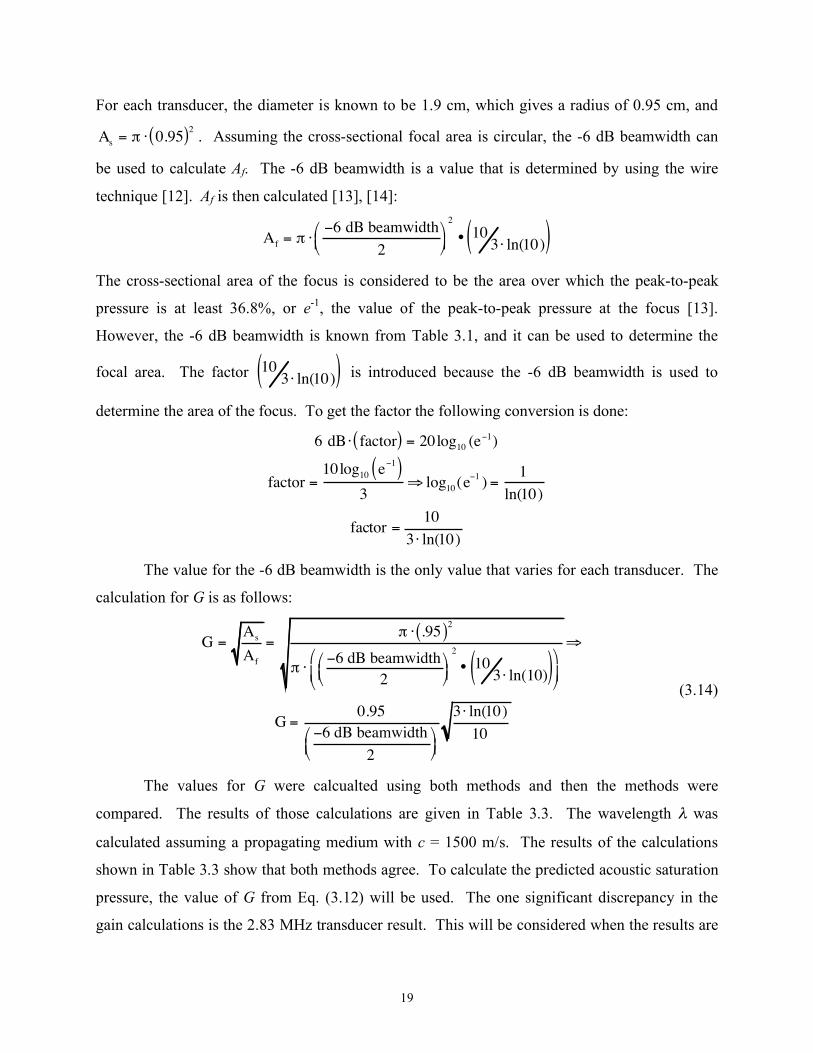
For each transducer, the diameter is known to be 1.9 cm, which gives a radius of 0.95 cm, and

As= ! " 0.95( )2 . Assuming the cross-sectional focal area is circular, the -6 dB beamwidth can

be used to calculate Af. The -6 dB beamwidth is a value that is determined by using the wire

technique [12]. Af is then calculated [13], [14]:

Af= ! "

#6 dB beamwidth

2

$%&

'()

2

• 103 " ln(10)( )

The cross-sectional area of the focus is considered to be the area over which the peak-to-peak

pressure is at least 36.8%, or e-1, the value of the peak-to-peak pressure at the focus [13].

However, the -6 dB beamwidth is known from Table 3.1, and it can be used to determine the

focal area. The factor 10 3 ! ln(10)( ) is introduced because the -6 dB beamwidth is used to

determine the area of the focus. To get the factor the following conversion is done:

6 dB ! factor( ) = 20log10 (e"1)

factor =10log10 e

"1( )3

# log10(e"1

) =1

ln(10)

factor =10

3 ! ln(10)

The value for the -6 dB beamwidth is the only value that varies for each transducer. The

calculation for G is as follows:

G =As

Af

=! " .95( )

2

! "#6 dB beamwidth

2

$%&

'()

2

• 103 " ln(10)( )$

%&

'

()

*

G =0.95

#6 dB beamwidth

2

$%&

'()

3 " ln(10)

10

(3.14)

The values for G were calcualted using both methods and then the methods were

compared. The results of those calculations are given in Table 3.3. The wavelength λ was

calculated assuming a propagating medium with c = 1500 m/s. The results of the calculations

shown in Table 3.3 show that both methods agree. To calculate the predicted acoustic saturation

pressure, the value of G from Eq. (3.12) will be used. The one significant discrepancy in the

gain calculations is the 2.83 MHz transducer result. This will be considered when the results are

20

analyzed. If for some reason the theoretical saturation does not compare with the experimental

result, then the theoretical equation may need to use the gain calculated using the area technique.

Table 3.3: Table of values used to calculate G two different ways.

Frequency1 (MHz) λ (cm) F1 (cm) G* -6 dB beamwidth1 (cm) G**

8.37 0.0179 5.2 30.5 526.7� 10-4 30.0

8.23 0.0182 3.9 39.9 436.7� 10-4 36.1

5.64 0.0266 4.0 26.6 447.6� 10-4 35.3

5.58 0.0269 2.1 50.2 325.8� 10-4 48.5

2.83 0.0530 4.3 12.4 420.3� 10-4 37.6

2.82 0.0532 1.9 28.0 466.2� 10-4 33.9

6.55 0.023 7.1 17.4 859.1� 10-4 18.4

*focusing gain calculated from Eq. (3.12) **focusing gain calculated from Eq. (3.14) 1measured parameters

3.2.2 Nonlinearity in converging waves The technique of using the cross-sectional focal area to determine the focusing gain is

reliable when σ < 1 [13]. However, this σ is the description of nonlinearity in plane waves, not

spherically converging waves. A new parameter σm was developed [13] to describe nonlinearity

at the focus of medical ultrasonic transducers, and it is defined as [13], [14]:

!m =2" # f #$ # pm #F # ln G + G2 %1( )

&# co3 G2 %1

(3.15)

where f is the source frequency, F is the focal length, β is the nonlinear propagation coefficient,

G is the focusing gain, ρ is the medium density, and co is the speed of sound. The value pm is the

average of pc and pr at the transducer focus. The average is taken because nonlinear propagation

causes the peak acoustic pressure for pc to become significantly larger than pr.

To convert back to the acoustic shock parameter developed in Chapter 2, the following

conversion is made [13]:

! =!m

sin !m( )

(3.16)

21

From the development of the acoustic shock parameter in Chapter 2, if σ >3, then the converging

acoustic pressure wave is severely distorted.

3.2.3 Determining the theoretical saturation The theoretical acoustic pressure saturation equation, as developed earlier, is

Psat=

!oco

3

2"# f # F#G

ln(G)

The density ρo, the speed of sound co, and the nonlinear propagation constant β, were held

constant at 998 kg⋅m-3, 1500 m⋅s-1, and 3.5, respectively, for each calculation of the theoretical

Psat. The measured frequencies and focal lengths from Table 3.1, and the focusing gain

calculated from Eq. (3.12) were also used. Table 3.4 provides the theoretical Psat for each

transducer used in the experiment.

Table 3.4: Frequency, focal length, and gain used to calculate the

theoretical pressure saturation level for each transducer.

f (MHz)* F (cm)* G** Psat (MPa)

8.37 5.2 30.5 9.9

8.23 3.9 39.9 16.2

5.64 4.0 26.6 17.3

5.58 2.1 50.2 52.6

2.83 4.3 12.4 19.5

2.82 2.1 28.0 68.3

6.55 7.1 17.4 6.3

*measured parameters **gain calculated from Eq. (3.12)

There are some interesting aspects of the saturation equation that can be seen from Table

3.4. For transducers of the same frequency, but different focal lengths, the transducer with the

longest focal length has the lowest saturation level. The transducer with the shortest focal length

has the highest pressure saturation level. Also, for transducers of the same focal length, the

22

transducer with the lowest frequency has the highest pressure saturation level. These are the

relations that will be analyzed in the results. Figure 3.3 shows the effect that varying the focal

length and the frequency has on the acoustic pressure saturation level.

Figure 3.3: Psat levels for 3 MHz (•), 6 MHz (−), and 9 MHz (•−) transducers at various focal lengths for G, ρo, co, and β equal to 30, 998 kg⋅m-3, 1500 m⋅s-1, and 3.5, respectively.

3.3 Summary This chapter began by developing the acoustic pressure saturation equation for

spherically focused transducers. Equation (3.2) was developed from the predicted particle

velocity of the propagating wave at the focus. Two major assumptions were made in the

derivation of Eq. (3.2). The first was that the focus was circular, and the second was that

diffraction effects were negligible.

In Section 3.2, the theoretical saturation pressures were calculated for each transducer.

To find the theoretical saturation pressures, the frequency and focal length were measured [12],

the speed, density, and nonlinear propagation constant were held constant, and the focusing gain

was determined from Eq. (3.12). A second method for finding the focusing gain was provided,

and those results were comparable to the first method. Section 3.2 ended with calculations of the

23

theoretical saturation pressures for each transducer. The Psat values shown in Table 3.4 will be

compared to the experimental results in Chapter 5.

24

CHAPTER 4

EXPERIMENTAL PROCEDURES A system was developed to find the acoustic pressures at the focus of an ultrasonic

transducer. This chapter will discuss both data acquisition and data processing.

4.1 Data Acquisition The first step in determining the acoustic pressure values at the transducer focus is

finding the transducer’s beam axis. The beam axis is defined as “a straight line joining points of

maximum pulse intensity integral measured at several different distances in the far field” [2, p.1]

To determine the beam axis, an automated procedure is used that employs a positioning system

(Daedal Inc., Harrison City, PA) with ±2 µm accuracy, an oscilloscope (LeCroy Model 9354TM,

Chestnut Ridge, NY), a high-powered, pulsed source (RAM5000, Ritec, Inc., Warwick, RI), a

PVDF hydrophone (Marconi, Ltd., Essex, England), transducers (Matec Instruments, Inc.,

Hopkinton, MA, and Panametrics, Inc., Waltham, MA), a tank with degassed water, and a

controlling computer (Dell Pentium-II) as seen in Figure 4.1. The Dell computer contains the

C++ (Microsoft Visual C++ 5.0) software used to control the positioning system and the

oscilloscope. After data collection is completed, the data are transferred to a workstation (SUN

UltraSparc) for off-line analysis. The data acquisition process requires three steps: (1) manual

setup, (2) automated determination of the maximum PII as a function of distance from the source

for calculation of the beam axis, and (3) collection of RF waveforms along the beam axis.

25

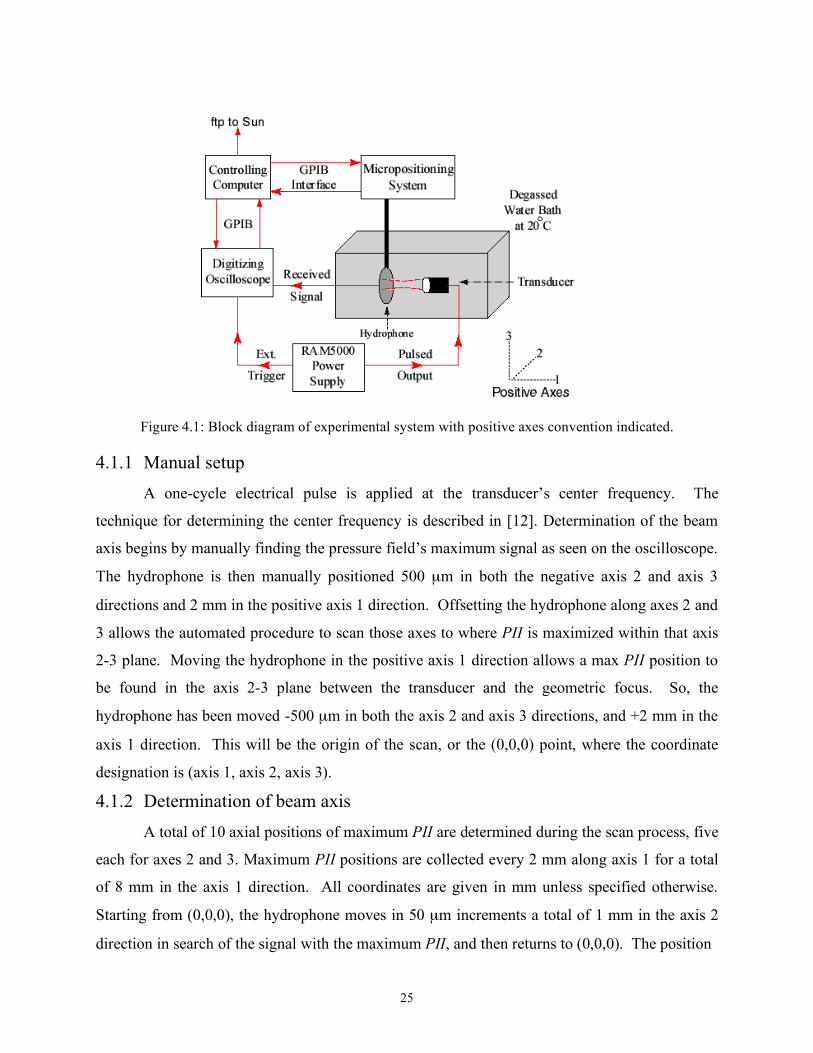
Figure 4.1: Block diagram of experimental system with positive axes convention indicated.

4.1.1 Manual setup

A one-cycle electrical pulse is applied at the transducer’s center frequency. The

technique for determining the center frequency is described in [12]. Determination of the beam

axis begins by manually finding the pressure field’s maximum signal as seen on the oscilloscope.

The hydrophone is then manually positioned 500 µm in both the negative axis 2 and axis 3

directions and 2 mm in the positive axis 1 direction. Offsetting the hydrophone along axes 2 and

3 allows the automated procedure to scan those axes to where PII is maximized within that axis

2-3 plane. Moving the hydrophone in the positive axis 1 direction allows a max PII position to

be found in the axis 2-3 plane between the transducer and the geometric focus. So, the

hydrophone has been moved -500 µm in both the axis 2 and axis 3 directions, and +2 mm in the

axis 1 direction. This will be the origin of the scan, or the (0,0,0) point, where the coordinate

designation is (axis 1, axis 2, axis 3).

4.1.2 Determination of beam axis A total of 10 axial positions of maximum PII are determined during the scan process, five

each for axes 2 and 3. Maximum PII positions are collected every 2 mm along axis 1 for a total

of 8 mm in the axis 1 direction. All coordinates are given in mm unless specified otherwise.

Starting from (0,0,0), the hydrophone moves in 50 µm increments a total of 1 mm in the axis 2

direction in search of the signal with the maximum PII, and then returns to (0,0,0). The position

26

Figure 4.2: Hydrophone movement along axes -2 and -3. The hydrophone

scans each axis for a maximum PII signal. where the PII was maximized is stored for later use. The same procedure is done for the axis 3

direction. Figure 4.2 shows hydrophone movements for axes 2 and 3. Two positions exist where

the PII is a maximum, one each for axis 2 and axis 3. The procedure in Figure 4.2 is repeated at

(2,0,0), (4,0,0), (6,0,0), and (8,0,0). The two positions found in each axis 1 plane correspond to

the axis 2 and axis 3 coordinates of the maximum PII, as shown in Figure 4.3. By definition of

the beam axis [2], those 5 coordinates of maximum PII for each position along axis 1 can be

used to create a best fit line that corresponds to the transducer’s beam axis.

Figure 4.3: Max PII positions are found along axis-2 and -3 in the axis-1 plane,

and those two positions correspond to the coordinates of the max PII in the axis-1 plane.

27

4.1.3 Waveform collection After the beam axis is calculated, the hydrophone moves back to (0, x, y), where x and y

are the beam axis positions in axis 2 and 3 when axis 1 is at zero. The hydrophone moves in 50-

µm increments along the beam axis, and collects RF waveforms at 500 Ms/s. The waveforms

are transferred to the Sun workstation where they are analyzed using Matlab®. The C++ code

used for the data acquisition is contained in Appendix B.

4.2 Data Processing In Matlab, a program calculates pressure values using voltage-to-pressure conversions

provided with the calibrated hydrophone. The hydrophone was calibrated from 1 MHz up to 20

MHz. The calibration factor varies from 0.041 to 0.043 V/MPa from 1 MHz to 15 MHz. The

calibration factor of 0.0425 V/MPa was used during this experiment, which is an average of the

factors over the stated frequency range. The code used to analyze the data is given in Appendix

C. The processing program reads in the collected data. For each waveform the program

calculates the PII, finds the maximum (pc) and minimum (pr) pressures, and then plots a smooth

version of all three. To show that the smoothing does not alter the data significantly, Figure 4.4

shows a typical RF data curve for the maximum pc values and then a best fit curve to that RF

data.

Figure 4.4: Noisy RF collected data (─) and smoothed version (·) of noisy data.

28

The best-fit curve is applied using two functions in Matlab. The first function is

“polyfit,” which generates a one-dimensional matrix that best fits the measured RF data

collected with the hydrophone (solid line in Figure 4.4). Then the “polyval” function is

performed to apply the dimensions of the distance from the transducer to the curve. As can be

seen in Figure 4.4, the “polyfit” curve fits the RF data accurately. The best-fit curve

maximum occurs around 4.8 MPa, and the RF data fluctuates from approximately 4.7 to 5 MPa

around the polyfit maximum. The whole purpose of the smoothing is to eliminate spurious noise

associated with measurement of real-time signals. The smoothing allows for the peak of the

curve to be taken as the maximum value, instead of a noise spike, which may not be associated

with the peak of the curve.

Also analyzed in Matlab is the waveform associated with the maximum value of the PII

curve. This value corresponds to the location of the focus in water. An example of the

waveform at the focus is shown in Figure 4.5. After the waveform at the focus is found, a

Fourier analysis can be performed in order to determine the fundamental and harmonic

components at the focus, as seen in Figure 4.6. This can also be done for every waveform

collected, and a plot of the fundamental and its harmonics can be plotted as a function of distance

from the transducer. The frequency analysis program is given in Appendix D.

Figure 4.5: A typical linear time-domain pressure waveform at the focus.

29

Figure 4.6: A plot of the frequency spectrum for Figure 4.5.

4.3 Summary

This data-acquisition system finds the beam axis for a spherically focused transducer.

Processing the data collected along the transducer’s beam axis allows determination of the

overall peak values for PII, pc, and pr. Those peak pressures are analyzed in a spreadsheet and

plotted as a function of applied input voltage. Those plots allow for saturation of the fields to be

seen. Also included was a description of the frequency analysis of the collected waveforms.

Those results allow saturation to be seen in terms of the amount of energy going into higher

harmonics. All the results are presented in the next chapter.

30

CHAPTER 5

EXPERIMENTAL RESULTS This chapter presents the experimental results obtained using the procedures described in

Chapter 4. For each transducer used in the experiment, the input zero-to-peak voltage was varied

from approximately 100 V up to 2 kV. The upper end of the applied voltage was intended to

drive the ultrasonic fields at the transducer’s focus into acoustic saturation. The results show

measured acoustic pressure plotted versus the applied voltage for each transducer. Also included

are results that show the effects of varying a transducer’s focal length while keeping the

frequency constant and varying the frequency while keeping the focal length constant.

Another part of the results show time-domain plots along with the corresponding

frequency-domain plots. This analysis was done for both 9-MHz transducers at a low applied

voltage and a high applied voltage. This will explain why applying higher and higher voltages to

the transducer does not necessarily increase the acoustic pressures at the focus.

5.1 Results A total of seven 19-mm-diameter transducers were used in this experiment. The

transducers included two different focal lengths for the 9-MHz, 6-MHz, and 3-MHz transducers,

and one focal length for the 7.5-MHz transducer. The applied voltage was varied from

approximately 0.1 kV up to 2 kV. For each voltage setting the procedure discussed in Chapter 4

was performed. This process yielded maximum pc and maximum pr acoustic pressures for each

applied voltage. These results were then plotted against the applied voltage. Also included in

the plots is the average of the pc and pr values. Because of diffraction effects, the pc is larger

than pr at high applied voltages. To compensate for the difference in the two values, an

arithmetic average is taken [5], [13]. For the results of this thesis, this average peak-to-peak

31

pressure is what will be compared to the theoretical acoustic pressure saturation level. The

results obtained from varying the applied input voltage to each transducer are shown in Figures

5.1-5.7.

Each plot shows the average pc and pr from the five independent trials. For each average,

the standard deviation was calculated and is represented by error bars on each. Also indicated on

the plots is the arithmetic average peak-to-peak pressure, which is the middle plot in each of the

Figures 5.1-5.7. The standard deviation of that arithmetic average was also calculated, which is

indicated by the error bars on each of the middle plots.

Acoustic saturation can be seen in Figures 5.1, 5.2, and 5.7. As the voltage reaches the

higher levels the plots of the measured acoustic pressures begin to level off. The predicted

saturation level for Figures 5.1 and 5.7 appear lower than the predicted value. The saturation

level for Figure 5.2 appears to coincide with the predicted level.

Acoustic saturation is not seen in Figures 5.3-5.6, because the applied voltage was not

increased to a high enough level. The limitation in the applied voltage was due to three factors.

The first factor was that an excess applied voltage could damage the transducer, the second was

that the high acoustic pressures could damage the hydrophone element, and the third was that

cavitation set in. The cavitation caused the received acoustic pressure signal to fluctuate. This

fluctuation was enough to cause inaccurate measurements.

The 6-MHz f/2 results shown in Figure 5.3 may be approaching saturation, but the

applied voltage was not increased enough to be certain. The 6-MHz f/1 transducer results shown

in Figure 5.4 looks linear. Both the 3-MHz f/1 and f/2 results shown in Figures 5.5 and 5.6 look

almost exponential in acoustic pressure growth. The 3-MHz f/2 results have also increased

above the predicted saturation level.

5.2 Saturation in Varying Focal Lengths or Frequencies

From Eq. (3.2), it is expected that a transducer with the same frequency but a longer focal

length will saturate at a lower level. Similarly, a transducer with the same focal length but a

higher frequency will saturate at a lower level. Figure 5.8 shows the results for varying the focal

length, and Figure 5.9 shows the results for varying the frequency. Both figures use their

corresponding peak-to-peak average pressure from Section 5.1.

32

Figure 5.1: Peak average pc (�) and pr (×) along with the peak-to-peak average pressure (�) plotted

versus applied voltage for the 9-MHz f/3 transducer. The theoretical acoustic pressure saturation level (■) is 9.9 MPa.

Figure 5.2: Peak average pc (�) and pr (×) along with the peak-to-peak average pressure (�) plotted versus applied voltage for the 9-MHz f/2 transducer. The theoretical acoustic pressure saturation level (■) is 16.2 MPa.

0

5

10

15

20

25

30

0 0.2 0.4 0.6 0.8 1 1.2 1.4 1.6

Input (kV)

Peak Average Pc

Peak Average Pr

Peak-to-Peak Average

Predicted Saturation = 16.2 MPa

9-MHz f/2

0

2

4

6

8

10

0 0.2 0.4 0.6 0.8 1 1.2

Input (kV)

Peak Pc Average

Peak Pr Average



9-MHz f/3

33




0

5

10

15

20

25

30

0 0.2 0.4 0.6 0.8 1 1.2 1.4 1.6

Input (kV)

Peak Average Pc

Peak Average Pr



6-MHz f/2

0

10

20

30

40

50

60

0 0.2 0.4 0.6 0.8 1 1.2 1.4 1.6 1.8

Input (kV)

Peak Average Pc

Peak Average Pr



6-MHz f/1

34




0

5

10

15

20

25

30

35

40

0 0.2 0.4 0.6 0.8 1 1.2 1.4 1.6 1.8 2

Input (kV)

Peak Average Pc

Peak Average Pr



3-MHz f/2

0

10

20

30

40

50

60

70

80

0 0.2 0.4 0.6 0.8 1 1.2 1.4

Input (kV)

Peak Average Pc

Peak Average Pr



3-MHz f/1

35


versus applied voltage for the 7.5-MHz f/4.5 transducer. The theoretical acoustic pressure saturation level (■) is 6.3 MPa .

Figure 5.8 shows the results obtained from the 9 MHz f/3 and f/2 transducers. The f/3

transducer saturates at a lower level than the f/2 transducer. Figure 5.9 shows results obtained

from the 9, 6, and 3 MHz, f/2 transducers. Although saturation is not seen for each transducer,

the 3-MHz transducer reaches the highest measured acoustic pressures, the 6-MHz reaches the

second highest, and the 9-MHz transducer reaches the lowest acoustic pressures. It is expected

that this trend would continue into saturation because of the theoretical relationship describing

saturation in converging waves. 5.3 Frequency Spectrum Analysis An interesting way to look at the measured acoustic pressure waveforms is through a

frequency spectrum analysis. As stated in Chapter 4, the fundamental and its harmonic

components can be analyzed. This analysis provides another way for seeing the amount of

nonlinear distortion and saturation associated with measured acoustic pressure waveforms. Two

transducers that showed acoustic saturation effects were the 9-MHz f/3 and f/2 transducers. Two

different analyses were performed on both transducer’s measured data. The first analysis looks

at the case when the transducer is driven by a low voltage, and the second when the transducer is

driven by a high voltage.

0

1

2

3

4

5

6

7

0 0.1 0.2 0.3 0.4 0.5 0.6 0.7 0.8 0.9

Input (kV)

Peak Average Pc

Peak Average Pr



7.5-MHz f/4.5

36

Figure 5.8: Peak-to-peak average pressure for 9-MHz f/3 (�) and 9-MHz f/2 (■) transducers plotted versus applied voltage. As expected, the f/3 transducer saturated at a lower level than the f/2.

Figure 5.9: Peak-to-peak average pressure for the 9-MHz (�), 6-MHz (■), and 3-MHz (�) f/2 transducers plotted versus applied voltage. The 9-MHz transducer is saturating, the 6-MHz transducer is still rising linearly with applied voltage, and the 3-MHz transducer is rising significantly higher than both the lower frequency transducers. This is the expected trend for same focal length transducers.

0

2

4

6

8

10

12

14

16

18

0 0.2 0.4 0.6 0.8 1 1.2

Input (kV)

9 MHz f/3

9 MHz f/2

0

5

10

15

20

25

0 0.2 0.4 0.6 0.8 1 1.2 1.4 1.6 1.8 2

Input (kV)

9 MHz

6 MHz

3 MHz

f/2 Transducers

37

Provided in this analysis is a plot of the acoustic pressure waveform at the transducer’s

focus in water. Performing the fast Fourier transform (FFT) on the waveform at the focus

provides the magnitudes of the fundamental, second harmonic, and third harmonic. This

presentation of data is similar to data presented in [15]. The magnitudes of the fundamental,

second harmonic, and third harmonic can also be plotted as functions of distance from the

transducer. This is similar to data presented in [16].

Figure 5.10(a) shows the waveform measured at the focus of the 9-MHz f/3 transducer

with the applied voltage low. Figure 5.10(b) corresponds to the frequency spectrum of Figure

5.10(a), and it clearly shows the fundamental and second harmonic of the waveform at the focus.

The third harmoic is minimal at the low applied voltage. Figure 5.11 shows the fundamental,

second harmonic, and third harmonic plotted versus distance from the transducer. All

magnitudes were normalized to the maximum value of the fundamental. This figure shows that

the second harmonic is low compared to the fundamental, and that the third harmonic

approximately zero.

(a) (b) Figure 5.10: Time-domain acoustic pressure waveform for 9-MHz f/3 during low applied voltage

conditions (a), and the frequency spectrum of the time-domain waveform (b).

38

Figure 5.11: Fundamental, second, and third harmonic magnitudes for the 9-MHz f/3 transducer plotted as a function of distance from the transducer for a low applied voltage. All magnitudes normalized to the maximum magnitude value of the fundamental component.

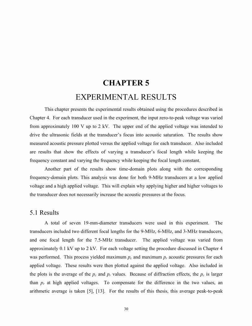
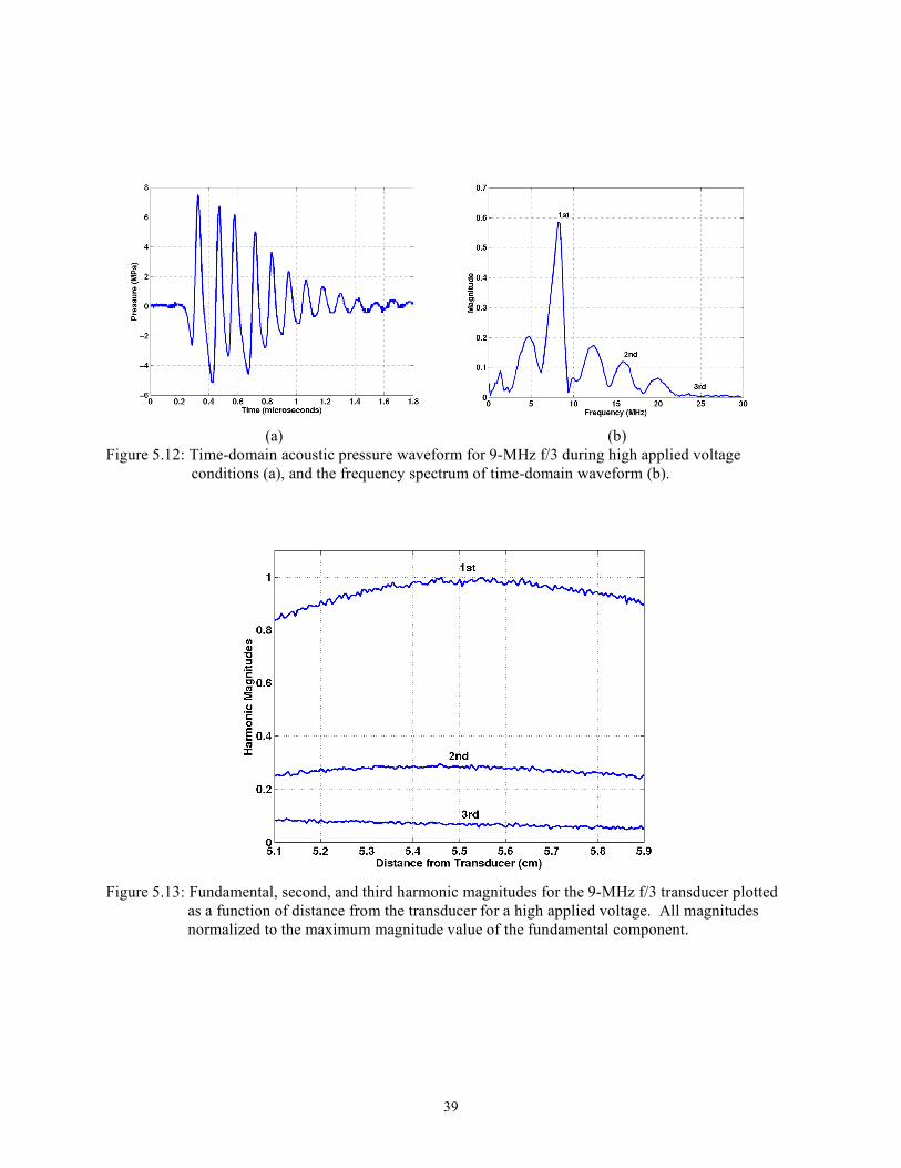
Figures 5.12 and 5.13 are similar to Figures 5.10 and 5.11, respectively. Figures 5.12 and

5.13 are measured data collected for the 9-MHz f/3 at high applied voltages. Figure 5.12(a)

shows the acoustic pressure waveform at the focus. This figure shows the highly nonlinear

conditions associated with the applied high voltage. Performing the FFT on Figure 5.12(a)

yields the result of Figure 5.12(b). The fundamental, second, and third harmonics are labeled in

Figure 5.12(b). Figure 5.13 shows the harmonic components plotted versus the distance from the

transducer. This figure shows that the second harmonic magnitude is a larger percentage of the

fundamental than that shown in Figure 5.11.

Figures 5.14 and 5.15 represent data collected from the 9-MHz f/2 transducer during low

applied voltages. Similar to previous figures, Figure 5.14(a) shows the acoustic pressure

waveform at the focus, and Figure 5.14(b) shows the frequency spectrum. The time domain

waveform in Figure 5.14(a) looks basically sinusoidal because a low applied voltage was used.

Again, the harmonic components in Figure 5.14(b) are labeled. Figure 5.15 is the plot

showing harmonic magnitudes versus the distance from the transducer.

39

(a) (b) Figure 5.12: Time-domain acoustic pressure waveform for 9-MHz f/3 during high applied voltage

conditions (a), and the frequency spectrum of time-domain waveform (b).

Figure 5.13: Fundamental, second, and third harmonic magnitudes for the 9-MHz f/3 transducer plotted as a function of distance from the transducer for a high applied voltage. All magnitudes normalized to the maximum magnitude value of the fundamental component.

40

(a) (b) Figure 5.14: Time-domain acoustic pressure waveform for 9-MHz f/2 during low applied voltage



41

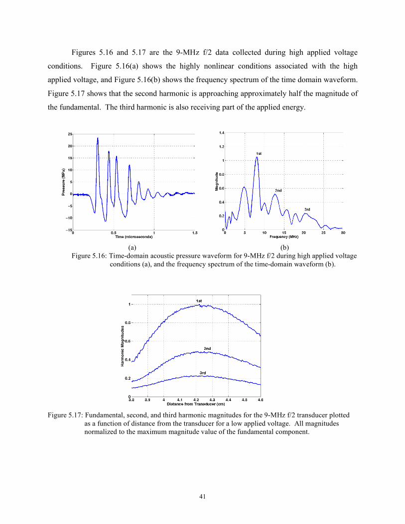
Figures 5.16 and 5.17 are the 9-MHz f/2 data collected during high applied voltage

conditions. Figure 5.16(a) shows the highly nonlinear conditions associated with the high

applied voltage, and Figure 5.16(b) shows the frequency spectrum of the time domain waveform.

Figure 5.17 shows that the second harmonic is approaching approximately half the magnitude of

the fundamental. The third harmonic is also receiving part of the applied energy.

(a) (b) Figure 5.16: Time-domain acoustic pressure waveform for 9-MHz f/2 during high applied voltage



42

5.4 Summary This chapter showed results obtained for seven diffferent transducers. The 9-MHz

transducers and the 7.5-MHz transducer showed acoustic saturation at the focus. The lower-

frequency transducers still showed signs of increasing acoustic pressure at the focus at the high

end of the applied voltage. The voltage was limited because the transducers could be damaged

from the high voltage, the hydrophone could be damaged from the high acoustic pressures, or

cavitation caused the waveforms to become unstable.

Figure 5.8 showed how varying the focal length while keeping the frequency constant

effects the saturation level. The shorter focal length transducer saturated at a higher level than

the longer focal length. Figure 5.9 showed how varying the frequency while keeping the focal

length constant effects saturation level. The lower frequency transducers were reaching higher

acoustic pressures. Figures 5.10-5.17 showed the frequency spectrum for both a low applied

voltage and a high applied voltage for the 9-MHz f/2 and f/3 transducers. From that information,

it was shown that the high applied voltages created a more nonlinear time domain pressure

waveform at the focus. The frequency spectrum of that time domain waveform showed

significant magnitude contributions from the second harmonics.

43

CHAPTER 6

DISCUSSION AND CONCLUSIONS This chapter discusses the results from Chapter 5 and compares those results to existing

studies. This chapter also presents conclusions made from the results.

6.1 Discussion Literature exists that analyzes the effects of acoustic saturation in spherically focused

waves. In [14], a 3.5-MHz f/4 transducer was analyzed that had a focusing gain of 6.3. The

experimental results for that transducer show acoustic saturation at approximately 2 MPa. If the

theoretical calculations were done using the parameters stated in [14], then the Psat would be

approximately 5.9 MPa. This is higher than what was measured in the experiment of [14].

Another transducer analyzed was a 2.5-MHz f/4.6 transducer with a focusing gain of 2.5.

However, the nonlinear propagtion was easier to attain in the higher frequency transducer, so the

results focused on the first transducer. The study [14] agreed with the results of this thesis in two

ways. First, the experimental results in [14] saturated at a lower level than the theoretical

saturation level, which agrees with the results obtained for the 9-MHz f/3 transducer. This

underestimation in the experiment may be due to the longer focal length transducers. Secondly,

the fact that the lower frequency transducer was more difficult to drive into nonlinear conditions

agrees with the results obtained in this thesis. Although the focusing gains are much higher in

this thesis, the lower frequency transducers did not saturate because they were more difficult to

drive into nonlinear conditions.

In another study [17], a 0.8-inch diameter, 450-kHz transducer was analyzed. The waves

were not focused, but the ultrasonic pressure waves were measured at various distances from the

44

transducer. When the hydrophone was a relatively long distance away, the transducer saturated

at a lower applied voltage, and the saturation pressure was lower. This agrees with experimental

results presented for the two focal length results of Figure 5.8. Also shown in [17] is the

difficulty associated with driving a transducer’s ultrasonic fields to saturation when the

hydrophone is close to the transducer. In [17], when the hydrophone was the closest to the

transducer, the measured acoustic pressures continued to rise linearly with applied power. This

result is similar to the 6-MHz f/2 and f/1 results shown in Figures 5.3 and 5.4. This also agrees

with the Psat equation because of the inverse focal length dependence on pressure saturation

level.

Two studies [15], [16] looked at the magnitude levels of the fundamental, second, and

third harmonics. In [16], the magnitude levels were plotted as functions of distance from the

transducer. It was shown that during nonlinear conditions the second and third harmonics

become more significant. In [15] measurements were made through tissue (porcine kidney).

Similar to [16], plots of the fundamental, second, and third harmonic magnitudes were plotted

versus distance from the transducer. The tissue made the acoustic pressure waveforms more

nonlinear, which increased the magnitudes of the second and third harmonics.

In this thesis, a frequency analysis was done on the 9-MHz f/3 and f/2 transducers. The

results of those plots show the effects of nonlinear propagation, which is similar to other results

[15], [16]. The hydrophone did not have a high enough bandwidth to make an accurate

measurement of the third harmonic components. The plots of the fundamental, second, and third

harmonics in this thesis are intended to show the extent of nonlinear propagation, not necessarily

the true magnitudes of the harmonics.

6.2 Conclusions The experimental results show that some transducers saturated, whereas others did not.

The higher frequency, longer focal length transducers demonstrated the most obvious acoustic

saturation effects. The 9-MHz f/2 transducer had a peak-to-peak average pressure that was

approximately the same as the predicted saturation level. The peak-to-peak average acoustic

pressures for the 9-MHz f/3 and 7.5-MHz f/4.5 transducers were lower than the predicted levels.

The other transducers were not driven into acoustic saturation. This was due to

equipment and transducer limitations. However, each transducer showed signs of nonlinearity at

45

the higher end of the applied voltage. Acoustic saturation is known to occur during nonlinear

propagation. This implies that if the transducers could be driven harder, then they would

eventually saturate. The theory states that it would be more difficult to saturate a shorter focal

length, lower frequency transducer, because the pressure levels will be extremely high, as seen in

Figure 3.3. This was verified in the experiment.

The results agree with the theory in many aspects. From the definition of Psat

Pc

f F

G

Gsat

o o=! !

!"

#

3

2 ln( )

it would be expected that longer focal length transducers of the same frequency will saturate at a

lower level, which was shown in Figure 5.8. The 9-MHz f/3 saturates at a lower acoustic

pressure than the 9-MHz f/2, which agrees with the Psat equation. Similarly, the 6-MHz f/2

transducer was reaching lower acoustic pressures than the 6-MHz f/1 for the same applied

voltages, as was the 3-MHz f/2 reaching lower acoustic pressures than the 3-MHz f/1 for the

same applied voltage.

It would also be expected that transducers of the same focal length but lower frequencies

will saturate at higher acoustic pressure levels. This was verified in the results of Figure 5.9.

The 9-MHz f/2 saturated while the 6-MHz f/2 was still increasing. The 3-MHz f/2 was rising

higher than both. There was one interesting result from this analysis. The 9-MHz transducer

was reaching higher pressure levels at lower applied voltages than both the 6- and 3-MHz

transducers. This may be attributed to nonlinear propagation. For example, the 9-MHz

transducer saturates at a lower applied voltage, which means that the acoustic pressure fileds

begin to exhibit characteristics of nonlinearity at lower applied voltages. Nonlinearity indicates

that pc is greater than pr for spherically focused acoustic waves. The fact that pc is greater means

that the average peak-to-peak pressure will be greater for the 9-MHz transducer at lower applied

voltages.

A frequency analysis was performed on both the 9-MHz f/3 and f/2 transducer fields at

the focus. During applied high voltage conditions, the time-domain waveform collected at the

transducer’s focus looked highly nonlinear. When a frequency analysis was performed on the

time-domain waveform, the magnitudes of the second and third harmonics helped show the

severity of nonlinearity. For example, in Figure 5.17 the fundamental, second, and third

harmonics are plotted versus distance from the 9-MHz f/2 transducer. The peak of the second

46

harmonic is approximately 50% the peak of the fundamental, and the peak of the third harmonic

is approximately 20%. Conversely, during linear conditions in Figure 5.15, the peak of the

second harmonic is approximately 30% the peak of the fundamental, and the peak of the third

harmonic is approximately 10% of the fundamental.

There is an interesting effect shown in Figures 5.12 and 5.16, which are the applied high

voltage waveforms collected at the focus. In Figure 5.12(b) there is a half harmonic and a 1.5

harmonic shown in the frequency spectrum and both have a higher peak magnitude than the

second harmonic. Figure 5.16(b) is similar in that the half harmonic component is larger than the

second harmonic. This must be an additional effect of nonlinear propagation.

The experimental results in this thesis agree with theoretical predictions. They also

compare with other studies that have been conducted on acoustic saturation in spherically

converging waves. The advantage of this study was that the number of transducers was not

limited. Seven transducers with various frequencies and focal lengths allowed for a complete

comparison of experimental results and theoretcial predictions.

.

47

CHAPTER 7

SUMMARY AND FUTURE WORK 7.1 Summary This thesis provided the background to understand acoustic saturation in spherically

focused transducers. It began with a development of nonlinear propagation in plane waves.

From the plane wave development, it was shown that as the propagating waves approach

saturation higher harmonics receive a higher percentage of the overall energy.

The next development was for the theoretical acoustic pressure saturation equation for

spherically focused transducers. That equation was developed from the propagation speed of the

travelling acoustic waves [10] into the more familiar Psat equation [5]. For the Psat equation

several parameters were needed. The medium density ρo, the propagation speed co, and the

nonlinear propagation constant β were all held constant for calculations of Psat. The focal length

F and the frequency f were dependent upon the transducer used and were given in Table 3.1.

Two different methods for determining the gain factor G were given. The first method used the

geometry of the transducer and its operating frequency, and the second method used the -6 dB

beamwidth of the transducer. Table 3.3 shows that the two methods were comparable, so the

first method was used to calculate Psat. Table 3.4 shows the theoretical results for Psat.

Chapter 4 discussed the methodology used in measuring the acoustic pressure levels. The

system finds the beam axis, which includes the transducer’s focus, and then measures pressure

values along that beam axis. There are maximum acoustic pressure measurements for pc and pr

for each waveform collected along the beam axis. Those results were plotted as functions of

distance from the transducer to provide axial profiles. The peak value of the axial profiles was

then plotted as a function of the zero-to-peak applied voltage. Those plots were given in Chapter

5 for each of the transducers used in the experiment. Also given in the results were frequency

48

analysis plots of the 9-MHz transducers. The frequency spectra gave a comparison of linear

propagation and nonlinear propagation. The comparison was made by looking at the magnitudes

of the second and third harmonics.

7.2 Future Work The experimental system developed in this thesis is useful in determining the acoustic

pressure levels in focused ultrasonic transducers. There are many possible experiments that

could be done. It would be interesting to analyze three transducers with the same frequency and

focal length and see if the saturation is the same for each. This would allow for more

information to be collected for spherically focused transducers. A second possible experiment

would be to change the medium of propagation. It would be expected from the theory that a

more dense medium, for example, would provide a higher thoeretical Psat. A third experiment

would be to look at multielement transducers, not just spherically focused. It would be

interesting to see what aspect of the multielement transducer dominates.

78

REFERENCES [1] F. A. Duck, “Estimating in situ exposure in the presence of acoustic nonlinearity,”

Journal of Ultrasound in Medicine, vol. 18, pp. 43-53, January 1999.

[2] American Institute of Ultrasound in Medicine, Acoustic Output Measurement and

Labeling Standard for Diagnostic Ultrasound Equipment. Laurel, MD: AIUM

Publications, 1992.

[3] American Institute of Ultrasound In Medicine, Standard for Real-Time Display of

Thermal and Mechanical Acoustic Output Indices on Diagnostic Ultrasound Equipment.

Laurel, MD: AIUM Publications,1997.

[4] FDA (Food and Drug Administration), Information for Manufacturers Seeking Marketing

Clearance of Diagnostic Ultrasound Systems and Transducers. Rockville, MD: Center

for Devices and Radiological Health, US Dept. Health and Human Services, 1997.

[5] F. A. Duck, “Acoustic saturation and output regulation,” Ultrasound in Medicine and

Biology, vol. 25, pp. 1009-1018, January 1999.

[6] T. Christopher and E. L. Carstensen, “Finite amplitude distortion and its relationship to

linear derating formulae for diagnostic ultrasound systems,” Ultrasound in Medicine and

Biology, vol. 22, pp. 1103-1116, August 1996.

[7] E. L. Carstensen, D. Dalecki, S. M. Gracewski, and T. Christopher, “Nonlinear

propagation and the output indices,” Journal of Ultrasound in Medicine, vol. 18, pp. 69-

80, January 1999.

[8] D. T. Blackstock and M. F. Hamilton, Eds., Nonlinear Acoustics. San Diego: Academic

Press, 1998.

78

[9] D. G. Zill and M. R. Cullen, Advanced Engineering Mathematics. Boston: Prindle,

Weber & Schmidt-KENT Publishing, 1992.

[10] K. A. Naugol’nykh and E. V. Romanenko, “Amplification factor of a focusing system as

a function of sound intensity,” Soviet Physics-Acoustics, vol. 5, pp. 191-195, May 1959.

[11] K. A. Naugol’nykh and E. V. Romanenko, “On the propagation of finite-amplitude

waves in a liquid,” Soviet Physics-Acoustics, vol. 4, pp. 202-204, April 1958.

[12] K. Raum and W. D. O’Brien, Jr., “Pulse-echo field distribution measurement technique

for high-frequency ultrasound sources,” IEEE Transactions on Ultrasonics,

Ferroelectrics, and Frequency Control, vol. 44, pp. 810-815, July 1997.

[13] D. R. Bacon, “Finite amplitude distortion of the pulsed fields used in diagnostic

ultrasound,” Ultrasound in Medicine and Biology, vol. 10, pp. 189-195, March/April

1984.

[14] F. A. Duck and M. A. Perkins, “Amplitude-dependent losses in ultrasound exposure

measurement,” IEEE Transactions on Ultrasonics, Ferroelectrics, and Frequency

Control, vol. 35, pp. 232-241, February 1988.

[15] L. Filipczyński, T. Kujawska, R. Tymkiewicz, and J. Wójcik, “Nonlinear and linear

propagation of diagnostic ultrasound pulses,” Ultrasound in Medicine and Biology, vol.

25, pp. 285-299, March/April 1999.

[16] A. C. Baker, “A numerical study of the effect of drive level on the intensity loss from an

ultrasonic beam,” Ultrasound in Medicine and Biology, vol. 23, pp. 1083-1088, July

1997.

[17] J. A. Shooter, T. G. Muir, and D. T. Blackstock, “Acoustic saturation of spherical waves

in water,” Journal of the Acoustical Society of America, vol. 55, pp. 54-62, January 1974.

Transducer Thesis

Documents

Transcript of Transducer Thesis