User’s Manual Version 2006 - CSC · i Introduction to MOLPRO MOLPRO is a complete system of ab...
383
M OLPRO User’s Manual Version 2006.1 H.-J. Werner Institut f¨ ur Theoretische Chemie Universit¨ at Stuttgart Pfaffenwaldring 55 D-70569 Stuttgart Federal Republic of Germany P. J. Knowles School of Chemistry Cardiff University Main Building, Park Place, Cardiff CF10 3AT United Kingdom May 2006 (Copyright c 2006 University College Cardiff Consultants Limited)
Transcript of User’s Manual Version 2006 - CSC · i Introduction to MOLPRO MOLPRO is a complete system of ab...

MOLPRO
User’s ManualVersion 2006.1
H.-J. Werner
Institut fur Theoretische ChemieUniversitat StuttgartPfaffenwaldring 55D-70569 Stuttgart
Federal Republic of Germany
P. J. Knowles
School of ChemistryCardiff University
Main Building, Park Place, Cardiff CF10 3ATUnited Kingdom
May 2006
(Copyright c©2006 University College Cardiff Consultants Limited)

i
Introduction to MOLPRO
MOLPRO is a complete system of ab initio programs for molecular electronic structure calcula-tions, designed and maintained by H.-J. Werner and P. J. Knowles, and containing contributionsfrom a number of other authors. As distinct from other commonly used quantum chemistrypackages, the emphasis is on highly accurate computations, with extensive treatment of theelectron correlation problem through the multiconfiguration-reference CI, coupled cluster andassociated methods. Using recently developed integral-direct local electron correlation methods,which significantly reduce the increase of the computational cost with molecular size, accurateab initio calculations can be performed for much larger molecules than with most other pro-grams.
The heart of the program consists of the multiconfiguration SCF, multireference CI, and coupled-cluster routines, and these are accompanied by a full set of supporting features. The packagecomprises
• Integral generation for generally contracted symmetry adapted gaussian basis functions(spd f ghi). There are two programs with identical functionality: the preferred code isSEWARD (R. Lindh) which is the best on most machines; ARGOS (R. M. Pitzer) is avail-able as an alternative, and in some cases is optimum for small memory scalar machines.Also two different gradient integral codes, namely CADPAC (R. Amos) and ALASKA (R.Lindh) are available. Only the latter allows the use of generally contracted symmetryadapted gaussian basis functions.
• Effective Core Potentials (contributions from H. Stoll).
• Many one-electron properties.
• Some two-electron properties, e.g. L2x , L2
y , L2z , LxLy etc..
• Closed-shell and open-shell (spin restricted and unrestricted) self consistent field.
• Density-functional theory in the Kohn-Sham framework with various gradient correctedexchange and correlation potentials.
• Multiconfiguration self consistent field. This is the quadratically convergent MCSCFprocedure described in J. Chem. Phys. 82 (1985) 5053. The program can optimize aweighted energy average of several states, and is capable of treating both completely gen-eral configuration expansions and also long CASSCF expansions as described in Chem.Phys. Letters 115 (1985) 259.
• Multireference CI. As well as the usual single reference function approaches (MP2, SDCI,CEPA), this module implements the internally contracted multireference CI method asdescribed in J. Chem. Phys. 89 (1988) 5803 and Chem. Phys. Lett. 145 (1988) 514. Nonvariational variants (e.g. MR-ACPF), as described in Theor. Chim. Acta 78 (1990) 175,are also available. Electronically excited states can be computed as described in Theor.Chim. Acta, 84 95 (1992).
• Multireference second-order and third-order perturbation theory (MR-PT2, MR-PT3) asdescribed in Mol. Phys. 89, 645 (1996) and J. Chem. Phys. 112, 5546 (2000).
• Møller-Plesset perturbation theory (MPPT), Coupled-Cluster (CCSD), Quadratic config-uration interaction (QCISD), and Brueckner Coupled-Cluster (BCCD) for closed shellsystems, as described in Chem. Phys. Lett. 190 (1992) 1. Perturbative corrections fortriple excitations can also be calculated (Chem. Phys. Letters 227 (1994) 321).

ii
• Open-shell coupled cluster theories as described in J. Chem. Phys. 99 (1993) 5219,Chem. Phys. Letters 227 (1994) 321.
• Full Configuration Interaction. This is the determinant based benchmarking program de-scribed in Comp. Phys. Commun. 54 (1989) 75.
• Analytical energy gradients for SCF, DFT, state-averaged MCSCF/CASSCF, MRPT2/CASPT2,MP2 and QCISD(T) methods.
• Analytical non-adiabatic coupling matrix elements for MCSCF.
• Valence-Bond analysis of CASSCF wavefunction, and energy-optimized valence bondwavefunctions as described in Int. J. Quant. Chem. 65, 439 (1997).
• One-electron transition properties for MCSCF, MRCI, and EOM-CCSD wavefunctions,CASSCF and MRCI transition properties also between wavefunctions with different or-bitals.
• Spin-orbit coupling, as described in Mol. Phys., 98, 1823 (2000).
• Some two-electron transition properties for MCSCF wavefunctions (e.g., L2x etc.).
• Population analysis.
• Orbital localization.
• Distributed Multipole Analysis (A. J. Stone).
• Automatic geometry optimization as described in J. Comp. Chem. 18, (1997), 1473.
• Automatic calculation of vibrational frequencies, intensities, and thermodynamic proper-ties.
• Reaction path following, as described in Theor. Chem. Acc. 100, (1998), 21.
• Various utilities allowing other more general optimizations, looping and branching (e.g.,for automatic generation of complete potential energy surfaces), general housekeepingoperations.
• Geometry output in XYZ, MOLDEN and Gaussian formats; molecular orbital andfrequency output in MOLDEN format.
• Integral-direct implementation of all Hartree-Fock, DFT and pair-correlated methods (MP,CCSD, MRCI etc.), as described in Mol. Phys., 96, (1999), 719. At present, perturbativetriple excitation methods are not implemented.
• Local second-order Møller-Plesset perturbation theory (LMP2) and local coupled clustermethods, as described in in J. Chem. Phys. 104, 6286 (1996), Chem. Phys. Lett. 290,143 (1998), J. Chem. Phys. 111, 5691 (1999), J. Chem. Phys. 113, 9443 (2000), J. Chem.Phys. 113, 9986 (2000), Chem. Phys. Letters 318, 370 (2000), J. Chem. Phys. 114, 661(2001), Phys. Chem. Chem. Phys. 4, 3941 (2002).
• Local density fitting methods, as described in J. Chem. Phys. 118, 8149 (2003), Phys.Chem. Chem. Phys. 5, 3349 (2003), Mol. Phys. 102, 2311 (2004).
• Analytical energy gradients for LMP2 and DF-LMP2, as described in J. Chem. Phys.108, 5185, (1998), J. Chem. Phys. 121, 737 (2004).

iii
• Explicit correlation methods, as described in J. Chem. Phys. 119, 4607 (2003), J. Chem.Phys. 121, 4479 (2004), J. Chem. Phys. 124, 054114 (2006), J. Chem. Phys. 124, 094103(2006).
• Parallel execution on distributed memory machines, as described in J. Comp. Chem.19, (1998), 1215. At present, SCF, DFT, MRCI, MP2, LMP2, CCSD(T) energies andSCF, DFT gradients are parallelized when running with conventional integral evaluation;integral-direct and density fitted SCF, DFT, LMP2, and LCCSD(T) are also parallel.
The program is written mostly in standard Fortran–90. Those parts which are machine depen-dent are maintained through the use of a supplied preprocessor, which allows easy interconver-sion between versions for different machines. Each release of the program is ported and testedon a number of IBM RS/6000, Hewlett-Packard, Silicon Graphics, Compaq, and Linux systems.A fuller description of the hardware and operating systems of these machines can be found athttp://www.molpro.net/supported. The program additionally runs on Cray, Sun,Convex, Fujitsu and NEC SX4 platforms, as well as older architectures and/or operating systemsfrom the primary list; however, testing is not carried out regularly on these systems, and hand-tuning of code may be necessary on porting. A large library of commonly used orbital basis setsis available, which can be extended as required. There is a comprehensive users’ manual, whichincludes installation instructions. The manual is available in PostScript, PDF and also in HTMLfor mounting on a Worldwide Web server.
New methods and enhancements in Version 2006.1 include:
1. More consistent input language and input pre-checking.
2. More flexible basis input, allowing to handle multiple basis sets.
3. New more efficient density functional implementation, additional density functionals.
4. Low-order scaling local coupled cluster methods with perturbative treatment of triplesexcitations (LCCSD(T) and variants like LQCISD(T))
5. Efficient density fitting (DF) programs for Hartree-Fock (DF-HF), Density functionalKohn-Sham theory (DF-KS), Second-order Møller-Plesset perturbation theory (DF-MP2),as well as for all local methods (DF-LMP2, DF-LMP4, DF-LQCISD(T), DF-LCCSD(T))
6. Analytical QCISD(T) gradients
7. Analytical MRPT2 (CASPT2) and multi-state CASPT2 gradients, using state averagedMCSCF reference functions
8. Analytical DF-HF, DF-KS, DF-LMP2, and DF-SCS-LMP2 gradients
9. Explicitly correlated methods with density fitting: DF-MP2-R12/2A’, DF-MP2-F12/2A’as well as the local variants DF-LMP2-R12/2*A(loc) and DF-LMP2-F12/2*A(loc).
10. Multi-state MRPT2, MS-CASPT2
11. Coupling of multi-reference perturbation theory and configuration interaction (CIPT2)
12. DFT-SAPT
13. Transition moments and transition Hamiltonian between CASSCF and MRCI wavefunc-tions with different orbitals.
14. Douglas-Kroll-Hess Hamiltonian up to arbitrary order.

iv
15. A new spin-orbit integral program for generally contracted basis sets.
16. Improved procedures for geometry optimization and numerical Hessian calculations, in-cluding constrained optimization.
17. Improved facilities to treat large lattices of point charges for QM/MM calculations, in-cluding lattice gradients.
18. An interface to the MRCC program of M. Kallay, allowing coupled-cluster calculationswith arbitrary excitation level.
19. Automatic embarrassingly parallel computation of numerical gradients and Hessians(mppx Version).
20. Additional parallel codes, e.g. DF-HF, DF-KS, DF-LCCSD(T) (partly, including triples).
Future enhancements presently under development include
• Automatic calculation of anharmonic vibrational spectra using vibrational CI.
• Coupling of DFT and coupled cluster methods.
• Open-shell local coupled cluster methods.
• Explicitly correlated local coupled cluster methods.
• Local response methods (CC2, EOM-CCSD) for computing excitation energies and tran-sition properties in large molecules.
• Analytical energy gradients for CCSD(T)
• Analytic second derivatives for DFT
These features will be included in the base version at later stages. The above list is for infor-mation only, and no representation is made that any of the above will be available within anyparticular time.
MOLPRO on the WWW
The latest information on MOLPRO, including program updates, can be found on the worldwideweb at location http://www.molpro.net/.

v
References
All publications resulting from use of this program must acknowledge the following.
MOLPRO, version 2006.1, a package of ab initio programs, H.-J. Werner, P. J. Knowles, R.Lindh, F. R. Manby, M. Schutz, P. Celani, T. Korona, G. Rauhut, R. D. Amos, A. Bernhardsson,A. Berning, D. L. Cooper, M. J. O. Deegan, A. J. Dobbyn, F. Eckert, C. Hampel and G. Hetzer,A. W. Lloyd, S. J. McNicholas, W. Meyer and M. E. Mura, A. Nicklass, P. Palmieri, R. Pitzer, U.Schumann, H. Stoll, A. J. Stone, R. Tarroni and T. Thorsteinsson , see http://www.molpro.net .
Some journals insist on a shorter list of authors; in such a case, the following should be usedinstead.
MOLPRO, version 2006.1, a package of ab initio programs, H.-J. Werner, P. J. Knowles, R.Lindh, F. R. Manby, M. Schutz, and others , see http://www.molpro.net .
Depending on which programs are used, the following references should be cited.
Integral evaluation (SEWARD)R. Lindh, U. Ryu, and B. Liu, J. Chem. Phys. 95, 5889 (1991).
Integral-direct ImplementationM. Schutz, R. Lindh, and H.-J. Werner, Mol. Phys. 96, 719 (1999).
MCSCF/CASSCF:H.-J. Werner and P. J. Knowles, J. Chem. Phys. 82, 5053 (1985);P. J. Knowles and H.-J. Werner, Chem. Phys. Lett. 115, 259 (1985).
See also:
H.-J. Werner and W. Meyer, J. Chem. Phys. 73, 2342 (1980);H.-J. Werner and W. Meyer, J. Chem. Phys. 74, 5794 (1981);H.-J. Werner, Adv. Chem. Phys. LXIX, 1 (1987).
Internally contracted MRCI:H.-J. Werner and P.J. Knowles, J. Chem. Phys. 89, 5803 (1988);P.J. Knowles and H.-J. Werner, Chem. Phys. Lett. 145, 514 (1988).
See also:
H.-J. Werner and E.A. Reinsch, J. Chem. Phys. 76, 3144 (1982);H.-J. Werner, Adv. Chem. Phys. LXIX, 1 (1987).
Excited states with internally contracted MRCI:P. J. Knowles and H.-J. Werner, Theor. Chim. Acta 84, 95 (1992).
Internally contracted MR-ACPF, QDVPT, etc:H.-J. Werner and P. J. Knowles, Theor. Chim Acta 78, 175 (1990).
The original reference to uncontracted MR-ACPF, QDVPT, MR-ACQQ are:R. J. Gdanitz and R. Ahlrichs, Chem. Phys. Lett. 143, 413 (1988);R. J. Cave and E. R. Davidson, J. Chem. Phys. 89, 6798 (1988);P. G. Szalay and R. J. Bartlett, Chem. Phys. Lett. 214, 481 (1993).
Multireference perturbation theory (CASPT2/CASPT3):H.-J. Werner, Mol. Phys. 89, 645 (1996);P. Celani and H.-J. Werner, J. Chem. Phys. 112, 5546 (2000).
Coupling of multi-reference configuration interaction and multi-reference perturbationtheory, P. Celani, H. Stoll, and H.-J. Werner, Mol. Phys. 102, 2369 (2004).

vi
Analytical energy gradients and geometry optimizationGradient integral evaluation (ALASKA): R. Lindh, Theor. Chim. Acta 85, 423 (1993);MCSCF gradients: T. Busch, A. Degli Esposti, and H.-J. Werner, J. Chem. Phys. 94, 6708(1991);MP2 and LMP2 gradients: A. El Azhary, G. Rauhut, P. Pulay, and H.-J. Werner, J. Chem. Phys.108, 5185 (1998);DF-LMP2 gradients: M. Schutz, H.-J. Werner, R. Lindh and F. R. Manby, J. Chem. Phys. 121,737 (2004).QCISD and LQCISD gradients: G. Rauhut and H.-J. Werner, Phys. Chem. Chem. Phys. 3,4853 (2001);CASPT2 gradients: P. Celani and H.-J. Werner, J. Chem. Phys. 119, 5044 (2003).Geometry optimization: F. Eckert, P. Pulay and H.-J. Werner, J. Comp. Chemistry 18, 1473(1997);Reaction path following: F. Eckert and H.-J. Werner, Theor. Chem. Acc. 100, 21, 1998.
Harmonic frequenciesG. Rauhut, A. El Azhary, F. Eckert, U. Schumann, and H.-J. Werner, Spectrochimica Acta 55,651 (1999).
Møller-Plesset Perturbation theory (MP2, MP3, MP4):Closed-shell Møller-Plesset Perturbation theory up to fourth order [MP4(SDTQ)] is part of thecoupled cluster code, see CCSD.
Open-shell Møller-Plesset Perturbation theory (RMP2):R. D. Amos, J. S. Andrews, N. C. Handy, and P. J. Knowles, Chem. Phys. Lett. 185, 256 (1991).
Coupled-Cluster treatments (QCI, CCSD, BCCD):C. Hampel, K. Peterson, and H.-J. Werner, Chem. Phys. Lett. 190, 1 (1992) and referencestherein. The program to compute the perturbative triples corrections has been developed byM. J. O. Deegan and P. J. Knowles, Chem. Phys. Lett. 227, 321 (1994).
Equation-of-Motion Coupled Cluster Singles and Doubles (EOM-CCSD):T. Korona and H.-J. Werner, J. Chem. Phys. 118, 3006 (2003).
Open-shell coupled-cluster (RCCSD, UCCSD):P. J. Knowles, C. Hampel and H.-J. Werner, J. Chem. Phys. 99, 5219 (1993); Erratum: J. Chem.Phys. 112, 3106 (2000).
Local MP2 (LMP2):G. Hetzer, P. Pulay, and H.-J. Werner, Chem. Phys. Lett. 290, 143 (1998)M. Schutz, G. Hetzer, and H.-J. Werner, J. Chem. Phys. 111, 5691 (1999)G. Hetzer, M. Schutz, H. Stoll, and H.-J. Werner, J. Chem. Phys. 113, 9443 (2000)See also references on energy gradients and density fitting.
Local Coupled Cluster methods (LCCSD, LQCISD, LMP4):C. Hampel and H.-J. Werner, J. Chem. Phys. 104 6286 (1996)M. Schutz and H.-J. Werner, J. Chem. Phys. 114, 661 (2001)M. Schutz, Phys.Chem.Chem.Phys. 4, 3941 (2002)See also references on energy gradients and density fitting.
Local triple excitations:M. Schutz and H.-J. Werner, Chem. Phys. Lett. 318, 370 (2000);M. Schutz, J. Chem. Phys. 113, 9986 (2000).M. Schutz, J. Chem. Phys. 116, 8772 (2002).
Density fitting methods:

vii
DFT, Poisson fitting: F. R. Manby, P. J. Knowles, and A. W. Lloyd,J. Chem. Phys. 115, 9144 (2001).
DF-MP2, DF-LMP2: H.-J. Werner, F. R. Manby, and P. J. Knowles,J. Chem. Phys. 118, 8149 (2003).
DF-LCCSD: M. Schutz and F. R. Manby,Phys. Chem. Chem. Phys. 5, 3349 (2003)
DF-HF: R. Polly, H.-J. Werner, F. R. Manby, and Peter J. Knowles,Mol. Phys. 102, 2311 (2004).
DF-LMP2 gradients: M. Schutz, H.-J. Werner, R. Lindh and F. R. Manby,J. Chem. Phys. 121, 737 (2004).
DF-LCCSD(T): H.-J. Werner and M. Schutz,in prepation.
Explicitly correlated methods with density fitting:
DF-MP2-R12: F. R. Manby, J. Chem. Phys. 119, 4807 (2003).
DF-MP2-F12: A. J. May and F. R. Manby, J. Chem. Phys. 132, 4479 (2004).
DF-LMP2-R12(loc): H.-J. and F. R. Manby, J. Chem. Phys., 124, 054114 (2006).
DF-LMP2-F12(loc): F. R. Manby H.-J. Werner, T. B. Adler, and A. J. May, J. Chem. Phys.124, 094103 (2006).
Full CI (FCI):P. J. Knowles and N. C. Handy, Chem. Phys. Letters 111, 315 (1984);P. J. Knowles and N. C. Handy, Comp. Phys. Commun. 54, 75 (1989).
Distributed Multipole Analysis (DMA):A. J. Stone, Chem. Phys. Letters 83, 233 (1981).
Valence bond:D. L. Cooper, T. Thorsteinsson, and J. Gerratt, Int. J. Quant. Chem. 65, 439 (1997);D. L. Cooper, T. Thorsteinsson, and J. Gerratt, Adv. Quant. Chem. 32, 51-67 (1998).See also ”An overview of the CASVB approach to modern valence bond calculations”,T. Thorsteinsson and D. L. Cooper, in Quantum Systems in Chemistry and Physics. Volume 1:Basic problems and models systems, eds. A. Hernndez-Laguna, J. Maruani, R. McWeeny, andS. Wilson (Kluwer, Dordrecht, 2000); pp 303-26.
Spin-orbit coupling:A. Berning, M. Schweizer, H.-J. Werner, P. J. Knowles, and P. Palmieri, Mol. Phys., 98, 1823(2000).
Diabatization procedures:H.-J. Werner and W. Meyer, J. Chem. Phys. 74, 5802 (1981);H.-J. Werner, B. Follmeg, and M. H. Alexander, J. Chem. Phys. 89, 3139 (1988);D. Simah, B. Hartke, and H.-J. Werner, J. Chem. Phys. 111, 4523 (1999).

CONTENTS viii
Contents
1 HOW TO READ THIS MANUAL 1
2 RUNNING MOLPRO 12.0.1 Options . . . . . . . . . . . . . . . . . . . . . . . . . . . . . . . . . . 12.0.2 Running MOLPRO on parallel computers . . . . . . . . . . . . . . . . 2
3 DEFINITION OF MOLPRO INPUT LANGUAGE 53.1 Input format . . . . . . . . . . . . . . . . . . . . . . . . . . . . . . . . . . . . 53.2 Commands . . . . . . . . . . . . . . . . . . . . . . . . . . . . . . . . . . . . 63.3 Directives . . . . . . . . . . . . . . . . . . . . . . . . . . . . . . . . . . . . . 73.4 Global directives . . . . . . . . . . . . . . . . . . . . . . . . . . . . . . . . . 73.5 Options . . . . . . . . . . . . . . . . . . . . . . . . . . . . . . . . . . . . . . 83.6 Data . . . . . . . . . . . . . . . . . . . . . . . . . . . . . . . . . . . . . . . . 83.7 Expressions . . . . . . . . . . . . . . . . . . . . . . . . . . . . . . . . . . . . 83.8 Intrinsic functions . . . . . . . . . . . . . . . . . . . . . . . . . . . . . . . . . 93.9 Variables . . . . . . . . . . . . . . . . . . . . . . . . . . . . . . . . . . . . . 10
3.9.1 Setting variables . . . . . . . . . . . . . . . . . . . . . . . . . . . . . 103.9.2 String variables . . . . . . . . . . . . . . . . . . . . . . . . . . . . . . 10
3.10 Procedures . . . . . . . . . . . . . . . . . . . . . . . . . . . . . . . . . . . . . 113.10.1 Procedure definition . . . . . . . . . . . . . . . . . . . . . . . . . . . 113.10.2 Procedure calls . . . . . . . . . . . . . . . . . . . . . . . . . . . . . . 11
4 GENERAL PROGRAM STRUCTURE 124.1 Input structure . . . . . . . . . . . . . . . . . . . . . . . . . . . . . . . . . . . 124.2 Files . . . . . . . . . . . . . . . . . . . . . . . . . . . . . . . . . . . . . . . . 124.3 Records . . . . . . . . . . . . . . . . . . . . . . . . . . . . . . . . . . . . . . 134.4 Restart . . . . . . . . . . . . . . . . . . . . . . . . . . . . . . . . . . . . . . . 144.5 Data set manipulation . . . . . . . . . . . . . . . . . . . . . . . . . . . . . . . 144.6 Memory allocation . . . . . . . . . . . . . . . . . . . . . . . . . . . . . . . . 144.7 Multiple passes through the input . . . . . . . . . . . . . . . . . . . . . . . . . 144.8 Symmetry . . . . . . . . . . . . . . . . . . . . . . . . . . . . . . . . . . . . . 144.9 Defining the wavefunction . . . . . . . . . . . . . . . . . . . . . . . . . . . . 154.10 Defining orbital subspaces . . . . . . . . . . . . . . . . . . . . . . . . . . . . 164.11 Selecting orbitals and density matrices (ORBITAL, DENSITY) . . . . . . . . . 174.12 Summary of keywords known to the controlling program . . . . . . . . . . . . 184.13 MOLPRO help . . . . . . . . . . . . . . . . . . . . . . . . . . . . . . . . . . . 21
5 INTRODUCTORY EXAMPLES 225.1 Using the molpro command . . . . . . . . . . . . . . . . . . . . . . . . . . . . 225.2 Simple SCF calculations . . . . . . . . . . . . . . . . . . . . . . . . . . . . . 225.3 Geometry optimizations . . . . . . . . . . . . . . . . . . . . . . . . . . . . . . 235.4 CCSD(T) . . . . . . . . . . . . . . . . . . . . . . . . . . . . . . . . . . . . . 235.5 CASSCF and MRCI . . . . . . . . . . . . . . . . . . . . . . . . . . . . . . . 235.6 Tables . . . . . . . . . . . . . . . . . . . . . . . . . . . . . . . . . . . . . . . 235.7 Procedures . . . . . . . . . . . . . . . . . . . . . . . . . . . . . . . . . . . . . 255.8 Do loops . . . . . . . . . . . . . . . . . . . . . . . . . . . . . . . . . . . . . . 25
6 PROGRAM CONTROL 286.1 Starting a job (***) . . . . . . . . . . . . . . . . . . . . . . . . . . . . . . . . 286.2 Ending a job (---) . . . . . . . . . . . . . . . . . . . . . . . . . . . . . . . . 286.3 Restarting a job (RESTART) . . . . . . . . . . . . . . . . . . . . . . . . . . . 28

CONTENTS ix
6.4 Including secondary input files (INCLUDE) . . . . . . . . . . . . . . . . . . . 296.5 Allocating dynamic memory (MEMORY) . . . . . . . . . . . . . . . . . . . . . 296.6 DO loops (DO/ENDDO) . . . . . . . . . . . . . . . . . . . . . . . . . . . . . . 29
6.6.1 Examples for do loops . . . . . . . . . . . . . . . . . . . . . . . . . . 306.7 Branching (IF/ELSEIF/ENDIF) . . . . . . . . . . . . . . . . . . . . . . . . 30
6.7.1 IF statements . . . . . . . . . . . . . . . . . . . . . . . . . . . . . . . 306.7.2 GOTO commands . . . . . . . . . . . . . . . . . . . . . . . . . . . . . 316.7.3 Labels (LABEL) . . . . . . . . . . . . . . . . . . . . . . . . . . . . . 31
6.8 Procedures (PROC/ENDPROC) . . . . . . . . . . . . . . . . . . . . . . . . . . 326.9 Text cards (TEXT) . . . . . . . . . . . . . . . . . . . . . . . . . . . . . . . . . 336.10 Checking the program status (STATUS) . . . . . . . . . . . . . . . . . . . . . 336.11 Global Thresholds (GTHRESH) . . . . . . . . . . . . . . . . . . . . . . . . . . 346.12 Global Print Options (GPRINT/NOGPRINT) . . . . . . . . . . . . . . . . . . 356.13 One-electron operators and expectation values (GEXPEC) . . . . . . . . . . . . 36
6.13.1 Example for computing expectation values . . . . . . . . . . . . . . . 366.13.2 Example for computing relativistic corrections . . . . . . . . . . . . . 37
7 FILE HANDLING 397.1 FILE . . . . . . . . . . . . . . . . . . . . . . . . . . . . . . . . . . . . . . . 397.2 DELETE . . . . . . . . . . . . . . . . . . . . . . . . . . . . . . . . . . . . . . 397.3 ERASE . . . . . . . . . . . . . . . . . . . . . . . . . . . . . . . . . . . . . . 397.4 DATA . . . . . . . . . . . . . . . . . . . . . . . . . . . . . . . . . . . . . . . 407.5 Assigning punch files (PUNCH) . . . . . . . . . . . . . . . . . . . . . . . . . . 407.6 MOLPRO system parameters (GPARAM) . . . . . . . . . . . . . . . . . . . . 40
8 VARIABLES 418.1 Setting variables . . . . . . . . . . . . . . . . . . . . . . . . . . . . . . . . . . 418.2 Indexed variables . . . . . . . . . . . . . . . . . . . . . . . . . . . . . . . . . 428.3 String variables . . . . . . . . . . . . . . . . . . . . . . . . . . . . . . . . . . 438.4 System variables . . . . . . . . . . . . . . . . . . . . . . . . . . . . . . . . . 448.5 Macro definitions using string variables . . . . . . . . . . . . . . . . . . . . . 448.6 Indexed Variables (Vectors) . . . . . . . . . . . . . . . . . . . . . . . . . . . . 458.7 Vector operations . . . . . . . . . . . . . . . . . . . . . . . . . . . . . . . . . 478.8 Special variables . . . . . . . . . . . . . . . . . . . . . . . . . . . . . . . . . 47
8.8.1 Variables set by the program . . . . . . . . . . . . . . . . . . . . . . . 478.8.2 Variables recognized by the program . . . . . . . . . . . . . . . . . . . 50
8.9 Displaying variables . . . . . . . . . . . . . . . . . . . . . . . . . . . . . . . 528.9.1 The SHOW command . . . . . . . . . . . . . . . . . . . . . . . . . . . 53
8.10 Clearing variables . . . . . . . . . . . . . . . . . . . . . . . . . . . . . . . . . 538.11 Reading variables from an external file . . . . . . . . . . . . . . . . . . . . . . 53
9 TABLES AND PLOTTING 549.1 Tables . . . . . . . . . . . . . . . . . . . . . . . . . . . . . . . . . . . . . . . 549.2 Plotting . . . . . . . . . . . . . . . . . . . . . . . . . . . . . . . . . . . . . . 55
10 INTEGRAL-DIRECT CALCULATIONS (GDIRECT) 5610.1 Example for integral-direct calculations . . . . . . . . . . . . . . . . . . . . . 64
11 DENSITY FITTING 6511.1 Options for density fitting . . . . . . . . . . . . . . . . . . . . . . . . . . . . . 65
11.1.1 Options to select the fitting basis sets . . . . . . . . . . . . . . . . . . 6511.1.2 Screening thresholds . . . . . . . . . . . . . . . . . . . . . . . . . . . 6611.1.3 Parameters to enable local fitting . . . . . . . . . . . . . . . . . . . . . 66

CONTENTS x
11.1.4 Parameters for fitting domains . . . . . . . . . . . . . . . . . . . . . . 6711.1.5 Miscellaneous control options . . . . . . . . . . . . . . . . . . . . . . 68
12 GEOMETRY SPECIFICATION AND INTEGRATION 6912.1 Sorted integrals . . . . . . . . . . . . . . . . . . . . . . . . . . . . . . . . . . 6912.2 Symmetry specification . . . . . . . . . . . . . . . . . . . . . . . . . . . . . . 7012.3 Geometry specifications . . . . . . . . . . . . . . . . . . . . . . . . . . . . . . 70
12.3.1 Z-matrix input . . . . . . . . . . . . . . . . . . . . . . . . . . . . . . 7112.3.2 XYZ input . . . . . . . . . . . . . . . . . . . . . . . . . . . . . . . . . 7212.3.3 MOLPRO92 input . . . . . . . . . . . . . . . . . . . . . . . . . . . . 73
12.4 Writing Gaussian, XMol or MOLDEN input (PUT) . . . . . . . . . . . . . . . 7312.4.1 Visualization of results using Molden . . . . . . . . . . . . . . . . . . 73
12.5 Geometry Files . . . . . . . . . . . . . . . . . . . . . . . . . . . . . . . . . . 7412.6 Lattice of point charges . . . . . . . . . . . . . . . . . . . . . . . . . . . . . . 7412.7 Redefining and printing atomic masses . . . . . . . . . . . . . . . . . . . . . . 7512.8 Dummy centres . . . . . . . . . . . . . . . . . . . . . . . . . . . . . . . . . . 75
12.8.1 Counterpoise calculations . . . . . . . . . . . . . . . . . . . . . . . . 7612.8.2 Example: interaction energy of OH-Ar . . . . . . . . . . . . . . . . . 76
13 BASIS INPUT 7713.1 Overview: sets and the basis library . . . . . . . . . . . . . . . . . . . . . . . 7713.2 Cartesian and spherical harmonic basis functions . . . . . . . . . . . . . . . . 7813.3 The basis set library . . . . . . . . . . . . . . . . . . . . . . . . . . . . . . . . 7813.4 Default basis sets . . . . . . . . . . . . . . . . . . . . . . . . . . . . . . . . . 7913.5 Default basis sets for individual atoms . . . . . . . . . . . . . . . . . . . . . . 8013.6 Primitive set definition . . . . . . . . . . . . . . . . . . . . . . . . . . . . . . 8213.7 Contracted set definitions . . . . . . . . . . . . . . . . . . . . . . . . . . . . . 8413.8 Examples . . . . . . . . . . . . . . . . . . . . . . . . . . . . . . . . . . . . . 84
14 EFFECTIVE CORE POTENTIALS 8414.1 Input from ECP library . . . . . . . . . . . . . . . . . . . . . . . . . . . . . . 8514.2 Explicit input for ECPs . . . . . . . . . . . . . . . . . . . . . . . . . . . . . . 8514.3 Example for explicit ECP input . . . . . . . . . . . . . . . . . . . . . . . . . . 8614.4 Example for ECP input from library . . . . . . . . . . . . . . . . . . . . . . . 86
15 CORE POLARIZATION POTENTIALS 8715.1 Input options . . . . . . . . . . . . . . . . . . . . . . . . . . . . . . . . . . . 8715.2 Example for ECP/CPP . . . . . . . . . . . . . . . . . . . . . . . . . . . . . . 88
16 RELATIVISTIC CORRECTIONS 8816.1 Using the Douglas–Kroll–Hess Hamiltonian . . . . . . . . . . . . . . . . . . . 8816.2 Example for computing relativistic corrections . . . . . . . . . . . . . . . . . . 89
17 THE SCF PROGRAM 9017.1 Options . . . . . . . . . . . . . . . . . . . . . . . . . . . . . . . . . . . . . . 90
17.1.1 Options to control HF convergence . . . . . . . . . . . . . . . . . . . 9017.1.2 Options for the diagonalization method . . . . . . . . . . . . . . . . . 9117.1.3 Options for convergence acceleration methods (DIIS) . . . . . . . . . . 9117.1.4 Options for integral direct calculations . . . . . . . . . . . . . . . . . . 9117.1.5 Special options for UHF calculations . . . . . . . . . . . . . . . . . . 9217.1.6 Options for local density-fitting calculations . . . . . . . . . . . . . . . 9217.1.7 Options for CPP and polarizabilities . . . . . . . . . . . . . . . . . . . 9217.1.8 Printing options . . . . . . . . . . . . . . . . . . . . . . . . . . . . . . 92

CONTENTS xi
17.2 Defining the wavefunction . . . . . . . . . . . . . . . . . . . . . . . . . . . . 9317.2.1 Defining the number of occupied orbitals in each symmetry . . . . . . 9317.2.2 Specifying closed-shell orbitals . . . . . . . . . . . . . . . . . . . . . 9317.2.3 Specifying open-shell orbitals . . . . . . . . . . . . . . . . . . . . . . 93
17.3 Saving the final orbitals . . . . . . . . . . . . . . . . . . . . . . . . . . . . . . 9317.4 Starting orbitals . . . . . . . . . . . . . . . . . . . . . . . . . . . . . . . . . . 94
17.4.1 Initial orbital guess . . . . . . . . . . . . . . . . . . . . . . . . . . . . 9417.4.2 Starting with previous orbitals . . . . . . . . . . . . . . . . . . . . . . 9517.4.3 Starting with a previous density matrix . . . . . . . . . . . . . . . . . 96
17.5 Rotating pairs of orbitals . . . . . . . . . . . . . . . . . . . . . . . . . . . . . 9617.6 Using additional point-group symmetry . . . . . . . . . . . . . . . . . . . . . 9617.7 Expectation values . . . . . . . . . . . . . . . . . . . . . . . . . . . . . . . . 9717.8 Polarizabilities . . . . . . . . . . . . . . . . . . . . . . . . . . . . . . . . . . 9717.9 Miscellaneous directives . . . . . . . . . . . . . . . . . . . . . . . . . . . . . 97
17.9.1 Level shifts . . . . . . . . . . . . . . . . . . . . . . . . . . . . . . . . 9717.9.2 Maximum number of iterations . . . . . . . . . . . . . . . . . . . . . 9717.9.3 Convergence threshold . . . . . . . . . . . . . . . . . . . . . . . . . . 9717.9.4 Print options . . . . . . . . . . . . . . . . . . . . . . . . . . . . . . . 9817.9.5 Interpolation . . . . . . . . . . . . . . . . . . . . . . . . . . . . . . . 9817.9.6 Reorthonormalization of the orbitals . . . . . . . . . . . . . . . . . . . 9817.9.7 Direct SCF . . . . . . . . . . . . . . . . . . . . . . . . . . . . . . . . 98
18 THE DENSITY FUNCTIONAL PROGRAM 9918.1 Options . . . . . . . . . . . . . . . . . . . . . . . . . . . . . . . . . . . . . . 9918.2 Directives . . . . . . . . . . . . . . . . . . . . . . . . . . . . . . . . . . . . . 100
18.2.1 Density source (DENSITY, ODENSITY) . . . . . . . . . . . . . . . . 10018.2.2 Thresholds (DFTTHRESH) . . . . . . . . . . . . . . . . . . . . . . . . 10018.2.3 Exact exchange computation (EXCHANGE) . . . . . . . . . . . . . . . 10018.2.4 Exchange-correlation potential (POTENTIAL) . . . . . . . . . . . . . 10018.2.5 Grid blocking factor (DFTBLOCK) . . . . . . . . . . . . . . . . . . . . 10118.2.6 Dump integrand values(DFTDUMP) . . . . . . . . . . . . . . . . . . . 101
18.3 Numerical integration grid control (GRID) . . . . . . . . . . . . . . . . . . . . 10118.3.1 Target quadrature accuracy (GRIDTHRESH) . . . . . . . . . . . . . . . 10118.3.2 Radial integration grid (RADIAL) . . . . . . . . . . . . . . . . . . . . 10218.3.3 Angular integration grid (ANGULAR) . . . . . . . . . . . . . . . . . . 10318.3.4 Atom partitioning of integration grid (VORONOI) . . . . . . . . . . . . 10318.3.5 Grid caching (GRIDSAVE, NOGRIDSAVE) . . . . . . . . . . . . . . 10318.3.6 Grid symmetry (GRIDSYM,NOGRIDSYM) . . . . . . . . . . . . . . . 10318.3.7 Grid printing (GRIDPRINT) . . . . . . . . . . . . . . . . . . . . . . . 104
18.4 Density Functionals . . . . . . . . . . . . . . . . . . . . . . . . . . . . . . . . 10418.4.1 Alias density functionals . . . . . . . . . . . . . . . . . . . . . . . . . 10518.4.2 ACG documentation . . . . . . . . . . . . . . . . . . . . . . . . . . . 106
18.5 Examples . . . . . . . . . . . . . . . . . . . . . . . . . . . . . . . . . . . . . 106
19 ORBITAL LOCALIZATION 10819.1 Defining the input orbitals (ORBITAL) . . . . . . . . . . . . . . . . . . . . . . 10819.2 Saving the localized orbitals (SAVE) . . . . . . . . . . . . . . . . . . . . . . . 10819.3 Choosing the localization method (METHOD) . . . . . . . . . . . . . . . . . . 10819.4 Delocalization of orbitals (DELOCAL) . . . . . . . . . . . . . . . . . . . . . . 10819.5 Localizing AOs(LOCAO) . . . . . . . . . . . . . . . . . . . . . . . . . . . . . 10819.6 Selecting the orbital space . . . . . . . . . . . . . . . . . . . . . . . . . . . . 109
19.6.1 Defining the occupied space (OCC) . . . . . . . . . . . . . . . . . . . 109

CONTENTS xii
19.6.2 Defining the core orbitals (CORE) . . . . . . . . . . . . . . . . . . . . 10919.6.3 Defining groups of orbitals (GROUP, OFFDIAG) . . . . . . . . . . . . 10919.6.4 Localization between groups (OFFDIAG) . . . . . . . . . . . . . . . . 109
19.7 Ordering of localized orbitals . . . . . . . . . . . . . . . . . . . . . . . . . . . 10919.7.1 No reordering (NOORDER) . . . . . . . . . . . . . . . . . . . . . . . . 11019.7.2 Ordering using domains (SORT) . . . . . . . . . . . . . . . . . . . . . 11019.7.3 Defining reference orbitals (REFORB) . . . . . . . . . . . . . . . . . . 11019.7.4 Selecting the fock matrix (FOCK) . . . . . . . . . . . . . . . . . . . . 11019.7.5 Selecting a density matrix (DENSITY) . . . . . . . . . . . . . . . . . 111
19.8 Localization thresholds (THRESH) . . . . . . . . . . . . . . . . . . . . . . . . 11119.9 Options for PM localization (PIPEK) . . . . . . . . . . . . . . . . . . . . . . 11119.10Printing options (PRINT) . . . . . . . . . . . . . . . . . . . . . . . . . . . . . 111
20 THE MCSCF PROGRAM MULTI 11220.1 Structure of the input . . . . . . . . . . . . . . . . . . . . . . . . . . . . . . . 11220.2 Defining the orbital subspaces . . . . . . . . . . . . . . . . . . . . . . . . . . 113
20.2.1 Occupied orbitals . . . . . . . . . . . . . . . . . . . . . . . . . . . . . 11320.2.2 Frozen-core orbitals . . . . . . . . . . . . . . . . . . . . . . . . . . . 11320.2.3 Closed-shell orbitals . . . . . . . . . . . . . . . . . . . . . . . . . . . 11420.2.4 Freezing orbitals . . . . . . . . . . . . . . . . . . . . . . . . . . . . . 114
20.3 Defining the optimized states . . . . . . . . . . . . . . . . . . . . . . . . . . . 11420.3.1 Defining the state symmetry . . . . . . . . . . . . . . . . . . . . . . . 11420.3.2 Defining the number of states in the present symmetry . . . . . . . . . 11520.3.3 Specifying weights in state-averaged calculations . . . . . . . . . . . . 115
20.4 Defining the configuration space . . . . . . . . . . . . . . . . . . . . . . . . . 11520.4.1 Occupation restrictions . . . . . . . . . . . . . . . . . . . . . . . . . . 11520.4.2 Selecting configurations . . . . . . . . . . . . . . . . . . . . . . . . . 11620.4.3 Specifying orbital configurations . . . . . . . . . . . . . . . . . . . . . 11620.4.4 Selecting the primary configuration set . . . . . . . . . . . . . . . . . 11720.4.5 Projection to specific Λ states in linear molecules . . . . . . . . . . . . 117
20.5 Restoring and saving the orbitals and CI vectors . . . . . . . . . . . . . . . . . 11720.5.1 Defining the starting guess . . . . . . . . . . . . . . . . . . . . . . . . 11720.5.2 Rotating pairs of initial orbitals . . . . . . . . . . . . . . . . . . . . . 11820.5.3 Saving the final orbitals . . . . . . . . . . . . . . . . . . . . . . . . . 11820.5.4 Saving the CI vectors and information for a gradient calculation . . . . 11820.5.5 Natural orbitals . . . . . . . . . . . . . . . . . . . . . . . . . . . . . . 11920.5.6 Pseudo-canonical orbitals . . . . . . . . . . . . . . . . . . . . . . . . 12020.5.7 Localized orbitals . . . . . . . . . . . . . . . . . . . . . . . . . . . . . 12020.5.8 Diabatic orbitals . . . . . . . . . . . . . . . . . . . . . . . . . . . . . 120
20.6 Selecting the optimization methods . . . . . . . . . . . . . . . . . . . . . . . . 12220.6.1 Selecting the CI method . . . . . . . . . . . . . . . . . . . . . . . . . 12220.6.2 Selecting the orbital optimization method . . . . . . . . . . . . . . . . 12220.6.3 Disabling the optimization . . . . . . . . . . . . . . . . . . . . . . . . 12320.6.4 Disabling the extra symmetry mechanism . . . . . . . . . . . . . . . . 123
20.7 Calculating expectation values . . . . . . . . . . . . . . . . . . . . . . . . . . 12320.7.1 Matrix elements over one-electron operators . . . . . . . . . . . . . . . 12420.7.2 Matrix elements over two-electron operators . . . . . . . . . . . . . . 12420.7.3 Saving the density matrix . . . . . . . . . . . . . . . . . . . . . . . . . 124
20.8 Miscellaneous options . . . . . . . . . . . . . . . . . . . . . . . . . . . . . . 12420.8.1 Print options . . . . . . . . . . . . . . . . . . . . . . . . . . . . . . . 12520.8.2 Convergence thresholds . . . . . . . . . . . . . . . . . . . . . . . . . 12520.8.3 Maximum number of iterations . . . . . . . . . . . . . . . . . . . . . 126

CONTENTS xiii
20.8.4 Test options . . . . . . . . . . . . . . . . . . . . . . . . . . . . . . . . 12620.8.5 Special optimization parameters . . . . . . . . . . . . . . . . . . . . . 12620.8.6 Saving wavefunction information for CASVB . . . . . . . . . . . . . . 12720.8.7 Saving transformed integrals . . . . . . . . . . . . . . . . . . . . . . . 127
20.9 Coupled-perturbed MCSCF . . . . . . . . . . . . . . . . . . . . . . . . . . . . 12720.9.1 Gradients for SA-MCSCF . . . . . . . . . . . . . . . . . . . . . . . . 12820.9.2 Difference gradients for SA-MCSCF . . . . . . . . . . . . . . . . . . 12820.9.3 Non-adiabatic coupling matrix elements for SA-MCSCF . . . . . . . . 128
20.10Optimizing valence bond wavefunctions . . . . . . . . . . . . . . . . . . . . . 12920.11Hints and strategies . . . . . . . . . . . . . . . . . . . . . . . . . . . . . . . . 12920.12Examples . . . . . . . . . . . . . . . . . . . . . . . . . . . . . . . . . . . . . 129
21 THE CI PROGRAM 13121.1 Introduction . . . . . . . . . . . . . . . . . . . . . . . . . . . . . . . . . . . . 13121.2 Specifying the wavefunction . . . . . . . . . . . . . . . . . . . . . . . . . . . 132
21.2.1 Occupied orbitals . . . . . . . . . . . . . . . . . . . . . . . . . . . . . 13221.2.2 Frozen-core orbitals . . . . . . . . . . . . . . . . . . . . . . . . . . . 13221.2.3 Closed-shell orbitals . . . . . . . . . . . . . . . . . . . . . . . . . . . 13221.2.4 Defining the orbitals . . . . . . . . . . . . . . . . . . . . . . . . . . . 13221.2.5 Defining the state symmetry . . . . . . . . . . . . . . . . . . . . . . . 13221.2.6 Additional reference symmetries . . . . . . . . . . . . . . . . . . . . . 13321.2.7 Selecting configurations . . . . . . . . . . . . . . . . . . . . . . . . . 13321.2.8 Occupation restrictions . . . . . . . . . . . . . . . . . . . . . . . . . . 13421.2.9 Explicitly specifying reference configurations . . . . . . . . . . . . . . 13521.2.10 Defining state numbers . . . . . . . . . . . . . . . . . . . . . . . . . . 13521.2.11 Defining reference state numbers . . . . . . . . . . . . . . . . . . . . . 13521.2.12 Specifying correlation of orbital pairs . . . . . . . . . . . . . . . . . . 13621.2.13 Restriction of classes of excitations . . . . . . . . . . . . . . . . . . . 136
21.3 Options . . . . . . . . . . . . . . . . . . . . . . . . . . . . . . . . . . . . . . 13621.3.1 Coupled Electron Pair Approximation . . . . . . . . . . . . . . . . . . 13621.3.2 Coupled Pair Functional (ACPF, AQCC) . . . . . . . . . . . . . . . . 13621.3.3 Projected excited state calculations . . . . . . . . . . . . . . . . . . . 13721.3.4 Transition matrix element options . . . . . . . . . . . . . . . . . . . . 13721.3.5 Convergence thresholds . . . . . . . . . . . . . . . . . . . . . . . . . 13721.3.6 Level shifts . . . . . . . . . . . . . . . . . . . . . . . . . . . . . . . . 13721.3.7 Maximum number of iterations . . . . . . . . . . . . . . . . . . . . . 13721.3.8 Restricting numbers of expansion vectors . . . . . . . . . . . . . . . . 13821.3.9 Selecting the primary configuration set . . . . . . . . . . . . . . . . . 13821.3.10 Canonicalizing external orbitals . . . . . . . . . . . . . . . . . . . . . 13821.3.11 Saving the wavefunction . . . . . . . . . . . . . . . . . . . . . . . . . 13821.3.12 Starting wavefunction . . . . . . . . . . . . . . . . . . . . . . . . . . 13921.3.13 One electron properties . . . . . . . . . . . . . . . . . . . . . . . . . . 13921.3.14 Transition moment calculations . . . . . . . . . . . . . . . . . . . . . 13921.3.15 Saving the density matrix . . . . . . . . . . . . . . . . . . . . . . . . . 13921.3.16 Natural orbitals . . . . . . . . . . . . . . . . . . . . . . . . . . . . . . 14021.3.17 Miscellaneous options . . . . . . . . . . . . . . . . . . . . . . . . . . 14021.3.18 Miscellaneous parameters . . . . . . . . . . . . . . . . . . . . . . . . 141
21.4 Miscellaneous thresholds . . . . . . . . . . . . . . . . . . . . . . . . . . . . . 14221.5 Print options . . . . . . . . . . . . . . . . . . . . . . . . . . . . . . . . . . . . 14221.6 Examples . . . . . . . . . . . . . . . . . . . . . . . . . . . . . . . . . . . . . 144
22 MULTIREFERENCE RAYLEIGH SCHRODINGER PERTURBATION THEORY146

CONTENTS xiv
22.1 Introduction . . . . . . . . . . . . . . . . . . . . . . . . . . . . . . . . . . . . 14622.2 Excited state calculations . . . . . . . . . . . . . . . . . . . . . . . . . . . . . 14722.3 Multi-State CASPT2 . . . . . . . . . . . . . . . . . . . . . . . . . . . . . . . 148
22.3.1 Performing SS-SR-CASPT2 calculations . . . . . . . . . . . . . . . . 14822.3.2 Performing MS-MR-CASPT2 calculations . . . . . . . . . . . . . . . 150
22.4 Modified Fock-operators in the zeroth-order Hamiltonian. . . . . . . . . . . . . 15222.5 Level shifts . . . . . . . . . . . . . . . . . . . . . . . . . . . . . . . . . . . . 15222.6 Integral direct calculations . . . . . . . . . . . . . . . . . . . . . . . . . . . . 15222.7 CASPT2 gradients . . . . . . . . . . . . . . . . . . . . . . . . . . . . . . . . 15222.8 Coupling MRCI and MRPT2: The CIPT2 method . . . . . . . . . . . . . . . . 15522.9 Further options for CASPT2 and CASPT3 . . . . . . . . . . . . . . . . . . . . 156
23 MØLLER PLESSET PERTURBATION THEORY 15823.1 Expectation values for MP2 . . . . . . . . . . . . . . . . . . . . . . . . . . . . 15823.2 Density-fitting MP2 (DF-MP2, RI-MP2) . . . . . . . . . . . . . . . . . . . . . 15823.3 Spin-component scaled MP2 (SCS-MP2) . . . . . . . . . . . . . . . . . . . . 159
24 THE CLOSED SHELL CCSD PROGRAM 16024.1 Coupled-cluster, CCSD . . . . . . . . . . . . . . . . . . . . . . . . . . . . . . 16024.2 Quadratic configuration interaction, QCI . . . . . . . . . . . . . . . . . . . . . 16124.3 Brueckner coupled-cluster calculations, BCCD . . . . . . . . . . . . . . . . . 161
24.3.1 The BRUECKNER directive . . . . . . . . . . . . . . . . . . . . . . . . 16124.4 Singles-doubles configuration interaction, CISD . . . . . . . . . . . . . . . . . 16224.5 The DIIS directive . . . . . . . . . . . . . . . . . . . . . . . . . . . . . . . . 16224.6 Examples . . . . . . . . . . . . . . . . . . . . . . . . . . . . . . . . . . . . . 162
24.6.1 Single-reference correlation treatments for H2O . . . . . . . . . . . . . 16224.6.2 Single-reference correlation treatments for N2F2 . . . . . . . . . . . . 162
24.7 Saving the density matrix . . . . . . . . . . . . . . . . . . . . . . . . . . . . . 16324.8 Natural orbitals . . . . . . . . . . . . . . . . . . . . . . . . . . . . . . . . . . 163
25 EXCITED STATES WITH EQUATION-OF-MOTION CCSD (EOM-CCSD) 16425.1 Options for EOM . . . . . . . . . . . . . . . . . . . . . . . . . . . . . . . . . . 16425.2 Options for EOMPAR card . . . . . . . . . . . . . . . . . . . . . . . . . . . . . 16525.3 Options for EOMPRINT card . . . . . . . . . . . . . . . . . . . . . . . . . . . 16525.4 Examples . . . . . . . . . . . . . . . . . . . . . . . . . . . . . . . . . . . . . 166
25.4.1 PES for lowest excited states for hydrogen fluride . . . . . . . . . . . . 16625.4.2 EOM-CCSD transition moments for hydrogen fluoride . . . . . . . . . 16725.4.3 Calculate an EOM-CCSD state most similar to a given CIS state . . . . 168
25.5 Excited states with CIS . . . . . . . . . . . . . . . . . . . . . . . . . . . . . . 168
26 OPEN-SHELL COUPLED CLUSTER THEORIES 169
27 The MRCC program of M. Kallay (MRCC) 17027.1 Installing MRCC . . . . . . . . . . . . . . . . . . . . . . . . . . . . . . . . . . 17027.2 Running MRCC . . . . . . . . . . . . . . . . . . . . . . . . . . . . . . . . . . 170
28 LOCAL CORRELATION TREATMENTS 17628.1 Introduction . . . . . . . . . . . . . . . . . . . . . . . . . . . . . . . . . . . . 17628.2 Getting started . . . . . . . . . . . . . . . . . . . . . . . . . . . . . . . . . . . 17728.3 Summary of options . . . . . . . . . . . . . . . . . . . . . . . . . . . . . . . . 17828.4 Summary of directives . . . . . . . . . . . . . . . . . . . . . . . . . . . . . . 18128.5 General Options . . . . . . . . . . . . . . . . . . . . . . . . . . . . . . . . . . 18128.6 Options for selection of domains . . . . . . . . . . . . . . . . . . . . . . . . . 183

CONTENTS xv
28.6.1 Standard domains . . . . . . . . . . . . . . . . . . . . . . . . . . . . . 18428.6.2 Extended domains . . . . . . . . . . . . . . . . . . . . . . . . . . . . 18528.6.3 Manually Defining orbital domains (DOMAIN) . . . . . . . . . . . . . 185
28.7 Options for selection of pair classes . . . . . . . . . . . . . . . . . . . . . . . 18628.8 Directives . . . . . . . . . . . . . . . . . . . . . . . . . . . . . . . . . . . . . 187
28.8.1 The LOCAL directive . . . . . . . . . . . . . . . . . . . . . . . . . . . 18728.8.2 The MULTP directive . . . . . . . . . . . . . . . . . . . . . . . . . . . 18728.8.3 Saving the wavefunction (SAVE) . . . . . . . . . . . . . . . . . . . . . 18828.8.4 Restarting a calculation (START) . . . . . . . . . . . . . . . . . . . . 18828.8.5 Correlating subsets of electrons (REGION) . . . . . . . . . . . . . . . 18828.8.6 Domain Merging (MERGEDOM) . . . . . . . . . . . . . . . . . . . . . 18928.8.7 Energy partitioning for molecular cluster calculations (ENEPART) . . . 189
28.9 Doing it right . . . . . . . . . . . . . . . . . . . . . . . . . . . . . . . . . . . 19028.9.1 Basis sets . . . . . . . . . . . . . . . . . . . . . . . . . . . . . . . . . 19028.9.2 Symmetry and Orientation . . . . . . . . . . . . . . . . . . . . . . . . 19128.9.3 Localization . . . . . . . . . . . . . . . . . . . . . . . . . . . . . . . . 19128.9.4 Orbital domains . . . . . . . . . . . . . . . . . . . . . . . . . . . . . . 19228.9.5 Freezing domains . . . . . . . . . . . . . . . . . . . . . . . . . . . . . 19328.9.6 Pair Classes . . . . . . . . . . . . . . . . . . . . . . . . . . . . . . . . 19328.9.7 Gradients and frequency calculations . . . . . . . . . . . . . . . . . . 19328.9.8 Intermolecular interactions . . . . . . . . . . . . . . . . . . . . . . . . 194
28.10Density-fitted LMP2 (DF-LMP2) and coupled cluster (DF-LCCSD(T0)) . . . 195
29 EXPLICITLY CORRELATED METHODS 196
30 THE FULL CI PROGRAM 19930.1 Defining the orbitals . . . . . . . . . . . . . . . . . . . . . . . . . . . . . . . 19930.2 Occupied orbitals . . . . . . . . . . . . . . . . . . . . . . . . . . . . . . . . . 19930.3 Frozen-core orbitals . . . . . . . . . . . . . . . . . . . . . . . . . . . . . . . . 19930.4 Defining the state symmetry . . . . . . . . . . . . . . . . . . . . . . . . . . . 19930.5 Printing options . . . . . . . . . . . . . . . . . . . . . . . . . . . . . . . . . . 20030.6 Interface to other programs . . . . . . . . . . . . . . . . . . . . . . . . . . . . 200
31 SYMMETRY-ADAPTED INTERMOLECULAR PERTURBATION THEORY 20131.1 Introduction . . . . . . . . . . . . . . . . . . . . . . . . . . . . . . . . . . . . 20131.2 First example . . . . . . . . . . . . . . . . . . . . . . . . . . . . . . . . . . . 20131.3 DFT-SAPT . . . . . . . . . . . . . . . . . . . . . . . . . . . . . . . . . . . . 20331.4 High order terms . . . . . . . . . . . . . . . . . . . . . . . . . . . . . . . . . 20331.5 Density fitting . . . . . . . . . . . . . . . . . . . . . . . . . . . . . . . . . . . 20431.6 Options . . . . . . . . . . . . . . . . . . . . . . . . . . . . . . . . . . . . . . 204
32 PROPERTIES AND EXPECTATION VALUES 20632.1 The property program . . . . . . . . . . . . . . . . . . . . . . . . . . . . . . . 206
32.1.1 Calling the property program (PROPERTY) . . . . . . . . . . . . . . . 20632.1.2 Expectation values (DENSITY) . . . . . . . . . . . . . . . . . . . . . 20632.1.3 Orbital analysis (ORBITAL) . . . . . . . . . . . . . . . . . . . . . . . 20632.1.4 Specification of one-electron operators . . . . . . . . . . . . . . . . . 20632.1.5 Printing options . . . . . . . . . . . . . . . . . . . . . . . . . . . . . . 20732.1.6 Examples . . . . . . . . . . . . . . . . . . . . . . . . . . . . . . . . . 207
32.2 Distributed multipole analysis . . . . . . . . . . . . . . . . . . . . . . . . . . 20832.2.1 Calling the DMA program (DMA) . . . . . . . . . . . . . . . . . . . . 20832.2.2 Specifying the density matrix (DENSITY) . . . . . . . . . . . . . . . . 20832.2.3 Linear molecules (LINEAR, GENERAL) . . . . . . . . . . . . . . . . . 208

CONTENTS xvi
32.2.4 Maximum rank of multipoles (LIMIT) . . . . . . . . . . . . . . . . . 20832.2.5 Omitting nuclear contributions (NONUCLEAR) . . . . . . . . . . . . . 20832.2.6 Specification of multipole sites (ADD, DELETE) . . . . . . . . . . . . . 20932.2.7 Defining the radius of multipole sites (RADIUS) . . . . . . . . . . . . 20932.2.8 Notes and references . . . . . . . . . . . . . . . . . . . . . . . . . . . 20932.2.9 Examples . . . . . . . . . . . . . . . . . . . . . . . . . . . . . . . . . 209
32.3 Mulliken population analysis . . . . . . . . . . . . . . . . . . . . . . . . . . . 20932.3.1 Calling the population analysis program (POP) . . . . . . . . . . . . . 20932.3.2 Defining the density matrix (DENSITY) . . . . . . . . . . . . . . . . . 21032.3.3 Populations of basis functions (INDIVIDUAL) . . . . . . . . . . . . . 21032.3.4 Example . . . . . . . . . . . . . . . . . . . . . . . . . . . . . . . . . 210
32.4 Finite field calculations . . . . . . . . . . . . . . . . . . . . . . . . . . . . . . 21032.4.1 Dipole fields (DIP) . . . . . . . . . . . . . . . . . . . . . . . . . . . . 21032.4.2 Quadrupole fields (QUAD) . . . . . . . . . . . . . . . . . . . . . . . . 21032.4.3 General fields (FIELD) . . . . . . . . . . . . . . . . . . . . . . . . . . 21132.4.4 Examples . . . . . . . . . . . . . . . . . . . . . . . . . . . . . . . . . 211
32.5 Relativistic corrections . . . . . . . . . . . . . . . . . . . . . . . . . . . . . . 21232.5.1 Example . . . . . . . . . . . . . . . . . . . . . . . . . . . . . . . . . 212
32.6 CUBE — dump density or orbital values . . . . . . . . . . . . . . . . . . . . . 21332.6.1 DENSITY — source of density . . . . . . . . . . . . . . . . . . . . . 21332.6.2 ORBITAL — source of orbitals . . . . . . . . . . . . . . . . . . . . . 21332.6.3 AXIS — direction of grid axes . . . . . . . . . . . . . . . . . . . . . . 21332.6.4 BRAGG — spatial extent of grid . . . . . . . . . . . . . . . . . . . . . 21432.6.5 ORIGIN — centroid of grid . . . . . . . . . . . . . . . . . . . . . . . 21432.6.6 Format of cube file . . . . . . . . . . . . . . . . . . . . . . . . . . . . 214
32.7 GOPENMOL — calculate grids for visualization in gOpenMol . . . . . . . . . 214
33 DIABATIC ORBITALS 216
34 NON ADIABATIC COUPLING MATRIX ELEMENTS 21834.1 The DDR procedure . . . . . . . . . . . . . . . . . . . . . . . . . . . . . . . . 218
35 QUASI-DIABATIZATION 221
36 THE VB PROGRAM CASVB 22736.1 Structure of the input . . . . . . . . . . . . . . . . . . . . . . . . . . . . . . . 22736.2 Defining the CASSCF wavefunction . . . . . . . . . . . . . . . . . . . . . . . 228
36.2.1 The VBDUMP directive . . . . . . . . . . . . . . . . . . . . . . . . . 22836.3 Other wavefunction directives . . . . . . . . . . . . . . . . . . . . . . . . . . 22836.4 Defining the valence bond wavefunction . . . . . . . . . . . . . . . . . . . . . 228
36.4.1 Specifying orbital configurations . . . . . . . . . . . . . . . . . . . . . 22836.4.2 Selecting the spin basis . . . . . . . . . . . . . . . . . . . . . . . . . . 229
36.5 Recovering CASSCF CI vector and VB wavefunction . . . . . . . . . . . . . . 22936.6 Saving the VB wavefunction . . . . . . . . . . . . . . . . . . . . . . . . . . . 22936.7 Specifying a guess . . . . . . . . . . . . . . . . . . . . . . . . . . . . . . . . 230
36.7.1 Orbital guess . . . . . . . . . . . . . . . . . . . . . . . . . . . . . . . 23036.7.2 Guess for structure coefficients . . . . . . . . . . . . . . . . . . . . . . 23036.7.3 Read orbitals or structure coefficients . . . . . . . . . . . . . . . . . . 230
36.8 Permuting orbitals . . . . . . . . . . . . . . . . . . . . . . . . . . . . . . . . . 23136.9 Optimization control . . . . . . . . . . . . . . . . . . . . . . . . . . . . . . . 231
36.9.1 Optimization criterion . . . . . . . . . . . . . . . . . . . . . . . . . . 23136.9.2 Number of iterations . . . . . . . . . . . . . . . . . . . . . . . . . . . 23136.9.3 CASSCF-projected structure coefficients . . . . . . . . . . . . . . . . 231

CONTENTS xvii
36.9.4 Saddle-point optimization . . . . . . . . . . . . . . . . . . . . . . . . 23136.9.5 Defining several optimizations . . . . . . . . . . . . . . . . . . . . . . 23236.9.6 Multi-step optimization . . . . . . . . . . . . . . . . . . . . . . . . . . 232
36.10Point group symmetry and constraints . . . . . . . . . . . . . . . . . . . . . . 23236.10.1 Symmetry operations . . . . . . . . . . . . . . . . . . . . . . . . . . . 23236.10.2 The IRREPS keyword . . . . . . . . . . . . . . . . . . . . . . . . . . 23236.10.3 The COEFFS keyword . . . . . . . . . . . . . . . . . . . . . . . . . . 23336.10.4 The TRANS keyword . . . . . . . . . . . . . . . . . . . . . . . . . . 23336.10.5 Symmetry relations between orbitals . . . . . . . . . . . . . . . . . . . 23336.10.6 The SYMPROJ keyword . . . . . . . . . . . . . . . . . . . . . . . . . 23336.10.7 Freezing orbitals in the optimization . . . . . . . . . . . . . . . . . . . 23436.10.8 Freezing structure coefficients in the optimization . . . . . . . . . . . . 23436.10.9 Deleting structures from the optimization . . . . . . . . . . . . . . . . 23436.10.10Orthogonality constraints . . . . . . . . . . . . . . . . . . . . . . . . . 234
36.11Wavefunction analysis . . . . . . . . . . . . . . . . . . . . . . . . . . . . . . 23536.11.1 Spin correlation analysis . . . . . . . . . . . . . . . . . . . . . . . . . 23536.11.2 Printing weights of the valence bond structures . . . . . . . . . . . . . 23536.11.3 Printing weights of the CASSCF wavefunction in the VB basis . . . . . 235
36.12Controlling the amount of output . . . . . . . . . . . . . . . . . . . . . . . . . 23636.13Further facilities . . . . . . . . . . . . . . . . . . . . . . . . . . . . . . . . . . 23636.14Service mode . . . . . . . . . . . . . . . . . . . . . . . . . . . . . . . . . . . 23636.15Examples . . . . . . . . . . . . . . . . . . . . . . . . . . . . . . . . . . . . . 237
37 SPIN-ORBIT-COUPLING 23937.1 Introduction . . . . . . . . . . . . . . . . . . . . . . . . . . . . . . . . . . . . 23937.2 Calculation of SO integrals . . . . . . . . . . . . . . . . . . . . . . . . . . . . 23937.3 Calculation of individual SO matrix elements . . . . . . . . . . . . . . . . . . 23937.4 Calculation and diagonalization of the entire SO-matrix . . . . . . . . . . . . . 24037.5 Modifying the unperturbed energies . . . . . . . . . . . . . . . . . . . . . . . 240
37.5.1 Print Options for spin-orbit calculations . . . . . . . . . . . . . . . . . 24137.5.2 Options for spin-orbit calculations . . . . . . . . . . . . . . . . . . . . 241
37.6 Examples . . . . . . . . . . . . . . . . . . . . . . . . . . . . . . . . . . . . . 24137.6.1 SO calculation for the S-atom using the BP operator . . . . . . . . . . 24137.6.2 SO calculation for the I-atom using ECPs . . . . . . . . . . . . . . . . 242
38 ENERGY GRADIENTS 24438.1 Analytical energy gradients . . . . . . . . . . . . . . . . . . . . . . . . . . . . 244
38.1.1 Adding gradients (ADD) . . . . . . . . . . . . . . . . . . . . . . . . . 24438.1.2 Scaling gradients (SCALE) . . . . . . . . . . . . . . . . . . . . . . . . 24438.1.3 Defining the orbitals for SCF gradients (ORBITAL) . . . . . . . . . . . 24538.1.4 MCSCF gradients (MCSCF) . . . . . . . . . . . . . . . . . . . . . . . 24538.1.5 State-averaged MCSCF gradients with SEWARD . . . . . . . . . . . . 24538.1.6 State-averaged MCSCF gradients with CADPAC . . . . . . . . . . . . 24538.1.7 Non-adiabatic coupling matrix elements (NACM) . . . . . . . . . . . . 24638.1.8 Difference gradients for SA-MCSCF (DEMC) . . . . . . . . . . . . . . 24638.1.9 Example . . . . . . . . . . . . . . . . . . . . . . . . . . . . . . . . . 246
38.2 Numerical gradients . . . . . . . . . . . . . . . . . . . . . . . . . . . . . . . . 24738.2.1 Choice of coordinates (COORD) . . . . . . . . . . . . . . . . . . . . . 24838.2.2 Numerical derivatives of a variable . . . . . . . . . . . . . . . . . . . . 24938.2.3 Step-sizes for numerical gradients . . . . . . . . . . . . . . . . . . . . 24938.2.4 Active and inactive coordinates . . . . . . . . . . . . . . . . . . . . . 249
38.3 Saving the gradient in a variables . . . . . . . . . . . . . . . . . . . . . . . . . 249

CONTENTS xviii
39 GEOMETRY OPTIMIZATION (OPTG) 25139.1 Options . . . . . . . . . . . . . . . . . . . . . . . . . . . . . . . . . . . . . . 251
39.1.1 Options to select the wavefunction and energy to be optimized . . . . . 25139.1.2 Options for optimization methods . . . . . . . . . . . . . . . . . . . . 25239.1.3 Options to modify convergence criteria . . . . . . . . . . . . . . . . . 25239.1.4 Options to specify the optimization space . . . . . . . . . . . . . . . . 25339.1.5 Options to specify the optimization coordinates . . . . . . . . . . . . . 25339.1.6 Options for numerical gradients . . . . . . . . . . . . . . . . . . . . . 25339.1.7 Options for computing Hessians . . . . . . . . . . . . . . . . . . . . . 25439.1.8 Miscellaneous options: . . . . . . . . . . . . . . . . . . . . . . . . . . 255
39.2 Directives for OPTG . . . . . . . . . . . . . . . . . . . . . . . . . . . . . . . 25539.2.1 Selecting the optimization method (METHOD) . . . . . . . . . . . . . . 25539.2.2 Optimization coordinates (COORD) . . . . . . . . . . . . . . . . . . . 25739.2.3 Displacement coordinates (DISPLACE) . . . . . . . . . . . . . . . . . 25839.2.4 Defining active geometry parameters (ACTIVE) . . . . . . . . . . . . 25839.2.5 Defining inactive geometry parameters (INACTIVE) . . . . . . . . . . 25839.2.6 Hessian approximations (HESSIAN) . . . . . . . . . . . . . . . . . . 25839.2.7 Numerical Hessian (NUMHESS) . . . . . . . . . . . . . . . . . . . . . 25939.2.8 Hessian elements (HESSELEM) . . . . . . . . . . . . . . . . . . . . . 26039.2.9 Hessian update (UPDATE) . . . . . . . . . . . . . . . . . . . . . . . . 26039.2.10 Numerical gradients (NUMERICAL) . . . . . . . . . . . . . . . . . . . 26139.2.11 Transition state (saddle point) optimization (ROOT) . . . . . . . . . . . 26239.2.12 Setting a maximum step size (STEP) . . . . . . . . . . . . . . . . . . 26239.2.13 Redefining the trust ratio (TRUST) . . . . . . . . . . . . . . . . . . . . 26239.2.14 Setting a cut parameter (CUT) . . . . . . . . . . . . . . . . . . . . . . 26239.2.15 Line searching (LINESEARCH) . . . . . . . . . . . . . . . . . . . . . 26339.2.16 Reaction path following options (OPTION) . . . . . . . . . . . . . . . 26339.2.17 Optimizing energy variables (VARIABLE) . . . . . . . . . . . . . . . 26339.2.18 Printing options (PRINT) . . . . . . . . . . . . . . . . . . . . . . . . 26439.2.19 Conical Intersection optimization (CONICAL) . . . . . . . . . . . . . 264
39.3 Using the SLAPAF program for geometry optimization . . . . . . . . . . . . . 26739.3.1 Defining constraints . . . . . . . . . . . . . . . . . . . . . . . . . . . 26839.3.2 Defining internal coordinates . . . . . . . . . . . . . . . . . . . . . . . 26939.3.3 Additional options for SLAPAF . . . . . . . . . . . . . . . . . . . . . 269
39.4 Examples . . . . . . . . . . . . . . . . . . . . . . . . . . . . . . . . . . . . . 27039.4.1 Simple HF optimization using Z-matrix . . . . . . . . . . . . . . . . . 27039.4.2 Optimization using natural internal coordinates (BMAT) . . . . . . . . 27039.4.3 MP2 optimization using a procedure . . . . . . . . . . . . . . . . . . . 27139.4.4 Optimization using geometry DIIS . . . . . . . . . . . . . . . . . . . . 27139.4.5 Transition state of the HCN – HNC isomerization . . . . . . . . . . . . 27239.4.6 Reaction path of the HCN – HNC isomerization . . . . . . . . . . . . . 27439.4.7 Optimizing counterpoise corrected energies . . . . . . . . . . . . . . . 275
40 VIBRATIONAL FREQUENCIES (FREQUENCIES) 28040.1 Numerical hessian using energy variables (VARIABLE) . . . . . . . . . . . . . 28140.2 Thermodynamical properties (THERMO) . . . . . . . . . . . . . . . . . . . . . 28140.3 Examples . . . . . . . . . . . . . . . . . . . . . . . . . . . . . . . . . . . . . 282
41 THE COSMO MODEL 28441.1 BASIC THEORY . . . . . . . . . . . . . . . . . . . . . . . . . . . . . . . . . 285
42 ORBITAL MERGING 287

CONTENTS xix
42.1 Defining the input orbitals (ORBITAL) . . . . . . . . . . . . . . . . . . . . . . 28742.2 Moving orbitals to the output set (MOVE) . . . . . . . . . . . . . . . . . . . . . 28742.3 Adding orbitals to the output set (ADD) . . . . . . . . . . . . . . . . . . . . . . 28742.4 Defining extra symmetries (EXTRA) . . . . . . . . . . . . . . . . . . . . . . . 28842.5 Defining offsets in the output set (OFFSET) . . . . . . . . . . . . . . . . . . . 28842.6 Projecting orbitals (PROJECT) . . . . . . . . . . . . . . . . . . . . . . . . . . 28842.7 Symmetric orthonormalization (ORTH) . . . . . . . . . . . . . . . . . . . . . . 28942.8 Schmidt orthonormalization (SCHMIDT) . . . . . . . . . . . . . . . . . . . . . 28942.9 Rotating orbitals (ROTATE) . . . . . . . . . . . . . . . . . . . . . . . . . . . 28942.10Initialization of a new output set (INIT) . . . . . . . . . . . . . . . . . . . . . 28942.11Saving the merged orbitals . . . . . . . . . . . . . . . . . . . . . . . . . . . . 28942.12Printing options (PRINT) . . . . . . . . . . . . . . . . . . . . . . . . . . . . . 28942.13Examples . . . . . . . . . . . . . . . . . . . . . . . . . . . . . . . . . . . . . 290
42.13.1 H2F . . . . . . . . . . . . . . . . . . . . . . . . . . . . . . . . . . . . 29042.13.2 NO . . . . . . . . . . . . . . . . . . . . . . . . . . . . . . . . . . . . 290
43 MATRIX OPERATIONS 29343.1 Calling the matrix facility (MATROP) . . . . . . . . . . . . . . . . . . . . . . . 29343.2 Loading matrices (LOAD) . . . . . . . . . . . . . . . . . . . . . . . . . . . . . 294
43.2.1 Loading orbitals . . . . . . . . . . . . . . . . . . . . . . . . . . . . . 29443.2.2 Loading density matrices . . . . . . . . . . . . . . . . . . . . . . . . . 29443.2.3 Loading the AO overlap matrix S . . . . . . . . . . . . . . . . . . . . 29443.2.4 Loading S−1/2 . . . . . . . . . . . . . . . . . . . . . . . . . . . . . . . 29443.2.5 Loading the one-electron hamiltonian . . . . . . . . . . . . . . . . . . 29443.2.6 Loading the kinetic or potential energy operators . . . . . . . . . . . . 29543.2.7 Loading one-electron property operators . . . . . . . . . . . . . . . . . 29543.2.8 Loading matrices from plain records . . . . . . . . . . . . . . . . . . . 295
43.3 Saving matrices (SAVE) . . . . . . . . . . . . . . . . . . . . . . . . . . . . . 29543.4 Adding matrices (ADD) . . . . . . . . . . . . . . . . . . . . . . . . . . . . . . 29643.5 Trace of a matrix or the product of two matrices (TRACE) . . . . . . . . . . . . 29643.6 Setting variables (SET) . . . . . . . . . . . . . . . . . . . . . . . . . . . . . . 29643.7 Multiplying matrices (MULT) . . . . . . . . . . . . . . . . . . . . . . . . . . . 29643.8 Transforming operators (TRAN) . . . . . . . . . . . . . . . . . . . . . . . . . 29743.9 Transforming density matrices into the MO basis (DMO) . . . . . . . . . . . . . 29743.10Diagonalizing a matrix DIAG . . . . . . . . . . . . . . . . . . . . . . . . . . . 29743.11Generating natural orbitals (NATORB) . . . . . . . . . . . . . . . . . . . . . . 29743.12Forming an outer product of two vectors (OPRD) . . . . . . . . . . . . . . . . 29743.13Forming a closed-shell density matrix (DENS) . . . . . . . . . . . . . . . . . . 29743.14Computing a fock matrix (FOCK) . . . . . . . . . . . . . . . . . . . . . . . . . 29843.15Computing a coulomb operator (COUL) . . . . . . . . . . . . . . . . . . . . . 29843.16Computing an exchange operator (EXCH) . . . . . . . . . . . . . . . . . . . . 29843.17Printing matrices (PRINT) . . . . . . . . . . . . . . . . . . . . . . . . . . . . 29843.18Printing diagonal elements of a matrix (PRID) . . . . . . . . . . . . . . . . . . 29843.19Printing orbitals (PRIO) . . . . . . . . . . . . . . . . . . . . . . . . . . . . . 29843.20Assigning matrix elements to a variable (ELEM) . . . . . . . . . . . . . . . . . 29843.21Reading a matrix from the input file (READ) . . . . . . . . . . . . . . . . . . . 29943.22Writing a matrix to an ASCII file (WRITE) . . . . . . . . . . . . . . . . . . . . 29943.23Examples . . . . . . . . . . . . . . . . . . . . . . . . . . . . . . . . . . . . . 29943.24Exercise: SCF program . . . . . . . . . . . . . . . . . . . . . . . . . . . . . . 301
Bibliography 303

CONTENTS xx
A Installation of MOLPRO 304A.1 Obtaining the distribution materials . . . . . . . . . . . . . . . . . . . . . . . 304A.2 Installation of pre-built binaries . . . . . . . . . . . . . . . . . . . . . . . . . . 304A.3 Installation from source files . . . . . . . . . . . . . . . . . . . . . . . . . . . 304
A.3.1 Overview . . . . . . . . . . . . . . . . . . . . . . . . . . . . . . . . . 304A.3.2 Prerequisites . . . . . . . . . . . . . . . . . . . . . . . . . . . . . . . 305A.3.3 Configuration . . . . . . . . . . . . . . . . . . . . . . . . . . . . . . . 306A.3.4 Configuration of multiple executables in the same MOLPRO tree . . . . 309A.3.5 Compilation and linking . . . . . . . . . . . . . . . . . . . . . . . . . 310A.3.6 Adjusting the default environment for MOLPRO . . . . . . . . . . . . . 311A.3.7 Tuning . . . . . . . . . . . . . . . . . . . . . . . . . . . . . . . . . . 312A.3.8 Testing . . . . . . . . . . . . . . . . . . . . . . . . . . . . . . . . . . 312A.3.9 Installing the program for production . . . . . . . . . . . . . . . . . . 312A.3.10 Getting and applying patches . . . . . . . . . . . . . . . . . . . . . . . 313A.3.11 Installation of documentation . . . . . . . . . . . . . . . . . . . . . . 315
B Recent Changes 316B.1 New features of MOLPRO2006.1 . . . . . . . . . . . . . . . . . . . . . . . . 316B.2 New features of MOLPRO2002.6 . . . . . . . . . . . . . . . . . . . . . . . . 317B.3 New features of MOLPRO2002 . . . . . . . . . . . . . . . . . . . . . . . . . 317B.4 Features that were new in MOLPRO2000 . . . . . . . . . . . . . . . . . . . . 318B.5 Facilities that were new in MOLPRO98 . . . . . . . . . . . . . . . . . . . . . 319
C Density functional descriptions 321C.1 ALYP: Lee, Yang and Parr Correlation Functional . . . . . . . . . . . . . . . . 321C.2 B86MGC: Xαβγ with Modified Gradient Correction . . . . . . . . . . . . . . . 321C.3 B86R: Xαβγ Re-optimised . . . . . . . . . . . . . . . . . . . . . . . . . . . . 322C.4 B86: Xαβγ . . . . . . . . . . . . . . . . . . . . . . . . . . . . . . . . . . . . 322C.5 B88CMASK: . . . . . . . . . . . . . . . . . . . . . . . . . . . . . . . . . . . . 322C.6 B88C: Becke88 Correlation Functional . . . . . . . . . . . . . . . . . . . . . 323C.7 B88: Becke88 Exchange Functional . . . . . . . . . . . . . . . . . . . . . . . 324C.8 B95: Becke95 Correlation Functional . . . . . . . . . . . . . . . . . . . . . . 325C.9 B97R: Density functional part of B97 Re-parameterized by Hamprecht et al . . 326C.10 B97: Density functional part of B97 . . . . . . . . . . . . . . . . . . . . . . . 327C.11 BR: Becke-Roussel Exchange Functional . . . . . . . . . . . . . . . . . . . . . 329C.12 BRUEG: Becke-Roussel Exchange Functional — Uniform Electron Gas Limit . 329C.13 BW: Becke-Wigner Exchange-Correlation Functional . . . . . . . . . . . . . . 329C.14 CS1: Colle-Salvetti correlation functional . . . . . . . . . . . . . . . . . . . . 330C.15 CS2: Colle-Salvetti correlation functional . . . . . . . . . . . . . . . . . . . . 330C.16 DIRAC: Slater-Dirac Exchange Energy . . . . . . . . . . . . . . . . . . . . . 330C.17 G96: Gill’s 1996 Gradient Corrected Exchange Functional . . . . . . . . . . . 330C.18 HCTH120: Handy least squares fitted functional . . . . . . . . . . . . . . . . . 331C.19 HCTH147: Handy least squares fitted functional . . . . . . . . . . . . . . . . . 332C.20 HCTH93: Handy least squares fitted functional . . . . . . . . . . . . . . . . . 333C.21 LTA: Local τ Approximation . . . . . . . . . . . . . . . . . . . . . . . . . . . 335C.22 LYP: Lee, Yang and Parr Correlation Functional . . . . . . . . . . . . . . . . . 335C.23 MK00B: Exchange Functional for Accurate Virtual Orbital Energies . . . . . . 336C.24 MK00: Exchange Functional for Accurate Virtual Orbital Energies . . . . . . . 336C.25 P86: . . . . . . . . . . . . . . . . . . . . . . . . . . . . . . . . . . . . . . . . 336C.26 PBEC: PBE Correlation Functional . . . . . . . . . . . . . . . . . . . . . . . . 338C.27 PBEXREV: Revised PBE Exchange Functional . . . . . . . . . . . . . . . . . 340C.28 PBEX: PBE Exchange Functional . . . . . . . . . . . . . . . . . . . . . . . . 340

CONTENTS xxi
C.29 PW86: . . . . . . . . . . . . . . . . . . . . . . . . . . . . . . . . . . . . . . . 341C.30 PW91C: Perdew-Wang 1991 GGA Correlation Functional . . . . . . . . . . . . 341C.31 PW91X: Perdew-Wang 1991 GGA Exchange Functional . . . . . . . . . . . . 343C.32 PW92C: Perdew-Wang 1992 GGA Correlation Functional . . . . . . . . . . . . 344C.33 STEST: Test for number of electrons . . . . . . . . . . . . . . . . . . . . . . . 344C.34 TH1: Tozer and Handy 1998 . . . . . . . . . . . . . . . . . . . . . . . . . . . 345C.35 TH2: . . . . . . . . . . . . . . . . . . . . . . . . . . . . . . . . . . . . . . . . 346C.36 TH3: . . . . . . . . . . . . . . . . . . . . . . . . . . . . . . . . . . . . . . . . 347C.37 TH4: . . . . . . . . . . . . . . . . . . . . . . . . . . . . . . . . . . . . . . . . 348C.38 THGFCFO: . . . . . . . . . . . . . . . . . . . . . . . . . . . . . . . . . . . . 349C.39 THGFCO: . . . . . . . . . . . . . . . . . . . . . . . . . . . . . . . . . . . . . 350C.40 THGFC: . . . . . . . . . . . . . . . . . . . . . . . . . . . . . . . . . . . . . . 351C.41 THGFL: . . . . . . . . . . . . . . . . . . . . . . . . . . . . . . . . . . . . . . 351C.42 VSXC: . . . . . . . . . . . . . . . . . . . . . . . . . . . . . . . . . . . . . . . 352C.43 VWN3: Vosko-Wilk-Nusair (1980) III local correlation energy . . . . . . . . . . 354C.44 VWN5: Vosko-Wilk-Nusair (1980) V local correlation energy . . . . . . . . . . 355
Index 356

1 HOW TO READ THIS MANUAL 1
1 HOW TO READ THIS MANUAL
This manual is organized as follows: The next chapter gives an overview of the general structureof MOLPRO. It is essential for the new user to read this chapter, in order to understand theconventions used to define the symmetry, records and files, orbital spaces and so on. The laterchapters, which describe the input of the individual program modules in detail, assume that youare familiar with these concepts. The appendices describe details of running the program, andthe installation procedure.
Throughout this manual, words in Typewriter Font denote keywords recognized by MOL-PRO. In the input, these have to be typed as shown, but may be in upper or lower case. Numbersor options which must be supplied by the user are in italic. In some cases, various differentforms of an input record are possible. This is indicated as [options], and the possible options aredescribed individually in subsequent subsections.
2 RUNNING MOLPRO
On Unix systems, MOLPRO is accessed using the molpro unix command. The syntax is
molpro [options] [datafile]
MOLPRO’s execution is controlled by user-prepared data; if datafile is not given on the commandline, the data is read from standard input, and program results go to standard output. Otherwise,data is taken from datafile, and the output is written to a file whose name is generated fromdatafile by removing any trailing suffix, and appending .out. If the output file already exists,then the old file is appended to the same name with suffix .out 1, and then deleted. This pro-vides a mechanism for saving old output files from overwriting. Note that the above behaviourcan be modified with the -o or -s options.
Unless disabled by options, the user data file is prepended by one or more default procedure files,if these files exist. These are, in order of execution, the file molproi.rc in the system direc-tory containing the molpro command itself, $HOME/.molproirc and ./molproi.rc.
2.0.1 Options
Most options are not required, since sensible system defaults are usually set. Options as detailedbelow may be given, in order of decreasing priority, on the command line, in the environmentvariable MOLPRO, or in the files ./molpro.rc, $HOME/.molprorc, and molpro.rc inthe system directory.
-o | --output outfile specifies a different output file.
-x | --executable executable specifies an alternative MOLPRO executable file.
-d | --directory directory1:directory2. . . specifies a list of directories in which the pro-gram will place scratch files. For detailed discussion of optimalspecification, see the installation guide.
-s | --nobackup disables the mechanism whereby an existing output file is saved.--backup switches it on again.
-v | --verbose causes the procedure to echo debugging information; --noverboseselects quiet operation (default).

2 RUNNING MOLPRO 2
-e | --echo-procedures causes the contents of the default procedure files to be echoedat run time. --noecho-procedures selects quiet operation(default).
-f | --procedures enables the automatic inclusion of default procedure files (the de-fault); --noprocedures disables such inclusion.
-g | --use-logfile causes some long parts of the program output, for example dur-ing geometry optimizations and finite-difference frequency calcu-lations, to be diverted to an auxiliary output file whose name isderived from the output file by replacing its suffix (usually .out)by .log. --nouse-logfile disables this facility, causing alloutput to appear in the normal output file.
-m | --memory memory specifies the working memory to be assigned to the program, in 8-byte words. The memory may also be given in units of 1000 wordsby appending the letter k to the value, or in units of 1000000 withthe key m, or 109 with g. K, B, G stand for 210, 220 and 230.
-I | --main-file-repository directory specifies the directory where the permanent copyof any integral file (file 1) resides. This may be a pathname whichis absolute or relative to the current directory (e.g., ’.’ wouldspecify the current directory). Normally, the -I directory shouldbe equal to the -d working directory to avoid copying of largeintegral files.
-W | --wavefunction-file-repository is similar to --wavefunction-file-repositoryexcept that it refers to the directory for the wavefunction files (2,3and 4).
-X | --xml-output specifies that the output file will be a well-formed XML file suit-able for automatic post-processing. Important data such as input,geometries, and results are tagged, and the bulk of the normal de-scriptive output is wrapped as XML comments. --no-xml-outputswitches off this behaviour and forces a plain-text output file to beproduced.
-L | --library directory specifies the directory where the basis set library files (LIBMOL*)are found.
-1 | --file-1-directory directory:directory:. . . specifies the directory where the run-time file 1 will be placed, overriding --directory for this fileonly. -2, -3, -4, -5, -6, -7, -8 and -9 may be used similarly.Normally these options should not be given, since the programtries to use what is given in -d to optimally distribute the I/O.
There are a number of other options for tuning and system parameters, but these do not usuallyconcern the general user.
It is not usually necessary to specify any of these options; the defaults are installation dependentand can be found in the system configuration file molpro.rc in the same directory as themolpro command itself.
2.0.2 Running MOLPRO on parallel computers
MOLPRO will run on distributed-memory multiprocessor systems, including workstation clus-ters, under the control of the Global Arrays parallel toolkit. There are also some parts of the

2 RUNNING MOLPRO 3
code that can take advantage of shared memory parallelism through the OpenMP protocol,although these are somewhat limited, and this facility is not at present recommended. It shouldbe noted that there remain some parts of the code that are not, or only partly, parallelized, andtherefore run with replicated work. Additionally, some of those parts which have been par-allelized rely on fast inter-node communications, and can be very inefficient across ordinarynetworks. Therefore some caution and experimentation is needed to avoid waste of resources ina multiuser environment.
Molpro can be compiled in three different ways:
1. Serial execution only. In this case, no parallelism is possible at run time.
2. ‘MPP’: a number of copies of the program execute simultaneously a single task. Forexample, a single CCSD(T) calculation can run in parallel, with the work divided betweenthe processors in order to achieve a reduced elapsed time.
3. ‘MPPX’: a number of copies of the program run in serial executing identical indepen-dent tasks. An example of this is the calculation of gradients and frequencies by finitedifference: for the initial wavefunction calculation, the calculation is replicated on allprocesses, but thereafter each process works in serial on a different displaced geometry.At present, this is implemented only for numerical gradients and Hessians.
Which of these three modes is available is fixed at compilation time, and is reported in the joboutput. The options, described below, for selecting the number and location of processors areidentical for MPP and MPPX.
Specifying parallel execution The following additional options for the molpro commandmay be used to specify and control parallel execution.
-n | --tasks tasks/tasks per node:smp threads tasks specifies the number of Global Arrayprocesses to be set up, and defaults to 1. tasks per node sets thenumber of GA processes to run on each node, where appropriate.The default is installation dependent. In some environments (e.g.,IBM running under Loadleveler; PBS batch job), the value givenby -n is capped to the maximum allowed by the environment; insuch circumstances it can be useful to give a very large number asthe value for -n so that the control of the number of processes isby the batch job specification. smp threads relates to the use ofOpenMP shared-memory parallelism, and specifies the maximumnumber of OpenMP threads that will be opened, and defaults to 1.Any of these three components may be omitted, and appropriatecombinations will allow GA-only, OpenMP-only, or mixed paral-lelism.
-N | --task-specification user1:node1:tasks1,user2:node2:tasks2. . . node1, node2 etc.specify the host names of the nodes on which to run. On most par-allel systems, node1 defaults to the local host name, and there is nodefault for node2 and higher. On Cray T3E and IBM SP systems,and on systems running under the PBS batch system, if -N is notspecified, nodes are obtained from the system in the standard way.tasks1, tasks2 etc. may be used to control the number of tasks oneach node as a more flexible alternative to -n / tasks per node.If omitted, they are each set equal to -n / tasks per node. user1,

2 RUNNING MOLPRO 4
user2 etc. give the username under which processes are to be cre-ated. Most of these parameters may be omitted in favour of theusually sensible default values.
-G | --global-memory memory Some parts of the program make use of Global Arrays forholding and communicating temporary data structures. This op-tion sets the amount of memory to allocate in total across all pro-cessors for such activities.

3 DEFINITION OF MOLPRO INPUT LANGUAGE 5
3 DEFINITION OF MOLPRO INPUT LANGUAGE
3.1 Input format
MOLPRO’s execution is controlled by an input file. In general, each input record begins with akeyword, which may be followed by data or other keywords. Molpro input contains commands,directives, options and data. The commands and directives are sequentially executed in the orderthey are encountered. Furthermore, procedures can be defined anywhere in the input, which caninclude any number of commands and directives. They are only executed when called (whichmay be before or after the definition in the input file).
The input file can be written in free format. The following conversions take place:
, (comma) move to next tab stop, i.e. this delimits input fields
; (semicolon) end of record, i.e. a new record is started
! (exclamation mark) ignore rest of input line (useful for comments)
--- (three dashes) end of file (rest of input is ignored)
Input may be given upper or lower case. The input processor converts all characters to uppercase. All integers are appended with “.” (only floating point numbers are read by the program).
Several logical input records can actually be typed on one line and separated by semicolons, i.e.,a given input line may contain many actual commands (separated by semicolons), or just one,as you prefer. These basic command units (records) delimited by semicolons are also frequentlyreferred to as cards throughout this manual.
Exception to these general rules are:
*** first data line always
INCLUDE include other input file
FILE definition of named files
TEXT prints text
TITLE defines a title for the run or a table
CON specifies orbital configurations
--- last line of input
These commands always occupy a whole line. Using INCLUDE it is possible to open secondaryinput files. If an INCLUDE command is encountered, the new input file is opened and read untilits end. Input is then continued after the include card in the first file. INCLUDE’s may be nested.
A MOLPRO input record (card) contains a number of input fields. Input fields may be up to256 characters wide and contain either expressions or strings. The fields can be separated bycommas or blanks. We recommend the general use of commas in order to avoid unexpectedresults.
Each line may start with a label. A label is separated from the body of the line by a colon (:).The colon is part of the label. The length of the label must not exceed 6 characters (including thecolon) and the labels must be unique. Labels may be useful with GOTO commands. Example:
GOTO,START:...START: CCSD(T)

3 DEFINITION OF MOLPRO INPUT LANGUAGE 6
Here START: is a label, and CCSD(T) is a command.
Strings containing blanks can be entered using quotes. For instance, ’This is a string’is interpreted as one string, but This is a string is a sequence of four strings in foursubsequent fields. Strings in quotes are not converted to upper case.
Input lines may be concatenated using \ at the end of the line(s) to be continued. Any numberof lines may be concatenated up to a total length of 1024 characters (only 500 characters arepossible on older IBM systems).
Filenames may be up to 31 characters long, provided that long filenames are supported by theUnix system used. An exception are older CRAY systems, which allow only 8 characters forthe names of binary MOLPRO files.
3.2 Commands
A command invokes a particular program. It may be followed by local input for this program,enclosed in curley brackets1
The general format is either
COMMAND, options
or
{ COMMAND,optionsdirectivesdata}
Examples for commands are HF, MP2, CCSD(T), MCSCF, MRCI. Examples for direc-tives are OCC, CLOSED, WF, PRINT. Directives can be in any order, unless otherwisenoted. Data can follow certain directives. For the format of options, directives and data seesubsections 3.3, 3.5, and 3.6, respectively.
In the following, such a sequence of input will be denoted a command block. Special commandblocks are the geometry and basis blocks.
The options given on the command line may include any options relevant to the current program.For instance, in DF-LMP2-R12 this could be options for density fitting, local, explicit, and/orthresholds. Alternatively, options can be specified on individual directives like
DFIT,optionsLOCAL,optionsEXPLICIT,optionsTHRESH,options
In these cases, only the options belong to the corresponding directive are valid; thus, if an optionfor EXPLICITwould be specified, e.g., on the DFIT directive, an error would result. This errorwould be detected already in the input prechecking stage.
1Depending on the parameter STRICTCHECK in file lib/variable.registry the program may toleratedirectives given after commands without curley brackets. The program checks for ambiguities in the input. Adirective is considered ambiguous if a command or procedure with the same name is known, and the directiveis not in a command block (i.e., no curley brackets are used). STRICTCHECK=0: The input checker toleratesambiguous directives if they a are followed by a non ambiguous directive which is valid for the current command.STRICTCHECK=1: The input checker does not tolerate any ambiguous directives. STRICTCHECK=2: The inputchecker does not tolerate any directives outside curley brackets. The default is STRICTCHECK=0, which gives themaximum possible compatibility to previous Molpro versions.

3 DEFINITION OF MOLPRO INPUT LANGUAGE 7
As already mentioned, the use of curly brackets is normally compulsary if more than one inputline is needed. In the case of one-line commands, curley brackets are needed as well if the nextcommand or procedure has the same name as a directive valid for the current command.
Note: DIRECT and associated options cannot be specified on command lines any more.
3.3 Directives
Directives serve to specify input data and special options for programs. They start with a key-word, followed by data and/or options. The general format is
DIRECTIVE,data,options
The format of data and options is specified in the subsequent sections. Data must always begiven before any options.
Examples for directives are
OCC,CORE, CLOSED, WF, LOCAL, DFIT, . . .
3.4 Global directives
Certain directives can be given anywhere in the input, i.e. either inside or outside commandblocks. If they are given inside of command blocks, the specified options are valid only locallyfor the current program. However, if they are given outside a command block, they act globally,and are used for all programs executed after the input has been encountered. Local options havepreference over global options.
The following directives can be either local or global:
Wavefunction definition: OCC,CORE, CLOSED, FROZEN, WFThresholds and options: LOCAL, DFIT, DIRECT, EXPLICIT, THRESH, PRINT, GRID
If such options are given outside a command block, a context can be specifified
DIRECTIVE,data,CONTEXT=context,
e.g.,
OCC,3,1,1,CONTEXT=HFOCC,4,1,2,CONTEXT=MCSCF
CONTEXT can be any valid command name (or any valid alias for this), but internally these areconverted to one of the following: HF (Hartree-Fock and DFT), MC (MCSCF and CASSCF),CC (single reference correlation methods, as implemented in the CCSD program), CI (multiref-erence correlation methods, as implemented in the MRCI program). The directive will then beapplied to one of the four cases. Several contexts can be specified separated by colon, e.g.,
CONTEXT=HF:CCSD
If only a single context is given (no colon), shortcuts for the specifying the CONTEXT optionare obtained by postfixing context to the command name, e.g.,
OCC HF,3,1,1OCC MCSCF,4,1,2
If no context is given, the default is HF. The default occupations for single reference methods(e.g., MP2, CCSD) are the ones used in HF, the defaults for multireference methods (e.g. RS2,MRCI) correspond to those used in MCSCF.

3 DEFINITION OF MOLPRO INPUT LANGUAGE 8
3.5 Options
Options have the general form NAME[=value]
where value can be a number, and expression, or a string. Several options are separated bycomma or blank. NAME must begin with a character [A-Z]. If options are given on a COMMANDline or on directives within a command block, they are valid only for the corresponding program(see Sec. 3.3). If options are given in a procedure, they are valid only in the procedure andprocedures called from the current procedure; whenever a procedure is terminated, the optionsof the previous level are restored.
Options can also be single keywords, like SYM or NOSYM. In this case, the option is switchedon or off, depending whether or not the key begins with NO. Alternatively, such logical optionscan also be set or unset using NAME=ON or NAME=OFF. For instance, SYM=OFF is equivalentto NOSYM. Furthermore, YES and NO are aliases for ON and OFF, respectively.
3.6 Data
Data are defined as a sequence of numbers, expressions, or strings, separated by commas orblanks. Generally, the order of data is essential. Empty fields are interpreted as zeros. Stringsand variables must begin with a character [A-Z]. If + or − follows blank and directly precedesa number or variable it is interpreted as sign and not a binary operator. If there are no blanksbefore and after such operators, or blanks follow them, they are interpreted as binary operators.Examples:
3 - 4 4 yields [-1,4]3-4 4 yields [-1,4]3 -4 4 yields [3,-4,4]3,-4 4 yields [3,-4,4]3, -4, 4 yields [3,-4,4]
Expressions (including numbers) may contain variables.
Examples for the use of data: geometry and basis input, LATTICE, OCC, CLOSED, CORE, WFdirectives.
In some cases several lines of data are needed for a certain command or directive; in such casesthe data must follow directly the corresponding command|directive, and must be enclosed insquare brackets:
COMMAND,options[data]
Normally, the input format of data is MOLPRO style, i.e., numbers are separated by commas,and variables as well as expressions can be used.
If data are included using external files, the input format of data is free format: no commas areneeded, but no variables and expressions can be used.
3.7 Expressions
In any input field, data can be entered in the form of expressions. Numbers and variables arespecial cases of expressions. An expression is typed in Fortran style and may contain any num-ber of nested parenthesis. The standard intrinsic functions are also available (see next section).

3 DEFINITION OF MOLPRO INPUT LANGUAGE 9
MOLPRO understands both arithmetic and logical expressions. The result of an arithmetic ex-pression is a real (double precision) number. Internally, all integers are also converted to realnumbers. The result of a logical expression is either .TRUE. or .FALSE.. Internally, .TRUE.is stored as a one (1.0), and .FALSE. as zero (0.0). Expressions may contain any number ofvariables.
The following standard operations can be performed :
expr + expr Addition
expr - expr Subtraction
expr * expr Multiplication
expr / expr Division
expr .OR. expr Logical OR
expr .AND. expr Logical AND
expr .XOR. expr Exclusive OR
.NOT.expr Logical NOT
expr .GT. expr Greater Than
expr .EQ. expr Equal
expr .LT. expr Less Than
expr .GE. expr Greater Equal
expr .LE. expr Less Equal
expr .NE. expr Not Equal
expr **expr Exponentiation
expr ˆ expr Exponentiation
(expr) Parenthesis (no effect)
-expr Change sign
+expr Keep sign (no effect)
3.8 Intrinsic functions
Expressions may contain the following intrinsic functions:
ABS(expr) Absolute value
MAX(expr,expr, ...) Largest value of arbitrary number of numbers or expressions
MIN(expr,expr, ...) Smallest value of arbitrary number of numbers of expressions
EXP(expr) Exponential
LOG(expr) Natural Logarithm
LOG10(expr) Common Logarithm
SQRT(expr) Square Root
NINT(expr) Next nearest integer
INT(expr) Truncate to integer
SIN(expr) Sine

3 DEFINITION OF MOLPRO INPUT LANGUAGE 10
COS(expr) Cosine
TAN(expr) Tangent
ASIN(expr) Arcsine
ACOS(expr) Arccosine
ATAN(expr) Arctangent
COSH(expr) Hyperbolic cosine
SINH(expr) Hyperbolic sine
TANH(expr) Hyperbolic tangent
MOD(expr1 , expr2 ) Remainder: expr1-INT(expr1/expr2)*expr2
Note: all trigonometric functions use or produce angles in degrees.
3.9 Variables
3.9.1 Setting variables
Data and results can be stored in MOLPRO variables. Variables can be of type string, floating,or logical and may be used anywhere in the input.
The syntax for setting variables is
VARNAME1=expression [unit],VARNAME2=expression [unit]
where unit is optional. If a variable is undefined, zero is assumed.
Variables are useful for running the same input with different actual parameters (e.g. geometriesor basis function exponents), and to store and manipulate the results. Arrays are variables withan index in parenthesis, e.g., var(1). The number of elements in an array var is #var.The array length can be reset to zero by the CLEAR directive or simply by modifying #var.Variables and variable arrays may be displayed at any place in the output by the SHOW command,and whole tables of variables can be generated using the TABLE command. For more detailsabout variables see section 8.
3.9.2 String variables
Special care is necessary when using strings. In order to avoid unexpected results, either a $ hasto be prefixed whenever a string variable is set, or the string has to be given in quotes. Possibleforms are
$name=stringname=’string’name=string variable$name=string variable
Examples:
string1=’This is a string’ !define a string variable. Text in quotes is not! converted to upper case.
string2=string1 !assign string variable string1 to a new variable.$string3=string1 !equivalent to previous case.$string4=mystring !define a string variable. Since ’’mystring’’ is not
!given in quotes, !it will be converted to upper case.string5=mystring !string5 will not be a string variable since $ is missing.

3 DEFINITION OF MOLPRO INPUT LANGUAGE 11
yields
SETTING STRING1 = This is a stringSETTING STRING2 = This is a stringSETTING STRING3 = This is a stringSETTING STRING4 = MYSTRINGVARIABLE MYSTRING UNDEFINED, ASSUMING 0SETTING STRING5 = 0.00000000
For more information concerning strings and string variables, see section 8.3
3.10 Procedures
3.10.1 Procedure definition
Procedures are sequences of commands and/or options. They can be defined anywhere in theinput as
[PROC ]procname={command blocksdirectives}
or
PROC procnamecommand blocksdirectivesENDPROC
In order to avoid unexpected results, procname must differ from all known command names.Procedures must not contain geometry blocks.
Note that procedures are not executed when encountered in the input, but only when called.Procedure definitions must not be nested. Procedures can contain procedure calls up to a nestinglevel of 10.
3.10.2 Procedure calls
Procedures can be called anywhere in the input. The syntax is the same as for commands (cf.section 3.2), except that the procedure name replaces the command name.
PROCEDURE
No options are allowed on procedure calls. However, specific options may be set using directiveswithin the procedure, and these are then valid for all programs within the procedure whichfollow the directive. When execution of the procedure is finished, the previous global optionsare restored. The hierarchy in which options are processed is as follows:
Global optionsOptions in proceduresCommand line optionsOptions given on directives within a command block

4 GENERAL PROGRAM STRUCTURE 12
The last option set is then actually used. Thus, options specified on command lines or withincommand blocks have preference over procedure options, and procedure options have prefer-ence over global options.
4 GENERAL PROGRAM STRUCTURE
This chapter gives an overview of the most important features of MOLPRO. For the new user, itis essential to understand the strategies and conventions described in this section, in particularthe meaning of files and records, and the use of symmetry. This chapter will focus on generalaspects; detailed information about each command will be given in later chapters. Informationabout commands and parameters can also be obtained using the MOLPRO help facility (seesection 4.13).
4.1 Input structure
A typical MOLPRO input has the following structure:
***,title !title (optional)memory,4,m !memory specification (optional)file,1,name.int !permanent named integral file (optional)file,2,name.wfu !permanent named wavefunction file (optional)
gprint,options !global print options (optional)gthresh,options !global thresholds (optional)gdirect[,options] !global direct (optional)gexpec,opnames !global definition of one-electron operators (optional)
basis=basisname !basis specification. If not present, cc-pVDZ is usedgeometry={...} !geometry specification
var1=value,var2=value,... !setting variables for geometry and/or wavefunction definitions
{command,options !program or procedure namedirective,data,option !directives for command (optional)...} !end of command block--- !end of input (optional)
If the memory card is given, it should be the first card (after the optional title card). If any filecards are given, they should follow immediately. The order of basis, geometry, gprint,gdirect, gthresh, gexpec, and variable definitions is arbitrary. It is possible to call sev-eral programs one after each other. It is also possible to redefine basis set and/or geometrybetween the call to programs; the program will recognize automatically if the integrals have tobe recomputed.
4.2 Files
MOLPRO uses three sequential text files, namely the input file, the output file, and the punchfile. The punch file is a short form of the output which contains the most important data andresults, such as geometries, energies, dipole moments, etc. The punch file can be processedby the separate program READPUN, which selects specific results by keywords and is able toproduce ordered tables in user supplied format. Furthermore, there are up to 9 binary MOLPRO

4 GENERAL PROGRAM STRUCTURE 13
files available, each one known to the program simply by its number (1 to 9). By default, theyare temporary files, usually allocated dynamically by the program, but they can be connectedto permanent files with the FILE command. Each file is direct access, and word addressable(word=64 bit usually), but is organised in records of any length. The name, address and lengthof each record is held in a directory at the start of the file.
File 1 is the main file, holding basis set, geometry, and the one and two electron integrals. Bydefault, file 2 is the dump file and used to store the wavefunction information, i.e. orbitals, CIcoefficients, and density matrices. File 3 is an auxiliary file which can be used in addition to file2 for restart purposes. Often files 1 and 2 (and 3) are declared as permanent files (see FILE) toenable restarts. Storing the wavefunction information on file 2 is useful, since the integral file isoverwritten at each new geometry, while the orbitals and CI coefficients of one calculation canbe used as a starting guess for the next calculation at a neighbouring geometry. Files 4 to 8 areused as scratch space, e.g., for sorting the integrals, storage of transformed integrals and of theCI vectors. These files should normally not be made permanent.
4.3 Records
Record names are positive integers, and are usually referred to in the format record.file, e.g.,2100.2 means the record called 2100 on file 2. Note that these names are quite arbitrary, andtheir numerical values have nothing to do with the order of the records in the file. Record names≤ 2000 are reserved for standard quantities (e.g. integrals, properties etc.) and you should neveruse these in an input, unless you know exactly what you are doing. Some important defaultrecords to remember are
2100 RHF dump record (closed and open-shell)
2200 UHF dump record
2140 MCSCF dump record
4100 CPHF restart information
5000 MCSCF gradient information
5100 CP-MCSCF gradient information
5200 MP2 gradient information
5300 Hessian restart information
5400 Frequencies restart information
6300 Domain restart information
If an input contains several wavefunction calculations of the same type, e.g., several MCSCFcalculations with different active spaces, the record number will be increased by 1 for eachcalculation of the same type. Thus, the results of the first SCF calculation in an input are storedin dump record 2100.2, the second SCF in record 2101.2, the first MCSCF in 2140.2, the secondMCSCF in 2141.2 and so on. Note that these numbers refer to the occurrence in the input andnot on the order in which the calculations are performed in the actual run. If an input or part ofit is repeated using DO loops, this ensures that each calculation will start with the orbitals fromthe corresponding orbitals from the previous cycle, as long as the order of the commands in theinput remains unchanged. If for instance the first SCF would be skipped in the second cycleusing some IF / ENDIF structure, the second SCF would still use record 2101.2. Thus, undermost circumstances the program defaults are appropriate, and the user does not have to specifythe records.

4 GENERAL PROGRAM STRUCTURE 14
After a restart this logic will still work correctly if the number and sequence of SCF and MCSCFcommands is kept unchanged. Thus, if you want to skip certain parts of the input after a restart,it is recommended to use IF / ENDIF structures or the GOTO command rather than to delete orcomment certain commands. If for some reason this is not possible, the START and ORBITALdirectives can be used to specify explicitely the records to be used.
In general we recommend the use of program defaults whenever possible, since this minimizesthe probability of input errors and frustration!
After completion of each program step, MOLPRO prints a summary of the records on each file.
4.4 Restart
Information from the permanent files is automatically recovered in subsequent calculations.This can be controlled using the RESTART directive.
4.5 Data set manipulation
It is possible to truncate files and rename or copy records using the DATA command. Sev-eral standard matrix operations can be performed with MATROP, e.g., printing records, linearlycombining or multiplying matrices, or forming the trace of a product of two matrices.
4.6 Memory allocation
MOLPRO allocates memory dynamically as required by the user on the MEMORY card. Thus it isnot necessary to maintain different versions of the program with different memory sizes. If theMEMORY command is omitted, the program will use a default memory size, which depends onthe hardware used and how the program was installed. Note that, on Unix machines, the defaultmemory can be set on the molpro command line using the flag -m.
4.7 Multiple passes through the input
It is possible to perform loops over parts of the input using DO loops, very much as in FORTRANprograms. DO loops may be nested to any reasonable depth. This can be conveniently used, forinstance, to compute automatically whole potential energy surfaces.
4.8 Symmetry
MOLPRO can use Abelian point group symmetry only. For molecules with degenerate symme-try, an Abelian subgroup must be used — e.g., C2v or D2h for linear molecules. The symmetrygroup which is used is defined in the integral input by combinations of the symmetry elementsx, y, and z, which specify which coordinate axes change sign under the corresponding generat-ing symmetry operation. It is usually wise to choose z to be the unique axis where appropriate(essential for C2 and C2h). The possibilities in this case are shown in Table 1.
Normally, MOLPRO determines the symmetry automatically, and rotates and translates themolecule accordingly. However, explicit symmetry specification is sometimes useful to fix theorientation of the molecule or to use lower symmetries.
The irreducible representations of each group are numbered 1 to 8. Their ordering is importantand given in Tables 2 – 4. Also shown in the tables are the transformation properties of products

4 GENERAL PROGRAM STRUCTURE 15
Table 1: The symmetry generators for the point groups
Generators Point group
(null card) C1 (i.e. no point group symmetry)X (or Y or Z) Cs
XY C2XYZ Ci
X,Y C2v
XY,Z C2hXZ,YZ D2X,Y,Z D2h
Table 2: Numbering of the irreducible representations in D2h
D2hNo. Name Function
1 Ag s2 B3u x3 B2u y4 B1g xy5 B1u z6 B2g xz7 B3g yz8 Au xyz
of x, y, and z. s stands for an isotropic function, e.g., s orbital, and for these groups, this givesalso the transformation properties of x2, y2, and z2. Orbitals or basis functions are generallyreferred to in the format number.irrep, i.e. 3.2 means the third orbital in the second irreduciblerepresentation of the point group used.
4.9 Defining the wavefunction
In all program modules where such information is required, the total symmetry of the N-electronwavefunction is defined on WF (wavefunction) cards in the following way:
WF,nelec,irrep,spin
or, alternatively
WF,[NELEC=nelec],[SYM[METRY]=irrep],[spin=spin],[CHARGE=charge]
where nelec is the total number of electrons, irrep is the number of the irreducible representation,

4 GENERAL PROGRAM STRUCTURE 16
Table 3: Numbering of the irreducible representations in the four-dimensional groups
C2v C2h D2No. Name Function Name Function Name Function
1 A1 s,z Ag s,xy A s2 B1 x,xz Au z B3 x,yz3 B2 y,yz Bu x,y B2 y,xz4 A2 xy Bg xz,yz B1 xy
Table 4: Numbering of the irreducible representations in the two-dimensional groups
Cs C2 Ci
No. Name Function Name Function Name Function
1 A′
s,x,y,xy A s,z,xy Ag s,xy,xz,yz2 A
′′z,xz,yz B x,y,xz,yz Au x,y,z
and spin equals 2× S, where S is the total spin quantum number. Instead of nelec also chargecan be given, which specifies the total charge of the molecule. For instance, for a calculationin C2v symmetry with 10 electrons, WF,10,3,0 denotes a 1B2 state, and WF,10,1,2 a 3A1state. The charge can also be defined by setting the variable CHARGE:
SET,CHARGE=charge
This charge will be used in all energy calculations following this input. Not that SET is required,since CHARGE is a system variable (cf. section 8.4).
Although in principle each program unit requires a WF command, in practice it is seldom nec-essary to give it. The program remembers the information on the WF card, and so one mighttypically specify the information in an SCF calculation, but then not in subsequent MCSCF orCI calculations; this also applies across restarts. Furthermore, nelec defaults to the sum of thenuclear charges, irrep to 1 and spin to 0 or 1; thus in many cases, it is not necessary to specify aWF card at all.
4.10 Defining orbital subspaces
In the SCF, MCSCF, and CI programs it may be necessary to specify how many orbitals in eachsymmetry are occupied (or internal in CI), and which of these are core or closed shell (doublyoccupied in all CSFs). This information is provided on the OCC, CORE, and CLOSED cards inthe following way:
OCC,m1,m2, . . . ,m8; CORE,co1,co2, . . . ,co8; CLOSED,cl1,cl2, . . . ,cl8; FROZEN, f r1, f r2, . . . , f r8;
where mi is the number of occupied orbitals (including core/frozen and closed), coi the numberof core orbitals, and cli is the number of closed-shell orbitals (including the core orbitals) in theirreducible representation i. In general, mi ≥ cli, and cli ≥ coi. It is assumed that these numbersrefer to the first orbitals in each irrep. FROZEN only exists in the MCSCF program and denotes

4 GENERAL PROGRAM STRUCTURE 17
frozen core orbitals that are not optimized (note that in older MOLPRO versions frozen coreorbitals were denoted CORE).
Note that the OCC and CLOSED cards have slightly different meanings in the SCF, MCSCF andCI or CCSD programs. In SCF and MCSCF, occupied orbitals are those which occur in anyof the CSFs. In electron correlation methods (CI, MPn, CCSD etc), however, OCC denotes theorbitals which are occupied in any of the reference CSFs. In the MCSCF, FROZEN orbitalsare doubly occupied in all CSFs and frozen (not optimized), while closed denotes all doublyoccupied orbitals (frozen plus optimized). In the CI and CCSD programs, core orbitals arethose which are not correlated and closed orbitals are those which are doubly occupied in allreference CSFs.
OCC, CORE and CLOSED commands are generally required in each program module where theyare relevant; however, the program remembers the most recently used values, and so the com-mands may be omitted if the orbital spaces are not to be changed from their previous values.Note that this information is also preserved across restarts. Note also, as with the WF informa-tion, sensible defaults are assumed for these orbital spaces. For full details, see the appropriateprogram description.
4.11 Selecting orbitals and density matrices (ORBITAL, DENSITY)
As outlined in section 4.3, the information for each SCF or MCSCF calculation is stored ina dump record. Dump records contain orbitals, density matrices, orbital energies, occupa-tion numbers, fock matrices and other information as wavefunction symmetries etc. Subse-quent calculation can access the orbitals and density matrices from a particular record using theORBITAL and DENSITY directives, respectively. These input cards have the same structure inall programs. The general format of the ORBITAL and DENSITY directives is as follows.
ORBITAL[,[RECORD=]record] [,[TYPE=]orbtype] [,STATE=state] [,SYM[METRY]=symmetry][,SPIN=spin] [,MS2=ms2] [,[N]ELEC=nelec] [,SET=iset] [,OVL] [,NOCHECK] [,IGNORE[ ERROR]]
DENSITY[,[RECORD=]record] [,[TYPE=]dentype] [,STATE=state] [,SYM[METRY]=symmetry][,SPIN=spin] [,MS2=ms2] [,[N]ELEC=nelec] [,SET=iset]
where the (optional) specifications can be used to select specific orbitals, if several differentorbital sets are stored in the same record. The meaning of the individual specifications are asfollows:
orbtype Orbital type. This can be one ofCANONICAL: canonical or pseudo-canonical orbitals;NATURAL: natural orbitals;LOCAL: localized orbitals;LOCAL(PM): localized Pipek-Mezey orbitals;LOCAL(BOYS): localized Boys orbitals;PROJECTED: projected virtual orbitals used in local calculations.Without further specification, the most recently computed orbitals ofthe specified type are used. If the orbital type is not specified, theprogram will try to find the most suitable orbitals automatically. Forinstance, in MRCI calculations NATURAL orbitals will be used pref-erentially if available; MRPT (CASPT2) calculations will first searchfor CANONICAL orbitals, and local calculations will first look forLOCAL orbitals. Therefore, in most cases the orbital type needs notto be specified.

4 GENERAL PROGRAM STRUCTURE 18
state Specifies a particular state in the form istate.isym. For instance, 2.1refers to the second state in symmetry 1. This can be used if densitymatrices or natural orbitals have been computed for different states ina state-averaged CASSCF calculation. If not given, the state-averagedorbitals are used. The specification of isym is optional; it can also bedefined using the SYMMETRY key.
dentype Density type. This can be one ofCHARGE: charge density;SPIN: UHF spin density;TRANSITION: transition density matrix;The default is CHARGE.
symmetry Specifies a particular state symmetry. Alternatively, the state symme-try can be specified using STATE (see above).
spin Spin quantum number, i.e. 0 for singlet, 1/2 for doublet, 1 for triplet,etc. Alternatively MS2 can be used.
ms2 2MS, i.e. 0 for singlet, 1 for doublet, 2 for triplet etc. Alternatively,SPIN can be used.
nelec Number of electrons.
iset Set number of orbitals. The orbital sets are numbered in the order theyare stored.
If OVL is specified, the starting orbitals are obtained by maximizing the overlap with previousorbitals. By default, this is used if the basis dimension of the previous orbitals is different thenthe current one. If OVL is specified this procedure is used even if the basis dimensions are thesame, which is occasionally useful if the contraction scheme changed.
If NOCHECK is specified, some consistency checks for finding correct orbitals are skipped, anderror messages like ”ORBITALS CORRESPOND TO DIFFERENT GEOMETRY” are ignored.
If IGNORE ERROR is specified, MPn or triples calculations can be forced with other than canon-ical orbitals. Note that this can lead to meaningless results!
If any of the above options are given, they must be obeyed strictly, i.e., the program aborts if therequest cannot be fulfilled.
Examples:
ORBITAL,2100.2 !Use SCF orbitalsORBITAL,2140.2 !Use (state-averaged) MCSCF orbitalsORBITAL,2140.2,CANONICAL !use canonical MCSCF orbitalsORBITAL,2140.2,NATURAL,STATE=2.1 !use natural MCSCF orbitals for second state in sym. 1
4.12 Summary of keywords known to the controlling program
This is a summary of all keywords presently implemented in the controlling program. Eachmodule knows further keywords, which are described in the chapters about the individual pro-grams. For detailed information about the use of the commands listed below, consult the fol-lowing chapters.

4 GENERAL PROGRAM STRUCTURE 19
Program control:
*** indicates start of a new calculation
MEMORY allocates dynamic memory
PUNCH opens a punch file
FILE connects units to permanent files
RESTART recovers file information
INCLUDE includes other input files
BASIS can be used to define default basis sets
GEOMETRY can be used to specify the geometry
ZMAT can be used to define the Z-matrix
PARALLEL can be used to control parallelization
STATUS checks status of program steps
PRINT,GPRINT controls global print levels
THRESH,GTHRESH controls global thresholds
DIRECT,GDIRECT flags direct computation of integrals and for setting direct options
EXPEC,GEXPEC controls computation of expectation values
TEXT prints text
EXIT stops execution
DO controls do loops
ENDDO end of do loops
IF controls conditional actions
ELSEIF controls conditional actions
ENDIF end of IF block
GOTO used to skip part of input and for loops over input
LABEL no action
DATA data set management
DELETE, ERASE data set deletion
MATROP performs matrix operations
GRID Define grid
CUBE Dump data to grid
CARTESIAN Use cartesian basis functions
SPHERICAL Use spherical harmonic basis functions
USER calls user-supplied subroutine
--- last line of input
Variables:
SET sets variables (obsolete)
SETI sets variables or numbers to their inverse (obsolete)
SETA sets variable arrays (obsolete)
CLEAR clears variables

4 GENERAL PROGRAM STRUCTURE 20
CLEARALL clears all variables
GETVAR recovers variables from file
SHOW displays the values of variables
TABLE prints tables
Wave function optimization:
INT calls the machine default integral program. This is optional and needsnot to be given.
LSINT calls the spin-orbit integral program
SORT calls two-electron sorting program. This is called automatically andneeds not to be given
CPP compute core polarization potential integrals
HF, RHF, HF-SCF, or RHF-SCF calls spin-restricted Hartree-Fock program (open or closedshell)
UHF or UHF-SCF calls spin-unrestricted Hartree-Fock program
DFT calls the density functional program
KS, RKS call the Kohn-Sham spin restricted density functional program
UKS call the Kohn-Sham spin-unrestricted density functional program
MULTI, MCSCF, or CASSCF calls MCSCF/CASSCF program
CASVB calls the CASVB valence bond program
CI, MRCI, or CI-PRO calls internally contracted MRCI program
CIPT2 calls internally contracted CIPT2 program
ACPF, AQCC calls internally contracted MR-ACPF program
CEPA calls single-reference CEPA program (closed- or open-shell)
RS2, RS3 calls internally contracted multireference perturbation theory
RS2C faster program for internally contracted multireference perturbationtheory
MP2 calls closed-shell MP2 program
MP3 calls closed-shell MP3 program
MP4 calls closed-shell MP4 program
CISD calls closed-shell CISD program
CCSD calls closed-shell coupled cluster program
BCCD calls closed-shell Brueckner CCD program
QCI,QCSID calls closed-shell quadratic configuration interaction program
UCCSD calls spin-unrestricted open-shell coupled cluster program
RCCSD calls spin-restricted open-shell coupled cluster program
FCI or FULLCI calls determinant based full CI program
Local correlation methods:
LMP2 calls closed-shell local MP2 program
LMP3 calls closed-shell local MP3 program
LMP4 calls closed-shell local MP4 program

4 GENERAL PROGRAM STRUCTURE 21
LCISD calls closed-shell local CISD program
LCCSD calls closed-shell local coupled cluster program
Explicitly correlated methods:
DF-MP2-R12 MP2-R12 program with density fitting
DF-MP2-F12 MP2-F12 program with density fitting
DF-LMP2-R12 Local MP2-R12 program with density fitting
DF-LMP2-F12 Local MP2-F12 program with density fitting
Orbital manipulation:
LOCALI calls orbital localization program
MERGE calls orbital manipulation program
Properties and wavefunction analysis:
POP calls population analysis program
DMA calls distributed multipole analysis program
PROPERTY calls properties program
DIP adds dipole field to h
QUAD adds quadrupole field to h
LATTICE read or disable lattice of point charges
Gradients and geometry optimization:
FORCES calls gradient program
OPTG performs automatic geometry optimization
MIN performs energy minimization with respect to some parameters
PUT print or write geometry to a file
HESSIAN calculate Hessian
FREQUENCY calculate vibrational frequencies
MASS define atomic masses
DDR evaluates approximate non-adiabatic coupling matrix elements
The command names for single reference coupled cluster methods QCISD, CCSD, LQCISD,LCCSD can be appended by (T) and then a perturbative correction for triple excitations will becomputed (e.g., CCSD(T)).
HF, KS, MP2 and all local correlation methods can be prepended by DF- to invoke densityfitting.
4.13 MOLPRO help
The help command can be used to obtain a short description of commands, input parameters,and variables. The syntax is:
HELP,set,name,[keys]
where set is either COMMAND, VARIABLE, or the name of the input set (e.g., THRESH, PRINT,LOCAL, EOM, CFIT), and name is the name of the parameter. If name is blank, all parametersof the set are shown. Optionally, keys can be specified to request specific information (e.g.,

5 INTRODUCTORY EXAMPLES 22
short description, long description, default value, type, program). Ifkeys are not given, short description is assumed.
Currently, help is only available for a limited number of parameters and commands. However,the database will be extended in the near future.
5 INTRODUCTORY EXAMPLES
This section explains some very simple calculations in order to help the new user to understandhow easy things can be.
5.1 Using the molpro command
1. Perform a simple SCF calculation for molecular hydrogen. The input is typed in directlyand the output is sent to the terminal:
molpro <<!basis=vdz;geometry={angstrom;h1;h2,h1,.74}hf!
2. The same calculation, with the data taken from the file h2.com. The output is sent toh2.out. On completion, the file h2.pun is returned to the current directory and the fileh2.wf to the directory $HOME/wfu (this is the default):
molpro h2.com
h2.com contains:
***,H2file,2,h2.wf;punch,h2.pun;basis=vdz;geometry={angstrom;h1;h2,h1,.74}hf
examples/h2.com
3. As before, but the file h2.wf is sent to the directory /tmp/wfu:
molpro -W /tmp/wfu h2.com
5.2 Simple SCF calculations
The first example does an SCF calculation for H2O, using all possible defaults.
***,h2o !A titler=1.85,theta=104 !set geometry parametersgeometry={O; !z-matrix geometry input
H1,O,r;H2,O,r,H1,theta}
hf !closed-shell scf
examples/h2o˙scf.com
In the above example, the default basis set (VDZ) is used. We can modify the default basis usinga BASIS directive.

5 INTRODUCTORY EXAMPLES 23
***,h2o cc-pVTZ basis !A titler=1.85,theta=104 !set geometry parametersgeometry={O; !z-matrix geometry input
H1,O,r;H2,O,r,H1,theta}
basis=VTZ !use VTZ basishf !closed-shell scf
examples/h2o˙scf˙vtz.com
5.3 Geometry optimizations
Now we can also do a geometry optimization, simply by adding the card OPTG.
!examples/h2o_scfopt_631g.com $Revision: 2002.10 $
***,h2o !A titler=1.85,theta=104 !set geometry parametersgeometry={O; !z-matrix geometry input
H1,O,r;H2,O,r,H1,theta}
basis=6-31g** !use Pople basis sethf !closed-shell scfoptg !do scf geometry optimization
examples/h2o˙scfopt˙631g.com
5.4 CCSD(T)
The following job does a CCSD(T) calculation using a larger (VTZ) basis (this includes an ffunction on oxygen and a d function on the hydrogens).
***,h2o !A titler=1.85,theta=104 !set geometry parametersgeometry={O; !z-matrix geometry input
H1,O,r;H2,O,r,H1,theta}
basis=VTZ !use VTZ basishf !closed-shell scfccsd(t) !do ccsd(t) calculation
examples/h2o˙ccsdt˙vtz.com
5.5 CASSCF and MRCI
Perhaps you want to do a CASSCF and subsequent MRCI for comparison. The following usesthe full valence active space in the CASSCF and MRCI reference function.
***,h2o !A titler=1.85,theta=104 !set geometry parametersgeometry={o; !z-matrix geometry input
h1,O,r;h2,O,r,H1,theta}
basis=vtz !use VTZ basishf !closed-shell scfccsd(t) !do ccsd(t) calculationcasscf !do casscf calculationmrci !do mrci calculation
examples/h2o˙mrci˙vtz.com
5.6 Tables
You may now want to print a summary of all results in a table. To do so, you must store thecomputed energies in variables:
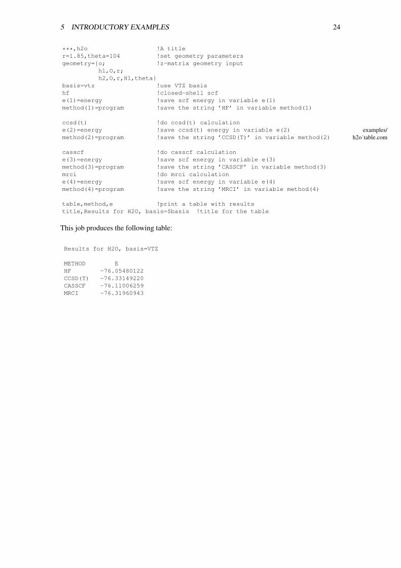
5 INTRODUCTORY EXAMPLES 24
***,h2o !A titler=1.85,theta=104 !set geometry parametersgeometry={o; !z-matrix geometry input
h1,O,r;h2,O,r,H1,theta}
basis=vtz !use VTZ basishf !closed-shell scfe(1)=energy !save scf energy in variable e(1)method(1)=program !save the string ’HF’ in variable method(1)
ccsd(t) !do ccsd(t) calculatione(2)=energy !save ccsd(t) energy in variable e(2)method(2)=program !save the string ’CCSD(T)’ in variable method(2)
casscf !do casscf calculatione(3)=energy !save scf energy in variable e(3)method(3)=program !save the string ’CASSCF’ in variable method(3)mrci !do mrci calculatione(4)=energy !save scf energy in variable e(4)method(4)=program !save the string ’MRCI’ in variable method(4)
table,method,e !print a table with resultstitle,Results for H2O, basis=$basis !title for the table
examples/h2o˙table.com
This job produces the following table:
Results for H2O, basis=VTZ
METHOD EHF -76.05480122CCSD(T) -76.33149220CASSCF -76.11006259MRCI -76.31960943

5 INTRODUCTORY EXAMPLES 25
5.7 Procedures
You could simplify this job by defining a procedure SAVE E as follows:
! $Revision: 2006.0 $
***,h2o !A title
proc save_e !define procedure save_eif(#i.eq.0) i=0 !initialize variable i if it does not existi=i+1 !increment ie(i)=energy !save scf energy in variable e(i)method(i)=program !save the present method in variable method(i)endproc !end of procedure
r=1.85,theta=104 !set geometry parametersgeometry={o; !z-matrix geometry input
h1,O,r;h2,O,r,H1,theta}
basis=vtz !use VTZ basishf !closed-shell scfsave_e !call procedure, save results
ccsd(t) !do ccsd(t) calculationsave_e !call procedure, save results
casscf !do casscf calculationsave_e !call procedure, save results
mrci !do mrci calculationsave_e !call procedure, save results
table,method,e !print a table with resultstitle,Results for H2O, basis=$basis !title for the table
examples/h2o˙proce.com
The job produces the same table as before. If you put the procedure SAVE E in afile molproi.rc or $HOME/.molproirc, it would be automatically included in allyour jobs (./molproi.rc is searched first; if this file does not exist, molpro looks for$HOME/.molproirc. If this also does not exist, molpro uses the default file in the systemdirectory).
5.8 Do loops
Now you have the idea that one geometry is not enough. Why not compute the whole surface?DO loops make it easy. Here is an example, which computes a whole potential energy surfacefor H2O.

5 INTRODUCTORY EXAMPLES 26
! $Revision: 2006.0 $
***,H2O potentialgeometry={x; !use cs symmetry
o; !z-matrixh1,o,r1(i);h2,o,r2(i),h1,theta(i) }
basis=vdz !define basis setangles=[100,104,110] !list of anglesdistances=[1.6,1.7,1.8,1.9,2.0] !list of distancesi=0 !initialize a counterdo ith=1,#angles !loop over all angles H1-O-H2do ir1=1,#distances !loop over distances for O-H1do ir2=1,ir1 !loop over O-H2 distances(r1.ge.r2)i=i+1 !increment counterr1(i)=distances(ir1) !save r1 for this geometryr2(i)=distances(ir2) !save r2 for this geometrytheta(i)=angles(ith) !save theta for this geometryhf; !do SCF calculationescf(i)=energy !save scf energy for this geometryccsd(t); !do CCSD(T) calculationeccsd(i)=energc !save CCSD energyeccsdt(i)=energy !save CCSD(T) energyenddo !end of do loop ithenddo !end of do loop ir1enddo !end of do loop ir2{table,r1,r2,theta,escf,eccsd,eccsdt !produce a table with resultshead, r1,r2,theta,scf,ccsd,ccsd(t) !modify column headers for tablesave,h2o.tab !save the table in file h2o.tabtitle,Results for H2O, basis $basis !title for tablesort,3,1,2} !sort table
examples/h2o˙pes˙ccsdt.com
This produces the following table.
Results for H2O, basis VDZ
R1 R2 THETA SCF CCSD CCSD(T)1.6 1.6 100.0 -75.99757338 -76.20140563 -76.204039201.7 1.6 100.0 -76.00908379 -76.21474489 -76.217475821.7 1.7 100.0 -76.02060127 -76.22812261 -76.23095473...2.0 1.9 110.0 -76.01128923 -76.22745359 -76.230819682.0 2.0 110.0 -76.00369171 -76.22185092 -76.22537212
You can use also use DO loops to repeat your input for different methods.
! $Revision: 2006.0 $
***,h2o benchmark$method=[hf,fci,ci,cepa(0),cepa(1),cepa(2),cepa(3),mp2,mp3,mp4,\
qci,ccsd,bccd,qci(t),ccsd(t),bccd(t),casscf,mrci,acpf]basis=dz !Double zeta basis setgeometry={o;h1,o,r;h2,o,r,h1,theta} !Z-matrix for geometryr=1 ang, theta=104 !Geometry parametersdo i=1,#method !Loop over all requested methods$method(i); !call programe(i)=energy !save energy for this methodenddoescf=e(1) !scf energyefci=e(2) !fci energytable,method,e,e-escf,e-efci !print a table with results!Title for table:title,Results for H2O, basis $basis, R=$r Ang, Theta=$theta degree
examples/h2o˙manymethods.com
This calculation produces the following table.

5 INTRODUCTORY EXAMPLES 27
Results for H2O, basis DZ, R=1 Ang, Theta=104 degree
METHOD E E-ESCF E-EFCIHF -75.99897339 .00000000 .13712077FCI -76.13609416 -.13712077 .00000000CI -76.12844693 -.12947355 .00764722CEPA(0) -76.13490643 -.13593304 .00118773CEPA(1) -76.13304720 -.13407381 .00304696CEPA(2) -76.13431548 -.13534209 .00177868CEPA(3) -76.13179688 -.13282349 .00429728MP2 -76.12767140 -.12869801 .00842276MP3 -76.12839400 -.12942062 .00770015MP4 -76.13487266 -.13589927 .00122149QCI -76.13461684 -.13564345 .00147732CCSD -76.13431854 -.13534515 .00177561BCCD -76.13410586 -.13513247 .00198830QCI(T) -76.13555640 -.13658301 .00053776CCSD(T) -76.13546225 -.13648886 .00063191BCCD(T) -76.13546100 -.13648762 .00063315CASSCF -76.05876129 -.05978790 .07733286MRCI -76.13311835 -.13414496 .00297580ACPF -76.13463018 -.13565679 .00146398
One can do even more fancy things, like, for instance, using macros, stored as string variables.See example oh macros.com for a demonstration.

6 PROGRAM CONTROL 28
6 PROGRAM CONTROL
6.1 Starting a job (***)
The first card of each input should be:
***,text
where text is arbitrary. If file 1 is restarted, text must always be the same. The effect of this cardis to reset all program counters, etc. If the *** card is omitted, text assumes its default value,which is all blank.
6.2 Ending a job (---)
The end of the input is signaled by either an end of file, or a
---
card. All input following the --- card is ignored.
Alternatively, a job can be stopped at at some place by inserting an EXIT card. This could alsobe in the middle of a DO loop or an IF block. If in such a case the --- card would be used, anerror would result, since the ENDDO or ENDIF cards would not be found.
6.3 Restarting a job (RESTART)
In contrast to MOLPRO92 and older versions, the current version of MOLPRO attempts to recoverall information from all permanent files by default. If a restart is unwanted, the NEW option canbe used on the FILE directive. The RESTART directive as described below can still be used asin MOLPRO92, but is usually not needed.
RESTART,r1,r2,r3,r4, . . .;
The ri specify which files are restarted. These files must have been allocated before using FILEcards. There are two possible formats for the ri:
a) 0 < ri < 10: Restart file ri and restore all information.
b) ri = name.nr: Restart file nr but truncate before record name.
If all ri = 0, then all permanent files are restarted. However, if at least one ri is not equal to zero,only the specified files are restarted.
Examples:
RESTART; will restart all permanent files allocated with FILE cards (default)
RESTART,1; will restart file 1 only
RESTART,2; will restart file 2 only
RESTART,1,2,3; will restart files 1-3
RESTART,2000.1; will restart file 1 and truncate before record 2000.

6 PROGRAM CONTROL 29
6.4 Including secondary input files (INCLUDE)
INCLUDE,file,echo;
Insert the contents of the specified file in the input stream. In most implementations the filename given is used directly in a Fortran open statement. If the parameter echo is nonzero, theincluded file is echoed to the output in the normal way, but by default its contents are not printed.The included file may itself contain INCLUDE commands up to a maximum nesting depth of10.
6.5 Allocating dynamic memory (MEMORY)
MEMORY,n,scale;
Sets the limit on dynamic memory to n floating point words. If scale is given as K, n is multipliedby 1000; if scale is M, n is multiplied by 1 000 000.
Note: The MEMORY card must precede all FILE cards!
Examples:
MEMORY,90000 allocates 90 000 words of memory
MEMORY,500,K allocates 500 000 words of memory
MEMORY,2,M allocates 2 000 000 words of memory
6.6 DO loops (DO/ENDDO)
DO loops can be constructed using the DO and ENDDO commands. The general format of the DOcommand is similar to Fortran:
DO variable=start, end [[,]increment] [[,]unit]
where start, end, increment may be expressions or variables. The default for increment is 1. Incontrast to Fortran, these variables can be modified within the loop (to be used with care!). Forinstance:
DR=0.2DO R=1.0,6.0,DR,ANGIF (R.EQ.2) DR=0.5IF (R.EQ.3) DR=1.0....ENDDO
performs the loop for the following values of R: 1.0, 1.2, 1.4, 1.6, 1.8, 2.0,2.5, 3.0, 4.0, 5.0, 6.0 Angstrøm. The same could be achieved as follows:
RVEC=[1.0,1.2,1.4,1.6,1.8,2.0,2.5,3.0,4.0,5.0,6.0] ANGDO I=1,#RVECR=RVEC(I)....ENDDO
Up to 20 DO loops may be nested. Each DO must end with its own ENDDO.
Jumps into DO loops are possible if the DO variables are known. This can be useful in restarts,since it allows to continue an interrupted calculation without changing the input (all variablesare recovered in a restart).

6 PROGRAM CONTROL 30
6.6.1 Examples for do loops
The first example shows how to compute a potential energy surface for water.
! $Revision: 2006.0 $
***,H2O potentialgeometry={x; !use cs symmetry
o; !z-matrixh1,o,r1(i);h2,o,r2(i),h1,theta(i) }
basis=vdz !define basis setangles=[100,104,110] !list of anglesdistances=[1.6,1.7,1.8,1.9,2.0] !list of distancesi=0 !initialize a counterdo ith=1,#angles !loop over all angles H1-O-H2do ir1=1,#distances !loop over distances for O-H1do ir2=1,ir1 !loop over O-H2 distances(r1.ge.r2)i=i+1 !increment counterr1(i)=distances(ir1) !save r1 for this geometryr2(i)=distances(ir2) !save r2 for this geometrytheta(i)=angles(ith) !save theta for this geometryhf; !do SCF calculationescf(i)=energy !save scf energy for this geometryccsd(t); !do CCSD(T) calculationeccsd(i)=energc !save CCSD energyeccsdt(i)=energy !save CCSD(T) energyenddo !end of do loop ithenddo !end of do loop ir1enddo !end of do loop ir2{table,r1,r2,theta,escf,eccsd,eccsdt !produce a table with resultshead, r1,r2,theta,scf,ccsd,ccsd(t) !modify column headers for tablesave,h2o.tab !save the table in file h2o.tabtitle,Results for H2O, basis $basis !title for tablesort,3,1,2} !sort table
examples/h2o˙pes˙ccsdt.com
The next example shows how to loop over many methods.
! $Revision: 2006.0 $
***,h2o benchmark$method=[hf,fci,ci,cepa(0),cepa(1),cepa(2),cepa(3),mp2,mp3,mp4,\
qci,ccsd,bccd,qci(t),ccsd(t),bccd(t),casscf,mrci,acpf]basis=dz !Double zeta basis setgeometry={o;h1,o,r;h2,o,r,h1,theta} !Z-matrix for geometryr=1 ang, theta=104 !Geometry parametersdo i=1,#method !Loop over all requested methods$method(i); !call programe(i)=energy !save energy for this methodenddoescf=e(1) !scf energyefci=e(2) !fci energytable,method,e,e-escf,e-efci !print a table with results!Title for table:title,Results for H2O, basis $basis, R=$r Ang, Theta=$theta degree
examples/h2o˙manymethods.com
6.7 Branching (IF/ELSEIF/ENDIF)
IF blocks and IF/ELSEIF blocks can be constructed as in FORTRAN.
6.7.1 IF statements
IF blocks have the same form as in Fortran:

6 PROGRAM CONTROL 31
IF (logical expression) THENstatementsENDIF
If only one statement is needed, the one-line form
IF (logical expression) statement
can be used, except if statement is a procedure name.
ELSE and ELSE IF can be used exactly as in Fortran. IF statements may be arbitrarily nested.Jumps into IF or ELSE IF blocks are allowed. In this case no testing is performed; when anELSE is reached, control continues after ENDIF.
The logical expression may involve logical comparisons of algebraic expressions or of strings.Examples:
IF(STATUS.LT.0) THENTEXT,An error occurred, calculation stoppedSTOPENDIF
IF($method.eq.’HF’) then...ENDIF
In the previous example the dollar and the quotes are optional:
IF(METHOD.EQ.HF) then...ENDIF
6.7.2 GOTO commands
GOTO commands can be used to skip over parts of the input. The general form is
GOTO,command,[n],[nrep]
Program control skips to the |n|’th occurrence of command (Default: n = 1). command must bea keyword in the first field of an input line. If n is positive, the search is forward starting fromthe current position. If n is negative, search starts from the top of the input. The GOTO commandis executed at most nrep times. The default for nrep is 1 if n < 0 and infinity otherwise. Werecommend that GOTO commands are never used to construct loops.
Alternatively, one can jump to labels using
GOTO,label
Since labels must be unique, the search starts always from the top of the input. It is required thatthe label ends with a colon.
6.7.3 Labels (LABEL)
LABEL
This is a dummy command, sometimes useful in conjunction with GOTO.

6 PROGRAM CONTROL 32
6.8 Procedures (PROC/ENDPROC)
Procedures can be defined at the top of the input, in the default file molproi.rc, or inINCLUDE files as follows:
PROC namestatementsENDPROC
Alternatively, one can use the form
PROC name[=]{statements}
In the latter case, it is required that the left curly bracket ({) appears on the same line as PROC,but statements can consist of several lines. If in the subsequent input name is found as a com-mand in the first field of a line, it is substituted by the statements. Example:
PROC SCFIF (#SPIN.EQ.0.OR.MOD(SPIN,2).NE.MOD(NELEC,2)) SET,SPIN=MOD(NELEC,2)IF (SPIN.EQ.0) THENHF
ELSERHF
ENDIFENDPROC
Alternatively, this could be written as
PROC SCF={IF (#SPIN.EQ.0.OR.MOD(SPIN,2).NE.MOD(NELEC,2)) SET,SPIN=MOD(NELEC,2)IF (SPIN.EQ.0) THEN; HF; ELSE; RHF; ENDIF}
Procedures may be nested up to a depth of 10. In the following example SCF is a procedure:
PROC CCSCFIF (SPIN.EQ.0) THENCCSD
ELSERCCSD
ENDPROC
Note: Procedure names are substituted only if found in the first field of an input line. Therefore,they must not be used on one-line IF statements; please use IF / ENDIF structures instead.
If as first statement of a procedure ECHO is specified, the substituted commands of the presentand lower level procedures will be printed. If ECHO is specified in the main input file, allsubsequent procedures are printed.
Certain important input data can be passed to the program using variables. For instance, occu-pancy patterns, symmetries, number of electrons, and multiplicity can be defined in this way(see section 8.8 for more details). This allows the quite general use of procedures. For example,assume the following procedure has been defined in molproi.rc:
PROC MRCIIF (INTDONE.EQ.0) INTIF (SCFDONE.EQ.0) THENSCF

6 PROGRAM CONTROL 33
ENDIFMULTICIENDPROC
This procedure can be used for a calculation of a vertical ionization potential of H2O as follows:
R=1 ANG !Set bond distanceTHETA=104 DEGREE !Set bond angle
BASIS=VTZ !Define basis set
GEOMETRY !Geometry input blockO !Z-matrixH1,O,RH2,O,R,H1,THETAENDG !End of geometry inputHFMRCI !Compute mrci energy of water using defaultsEH2O=ENERGY !save mrci energy in variable EH2O
SET,NELEC=9 !Set number of electrons to 9SET,SYMMETRY=2 !Set wavefunction symmetry to 2HFMRCI !Compute mrci energy of H2O+ (2B2 state)
IPCI=(ENERGY-EH2O)*TOEV !Compute MRCI ionization potential in eV
Note: At present, all variables are global, i.e., variables are commonly known to all proceduresand all variables defined in procedures will be subsequently known outside the procedures aswell. The reason is that procedures are included into the internal input deck at the beginning ofthe job and not at execution time; for the same reason, variable substitution of procedure namesis not possible, e.g. one cannot use constructs like
method=scf$method !this does not work!
6.9 Text cards (TEXT)
TEXT,xxxxxx
will just print xxxxxx in the output. If the text contains variables which are preceded by a dollar($), these are replaced by their actual values, e.g.
r=2.1text,Results for R=\$r
will print
Results for R=2.1
6.10 Checking the program status (STATUS)
STATUS,[ALL|LAST|commands],[IGNORE|STOP|CRASH],[CLEAR]

6 PROGRAM CONTROL 34
This command checks and prints the status of the specified program steps. commands may bea list of commands for wavefunction calculations previously executed in the current job. If nocommand or LAST is specified, the status of the last step is checked. If ALL is given, all programsteps are checked.
If CRASH or STOP is given, the program will crash or stop, respectively, if the status was noto.k. (STOP is default). If IGNORE is given, any bad status is ignored. If CLEAR is specified,all status information for the checked program steps is erased, so there will be no crash atsubsequent status checks.
Examples:
STATUS,HF,CRASH; will check the status of the last HF-SCF step and crash if it was noto.k. (i.e. no convergence). CRASH is useful to avoid that the nextprogram in a chain is executed.
STATUS,MULTI,CI,STOP; will check the status of the most previous MULTI and CI stepsand stop if something did not converge.
STATUS,RHF,CLEAR; will clear the status flag for last RHF. No action even if RHF did notconverge.
Note that the status variables are not recovered in a restart.
By default, the program automatically does the following checks:
1.) If an orbital optimization did not converge, and the resulting orbitals are used in a subse-quent correlation calculation, an error will result. This the error exit can be avoided using theIGNORE ERROR option on the ORBITAL directive.
2.) If a CCSD|QCI|BCC|LMPn calculation did not converge, further program steps which dependon the solution (e.g, Triples, CPHF, EOM) will not be done and an error will result. This can beavoided using the NOCHECK option on the command line.
3.) In geometry optimizations or frequency calculations no convergence will lead to immediateerror exits.
6.11 Global Thresholds (GTHRESH)
A number of global thresholds can be set using the GTHRESH command outside the individualprograms (the first letter G is optional, but should be used to avoid confusion with programspecific THRESH cards). The syntax is
GTHRESH,key1=value1,key2=value2,. . .
key can be one of the following.
ZERO Numerical zero (default 1.d-12)
ONEINT Threshold for one-electron integrals (default 1.d-12, but not used atpresent)
TWOINT Threshold for the neglect of two-electron integrals (default 1.d-12)
PREFAC Threshold for test of prefactor in TWOINT (default 1.d-14)
LOCALI Threshold for orbital localization (default 1.d-8)
EORDER Threshold for reordering of orbital after localization (default 1.d-4)

6 PROGRAM CONTROL 35
ENERGY Convergence threshold for energy (default 1.d-6)
GRADIENT Convergence threshold for orbital gradient in MCSCF (default 1.d-2)
STEP Convergence threshold for step length in MCSCF orbital optimization(default 1.d-3)
ORBITAL Convergence threshold for orbital optimization in the SCF program(default 1.d-5).
CIVEC Convergence threshold for CI coefficients in MCSCF and referencevector in CI (default 1.-d.5)
COEFF Convergence threshold for coefficients in CI and CCSD(default 1.d-4)
PRINTCI Threshold for printing CI coefficients (default 0.05)
PUNCHCI Threshold for punching CI coefficients (default 99 - no punch)
SYMTOL Threshold for finding symmetry equivalent atoms (default 1.d-6)
GRADTOL Threshold for symmetry in gradient (default 1.d-6).
THROVL Threshold for smallest allowed eigenvalue of the overlap matrix (de-fault 1.d-8)
THRORTH Threshold for orthonormality check (default 1.d-8)
6.12 Global Print Options (GPRINT/NOGPRINT)
Global print options can be set using the GPRINT command outside the individual programs(the first letter G is optional, but should be used to avoid confusion with program specific PRINTcards). The syntax is
GPRINT,key1[=value1],key2[=value2],. . .NOGPRINT,key1,key2,. . .
Normally, value can be omitted, but values > 0 may be used for debugging purposes, givingmore information in some cases. The default is no print for all options, except for DISTANCE,ANGLES (default=0), and VARIABLE. NOGPRINT,key is equivalent to PRINT,key=-1. keycan be one of the following:
BASIS Print basis information
DISTANCE Print bond distances (default)
ANGLES Print bond angle information (default). If > 0, dihedral angles arealso printed.
ORBITAL Print orbitals in SCF and MCSCF
CIVECTOR Print CI vector in MCSCF
PAIRS Print pair list in CI, CCSD
CS Print information for singles in CI, CCSD
CP Print information for pairs in CI, CCSD
REF Print reference CSFs and their coefficients in CI
PSPACE Print p-space configurations
MICRO Print micro-iterations in MCSCF and CI
CPU Print detailed CPU information

6 PROGRAM CONTROL 36
IO Print detailed I/O information
VARIABLE Print variables each time they are set or changed (default).
6.13 One-electron operators and expectation values (GEXPEC)
The operators for which expectation values are requested, are specified by keywords on theglobal GEXPEC directive. The first letter G is optional, but should be used to avoid confusionwith program specific EXPEC cards, which have the same form as GEXPEC. For all operatorsspecified on the GEXPEC card, expectation values are computed in all subsequent programs (ifapplicable).
For a number of operators it is possible to use generic operator names, e.g., DM for dipole mo-ments, which means that all three components DMX, DMY, and DMZ are computed. Alternatively,individual components may be requested.
The general format is as follows:
[G]EXPEC,opname[,][icen,[x,y,z]],...
where
opname operator name (string), either generic or component.
icen z-matrix row number or z-matrix symbol used to determine the origin(x,y,z must not be specified).If icen= 0 or blank, the origin must be specified in x,y,z
Several GEXPEC cards may follow each other, or several operators may be specified on onecard.
Examples:
GEXPEC,QM computes quadrupole moments with origin at (0,0,0),
GEXPEC,QM1 computes quadrupole moments with origin at centre 1.
GEXPEC,QM,O1 computes quadrupole moments with origin at atom O1.
GEXPEC,QM,,1,2,3 computes quadrupole moments with origin at (1,2,3).
The following table summarizes all available operators:
Expectation values are only nonzero for symmetric operators (parity=1). Other operators can beused to compute transition quantities (spin-orbit operators need a special treatment). By default,the dipole moments are computed.
6.13.1 Example for computing expectation values
The following job computes dipole and quadrupole moments for H2O.

6 PROGRAM CONTROL 37
! $Revision: 2006.0 $
***,h2o propertiesgeometry={o;h1,o,r;h2,o,r,h1,theta} !Z-matrix geometry inputr=1 ang !bond lengththeta=104 !bond anglegexpec,dm,sm,qm !compute dipole and quarupole moments$methods=[hf,multi,ci] !do hf, casscf, mrcido i=1,#methods !loop over methods$methods(i) !run energy calculatione(i)=energydip(i)=dmz !save dipole moment in variable dipquadxx(i)=qmxx !save quadrupole momemtsquadyy(i)=qmyyquadzz(i)=qmzzsmxx(i)=xx !save second momemtssmyy(i)=yysmzz(i)=zzenddotable,methods,dip,smxx,smyy,smzz !print table of first and second momentstable,methods,e,quadxx,quadyy,quadzz !print table of quadrupole moments
examples/h2o˙gexpec2.com
This Job produces the following tables
METHODS DIP SMXX SMYY SMZZHF 0.82747571 -5.30079792 -3.01408114 -4.20611391MULTI 0.76285513 -5.29145148 -3.11711397 -4.25941000CI 0.76868508 -5.32191822 -3.15540500 -4.28542917
METHODS E QUADXX QUADYY QUADZZHF -76.02145798 -1.69070039 1.73937477 -0.04867438MULTI -76.07843443 -1.60318949 1.65831677 -0.05512728CI -76.23369821 -1.60150114 1.64826869 -0.04676756
6.13.2 Example for computing relativistic corrections
***,ar2geometry={ar1;ar2,ar1,r} !geometry definitionr=2.5 ang !bond distance{hf; !non-relativisitic scf calculationexpec,rel,darwin,massv} !compute relativistic correction using Cowan-Griffin operatore_nrel=energy !save non-relativistic energy in variable enrelshow,massv,darwin,erel !show individual contribution and their sum
dkroll=1 !use douglas-kroll one-electron integralshf; !relativistic scf calculatione_dk=energy !save relativistic scf energy in variable e_dk.show,massv,darwin,erel !show mass-velocity and darwin contributions and their sumshow,e_dk-e_nrel !show relativistic correction using Douglas-Kroll
examples/ar2˙rel.com
This jobs shows at the end the following variables:
MASSV / AU = -14.84964285DARWIN / AU = 11.25455679EREL / AU = -3.59508606

6 PROGRAM CONTROL 38
Table 5: One-electron operators and their componentsGeneric Parity Components DescriptionnameOV 1 OverlapEKIN 1 Kinetic energyPOT 1 potential energyDELT 1 delta functionDEL4 1 ∆4
DARW 1 one-electron Darwin term,i.e., DELT with appropriate factorssummed over atoms.
MASSV 1 mass-velocity term,i.e., DEL4 with appropriate factor.
REL 1 total Cowan-Griffin Relativistic correction,i.e., DARW+MASSV.
DM 1 DMX, DMY, DMZ dipole momentsSM 1 XX, YY, ZZ, XY, XZ, YZ second momentsTM 1 XXX, XXY, XXZ, XYY, XYZ,
XZZ, YYY, YYZ, YZZ, ZZZ third momentsMLTPn 1 all unique Cartesian products of order n multipole momentsQM 1 QMXX, QMYY, QMZZ, QMXY, QMXZ, QMYZ, quadrupole moments and R2
QMRR=XX + YY + ZZ,QMXX=(3 XX - RR)/2,QMXY=3 XY / 2 etc.
EF 1 EFX, EFY, EFZ electric fieldFG 1 FGXX, FGYY, FGZZ, FGXY, FGXZ, FGYZ electric field gradientsDMS 1 DMSXX, DMSYX, DMSZX,
DMSXY, DMSYY, DMSZY,DMSXZ, DMSYZ, DMSZZ diamagnetic shielding tensor
LOP -1 LX, LY, LZ Angular momentum operators Lx, Ly, Lz
LOP2 1 LXLX, LYLY, LZLZ, one electron parts of products ofLXLY, LXLZ, LYLZ angular momentum operators.The symmetric combinations 1
2(LxLy + LyLx) etc. are computedVELO -1 D/DX, D/DY, D/DZ velocityLS -1 LSX, LSY, LSZ spin-orbit operatorsECPLS -1 ECPLSX, ECPLSY, ECPLSZ ECP spin-orbit operators

7 FILE HANDLING 39
7 FILE HANDLING
7.1 FILE
The FILE directive is used to open permanent files, which can be used for later restarts. Thesyntax in MOLPRO94 and later versions is
FILE,file,name,[status]
file is the logical MOLPRO file number (1-9). name is the file name (will be converted to lowercase). status can be one of the following:
UNKNOWN A permanent file is opened. If it exists, it is automatically restarted.This is the default.
OLD Same effect as UNKNOWN. No error occurs if the file does not exist.
NEW A permanent file is opened. If it already exists, it is erased and notrestarted.
ERASE Same effect as NEW.
SCRATCH A temporary file is opened. If it already exists, it is erased and notrestarted. After the job has finished, the file is no longer existent.
DELETE Same effect as SCRATCH.
Note that RESTART is now the default for all permanent files. All temporary files are usuallyallocated automatically where needed. I/O buffers are allocated at the top of the dynamic mem-ory, and the available memory decreases by the size of the buffers. The MEMORY card musttherefore be presented before the first FILE card!
Examples:
FILE,1,H2O.INT allocates permanent file 1 with name H2O.INT. Previous informationon the file is recovered.
FILE,2,H2O.WFU,NEW allocates permanent file 2 with name H2O.WFU. All previous infor-mation on the file is erased.
Note that filenames are converted to lower case on unix machines.
7.2 DELETE
DELETE,file1, file2, . . .
Deletes the specified files. file refers to the logical MOLPRO file numbers as specified on theFILE card.
7.3 ERASE
ERASE,file1, file2, . . .
Erases the specified files. file refers to the logical MOLPRO file numbers as specified on theFILE card.

7 FILE HANDLING 40
7.4 DATA
The DATA command can be used to modify the MOLPRO binary files.
UNIT Alias for NPL (should never be used)
RENAME,rec1,rec2 used to rename rec1 to rec2. rec1 and rec2 must be given in the formname.ifil, where ifil is the number of a MOLPRO binary file (alias forNAME).
TRUNCATE,nen used to truncate files after nen-1 records (alias for NEN).
TRUNCATE,rec used to truncate before record rec. rec must be given in the formname.ifil, where ifil is the number of a MOLPRO binary file.
COUNT Alias for NRE (presently not used)
COPY,rec1,rec2 Copies record rec1 to rec2. rec1 and rec2 must be given in the formnam1.ifil1, nam2.ifil2. If nam2=0, nam2=nam1. If nam1=0, all recordsare copied from file ifil1 to file ifil2.
7.5 Assigning punch files (PUNCH)
PUNCH,filename,[REWIND]
Opens punch file named filename. If this file already exists, it is appended, unless the REWINDor NEW option is specified; in that case, any previous information on the punch file is overwrit-ten. See FILE for machine dependent interpretation of filename. The punch file contains allimportant results (geometries, energies, dipole, transition moments etc). It can be read by aseparate program READPUN, which can produce tables in user supplied format.
Example:
PUNCH,H2O.PUN allocates punch file H2O.PUN
Note that the file name is converted to lower case on unix machines.
7.6 MOLPRO system parameters (GPARAM)
The GPARAM card allows to change MOLPRO system parameters. This should only be usedby experts!
GPARAM,option=value,. . .
The following options can be given in any order.
NOBUFF if present, disable system buffering
LSEG disk sector length
INTREL number of integer words per real word (should never be modified!)
IBANK number of memory banks. Default is 2, which should always be o.k.
IVECT 0=scalar, 1=vector machine
MINVEC minimum vector length for call to mxmb
LTRACK page size in buffer routines (must be multiple of lseg)

8 VARIABLES 41
LENBUF length of integral buffer (file 1)
NTR length of integral records (must be multiple of 3·ltrack)
LTR disk sector length assumed in CI (default 1 is reasonable)
NCACHE machine cache size in bytes
IASYN if nonzero, use asynchronous I/O on CONVEX
MXMBLK column/row block size for mxma
MXMBLN link block size for mxma
NCPUS maximum number of cpus to be used in multitasking
MINBR1 min number of floating point ops per processor
MXDMP highest file number to be treated as dump file with full functionality (1 ≤ .MXDMP≤ .3).
The MXDMP option is for experts only! This prevents basis and geometry information frombeing written to dump files with higher file number than the given value, and can sometimes beuseful for counterpoise corrected geometry optimizations. Note that some functionality is lostby giving this option, and errors will result unless all input is correct!
8 VARIABLES
Data may be stored in variables. A variable can be of type string, real or logical, depending onthe type of the expression in its definition. Any sequence of characters which is not recognizedas expression or variable is treated as string. In this section, we will discuss only real and logicalvariables. String variables will be discussed in more detail in section 8.3. Variables can be usedanywhere in the input, but they can be set only outside the input blocks for specific programs.For example, if a variable is used within the input block for HF, it must have been set before theHF{...} input block.
MOLPRO automatically stores various results and data in system variables (see section 8.8.1),which can be used for further processing. A new feature of MOLPRO2002 is that most systemvariables are write protected and cannot be overwritten by the user. The input is automaticallychecked before the job starts, and should a system variable be set in the input the job will stopimmediately with an error message. Only in some exceptions (see section 8.4), system variablescan be modified using the SET command (but not with the simple NAME=value syntax). Notethat due to the changed usage and syntax of the SET command, compatibility with MOLPRO92input syntax is no longer maintained.
8.1 Setting variables
A variable can be defined using
variable1=value1, variable2=value2, . . .
A variable definition is recognized by the equals sign in the first field of the input card. Forexample,
THRESH,ENERGY=1.d-8,GRADIENT=1.d-5
does not define variables; here ENERGY and GRADIENT are options for the THRESH directive.
Variables can have different types:

8 VARIABLES 42
Numbers: The value is a number or an expression. The general form of value isexpression [,] [unit]unit is an optional string which can be used to associate a unit to the value.ANG[STROM], DEGREE, HARTREE are examples. Undefined variables inexpressions are assumed to be zero (and defined to be zero at the same time).
Logicals: The value can be .TRUE. or .FALSE. (.T. and .F. also work), or a logicalexpression. Internally, .TRUE. is stored as 1 and .FALSE. as zero.
Strings: The value can either be a string enclosed in quotes or a string variable. Seesection 8.3 for more details.
8.2 Indexed variables
Variables can be indexed, but only one-dimensional indexing is available. Indexed variables canbe defined either individually, e.g.
R(1)=1.0 ANGR(2)=1.2 ANGR(3)=1.3 ANG
or as a vector of values enclosed by square brackets:
R=[1.0,1.1,1.2] ANG
Subranges can also be defined, e.g.
R(1)=1.0 ANGR(2:3)=[1.1,1.2] ANG
leads to the same result as the above two forms.
The type of each element depends on the type of the assigned value, and it is possible to mixtypes in one variable. Example:
geometry={he}hfresult=[program,energy,status.gt.0]
yields:
RESULT(1) = HF-SCFRESULT(2) = -2.85516048 AURESULT(3) = TRUE
In this example the variables PROGRAM, ENERGY, and STATUS are system variables, whichare set by the program (see section 8.4).

8 VARIABLES 43
8.3 String variables
As explained already in section 8.1, string variables can be set as other variables in the form
variable = ’string’variable = string variable
Strings must be enclosed by quotes. Otherwise the string is assumed to be a variable, and if thisis undefined it is assumed to be zero.
Alternatively, if the name of the variable is preceded by a dollar ($), all values is assumed to bea string. This can a string variable, a quoted string, or an unquoted string. Note that unquotedstrings are converted to upper case. Also note that quotes are compulsory if the string containsblanks.
Example:
$str=[a,b+4,’This is an example for strings’]
yields
STR(1) = ASTR(2) = B+4STR(3) = This is an example for strings
As a general rule, string variables are replaced by their value only if they are preceded by adollar ($) (exceptions: in variable definitions, on SHOW cards, and in logical expressions on IFcards, the dollar is optional). This is a precaution to avoid commands which have the same nameas a variable being interpreted as variables. Variables may also appear on TEXT or TITLE cardsor in strings, but must be preceded by $ in these cases. Example:
$METHOD=MCSCFR=1.5TEXT,$method results for R=$R Bohr
prints
MCSCF results for R=1.5 Bohr
String variables can be concatenated with strings or other string variables in the following way.Assume that variable PROGRAM has the value MRCI. Setting
METHOD=’$PROGRAM+Q’
sets METHOD to MRCI+Q. Alternatively, if we would also have a variable VERSION with valueQ, we could write
METHOD=’$PROGRAM+$VERSION’
Again, the value of METHOD would be MRCI+Q. Note that the quotes are necessary in thesecases.
Substring operations are not implemented.

8 VARIABLES 44
8.4 System variables
As mentioned above, most system variables cannot be written by the user. In some exceptions,it is possible to redefine them using the SET command:
SET,variable = expression [,] [unit]
This holds for the following variables:
CHARGE Total charge of the molecule
NELEC Number of electrons
SPIN Spin quantum number, given as 2 ·M S (integer)
SCFSPIN Same as SPIN, but only for HF
MCSPIN Same as SPIN, but only for MCSCF
CISPIN Same as SPIN, but only for MRCI
STATE State to be optimized
MCSTATE Same as STATE but only for MCSCF
CISTATE Same as STATE but only for MRCI
SYMMETRY State symmetry
SCFSYM[METRY] Same as SYMMETRY but only for HF
MCSYM[METRY] Same as SYMMETRY but only for MCSCF
CISYM[METRY] Same as SYMMETRY but only for MRCI
ZSYMEL Symmetry elements
LQUANT Lambda quantum number for linear molecules
OPTCONV Geometry optimization convergence criterion
PROGRAM Last program name
CPUSTEP CPU-time of last program step
SYSSTEP System-time of last program step
WALLSTEP Elapsed-time of last program step
FOCKDONE Indicates if closed-shell fock operator is available.
8.5 Macro definitions using string variables
String variables for which the stored string has the form of an algebraic expression are evaluatedto a number if they are preceded by two dollars ($$). Example:
string=’a+b’a=3b=4text,This is string $string which evaluates to $$string
prints
** This is string a+b which evaluates to 7
This can be used to define simple macros, which can be used at various places in the subsequentinput. For instance,

8 VARIABLES 45
ECORR=’ENERGY-ESCF’ !define a macroHF !do SCF calculationESCF=ENERGY !store SCF energy in variable ESCFMULTI !do CASSCFDEMC=$$ECORR !store CASSCF correlation energy in variable DEMCMRCI !do MRCIDECI=$$ECORR !store MRCI correlation energy in variable DECI
Here is an example of advanced use of macros and string variables:
! $Revision: 2006.0 $
***,test for parsertext,This fancy input demonstrates how string variables and macros can be usedtextbasis=vdz !define basis setgeometry={O;H,O,r} !define geometry (z-matrix)
text,methods$method=[rhf,2[casscf,2[mrci]]]text,active spacesspaces=[’[3,1,1]’,3[’[4,2,2]’],3[’[5,2,2]’]]text,symmetriessymset=[’1’,2[’[1,2,3]’,’1’,’2’]]text,weight factors for state averaged casscfweights=[’1’,’[1,1,1]’,2[’ ’],’[1,0.5,0.5]’,2[’ ’]]text,scf occupationset,scfocc=[3,2[1]]text,bond distancer=1.85
hfdo i=1,#method !loop over methodsocc=$$spaces(i) !set active space for this runset,symmetry=$$symset(i) !set symmetries for this runset,weight=$$weights(i) !set weights for this run$method(i) !now run methode(i)=’$energy’ !save energies in stringsdipol(i)=’$dmz’ !save dipole moments in stringsenddotable,method,spaces,symset,weights,e,dipoltitle,Results for OH, r=$r, basis=$basishead,method,spaces,symmetries,weights,energies,’dipole moments’exit
examples/oh˙macros.com
8.6 Indexed Variables (Vectors)
Variables may be indexed, but only one-dimensional arrays (vectors) are supported. The indexmay itself be a variable. For instance
METHOD(I)=PROGRAME(I)=ENERGY
are valid variable definitions, provided I, PROGRAM, and ENERGY are also defined variables.Indices may be nested to any depth.
Different elements of an array can be of different type (either real or logical). However, onlyone unit can be assigned to an array. String variables have no associated value and cannot bemixed with the other variable types. Therefore, a given variable name can only be used eitherfor a string variable or a real (logical) variable.
Vectors (arrays) can be conveniently defined using square brackets:

8 VARIABLES 46
R=[1.0,1.2,1.3] ANG
This defines an array with three elements, which can be accessed using indices; for instance,R(2) has the value 1.2 ANG. A repeat specifier can be given in front of the left bracket: 5[0]is equivalent to [0,0,0,0,0]. Brackets can even be nested: for instance, 2[1,2,2[2.1,3.1]]is equivalent to [1,2,2.1,3.1,2.1,3.1,1,2,2.1,3.1,2.1,3.1].
Arrays can be appended from a given position just by entering additional elements; for instance,
R(4)=[1.4,1.5] ANG
or
R(4:)=[1.4,1.5] ANG
extends the above array to length 5. Previously defined values can be overwritten. For instance
R(2)=[1.25,1.35,1.45]
modifies the above vector to (1.0, 1.25, 1.35, 1.45, 1.5).
If no index is given on the left hand side of the equal sign, an existing variable of the same nameis replaced by the new values, and all old values are lost. For instance
THETA=[100,110,120,130] set four values
. . .
THETA(1)=104 replace THETA(1) by a new value; THETA(2:4) are unchanged
. . .
THETA=[140,150] old variable THETA is replaced; THETA(3:4) are deleted
Square brackets can also be used to define an array of strings, e.g.,
METHOD=[INT,HF,CASSCF,MRCI]
These could be used as follows:
DO I=1,4$METHOD(I)ENDDO
The above input would be equivalent to
INTHFCASSCFMRCI
The current length of an array can be accessed by preceding # to the variable name. For instance,in the above examples #R and #METHOD have the values 5 and 4, respectively. If a variable isnot defined, zero is returned but no error occurs. This can be used to test for the existence of avariable, for example:
IF(#SPIN.EQ.0.AND.#NELEC.EQ.1) SET,SPIN=MOD(NELEC,2)
This defines variable SPIN if it is unknown and if NELEC is a scalar (one dimensional) variable.

8 VARIABLES 47
8.7 Vector operations
The following simple vector operations are possible:
• Copying or appending a vector to another vector. For instance S=R copies a vector Rto a vector S. S(3)=R copies R to S(3), S(4), .... S(#S+1)=R appends vectorR to vector S. It is also possible to access a range of subsequent elements in a vector:S=R(2:4) copies elements 2 to 4 of R to S(1), S(2), S(3). Note that R(2:)denotes elements R(2) to R(#R), but R(2) denotes a single element of R.
• Vector-scalar operations: R=R*2multiplies each element of R by 2. Instead of the number2, also scalar (one dimensional) variables or expressions can be used, e.g., R=R*ANGconverts all elements of R from Angstrøm to bohr, or Z=R*COS(THETA) creates a vectorZ with elements Z(i) = R(i)*COS(THETA). All other algebraic operators can beused instead of “*”.
• Vector-vector operations: If A and B are vectors of the same length, then A × B is also avector of this length. Here × stands for any algebraic operator, and the operation is donefor each pair of corresponding elements. For instance, A + B adds the vectors A and B,and A * B multiplies their elements. Note that the latter case is not a scalar product. Ifan attempt is made to connect two vectors of different lengths by an algebraic operator,an error occurs.
• Intrinsic functions: Assume THETA=[100,110,120,-130] to be a vector of angles(in degrees). In this case X=2*COS(THETA) is also a vector containing the cosines ofeach element of THETAmultiplied by two, i.e., X(i) = 2*COS(THETA(i)). MAX(THETA)or MIN(THETA) return the maximum and minimum values, respectively, in array THETA.Vector operations can also be nested, e.g., MAX(ABS(THETA)) returns the maximumvalue in array ABS(THETA).
At present, vector operations are not supported with string variables.
8.8 Special variables
8.8.1 Variables set by the program
A number of variables are predefined by the program. The following variables can be used toconvert between atomic units and other units:
EV=1.d0/27.2113961d0 HARTREEKELVIN=1.d0/3.157733d5 HARTREEKJOULE=1.d0/2625.500d0 HARTREEKCAL=1.d0/627.5096d0 HARTREECM=1.d0/219474.63067d0 HARTREECM-1=1.d0/219474.63067d0 HARTREEHZ=1.d0/6.5796838999d15 HARTREEHERTZ=1.d0/6.5796838999d15 HARTREEANG=1.d0/0.529177249d0 BOHRANGSTROM=1.d0/0.529177249d0 BOHR
TOEV=27.2113961d0 EVTOK=3.157733d5 KTOKELVIN=3.157733d5 KTOCM=219474.63067d0 CM-1

8 VARIABLES 48
TOHERTZ=6.5796838999d15 HZTOHZ=6.5796838999d15 HZTOKJ=2625.500d0 KJ/MOLTOKJOULE=2625.500d0 KJ/MOLTOKCAL=627.5096d0 KCAL/MOLTOA=0.529177249d0 ANGSTROMTOANG=0.529177249d0 ANGSTROMTODEBYE=2.54158d0 DEBYE
Further variables which are set during execution of the program:
INTYP defines integral program to be used. Either INTS (Seward) or INTP(Argos).
INTDONE has the value .true. if the integrals are done for the current geom-etry.
CARTESIAN Set to one if Cartesian basis functions are used.
SCFDONE has the value .true. if an SCF calculation has been done for thecurrent geometry.
NUMVAR number of variables presently defined
STATUS status of last step (1=no error, -1=error or no convergence)
CHARGE Total charge of the molecule
NELEC number of electrons in last wavefunction
SPIN spin multiplicity minus one of last wavefunction
ORBITAL record of last optimized orbitals (set but never used in the program)
LASTORB Type of last optimized orbitals (RHF, UHF, UHFNAT, or MCSCF.
LASTSYM Symmetry of wavefunction for last optimized orbitals.
LASTSPIN 2∗MS for wavefunctions for last optimized orbitals.
LASTNELEC Number of electrons in wavefunction for last optimized orbitals.
ENERGR(istate) Reference energy for state istate in MRCI and CCSD.
ENERGY(istate) last computed total energy for state istate for the method specified inthe input (e.g., HF, MULTI, CCSD(T), or CCSD[T].
ENERGD(istate) Total energy for state istate including Davidson correction (set onlyin CI).
ENERGP(istate) Total energy for state istate including Pople correction (set only inCI).
ENERGT(1) Total energy including perturbative triples (T) correction (set only inCCSD(T), QCI(T)).
ENERGT(2) Total energy including perturbative triples [T] correction (set only inCCSD(T), QCI(T)).
ENERGT(3) Total energy including perturbative triples -t correction (set only inCCSD(T), QCI(T)).
EMP2 holds MP2 energy in MPn, CCSD, BCCD, or QCISD calculations,and RS2 energy in MRPT2 (CASPT2) calculations.
EMP3 holds MP3 energy in MP3 and MP4 calculations, and RS3 energy inMRPR3 (CASPT3) calculations.

8 VARIABLES 49
EMP4 holds MP4(SDQ) energy in MP4 calculations. The MP4(SDTQ) en-ergy is stored in variable ENERGY.
METHODC String variable holding name of the methods used for ENERGC, e.g.,CCSD, BCCD, QCI.
METHODT(1) String variable holding name of the methods used for ENERGT(1),e.g., CCSD(T), BCCD(T), QCI(T).
METHODT(2) String variable holding name of the methods used for ENERGT(2),e.g., CCSD[T], BCCD[T], QCI[T].
METHODT(3) String variable holding name of the methods used for ENERGT(3),e.g., CCSD-T, BCCD-T, QCI-T.
ENERGC Total energy excluding perturbative triples correction (set only in QCIor CCSD with triples correction enabled).
DFTFUN total value of density functional in DFT or KS.
DFTFUNS(ifun) value of ifun’th component of density functional in DFT or KS.
DFTNAME(ifun) name of ifun’th component of density functional in DFT or KS.
DFTFAC(ifun) factor multiplying ifun’th component of density functional in DFTor KS.
DFTEXFAC factor multiplying exact exchange in KS.
PROP(istate) computed property for state istate. See below for the names PROP ofvarious properties.
PROGRAM last program called, as specified in the input (e.g., HF, CCSD(T),etc.)
ITERATIONS Number of iterations used. Set negative if no convergence or maxnumber of iterations reached.
CPUSTEP User-CPU time in seconds for last program called.
SYSSTEP System-CPU time in seconds for last program called.
WALLSTEP Elapsed time in seconds for last program called.
The variable names for properties are the same as used on the EXPEC input cards.
OV Overlap
EKIN Kinetic energy
POT Potential
DELT Delta function
DEL4 ∇4
DARWIN Darwin term of relativistic correction
MASSV Mass-velocity term of relativistic correction
EREL Total relativistic correction
DMX, DMY, DMZ Dipole moments
XX, YY, ZZ, XY, XZ, XY Second moments
XXX, XXY, XXZ, XYY, XYZ, XZZ, YYY, YYZ, YZZ, ZZZ Third moments
QMXX, QMYY, QMZZ, QMXY, QMXZ, QMXY Quadrupole moments

8 VARIABLES 50
EFX, EFY, EFZ Electric field
FGXX, FGYY, FGZZ, FGXY, FGXZ, FGXY Electric field gradients
D/DX, D/DY, D/DZ Velocity
LSX, LSY, LSZ One-electron spin-orbit
LL Total angular momentum squared L2
LX, LY, LZ Electronic angular momentum
LXLX, LYLY, LZLZ, LXLY, LXLZ, LYLZ Two-electron angular momentum
By default, only the dipole moments are computed and defined. The values of other propertiesare only stored in variables if they are requested by EXPEC cards. If more than one state iscomputed (e.g., in state-averaged MCSCF, corresponding arrays PROP(istate) are returned.If properties are computed for more than one center, the center number is appended to the name,e.g. EFX1, EFX2 etc.
If transition properties are computed, their values are stored in corresponding variables withprefix TR, e.g., TRDMX, TRDMY, TRDMZ for transition dipole moments. If more than twostates are computed, the index is (i−1)∗ (i−2)/2+ j, where i > j ≥ 1 are state numbers. In astate-averaged calculation, states are counted sequentially for all state symmetries.
For instance, in the following state-averaged MCSCF
MULTI;WF,14,1,0;STATE,3;WF,14,2,0;STATE,2;WF,3,0
the states are counted as
i 1 2 3 4 5 6Symmetry 1 1 1 2 2 3Root in Sym. 1 2 3 1 2 1
8.8.2 Variables recognized by the program
All variables described below are checked by the program, but not set (except NELEC andSPIN). If these are not defined by the user, the program uses its internal defaults. The variableshave no effect if the corresponding input cards are present.
Variables recognized by the SCF program:
CHARGE Total charge of the molecule (can be given instead of nelec)
NELEC number of electrons
SPIN spin multiplicity minus one
SCFSYM[METRY] wavefunction symmetry
SYMMETRY as SCFSYMM; only used if SCFSYMM is not present.
SCFOC[C] number of occupied orbitals in each symmetry for SCF
SCFCL[OSED] number of closed-shell orbitals in each symmetry for SCF
SCFORB record of saved orbitals in SCF
SCFSTART record of starting orbitals used in SCF
Variables recognized by the MCSCF program:

8 VARIABLES 51
CHARGE Total charge of the molecule (can be given instead of nelec)
NELEC number of electrons
MCSYM[METRY] wavefunction symmetry. This can be an array for state-averaged cal-culations.
SYMMETRY as MCSYMM; only used if MCSYMM is not present.
MCSPIN spin multiplicity minus one. This can be an array for state-averagedcalculations, but different spin multiplicities can only be used in de-terminant CASSCF. If only one value is specified, this is used for allstates
SPIN as MCSPIN; only used if MCSPIN is not present.
MCSTATE number of states for each symmetry in MCSCF
STATE as MCSTATE; only used if MCSTATE is not present.
WEIGHT weight factors for all states defined by SYMMETRY and STATE
LQUANT Eigenvalues of L2z for linear molecules for each state defined by SYM-
METRY and STATE.
MCSELECT records from which configurations can be selected and selection thre-shold
SELECT as MCSELECT; only used if MCSELECT is not present.
MCRESTRICT can be used to define occupancy restrictions
RESTRICT as MCRESTRCT; only used if MCRESTRICT is not present:
CONFIG if set to .true. or to one triggers use of CSFs
MCOC[C] number of occupied orbitals in each symmetry
OCC as MCOCC; only used if MCOCC is not present.
MCCL[OSED] number of optimized closed-shell orbitals in each symmetry
CLOSED as MCCLOSED; only used if MCCLOSED is not present.
MCFROZEN number of frozen core orbitals in each symmetry
FROZEN as MCFROZEN; only used if MCFROZEN is not present.
MCSTART record of starting orbitals
COREORB record of frozen core orbitals
MCORB record for saving optimized orbitals
MCSAVE records for saving CI wavefunction (like SAVE card in MCSCF)
Variables recognized by the CI/CCSD program:
CHARGE Total charge of the molecule (can be given instead of nelec)
NELEC number of electrons
SPIN spin multiplicity minus one
CISYM[METRY] wavefunction symmetry. If this is an array, only SYMMETRY(1) isused.
SYMMETRY as CISYMM; only used if CISYMM is not present.
CISTATE number of states in CI
STATE as CISTATE, only used if CISTATE is not present.

8 VARIABLES 52
CISELECT records from which configurations can be selected
SELECT as CISELECT; only used if CISELCT is not present.
CIRESTRICT defines occupancy restrictions
RESTRICT as RESTRICT; only used if CIRESTRICT is not present.
CIOC[C] number of occupied orbitals in each symmetry
OCC as CIOCC; only used if CIOCC is not present.
CICL[OSED] number of closed-shell orbitals in each symmetry
CLOSED as CICLOSED; only used if CICLOSED is not present.
CICO[RE] number of core orbitals in each symmetry
CORE as CICORE; only used if CICORE is not present.
CIORB record of orbitals used in CI
CISAVE records for saving CI wavefunction (like SAVE card in CI)
CISTART records for restarting with previous CI wavefunction (like STARTcard in CI)
Variables recognized by the DFT/KS program:
DF(ifun) or DFTNAME(ifun) name of ifun’th component of density functional.
DFTFAC(ifun) factor multiplying ifun’th component of density functional.
DFTEXFAC factor multiplying exact exchange in KS.
Example for the use of these variables for a state-averaged MCSCF (note that system variablescan only be modified using the SET command, see section 8.4):
SET,NELEC=9 defines number of electrons
SET,SPIN=1 defines wavefunction to be a doublet
SET,SYMMETRY=[1,2,3] defines wavefunction symmetries for state averaged calculation
SET,STATE=[2,1,1] defines number of states to be averaged in each symmetry
WEIGHT=[2,2,1,1] defines weights for the above four states
OCC=[5,2,2] number of occupied orbitals in each symmetry
CLOSED=2 number of closed-shell orbitals in symmetry 1
MCORB=3100.2 record for optimized orbitals
MULTI do mcscf with above parameters
8.9 Displaying variables
Variables or the results of expressions can be displayed in the output using SHOW and TABLE.

8 VARIABLES 53
8.9.1 The SHOW command
The general form of the SHOW command is as follows:
SHOW[ncol,format],expression
where expression can be an expression or variable, ncol is the number of values printed per line(default 6), and format is a format (default 6F15.8). This can be used to print vectors in matrixform. The specification of ncol and format is optional. Assume that E is a vector:
SHOW,E prints E using defaults.
SHOW[n],E prints E with n elements per line; (if n>6, more than one line is needed, butin any case a new line is started after n elements).
SHOW[n,10f10.4],E prints E in the format given, with newline forced after n elements.
Note that the total length of the format should not exceed 100 characters (a left margin of 30characters is always needed).
A wild card format can be used to show several variables more easily:
SHOW,qm*,dm*
shows all variables whose names begin with QM and DM. Note that no letters must appear afterthe *, i.e., the wild card format is less general than in UNIX commands.
See the TABLE command for another possibility to tabulate results.
8.10 Clearing variables
Variables can be deleted using
CLEAR,name1, name2, . . .
Wild cards can be used as in SHOW, e.g.,
CLEAR,ENERG*
clears all variables whose names begin with ENERG. All variables can be cleared using
CLEARALL
The length of vectors can be truncated simply by redefining the length specifier: #R=2 truncatesthe array R to length 2. Higher elements are no longer available (but could be redefined). Setting#R=0 is equivalent to the command CLEAR,R.
8.11 Reading variables from an external file
Variables can be read from an external file using
READVAR, filename
Such files can be save, for instance by the geometry optimization program, and reused later torecover a certain optimized geometry. The format of the input in filename is the same as forordinary input.

9 TABLES AND PLOTTING 54
9 TABLES AND PLOTTING
9.1 Tables
Variables can be printed in Table form using the command
TABLE,var1,var2,. . .
The values of each variable are printed in one column, so all variables used must be definedfor the same range, and corresponding elements should belong together. For example, if in acalculation one has stored R(i), THETA(i), ECI(i) for each geometry i, one can printthese data simply using
TABLE, R, THETA, ECI
By default, the number of rows equals the number of elements of the first variable. This can bechanged, however, using the RANGE subcommand.
The first ten columns of a table may contain string variables. For instance,
hf;etot(1)=energy;method(1)=program;cpu(1)=cpustepccsd;etot(2)=energy;method(2)=program;cpu(2)=cpustepqci;etot(3)=energy;method(3)=program;cpu(3)=cpusteptable,method,etot,cpu
prints a table with the SCF, CCSD, and QCI results in the first, second, and third row, respec-tively. For other use of string variables and tables see, e.g. the examples h2o tab.com andoh macros.com
The apparence of the table may be modified using the following commands, which may be given(in any order) directly after the the TABLE card:
HEADING,head1, head2,. . . Specify a heading for each column. By default, the names ofthe variables are used as headings.
FORMAT,format Specify a format for each row in fortran style. format mustbe enclosed by quotes. Normally, the program determines au-tomatically an appropriate format, which depends on the typeand size of the printed data.
FTYP,typ1, typ2, typ3, . . . Simplified form to modify the format. This gives the type (A,F, or D) for each column (sensible defaults are normally used).
DIGITS,dig1, dig2, dig3, . . . Give the number of digits after the decimal points to be printedfor each column (sensible defaults are normally used).
TYPE Specify a data format for the table. The default is TEXT whichgives a plain text file. Other possibilities are CSV (comma-separated fields suitable for a spreadsheet), LATEX (a LATEXtable environment), MATHEMATICA (Mathematica code thatassigns the table to an array), MATLAB (Matlab code that as-signs the table to an array), MAPLE (Maple code that assignsthe table to an array), HTML (an HTML TABLE construction),and XML (an XML document containing a tree representing thetable. The actual format is XHTML ).

9 TABLES AND PLOTTING 55
SAVE,file,status Specify a file on which the table will be written. If status isNEW, the file is rewound, otherwise it is appended. If file has asuffix that is one of txt, csv, tex, m, mpl, html,xml, and a TYPE command is not specified, then the type willbe set to that which is conventionally appropriate for the suffix.
TITLE,title Specify one line of a title (several TITLE cards may followeach other). Note that titles are only displayed in the SAVEfile, if the SAVE command is given before the TITLE card.
SORT,col1,col2,. . . Sort rows according to increasing values of the given columns.The columns are sorted in the order they are specified.
PRINT,key1,key2,. . . Specify print options (TABLE, HEADING, TITLE, WARNING,FORMAT, SORT). The default is print for the first three, andnoprint for the last three.
NOPRINT,key1,key2,. . . Disable print for given keys.
NOPUNCH Don’t write data to the punch file (data are written by default).
RANGE,start,end Specify start and end indices of the variables to be printed.
STATISTICS Print also linear regression and quadratic fits of the data columns.
9.2 Plotting
[PLOT,[[CMD=]unix plot command],[FILE=plotfile],[NOPLOT]
Execute a plotting program using the table as data. PLOT is a subcommand of TABLE and mustfollow TABLE or any of its valid subcommands given in the previous section. unix plot commandconsists of the unix command needed to start the plotting program, followed by any requiredoptions. The whole thing should normally be enclosed in quotation marks to preserve lower-case letters. The default is ’xmgrace’. At present, only the xmgrace, grace, gracebat andxmgr programs with all numerical data are supported, although use of xmgr is deprecated, andmay not be possible in future versions.
By default the input file for the plotting program is saved in molpro_plot.dat. The nameof the plotfile can be modified using the FILE (or PLOTFILE) option. FILE implies that theplot is not shown on the screen but all plot data are saved in the given file. The plot on the screencan also be suppressed with the NOPLOT option.
The following additional directives can be given before the PLOT directive:
NOSPLINE Prevents spline interpolation of data points
NSPLINE,number Number of interpolation points (default 20)
COLOR,icolor1, icolor2,... Colour map to be used for columns 1,2,...; zero means to usedefault values (colors black, blue, red, green cycle)
SYMBOL,isymb1, isymb2,... Symbol types to be used for columns 1,2,...; -1 means no sym-bols; zero means to use default values.

10 INTEGRAL-DIRECT CALCULATIONS (GDIRECT) 56
10 INTEGRAL-DIRECT CALCULATIONS (GDIRECT)
References:
Direct methods, general: M. Schutz, R. Lindh, and H.-J. Werner, Mol. Phys. 96, 719 (1999).Linear scaling LMP2: M. Schutz, G. Hetzer, and H.-J. Werner J. Chem. Phys. 111, 5691 (1999).
All methods implemented in MOLPRO apart from full CI (FCI) and perturbative triple excitations(T) can be performed integral-direct, i.e., the methods are integral driven with the two-electronintegrals in the AO basis being recomputed whenever needed, avoiding the bottleneck of storingthese quantities on disk. For small molecules, this requires significantly more CPU time, butreduces the disk space requirements when using large basis sets. However, due to efficientprescreening techniques, the scaling of the computational cost with molecular size is lower inintegral-direct mode than in conventional mode, and therefore integral-direct calculations forextended molecules may even be less expensive than conventional ones. The break-even pointdepends strongly on the size of the molecule, the hardware, and the basis set. Depending onthe available disk space, calculations with more than 150–200 basis functions in one symmetryshould normally be done in integral-direct mode.
Integral-direct calculations are requested by the DIRECT or GDIRECT directives. If one of thesecards is given outside the input of specific programs it acts globally, i.e. all subsequent calcu-lations are performed in integral-direct mode. On the other hand, if the DIRECT card is partof the input of specific programs (e.g. HF, CCSD), it affects only this program. The GDIRECTdirective is not recognized by individual programs and always acts globally. Normally, all cal-culations in one job will be done integral-direct, and then a DIRECT or GDIRECT card isrequired before the first energy calculation. However, further DIRECT or GDIRECT directivescan be given in order to modify specific options or thresholds for particular programs.
The integral-direct implementation in MOLPRO involves three different procedures: (i) Fockmatrix evaluation (DFOCK), (ii) integral transformation (DTRAF), and (iii) external exchangeoperators (DKEXT). Specific options and thresholds exist for all three programs, but it is alsopossible to specify the most important thresholds by general parameters, which are used asdefaults for all programs.
Normally, appropriate default values are automatically used by the program, and in most casesno parameters need to be specified on the DIRECT directive. However, in order to guaran-tee sufficient accuracy, the default thresholds are quite strict, and in calculations for extendedsystems larger values might be useful to reduce the CPU time.
The format of the DIRECT directive is
DIRECT, key1=value1, key2=value2. . .
The following table summarizes the possible keys and their meaning. The default values aregiven in the subsequent table. In various cases there is a hierarchy of default values. For in-stance, if THREST D2EXT is not given, one of the following is used: [THR D2EXT, THREST DTRAF,THR DTRAF, THREST, default]. The list in brackets is checked from left to right, and the firstone found in the input is used. default is a default value which depends on the energy thresholdand the basis set (the threshold is reduced if the overlap matrix contains very small eigenvalues).
General Options (apply to all programs):
THREST Integral prescreening threshold. The calculation of an integralshell block is skipped if the product of the largest estimated in-tegral value (based on the Cauchy-Schwarz inequality) and thelargest density matrix element contributing to the shell block is

10 INTEGRAL-DIRECT CALCULATIONS (GDIRECT) 57
smaller than this value. In DTRAF and DKEXT effective densitymatrices are constructed from the MO coefficients and ampli-tudes, respectively.
THRINT Integral prescreening threshold. This applies to the productof the exact (i.e. computed) integral value and a density ma-trix. This threshold is only used in DTRAF and DKEXT. A shellblock of integrals is skipped if the product of the largest in-tegral and the largest element of the effective density matrixcontributing to the shell block is smaller than this threshold. Ifit set negative, no computed integrals will be neglected.
THRPROD Prescreening threshold for products of integrals and MO-coefficients(DTRAF) or amplitudes (DKEXT). Shell blocks of MO coeffi-cients or amplitudes are neglected if the product of the largestintegral in the shell block and the largest coefficient is smallerthan this value. If this is set negative, no product screening isperformed.
THRMAX Initial value of the prescreening threshold THREST for DFOCKand DKEXT in iterative methods (SCF, CI, CCSD). If nonzero,it will also be used for DKEXT in MP3 and MP4(SDQ) calcu-lations. The threshold will be reduced to THREST once a cer-tain accuracy has been reached (see VARRED), or latest afterMAXRED iterations. In CI and CCSD calculations, also the ini-tial thresholds THRINT DKEXT and THRPROD DKEXT are in-fluenced by this value. For a description, see THRMAX DKEXT.If THRMAX=0, the final thresholds will be used from the begin-ning in all methods.
SCREEN Enables or disables prescreening.SCREEN≥ 0: full screening enabled.SCREEN< 0: THRPROD is unused. No density screening indirect SCF.SCREEN<−1: THRINT is unused.SCREEN<−2: THREST is unused.
MAXRED Maximum number of iterations after which thresholds are re-duced to their final values in CI and CCSD calculations. IfMAXRED=0, the final thresholds will be used in CI and CCSDfrom the beginning (same as THRMAX=0, but MAXRED has noeffect on DSCF. In the latter case a fixed value of 10 is used.
VARRED Thresholds are reduced to their final values if the sum of squaredamplitude changes is smaller than this value.
SWAP Enables or disables label swapping in SEWARD. Test purposeonly.
Specific options for direct SCF (DFOCK):
THREST DSCF Final prescreening threshold in direct SCF. If given, it replacesthe value of THREST.
THRMAX DSCF Initial prescreening threshold in direct SCF. This is used forthe first 7-10 iterations. Once a certain accuracy is reached, thethreshold is reduced to THREST DSCF

10 INTEGRAL-DIRECT CALCULATIONS (GDIRECT) 58
SWAP DFOCK Enables or disables label swapping in fock matrix calculation(test purpose only).
General options for direct integral transformation (DTRAF):
PAGE DTRAF Selects the transformation method.PAGE DTRAF=0: use minimum memory algorithm, requiringfour integral evaluations.PAGE DTRAF=1: use paging algorithm,leading to the mini-mum CPU time (one integral evaluation for DMP2/LMP2 andtwo otherwise).
SCREEN DTRAF If given, replaces value of SCREEN for DTRAF.
MAXSHLQ1 DTRAF Maximum size of merged shells in the first quarter transforma-tion step (0: not used).
MINSHLQ1 DTRAF Shells are only merged if their size is smaller than this value (0:not used).
MAXSHLQ2 DTRAF Maximum size of merged shells in the second quarter transfor-mation step (0: not used).
MINSHLQ2 DTRAF Shells are only merged if their size is smaller than this value (0:not used).
MAXCEN DTRAF Maximum number of centres in merged shells (0: no limit).
PRINT DTRAF Print parameter for DTRAF.
General thresholds for all direct integral transformations:
THR DTRAF General threshold for DTRAF. If given, this is taken as defaultvalue for all thresholds described below.
THREST DTRAF AO prescreening threshold for DTRAF.Defaults: [THR DTRAF, THREST, default].
THRINT DTRAF Integral threshold for DTRAF.Defaults: [THR DTRAF, THRINT, default].
THRPROD DTRAF Product threshold for DTRAF.Defaults: [THR DTRAF, THRPROD, default].
Thresholds specific to direct integral transformations:
THR D2EXT General threshold for generation of 2-external integrals. If given,this is used as a default for all D2EXT thresholds described be-low.
THREST D2EXT Prescreening threshold for generation of 2-external integrals.Defaults: [THR D2EXT, THREST DTRAF, THR DTRAF, THREST,default].
THRINT D2EXT Integral threshold for generation of 2-external integrals.Defaults: [THR D2EXT, THRINT DTRAF, THR DTRAF, THRINT,default].
THRPROD D2EXT Product threshold for generation of 2-external integrals.Defaults: [THR D2EXT, THRPROD DTRAF, THR DTRAF, THRPROD,default].

10 INTEGRAL-DIRECT CALCULATIONS (GDIRECT) 59
THR D3EXT General threshold for generation of 3-external integrals. If given,this is used as a default for all D3EXT thresholds described be-low.
THREST D3EXT Prescreening threshold for generation of 3-external integrals.Defaults: [THR D3EXT, THREST DTRAF, THR DTRAF, THREST,default].
THRINT D3EXT Integral threshold for generation of 3-external integrals.Defaults: [THR D3EXT, THRINT DTRAF, THR DTRAF, THRINT,default].
THRPROD D3EXT Product threshold for generation of 3-external integrals.Defaults: [THR D3EXT, THRPROD DTRAF, THR DTRAF, THRPROD,default].
THR D4EXT General threshold for generation of 4-external integrals. If given,this is used as a default for all D4EXT thresholds described be-low.
THREST D4EXT Prescreening threshold for generation of 4-external integrals.Defaults: [THR D4EXT, THREST DTRAF, THR DTRAF, THREST,default].
THRINT D4EXT Integral threshold for generation of 4-external integrals.Defaults: [THR D4EXT, THRINT DTRAF, THR DTRAF, THRINT,default].
THRPROD D4EXT Product threshold for generation of 4-external integrals.Defaults: [THR D4EXT, THRPROD DTRAF, THR DTRAF, THRPROD,default].
THR DCCSD General threshold for generalized transformation needed in eachCCSD iteration. If given, this is used as a default for THREST DCCSD,THRINT DCCSD, and THRPROD DCCSD described below.
THREST DCCSD Prescreening threshold for DCCSD transformation.Defaults: [THR DCCSD, THREST DTRAF, THR DTRAF, THREST,default].
THRINT DCCSD Integral threshold for DCCSD transformation.Defaults: [THR DCCSD, THRINT DTRAF, THR DTRAF, THRINT,default].
THRPROD DCCSD Product threshold for DCCSD transformation.Defaults: [THR DCCSD, THRPROD DTRAF, THR DTRAF, THRPROD,default].
THRMAX DCCSD Initial value for THREST DCCSD in CCSD calculations. Thethreshold will be reduced to THREST DCCSD once a certainaccuracy has been reached (see VARRED), or latest after MAXREDiterations. The initial thresholds THRINT DCCSD and THRPROD DCCSDare obtained by multiplying their input (or default) values byTHRMAX DCCSD/THREST DCCSD, with the restriction that theinitial values cannot be smaller than the final ones.
Specific options for direct MP2 (DMP2):

10 INTEGRAL-DIRECT CALCULATIONS (GDIRECT) 60
DMP2 Selects the transformation method for direct MP2:DMP2=−1: automatic selection, depending on the availablememory.DMP2=0: use fully direct method for DMP2 (min. two integralevaluations, possibly multipassing, no disk space).DMP2=1: use semi-direct method for DMP2 (one to four inte-gral evaluations, depending on PAGE DTRAF).DMP2=2: use DKEXT to compute exchange operators in DMP2(one integral evaluation). This is only useful in local DMP2 cal-culations with many distant pairs.
THR DMP2 General threshold for generation of 2-external integrals in DMP2.If given, this is used as a default for all DMP2 thresholds de-scribed below.
THREST DMP2 Prescreening threshold for generation of 2-external integrals.Defaults: [THR DMP2, THREST DTRAF, THR DTRAF, THREST,default].
THRINT DMP2 Integral threshold for generation of 2-external integrals.Defaults: [THR DMP2, THRINT DTRAF, THR DTRAF, THRINT,default].
THRPROD DMP2 Product threshold for generation of 2-external integralsDefaults: [THR DMP2, THRPROD DTRAF, THR DTRAF, THRPROD,default].
Specific options for direct local MP2 (LMP2):DTRAF Selects the transformation method for direct LMP2:
DTRAF ≥ 0: generates the 2-external integrals (exchange op-erators) first in AO basis and transforms these thereafter in asecond step to the projected, local basis. The disk storage re-quirements hence scale cubically with molecular size.DTRAF=−1: generates the 2-external integrals (exchange op-erators) directly in projected basis. The disk storage require-ments hence scale linearly with molecular size. This (togetherwith PAGE DTRAF = 0) is the recommended algorithm for verylarge molecules (cf. linear scaling LMP2, chapter 28).DTRAF = −2: alternative algorithm to generate the exchangeoperators directly in projected basis. Usually, this algorithmturns out to be computationally more expensive than the oneselected with DTRAF = −1. Note, that neither DTRAF = −1nor DTRAF =−2 work in the context of LMP2 gradients.
THR LMP2 General threshold for generation of 2-external integrals in lin-ear scaling LMP2. If given, this is used as a default for allLMP2 thresholds described below.
THREST LMP2 Prescreening threshold for generation of 2-external integrals.Defaults: [THR LMP2, THREST DTRAF, THR DTRAF, THREST,default].
THRQ1 LMP2 Threshold used in the first quarter transformation.Defaults: [THR LMP2, THRPROD DTRAF, THR DTRAF, THRPROD,default].

10 INTEGRAL-DIRECT CALCULATIONS (GDIRECT) 61
THRQ2 LMP2 Threshold used in the second and subsequent quarter transfor-mations.Defaults: [THR LMP2, THRINT DTRAF, THR DTRAF, THRINT,default].
THRAO ATTEN Special threshold for prescreening of attenuated integrals (µµ|νν)Default: THREST LMP2
Options for integral-direct computation of external exchange operators (DKEXT):
DKEXT Selects driver for DKEXT.DKEXT=−1: use paging algorithm (minimum memory). Thisis automatically used if in-core algorithm would need morethan one integral pass.DKEXT=0: use in-core algorithm, no integral triples.DKEXT=1: use in-core algorithm and integral triples.DKEXT=2: use in-core algorithm and integral triples if at leasttwo integrals of a triple differ.DKEXT=3: use in-core algorithm and integral triples if all inte-grals of a triple differ.
SCREEN DKEXT if given, replaces value of SCREEN for DKEXT.
MAXSIZE DKEXT Largest size of merged shells in DKEXT (0: not used).
MINSIZE DKEXT Shells are only merged if their size is smaller than this value.(0: not used).
MAXCEN DKEXT Maximum number of centres in merged shells (0: no limit).
SCREEN DKEXT Enables of disables screening in DKEXT.
PRINT DKEXT Print parameter for DKEXT.
SWAP DKEXT Enables of disables label swapping in DKEXT (test purposeonly)
MXMBLK DKEXT Largest matrix block size in DKEXT (only used with DKEXT≥1).
Thresholds for integral-direct computation of external exchange operators (DKEXT):
THR DKEXT General threshold for DKEXT. If given, this is used as a defaultfor all DKEXT thresholds described below.
THREST DKEXT Prescreening threshold for DKEXT.Defaults: [THR DKEXT, THREST, default].
THRINT DKEXT Integral threshold for DKEXT.Defaults: [THR DKEXT, THRINT, default].
THRPROD DKEXT Product threshold for DKEXT.Defaults: [THR DKEXT, THRPROD, default].
THRMAX DKEXT Initial value for THREST DKEXT in CI, and CCSD calcula-tions. If nonzero. it will also be used for DKEXT in MP3and MP4(SDQ) calculations. The threshold will be reduced toTHREST DKEXT once a certain accuracy has been reached (seeVARRED), or latest after MAXRED iterations. The initial thresh-olds THRINT DKEXT and THRPROD DKEXT are obtained bymultiplying their input (or default) values by THRMAX DKEXT/THREST DKEXT,

10 INTEGRAL-DIRECT CALCULATIONS (GDIRECT) 62
with the restriction that the initial values cannot be smaller thanthe final ones.
For historical reasons, many options have alias names. The following tables summarize thedefault values for all options and thresholds and also gives possible alias names.
Table 6: Default values and alias names for direct options.Parameter Alias Default valueSCREEN 1MAXRED 7VARRED 1.d-7SWAP 1
SWAP DFOCK SWAP
DMP2 DTRAF −1PAGE DTRAF PAGE 1SCREEN DTRAF SCREENMAXSHLQ1 DTRAF NSHLQ1 32MINSHLQ1 DTRAF 0MAXSHLQ2 DTRAF NSHLQ2 16MINSHLQ2 DTRAF 0MAXCEN DTRAF 0PRINT DTRAF −1SWAP DTRAF SWAP
DKEXT DRVKEXT 3SCREEN DKEXT SCREENMAXSIZE DKEXT 0MINSIZE DKEXT 5MAXCEN DKEXT 1PRINT DKEXT −1SWAP DKEXT SWAPMXMBLK DKEXT depends on hardware (-B parameter on molpro command)

10 INTEGRAL-DIRECT CALCULATIONS (GDIRECT) 63
Table 7: Default thresholds and alias names for direct calculationsParameter Alias Default valueTHREST THRAO min(∆E ·1.d−2,1.d−9)a,b
THRINT THRSO min(∆E ·1.d−2,1.d−9)a,b
THRPROD THRP min(∆E ·1.d−3,1.d−10)a,b
THRMAX 1.d-8b
THREST DSCF THRDSCF ≤ 1.d-10 (depending on accuracy and basis set)THRMAX DSCF THRDSCF MAX THRMAX
THR DTRAF THRDTRAFTHREST DTRAF THRAO DTRAF [THR DTRAF, THREST]THRINT DTRAF THRAO DTRAF [THR DTRAF, THRINT]THRPROD DTRAF THRP DTRAF [THR DTRAF, THRPROD]
THR D2EXT THR2EXT THR DTRAFTHREST D2EXT THRAO D2EXT [THR D2EXT, THREST DTRAF]THRINT D2EXT THRSO D2EXT [THR D2EXT, THRINT DTRAF]THRPROD D2EXT THRP D2EXT [THR D2EXT, THRPROD DTRAF]
THR D3EXT THR3EXT THR DTRAFTHREST D3EXT THRAO D3EXT [THR D3EXT, THREST DTRAF]THRINT D3EXT THRSO D3EXT [THR D3EXT, THRINT DTRAF]THRPROD D3EXT THRP D3EXT [THR D3EXT, THRPROD DTRAF]
THR D4EXT THR4EXT THR DTRAFTHREST D4EXT THRAO D4EXT [THR D4EXT, THREST DTRAF]THRINT D4EXT THRSO D4EXT [THR D4EXT, THRINT DTRAF]THRPROD D4EXT THRP D4EXT [THR D4EXT, THRPROD DTRAF]
THR DCCSD THRCCSD THR DTRAFTHREST DCCSD THRAO DCCSD [THR DCCSD, THREST DTRAF]THRINT DCCSD THRSO DCCSD [THR DCCSD, THRINT DTRAF]THRPROD DCCSD THRP DCCSD [THR DCCSD, THRPROD DTRAF]THRMAX DCCSD THRMAX DTRAF THRMAX
THR DMP2 THRDMP2 THR DTRAFTHREST DMP2 THRAO DMP2 [THR DMP2, THREST DTRAF, defaultc]THRINT DMP2 THRSO DMP2 [THR DMP2, THRINT DTRAF, defaultc]THRPROD DMP2 THRP DMP2 [THR DMP2, THRPROD DTRAF, defaultc]
THR LMP2 THRLMP2 THR DTRAFTHREST LMP2 THRAO LMP2 [THR LMP2, THREST DTRAF, defaultc]THRQ1 LMP2 THRQ1 [THR LMP2, THRPROD DTRAF, defaultc]THRQ2 LMP2 THRQ2 [THR LMP2, THRINT DTRAF, defaultc]THRAO ATTEN ] THRATTEN THREST LMP2
THR DKEXT THRKEXTTHREST DKEXT THRAO DKEXT [THR DKEXT, THREST]THRINT DKEXT THRSO DKEXT [THR DKEXT, THRINT]THRPROD DKEXT THRP DKEXT [THR DKEXT, THRPROD]THRMAX DKEXT THRMAX
a) ∆E is the requested accuracy in the energy (default 1.d-6).b) The thresholds are reduced if the overlap matrix has small eigenvalues.c) The default thresholds for DMP2 and LMP2 are 0.1 ·∆E.

10 INTEGRAL-DIRECT CALCULATIONS (GDIRECT) 64
10.1 Example for integral-direct calculations
! $Revision: 2006.0 $memory,2,m$method=[hf,mp2,ccsd,qci,bccd,multi,mrci,acpf,rs3] !some methodsbasis=vdz !basisgeometry={o;h1,o,r;h2,o,r,h1,theta} !geometrygdirect !direct optionr=1 ang,theta=104 !bond length and angledo i=1,#method !loop over methods$method(i) !run method(i)e(i)=energy !save results in variablesdip(i)=dmzenddotable,method,e,dip !print table of results
examples/h2o˙direct.com
This jobs produces the following table:
METHOD E DIPHF -76.02145798 0.82747348MP2 -76.22620591 0.00000000CCSD -76.23580191 0.00000000QCI -76.23596211 0.00000000BCCD -76.23565813 0.00000000MULTI -76.07843443 0.76283026MRCI -76.23369819 0.76875001ACPF -76.23820180 0.76872802RS3 -76.23549448 0.75869972

11 DENSITY FITTING 65
11 DENSITY FITTING
Density fitting can be used to approximate the integrals in spin restricted Hartree-Fock (HF),density functional theory (KS), second-order Møller-Plesset perturbation theory (MP2) and alllevels of closed-shell local correlation methods (LMP2-LMP4, LQCISD(T), LCCSD(T)). Den-sity fitting is invoked by adding the prefix DF- to the command name, e.g. DF-HF, DF-KS,DF-MP2 and so on. Gradients are available for DF-HF, DF-KS, and DF-LMP2. By default, afitting basis set will be chosen automatically that corresponds to the current orbital basis set andis appropriate for the method. For instance, if the orbital basis set is VTZ, the default fitting basisis VTZ/JKFIT for DF-HF or DF-KS, and VTZ/MP2FIT for DF-MP2. Other fitting basis setsfrom the library can be chosen using the DF BASIS option, e.g.
BASIS=VTZ !use VTZ orbital basisDF-HF,DF_BASIS=VQZ !use VQZ/JKFIT fitting basisDF-MP2,DF_BASIS=VQZ !use VQZ/MP2FIT fitting basis
The program then chooses automatically the set which is appropriate for the method. Alterna-tively, fitting basis sets can be defined in a preceding basis block (see 13), and then be referedto with their set names, e.g.,
DF-HF, DF BASIS=MYJKBASISDF-MP2, DF BASIS=MYMP2BASIS
where MYJKBASIS and MYMP2BASIS are sets defined in a basis block. In this case it is theresponsibility of the user to ensure that the basis set is appropriate for the method.
Further options, as fully described in section 11.1, can be added on the command line. In thiscase they are valid only for the current command. Alternatively, the options can be specifed ona separate DFIT directive. If this is given within a command block, the options are used onlyfor the current program; this is entirely equivalent to the case that the options are specified onthe command line. However, if a DFIT (or GDFIT) directive is given outside of a commandblock, the specified options are used globally in all subsequent density fitting calculations in thesame run.
The options specified on a global DFIT directive are also passed down to procedures. However,if a DFIT is given within a procedure, the corresponding options are used only in the sameprocedure and procedures called from it. When the procedure terminates, the options from theprevious level are recovered.
11.1 Options for density fitting
The options described in this section have sensible default values and usually do not have to begiven. Many options described below have alias names. These can be obtained using
HELP,CFIT,ALIASES.
11.1.1 Options to select the fitting basis sets
BASIS Basis set for fitting (Default: set corresponding to the orbitalbasis)
BASIS COUL Basis set for Coulomb fitting (default BASIS)
BASIS EXCH Basis set for exchange fitting (default BASIS)

11 DENSITY FITTING 66
BASIS MP2 Fitting basis set for DF-MP2 (default BASIS)
BASIS CCSD Fitting basis set for DF-LCCSD (default BASIS)
11.1.2 Screening thresholds
THRAO Threshold for neglecting contracted 3-index integrals in the AObasis (default 1.d-8).
THRMO Threshold for neglecting half-transformed 3-index integrals (de-fault 1.d-8).
THRSW Threshold for Schwarz screening (default 1.d-5).
THROV Threshold for neglecting 2-index integrals in the AO (default1.d-10.
THRPROD Product screening threshold for first half transformation (de-fault 1.d-8).
Analogous thresholds for specfic programs can be set by appending the above keywords by thefollowing specifications
SCF Coulomb and exchange fitting in DF-HF/DF-KS
COUL Coulomb fitting in DF-HF/DF-KS
EXCH Exchange fitting in DF-HF/DF-KS
CPHF Coulomb and exchange fitting in CPHF
SCFGRD Coulomb and exchange fitting in DF-HF/DF-KS gradients
The default values are the same as for the general thresholds.
Further thresholds:
THR2HLF Threshold for second-half transformation in exchange fitting(default THRAO SCF)
THRASM SCF Threshold for local assembly of exchange matrix (default THRAO SCF)
THRAO FOCK Threshold for Coulomb fitting in DF-KS(default MIN(THRAO SCF*1.d-2,1.d-12))
11.1.3 Parameters to enable local fitting
Local fitting as described in H.-J. Werner, F. R. Manby, and P. J. Knowles, J. Chem. Phys. 118,8149 (2003), Polly, H.-J. Werner, F. R. Manby, and Peter J. Knowles, Mol. Phys. 102, 2311(2004), and M. Schutz, H.-J. Werner, R. Lindh and F. R. Manby, J. Chem. Phys. 121, 737(2004). can be activated by setting LOCFIT=1. By default, local fitting is disabled, becauseunder certain circumstances it can lead to unacceptable errors. For instance, local fitting mustnot be used in counter-poise calculations, since the lack of fitting functions at the dummy atomscan lead to wrong results.
Local fitting can be restricted to certain programs, using the following options:
LOCFIT If positive, use local fitting in all programs in which it is avail-able (default 0).

11 DENSITY FITTING 67
LOCFIT SCF If positive, use local fitting in SCF (default LOCFIT)
LOCFIT MP2 If positive, use local fitting in DF-LMP2; 1: use orbital do-mains; 2: use pair domains (default LOCFIT)
LOCFIT F12 If positive, use local fitting in DF-LMP2-F12 (default LOCFIT)
LOCFIT CCSD If positive, use local fitting in DF-LCCSD (default LOCFIT)
LOCFIT 2EXT If positive, use local fitting in LCCSD 2ext transformation (de-fault LOCFIT CCSD)
LOCFIT 3EXT If positive, use local fitting in LCCSD 3ext transformation (de-fault LOCFIT CCSD)
LOCFIT 4EXT If positive, use local fitting in LCCSD 4ext transformation (de-fault LOCFIT CCSD)
LOCFIT CPHF If positive, use local fitting in CPHF (default LOCFIT)
LOCFIT SCFGRD If positive, use local fitting in gradient calculations (defaultLOCFIT)
LOCORB If positive, use localized orbitals in DF-HF (default 1)
LOCTRA If positive, use local screening in first half transformation (de-fault LOCFIT).
DSCREEN If positive, enable density screening in LMP2 (default 0)
KSCREEN If positive, enable fit-basis Schwarz screening in LMP2 (defaultdepends on LOCTRA).
11.1.4 Parameters for fitting domains
The following options can be used to modify the domains used in local fitting. These pa-rameters only have an effect if LOCFIT=1. The local fitting domains are determined in twosteps: first primary orbital domains are deterimined. In the LMP2 and LCCSD programs, theprimary orbital domains are the same as used for excitation domains and determined by theBoughton-Pulay procedure, as described in Sect. 28. Depending on the value of FITDOM MP2or FITDOM CCSD for LMP2 and LCCSD, respectively, either the orbital domains are used di-rectly or united pair domains are generated. In DF-HF the primary orbital domains include allbasis functions at atoms which have Lowdin charges greater or equal to THRCHG SCF. In thesecond step the primary fitting domains are extended using either distance criteria (RDOMAUX,in bohr) or bond connectivity criteria (IDOMAUX). IDOMAUX=1 means to include all functionsat atoms wich are at most one bond distant from the primary domains. By default, distancecriteria are used. However, if IDOMAUX.ge.0, the distance criteria are ignored and connectivityis used.
THRCHG SCF Parameter to select the primary orbital domains in local ex-change fitting (default 0.1). All atoms are include which haveL”owdin charges greater than this value. The primary domainsare extended according to RDOMAUX SCF or IDOMAUX SCF.
FITDOM MP2 Parameter to select primary fitting domains in LMP2 transfor-mation (default 3). 1: use orbital domains; 2: use united orbitaldomains of strong pairs; 3: use united orbital domains of strongand weak pairs (default 3). The primary domains are extendedaccording to RDOMAUX MP2 or IDOMAUX MP2

11 DENSITY FITTING 68
FITDOM CCSD Similar to FITDOM MP2 but used for LCCSD 2-ext transfor-mation.
RDOMAUX SCF Distance criterion for fitting domain extension in SCF (default5.0)
IDOMAUX SCF Connectivity criterion for fitting domain extension in SCF (de-fault 0)
RDOMAUX CORE Distance criterion for core orbital fitting domain extension inSCF (default RDOMAUX SCF).
IDOMAUX CORE Connectivity criterion for core orbital fitting domain extensionin SCF (default IDOMAUX SCF).
RDOMSCF START Distance criterion for fitting domain extension in the initialSCF iterations (default 3.0).
IDOMSCF START Connectivity criterion for fitting domain extension in the initialSCF iterations (default 1).
RDOMSCF FINAL Distance criterion for fitting domain extension in the final SCFiterations (default RDOMAUX SCF).
IDOMSCF FINAL Connectivity criterion for fitting domain extension in the finalSCF iterations (default IDOMAUX SCF).
RDOMAUX MP2 Distance criterion for fitting domain extension in LMP2. Thedefault value depends on FITDOM MP2
IDOMAUX MP2 Connectivity criterion for fitting domain extension in LMP2.The default value depends on FITDOM MP2
RDOMAUX CCSD Distance criterion for fitting domain extension in LCCSD. Thedefault value depends on FITDOM CCSD).
IDOMAUX CCSD Connectivity criterion for fitting domain extension in LCCSD.The default value depends on FITDOM CCSD.
RDOMAUX CPHF Distance criterion for fitting domain extension in CPHF (de-fault 3.0).
RDOMAUX SCFGRD Distance criterion for fitting domain extension in gradients (de-fault 5.0).
SCSGRD Switches the DF-LMP2 analytic gradient to Grimmes SCS scaledMP2 energy functional (default 0).
11.1.5 Miscellaneous control options
There is a rather large number of parameters. Many of these should normally not be changed,and therefore only a subset is described here. A full list can be obtained using
HELP,CFIT

12 GEOMETRY SPECIFICATION AND INTEGRATION 69
12 GEOMETRY SPECIFICATION AND INTEGRATION
Before starting any energy calculations, MOLPRO checks if the one-and two-electron integralsare available for the current basis set and geometry and automatically computes them if neces-sary. It is therefore not necessary any more to call the integral program explicitly, as was done inolder MOLPRO versions using the INT command. The program also recognizes automaticallyif only the nuclear charges have been changed, as is the case in counterpoise calculations. Inthis case, the two-electron integrals are not recomputed.
Before any energy calculation, the geometry and basis set must be defined in GEOMETRY andBASIS blocks, respectively.
12.1 Sorted integrals
By default, two electron integrals are evaluated once and stored on disk. This behaviour maybe overridden by using the input command gdirect (see section 10) to force evaluation ofintegrals on the fly. If the integrals are stored on disk, immediately after evaluation they aresorted into complete symmetry-packed matrices, so that later program modules that use themcan do so as efficiently as possible. The options for the integral sort can be specified using theAOINT parameter set, using the input form
AOINT, key1=value1, key2=value2, . . .
The following summarizes the possible keys, together with their meaning, and default values.
c final Integer specifying the compression algorithm to be used for thefinal sorted integrals. Possible values are 0 (no compression), 1(compression using 1, 2, 4 or 8-byte values), 2 (2, 4 or 8 bytes),4 (4, 8 bytes) and 8. Default: 0
c sort1 Integer specifying the compression algorithm for the interme-diate file during the sort. Default: 0
c seward Integer specifying the format of label tagging and compressionwritten by the integral program and read by the sort program.Default: 0
compress Overall compression; c final, c seward and c sort1 are forcedinternally to be not less than this parameter. Default: 1
thresh Real giving the truncation threshold for compression. Default:0.0, which means use the integral evaluation threshold (GTHRESH,TWOINT)
io String specifying how the sorted integrals are written. Possi-ble values are molpro (standard MOLPRO record on file 1)and eaf (Exclusive-access file). eaf is permissible only if theprogram has been configured for MPP usage, and at presentmolpro is implemented only for serial execution. molpro isrequired if the integrals are to be used in a restart job. For max-imum efficiency on a parallel machine, eaf should be used,since in that case the integrals are distributed on separate processor-local files.
For backward-compatibility purposes, two convenience commands are also defined: COMPRESSis equivalent to AOINT,COMPRESS=1, and UNCOMPRESS is equivalent to AOINT,COMPRESS=0.

12 GEOMETRY SPECIFICATION AND INTEGRATION 70
12.2 Symmetry specification
If standard Z-matrix input is used, MOLPRO determines the symmetry automatically by de-fault. However, sometimes it is necessary to use a lower symmetry or a different orientationthan obtained by the default, and this can be achieved by explicit specification of the symmetryelements to be used, as described below.
On the first card of the integral input (directly after the INT card or as first card in a geometryblock), generating symmetry elements can be given, which uniquely specify the point group.The dimension of the point group is 2**(number of fields given). Each field consists of one ormore of X, Y, or Z (with no intervening spaces) which specify which coordinate axes changesign under the corresponding generating symmetry operation. It is usually wise to choose z tobe the unique axis where appropriate (essential for C2 and C2h). In that case, the possibilitiesare:
(null card) C1 (i.e., no point group symmetry)
Z Cs
XY C2
XYZ Ci
X,Y C2v
XY,Z C2h
XZ,YZ D2
X,Y,Z D2h
Note that Abelian point group symmetry only is available, so for molecules with degeneratesymmetry, an Abelian subgroup must be used — e.g, C2v or D2h for linear molecules.
See section 4.8 for more details of symmetry groups and ordering of the irreducible represen-tations. Also see section 12.3.1 for more information about automatic generation of symmetryplanes.
12.3 Geometry specifications
The geometry may be given in standard Z-matrix form, XYZ form, or cartesian and polar coor-dinate MOLPRO92 format. The geometry specifications are given in the form
geometry={,optionsatom specifications}
The following are permitted as options:
Any valid combination of symmetry generators, as described inthe previous section.
NOSYM Disable use of symmetry.
ANGSTROM Bond lengths specified by numbers, or variables without asso-ciated units, are assumed to be in A.
CHARGE Orient molecule such that origin is centre of charge, and axesare eigenvectors of quadrupole moment.

12 GEOMETRY SPECIFICATION AND INTEGRATION 71
MASS Orient molecule such that origin is centre of mass, and axes areeigenvectors of inertia tensor (default).
NOORIENT Disable re-orientation of molecule.
ZSIGNX+ Force first non-zero x-coordinate to be positive.Similarly, ZSIGNY+, ZSIGNZ+ can be set for the y- and z-coordinates, respectively. If - is used instead of + as last char-acter, the corresponding coordinate is forced to be negative.This can be useful to fix the orientation of the molecule acrossdifferent calculations and geometries. Alternatively, the systemvariables ZSIGNX, ZSIGNZ, ZSIGNZ can be set to positive ornegative values to achieve the same effect.
PLANEXZ For the C2v and D2h point groups, force the primary plane tobe xz instead of the default yz. The geometry builder attemptsby swapping coordinate axes to place as many atoms as possi-ble in the primary plane, so for the particular case of a planarmolecule, this means that all the atoms will lie in the primaryplane. The default implements recommendation 5a and the firstpart of recommendation 5b specified in J. Chem. Phys. 55,1997 (1955). PLANEYZ and PLANEXY may also be specified,but note that the latter presently generates an error for C2v.
12.3.1 Z-matrix input
The general form of an atom specification line is
[group[,]]atom, p1, r, p2, α, p3, β, J
or, alternatively,
[group[,]]atom, p1, x, y, z
where
group atomic group number (optional). Can be used if different basissets are used for different atoms of the same kind. The basis setis then referred to by this group number and not by the atomicsymbol.
atom chemical symbol of the new atom placed at position p0. Thismay optionally be appended (without blank) by an integer, whichcan act as sequence number, e.g., C1, H2, etc. Dummy centreswith no charge and basis functions are denoted either Q or X,optionally appended by a number, e.g, Q1; note that the firstatom in the z-matrix must not be called X, since this may beconfused with a symmetry specification (use Q instead).
p1 atom to which the present atom is connected. This may be ei-ther a number n, where n refers to the n’th line of the Z-matrix,or an alphanumeric string as specified in the atom field of a pre-vious card, e.g., C1, H2 etc. The latter form works only if theatoms are numbered in a unique way.
r Distance of new atom from p1. This value is given in bohr,unless ANG has been specified directly before or after the sym-metry specification.

12 GEOMETRY SPECIFICATION AND INTEGRATION 72
p2 A second atom needed to define the angle α(p0, p1, p2). Thesame rules hold for the specification as for p1.
α Internuclear angle α(p0, p1, p2). This angle is given in degreesand must be in the range 0 < α < 1800.
p3 A third atom needed to define the dihedral angle β(p0, p1, p2, p3).Only applies if J = 0, see below.
β Dihedral angle β(p0, p1, p2, p3) in degree. This angle is de-fined as the angle between the planes defined by (p0, p1, p2)and (p1, p2, p3) (−1800 ≤ β ≤ 180o). Only applies if J = 0,see below.
J If this is specified and nonzero, the new position is specified bytwo bond angles rather than a bond angle and a dihedral angle.If J =±1, β is the angle β(p0, p1, p3). If J = 1, the triple vectorproduct (p1−p0) · [(p1−p2)×(p1−p3)] is positive, while thisquantity is negative if J =−1.
x,y,z Cartesian coordinates of the new atom. This form is assumedif p1 ≤ 0; if p1 < 0, the coordinates are frozen in geometryoptimizations.
All atoms, including those related by symmetry transformations, should be specified in the Z-matrix. Note that for the first atom, no coordinates need be given, for the second atom onlyp1,r are needed, whilst for the third atom p3,β,J may be omitted. The 6 missing coordinatesare obtained automatically by the program, which translates and re-orients the molecule suchthat the origin is at the centre of mass, and the axes correspond to the eigenvectors of the inertiatensor (see also CHARGE option above).
Once the reorientation has been done, the program then looks for symmetry (D2h and sub-groups), unless the NOSYM option has been given. It is possible to request that reduced symme-try be used by using appropriate combinations of the options X,Y,Z,XY,XZ,YZ,XYZ. Thesespecify symmetry operations, the symbol defining which coordinate axes change sign under theoperation. The point group is constructed by taking all combinations of specified elements. Ifsymmetry is explicitly specified in this way, the program checks to see that the group requestedcan be used, swapping the coordinate axes if necessary. This provides a mechanism for ensur-ing that the same point group is used, for example, at all points in the complete generation ofa potential energy surface, allowing the safe re-utilization of neighbouring geometry molecularorbitals as starting guesses, etc..
12.3.2 XYZ input
Simple cartesian coordinates in Angstrom units can be read as an alternative to a Z matrix. Thisfacility is triggered by setting the MOLPRO variable GEOMTYP to the value XYZ before the ge-ometry specification is given. The geometry block should then contain the cartesian coordinatesin Minnesota Computer Centre, Inc. XYZ format. Variable names may be used as well asfixed numerical values.
The XYZ file format consists of two header lines, the first of which contains the number ofatoms, and the second of which is a title. The remaining lines each specify the coordinates ofone atom, with the chemical symbol in the first field, and the x, y, z coordinates following. Asequence number may be appended to the chemical symbol; it is then interpreted as the atomicgroup number, which can be used when different basis sets are wanted for different atoms of thesame kind. The basis set is then specified for this group number rather than the atomic symbol.

12 GEOMETRY SPECIFICATION AND INTEGRATION 73
geomtyp=xyzgeometry={3 ! number of atomsThis is an example of geometry input for water with an XYZ fileO ,0.0000000000,0.0000000000,-0.1302052882H ,1.4891244004,0.0000000000, 1.0332262019H,-1.4891244004,0.0000000000, 1.0332262019}hf
examples/h2o˙xyzinput.com
The XYZ format is specified within the documentation distributed with MSCI’s XMol package.Note that MOLPRO has the facility to write XYZ files with the PUT command (see section 12.4).
12.3.3 MOLPRO92 input
A subset of the MOLPRO92 atom specification commands are retained for compatibility. Thesemay be interspersed with Z-matrix lines, and are of the form
A[group],atom,x,y,z
A[group],atom,POL,r,θ,φ
giving, respectively, cartesian or polar coordinates of the atom to be added. Note that the in-ternal coordinate specifications NPCC, CCPA, TCT, LC, RCP, RCF are no longer avail-able, and Z-matrix input should be used instead.
If any MOLPRO92-style atom specifications appear in the input, the NOORIENT option is en-forced, and the handling of symmetry is slightly different. No automatic search for symmetrytakes place, and all symmetry required should be specified. Furthermore, only symmetry-uniqueatoms need be given, the others being generated automatically.
12.4 Writing Gaussian, XMol or MOLDEN input (PUT)
The PUT command may be used at any point in the input to print, or write to a file, the currentgeometry. The syntax is
PUT,style,file,status,info
If style is GAUSSIAN, a complete Gaussian input file will be written; in that case, info will beused for the first (route) data line, and defaults to ‘# SP’.
If style is XYZ, an XYZ file will be written (see also section 12.3.2). If style is CRD, the coordi-nates will be written in CHARMm CRD format.
If style is MOLDEN, an interface file for the MOLDEN visualization program is created; furtherdetails and examples are given below.
If style is omitted, the Z-matrix, current geometry, and, where applicable, gradient are written.
file specifies a file name to which the data is written; if blank, the the data is written to the outputstream. If status is omitted or set to NEW, any old contents of the file are destroyed; otherwisethe file is appended.
12.4.1 Visualization of results using Molden
Geometry, molecular orbital, and normal mode information, when available, is dumped byPUT,MOLDEN in the format that is usable by MOLDEN .

12 GEOMETRY SPECIFICATION AND INTEGRATION 74
The interface to the gOpenMol program offers an alternative visualization possibility, and isdescribed in section 32.7.
The example below generates all the information required to plot the molecular orbitals of water,and to visualize the normal modes of vibration:! $Revision: 2006.0 $
***,H2Ogeometry={angstrom;o;h,o,roh;h,o,roh,h,theta};roh=1.0theta=104.0rhf;optg;{frequencies;print,low,img;}put,molden,h2o.molden;
examples/h2o˙put˙molden.com
The example below does a difference density by presenting its natural orbitals to MOLDEN.Note that it although MOLDEN has internal features for difference density plots, the approachshow here is more general in that it bypasses the restriction to STO-3G, 3-21G, 4-31G and6-31G basis sets.! $Revision: 2006.0 $gprint,orbitalsgeometry={y;planexz;O;H1,O,r;h2,O,r,h1,alpha}r=1.8alpha=104int;{hf;wf,10,1;orbital,2100.2}{multi;wf,10,1;orbital,2140.2}
{matropload,dscf,density,2100.2 !load scf densityload,dmcscf,density,2140.2 !load mcscf densityadd,ddiff,dmcscf,-1,dscf !compute dmcscf-dscfnatorb,neworb1,dscfnatorb,neworb2,dmcscfnatorb,neworbs,ddiffsave,neworbs,2110.2save,ddiff,2110.2}
put,molden,h2o_ddens.molden;orb,2110.2
examples/h2o˙diffden˙molden.com
12.5 Geometry Files
Using the format
GEOMETRY=file
the geometry definitions are read from file, instead of inline. This file must contain all informa-tion of the symmetry block, i.e. symmetry specifications (optional), z-matrix, or xyz-input.
12.6 Lattice of point charges
LATTICE,[INFILE=input file,] [OUTFILE=output file,] [VARGRAD,] [NUCONLY,] [REMOVE]
A lattice of point charges is included in the calculation through the use of this card. An externalfile (input file) should be given as input, with the following format:

12 GEOMETRY SPECIFICATION AND INTEGRATION 75
Comment linenumber of point charges Nx1,y1,z1,q1,flag1...xN,yN,zN,qN,flagN
The x,y and z fields stand for the point charge coordinates (in A), q for its charge and flag=1indicates that gradients should be computed for this lattice point (0 means no gradient).
outfile specifies a file name to which the lattice gradient is written; if blank, it will be written tothe output stream.
VARGRAD (logical) Stores the lattice gradient in variable VARGRAD.
NUCONLY (logical) Disables gradient evaluation with respect to the lattice,independent of flag in the lattice file.
REMOVE (logical) Removes the lattice.
Symmetry is not supported for lattice gradients.
12.7 Redefining and printing atomic masses
The current masses of all atoms can be printed using
MASS,PRINT
The atomic masses can be redefined using
MASS, [type,] [symbol=mass, . . . ]
The optional keyword type can take either the value AVER[AGE] for using average isotopemasses, or ISO[TOPE] for using the masses of the most abundant isotopes. This affects onlythe rotational constants and vibrational frequencies. As in most quantum chemistry packages,the default for type is AVERAGE. If INIT is given, all previous mass definitions are deleted andthe defaults are reset.
Individual masses can be changed by the following entries, where symbol is the chemical symbolof the atom and mass is the associated mass. Several entries can be given on one MASS card,and/or several MASS cards can follow each other. The last given mass is used.
Note that specifying different isotope masses for symmetry related atoms lowers the symmetryof the system if the molecular centre of mass is taken as the origin. This effect can be avoidedby using the charge centre as origin, i.e., specifying CHARGE as first entry in the GEOMETRYinput:
GEOMETRY={CHARGE; ...}
12.8 Dummy centres
DUMMY,atom1,atom2,. . .
Sets nuclear charges on atoms 1,2 etc. to zero, for doing counterpoise calculations, for ex-ample. atom1, atom2,. . . can be Z-matrix row numbers or tag names. Note that the currentsetting of dummies is remembered by the program across restarts via the MOLPRO variable

12 GEOMETRY SPECIFICATION AND INTEGRATION 76
DUMMYATOMS. Dummies can be reset to their original charges using a DUMMY card with noentries. Dummy centres are also reset to their original charges if (i) and INT command is en-countered, or (ii) a new geometry input is encountered.
The program does not recognize automatically if the symmetry is reduced by defining dummyatoms. Therefore, for a given dummy atom, either all symmetry equivalent atoms must also bedummies, or the symmetry must be reduced manually as required. An error will result if thesymmetry is not consistent with the dummy centre definitions.
12.8.1 Counterpoise calculations
Counterpoise corrections are easily performed using dummy cards. One first computes theenergy of the total system, and then for the subsystems using dummy cards.
12.8.2 Example: interaction energy of OH-Ar

13 BASIS INPUT 77
! $Revision: 2006.0 $
***,OH(2Sig+)-Ar linearmemory,2,mgeometry={q1; !dummy center in center of masso,q1,ro;h,q1,rh,o,180; !geometry of OHar,q1,rar,o,theta,h,0} !geometry of Arroh=1.8 !OH bond-lengthrar=7.5 !distance of Ar from center of masstheta=0 !angle OH-Arro=roh*16/17 !distance of O from center of massrh=roh*1/17 !distance of H from center of massbasis=avdz !basis set
text,calculation for complex{rhf;occ,8,3,3;wf,27,1,1} !RHF for total systemrccsd(t) !CCSD(T) for total systeme_ohar=energy !save energy in variable e_ohar
text,cp calculation for OHdummy,ar !make Ar a dummy center{rhf;occ,3,1,1;wf,9,1,1} !RHF for OHrccsd(t) !CCSD(T) for OHe_oh=energy !save energy in variable e_oh
text,cp calculation for Ardummy,o,h !make OH dummyhf !scf for Arccsd(t) !CCSD(T) for Are_ar=energy !save energy in variable e_ar
text,separate calculation for OHgeometry={O;H,O,roh} !geometry for OH alone{rhf;occ,3,1,1;wf,9,1,1} !RHF for OHrccsd(t) !CCSD(T) for OHe_oh_inf=energy !save energy in variable e_oh_inf
text,separate calculation for Argeometry={AR} !geometry for OH alonehf !scf for Arccsd(t) !CCSD(T) for Are_ar_inf=energy !save energy in variable e_ar_inf
de=(e_ohar-e_oh_inf-e_ar_inf)*tocm !compute uncorrected interaction energyde_cp=(e_ohar-e_oh-e_ar)*tocm !compute counter-poise corrected interaction energybsse_oh=(e_oh-e_oh_inf)*tocm !BSSE for OHbsse_ar=(e_ar-e_ar_inf)*tocm !BSSE for Arbsse_tot=bsse_oh+bsse_ar !total BSSE
examples/ohar˙bsse.com
For performing counterpoise corrected geometry optimizations see section 39.4.7.
13 BASIS INPUT
13.1 Overview: sets and the basis library
Basis functions are used in Molpro not just for representing orbitals, but also for providing aux-iliary sets for density fitting (see 11) and for simplifying integrals through approximate identityresolution in explicitly-correlated methods (see 29). In order to accommodate this, the programmaintains internally a number of different sets. The first of these always has the name ORBITALand is the primary basis set for representing orbitals, and others can be defined as necessary asdescribed below, or else are constructed automatically by the program when required. In the

13 BASIS INPUT 78
latter case, the density-fitting and other modules attempt to guess a reasonable libary fitting ba-sis that should be appropriate for the orbital basis set; it is advisable to check the choice whenusing anything other than a standard orbital basis set.
The basis sets may either be taken from the program library, or may be specified explicitly, orany combination. Optionally, the basis function type can be chosen using the CARTESIAN orSPHERICAL commands.
13.2 Cartesian and spherical harmonic basis functions
MOLPRO uses spherical harmonics (5d, 7 f , etc) by default, even for Pople basis sets like6-31G**. This behaviour may be different to that of other programs; However, cartesianfunctions can be requested using the CARTESIAN command.
CARTESIAN
If this command is encountered, the logical MOLPRO variable CARTESIAN is set to true (1.0),and all subsequent calculations use cartesian basis functions. This is remembered across restarts.One can switch back to spherical harmonics using the command
SPHERICAL
13.3 The basis set library
The basis set library consists of a set of plain text files, together with an associated index,that constitute a database of commonly-used basis sets (primitive gaussians and associatedcontractions) and effective core potentials. These files can be found in the source tree aslib/*.libmol and lib/libmol.index, but it is usually more convenient to query thedatabase using one of the provided tools.
Many of the basis sets are taken directly from the Pacific Northwest National Laboratory basisset database , but there are others, notably the Stuttgart effective core potentials and bases .
A simple command-line interface to the database is provided through the libmol program. Itrequires the environment variable LIBMOL to point to the lib/ directory, but this will defaultto the location of the source tree at compile time, so it is often not necessary to specify it. Thecommand-line syntax is
libmol [-p print] [-e element] [-k key] [-t type] [-f format]
where the parameters are
print: Output level; 0 means list matching keys, 1 means print alsothe entry.
element: Specify chemical element. If omitted, all elements are searched.
key: Specify record key. If omitted, all keys are searched.
type: Specify entry type, i.e. s, p, . . .. If omitted, all types are searched.
format: One of text (default), molpro (MOLPRO input format),table (tabular) or html (html table) to govern the output for-mat.
A more convenient way of browsing the basis library is through a web-based interface. The CGIscript molpro_basis presents a graphical and forms based interface for performing searches.It may be installed locally, but is also normally available at

13 BASIS INPUT 79
http://www.molpro.net/current/molpro basis .
13.4 Default basis sets
If a basis is not specified at all for any unique atom group, then the program assumes a globaldefault. Presently, this default is VDZ, but may be overridden using
BASIS,basis
or
BASIS=basis
basis is looked up in the file lib/defbas, which generates an appropriate request for a com-plete contracted set, together in some cases with an ECP, from the library . This mappingincludes the following commonly-used basis sets.
• All of the Dunning correlation-consistent sets, through the use of either the standard nameof the basis set (e.g., aug-cc-pVDZ) or an abbreviation (e.g., AVDZ).
• The older segmented Dunning/Hay double-zeta sets for the first row (DZ and DZP).
• The Roos ANO basis sets (ROOS).
• The Stuttgart ECPs and associated basis sets (e.g., ECP10MWB).
• The Hay ECPs and corresponding basis sets (ECP1 and ECP2).
• Some of the Karslruhe basis sets (SV, TZV, and, for some elements, SVP, TZVP, TZVPP,TZVPPP).
• The Binning/Curtiss sets for Ga–Kr (BINNING-SV, BINNING-SVP, BINNING-VTZand BINNING-VTZP)
• Most of the Pople basis sets, using their standard names (e.g., 6-31G*, 6-311++G(D,P),etc.). Note that specially in this case, the mechanism described below using parenthesizedmodifiers to restrict the basis set is disabled to allow the full range of standard basis setsto be specified.
Example:
BASIS=VTZ
generates valence triple zeta basis set for all atoms. Thus, the input***,h2o cc-pVTZ basis !A titler=1.85,theta=104 !set geometry parametersgeometry={O; !z-matrix geometry input
H1,O,r;H2,O,r,H1,theta}
basis=VTZ !use VTZ basishf !closed-shell scf
examples/h2o˙scf˙vtz.com
is entirely equivalent to***,h2o cc-pVTZ basis !A titler=1.85,theta=104 !set geometry parametersgeometry={O; !z-matrix geometry input
H1,O,r;H2,O,r,H1,theta}
basis={spdf,o,vtz;c;spd,h,vtz;c}hf;
examples/h2o˙scf˙vtz˙explicit.com

13 BASIS INPUT 80
Default basis sets can be defined anywhere in the input before the energy calculation to which itshould apply using a single BASIS cards. The default basis set applies to all types of atoms butcan be superceded by different basis sets for specific atoms as explained later. Some restrictionsconcerning the maximum angular momentum functions to be used, or the number of contractedfunctions are possible as follows:
The maximum angular momentum in the basis set can be reduced using syntax such as
BASIS,VQZ(D)
which would omit the f and g functions that would normally be present in the VQZ basis set.
BASIS,VQZ(D/P)
would specify additionally a maximum angular momentum of 1 on hydrogen, i.e. would omit dorbitals on hydrogen.
For generally contracted basis sets, an extended syntax can be used to explicitly give the numberof contracted functions of each angular momentum. For example,
BASIS,ROOS(3s2p1d/2s)
generates a 6-31G*-sized basis set from the Roos ANO compilation.
13.5 Default basis sets for individual atoms
More specific basis set definitions for individual atoms can be given BASIS input blocks, whichhave the following general form:
BASISSET=type ! type can be ORBITAL, DENSITY or any other name,
! as used in basis specifications for density! fitting; optional; default=ORBITAL
DEFAULT=name ! sets the default basis to name ;atom1=name1 ! Use basis name1 for atom1atom2=name2 ! Use basis name1 for atom2primitive basis set specifications !additional basis functionsSET=type ! specify basis of another type in following lines...END
Any number of basis sets can be be given in a basis block.
The default and atom specifications can also be merged to one line, separated by commas:
DEFAULT=name,atom1=name1,atom2=name2
Here the basis sets name1, name2 overwrite the default basis set name for specific atoms atom1,atom2, respectively. For instance,
DEFAULT=VTZ,O=AVTZ,H=VDZ
uses VTZ as the default basis sets, but sets the basis for oxygen to AVTZ and for hydrogen toVDZ
This name conventions for the atom specific basis sets work exactly as described above fordefault basis sets. The keyword DEFAULT can be abbreviated by DEF. Any DEFAULT basis setdefined in a basis set block supercedes a previous one given outside the basis block.
The specifications SET, DEFAULT, atom=name are all optional. If DEFAULT is not given, theprevious default, as specified on the last previous BASIS card, is used.

13 BASIS INPUT 81
If no further primitive basis set specifications follow, one can also use the one-line form
BASIS,DEFAULT=VTZ,O=AVTZ,H=VDZ
or
BASIS=VTZ,O=AVTZ,H=VDZ
Both of these are equivalent to
BASISDEFAULT=VTZO=AVTZH=VDZEND
Note that any new BASIS card supercedes all previous basis input, except for the default basis(unless this is given).
The optional additional primitive basis set specifications (see next section) are appended to thegiven atom-specific basis sets, i.e., the union of atom-specific and primitive basis set definitionsis used for the atom.
Examples:
BASISDEFAULT=VTZ ! use cc-pVTZ basis as defaultH=VDZ ! use cc-pVDZ for H-atomsEND
This could also be written as
BASIS={DEF=VTZ,H=VDZ}
BASISDEFAULT=VTZ ! use cc-pVTZ basis as defaultH=VDZ ! use cc-pVDZ for H-atomsD,H,VTZ ! add the VTZ d-function to the VDZ basis for HEND
BASISSPD,O,VTZ !use uncontracted s,p,d functions of basis VTZ for oxygenS,H,H07 !use Huzinaga 7s for HydrogenC,1.4 !contract first four s-functionsP,H,1.0,0.3 !add two p-functions for hydrogenEND
Several BASIS cards and/or blocks can immediately follow each other. Always the last spec-ification for a given atom and type is used. Defaults given using BASIS commands can beoverwritten by specifications in the integral input. If an individual basis function type is spec-ified for an atom, it is required that all other types are also defined. For example, in the aboveexample, no f -functions are included for O, even if the global default would include f -functions.Also, defining the s functions for hydrogen switches off the default basis set for hydrogen, andso the p functions must be defined. Instead of the atomic symbol, the atom group number canalso be used.
The same input forms are also possible as direct input to the integral program. In contrast toMOLPRO92, now the atomic symbol can be used in field 2 of a basis specification instead of theatom group number:

13 BASIS INPUT 82
SPD,O,VTZ !use VTZ basis for all oxygen atoms
SPD,1,VTZ !use VTZ basis for atom group 1
Instead of the BASIS . . .END block one can also use the structure BASIS[=]{...}
If a basis is not specified at all for any unique atom group, then the program assumes a default.For further details, including respecifying the default to be used, see the specification of theBASIS subcommand below.
13.6 Primitive set definition
A group of basis functions is defined by a data card specifying a set of primitive gaussians,optionally followed by one or more cards specifying particular contractions of primitives tobe included in the final basis (see section 13.7 for specification of contractions). When allcontraction definitions have been read (delimited by the next data card other than a contractiondefinition), the remaining primitives in the set which have not been included in any contractionset are added uncontracted to the basis set.
There are four different input forms, as explained below under a) to d). In case that options (e.g.SCALE, NPRIM) are specified, they can be given in any order, but no value without option keymust be given after an option.
In all cases type defines the angular symmetry (S, P, D, F, G, H, or I). type can includeseveral types, e.g., SPD or DF. This usually makes sense only with or default library contractionsor no contractions.
The basis is loaded for all atoms with tag name atom in the geometry input. If atom is an integer,it refers to a z-matrix row.
a) Library basis sets:
type,atom,key,scale2,nprim;
or
type,atom,key,[SCALE=scale|SCALE2=scale2],[NPRIM=nprim|DELETE=ndel];
Load basis named key from the library
If scale or scale2 is present, all exponents are scaled by scale or scale**2, respectively. If nprimis specified, the first nprim exponents only are taken from the library . If nprim is negative orndel is given, the last |nprim| (ndel) basis functions from the library set are deleted. Associatedwith the library basis may be a set of default contraction coefficients which may be accessed insubsequent contraction cards. type can include several types, e.g., SPD or DF. This usuallymakes sense only with default contractions, i.e., such cards should be followed only by “C”without any other specifications for contractions.
b) Explicit basis input:
type,atom,exp1,exp2,. . .expn;expn+1,. . .;
General specification of exponents; continuation onto subsequent cards (separated by semi-colon) is permitted as shown (the first card can hold up to 19 exponents, each following card 20exponents.
The exponents (and other numerical parameters described below such as numbers of functions,and contraction coefficients) can be given as general input expressions, possibly involving vari-ables. It is important to note, however, that these expressions are evaluated typically just once,

13 BASIS INPUT 83
at the same time as the complete basis set is parsed. This generally happens the first time thatthe basis set is required, perhaps before the first SCF calculation can be done. If the variables onwhich the basis depends are altered, this will not be noticed by the program, and the new basisset will not be used for subsequent stages of the computation. If, however, a new basis block ispresented in the input, then the program marks as outdated any quantities such as integrals thathave been calculated with the old basis set; subsequent job steps will then use the new basis.
c) Even tempered basis sets:
type,atom,EVEN,nprim,ratio,centre,dratio
or
type,atom,EVEN,NPRIM=nprim,[RATIO=ratio],[CENTRE=centre],[DRATIO=dratio]
Generates a generalized even tempered set of functions. The number of functions n is specifiedby nprim, their geometric mean c by centre, the mean ratio of successive exponents r by ratio,and the variation of this ratio, d, by dratio. If centre is not given, the previous basis of the sametype is extended by diffuse functions. If in this case ratio is not given, r is determined fromthe exponents of the last two function of the previous basis. If this is not possible, the defaultr = 2.5 is adopted. d = 1 (the default) specifies a true even-tempered set, but otherwise the ratiobetween successive exponents changes linearly; the exponents are given explicitly by
logei = logc + ((n + 1)/2 − i) logr +12((n + 1)/2 − i)2 logd i = 1,2, . . . ,n
Example 1 SP,1,VTZ;C;SP,1,EVEN,1;generates the generally contracted s and p triple-zeta basis setsfor atom 1 and extends these by one diffuse function.
Example 2 SPD,1,VTZ,DELETE=1;C;SP,1,EVEN,NPRIM=2,RATIO=2.5;generates the generally contracted s, p triple-zeta basis sets foratom 1. Two energy optimized d-functions of Dunning are in-cluded. The last s and p functions are deleted and replaced bytwo even tempered functions with ratio 2.5.
d) 3-term tempered basis sets:
type,atom,EVEN3,nprim,α, β, γ
Generates a 3-parameter set of nprim functions with exponents given by
ei = α; ei = ei−1β
(1 +
γi2
(nprim + 1)2
)
e) Regular even tempered basis sets:
type,atom,EVENR,nprim,aa,ap,bb,bp
Generates an even tempered set of nprim functions according to the “regular” prescription de-scribed in M W Schmidt and K Ruedenberg, J. Chem. Phys. 71 (1970) 3951. If any of theparameters aa, ap, bb, bp is zero or omitted, the values are taken from table III of the above.

14 EFFECTIVE CORE POTENTIALS 84
13.7 Contracted set definitions
a) C,first.last,c1,c2,. . .cn;cn+1,. . .;
General specification of a contracted function. first.last defines the range of primitives to becontracted. The order corresponds to the primitives as specified on the previous input card. c1,c2. . . are the last − f irst + 1 contraction coefficients. Continuation onto a subsequent card ispermitted as shown.
b) C;
Use default contractions from the library . This applies to both the number of contractedprimitives and also to the number of different contraction sets.
c) nC,first.last;
n contracted functions taken from library . first.last defines the range of primitives to be con-tracted. If n is omitted and first.last is specified, n = 1. If first.last is omitted, the library defaultvalues are used. If both n and first.last are omitted, default values for both are used.
d) nC,first.last,record.file,orb.sym;
n contracted functions taken from orbitals orb, orb+1,..,orb+n−1 of symmetry sym on molprofile record.file. The first nonzero coefficient in the specified orbital corresponds to the firstassociated basis function. first.last specifies the range of primitives to be contracted. If first.lastis omitted, all coefficients from the specified orbitals are used.
Example 2C,1.12,2100.2,1.1generates two contractions, using the first 12 coefficients fromorbitals 1.1 and 2.1. The orbitals are read from record 2100.2.
13.8 Examples
This shows the use of default basis sets for H2O:
***,H2Obasis=VQZ(f/p)R=0.95 ANG,THETA=104 DEGREEgeometry={O;H1,O,R;H2,O,R,H1,THETA}hf !do closed-shell SCF
examples/h2o˙vqz˙fp.com
This is equivalent to the explicit input form
***,H2OR=0.95 ANG,THETA=104 DEGREEgeometry={O;H1,O,R;H2,O,R,H1,THETA}basis={spdf,o,vqz;c;sp,h,vqz,c;}hf !do closed-shell SCF
examples/h2o˙vqz˙fp˙explicit.com
14 EFFECTIVE CORE POTENTIALS
Pseudopotentials (effective core potentials, ECPs) may be defined at the beginning of BASISblocks.
The general form of the input cards is
ECP,atom,[ECP specification]

14 EFFECTIVE CORE POTENTIALS 85
which defines a pseudopotential for an atom specified either by a chemical symbol or a groupnumber. The ECP specification may consist either of a single keyword, which references apseudopotential stored in the library , or else of an explicit definition (extending over severalinput cards), cf. below.
14.1 Input from ECP library
The basis set library presently contains the pseudopotentials and associated valence basis setsby a) the Los Alamos group (P. J. Hay and W. R. Wadt, J. Chem. Phys. 82, 270 (1985) andfollowing two papers), and b) the Stuttgart/Koln group (e.g., A. Nicklass, M. Dolg, H. Stoll andH. Preuß, J. Chem. Phys. 102, 8942 (1995); for more details and proper references, see the webpage http://www.theochem.uni-stuttgart.de/pseudopotentials/). Pseu-dopotentials a) are adjusted to orbital energies and densities of a suitable atomic reference state,while pseudopotentials b) are generated using total valence energies of a multitude of atomicstates.
Library keywords in case a) are ECP1 and ECP2; ECP2 is used when more than one pseudopo-tential is available for a given atom and then denotes the ECP with the smaller core definition.(For Cu, e.g., ECP1 refers to an Ar-like 18e−-core, while ECP2 simulates a Ne-like 10e− onewith the 3s and 3p electrons promoted to the valence shell). For accurate calculations includingelectron correlation, promotion of all core orbitals with main quantum number equal to any ofthe valence orbitals is recommended.
Library keywords in case b) are of the form ECPnXY ; n is the number of core electrons whichare replaced by the pseudopotential, X denotes the reference system used for generating thepseudopotential (X = S: single-valence-electron ion; X = M: neutral atom), and Y stands forthe theoretical level of the reference data (Y = HF : Hartree-Fock, Y = WB: quasi-relativistic;Y = DF : relativistic). For one- or two-valence electron atoms X = S, Y = DF is a good choice,while otherwise X = M, Y = WB (or Y = DF) is recommended. (For light atoms, or for thediscussion of relativistic effects, the corresponding Y = HF pseudopotentials may be useful.)Additionally, spin-orbit (SO) potentials and core-polarization potentials (CPP) are available, tobe used in connection with case b) ECPs, but these are not currently contained in the library, soexplicit input is necessary here (cf. below).
In both cases, a) and b), the same keywords refer to the pseudopotential and the correspondingbasis set, with a prefix MBS-. . . in case a).
14.2 Explicit input for ECPs
For each of the pseudopotentials the following information has to be provided:
• a card of the formECP,atom,ncore, lmax, l′max;where ncore is the number of core electrons replaced by the pseudopotential Vps, lmax
is the number of semi-local terms in the scalar-relativistic part of Vps, while l′max is thecorresponding number of terms in the SO part:
Vps = −Z − ncore
r+ Vlmax +
lmax−1
∑l=0
(Vl −Vlmax)Pl +l′max
∑l=1
∆VlPl~l ·~sPl;
the semi-local terms (with angular-momentum projectors Pl) are supplemented by a localterm for l = lmax.

14 EFFECTIVE CORE POTENTIALS 86
• a number of cards specifying Vlmax , the first giving the expansion length nlmax in
Vlmax =nlmax
∑j=1
c jrm j−2e−γ jr2
and the following nlmax ones giving the parameters in the form
m1,γ1,c1;m2,γ2,c2; . . .
• a number of cards specifying the scalar-relativistic semi-local terms in the order l =0,1, . . . , lmax−1. For each of these terms a card with the expansion length nl in
Vl −Vlmax =nl
∑j=1
cljr
mlj−2e−γl
jr2
has to be given, and immediately following nl cards with the corresponding parameters inthe form ml
1,γl1,c
l1;ml
2,γl2,c
l2; . . .
• analogously, a number of cards specifying the coefficients of the radial potentials ∆Vl ofthe SO part of Vps.
14.3 Example for explicit ECP input
***,CU! SCF d10s1 -> d9s2 excitation energy of the Cu atom! using the relativistic Ne-core pseudopotential! and basis of the Stuttgart/Koeln group.gprint,basis,orbitalsgeometry={cu}basisECP,1,10,3; ! ECP input1; ! NO LOCAL POTENTIAL2,1.,0.;2; ! S POTENTIAL2,30.22,355.770158;2,13.19,70.865357;2; ! P POTENTIAL2,33.13,233.891976;2,13.22,53.947299;2; ! D POTENTIAL2,38.42,-31.272165;2,13.26,-2.741104;! (8s7p6d)/[6s5p3d] BASIS SETs,1,27.69632,13.50535,8.815355,2.380805,.952616,.112662,.040486,.01;c,1.3,.231132,-.656811,-.545875;p,1,93.504327,16.285464,5.994236,2.536875,.897934,.131729,.030878;c,1.2,.022829,-1.009513;C,3.4,.24645,.792024;d,1,41.225006,12.34325,4.20192,1.379825,.383453,.1;c,1.4,.044694,.212106,.453423,.533465;endrhf;e1=energy{rhf;occ,4,1,1,1,1,1,1;closed,4,1,1,1,1,1;wf,19,7,1;}e2=energyde=(e2-e1)*toev ! Delta E = -0.075 eV
examples/cu˙ecp˙explicit.com
14.4 Example for ECP input from library

15 CORE POLARIZATION POTENTIALS 87
***,AuH! CCSD(T) binding energy of the AuH molecule at r(exp)! using the scalar-relativistic 19-valence-electron! pseudopotential of the Stuttgart/Koeln groupgprint,basis,orbitals;geometry={au}basis={ecp,au,ECP60MWB; ! ECP inputspd,au,ECP60MWB;c,1.2; ! basis setf,au,1.41,0.47,0.15;g,au,1.2,0.4;spd,h,avtz;c;}rhf;{rccsd(t);core,1,1,1,,1;}e1=energygeometry={h}rhfe2=energy;rAuH=1.524 ang ! molecular calculationgeometry={au;h,au,rAuH}hf;{ccsd(t);core,2,1,1;}e3=energyde=(e3-e2-e1)*toev ! binding energy = 3.11 eV
examples/auh˙ecp˙lib.com
15 CORE POLARIZATION POTENTIALS
15.1 Input options
The calculation of core-polarization matrix elements is invoked by the CPP card, which can becalled at an arbitrary position in the MOLPRO input, provided the integrals have been calculatedbefore. The CPP card can have the following three formats:
• CPP,INIT,ncentres;
• CPP,ADD[,factor];
• CPP,SET[,fcpp];
CPP,INIT,< ncentres >;
abs(< ncentres >) further cards will be read in the following format:
< atomtype >,< ntype >,< αd >,< αq >,< βd >,< cuto f f >;
< atomtype > corresponds to the recognition of the atomic centres in the integral part of theprogram,< ntype > fixes the form of the cutoff-function (choose 1 for Stoll/Fuentealba and 2 for Mueller/Meyer);< αd > is the static dipole polarizability,< αq > is the static quadrupole polarizability,< βd > is the first non-adiabatic correction to the dipole-polarizability and< cuto f f > is the exponential parameter of the cutoff-function.
When < ncentres > is lower than zero, only the integrals are calculated and saved in the record1490.1. Otherwise, the h0 matrix (records 1200.1 and 1210.1) and the two-electron-integrals(record 1300.1) will be modified.

16 RELATIVISTIC CORRECTIONS 88
CPP,ADD,< f actor >;
With this variant, previously calculated matrix elements of the polarization matrix can be addedwith the variable factor < f actor > (default: < f actor > = 1) to the h0-matrix as well as to thetwo-electron-integrals. In particular, CPP,ADD,-1.; can be used to retrieve the integrals withoutthe polarization contribution.
CPP,SET,< f cpp >;
normally not necessary but may be used to tell MOLPRO after a restart, with what factor thepolarization integrals are effective at the moment.
15.2 Example for ECP/CPP
! $Revision: 2006.0 $
***,Na2! Potential curve of the Na2 molecule! using 1-ve ECP + CPPgprint,basis,orbitals;rvec=[2.9,3.0,3.1,3.2,3.3] angdo i=1,#rvecrNa2=rvec(i)geometry={na;na,na,rNa2}basis={ecp,na,ecp10sdf; ! ecp inputs,na,even,8,3,.5; ! basis inputp,na,even,6,3,.2;d,na,.12,.03;}cpp,init,1; ! CPP inputna,1,.9947,,,.62;hf;ehf(i)=energy{cisd;core;}eci(i)=energyenddotable,rvec,ehf,eci---
examples/na2˙ecp˙cpp.com
16 RELATIVISTIC CORRECTIONS
There are three ways in MOLPROto take into account scalar relativistic effects:
1. Use the Douglas-Kroll relativistic one-electron integrals.
2. Compute a perturbational correction using the Cowan-Griffin operator (see section 6.13).
3. Use relativistic effective core potentials (see section 14).
16.1 Using the Douglas–Kroll–Hess Hamiltonian
For all-electron calculations, the prefered way is to use the Douglas–Kroll–Hess (DKH) Hamil-tonian, which is available up to arbitrary order in MOLPRO. It is activated by setting
DKROLL=1
somewhere in the input before the first energy calculation. If no further input is specified, thestandard second-order Douglas–Kroll–Hess Hamiltonian (DKH2) is used.

16 RELATIVISTIC CORRECTIONS 89
Starting with this release (2006.1), MOLPRO does, however, also provide the DKH Hamiltonianup to any arbitrary order of decoupling (DKHn). The desired DKH order (DKHO) and thechosen parametrization for the unitary transformations have to be specified by
DKHO=n, (n = 2, . . . ,14),DKHP=m, (m = 1, . . . ,5)
below the DKROLL=1 statement in the input file. The possible parametrizations supported byMOLPRO are:
DKHP=1: Optimum parametrization (OPT)
DKHP=2: Exponential parametrization (EXP)
DKHP=3: Square-root parametrization (SQR)
DKHP=4: McWeeny parametrization (MCW)
DKHP=5: Cayley parametrization (CAY)
Example:
DKROLL=1 ! activate Douglas–Kroll–Hess one-electron integralsDKHO=8 ! DKH order = 8DKHP=4 ! choose McWeeny parametrization for unitary transformations
(Note: For DKHO ≥ 11 the values of some parameters in the file src/common/parameters.h haveto be suitably increased. Only recommended for experts who do exactly know what they aredoing!! For most cases DKHO=10 is sufficient.)
Up to fourth order (DKHO=4) the DKH Hamiltonian is independent of the chosen paramteri-zation. Higher-order DKH Hamiltonians depend slightly on the chosen paramterization of theunitary transformations applied in order to decouple the Dirac Hamiltonian.
For details on the infinite-order DKH Hamiltonians see
M. Reiher, A. Wolf, JCP 121, 2037–2047 (2004),M. Reiher, A. Wolf, JCP 121, 10945–10956 (2004).
For details on the different parametrizations of the unitary transformations seeA. Wolf, M. Reiher, B. A. Hess, JCP 117, 9215–9226 (2002).
16.2 Example for computing relativistic corrections
***,ar2geometry={ar1;ar2,ar1,r} !geometry definitionr=2.5 ang !bond distance{hf; !non-relativisitic scf calculationexpec,rel,darwin,massv} !compute relativistic correction using Cowan-Griffin operatore_nrel=energy !save non-relativistic energy in variable enrelshow,massv,darwin,erel !show individual contribution and their sum
dkroll=1 !use douglas-kroll one-electron integralshf; !relativistic scf calculatione_dk=energy !save relativistic scf energy in variable e_dk.show,massv,darwin,erel !show mass-velocity and darwin contributions and their sumshow,e_dk-e_nrel !show relativistic correction using Douglas-Kroll
examples/ar2˙rel.com

17 THE SCF PROGRAM 90
17 THE SCF PROGRAM
The Hartree-Fock self-consistent field program is invoked by one of the following commands:
HF or RHF calls the spin-restricted Hartree-Fock program
UHF or UHF-SCF,options calls the spin-unrestricted Hartree-Fock program
In contrast to older versions of MOLPRO, the HF and RHF directives have identical functionalityand can both be used for closed-shell or open-shell calculations. Other aliases are HF-SCF orRHF-SCF.
Often, no further input is necessary. By default, the number of electrons is equal to the nuclearcharge, the wavefunction is assumed to be totally symmetric (symmetry 1), and the spin mul-tiplicity is 1 (singlet) for an even number of electrons and 2 (doublet) otherwise. The Aufbauprinciple is used to determine the occupation numbers in each symmetry. Normally, this workswell in closed-shell cases, but sometimes wrong occupations are obtained or the wavefunctionalternates between different orbital spaces. In such cases, the OCC directive must be used toforce convergence to the desired state. The default behaviour can be modified either by optionson the command line, or by directives.
In open-shell cases, we recommend to use the WF, OCC, CLOSED, or OPEN cards to define thewavefunction uniquely. Other commands frequently used are START and ORBITAL (or SAVE)to modify the default records for starting and optimized orbitals, respectively. The SHIFToption or directive allows to modify the level shift in the RHF program, and EXPEC to calculateexpectation values of one-electron operators (see section 6.13).
17.1 Options
In this section the options for HF|RHF|UHF are described. For further options affecting Kohn-Sham caluculations see section 18. For compatibility with previous MOLPRO versions, optionscan also be given on subsequent directives, as described in later sections.
17.1.1 Options to control HF convergence
ACCU[RACY]=accu Convergence threshold for the density matrix (square sum ofthe density matrix element changes). Tf accu> 1, a threshold of10−accu) is used. The default depends on the global ENERGYthreshold.
ENERGY=thrden The convergence threshold for the energy. The default dependson the global ENERGY threshold.
START=record Record holding start orbitals.
SAVE|ORBITAL=record Dump record for orbitals.
MAXIT=maxit Maximum number of iterations (default 60)
SHIFTA|SHIFTC=shifta Level shift for closed-shell orbitals in RHF (default −0.3) andα-spin orbitals in UHF (default 0).
SHIFTB|SHIFTO=shiftb Level shift for open-shell orbitals in RHF and β-spin orbitals inUHF (default 0)

17 THE SCF PROGRAM 91
NITORD=nitord In open-shell calculations, the orbitals are reordered after eachiteration to obtain maximum overlap with the orbitals from theprevious iteration. This takes only effect after nitord iterations.The default is nitord=maxit/4 if no start card is present andnitord= 1 if a START card is found.
NITOCC=nitocc Starting with iteration nitocc the occupation pattern is kept fixed.The default depends on the quality of the starting guess.
NITCL=nitcl If the iteration count is smaller than nitcl, only the closed-shellpart of the Fock matrix is used (default nitcl= 0).
NITORT=nitort The orbitals are reorthonormalized after every nitort iterations.The default is nitort= 10.
POTFAC=potfac Scale factor for potential energy in first iteration (default 1.0).
17.1.2 Options for the diagonalization method
In calculations with very large basis sets, the diagonalization time becomes a significant fractionof the total CPU time. This can be reduced using the orbital rotation method as described in R.Polly, H.-J. Werner, F. R. Manby, and Peter J. Knowles, Mol. Phys. 102, 2311 (2004))
MINROT=minrot If minrot≥ 0, the orbital rotation method is employed. Explicitdiagonalization of the full Fock matrix is performed in the firstminrot iterations and in the last iteration. If minrot=0, a defaultis used which depends on the starting guess.
NEXPR=nexpr Number of terms used in the exponential expansion of the uni-tary orbital transformation matrix (default 4).
DEROT=nexpr Energy gap used in the orbital rotation method. For orbitalswithin ±derot hartree of the HOMO orbital energy the Fockmatrix is constructed and diagonalized (default 1.0)
JACOBI=jacobi If nonzero, use Jacobi diagonalization.
17.1.3 Options for convergence acceleration methods (DIIS)
For more details, see IPOL directive.
IPTYP=iptyp Interpolation type (default DIIS, see IPOL directive).
IPNIT|DIIS START=ipnit First iteration for DIIS interpolation.
IPSTEP|DIIS STEP=ipstep Iteration increment for DIIS interpolation.
MAXDIS|MAXDIIS=maxdis Max number of Fock matrices used in DIIS interpolation (de-fault 10).
17.1.4 Options for integral direct calculations
DIRECT (logical). If given, do integral-direct HF.
THRMIN|THRDSCF MIN=value Final integral screening threshold for DSCF.
THRMAX|THRDSCF MAX=value Initial integral screening threshold for DSCF.
THRINT|THRDSCF=value Same as THRDSCF MIN.

17 THE SCF PROGRAM 92
PRESCREEN=value If nonzero, use density screening (default).
DISKSIZE]=value Max disk size in Byte for semi-direct calculations (currentlydisabled).
BUFSIZE=value Max memory buffer size for semi-direct calculations (currentlydisabled).
THRDISK=value Threshold for writing integrals to disk (currently disabled).
PRINT DFOCK=value Print option for direct Fock matrix calculation.
17.1.5 Special options for UHF calculations
NATORB=record Save natural charge orbitals in given record.
UNOMIN=unomin Minimum occpation number for UNO-CAS (default 0.02)
UNOMAX=unomax Maximum occupation number for UNO-CAS (default 1.98)
17.1.6 Options for local density-fitting calculations
Please refer section 11 for more options regarding density fitting. The following options affectlocal density fitting, as described in H.-J. Werner, F. R. Manby, and P. J. Knowles, J. Chem.Phys. 118, 8149 (2003), and R. Polly, H.-J. Werner, F. R. Manby, and Peter J. Knowles, Mol.Phys. 102, 2311 (2004)). Note that local fitting affects the accuracy.
LOCFIT=locfit If nonzero, use local fitting for exchange. If > 1, also use localfitting for Coulomb (not recommended).
RDOM=locfit Radius for fitting domain selection in local fitting (default 5bohr).
RDOMC=locfit Radius for fitting domain selection for core orbitas in local fit-ting (default RDOM).
DOMSEL=domesel Criterion for selecting orbital domains in local fitting (default0.1).
17.1.7 Options for CPP and polarizabilities
CPP=cpp to be described.
MAXCPP=maxcpp to be described.
PRINT CPP=maxcpp to be described.
PROJECT CPP=maxcpp to be described.
POLARI=value If nonzero, compute analytical dipole polarizabilities.
17.1.8 Printing options
PRINT|ORBPRINT=value Number of virtual orbitals to be printed. If value=0, the occu-pied orbitals are printed.
DEBUG=value Option for debug print.

17 THE SCF PROGRAM 93
17.2 Defining the wavefunction
The number of electrons and the total symmetry of the wavefunction are specified on the WFcard:
WF,elec,sym,spin
where
elec is the number of electrons
sym is the number of the irreducible representation
spin defines the spin symmetry, spin = 2 ∗ S (singlet=0, doublet=1,triplet=2 etc.)
Note that these values take sensible defaults if any or all are not specified (see section 4.8).
17.2.1 Defining the number of occupied orbitals in each symmetry
OCC,n1,n2, . . . ,n8
To avoid convergence problems in cases with high symmetry, this card should be included when-ever the occupation pattern is known in advance. ni is the number of occupied orbitals in theirreducible representation i. The total number of orbitals must be equal to (elec+spin)/2 (see WFcard).
17.2.2 Specifying closed-shell orbitals
CLOSED,n1,n2, . . . ,n8
This optional card can be used in open-shell calculations to specify the number of closed-shellorbitals in each symmetry. This makes possible to force specific states in the absence of anOPEN card.
17.2.3 Specifying open-shell orbitals
OPEN,orb1.sym1,orb2.sym2, . . . ,orbn.symn
This optional card can be used to specify the singly occupied orbitals. The number of singlyoccupied orbitals must be equal to spin, and their symmetry product must be equal to sym (seeWF card). If the OPEN card is not present, the open shell orbitals are selected automatically.The algorithm tries to find the ground state, but it might happen that a wrong state is obtainedif there are several possibilities for distributing the open shell electrons among the availableorbitals. This can also be avoided using the CLOSED card. If orbi.sym is negative, this orbitalwill be occupied with negative spin (only allowed in UHF).
17.3 Saving the final orbitals
ORBITAL,record.fileSAVE,record.file
The optimized orbitals, and the corresponding density matrix, fock matrix, and orbital energiesare saved on record.file. SAVE is an alias for ORBITAL. If this card is not present, the defaultsfor record are:

17 THE SCF PROGRAM 94
RHF 2100
UHF 2200 (holds both α and β-spin orbitals and related quanti-ties)
These numbers are incremented by one for each subsequent calculation of the same type in thesame input. Note that this holds for the sequence number in the input, independently in whichorder they are executed (see section 4.3).
The default for file is 2.
17.4 Starting orbitals
The START directive can be used to specify the initial orbitals used in the SCF iteration. It iseither possible to generate an initial orbital guess, or to start with previously optimized orbitals.Alternatively, one can also use a previous density matrix to construct the first fock operator.
If the START card is absent, the program tries to find suitable starting orbitals as follows:
First: Try to read orbitals from record specified on the ORBITAL orSAVE card or the corresponding default (see ORBITAL). Allfiles are searched.
Second: Try to find orbitals from a previous SCF or MCSCF calculation.All files are searched.
Third: If no orbitals are found, the starting orbitals are generated usingapproximate atomic densities or eigenvectors of h (see below).
Since these defaults are usually appropriate, the START card is not required in most cases.
17.4.1 Initial orbital guess
An initial orbital guess can be requested as follows:
START,[TYPE=]option
The option keyword can be:
H0 Use eigenvectors of h as starting guess.
ATDEN Use natural orbitals of a diagonal density matrix constructedusing atomic occupation numbers.
The atomic density guess works very well with minimal or generally contracted basis sets forwhich the first contracted basis functions correspond to the atomic 1s, 2s, 2p . . . orbitals, e.g.,Dunning’s cc-pVnZ sets, the STO-3G, or the 6-31G bases. For such basis sets ATDEN is usedby default. If a segmented basis set with several contractions for each shell is used, ATDENshould not be specified and H0 is used by default. Since eigenvectors of h are often a verypoor starting guess, it is recommended to generate the starting orbitals using a small basis likeSTO-3G (see section 17.4.2 below).
Example:

17 THE SCF PROGRAM 95
r=1.85,theta=104 !set geometry parametersgeometry={O; !z-matrix geometry input
H1,O,r;H2,O,r,H1,theta}
basis=STO-3G !first basis sethf !scf using STO-3G basisbasis=6-311G !second basis sethf !scf using 6-311G basis set
examples/h2o˙sto3gstart1.com
The second calculation uses the optimized orbitals of the STO-3G calculation as starting guess.This is done by default and no START card is necessary. The explicit use of START and SAVEcards is demonstrated in the example in the next section.
The following input is entirely equivalent to the one in the previous section:
r=1.85,theta=104 !set geometry parametersgeometry={O; !z-matrix geometry input
H1,O,r;H2,O,r,H1,theta}
basis=STO-3G !first basis sethf !scf using STO-3G basisstart,atdens !use atomic density guesssave,2100.2 !save orbitals to record 2100.2basis=6-311G !second basis sethf !scf using 6-311G basis setstart,2100.2 !start with orbitals from the previous STO-3G calculation.save,2101.2 !save optimized orbitals to record 2101.2
examples/h2o˙sto3gstart2.com
17.4.2 Starting with previous orbitals
START,[RECORD=]record.file,[specifications]
reads previously optimized orbitals from record record on file file. Optionally, a specific orbitalset can be specified as described in section 4.11.
The specified dump record may correspond to a different geometry, basis set, and/or symmetrythan used in the present calculation. Using starting orbitals from a different basis set can beuseful if no previous orbitals are available and the ATDENS option cannot be used (see above).
The following example shows how to change the symmetry between scf calculations. Of course,this example is quite useless, but sometimes it might be easier first to obtain a solution in highersymmetry and then convert this to lower symmetry for further calculations.
r1=1.85,r2=1.85,theta=104 !set geometry parametersgeometry={O; !z-matrix geometry input
H1,O,r1;H2,O,r2,H1,theta}
basis=vdzhf !scf using c2v symmetryorbital,2100.2 !save on record 2100.2
set,zsymel=x
hfstart,2100.2 !start with previous orbitals from c2v symmetryorbital,2101.2 !save new orbitals
set,zsymel=[x,y]hfstart,2101.2 !start with orbitals from cs symmetryorbital,2102.2 save new orbitals
examples/h2o˙c2v˙cs˙start.com

17 THE SCF PROGRAM 96
Note, however, that this only works well if the orientation of the molecule does not change.Sometimes it might be helpful to use the noorient option.
Note also that a single dump record cannot hold orbitals for different basis dimensions. Usingsave=2100.2 in the second calculation would therefore produce an error.
If orbitals from a corresponding SCF calculation at a neighbouring geometry are available, theseshould be used as starting guess.
17.4.3 Starting with a previous density matrix
START,DENSITY=record.file,[specifications]
A density matrix is read from the given dump record and used for constructing the first fockmatrix. A specific density matrix can be specified as described in section 4.11. It is normallynot recommended to use the DENSITY option.
17.5 Rotating pairs of orbitals
ROTATE,orb1.sym,orb2.sym,angle
Performs a 2×2 rotation of the initial orbitals orb1 and orb2 in symmetry sym by angle degrees.With angle= 0 the orbitals are exchanged. See MERGE for other possibilities to manipulateorbitals. In UHF, only the β-spin orbitals are rotated.
17.6 Using additional point-group symmetry
Since MOLPRO can handle only Abelian point-groups, there may be more symmetry than ex-plicitly used. For instance, if linear molecules are treated in C2v instead of C∞v, the δ(x2−y2)-orbitals appear in symmetry 1 (A1). In other cases, a linear geometry may occur as a specialcase of calculations in CS symmetry, and then one component of the π-orbitals occurs in sym-metry 1 (A′). The program is able to detect such hidden “extra” symmetries by blockings in theone-electron hamiltonian h and the overlap matrix S. Within each irreducible representation, an“extra” symmetry number is then assigned to each basis function. These numbers are printedat the end of the integral output. Usually, the extra symmetries are ordered with increasing l-quantum number of the basis functions. This information can be used to determine and fix theextra symmetries of the molecular orbitals by means of the SYM command.
SYM,irrep,sym(1),sym(2), , ,sym(n)
sym(i) are the extra symmetries for the first n orbitals in the irreducible representation irrep. Forinstance, if you want that in a linear molecule the orbitals 1.1 to 3.1 are σ and 4.1, 5.1 δ, theSYM card would read (calculation done with X,Y as symmetry generators):
SYM,1,1,1,1,2,2
If necessary, the program will reorder the orbitals in each iteration to force this occupation. Thesymmetries of occupied and virtual orbitals may be specified. By default, symmetry contamina-tions are not removed. If irrep is set negative, however, symmetry contaminations are removed.Note that this may prevent convergence if degenerate orbitals are present.

17 THE SCF PROGRAM 97
17.7 Expectation values
EXPEC,oper1,oper2, . . . ,opern
Calculates expectation values for one-electron operators oper1, oper2, . . ., opern. See section6.13 for the available operators. By default, the dipole moments are computed. Normally, itis recommended to use the GEXPEC directive if expectation values for other operators are ofinterest. See section 6.13 for details.
17.8 Polarizabilities
POLARIZABILITY[,oper1,oper2, . . . ,opern]
Calculates polarizabilities for the given operators oper1, oper2, . . ., opern.. See section 6.13 forthe available operators. If no operators are specified, the dipole polarizabilities are computed.
Presently, this is working only for closed-shell without direct option.
17.9 Miscellaneous directives
All commands described in this section are optional. Appropriate default values are normallyused.
17.9.1 Level shifts
SHIFT,shifta,shiftb,nitord,nitcl,nitocc
A level shift of shifta and shiftb hartree for α- and β-spin orbitals, respectively, is applied. Thiscan improve convergence, but has no effect on the solution. shifta= −0.2 to −0.3 are typi-cal values. The defaults are shifta= 0 and shifta= −0.3 in closed and open-shell calculations,respectively, and shiftb= 0.
In open-shell calculations, the orbitals are reordered after each iteration to obtain maximumoverlap with the orbitals from the previous iteration. This takes only effect after nitord iterations.The default is nitord=maxit/4 if no start card is present and nitord= 1 if a START card is found.
Starting with iteration nitocc the occupation pattern is kept fixed. The default depends on thequality of the starting guess.
If the iteration count is smaller than nitcl, only the closed-shell part of the Fock matrix is used(default nitcl= 0).
17.9.2 Maximum number of iterations
MAXIT,maxit
sets the maximum number of iterations to maxit. The default is maxit= 30.
17.9.3 Convergence threshold
ACCU,accu
The convergence threshold is set to 10**(-accu). This applies to the square sum of the densitymatrix element changes. The default is accu= 10.

17 THE SCF PROGRAM 98
17.9.4 Print options
ORBPRINT,print,test
This determines the number of virtual orbitals printed at the end of the calculation. By default,print= 0, i.e., only the occupied orbitals are printed. print= −1 suppresses printing of orbitalsentirely. test= 1 has the additional effect of printing the orbitals after each iteration.
17.9.5 Interpolation
IPOL,iptyp,ipnit,ipstep,maxdis
This command controls DIIS interpolation. iptyp can be:
DIIS direct inversion of the iterative subspace. This is the defaultand yields mostly fastest convergence.
DM obsolete. No effect in MOLPRO98
HFM obsolete. No effect in MOLPRO98
NONE No interpolation.
ipnit is the number of the iteration in which the interpolation starts. ipstep is the iteration in-crement between interpolations. maxdis is the maximum dimension of the DIIS matrix (default10).
17.9.6 Reorthonormalization of the orbitals
ORTH,nitort
The orbitals are reorthonormalized after every nitort iterations. The default is nitort= 10.
17.9.7 Direct SCF
DIRECT,options
If this card is present, the calculation is done in direct mode. See section 10 for options. Nor-mally, it is recommended to use the global GDIRECT command to request the direct mode. Seesection 10 for details.

18 THE DENSITY FUNCTIONAL PROGRAM 99
18 THE DENSITY FUNCTIONAL PROGRAM
Density-functional theory calculations may be performed using one of the following commands:
DFT calculate functional of a previously computed density.
RKS or RKS-SCF calls the spin-restricted Kohn-Sham program. KS and KS-SCFare aliases for RKS.
UKS or UKS-SCF calls the spin-unrestricted Kohn-Sham program
Each of these commands may be qualified with the key-names of the functional(s) which are tobe used, and further options:
command, key1, key2, key3, . . ., options
If no functional keyname is given, the default is LDA (see below). Following this command mayappear directives specifying options for the density-functional modules (see section 18.2) or theHartree-Fock program (see section 17.1).
On completion of the functional evaluation, or self-consistent Kohn-Sham calculation, the val-ues of the individual functionals are stored in the MOLPRO vector variable DFTFUNS; the totalis in DFTFUN, and the corresponding individual functional names in DFTNAME.
Energy gradients are available for self-consistent Kohn-Sham calculations.
Normally, sensible defaults are used to define the integration grid. The accuracy can be con-trolled using options as described in section 18.1 or directives as described in section 18.2).More control is provided by the GRID command, as described in section 18.3.
18.1 Options
The following options may be specified on the KS or UKS command lines:
GRID=target Specifies the grid target accuracy (per atom). The default is1.d-6 unless this has been modeified using a global THRESH,GRID option.
GRIDMAX=gridmax In the initial iterations, the grid accuracy is min(gridmax, tar-get*coarsefac).
COARSEFAC=coarsefac Factor for initial grid accuracy (see above). The default is 1000.
DFTFAC=[fac1,fac2,..] Factors for each functional. The number of given values mustagree with the number of functionals.
EXFAC=factor Fraction of exact exchange added to the functional. The defaultdepends on the functional.
TOLORB=value Threshold for orbital screening (current default 1.d-15).
MATRIX=matrix Option to select integrator. matrix=0: use old (slow) integrator;matrix=1: Use new matrix-driven integrator (default).
In addition, all options valid for HF (see section 17.1) can be given.

18 THE DENSITY FUNCTIONAL PROGRAM 100
18.2 Directives
The following options may be used to control the operation of the DFT modules. In the Kohn-Sham case, these may come in any order before or after directives for the SCF program asdescribed in Section 17.
18.2.1 Density source (DENSITY, ODENSITY)
DENSITY,orbc.filec,. . . ODENSITY,orbo.fileo,. . .
For non-self-consistent DFT calculations, specifies the source of the density matrix. The totaldensity is read from orbc.filec, with further options specifying density sets in the standard wayas described in Section 4.11. ODENSITY can be used to specify the spin density. The defaultsare the densities last written by an SCF or MCSCF program.
18.2.2 Thresholds (DFTTHRESH)
DFTTHRESH,key1=value1,key2=value2. . .
Sets various truncation thresholds. key can be one of the following.
TOTAL Overall target accuracy (per atom) of density functional. De-faults to the value of the global threshold GRID or the valuespecified by option GRID. For proper use of this threshold,other thresholds should be left at their default value of zero.
ORBITAL Orbital truncation threshold.
DENSITY Density truncation threshold.
FOCK Fock matrix truncation threshold.
18.2.3 Exact exchange computation (EXCHANGE)
EXCHANGE,factor
For Kohn-Sham calculations, compute exchange energy according to Hartree-Fock formalismand add the contribution scaled by factor to the fock matrix and the energy functional. Other-wise, the default is factor=0, i.e., the exchange is assumed to be contained in the functional, andonly the Coulomb interaction is calculated explicitly.
DFTFACTOR,fac1, fac2, ...
Provide a factor for each functional specified. The functionals will be combined accordingly.By default, all factors are one.
18.2.4 Exchange-correlation potential (POTENTIAL)
POTENTIAL,rec.fil
For stand-alone DFT calculations, compute exchange-correlation potential pseudo-matrix ele-ments, defined formally as the differential of the sum of all specified functionals with respect toelements of the atomic orbital density matrix. The matrix is written to record rec on file fil.

18 THE DENSITY FUNCTIONAL PROGRAM 101
18.2.5 Grid blocking factor (DFTBLOCK)
DFTBLOCK,nblock
Respecify the number of spatial integration points treated together as a block in the DFT inte-gration routines (default 128). Increasing nblock may enhance efficiency on, e.g., vector archi-tectures, but leads to increased memory usage.
18.2.6 Dump integrand values(DFTDUMP)
DFTDUMP,file,status
Write out values of the integrand at grid points to the file file. The first line of file containsthe number of functional components; there then follows a line for each functional giving theinput key of the functional. Subsequent lines give the functional number, cartesian coordinates,integrand value and integration weight with Fortran format (I2,3F15.10,F23.15).
18.3 Numerical integration grid control (GRID)
Density functionals are evaluated through numerical quadrature on a grid in three-dimensionalspace. Although the sensible defaults will usually suffice, the parameters that define the gridcan be specified by using the GRID top-level command, which should be presented before thethe DFT or KS commands that will use the grid. Alternatively, GRID and its subcommands canbe presented as directives within the KS program.
GRID,orb.file,status
The integration grid is stored on record orb.file (default 1800.2). The information on disk con-sists of two parts: the parameters necessary to define the grid, and a cache of the evaluated gridpoints and weights. The latter is flagged as ‘dirty’ whenever any parameters are changed, andwhenever the geometry changes; if the cache is dirty, then when an attempt is made to use thegrid, it will be recalculated, otherwise the cached values are used.
If status is OLD, an attempt to restore the grid from a previous calculation is performed; effec-tively, the old grid provides a template of parameters which can be adjusted using the parametercommands described below. If status is NEW, the grid is always created with default parameters.If status is UNKNOWN (the default), a new grid is created either if record orb.file does not exist;otherwise the old grid is used.
The GRID command may be followed by a number of parameter-modifying subcommands. Thecurrently implemented default parameters are equivalent to the following input commands.
GRIDTHRESH,1e-5,0,0RADIAL,LOG,3,1.0,20,25,25,30ANGULAR,LEBEDEV,0.0,0.0LMIN,3,5,5,7LMAX,53,53,53,53VORONOI,10GRIDSAVEGRIDSYM
18.3.1 Target quadrature accuracy (GRIDTHRESH)
GRIDTHRESH,acc,accr,acca

18 THE DENSITY FUNCTIONAL PROGRAM 102
Specify the target accuracy of integration. Radial and angular grids are generated adaptively,with the aim of integrating the Slater-Dirac functional to the specified accuracy. acc is an overalltarget accuracy, and is the one that should normally be used; radial and angular grid targetaccuracies are generated algorithmically from it. However, they can be adjusted individually byspecifying accr and acca respectively.
18.3.2 Radial integration grid (RADIAL)
RADIAL,method,mr,scale,n0,n1,n2,n3
Specify the details of the radial quadrature scheme. Four different radial schemes are available,specified by method = EM, BECKE, AHLRICHS or LOG, with the latter being the default.
EM is the Euler-Maclaurin scheme defined by C. W. Murray, N. C. Handy and G. J. Laming,Mol. Phys. 78 (1993) 997. mr, for which the default value is 2, is defined in equation (6) of theabove as
r = αxmr
(1 − x)mr(1)
whilst scale (default value 1) multiplied by the Bragg-Slater radius of the atom gives the scalingparameter α.
LOG is the scheme described by M. E. Mura and P. J. Knowles, J. Chem. Phys. 104 (1996)9848. It is based on the transformation
r = −α loge(1 − xmr) , (2)
with 0 ≤ x ≤ 1 and simple Gauss quadrature in x-space. The recommended value of mr is 3 formolecular systems, giving rise to the Log3 grid; mr=4 is more efficient for atoms. α is taken tobe scale times the recommended value for α given by Mura and Knowles, and scale defaults to1.
BECKE is as defined by A. D. Becke, J. Chem. Phys. 88 (1988) 2547. It is based on thetransformation
r = α(1 + x)(1 − x)
, (3)
using points in −1 ≤ x ≤+1 and standard Gauss-Chebyshev quadrature of the second kind forthe x-space quadrature. Becke chose his scaling parameters to be half the Bragg-Slater radiusexcept for hydrogen, for which the whole Bragg-Slater radius was used, and setting scale to avalue other than 1 allows a different α to be used. mr is not necessary for this radial scheme.
AHLRICHS is the radial scheme defined by O. Treutler and R. Ahlrichs, J. Chem. Phys. 102(1995) 346. It is based on the transformation their M4 mapping
r =α
loge 2(1 + x)0.6 loge
(2
1 − x
), (4)
with using standard Gauss-Chebyshev quadrature of the second kind for the x-space integration.mr is not necessary for this radial scheme.
n0, n1, n2, n3 are the degrees of quadrature nr (see equation (3) of Murray et al.), for hydro-gen/helium, first row, second row, and other elements respectively.
accr as given by the THR command specifies a target accuracy; the number of radial points ischosen according to a model, instead of using an explicit ni. The stricter of ni, accr is used,unless either is zero, in which case it is ignored.

18 THE DENSITY FUNCTIONAL PROGRAM 103
18.3.3 Angular integration grid (ANGULAR)
ANGULAR,method,acca,crowdLMIN,lmin
0 , lmin1 , lmin
2 , lmin3
LMAX,lmax0 , lmax
1 , lmax2 , lmax
3
Specify the details of the angular quadrature scheme. The default choice for method is LEBEDEV(ie. as in A. D. Becke, J. Chem. Phys. 88 (1988) 2547) which provides angular grids of octahe-dral symmetry. The alternative choice for method is LEGENDRE which gives Gauss-Legendrequadrature in θ and simple quadrature in φ, as defined by C. W. Murray, N. C. Handy and G. J.Laming, Mol. Phys. 78 (1993) 997.
Each type of grid specifies a family of which the various members are characterized by a sin-gle quantum number l; spherical harmonics up to degree l are integrated exactly. lmini andlmaxi, i = 0,1,2,3 specify allowed ranges of l for hydrogen/helium, first row, second row, andother elements respectively. For the Lebedev grids, if the value of l is not one of the set imple-mented in MOLPRO (3, 5, 7, 9, 11, 13, 15, 17, 19, 23, 29, 41, 47, 53), then l is increased to givethe next largest angular grid available. In general, different radial points will have different l,and in the absence of any moderation described below, will be taken from lmax
i .
crowd is a parameter to control the reduction of the degree of quadrature close to the nucleus,where points would otherwise be unnecessarily close together; larger values of crowd mean lessreduction thus larger grids. A very large value of this parameter, or, conventionally, setting itc;to zero, will switch off this feature.
acca is a target energy accuracy. It is used to reduce l for a given radial point as far as possiblebelow lmax
i but not lower than lmaxi . The implementation uses the error in the angular integral of
the kernel of the Slater-Dirac exchange functional using a sum of approximate atomic densities.If acca is zero, the global threshold is used instead, or else it is ignored.
18.3.4 Atom partitioning of integration grid (VORONOI)
VORONOI,mµ
Controls Becke-Voronoi partitioning of space. The algorithm of C. W. Murray, N. C. Handy andG. J. Laming, Mol. Phys. 78 (1993) 997 is used, with mµ defined by equation (24). The defaultvalue is 10.
18.3.5 Grid caching (GRIDSAVE, NOGRIDSAVE)
NOGRIDSAVE
disables the disk caching of the grid, i.e, forces the recalculation of the grid each time it isneeded.
GRIDSAVE
forces the use of a grid cache where possible.
18.3.6 Grid symmetry (GRIDSYM,NOGRIDSYM)
NOGRIDSYM
switches off the use of symmetry in generating the integration grid, whereas

18 THE DENSITY FUNCTIONAL PROGRAM 104
GRIDSYM
forces the use of any point-group symmetry.
18.3.7 Grid printing (GRIDPRINT)
GRIDPRINT,key=value,. . .
controls printing of the grid, which by default is not done. At present, the only possible valuefor key is GRID, and value should be specified as an integer. GRID=0 causes the total numberof integration points to be evaluated and reported; GRID=1 additionally shows the number ofpoints on each atom; GRID=2 causes the complete set of grid points and weights to be printed.
18.4 Density Functionals
In the following, ρα and ρβ are the α and β spin densities; the total spin density is ρ;
The gradients of the density enter through
σαα = ∇ρα · ∇ρα ,σββ = ∇ρβ · ∇ρβ ,σαβ = σβα = ∇ρα · ∇ρβ ,σ = σαα + σββ + 2σαβ.(5)
χα =√
σαα
ρ4/3α
,χβ =√
σββ
ρ4/3β
. (6)
υα = ∇2ρα ,υβ = ∇
2ρβ ,υ = υα + υβ . (7)
Additionally, the kinetic energy density for a set of (Kohn-Sham) orbitals generating the densitycan be introduced through
τα =α
∑i|∇φi|2 ,τβ =
β
∑i|∇φi|2 ,τ = τα + τβ . (8)
All of the available functionals are of the general form
F [ρs,ρs,σss,σss,σss,τs,τs,υs,υs] =Z
d3rK (ρs,ρs,σss,σss,σss,τs,τs,υs,υs) (9)
where s is the conjugate spin to s.
Below is a list of keywords for the functionals supported by MOLPRO. Additionally there area list of alias keywords deatailed in the next section for various combinations of the primaryfunctionals listed below.
B86MGC: Xαβγ with Modified Gradient CorrectionB86R: Xαβγ Re-optimisedB86: Xαβγ
B88C: Becke88 Correlation FunctionalB88: Becke88 Exchange FunctionalB95: Becke95 Correlation FunctionalB97R: Density functional part of B97 Re-parameterized by Hamprecht et alB97: Density functional part of B97BR: Becke-Roussel Exchange FunctionalBRUEG: Becke-Roussel Exchange Functional — Uniform Electron Gas LimitBW: Becke-Wigner Exchange-Correlation FunctionalCS1: Colle-Salvetti correlation functionalCS2: Colle-Salvetti correlation functional

18 THE DENSITY FUNCTIONAL PROGRAM 105
DIRAC: Slater-Dirac Exchange EnergyG96: Gill’s 1996 Gradient Corrected Exchange FunctionalHCTH120: Handy least squares fitted functionalHCTH147: Handy least squares fitted functionalHCTH93: Handy least squares fitted functionalLTA: Local τ ApproximationLYP: Lee, Yang and Parr Correlation FunctionalMK00B: Exchange Functional for Accurate Virtual Orbital EnergiesMK00: Exchange Functional for Accurate Virtual Orbital EnergiesP86:PBEC: PBE Correlation FunctionalPBEXREV: Revised PBE Exchange FunctionalPBEX: PBE Exchange FunctionalPW86:PW91C: Perdew-Wang 1991 GGA Correlation FunctionalPW91X: Perdew-Wang 1991 GGA Exchange FunctionalPW92C: Perdew-Wang 1992 GGA Correlation FunctionalSTEST: Test for number of electronsTH1: Tozer and Handy 1998TH2:TH3:TH4:THGFCFO:THGFCO:THGFC:THGFL:VSXC:VWN3: Vosko-Wilk-Nusair (1980) III local correlation energyVWN5: Vosko-Wilk-Nusair (1980) V local correlation energy
18.4.1 Alias density functionals
Additional functional keywords are also defined as convenient aliases. The following table givesthe translations.

18 THE DENSITY FUNCTIONAL PROGRAM 106
alias functionals RefB B88 [1]B-LYP B88 + LYPB-P B88 + P86B-VWN B88 + VWN5B3LYP 0.2d0 EXACT + 0.72d0 B88 + 0.08d0 DIRAC + 0.81d0 LYP + 0.19d0 VWN5B3LYP3 0.2d0 EXACT + 0.72d0 B88 + 0.08d0 DIRAC + 0.81d0 LYP + 0.19d0 VWN3B3LYP5 0.2d0 EXACT + 0.72d0 B88 + 0.08d0 DIRAC + 0.81d0 LYP + 0.19d0 VWN5B88X B88 [1]B97 0.1943d0 EXACT + B97DFB97R 0.21d0 EXACT + B97RDFBECKE B88 [1]BH-LYP 0.5d0 EXACT + 0.5d0 B88 + LYPCS CS1D DIRACHFB B88 [1]HFS DIRACLDA DIRAC + VWN5LSDAC PW92C [2]LSDC PW92C [2]LYP88 LYPPBE PBEX + PBEC [3]PBE0 0.25d0 EXACT + 0.75d0 PBEX + PW91C [4]PBEREV PBEXREV + PBECPW91 PW91X + PW91C [5]S DIRACS-VWN DIRAC + VWN5SLATER DIRACVS99 VSXCVWN VWN5VWN80 VWN5
18.4.2 ACG documentation
The automatic code generation (ACG) program [6] is used to implement new density function-als into Molpro. In order to work the program requires the maple mathematics program and thexsltproc xml parser. The program requires a file with extension .df containing all of the infor-mation about the new functional. All density functional files are placed in the directory lib/dfand are automatically activated on the next instance of the make command in the MOLPRO basedirectory.
The file format consists of expressions which must be separated by a blank line. Expressionsconsist of a quantity and value and the syntax is given by
quantity:=value:
The syntax of value is a maple expression, and quantity may take any name the userchooses with the exception of the special quantity names listed in table 8.
18.5 Examples
The following shows the use of both non-self-consistent and self-consistent DFT.

18 THE DENSITY FUNCTIONAL PROGRAM 107
blurb Text to document the functionalref Alias for reference contained in doc/references.xmltitle Text to appear as a heading for the functional documentation
Table 8: ACG special quantity names and definitions of their values
geometry={c;n,c,r}r=1.1 angstromdf=[b,lyp]rhf;method(1)=programdft;edf(1)=dftfunuhf;method(2)=programdft;edf(2)=dftfunuks;method(3)=program,edf(3)=dftfundft;method(4)=program,edf(4)=dftfuntable,dftname,dftfunstable,method,edf
examples/cndft.com

19 ORBITAL LOCALIZATION 108
19 ORBITAL LOCALIZATION
Localized orbitals are calculated according to the Boys or Pipek-Mezey criteria. Localizationtakes place within each symmetry species separately. If complete localization is desired, nosymmetry should be used. All subcommands can be abbreviated by three characters.
The localization program is invoked by the LOCALI command
LOCALI [,method]
The keyword method can be either BOYS or PIPEK. By default, the valence orbitals fromthe last energy calculation are localized using the Boys criterion. Only orbital subsets whichleave the energy invariant are transformed. These defaults can be modified using the optionalcommands described in the following sections.
19.1 Defining the input orbitals (ORBITAL)
ORBITAL,record.file,specifications
The orbitals to be localized are read from dump record record.file. A state specific orbital set canbe selected using specifications, as explained in section 4.11. Default are the orbitals calculatedlast.
19.2 Saving the localized orbitals (SAVE)
SAVE,record.file
This specifies the dump record where the localized orbitals are stored. If the dump recordalready exists, the localized orbitals are added to it. Default is the input record (cf. ORBITAL).
19.3 Choosing the localization method (METHOD)
METHOD,method
The localization method method can be either BOYS or PIPEK. This can also be specified asargument on the LOCALI card (see above).
19.4 Delocalization of orbitals (DELOCAL)
DELOCAL
If this card is present, the orbitals are delocalized.
19.5 Localizing AOs(LOCAO)
LOCAO
If this card is present, the number of AOs contributing to each MO is minimized. This can beuseful to rotate degenerate orbitals (e.g., px, py, pz in an atom) so that pure orbitals (in this casepx, py, pz) result.
This implies Pipek-Mezey localization.

19 ORBITAL LOCALIZATION 109
19.6 Selecting the orbital space
By default, only the valence orbitals are localized, in order to ensure invariance of subsequentelectron correlation treatments. This behaviour can be modified using the OCC and CORE direc-tives.
19.6.1 Defining the occupied space (OCC)
OCC, o1, o2 . . .
defines the highest orbital oi in each symmetry i to be localized.
19.6.2 Defining the core orbitals (CORE)
CORE, c1, c2 . . .
The first ci orbitals in each symmetry are treated as core orbitals and not localized. Thus, orbitalsci +1 to oi are localized in symmetry i.
19.6.3 Defining groups of orbitals (GROUP, OFFDIAG)
GROUP,orb1,orb2,orb3,...
This card defines groups of orbitals to be localized as follows:
GROUP,1.1,2.1,3.1 a group of orbitals 1-3 in symmetry 1
GROUP,1.1,-3.1 equivalent to previous example
GROUP,3.1,5.1,-8.1 this group includes orbitals 3,5,6,7,8 in symmetry 1
Orbitals in different groups are localized independently. Orbitals not included in any group areunchanged.
19.6.4 Localization between groups (OFFDIAG)
OFFDIAG
If this card is present, localize between groups instead of within groups.
19.7 Ordering of localized orbitals
ORDER,type
If type=CHARGE, the orbitals are ordered according to their charge centroids (default).
If type=FOCK, the orbitals are ordered according to increasing diagonal elements of the fockoperator (PIPEK) or increasing Coulson-additive orbital energies (BOYS). This requires a Fockoperator from the preceding energy calculation. For localization of Hartree-Fock orbitals, thisoperator is stored in the dump record and automatically found. For localization of MCSCForbitals, an effective fock operator is computed from the MCSCF density matrix (see DENSITYoption). Alternatively, a dump record of a previous SCF calculation can be specified on theFOCK card, and then the fock operator is read from this record. For degenerate orbitals, furtherordering according to the the coordinates of charge centres is attempted (first according to largestz-coordinates, then according to x, then y).

19 ORBITAL LOCALIZATION 110
19.7.1 No reordering (NOORDER)
NOORDER
If this card is present, the localized orbitals are not reordered. This is useful if localized orbitalsare used as starting guess, and it is intended that their order remains unchanged.
19.7.2 Ordering using domains (SORT)
SORT,[THRCHCHG=charge][THREIG=eps],GROUP=igrp],[REVERT],centrelist
This directive only works for Pipek-Mezey localization. The orbitals are ordered according todomains and the given centrelist. The contributions of the centres to domains are determined byLowdin charges. Only centres with charges greater than THRCHCHG (default 0.4) are includedin these domains. The orbitals are reordered according to the following criteria:
1.) The primary centre in a domain is the one with largest charge, the secondary centre theone with the next largest charge. Orbitals are reordered separately within each localizationgroup. First all orbitals are sorted so that the primary centres are in the order of the givencentrelist. Orbitals with primary centres which are not in centrelist come last.
2.) Within each group of orbitals found for a given primary centre, those containing onlyone centre (lone pairs) are included first. The remaining ones are ordered so that thesecondary atoms are in the order of centrelist. Orbitals with secondary centres which arenot in centrelist come last.
3.) If REVERT is given, the order in each localization group is reverted.
4.) If GROUP is given, only the orbitals in the given group are reordered. igrp is 2 for closedshells and inactive orbitals, 1 for open-shells in single reference methods, and 3 for activeorbitals in CASSCF calculations.
5.) If THREIG is given, only orbitals with energies larger than the given value are reordered.eps must be negative. The remaining orbitals come last (first if REVERT is given).
Note that core orbitals are neither localized nor reordered.
19.7.3 Defining reference orbitals (REFORB)
REFORB,record.file,specifications
The localized orbitals are reordered such that the overlap with the reference orbitals read fromrecord.file is maximized. This is useful for local correlation treatments for keeping the order ofthe localized constant for different geometries. A state specific orbital set can be selected usingspecifications, as explained in section 4.11.
19.7.4 Selecting the fock matrix (FOCK)
FOCK,record.file
This specifies a record holding a Fock operator to be used for ordering the orbitals. Note thatonly SCF dump records hold fock operators. Default is the Fock operator from the energycalculation which produced the input orbitals.

19 ORBITAL LOCALIZATION 111
19.7.5 Selecting a density matrix (DENSITY)
DENSITY,record.file,specifications
This specifies a record holding a density matrix for construction of a fock operator used forordering the orbitals. This can be used if no fock operator is available, and has only an effect forMCSCF localizations. By default, the (state averaged) MCSCF density is used. A state specificdensity matrix can be selected using specifications as described in section 4.11.
19.8 Localization thresholds (THRESH)
THRESH,thresh,eorder
thresh is a threshold for localization (default 1.d-12). If eorder is nonzero (default 1.d-4), theorbitals whose energy difference is smaller then eorder are considered to be degenerate andreordered according to the position of their charge centres (see section 19.7).
19.9 Options for PM localization (PIPEK)
Some special options exist for Pipek-Mezey localization (all optional):
PIPEK,METHOD=method,DELETE=ndel,MAXDL=maxdl,THRESH=thresh,ORDER=iorder,STEP=step
METHOD: method=1: use 2x2 rotation method (default);method=2: use Newton-Raphson method;method=3: Initial iterations using 2x2 rotation method , finalconvergence using NR method.
DELETE: Delete the last ndel basis functions of each angular momentumtype for each atom in PM localization. This can be useful toachieve proper localization with diffuse (augmented) basis sets.
MAXDL: If ndel¿0 delete functions only up to angular momentum maxdl.
ORDER: If iorder=1, order final orbitals according to increasing diago-nal fock matrix elements;If iorder=2, order final orbitals according charge centres (de-fault).
THRESH: Localization threshold (same as on THRESH directive).
STEP: Max step size in NR method (default 0.1d0).
19.10 Printing options (PRINT)
PRINT,[ORBITAL=]pri [,CHARGE] [,CENTRES] [,TEST] [,TRAN];
If ORB[ITAL] is given, the localized orbitals are printed.If CHA[RGE] or CEN[TRES] is given, the charge centres of the localized orbitals are printed.If TRAN is given, the transformation matrix is printed (Boys only).If TEST is given, intermediate information is printed.

20 THE MCSCF PROGRAM MULTI 112
20 THE MCSCF PROGRAM MULTI
MULTI is a general MCSCF/CASSCF program written byP. J. Knowles and H.-J. Werner (1984).
Bibliography:
H.-J. Werner and P. J. Knowles, J. Chem. Phys. 82, 5053 (1985).P. J. Knowles and H.-J. Werner, Chem. Phys. Lett. 115, 259 (1985).
All publications resulting from use of this program must acknowledge the above. See also:
H.-J. Werner and W. Meyer, J. Chem. Phys. 73, 2342 (1980).H.-J. Werner and W. Meyer, J. Chem. Phys. 74, 5794 (1981).H.-J. Werner, Adv. Chem. Phys. LXIX, 1 (1987).
This program allows one to perform CASSCF as well as general MCSCF calculations. ForCASSCF calculations, one can optionally use Slater determinants or CSFs as a N-electron basis.In most cases, the use of Slater determinants is more efficient. General MCSCF calculationsmust use CSFs as a basis.
A quite sophisticated optimization method is used. The algorithm is second-order in the orbitaland CI coefficient changes and is therefore quadratically convergent. Since important higherorder terms in the independent orbital parameters are included, almost cubic convergence isoften observed. For simple cases, convergence is usually achieved in 2-3 iterations. However,convergence problems can still occur in certain applications, and usually indicate that the activespace is not adequately chosen. For instance, if two weakly occupied orbitals are of similarimportance to the energy, but only one of them is included in the active set, the program mightalternate between them. In such cases either reduction or enlargement of the active orbital spacecan solve the problem. In other cases difficulties can occur if two electronic states in the samesymmetry are almost or exactly degenerate, since then the program can switch from one stateto the other. This might happen near avoided crossings or near an asymptote. Problems of thissort can be avoided by optimizing the energy average of the particular states. It is also possibleto force convergence to specific states by choosing a subset of configurations as primary space(PSPACE). The hamiltonian is constructed and diagonalized explicitly in this space; the coeffi-cients of the remaining configurations are optimized iteratively using the P-space wavefunctionas zeroth order approximation. For linear molecules, another possibility is to use the LQUANToption, which makes it possible to force convergence to states with definite Λ quantum number,i.e., Σ, Π, ∆, etc. states.
20.1 Structure of the input
All sub-commands known to MULTI may be abbreviated by four letters. The input commandsfall into several logical groups; within each group commands may appear in any order, but thegroups must come in correct order.
a) The program is invoked by the command MULTI or MCSCF
b) cards defining partitioning of orbitals spaces – OCC,FROZEN,CLOSED
c) general options (most commands not otherwise specified here)
d) a WF card defining a state symmetry
e) options pertaining to that state symmetry – WEIGHT,STATE,LQUANT

20 THE MCSCF PROGRAM MULTI 113
f) configuration specification for that state symmetry – SELECT,CON,RESTRICT
g) definition of the primary configurations for that state symmetry - PSPACE
h) further general options
Stages d) through to h) may be repeated several times; this is the way in which you specify anaverage energy of several states of different symmetry.
Many options can be specified on the MULTI command line:
MULTI,options
Selected options:
MAXIT Max. number of iterations (default 10)
ENERGY Convergence threshold for energy
GRADIENT Convergence threshold for gradient
STEP Convergence threshold for steplength
FAILSAFE (logical) Use options for more robust convergence
Many further options and thresholds, which can also be given on the command line, are de-scribed in section 20.8.5.
20.2 Defining the orbital subspaces
20.2.1 Occupied orbitals
OCC,n1,n2, . . . ,n8;
ni specifies numbers of occupied orbitals (including FROZEN and CLOSED) in irreduciblerepresentation number i. In the absence of an OCC card, the information from the most recentMCSCF calculation is used, or, if there is none, those orbitals corresponding to a minimalvalence set, i.e., full valence space, are used.
20.2.2 Frozen-core orbitals
FROZEN,n1,n2, . . . ,record.file;
ni is the number of frozen-core orbitals in irrep number i. These orbitals are doubly occupied inall configurations and not optimized. Note that in earlier MOLPRO versions this directive wascalled CORE and has now been renamed to avoid confusion with CORE orbitals in the MRCIand CCSD programs.
record.file is the record name for frozen core orbitals; if not supplied, taken from orb on STARTcard. record.file can be specified in any field after the last nonzero ni. It should always be givenif the orbital guess is from a neighbouring geometry and should then specify the SCF orbitalscalculated at the present geometry. If a subsequent gradient calculation is performed with thiswavefunction, record.file is mandatory and must specify closed-shell SCF orbitals at the presentgeometry. Note that record must be larger than 2000.
If the FROZEN card is omitted, then the numbers of core orbitals are taken from the most re-cent MCSCF calculation, or otherwise no orbitals are frozen. If the FROZEN card is given as

20 THE MCSCF PROGRAM MULTI 114
FROZEN,record.file, then the orbitals corresponding to atomic inner shells are taken, i.e., 1s forLi–Ne, 1s2s2p for Na–Ar, etc. A FROZEN card without any specification resets the number offrozen core orbitals to zero.
20.2.3 Closed-shell orbitals
CLOSED,n1,n2, . . . ,n8
ni is the number of closed-shell orbitals in irrep number i, inclusive of any FROZEN orbitals.These orbitals do not form part of the active space, i.e., they are doubly occupied in all CSFs.In contrast to the core orbitals (see FROZEN), these orbitals are fully optimized.
If the CLOSED card is omitted, then the data defaults to that of the most recent MCSCF calcu-lation, or else the atomic inner shells as described above for FROZEN.
20.2.4 Freezing orbitals
FREEZE,orb.sym;
The specified orbital will not be optimized and will remain identical to the starting guess.orb.sym should be an active or closed-shell orbital. If orb.sym is a frozen core orbital, thiscard has no effect.
20.3 Defining the optimized states
Each state symmetry to be optimized is specified by one WF card, which may optionally befollowed by STATE, WEIGHT, RESTRICT, SELECT, CON, and/or PSPACE cards. Allcards belonging to a particular state symmetry as defined on the WF card must form a blockwhich comes directly after the WF card. The cards can be in any order, however.
20.3.1 Defining the state symmetry
The number of electrons and the total symmetry of the wavefunction are specified on the WFcard:
WF,elec,sym,spin
where
elec is the number of electrons
sym is the number of the irreducible representation
spin defines the spin symmetry, spin= 2S (singlet=0, doublet=1, trip-let=2, etc.)
Note that these values take sensible defaults if any or all are not specified (see section 4.8).
The input directives STATE, WEIGHT, LQUANT, SELECT, PUNCSF always refer to the statesymmetry as defined on the previous WF card. If such a directive is found before a WF card hasbeen given, the current state symmetry is assumed, either from a previous calculation or fromvariables [MC]SYMMETRY(1) and [MC]SPIN(1) (if these are defined). If any of these cardsor a WF card is given, the variables STATE, WEIGHT, LQUANT, SELECT are not used, and thenumber of state symmetries defaults to one, regardless of how many symmetries are specifiedin variable [MC]SYMMETRY.

20 THE MCSCF PROGRAM MULTI 115
20.3.2 Defining the number of states in the present symmetry
STATE,nstate;
nstate is the number of states in the present symmetry. By default, all states are optimized withweight 1 (see WEIGHT card).
20.3.3 Specifying weights in state-averaged calculations
WEIGHT,w(1),w(2), . . . ,w(nstate);
w(i) is the weight for the state i in the present symmetry. By default, all weights are 1.0. Seealso STATE card. If you want to optimize the second state of a particular state symmetry alone,specify
STATE,2;WEIGHT,0,1;
Note, however, that this might lead to root-flipping problems.
20.4 Defining the configuration space
By default, the program generates a complete configuration set (CAS) in the active space. Thefull space may be restricted to a certain occupation pattern using the RESTRICT option. Alter-natively, configurations may be selected from the wavefunction of a previous calculation usingSELECT, or explicitly specified on CON cards. Note that this program only allows to select orspecify orbital configurations. For each orbital configuration, all spin couplings are always in-cluded. Possible RESTRICT, SELECT and CON cards must immediately follow the WF cardwhich defines the corresponding state symmetry.
20.4.1 Occupation restrictions
RESTRICT,nmin,nmax,orb1,orb2,. . .orbn;
This card can be used to restrict the occupation patterns. Only configurations containing be-tween nmin and nmax electrons in the specified orbitals orb1, orb2,. . .,orbn are included inthe wavefunction. If nmin and nmax are negative, configurations with exactly abs(nmin) andabs(nmax) electrons in the specified orbitals are deleted. This can be used, for instance, to omitsingly excited configurations. The orbitals are specified in the form number.sym, where numberis the number of the orbital in irrep sym. Several RESTRICT cards may follow each other.RESTRICT only works if a CONFIG card is specified before the first WF card.
RESTRICT cards given before the first WF cards are global, i.e., are active for all state symme-tries. If such a global restrict card is given, variable [MC]RESTRICT is not used.
Additional state-specific RESTRICT cards may be given after a WF card. These are used inaddition to the global orbital restrictions.
If neither state-specific nor global RESTRICT cards are found, the values from the variable[MC]RESTRICT are used.

20 THE MCSCF PROGRAM MULTI 116
20.4.2 Selecting configurations
SELECT,ref1,ref2,refthr,refstat,mxshrf ;
This card is used to specify a configuration set other than a CAS, which is the default. Thisoption automatically triggers the CONFIG option, which selects CSFs rather than determinants.Configurations can be defined using CON cards, which must follow immediately the SELECTcard. Alternatively, if ref1 is an existing MOLPRO record name, the configurations are read infrom that record and may be selected according to a given threshold.
ref1=rec1.file (rec1> 2000) The configurations are read in from the speci-fied record. If ref1 is not specified, the program assumes thatthe configurations are read from subsequent CON cards (seeCON).
ref2=rec2.file (rec2> 2000) Additional configurations are read from the spec-ified record. If rec2 is negative, all records between rec1 andabs(rec2) are read. All configurations found in this way aremerged.
refthr Selection threshold for configurations read from disc (recordsrec1–rec2). This applies to the norm of all CSFs for each or-bital configuration.
refstat Specifies from which state vector the configurations are se-lected. This only applies to the case that the configurationswere saved in a state-averaged calculation. If refstat is not spec-ified, the configurations are selected from all states.
mxshrf max. number of open shells in the selected or generated con-figurations.
20.4.3 Specifying orbital configurations
CON,n1,n2,n3,n4, . . .
Specifies an orbital configuration to be included in the present symmetry. The first CON cardmust be preceded by a SELECT card. n1, n2 etc. are the occupation numbers of the activeorbitals (0,1,or 2). For example, forOCC,5,2,2;CLOSED,2,1,1;n1 is the occupation of orbital 3.1 (number.sym), n2 is the occupation of orbital 4.1, n3 of 5.1,n4 of 2.2, and n5 of 2.3 Any number of CON cards may follow each other.
Example for the BH molecule:
OCC,4,1,1; ! four sigma, one pi orbitals are occupiedFROZEN,1; ! first sigma orbital is doubly occupied and frozenWF,6,1; ! 6 electrons, singlet Sigma+ stateSELECT ! triggers configuration inputCON,2,2 ! 2sigma**2, 3sigma**2CON,2,1,1 ! 2sigma**2, 3sigma, 4sigmaCON,2,0,2 ! 2sigma**2, 4sigma**2CON,2,0,0,2 ! 2sigma**2, 1pi_x**2CON,2,0,0,0,2 ! 2sigma**2, 1pi_y**2

20 THE MCSCF PROGRAM MULTI 117
20.4.4 Selecting the primary configuration set
PSPACE,thresh
The hamiltonian is constructed and diagonalized explicitly in the primary configuration space,which can be selected with the PSPACE card. The coefficients of the remaining configurations(Q-space) are optimized iteratively using the P-space wavefunction as zeroth order approxima-tion.
If thresh is nonzero, it is a threshold for automatically selecting all configurations as P-spaceconfigurations which have energies less then emin+ thresh, where emin is the lowest energy ofall configurations. Further P-space configurations can be specified using CON cards, which mustfollow immediately after the PSPACE card. These are merged with the ones selected accordingto the threshold. Automatic selection can be avoided by specifying a very small threshold.There is a sensible default value for thresh (0.4), so you usually don’t need a pspace cardin your input. Furthermore, if the number of configurations in the MCSCF is less than 20, allconfigurations go into the P-space unless you give a PSPACE card in the input.
A P-space threshold defined on a PSPACE card before the first WF (or STATE, WEIGHT,SELECT, PUNCSF if WF is not given) card is global, i.e., valid for all state symmetries. State-specific thresholds can be defined by placing a PSPACE card after the corresponding WF card.In the latter case the PSPACE card can be followed by CON cards, which define state-specificP-space configurations.
20.4.5 Projection to specific Λ states in linear molecules
Since MOLPRO can only use Abelian point groups (e.g. C2v instead of C∞v for linear molecules),∆x2−y2 states as well as Σ+ states occur in the irreducible representation number 1, for example.Sometimes it is not possible to predict in advance to which state(s) the program will converge.In such cases the LQUANT option can be used to specify which states are desired.
LQUANT,lam(1),lam(2),. . .,lam(nstate);
lam(i) is the Λ quantum number of state i, i.e., 0 for Σ states, 1 for Π states, 2 for ∆ states, etc.The matrix over Λ2 will be constructed and diagonalized in the P-space configuration basis. Theeigenvectors are used to transform the P-space hamiltonian into a symmetry adapted basis, andthe program then selects the eigenvectors of the correct symmetry. The states will be ordered bysymmetry as specified on the LQUANT card; within each symmetry, the states will be orderedaccording to increasing energy.
20.5 Restoring and saving the orbitals and CI vectors
MULTI normally requires a starting orbital guess. In this section we describe how to define theseorbitals, and how to save the optimized orbitals. In a CASSCF calculation, one has the choice oftransforming the final orbitals to natural orbitals (the first order density matrix is diagonalized),to pseudo-canonical orbitals (an effective Fock-operator is diagonalized), or of localizing theorbitals.
20.5.1 Defining the starting guess
START,record,[options];

20 THE MCSCF PROGRAM MULTI 118
record: dump record containing starting orbitals. As usual, record has the form irec.ifil, whereirec is the record number (e.g., 2140), and ifil the file number (usually 2). The options can beused to select orbitals of a specific type; for details, see section 4.11.
If this card is missing, the program tries to find suitable starting orbitals as follows:
First: Try to read orbitals from the record specified on the ORBITALcard (or the corresponding default, see ORBITAL). All files aresearched.
Second: Try to find orbitals from the most recent MCSCF calculation.All files are searched.
Third: Try to find orbitals from the most recent SCF calculation. Allfiles are searched.
If no orbitals are found, a starting orbital guess is generated.
It is often useful to employ MCSCF orbitals from a neighbouring geometry as starting guess(this will happen automatically if orbitals are found, see the above defaults). Note, however,that frozen-core orbitals should always be taken from an SCF or MCSCF calculation at thepresent geometry and must be specified separately on the FROZEN card. Otherwise the programis likely to stop with error “non-orthogonal core orbitals”. The program remembers where totake the core orbitals from if these have been specified on a FROZEN card in a previous MCSCFcalculation.
20.5.2 Rotating pairs of initial orbitals
ROTATE,orb1.sym,orb2.sym,angle
Performs a 2×2 rotation of the initial orbitals orb1 and orb2 in symmetry sym by angle degrees.With angle=0 the orbitals are exchanged. ROTATE is meaningful only after the START card.See MERGE for other possibilities to manipulate orbitals.
20.5.3 Saving the final orbitals
ORBITAL,record.file
The orbitals are dumped to record record.file. Default for record is 2140 and file=2. This defaultrecord number is incremented by one for each subsequent MCSCF calculation in the same job(see section 4.11). Therefore, if several different MCSCF calculations at several geometriesare performed in one job, each MCSCF will normally start with appropriate orbitals even if noORBITAL or START card is present.
The ORBITAL card can be omitted if a NATORB, CANORB or LOCORB card is present, sinceorb can also be specified on these cards (the same defaults for orb as above apply in these cases).
20.5.4 Saving the CI vectors and information for a gradient calculation
Old form (obsolete):
SAVE,cidump,refsav,grdsav;
New form:

20 THE MCSCF PROGRAM MULTI 119
SAVE,[CI=cidump,] [REF=refsav,] [GRD=grdsav];
This directive must be placed before any WF or STATE cards. The options can be given in anyorder.
cidump: record name for saving the CI vectors. By default, the vectors are only written to ascratch file. If NATORB, CANORB or LOCORB cards are present, cidump should be specifiedon these cards. At present, there is hardly any use of saved CI vectors, and therefore this optionis rarely needed.
refsav: record name for saving the orbital configurations and their weights for use in subsequentMULTI or CI calculations using the SELECT directive. If wavefunctions for more than one statesymmetry are optimized in a state-averaged calculation, the weights for each state symmetry aresaved separately on records refsav+(istsym−1) ∗ 100, where istsym is the sequence number ofthe WF card in the input. If several NATORB, CANORB, or LOCORB cards are present, the recordnumber is increased by 1000 for each subsequent orbital set. Note that this option implies theuse of CSFs, even of no CONFIG card (see section 20.6.1) is present.
grdsav: record name for saving the information which is needed in a subsequent gradient calcu-lation. This save is done automatically to record 5000.1 if the input contains a FORCE or OPTGcard, and therefore the GRD option is normally not required.
20.5.5 Natural orbitals
NATORB,[record,] [options]
Request to calculate final natural orbitals and write them to record record. The default forrecord is 2140.2, or what else has been specified on an ORBITAL card, if present. By default,the orbitals are not printed and the hamiltonian is not diagonalized for the new orbitals Thefollowing options can be specified (in any order):
CI Diagonalize the hamiltonian in the basis of the computed natu-ral orbitals and print the configurations and their associated co-efficients. This has the same effect as the GPRINT,CIVECTORdirective (see section 6.12. By default, only configurations withcoefficients larger than 0.05 are printed. This threshold can bemodified using the THRESH (see section 20.8.2) or GTHRESH(see section 6.11) options.
STATE=state Compute natural orbitals for the specified state. state has theform istate.isym, e.g., 3.2 for the third state in symmetry 2.In contrast to earlier versions, isym refers to the number ofthe irreducible representation, and not the sequence number ofthe state symmetry. It is therefore independent of the orderin which WF cards are given. The specified state must havebeen optimized. If STATE is not given and two or more statesare averaged, the natural orbitals are calculated with the state-averaged density matrix (default).
SPIN=ms2 Compute natural orbitals for states with the specified spin. ms2equals 2 ∗ S, i.e., 0 for singlet, 1 for doublet etc. This can beused to together with STATE to select a specific state in casethat states of different spin are averaged. If STATE is not spec-ified, the state-averaged density for all states of the given spinis used.

20 THE MCSCF PROGRAM MULTI 120
SAVE=record Request to save the civector(s) to the specified record.
ORBITAL=record Request to save the orbitals to the specified record (same effectas specifying record as first agrument (see above).
PRINT=nvirt Request to print nvirt virtual orbitals in each symmetry. By de-fault, the orbitals are not printed unless the ORBPRINT option(see section 20.8.1 is present or the global GPRINT,ORBITALS(see section 6.12) directive has been given before. The PRINToption on this card applies only to the current orbitals.
Several NATORB, CANORB, and LOCORB cards (for different states) may follow each other.In contrast to earlier versions of MOLPRO the different orbital sets can all be stored in one dumprecord (but different records still work). See section 4.11 for information about dump recordsand how specific orbital sets can be requested in a later calculation.
20.5.6 Pseudo-canonical orbitals
CANORB,[record,] [options]
or
CANONICAL,[record,] [options]
Request to canonicalize the final orbitals, and writing them to record record. All options havethe same effect as described for NATORB.
20.5.7 Localized orbitals
LOCORB,[record,] [options]
or
LOCAL,[record,] [options]
Request to localize the final orbitals, and writing them to record record. All options have thesame effect as described for NATORB.
Note: LOCAL is interpreted by MULTI, but LOCALI is a separate command which calls thelocalization program and not recognized by MULTI. In order to avoid confusion, it is recom-mended to use LOCORB rather then LOCAL as subcommand within MULTI.
20.5.8 Diabatic orbitals
In order to construct diabatic states, it is necessary to determine the mixing of the diabaticstates in the adiabatic wavefunctions. In principle, this mixing can be obtained by integrationof the non-adiabatic coupling matrix elements. Often, it is much easier to use an approximatemethod, in which the mixing is determined by inspection of the CI coefficients of the MCSCFor CI wavefunctions. This method is applicable only if the orbital mixing is negligible. ForCASSCF wavefunctions this can be achieved by maximizing the overlap of the active orbitalswith those of a reference geometry, at which the wavefunctions are assumed to be diabatic (e.g.for symmetry reasons). The orbital overlap is maximized using using the new DIAB commandin the MCSCF program. Only the active orbitals are transformed.

20 THE MCSCF PROGRAM MULTI 121
This procedure works as follows: first, the orbitals are determined at the reference geometry.Then, the calculations are performed at displaced geometries, and the ”diabatic” active orbitals,which have maximum overlap with the active orbitals at the reference geometry, are obtainedby adding a DIAB directive to the input:
Old form (Molpro96, obsolete):
DIAB,orbref, orbsav, orb1,orb2,pri
New form:
DIAB,orbref [,TYPE=orbtype] [,STATE=state] [,SPIN=spin] [,MS2=ms2] [,SAVE=orbsav][,ORB1=orb1, ORB2=orb2] [,PRINT=pri] [,METHOD=method]
Here orbref is the record holding the orbitals of the reference geometry, and orbsav is the recordon which the new orbitals are stored. If orbsav is not given (recommended!) the new orbitalsare stored in the default dump record (2140.2) or the one given on the ORBITAL directive(see section 20.5.3). In contrast to earlier versions of MOLPRO it is possible that orbref andorbsav are the same. The specifications TYPE, STATE, SPIN can be used to select specificsets of reference orbitals, as described in section 4.11. orb1, orb2 is a pair of orbitals for whichthe overlap is to be maximized. These orbitals are specified in the form number.sym, e.g. 3.1means the third orbital in symmetry 1. If orb1, orb2 are not given, the overlap of all activeorbitals is maximized. pri is a print parameter. If this is set to 1, the transformation angles foreach orbital are printed for each Jacobi iteration. method determines the diabatization method.method=1 (default): use Jacobi rotations; method=2: use block diagonalization. Both methodsyield very similar results. method=2 must only be used for CASSCF wavefunctions. method=-1and method=-2: as the positive values, but AO overlap matrix of the current geometry is used.This minimizes the change of the MO coefficients, rather than maximizing the overlap to theneighbouring orbitals.
Using the defaults described above, the following input is sufficient in most cases:
DIAB,orbref
Using Molpro98 is is not necessary any more to give any GEOM and DISPL cards. Thedisplacements and overlap matrices are computed automatically (the geometries are stored inthe dump records, along with the orbitals).
The diabatic orbitals have the property that the sum of orbital and overlap contributions in thenon-adiabatic coupling matrix elements become approximately zero, such that the adiabaticmixing occurs only through changes of the CI coefficients. This allows to determine the mixingangle directly from the CI coefficients, either in a simple way as described for instance in J.Chem. Phys. 89, 3139 (1988), or in a more advanced manner as described by Pacher, Ceder-baum, and Koppel in J. Chem. Phys. 89, 7367 (1988). Recently, an automatic procedure, asdescribed in J. Chem. Phys. 102, 0000, (1999) has been implemented into MOLPRO. This isavailable in Version 99.1 and later and is described in section 35.
Below we present an example for the first two excited states of H2S, which have B1 and A2symmetry in C2v, and A′′ symmetry in CS. We first perform a reference calculation in C2v sym-metry, and then determine the diabatic orbitals for displaced geometries in CS symmetry. Eachsubsequent calculation uses the previous orbitals as reference. One could also use the orbitalsof the C2v calculation as reference for all other calculations. In this case one would have to takeout the second-last input card, which sets reforb=2141.2.

20 THE MCSCF PROGRAM MULTI 122
! $Revision: 2006.0 $
***,H2S diabatic A" states
basis=VDZ !use cc-pVDZ basis setgeometry={x; !use Cs symmetry
planeyz; !fix orientation of the moleculenoorient !dont allow automatic reorientations;h1,s,r1;h2,s,r2,h1,theta} !Z-matrix geometry input
gprint,orbitals,civector !global print options
text,reference calculation for C2Vtheta=92.12,r1=2.3,r2=2.3 !reference geometry
{hf;occ,7,2;wf,18,1} !scf calculation for ground state
{multi;occ,9,2;closed,4,1; !define active and inactive spaceswf,18,2;state,2; !two A" states (1B1 and 1A2 in C2v)orbital,2140.2} !save orbitals to 2140.2reforb=2140.2
text,calculations at displaced geometries
rd=[2.4,2.5,2.6] !define a range of bond distances
do i=1,#rd !loop over displaced geometries
r2=rd(i) !set r2 to current distance
{multi;occ,9,2;closed,4,1; !same wavefunction definition as at reference geom.wf,18,2;state,2;orbital,2141.2 !save new orbitals to recorddiab,reforb} !compute diabatic orbitals using reference orbitals
!stored on record reforbreforb=2141.2 !set variable reforb to the new orbitals.enddo
examples/h2s˙diab.com
See section 35 for the automatic generation of diabatic energies.
20.6 Selecting the optimization methods
By default, MULTI uses the non-linear optimization method developed by Werner, Meyer, andKnowles. Other methods, such as the Newton-Raphson procedure or the Augmented Hessianprocedure, are also implemented and can be selected using the ITERATIONS directive (forstate-averaged calculations, only the non-linear optimization method can be used). For CASSCFcalculations, the CI problem is solved in a basis of Slater determinants, unless a CONFIG cardis given. Some procedures may be disabled using the DONT directive.
20.6.1 Selecting the CI method
CONFIG,key;
key may be DET or CSF, and defaults to CSF. If no CONFIG or SELECT card is given, thedefault is determinants (CASSCF).
20.6.2 Selecting the orbital optimization method
The ITERATIONS directive can be use to modify the defaults for the optimization method. Itconsists of a sequence of several cards, ending with an END card.

20 THE MCSCF PROGRAM MULTI 123
ITERATIONS;DO,method1,iter1[,TO,iter2];DONT,method2,iter3[,TO,iter4];. . .END;
method can be one of the following:
DIAGCI Diagonalize hamiltonian in the beginning of the specified iter-ations. This is the default for iteration 1.
INTERNAL Optimize internal orbitals at the beginning of the specified iter-ations. This is default for second and subsequent iterations.
WERNER use Werner-Meyer-Knowles non-linear optimization method forthe specified iterations. This is the default for all iterations.
AUGMENT Use step-restricted Augmented Hessian method for the speci-fied iterations.
NEWTON Use Newton-Raphson method for specified iterations.
UNCOUPLE Do not optimize orbitals and CI coefficients simultaneously inthe specified iterations. This option will set DIAGCI for theseiterations.
NULL No orbital optimization.
20.6.3 Disabling the optimization
In addition to the ITERATIONS directive described above, some procedures can be be disabledmore simply using the DONT directive. DONT,code
code may be
ORBITAL Do initial CI but don’t optimize orbitals.
WAVEFUNC Do not optimize the orbitals and CI coefficients (i.e. do onlywavefunction analysis, provided the orbitals and CI coefficientsare supplied (see START card)).
WVFN Alias for WAVEFUNC.
ANAL Do no wavefunction analysis.
20.6.4 Disabling the extra symmetry mechanism
NOEXTRA
This card disables the search for extra symmetries. By default, if extra symmetries are present,each orbital is assigned to such an extra symmetry and rotations between orbitals of differentextra symmetry are not performed.
20.7 Calculating expectation values
By default, the program calculates the dipole expectation and transition moments. Furtherexpectation values or transition properties can be computed using the TRAN, TRAN2 andEXPEC, EXPEC2 directives.

20 THE MCSCF PROGRAM MULTI 124
20.7.1 Matrix elements over one-electron operators
EXPEC,oper1,oper2, . . . ,opern
TRAN,oper1,oper2, . . . ,opern
Calculate expectation values and transition matrix elements for the given one-electron operators.With EXPEC only expectation values are calculated. operi is a codeword for the operator. Theavailable operators and their associated keywords are given in section 6.13.
20.7.2 Matrix elements over two-electron operators
EXPEC2,oper1,oper2, . . . ,opern
TRAN2,oper1,oper2, . . . ,opern
Calculate transition matrix elements for two-electron operators. This is presently only useful forangular momentum operators. With EXPEC2 only diagonal matrix elements will be computed.For instance
TRAN2,LXX calculates matrix elements for L2x
TRAN2,LYY calculates matrix elements for L2y
TRAN2,LXZ calculates matrix elements for 12(LxLz +LzLx)
TRAN2,LXX,LYY,LZZ calculates matrix elements for L2x , L2
y , and L2z . The matrix ele-
ments for the sum L2 are also printed.
20.7.3 Saving the density matrix
DM,[spindens]
If the DM directive is given, the first order density matrix in AO basis is written to the dumprecord specified on the ORBITAL card (default 2140.2). If no ORBITAL card is present, buta record is specified on a NATORB, CANORB, or LOCORB card, the densities are saved to thefirst record occurring in the input. In a state-averaged calculation the SA-density, as well theindividual state densities, are saved. See section 4.11 for information about how to recover anyof these densities for use in later programs.
Of spindens is a number greater than zero, the spin density matrices are also saved. Note that amaximum of 50 density matrices can be saved in one dump record.
If no DM directive is given), the first order density matrix is saved in single-state calculations,and only the stage-averaged density matrix in state-averaged calculations.
20.8 Miscellaneous options
All commands described in this section are optional. Appropriate default values are normallyused. Note that printing of the orbitals and civectors can also be requested using the globalGPRINT command, or by giving NATORB or CANORB options.

20 THE MCSCF PROGRAM MULTI 125
20.8.1 Print options
ORBPRINT[,nvirt]
requests the occupied and nvirt virtual orbitals in each symmetry to be printed (default nvirt=0).By default, the program does not print the orbitals, unless the ORBPRINT directive or a globalGPRINT,ORBITALS (see section 6.12) command is present. Specific orbital sets can beprinted using the PRINT option on a NATORB, CANORB, or LOCORB card (see section 20.5.5).To print additional information at the end of the calculation, use
PRINT,key1,key2,. . .;
Printing is switched on for key1, key2,. . . . To print information in each iteration, use
IPRINT,key1,key2,. . .;
Possible print keys are:
MICRO print details of “microiterations” — useful for finding out what’sgoing wrong if no convergence
REF print summary of configuration set (CSFs only)
REF1 print list of configuration set (CSFs only)
COR print summary of intermediate spaces used in CSF calculation
COR1 print list of intermediate configuration sets (CSFs only)
PSPACE print list of configurations making up the “primary” space
ORBITALS print orbitals (see also ORBPRINT)
NATORB print natural orbitals (see also ORBPRINT)
VIRTUALS print virtual orbitals (see also ORBPRINT)
CIVECTOR print CI vector (better use CANORB or NATORB)
INTEGRAL print transformed integrals (for testing only!)
DENSITY print density matrices
HESSIAN print hessian
DIAGONAL print diagonal elements of hessian
GRADIENT print gradient
LAGRANGI print Lagrangian
STEP print update vector
ADDRESS print addressing information (for testing only!)
DEBUG print debugging information
CI2 print debugging information in routine ci2 (Warning: may belong!!)
IO print debugging information in I/O routines
20.8.2 Convergence thresholds
Convergence thresholds can be modified using
ACCURACY,[GRADIENT=conv] [,STEP=sconv] [,ENERGY=econv]
where

20 THE MCSCF PROGRAM MULTI 126
conv Threshold for orbital gradient (default 10−2).)
econv Threshold for change of total energy (default 10−6).
sconv Threshold for size of step (default 10−3).
The default values can be modified using the global GTHRESH command (see section 6.11).Normally, the above default values are appropriate.
20.8.3 Maximum number of iterations
MAXITER,maxit;
maxit is maximum number of iterations (default 6). If the calculation does not converge in thedefault number of iterations, you should first think about the reason before increasing the limit.In most cases the choice of active orbitals or of the optimized states is not appropriate (seeintroduction of MULTI)
20.8.4 Test options
TEST,i1, i2, i3, . . . ;
Activate testing options numbered i1, i2, . . . . Please do not use unless you know what you aredoing!
20.8.5 Special optimization parameters
The following parameters can also be given as options on the MULTI command line.
STEP,radius,trust1,tfac1,trust2,tfac2;
Special parameters for augmented hessian method. For experts only!
GOPER,igop;
Use G-operator technique in microiterations (Default). If igop.lt.0 do not use G-operators.
COPT,ciacc,copvar,maxci,cishft,icimax,icimx1,icimx2,icstrt,icstep;
Special parameters for the direct CI method. For experts only!
ciacc grad threshold for CI diagonalization
copvar start threshold for CI-optimization
maxci max. number of CI-optimizations per microiteration
cishft denominator shift for q-space
icimax max. number of CI-optimizations in first macroiteration
icimx1 max. number of CI-optimizations in second and subsequentiterations
icimx2 max. number of CI-optimizations in internal absorption step
icstrt first microiteration with CI-optimization
icstep microiteration increment between CI-optimizations

20 THE MCSCF PROGRAM MULTI 127
INTOPT,maxito,maxitc,maxrep,nitrep,iuprod;
Special parameters for internal optimization scheme. For experts only!
NONLINEAR,itmaxr,ipri,drmax,drdamp,gfak1,gfak2,gfak3,irdamp,ntexp
Special parameters for non-linear optimization scheme. For experts only!
Old form (obsolete):
THRESH,thrpri,thrpun,varmin,varmax,thrdiv,thrdoub
New form:
THRESH [,THRPRI=thrpri] [,THRPUN=thrpun] [,VARMIN=varmin][,VARMAX=varmax] [,THRDIV=thrdiv] [,THRDOUB=thrdoub]
thrpri threshold for printing CI coefficients (default 0.04)
thrpun threshold for writing CI coefficients to the punch file. Defaultis no write to the punch file
varmin,varmax thresholds for non-linear optimization scheme. For experts only!
thrdoub threshold for detecting almost doubly occupied orbitals for in-clusion into the pseudo canonical set (default 0, i.e. the featureis disabled).
DIIS,disvar,augvar,maxdis,maxaug,idsci,igwgt,igvec,idstrt,idstep;
Special parameters for DIIS convergence acceleration. For experts only!
20.8.6 Saving wavefunction information for CASVB
VBDUMP[,vbdump];
For users of the valence bond program CASVB, all wavefunction information that may subse-quently be required is saved to the record vbdump. The default is not to write this information. Ifthe keyword is specified without a value for vbdump, then record 4299.2 is used. This keywordis not needed prior to variational CASVB calculations.
20.8.7 Saving transformed integrals
TRNINT,trnint;
trnint specifies the record name for integrals in the basis of active CASSCF MOs. These areused for example by CASVB (see section 36.5). The default value for trnint is 1900.1.
20.9 Coupled-perturbed MCSCF
The coupled-perturbed MCSCF is required for computing gradients with state-averaged orbitals,non-adiabatic couplings, difference gradients or polarizabilities. We note that the present im-plementation is somewhat preliminary and not very efficient.

20 THE MCSCF PROGRAM MULTI 128
20.9.1 Gradients for SA-MCSCF
For computing state-averaged gradients, use
CPMCSCF,GRAD,state,[SPIN=spin],[MS2=ms2],[ACCU=thresh],[RECORD=record]
where state specifies the state (e.g., 2.1 for the second state in symmetry 1) for which the gra-dients will computed. spin specifies the spin of the state: this is half the value used in thecorresponding WF card (e.g., 0=Singlet, 0.5=Doublet, 1=Triplet). Alternatively, MS2 can beused, where ms2 = 2*spin, i.e., the same as specified on WF cards. The specification of SPIN orMS2 is only necessary if states with different spin are state-averaged. record specifies a recordon which the gradient information is stored (the default is 5101.1). thresh is a threshold for theaccuracy of the CP-MCSCF solution. The default is 1.d-7.
The gradients are computed by a subsequent call to FORCES or OPTG.
Note: if for some reason the gradients are to be computed numerically from finite energy differ-ences, it is in state-averaged calculations necessary to give, instead of the CPMCSCF input, thefollowing:
SAVE,GRAD=-1
Otherwise the program will stop with an error message.
20.9.2 Difference gradients for SA-MCSCF
For computing difference gradients, use
CPMCSCF,DGRAD,state1,state2,[ACCU=thresh],[RECORD=record]
where state1 and state2 specify the two states considered. (e.g., 2.1,3.1 for the second and thirdstates in symmetry 1) The gradient of the energy difference will be computed. Both states musthave the same symmetry. record specifies a record on which the gradient information is stored(the default is 5101.1). thresh is a threshold for the accuracy of the CP-MCSCF solution. Thedefault is 1.d-7.
The gradients are computed by a subsequent call to FORCES or OPTG.
20.9.3 Non-adiabatic coupling matrix elements for SA-MCSCF
For computing non-adiabatic coupling matrix elements analytically, use
CPMCSCF,NACM,state1,state2,[ACCU=thresh],[RECORD=record]
where state1 and state2 specify the two states considered. (e.g., 2.1,3.1 for the second and thirdstates in symmetry 1) Both states must have the same symmetry. record specifies a record onwhich the gradient information is stored (the default is 5101.1). This will be read in the subse-quent gradient calculation. thresh is a threshold for the accuracy of the CP-MCSCF solution.The default is 1.d-7.
NADC and NADK are an aliases for NADC, and SAVE is an alias for RECORD.
The matrix elements for each atom are computed by a subsequent call to FORCES.
Note: this program is not yet extensively tested and should be used with care!

20 THE MCSCF PROGRAM MULTI 129
20.10 Optimizing valence bond wavefunctions
VB={...}
Using this keyword, the optimization of the CI coefficients is carried out by CASVB. The VBkeyword can be followed by any of the directives described in section 36. Energy-based opti-mization of the VB parameters is the default, and the output level for the main CASVB iterationsis reduced to −1.
20.11 Hints and strategies
MCSCF is not a “black box” procedure like SCF! For simple cases, for example a simpleCASSCF with no CLOSED orbitals, this program will converge in two or three iterations. Formore complicated cases, you may have more trouble. In that case, consider the following:
• Always start from neighbouring geometry orbitals when available (this is the default).
• The convergence algorithm is more stable when there are no CLOSED orbitals, i.e., or-bitals doubly occupied in all configurations, but fully optimized. Thus a reasonable ap-proach is to make an initial calculation with CLOSED replaced by FROZEN (all doublyocc. frozen).
• If still no success, you can switch off the coupling between CI coefficients and orbitalrotations for a few iterations, e.g.:
ITERATIONS;UNCOUPLE,1,TO,2;END;
and/or disable the simultaneous optimization of internal orbitals & CI, e.g.:
ITERATIONS;DONT,INTERNAL,1,TO,2;END;
You can often get a clue about where the program starts to diverge if you include:
IPRINT,MICRO;
in the data. Also consider the general remarks at the beginning of this chapter. For the details ofthe algorithms used, see J. Chem. Phys 82, 5053 (1985); Chem. Phys. Letters 115, 259 (1985);Advan. Chem. Phys. 59, 1 (1987);
20.12 Examples
The simplest input for a CASSCF calculation for H2O, C2v symmetry, is simply:geometry={o;h1,o,r;h2,o,r,h1,theta} !Z-matrix geometry inputr=1 ang !bond lengththeta=104 !bond anglehf !do scf calculationmulti !do full valence casscf
examples/h2o˙casscf.com
This could be extended, for instance, by the following input cards
OCC,4,1,2; ! specify occupied spaceCLOSED,2 ! specify closed-shell (inactive) orbitalsFROZEN,1; ! specify frozen core orbitalsWF,10,1; ! define wavefunction symmetrySTART,2100.2; ! read guess orbitals from record 2100, file 2ORBITAL,2140.2; ! save final orbitals to record 2140, file 2NATORB,PRINT,CI ! print natural orbitals and diagonalize the hamiltonian
! for the natural orbitals. The largest CI coefficients! are printed.

20 THE MCSCF PROGRAM MULTI 130
Example for a state-averaged calculation for CN, X and B 2Σ+ states, and A 2Πx, 2Πy statesaveraged. A full valence CASSCF calculation is performed
! $Revision: 2006.0 $
***,cnr=2.2 !define bond lengthgeometry={c;n,c,r}{rhf;occ,5,1,1;wf,13,1,1; !RHF calculation for sigma stateorbital,2100.2} !save orbitals to record 2100.2 (default)
{multi;occ,6,2,2;closed,2; !Define active and inactive orbitalsstart,2100.2; !Start with RHF orbitals from abovesave,ref=4000.2 !Save configuration weights for CI in record 4000.2wf,13,1,1;state,2;wf,13,2,1;wf,13,3,1;!Define the four statesnatorb,ci,print; !Print natural orbitals and associated ci-coefficientstran,lz !Compute matrix elements over LZexpec2,lzz} !compute expectation values for LZZ
examples/cn˙sa˙casscf.com
Example for an RASSCF (restricted active space) calculation for N2, including SCF determi-nant plus all double excitations into valence orbitals. The single excitations are excluded. D2hsymmetry, CSF method used:
! $Revision: 2006.0 $
***,N2geometry={N1;N2,N1,r} !geometry inputr=2.2 !bond length{hf;occ,3,1,1,,2;wf,14,1;save,2100.2} !scf calculation
{multi;occ,3,1,1,,3,1,1; !Define occupied orbitalsfreeze,1,,,,1,2100.2; !Define frozen core scf orbitalsconfig; !Use CSF methodwf,14,1; !Define state symmetryrestrict,0,2,3.5,1.6,1.7; !Restriction to singles and doublesrestrict,-1,-1,3.5,1.6,1.7; !Take out singlesprint,ref1 !Print configurationsnatorb,ci,print} !Print natural orbitals and CI coeffs
examples/n2˙rasscf.com

21 THE CI PROGRAM 131
21 THE CI PROGRAM
Multiconfiguration reference internally contracted configuration interaction
Bibliography:
H.-J. Werner and P.J. Knowles, J. Chem. Phys. 89, 5803 (1988).P.J. Knowles and H.-J. Werner, Chem. Phys. Lett. 145, 514 (1988).
All publications resulting from use of this program must acknowledge the above. See also:
H.-J. Werner and E.A. Reinsch, J. Chem. Phys. 76, 3144 (1982).H.-J. Werner, Adv. Chem. Phys. 59, 1 (1987).
The command CI or CI-PRO calls the program. The command CISD calls fast closed-shellCISD program. The command QCI calls closed-shell quadratic CI program. The commandCCSD calls closed-shell coupled-cluster program.
The following options may be specified on the command line:
NOCHECK Do not stop if no convergence.
DIRECT Do calculation integral direct.
NOSING Do not include singly external configurations.
NOPAIR Do not include doubly external configurations (not valid forsingle reference methods).
MAXIT=value Maximum number of iterations.
MAXITI=value Maximum number of microiterations (for internals).
SHIFTI=value Denominator shift for update of internal configurations.
SHIFTS=value Denominator shift for update of singles.
SHIFTP=value Denominator shift for update of doubles.
THRDEN=value Convergence threshold for the energy.
THRVAR=value Convergence threshold for the CI-vector. This applies to thesquare sum of the changes of the CI-coefficients.
21.1 Introduction
The internally contracted MRCI program is called by the CI command. This includes as specialcases single reference CI, CEPA, ACPF, MR-ACPF and MR-AQCC. For closed-shell referencefunctions, a special faster code exists, which can be called using the CISD, QCI, or CCSDcommands. This also allows to calculate Brueckner orbitals for all three cases (QCI and CCSDare identical in this case).
With no further input cards, the wavefunction definition (core, closed, and active orbital spaces,symmetry) corresponds to the one used in the most recently done SCF or MCSCF calcula-tion. By default, a CASSCF reference space is generated. Other choices can be made usingthe OCC, CORE, CLOSED, WF, SELECT, CON, and RESTRICT cards. The orbitals are takenfrom the corresponding SCF or MCSCF calculation unless an ORBITAL directive is given. Thewavefunction may be saved using the SAVE directive, and restarted using START. The EXPECdirective allows to compute expectation values over one-electron operators, and the TRAN di-rective can be used to compute transition matrix elements for one-electron properties. Naturalorbitals can be printed and saved using the NATORB directive.
For excited state calculations see STATE, REFSTATE, and PROJECT.

21 THE CI PROGRAM 132
21.2 Specifying the wavefunction
21.2.1 Occupied orbitals
OCC,n1,n2, . . . ,n8;
ni specifies numbers of occupied orbitals (including CORE and CLOSED) in irreducible repre-sentation number i. If not given, the information defaults to that from the most recent SCF,MCSCF or CI calculation.
21.2.2 Frozen-core orbitals
CORE,n1,n2, . . . ,n8;
ni is the number of frozen-core orbitals in irrep number i. These orbitals are doubly occupiedin all configurations, i.e., not correlated. If no CORE card is given, the program uses the samecore orbitals as the last CI calculation; if there was none, then the atomic inner shells are takenas core. To avoid this behaviour and correlate all electrons, specify
CORE
21.2.3 Closed-shell orbitals
CLOSED,n1,n2, . . . ,n8
ni is the number of closed-shell orbitals in irrep number i, inclusive of any core orbitals. Theseorbitals do not form part of the active space, i.e., they are doubly occupied in all reference CSFs;however, in contrast to the core orbitals (see CORE), these orbitals are correlated through singleand double excitations. If not given, the information defaults to that from the most recent SCF,MCSCF or CI calculation. For calculations with closed-shell reference function (closed=occ),see CISD, QCI, and CCSD.
21.2.4 Defining the orbitals
ORBIT,name.file,[specifications];
name.file specifies the record from which orbitals are read. Optionally, various specificationscan be given to select specific orbitals if name.file contains more than one orbital set. For detailssee section 4.11. Note that the IGNORE ERROR option can be used to force MPn or triplescalculations with non-canonical orbitals.
The default is the set of orbitals from the last SCF, MCSCF or CI calculation.
21.2.5 Defining the state symmetry
The number of electrons and the total symmetry of the wavefunction are specified on the WFcard:
WF,elec,sym,spin
where
elec: is the number of electrons

21 THE CI PROGRAM 133
sym: is the number of the irreducible representation
spin: defines the spin symmetry, spin= 2S (singlet=0, doublet=1, trip-let=2, etc.)
The WF card must be placed after any cards defining the orbital spaces (OCC, CORE, CLOSED.
The REF card can be used to define further reference symmetries used for generating the con-figuration space, see REF.
21.2.6 Additional reference symmetries
REF,sym;
This card, which must come after the WF directive, defines an additional reference symmetryused for generating the uncontracted internal and singly external configuration spaces. This issometimes useful in order to obtain the same configuration spaces when different point groupsymmetries are used. For instance, if a calculation is done in Cs symmetry, it may happen thatthe two components of a Π state, one of which appears in A′ and the other in A′′, come out notexactly degenerate. This problem can be avoided as in the following example:
for a doublet A′ state:
WF,15,1,1; !define wavefunction symmetry (1)REF,2; !define additional reference symmetry (2)
and for the doublet A” state:
WF,15,2,1; !define wavefunction symmetry (2)REF,1; !define additional reference symmetry (1)
For linear geometries the same results can be obtained more cheaply using C2v symmetry,
WF,15,2,1; !define wavefunction symmetry (2)REF,1; !define additional reference symmetry (1)REF,3; !define additional reference symmetry (3)
or
WF,15,3,1; !define wavefunction symmetry (2)REF,1; !define additional reference symmetry (1)REF,2; !define additional reference symmetry (2)
Each REF card may be followed by RESTRICT, SELECT, and CON cards, in the given order.
21.2.7 Selecting configurations
SELECT,ref1,ref2,refthr,refstat,mxshrf ;
This card is used to specify a reference configuration set other than a CAS, which is the default.Configurations can be defined using CON cards, which must appear after the SELECT card.Alternatively, if ref1 is an existing MOLPRO record name, the configurations are read in fromthat record and may be selected according to a given threshold.
The select card should normally be placed directly after the WF or REF card(s), or, if present,the RESTRICT cards. The general order of these cards is

21 THE CI PROGRAM 134
WF (or REF)RESTRICT (optional)SELECT (optional)CON (optional)
ref1=rec1.file: (rec1>2000) The configurations are read in from the specifiedrecord. See section 20.5.4 about how to save the configurationsin the MCSCF calculation. If ref1 is not specified, the programassumes that the configurations are read from subsequent CONcards (see CON).
ref2=rec2.file: (rec2>2000) additional configurations are read from the spec-ified record. If rec2 is negative, all records between rec1 andabs(rec2) are read. All configurations found in this way aremerged.
refthr: Selection threshold for configurations read from disc (recordsrec1–rec2). This applies to the norm of all CSFs for each or-bital configuration.
refstat: Specifies from which state vector the configurations are se-lected. This only applies to the case that the configurationswere saved in a state-averaged calculation. If refstat is zero ornot specified, the configurations are selected from all states. Ifrefstat is greater than zero, then the specified reference state isused. If refstat is less than zero, then all appropriate referencestates are used. Lastly, if refstat is of the form istat1.istat2,states istat1 through istat2 are used.
mxshrf : maximum number of open shells in the selected or generatedconfigurations.
21.2.8 Occupation restrictions
RESTRICT,nmin,nmax,orb1,orb2,. . .orbn;
This card can be used to restrict the occupation patterns in the reference configurations. Onlyconfigurations containing between nmin and nmax electrons in the specified orbitals orb1, orb2,. . ., orbn are included in the reference function. If nmin and nmax are negative, configurationswith exactly abs(nmin) and abs(nmax) electrons in the specified orbitals are deleted. This can beused, for instance, to omit singly excited configurations. The orbitals are specified in the formnumber.sym, where number is the number of the orbital in irrep sym. Several RESTRICT cardsmay follow each other.
The RESTRICT cards must follow the WF or REF cards to which they apply. The general orderof these cards is
WF (or REF)RESTRICT (optional)SELECT (optional)CON (optional)
If a RESTRICT cards precedes the WF card, it applies to all reference symmetries. Note thatRESTRICT also affects the spaces generated by SELECT and/or CON cards.

21 THE CI PROGRAM 135
21.2.9 Explicitly specifying reference configurations
CON,n1,n2,n3,n4, . . .
Specifies an orbital configuration to be included in the reference function. n1, n2 etc. are theoccupation numbers of the active orbitals (0,1,or 2). Any number of CON cards may follow eachother, but they must all appear directly after a SELECT card.
21.2.10 Defining state numbers
STATE,nstate,nroot(1),nroot(2),...,nroot(nstate);
nstate is the number of states treated simultaneously; nroot(i) are the root numbers to be calcu-lated. These apply to the order of the states in the initial internal CI. If not specified, nroot(i)=i.Note that it is possible to leave out states, i.e.,
STATE,1,2; ! calculates second stateSTATE,2,1,3; ! calculates first and third state
All states specified must be reasonably described by the internal configuration space. It is pos-sible to have different convergence thresholds for each state (see ACCU card). It is also possiblenot to converge some lower roots which are included in the list nroot(i) (see REFSTATE card).For examples, see REFSTATE card.
21.2.11 Defining reference state numbers
REFSTATE,nstatr,nrootr(1),nrootr(2),...,nrootr(nstatr);
nstatr is the number of reference states for generating contracted pairs. This may be larger orsmaller than nstate. If this card is not present, nstatr=nstate and nrootr(i)=nroot(i). Roots forwhich no reference states are specified but which are specified on the STATE card (or includedby default if the nroot(i) are not specified explicitly on the STATE card) will not be converged,since the result will be bad anyway. However, it is often useful to include these states in the listnroot(i), since it helps to avoid root flipping problems. Examples:
state,2;
will calculate two states with two reference states.
state,2;refstate,1,2;
will optimize second state with one reference state. One external expansion vector will begenerated for the ground state in order to avoid root flipping. The results printed for state 1 arebad and should not be used (unless the pair space is complete, which might happen in very smallcalculations).
state,1,2;refstate,1,2;
As the second example, but no external expansion vectors will be generated for the ground state.This should give exactly the same energy for state 2 as before if there is no root flipping (which,however, frequently occurs).
state,2;accu,1,1,1;
Will calculate second state with two reference states. The ground state will not be converged(only one iteration is done for state 1) This should give exactly the same energy for state 2 asthe first example.

21 THE CI PROGRAM 136
21.2.12 Specifying correlation of orbital pairs
PAIR,iorb1.isy1,iorb2.isy2,np;
is a request to correlate a given orbital pair.
np=1: singlet pair
np=-1: triplet pair
np=0: singlet and triplet pair (if possible)
Default is to correlate all electron pairs in active and closed orbitals. See also PAIRS card.
PAIRS,iorb1.isy,iorb2.isy,np;
Correlate all pairs which can be formed from orbitals iorb1.isy1 through iorb2.isy2. Coreorbitals are excluded. Either iorb2 must be larger than iorb1 or isy2 larger than isy1. Ifiorb1.isy1=iorb2.isy2 the PAIRS card has the same effect as a PAIR card. PAIR and PAIRScards may be combined.
If no PAIR and no PAIRS card is specified, all valence orbitals are correlated. The createdpair list restricts not only the doubly external configurations, but also the all internal and semiinternals.
21.2.13 Restriction of classes of excitations
NOPAIR;
No doubly external configurations are included.
NOSINGLE;
No singly external configurations are included.
NOEXC;
Perform CI with the reference configurations only.
21.3 Options
21.3.1 Coupled Electron Pair Approximation
CEPA,ncepa;
Instead of diagonalizing the hamiltonian, perform CEPA calculation, CEPA type ncepa. This iscurrently available only for single configuration reference functions.
21.3.2 Coupled Pair Functional (ACPF, AQCC)
CPF,ncpf,gacpfi,gacpfe;ACPF,ncpf,gacpfi,gacpfe;AQCC,ncpf,gacpfi,gacpfe;
Instead of diagonalizing the hamiltonian, perform CPF calculation (ncpf =2) (not yet imple-mented) ACPF calculation (ncpf =0) or AQCC calculation (ncpf =1). For ACPF and AQCC, the

21 THE CI PROGRAM 137
internal and external normalization factors gacpfi, gacpfe may be reset from their default valuesof 1, 2/nelec and 1, 1-(nelec-2)(nelec-3)/nelec(nelec-1), respectively.
The ACPF and related methods are currently not robustly working for excited states. Eventhough it sometimes works, we do not currently recommend and support these methods forexcited state calculations.
21.3.3 Projected excited state calculations
PROJECT,record,nprojc;
Initiate or continue a projected excited state calculation, with information stored on record. Ifnprojc> 0, the internal CI vectors of nprojc previous calculations are used to make a projectionoperator. If nprojc= −1, this calculation is forced to be the first, i.e. ground state, with noprojection. If nprojc= 0, then if record does not exist, the effect is the same as nprojc= −1;otherwise nprojc is recovered from the dump in record. Thus for the start up calculation, it isbest to use project,record,-1; for the following excited calculations, use project,record;At the end of the calculation, the wavefunction is saved, and the information in the dump recordupdated. The project card also sets the tranh option, so by default, transition hamiltonianmatrices are calculated.
For example, to do successive calculations for three states, use
ci;...;project,3000.3,-1;ci;...;project,3000.3;ci;...;project,3000.3;
21.3.4 Transition matrix element options
TRANH,option;
If option> −1, this forces calculation of transition hamiltonian matrix elements in a TRANS orPROJECT calculation. If option< 1, this forces calculation of one electron transition properties.
21.3.5 Convergence thresholds
ACCU,istate,energy,coeff ;
Convergence thresholds for state istate. The actual thresholds for the energy and the CI coeffi-cients are 10**(-energy) and 10**-(coeff ). If this card is not present, the thresholds for all statesare the default values or those specified on the THRESH card.
21.3.6 Level shifts
SHIFT,shiftp,shifts,shifti;
Denominator shifts for pairs, singles, and internals, respectively.
21.3.7 Maximum number of iterations
MAXITER,maxit,maxiti;

21 THE CI PROGRAM 138
maxit: maximum number of macroiterations;
maxiti: maximum number of microiterations (internal CI).
21.3.8 Restricting numbers of expansion vectors
MAXDAV,maxdav,maxvi;
maxdav: maximum number of external expansion vectors in macroitera-tions;
maxvi: maximum number of internal expansion vectors in internal CI.
21.3.9 Selecting the primary configuration set
PSPACE,select,npspac;
select: energy criterion for selecting p-space configurations. If nega-tive, a test for p-space H is performed.
npspac: minimum number of p-space configurations. Further configu-rations are added if either required by select or if configurationsare found which are degenerate to the last p-space configura-tion. A minimum number of npspace is automatically deter-mined from the state specifications.
21.3.10 Canonicalizing external orbitals
FOCK,n1,n2, . . .;
External orbitals are obtained as eigenfunctions of a Fock operator with the specified occupationnumbers ni. Occupation numbers must be provided for all valence orbitals.
21.3.11 Saving the wavefunction
SAVE,savecp,saveco,idelcg;
or
SAVE [,CIVEC=savecp] [,CONFIG=saveco] [,DENSITY=dumprec] [,NATORB=dumprec] [,FILES]
savecp: record name for save of wavefunction. If negative the wave-function is saved after each iteration, else at the end of the job.In case of coupled cluster methods (CCSD, QCISD, BCCD),the wavefunction is saved in each iteration in any case (presentlyonly implemented for the closed-shell case).
saveco: record name for save of internal configurations and their maxi-mum weight over all states for subsequent use as reference in-put (see SELECT card). If the record already exists, the recordname is incremented by one until a new record is created.

21 THE CI PROGRAM 139
idelcg: if nonzero or FILES is specified, don’t erase icfil and igfil(holding CI and residual vectors) at the end of the calculation.
dumprec: Dump record for saving density matrix and natural orbitals.Only one dump record must be given. In any case the den-sity matrix and the natural orbitals are saved. See also DM orNATORB cards.
21.3.12 Starting wavefunction
START,readc1,irest;
readc1: record name from which the wavefunction is restored for arestart. In the case of coupled cluster methods (CCSD, QCISD,BCCD), the amplitudes are read from record readc1 and usedfor restart (presently only implemented for closed-shell meth-ods)
irest: If nonzero, the CI coefficients are read and used for the restart;otherwise, only the wavefunction definition is read in.
21.3.13 One electron properties
EXPEC,oper1,oper2,oper3,. . . ;
After the wavefunction determination, calculate expectation values for one-electron operatorsoperi. See section 6.13 for the available operators and their keywords. In multi-state calculationsor in projected calculations, also the transition matrix elements are calculated.
21.3.14 Transition moment calculations
TRANS,readc1,readc2,[BIORTH],[oper1,oper2,oper3,. . . ];
Instead of performing an energy calculation, only calculate transition matrix elements betweenwavefunctions saved on records readc1 and readc2. See section 6.13 for a list of availableoperators and their corresponding keywords. If no operator names are specified, the dipoletransition moments are calculated.
If option BIORTH is given, the two wavefunctions may use different orbitals. However, thenumber of active and inactive orbitals must be the same in each case. Note that BIORTH is notworking for spin-orbit matrix elements. Under certain conditions it may happen that biorthogo-nalization is not possible, and then an error message will be printed.
21.3.15 Saving the density matrix
DM,record.ifil,[idip];
The first order density matrices for all computed states are stored in record record on file ifil.If idip is not zero, the dipole moments are printed starting at iteration idip. See also NATORB.In case of transition moment calculation, the transition densities are also stored, provided bothstates involved have the same symmetry.

21 THE CI PROGRAM 140
21.3.16 Natural orbitals
NATORB,[RECORD=]record.ifil,[PRINT=nprint],[CORE[=natcor]];
Calculate natural orbitals. The number of printed external orbitals in any given symmetry isnprint) (default 2). nprint=-1 suppressed the printing. If record is nonzero, the natural orbitalsand density matrices for all states are saved in a dump record record on file ifil. If record.ifil isspecified on a DM card (see above), this record is used. If different records are specified on theDM and NATORB cards, an error will result. The record can also be given on the SAVE card. IfCORE is specified, core orbitals are not printed.
Note: The dump record must not be the same as savecp or saveco on the SAVE card, or therecord given on the PROJECT.
21.3.17 Miscellaneous options
OPTION,code1=value,code2=value,. . .
Can be used to specify program parameters and options. If no codes and values are specified,active values are displayed. The equal signs may be omitted. The following codes are allowed(max 7 per card):
NSTATE: see state card
NSTATI: number of states calculated in internal CI
NSTATR: see refstat card
NCEPA: see CEPA card
NOKOP: if nonzero, skip integral transformation
ITRDM: if .ge. 0 transition moments are calculated
ITRANS: if nonzero, perform full integral transformation (not yet imple-mented)
IDIP: Print dipole moments from iteration number value
REFOPT: if nonzero, optimize reference coefficients; otherwise extractreference coefficients from internal CI
IAVDEN: average HII and HSS denominators over spin couplings if nonzero
IDELCG: if.ne.0 then destroy files icfil,igfil at end
IREST: if nonzero, restart
NATORB: if nonzero, natural orbitals are calculated and printed. Thenumber of printed external orbitals per symmetry is min(natorb,2)
WFNAT: if nonzero, natural orbitals are saved to this record
IPUNRF: if nonzero, punch coefficients of reference configurations
NPUPD: if nonzero, update pairs in nonorthogonal basis, otherwise inorthogonal basis.
MAXIT: see maxiter card
MAXITI: see maxiter card
MAXDAV: see maxdav card
MAXVI: see maxdav card

21 THE CI PROGRAM 141
NOSING: see nosing card
NOPAIR: see nopair card
MXSHRF: see select card
IKCPS=0: In CIKEXT, only K(CP) is calculated; this option taken whenand only when no singles.
IKCPS=1: only K(CP’) is calculated. Implies that modified coupling co-efficients are used.
IKCPS=2: K(CP) and K(CP’) are calculated. Default is IKCPS=2 exceptwhen single reference configuration, when IKCPS=1.
IOPTGM: Option for density matrix routines.
IOPTGM=0: all quantities in density matrix routines are recalculated foreach intermediate symmetry (max. CPU, min. core).
IOPTGM=1: quantities precalculated and stored on disk (max. I/O, min.core).
IOPTGM=2: quantities precalculated and kept in core (min. CPU, max.core).
IOPTOR: If nonzero, calculate intermediate orbitals for each pair. Mightimprove convergence in some cases, in particular if localizedorbitals are used.
21.3.18 Miscellaneous parameters
PARAM,code1=value,code2=value. . .
Redefine system parameters. If no codes are specified, the default values are displayed. Thefollowing codes are allowed:
LSEG: disc sector length
INTREL: number of integers per REAL*8 word
IVECT=0: scalar machine
IVECT=1: vector machine
MINVEC: call MXMB in coupling coefficient routines if vector lengthlarger than this value.
IBANK: number of memory banks for vector machines. If IBANK>1,vector strides which are multiples of IBANK are avoided whereappropriate.
LTRACK: number of REAL*8 words per track or block (for file alloca-tion)
LTR: determines how matrices are stored on disc. If LTR=LSEG, allmatrices start at sector boundaries (which optimizes I/O), butunused space is between matrices (both on disc and in core).With LTR=1 all matrices are stored dense. This might increaseI/O if much paging is necessary, but reduce I/O if everythingfits in core.
NCPUS: Maximum number of CPUs to be used in multitasking.

21 THE CI PROGRAM 142
21.4 Miscellaneous thresholds
THRESH,code1=value,code2=value. . .
If value=0, the corresponding threshold is set to zero, otherwise 10**(-value). The equal signsmay be omitted. If no codes are specified, the default values are printed. The following codesare allowed (max 7 per card):
ZERO: numerical zero
THRDLP: delete pairs if eigenvalue of overlap matrix is smaller than thisthreshold.
PNORM: delete pair if its norm is smaller than this threshold (all pairsare normalized to one for a closed shell case).
PRINT: print CI coefficients which are larger than this value.
INTEG: omit two-electron integrals which are smaller than this value.
ENERGY: convergence threshold for energy; see also: ACCU card.
COEFF: convergence threshold for coefficients; see also: ACCU card.
SPARSE: omit coefficient changes which are smaller than this value.
EQUAL: set values in the internal vector and the diagonal elements equalif they differ by less than this value. Useful for keeping trackof symmetry.
21.5 Print options
PRINT,code1=value,code2=value,. . .
Print options. Generally, the value determines how much intermediate information is printed.value=-1 means no print (default for all codes). In some of the cases listed below the speci-fication of higher values will generate even more output than described. The equal signs andzeros may be omitted. All codes may be truncated to three characters. The following codes areallowed (max 7 per card):
ORBITALS: print orbitals
JOP=0: print operator list
JOP=1: print coulomb operators in MO basis
JOP=2: print coulomb operators in AO and MO basis
KOP: as JOP for internal exchange operators
KCP=0: print paging information for CIKEXT
KCP=1: print external exchange operators in MO basis
KCP=2: print operators in AO and MO basis
DM=0: print paging information for CIDIMA
DM=1: print density matrix in MO basis
DM=2: print density matrix in AO and MO basis
FPP=0: print energy denominators for pairs
FPP=1: in addition, print diagonal coupling coefficients in orthogonalbasis.

21 THE CI PROGRAM 143
FPP=2: print operators FPP
CP=0: print update information for pairs in each iteration
CP=1: print pair matrix updates (MO basis)
CP=2: in addition print pair matrices (MO basis)
CP=3: print CP in AO basis (in CIKEXT)
CI=0: print convergence information for internal CI
CI=1: print internal CI coefficients and external expansion coefficients
CS: as CP for singles
CPS=0: print paging information for CICPS
CPS=1: print matrices CPS in MO basis
GPP=0: print paging information for CIGPQ
GPP=1: print matrices GP at exit of CIGPQ
GPS=0: print paging information for CIGPS
GPS=1: print vectors GS at exit CIGPS
GSP=1: print matrices GP at exit CIGPS
GPI=0: print paging information for CIGPI
GPI=1: print total GP in orthogonal basis
GPI=2: print matrices GP and TP
GIP=0: print paging information for CIGIP
GIP=1: print GI at exit CIGIP
GSS=0: print paging information for CIGSS
GSS=1: print vectors GS at exit CIGSS
GSI=0: print paging information for CIGSI
GSI=1: print GS at exit CIGSI
GIS=0: print paging information for CIGIS
GIS=1: print GI at exit CIGIS
GII: print intermediate information in internal CI
DPQ: print coupling coefficients α(P,Q)
EPQ: print coupling coefficients β(P,Q)
HPQ: print coupling coefficients γ(P,Q)
DPI: print coupling coefficients for pair-internal interactions
DSS: not yet used
DSI: not yet used
LOG: At end of each iteration, write summary to log file. Delete atend of job if LOG=0
CC=0: print address lists for coupling coefficients
CC=1: print coupling coefficients
DEN=1: print internal first order density
DEN=2: print internal second order density
DEN=3: print internal third order density

21 THE CI PROGRAM 144
DEN=4: print first, second and third order densities
GAM=1: print first order transition densities
GAM=2: print second order transition densities
GAM=3: print first and second order transition densities
PAIRS=0: print list of non redundant pairs
PAIRS=1: print list of all pairs
CORE=0: print summary of internal configurations (N,N − 1 and N − 2electron)
CORE=1: print internal configurations (N,N−1,N−2)
REF=0: print summary of reference configurations
REF=1: print reference configurations and their coefficients
PSPACE: print p-space configurations
HII: print diagonal elements for internals
HSS: print diagonal elements for singles
SPQ: various levels of intermediate information in pair orthogonal-ization routine.
TEST=0: print information at each subroutine call
TEST=1: print in addition information about I/O in LESW, SREIBW
TEST=2: print also information about I/O in FREAD, FWRITE
CPU: print analysis of CPU and I/O times
ALL: print everything at given level (be careful!)
21.6 Examples
! $Revision: 2006.0 $
***,Single reference CISD and CEPA-1 for waterr=0.957,angstromtheta=104.6,degree;geometry={O; !z-matrix geometry input
H1,O,r;H2,O,r,H1,theta}
{hf;wf,10,1;} !TOTAL SCF ENERGY -76.02680642{ci;occ,3,1,1;core,1;wf,10,1;} !TOTAL CI(SD) ENERGY -76.22994348{cepa(1);occ,3,1,1;core,1;wf,10,1;} !TOTAL CEPA(1) ENERGY -76.23799334
examples/h2o˙cepa1.com
! $Revision: 2006.0 $
***,Valence multireference CI for X and A states of H2Ogthresh,energy=1.d-8r=0.957,angstrom,theta=104.6,degree;geometry={O; !z-matrix geometry input
H1,O,r;H2,O,r,H1,theta}
{hf;wf,10,1;} !TOTAL SCF ENERGY -76.02680642{multi;occ,4,1,2;closed,2;freeze,1;wf,9,2,1;wf,9,1,1;tran,ly}
!MCSCF ENERGY -75.66755631!MCSCF ENERGY -75.56605896
{ci;occ,4,1,2;closed,2;core,1;wf,9,2,1;save,7300.1}!TOTAL MRCI ENERGY -75.79831209
{ci;occ,4,1,2;closed,2;core,1;wf,9,1,1;save,7100.1}!TOTAL MRCI ENERGY -75.71309879
{ci;trans,7300.1,7100.1,ly}!Transition moment <1.3|X|1.1> = -0.14659810 a.u.!Transition moment <1.3|LY|1.1> = 0.96200488i a.u.
examples/h2op˙mrci˙trans.com

21 THE CI PROGRAM 145
***,BH singlet Sigma and Delta statesr=2.1geometry={b;h,b,r}{hf;occ,3;wf,6,1;}{multi;occ,3,1,1;frozen,1;wf,6,1;state,3;lquant,0,2,0;wf,6,4;lquant,2;tran,lz;expec2,lzlz;}! Sigma states -- energies -25.20509620 -24.94085861{ci;occ,3,1,1;core,1;wf,6,1;state,2,1,3;}! Delta states -- energies -24.98625171{ci;occ,3,1,1;core,1;wf,6,1;state,1,2;}! Delta state -- xy component{ci;occ,3,1,1;core,1;wf,6,4;}
examples/bh˙mrci˙sigma˙delta.com

22 MULTIREFERENCE RAYLEIGH SCHRODINGER PERTURBATION THEORY 146
22 MULTIREFERENCE RAYLEIGH SCHRODINGER PERTUR-BATION THEORY
Bibliography:
Original RS2/RS3:
H.-J. Werner, Mol. Phys. 89, 645-661 (1996)
New internally contracted RS2C:
P. Celani and H.-J. Werner, J. Chem. Phys. 112, 5546 (2000)
All publications resulting from use of this program must acknowledge the above.
The commands
RS2,optionsRS2C,optionsRS3,options
are used to perform second or third-order perturbation calculations. RS3 always includes RS2as a first step. For closed-shell single-reference cases, this is equivalent to MP2 or MP3 (but adifferent program is used). RS2C calls a new more efficient second-order program (see below),which should normally be used if third-order is not required (note that RS3C is not available).
Options can be the following:
Gn Use modified zeroth order Hamiltonian, see section 22.4
SHIFT=value Level shift, see section 22.5
MIX=nstates Invokes multi-state (MS-CASPT2) treatment using nstates states.See section 22.3 for more details.
ROOT=ioptroot Root number to be optimized in geometry optimization. Thisrefers to the nstates included in the MS-CASPT2. See section22.7 for more details.
SAVEH=record Record for saving the effective Hamiltonian in MS-CASPT2calculations. If this is not given, a default record will be used(recommended).
INIT (logical) Initializes a MS-CASPT2 with single state referencefunctions, see section 22.3
IGNORE (logical) Flags an approximate gradient calculation without CP-CASPT2; see section 22.7 for details.
In addition, all valid options for MRCI can be given (see Sect. 21).
22.1 Introduction
Multireference perturbation calculations are performed by the MRCI program as a special case.For RS2 (CASPT2,RASPT2) only matrix elements over a one-electron operator need to becomputed, and therefore the computational effort is much smaller than for a correspondingMRCI. For RS3 (CASPT3) the energy expectation value for the first-order wavefunction mustbe computed and the computational effort is about the same as for one MRCI iteration. The

22 MULTIREFERENCE RAYLEIGH SCHRODINGER PERTURBATION THEORY 147
RS2 and RS3 programs use the same configuration spaces as the MRCI, i.e., only the doublyexternal configurations are internally contracted.
A new version of the program has been implemented in which also subspaces of the singly ex-ternal and internal configuration spaces are internally contracted (see reference given above).This program, which is called using the keyword RS2C, is more efficient than RS2, in particu-lar for large molecules with many closed-shell (inactive) orbitals. It is recommended to use thisprogram for normal applications of second-order multireference perturbation theory (CASPT2,RASPT2). Note that it gives slightly different results than RS2 due to the different contractionscheme. It should also be noted that neither RS2 or RS2C are identical with the CASPT2 ofRoos et al. [J. Chem. Phys. 96, 1218 (1992)], since certain configuration subspaces are leftuncontracted. However, the differences are normally very small. The last point that should bementioned is that the calculation of CASPT2/RASPT2 density matrices (and therefore molecu-lar properties) is presently possible only with the RS2 command and not with RS2C.
The results of multireference perturbation theory may be sensitive to the choice of the zeroth-order Hamiltonian. This dependence is more pronounced in second-order than in third-order.Several options are available, which will be described in the following sections. It may alsohappen that (H(0) − E(0)) in the basis of the configuration state functions becomes (nearly)singular. This is known as ”intruder state problem” and can cause convergence problems orlead to a blow-up of the wavefunction. Often, such problems can be eliminated by includingmore orbitals into the reference wavefunction, but of course this leads to an increase of the CPUtime. The use of modified Fock operators (see below) or level shifts, as proposed by Roos andAndersson [Chem. Phys. Lett. 245, 215 (1995)] may also be helpful. Presently, only ”real”level shifts have been implemented.
With no further input cards, the wavefunction definition (core, closed, and active orbital spaces,symmetry) corresponds to the one used in the most recently done SCF or MCSCF calculation.By default, a CASSCF reference space is generated. Other choices can be made using the OCC,CORE, CLOSED, WF, SELECT, CON, and RESTRICT cards, as described for the CI program.The orbitals are taken from the corresponding SCF or MCSCF calculation unless an ORBITALdirective is given.
For a CASPT2 calculation, the zeroth-order Hamiltonian can be brought to a block-diagonalform when (pseudo)canonical orbitals are used. This leads to fastest convergence. It is there-fore recommended that in the preceding MULTI calculation the orbitals are saved using theCANONICAL directive (note that the default is NATORB).
Most options for MRCI calculations (like STATE, REFSTATE etc.) apply also for RS2(C) andRS3 and are not described here again. Some additional options which specific for CASPT2/3and are described below.
22.2 Excited state calculations
There are two possibilities to perform excited state calculations:
1) One can calculate each state separately. This is done using the card
STATE,1,root
where root is the desired root (i.e., 2 for the first excited state). In this case the Fock operatorused in the zeroth-order Hamiltonian is computed using the density for the given state.
2) Alternatively, two or more states can be computed simultaneously, using
STATE, n [,root1, root2, . . . , rootn]

22 MULTIREFERENCE RAYLEIGH SCHRODINGER PERTURBATION THEORY 148
where n is the number of states to be computed. The default is to compute the lowest n roots.Optionally, this default can be modified by specifying the desired roots rooti as shown. Oneshould note that this does not correspond to the multi-state CASPT2 as described in section22.3.
In the case that several states are computed simultaneously, the fock operator employed in thezeroth-order Hamiltonian is computed from a state-averaged density matrix, and the zeroth-order Hamiltonians for all states are constructed from the same fock operator. By default, equalweights for all states are used. This default can be modified using the WEIGHT directive
WEIGHT,w1, w2,. . . ,wn.
If a REFSTATE card is given (see section 21.2.11), the state-averaged fock operator is made forall reference states, and the WEIGHT card refers to the corresponding states.
22.3 Multi-State CASPT2
Multi-state CASPT2 is implemented as described by Finley et al. CPL 288, 299 (1998). Cur-rently this can only be used with the RS2 program (i.e., not with RS2C). There are two differentmodes in which MS-CASPT2 calculations can be performed:
(i) Each of the states to be mixed is computed independently, and finally all states are mixed. Inthe following, such calculations will be denoted SS-SR-CASPT2 (single-state, single referenceCASPT2). There is one contracted reference state for each CASPT2 calculation that is spe-cific for the state under consideration. This is the cheapest method, but there are no gradientsavailable in this case. It is the users responsibility to make sure that no state is computed twice.
(ii) All nstates states are treated together, with nstates contracted reference states. This is moreexpensive, but should give a more balanced description since the different reference statescan mix in the CASPT2. It is required that nstates equals the number of states specified onthe STATE directive. For this case, denoted ”MS-MR-CASPT2” (multi-state multi referenceCASPT2), analytical energy gradients are available, see section 22.7
22.3.1 Performing SS-SR-CASPT2 calculations
If one wants to mix together nstates CASPT2 wavefunctions, a nstates single-state, single-reference CASPT2 calculations must be run.
The first calculation must use
{RS2,MIX=nstates, INIT, optionsSTATE,1,1;}
and the subsequent ones
{RS2,MIX=nstates, optionsSTATE,1,istate;}
for istate = 2, . . . ,nstates. Further options can be given, for instance a level shift.
At the end of each calculation, the CASPT2 wavefunction is stored, and at the end of the lastCASPT2 calculation the Bloch Hamiltonian and the corresponding overlap matrix are automat-ically assembled and printed. The Hamiltonian is diagonalized after symmetrization followingBrandow IJQC 15, 207 (1979), as well as with simple half-sum (averaging). The MS-CASPT2energy and mixing coefficients printed in each case.

22 MULTIREFERENCE RAYLEIGH SCHRODINGER PERTURBATION THEORY 149
The variable MSENERGY(i) (with i=1,...nstates) is set to the multi-state energies obtained withhalf-sum diagonalization. If a Level Shift is present, MSENERGY(i) contains the multi-stateenergies obtained with half-sum diagonalization of the Bloch Hamiltonian whose diagonal ele-ments (CASPT2 energies) have been corrected with the level shift.
Example: SS-SR-CASPT2 calculation for LiF
! $Revision: 2006.1 $r=[3,4,5,6,7,8,9,10] ang
i=1geometry={Li
F,1,r(i)}
basis=vtz,F=avtz
hf !Hartree-Fock
do i=1,#r !loop over range of bond distances{multiclosed,3,0,0,0occ, 5,2,2,0state,2 !SA-CASSCF for 2 statescanonical,ci}
{rs2,MIX=2,INITstate,1,1} !single state CASPT2 for reference state 1
e1_caspt2(i)=energy !unmixed caspt2 energy for ground state
{rs2,MIX=2state,1,2} !single state CASPT2 for reference state 2
e2_caspt2(i)=energy !unmixed caspt2 energy for excited statee1_mscaspt2(i)=msenergy(1) !ms-caspt2 energy for ground statee2_mscaspt2(i)=msenergy(2) !ms-caspt2 energy for excited stateenddo
{table,r,e1_caspt2,e2_caspt2,e1_mscaspt2,e2_mscaspt2title,SS-SR-CASPT2 for LiFplot,file=’lif_sr_mscaspt2.plot’}
examples/lif˙sr˙mscaspt2.com
This produces the plot

22 MULTIREFERENCE RAYLEIGH SCHRODINGER PERTURBATION THEORY 150
3 4 5 6 7 8 9 10R
-107.2
-107.15
-107.1
-107.05
-107
E1_CASPT2E2_CASPT2E1_MSCASPT2E2_MSCASPT2
SS-SR-CASPT2 for LiF
22.3.2 Performing MS-MR-CASPT2 calculations
In the case of multi-state multi-reference CASPT2 calculations, only a single run is needed:
{RS2,MIX=nstates, optionsSTATE,nstates}
Example: MS-MR-CASPT2 calculation for LiF

22 MULTIREFERENCE RAYLEIGH SCHRODINGER PERTURBATION THEORY 151
! $Revision: 2006.1 $r=[3,4,5,6,7,8,9,10] ang
i=1geometry={Li
F,1,r(i)}
basis=vtz,F=avtz
hf !Hartree-Fock
do i=1,#r !loop over range of bond distances{multiclosed,3,0,0,0occ, 5,2,2,0state,2 !SA-CASSCF for 2 statescanonical,ci}
{rs2,MIX=2state,2} !2-state CASPT2 with 2 reference states
e1_caspt2(i)=energy(1) !unmixed caspt2 energy for ground statee2_caspt2(i)=energy(2) !unmixed caspt2 energy for ground state
e1_mscaspt2(i)=msenergy(1) !ms-caspt2 energy for ground statee2_mscaspt2(i)=msenergy(2) !ms-caspt2 energy for excited stateenddo
{table,r,e1_caspt2,e2_caspt2,e1_mscaspt2,e2_mscaspt2title,MS-MR-CASPT2 for LiFplot,file=’lif_mr_mscaspt2.plot’}
examples/lif˙mr˙mscaspt2.com
This produces the plot
3 4 5 6 7 8 9 10R
-107.2
-107.15
-107.1
-107.05
-107
E1_CASPT2E2_CASPT2E1_MSCASPT2E2_MSCASPT2
MR-MR-CASPT2 for LiF
One can clearly see that this gives smoother potentials than the SS-SR-CASPT2 calculation inthe previous section. Also, the avoided crossing is shifted to longer distances, which is due tothe improvement of the electron affinity of F.

22 MULTIREFERENCE RAYLEIGH SCHRODINGER PERTURBATION THEORY 152
22.4 Modified Fock-operators in the zeroth-order Hamiltonian.
The g1, g2, and g3 operators proposed by Andersson [Theor. Chim. Acta 91, 31 (1995)] as wellas a further g4 operator may be used. g4 makes CASPT2 calculations size extensive for cases inwhich a molecule dissociates to high-spin open-shell (RHF) atoms.
The index n of the operator to be used is specified on the RS2, RS2C, or RS3 card:
RS2,optionRS2C,optionRS3,option
where option can be G1, G2, G3, or G4. This option can be followed or preceded by other validoptions.
22.5 Level shifts
Level shifts are often useful to avoid intruder state problems in excited state calculations. MOL-PRO allows the use of shifts as described by Roos and Andersson, [Chem. Phys. Lett. 245, 215(1995)]. The shift can be specified on the RS2 or RS2C card
RS2 [,Gn] [,SHIFT=shift]RS2C [,Gn] [,SHIFT=shift]
Typical choices for the shift is are 0.1− 0.3. Only two figures after the decimal point areconsidered. The shift affects the results, the printed energies as well as the ENERGY variableinclude the energy correction for the shift as proposed by Roos and Andersson. At convergence,also the uncorrected energies are printed for comparison.
22.6 Integral direct calculations
RS2, RS2C, and RS3 calculations with very large basis sets can be performed in integral-directmode. The calculation will be direct if a global DIRECT or GDIRECT card appears earlier in theinput. Alternatively, (mainly for testing) DIRECT can be specified as an option on the RSn[C]card:
RS2 [,Gn] [,SHIFT=shift] [,DIRECT]RS2C [,Gn] [,SHIFT=shift] [,DIRECT]
22.7 CASPT2 gradients
P. Celani and H.-J. Werner, J. Chem. Phys. 119, 5044 (2003))
CASPT2 analytic energy gradients are computed automatically if a FORCE or OPTG commandfollows (see sections 38 and 39). Analytical gradients are presently only available for RS2calculations (not RS2C), and only for the standard H(0) (not G1, G2 etc). Gradients can becomputed for single-state calculations, as well as multi-state MS-MR-CASPT2 (see section22.3.
In single state calculations, the gradient is automatically computed for the state computed inCASPT2/RSPT2 (i.e., using STATE,1,2 the second state in the symmetry under considerationis computed, see section 22.2). In a multi-state MS-MR-CASPT2 calculation, the state for whichthe gradient is computed must be specified using the ROOT option (default ROOT=1), i.e.,

22 MULTIREFERENCE RAYLEIGH SCHRODINGER PERTURBATION THEORY 153
RS2,MIX=nstates, ROOT=ioptroot
where 1 ≤ ioptroot ≤ nstates. The program works with state-averaged MCSCF (CASSCF)orbitals, and no CPMCSCF directive is needed. The RS2 gradient program can also be used tocompute state-averaged MCSCF/CASSCF gradients using the NOEXC directive.
Level shifts can be used. By default, the exact gradient of the level-shift corrected energy iscomputed. For a non-zero shift, this requires to solve the CASPT2 Z-vector equations, whichroughly doubles the computational effort. In single state calculations it is possible to ignorethe effect of the level shift on the gradient and not to solve the Z-vector equation. This variant,which is described in the above paper, may be sufficiently accurate for many purposes. It isinvoked using the IGNORE option, e.g.
RS2,SHIFT=0.2,IGNOREOPTG
Any publications employing the CASPT2 gradients should cite the above paper. A citation forMS-CASPT2 gradient method is P. Celani and H.-J. Werner, to be published.
Example:
CASPT2 geometry optimizations for H2O:

22 MULTIREFERENCE RAYLEIGH SCHRODINGER PERTURBATION THEORY 154
!$Revision: 2006.1 $
***memory,8,mgthresh,energy=1.d-10!basis=vdzR=2.0R0=RTheta=100geometry={O
H1,O,R;H2,O,R,H1,THETA}
hf;accu,12
{multi;closed,2}
rs2,shift=0.3,ignoreshift !ignore shift in computing gradient, i.e., no cp-caspt2optg,gradient=1.d-5e_opt(1)=energyr_opt(1)=rtheta_opt(1)=thetamethod(1)=’rs2,analytical,ignore’
rs2,shift=0.3 !exact gradient with shiftoptg,gradient=1.d-5e_opt(2)=energyr_opt(2)=rtheta_opt(2)=thetamethod(2)=’rs2,analytical,exact’
rs2,shift=0.3 !numerical gradient with shiftoptg,gradient=1.d-5,numerical,fourpoint !use four-point numerical gradiente_opt(3)=energyr_opt(3)=rtheta_opt(3)=thetamethod(3)=’rs2,numerical’
rs2c,shift=0.3 !numerical gradient of rs2c with shiftoptg,gradient=1.d-5,fourpoint !use four-point numerical gradiente_opt(4)=energyr_opt(4)=rtheta_opt(4)=thetamethod(4)=’rs2c,numerical’
table,method,r_opt,theta_opt,e_optdigits,,4,4,8
examples/h2o˙caspt2˙opt.com
This produces the Table
METHOD R_OPT THETA_OPT E_OPTrs2,analytical,ignore 1.8250 102.1069 -76.22789382rs2,analytical,exact 1.8261 102.1168 -76.22789441rs2,numerical 1.8261 102.1168 -76.22789441rs2c,numerical 1.8260 102.1187 -76.22787681
MS-CASPT2 geometry optimization for the second excited 3B2 state if H2O:

22 MULTIREFERENCE RAYLEIGH SCHRODINGER PERTURBATION THEORY 155
!$Revision: 2006.1 $
***memory,8,mgthresh,energy=1.d-12!basis=vdzR=2.0R0=RTheta=100step=0.001geometry={O
H1,O,R;H2,O,R,H1,THETA}
hf;accu,12
multi !state averaged casscf for various triplet statesclosed,2wf,10,1,2state,3wf,10,2,2state,2wf,10,3,2state,3canonical,2140.2
rs2,mix=3,root=2,shift=0.2 !optimized second 3B2 statewf,10,3,2 !3B2 wavefunction symmetrystate,3 !include 3 statesoptg,gradient=1.d-5 !geometry optimization using analytical gradients
e_opt(1)=msenergy(2) !optimized ms-caspt2 energyr_opt(1)=r !optimized bond distancetheta_opt(1)=theta !optimized bond anglemethod(1)=’rs2,analytical’
rs2,mix=3,shift=0.2wf,10,3,2 !3B2 wavefunction symmetrystate,3 !include 3 statesoptg,variable=msenergy(2),gradient=1.d-5,fourpoint
!geometry optimization using numerical gradients
e_opt(2)=msenergy(2) !optimized ms-caspt2 energyr_opt(2)=r !optimized bond distancetheta_opt(2)=theta !optimized bond anglemethod(2)=’rs2,numerical’
table,method,r_opt,theta_opt,e_optdigits,,4,4,8
examples/h2o˙mscaspt2˙opt.com
This produces the table
METHOD R_OPT THETA_OPT E_OPTrs2,analytical 2.4259 96.7213 -75.81630628rs2,numerical 2.4259 96.7213 -75.81630628
22.8 Coupling MRCI and MRPT2: The CIPT2 method
P. Celani, H. Stoll, and H.-J. Werner, Mol. Phys. 102, 2369 (2004).
For particularly difficult cases with strong intruder problems, or in which second-order pertur-bation theory fails to predict reliable results, a new method that couples MRCI and CASPT2 hasbeen developed. This variant is invoked using the CIPT2 directive:

22 MULTIREFERENCE RAYLEIGH SCHRODINGER PERTURBATION THEORY 156
CIPT2
In this case all excitations solely from active orbitals are treated by MRCI, while the remainingexcitations involving inactive (closed-shell) orbitals are treated by second-order perturbationtheory. Both methods are coupled by minimizing an appropriate energy functional. Of course,this method is much more expensive that MRPT2. The cost is comparable to the cost for anMRCI without correlating the inactive orbitals.
22.9 Further options for CASPT2 and CASPT3
Other options can be set using the OPTION command. These options are mainly used fortesting purposes and should be used with care. It should be noted that the only option that canbe modified in the RS2C program is IFDIA: all others only work with RS2/RS3.
OPTION,code1=value,code2=value,. . .
Of relevance for the CASPT2/3 program are the following options:
IPROCS=0 (Default). Calculation uses uncontracted singles with RS2.
IPROCS=1 Non-interacting singles are projected out during update. Thisis an approximate procedure which should be used with care.
IPROCS=2 The singles are fully internally contracted in RS2. This isachieved via a projection operator during the coefficient updateand may be inefficient. G
IPROCS=3 Only singles with one or two holes in the closed-shells are in-ternally contracted in RS2 using a projection operator.
IPROCI=0 (Default). Calculation uses uncontracted internals with RS2.
IPROCI=1 Internals with two holes in the inactive space are internally con-tracted in RS2 using a projection operator.
IPROCS=3,IPROCI=1 This combination of options reproduces with RS2 the RS2Cresult using projection operators. This requires lot of memoryand disk space and it is feasible only for small molecules.
IFDIA=0 (Default). All off-diagonal elements of the effective Fock ma-trix are included.
IFDIA=1 The internal-external block of the Fock-matrix is neglected.This eliminates the single-pair coupling.
IFDIA=2 All off-diagonal elements of the Fock matrix are neglected.This corresponds to CASPT2D of Andersson et al. Note: inthis case the result is not invariant to rotations among activeorbitals!
IHINT=0 (Default). Only one-electron integrals are used in the zeroth-order Hamiltonian for all interactions.
IHINT=1 The all-internal two-electron integrals are used in the zeroth-order Hamiltonian for the internal-internal and single-single in-teractions.
IHINT=2 The all-internal two-electron integrals in the zeroth-order Hamil-tonian are used for the internal-internal, single-single, and pair-pair interactions. Using IHINT=2 and IDFIA=1 correspondsto Dyall’s CAS/A method for the case that CASSCF references

22 MULTIREFERENCE RAYLEIGH SCHRODINGER PERTURBATION THEORY 157
with no closed-shells (inactive orbitals) are used. Note thatthis requires more CPU time than a standard CASPT2 calcu-lation. Moreover, convergence of the CAS/A method is oftenslow (denominator shifts specified on a SHIFT card may behelpful in such cases). In general, we do not recommend theuse of IHINT with nonzero values.
NOREF=1 (Default). Interactions between reference configurations andsingles are omitted.
NOREF=0 Interactions between reference configurations and singles areincluded. This causes a relaxation of the reference coefficientsbut may lead to intruder-state problems.
IMP3=2 After CASPT2 do variational CI using all internal configura-tions and the first-order wavefunctions of all states as a basis.In this case the second-order energy will correspond to the vari-ational energy, and the third-order energy approximately to aDavidson-corrected energy. This is useful in excited state cal-culations with near-degeneracy situations.

23 MØLLER PLESSET PERTURBATION THEORY 158
23 MØLLER PLESSET PERTURBATION THEORY
Closed-shell Møller-Plesset perturbation theory up to full fourth order [MP4(SDTQ)] is part ofthe coupled-cluster program.
The commands MP2, MP3, MP4 perform the MP calculations up to the specified order (lowerorders are included).
MP4;NOTRIPL; performs MP4(SDQ) calculations.
Normally, no further input is needed if the MPn card directly follows the corresponding HF-SCF. Otherwise, occupancies and orbitals can be specified as in the CI program. The resultingenergies are stored in variables as explained in section 8.8.
23.1 Expectation values for MP2
One-electron properties can be computed as analytical energy derivatives for MP2. This cal-culation is much more expensive than a simple MP2, and therefore only done if an EXPECcard follows the MP2 card (the GEXPEC directive has no effect in this case). The syntax of theEXPEC card is explained in section 6.13. For an example, see section 24.6.1. The density matrixcan be saved using
DM,record.ifil];
See also sections 24.7 and 24.8.
23.2 Density-fitting MP2 (DF-MP2, RI-MP2)
DF-MP2,options
invokes the density fitted MP2 program. The present implementation works only without sym-metry. RI-MP2 is an alias for the command DF-MP2.
The following options can be specified:
BASIS MP2=basis: Fitting basis set. basis can either refer to a basis set defined ina BASIS block, or to a default fitting basis set (only availablefor correlation consistent basis sets). If a correlation consistentorbital basis set is used, the corresponding MP2 fitting basis isgenerated by default. In all other cases, the fitting basis mustbe defined.
THRAO=value: Screening threshold for 3-index integrals in the AO basis
THRMO=value: Screening threshold for 3-index integrals in the MO basis
THROV=value: Screening threshold for 2-index integrals of fitting basis.
THRPROD=value: Screening product threshold for first half transformation.
SPARSE=value: If Non-zero, use sparse algorithm in second-half transforma-tion (default).
See section 11 for a more general description of density fitting.
At present, expectation values and gradients cannot be computed with DF-MP2, but work withthe local variant DF-LMP2.

23 MØLLER PLESSET PERTURBATION THEORY 159
23.3 Spin-component scaled MP2 (SCS-MP2)
The spin-component scaled MP2 energy as proposed by Grimme (J. Chem. Phys. 118, 9095(2003)) is printed automatically using the default scaling factors (1.2 for antiparallel spin, 1/3for parallel spin). These factors can be modified using the options SCSFACS and SCSFACT,respectively, i.e.
MP2, SCSFACS=facs, SCSFACT=fact
The SCS-MP2 total energy is stored in the variable EMP2 SCS. Gradients can be computed forSCS-MP2 by setting the option SCSGRD=1. This only operational for density fitted MP2, i.e.using
DF-MP2,[DF BASIS=fitbasis],SCSGRD=1,[ SCSFACS=facs], [SCSFACT=fact]
followed by FORCES or OPTG. In the latter case, the geometry is optimized using the SCS-MP2energy.

24 THE CLOSED SHELL CCSD PROGRAM 160
24 THE CLOSED SHELL CCSD PROGRAM
Bibliography:
C. Hampel, K. Peterson, and H.-J. Werner, Chem. Phys. Lett. 190, 1 (1992)
All publications resulting from use of this program must acknowledge the above.
The CCSD program is called by the CISD, CCSD, BCCD, or QCI directives. CID or CCD canbe done as special cases using the NOSINGL directive. The code also allows to calculate Brueck-ner orbitals (QCI and CCSD are identical in this case). Normally, no further input is needed ifthe CCSD card follows the corresponding HF-SCF. Optional ORBITAL, OCC, CLOSED, CORE,SAVE, START, PRINT options work as described for the MRCI program in section 21. Theonly special input directives for this code are BRUECKNER and DIIS, as described below.
The following options may be specified on the command line:
NOCHECK Ignore convergence checks.
DIRECT Do calculation integral direct.
NOSING Do not include singly external configurations.
MAXIT=value Maximum number of iterations.
SHIFTS=value Denominator shift for update of singles.
SHIFTP=value Denominator shift for update of doubles.
THRDEN=value Convergence threshold for the energy.
THRVAR=value Convergence threshold for CC amplitudes. This applies to thesquare sum of the changes of the amplitudes.
The convergence thresholds can also be modified using
THRESH,ENERGY=thrden,COEFF=thrvar
Convergence is reached if the energy change is smaller than thrden (default 1.d-6) and the squaresum of the amplitude changes is smaller than thrvar (default (1.d-10). The THRESH card mustfollow the command for the method (e.g., CCSD) and then overwrites the corresponding globaloptions (see GTHRESH, sec. 6.11).
The computed energies are stored in variables as explained in section 8.8. As well as the energy,the T1 diagnostic (T. J. Lee and P. R. Taylor, Int. J. Quant. Chem. S23 (1989) 199) is printedand stored in the variable T1DIAG for later analysis.
24.1 Coupled-cluster, CCSD
The command CCSD performs a closed-shell coupled-cluster calculation. Using the CCSD(T)command, the perturbative contributions of connected triple excitations are also computed.
If the CCSD is not converged, an error exit will occur if triples are requested. This can beavoided using the NOCHECK option:
CCSD(T),NOCHECK
In this case the (T) correction will be computed even if the CCSD did not converge. Note:NOCHECK has no effect in geometry optimizations or frequency calculations.
For further information on triples corrections see under RCCSD.

24 THE CLOSED SHELL CCSD PROGRAM 161
24.2 Quadratic configuration interaction, QCI
QCI or QCISD performs quadratic configuration interaction, QCISD. Using the QCI(T) orQCISD(T) commands, the contributions of connected triples are also computed by perturbationtheory. Normally, no further input is needed if the QCI card follows the corresponding HF-SCF.Otherwise, occupancies and orbitals can be specified as in the CI program. For modifying DIISdirectives, see section 24.5
For avoiding error exits in case of no convergence, see CCSD(T).
24.3 Brueckner coupled-cluster calculations, BCCD
BCCD,[SAVE=record],[PRINT],[TYPE=,type]
BCCD performs a Brueckner coupled-cluster calculation and computes Brueckner orbitals. Withthese orbitals, the amplitudes of the singles vanish at convergence. Using the BCCD(T) com-mand, the contributions of connected triples are also computed by perturbation theory. Nor-mally, no further input is needed if the BCCD card follows the corresponding HF-SCF. Other-wise, occupancies and orbitals can be specified as in the CI program. BRUECKNER parameterscan be modified using the BRUECKNER directive.
The Brueckner orbitals and approximate density matrix can be saved on a MOLPRO dump recordusing the SAVE option. The orbitals are printed if the PRINT option is given. TYPE can be usedto specify the type of the approximate density to be computed:
TYPE=REF Compute and store density of reference determinant only (default).This corresponds to the BOX (Brueckner orbital expectation value)method of Chem. Phys. Lett. 315, 248 (1999).
TYPE=TOT Compute and store density with contribution of pair amplitudes (lin-ear terms). Normally, this does not seem to lead to an improvement.
TYPE=ALL Compute and store both densities
Note: The expectation variables are stored in variables as usual. In the case that both densitiesare made, the variables contain two values, the first corresponding to REF and the second toTOT (e.g., DMZ(1) and DMZ(2)). If TYPE=REF or TYPE=TOT is give, only the correspondingvalues are stored.
For avoiding error exits in case of no convergence, see CCSD(T).
24.3.1 The BRUECKNER directive
BRUECKNER,orbbrk,ibrstr,ibrueck,brsfak;
This directive allows the modification of options for Brueckner calculations. Normally, none ofthe options has to be specified, and the BCCD command can be used to perform a BruecknerCCD calculation.
orbbrk: if nonzero, the Brueckner orbitals are saved on this record.
ibrstr: First iteration in which orbitals are modified (default=3).
ibrueck: Iteration increment between orbital updates (default=1).
brsfak: Scaling factor for singles in orbital updates (default=1).

24 THE CLOSED SHELL CCSD PROGRAM 162
24.4 Singles-doubles configuration interaction, CISD
Performs closed-shell configuration interaction, CISD. The same results as with the CI pro-gram are obtained, but this code is somewhat faster. Normally, no further input is needed. Forspecifying DIIS directives, see section 24.5
24.5 The DIIS directive
DIIS,itedis,incdis,maxdis,itydis;
This directive allows to modify the DIIS parameters for CCSD, QCISD, or BCCD calculations.
itedis: First iteration in which DIIS extrapolation may be performed (de-fault=4).
incdis: Increment between DIIS iterations (default=1).
maxdis: Maximum number of expansion vectors to be used (default=6).
itydis: DIIS extrapolation type. itedis=1 (default): residual is minimized.itedis=2: ∆T is minimized.
In addition, there is a threshold THRDIS which may be modified with the THRESH directive.DIIS extrapolation is only done if the variance is smaller than THRDIS.
24.6 Examples
24.6.1 Single-reference correlation treatments for H2O
! $Revision: 2006.0 $
***,h2o testmemory,1,m !allocate 1 MW dynamic memorygeometry={o;h1,o,r;h2,o,r,h1,theta} !Z-matrix geometry inputbasis=vtz !cc-pVTZ basis setr=1 ang !bond lengththeta=104 !bond anglehf !do scf calculation
text,examples for single-reference correlation treatments
ci !CISD using MRCI codecepa(1) !cepa-1 using MRCI codemp2 !Second-order Moeller-Plessetmp3 !Second and third-order MPmp4 !Second, third, and fourth-order MP4(SDTQ)mp4;notripl !MP4(SDQ)cisd !CISD using special closed-shell codeccsd(t) !coupled-cluster CCSD(T)qci(t) !quadratic configuration interaction QCISD(T)bccd(t) !Brueckner CCD(T) calculation---
examples/h2o˙ccsd.com
24.6.2 Single-reference correlation treatments for N2F2

24 THE CLOSED SHELL CCSD PROGRAM 163
! $Revision: 2006.0 $
***,N2F2 CIS GEOMETRY (C2h)rnn=1.223,ang !define N-N distancernf=1.398,ang !define N-F distancealpha=114.5; !define FNN anglegeometry={N1
N2,N1,rnnF1,N1,rnf,N2,alphaF2,N2,rnf,N1,alpha,F1,180}
basis=vtz !cc-pVTZ basis set$method=[hf,cisd,ccsd(t),qcisd(t),bccd(t)] !all methods to usedo i=1,#method !loop over requested methods$method(i) !perform calculation for given methodse(i)=energy !save energy in variable eenddo !end loop over methodstable,method,e !print a table with resultstitle,Results for n2f2, basis=$basis !title of table
examples/n2f2˙ccsd.com
This calculation produces the following table:
Results for n2f2, basis=VTZ
METHOD E E-ESCFCISD -308.4634948 -0.78283137BCCD(T) -308.6251173 -0.94445391CCSD(T) -308.6257931 -0.94512967QCISD(T) -308.6274755 -0.94681207
24.7 Saving the density matrix
DM,record.ifil];
The effective first order density matrix is computed an stored in record record on file ifil. Thiscurrently works for closed-shell MP2, QCISD, and CCSD. See also NATORB.
24.8 Natural orbitals
NATORB,[RECORD=]record.ifil,[PRINT=nprint],[CORE[=natcor]];
Calculate natural orbitals. This currently only works for closed-shell MP2 and QCISD. Thenumber of printed external orbitals in any given symmetry is nprint) (default 2). nprint=-1suppressed the printing. The natural orbitals and the density matrix are saved in a dump recordrecord on file ifil. If record.ifil is specified on a DM card (see above), this record is used. Ifdifferent records are specified on the DM and NATORB cards, an error will result. The recordcan also be given on the SAVE card. Note that the effective density matrix of non-variationalmethods like MP2 or QCISD does not strictly behave as a density matrix. For instance, it hasnon-zero matrix elements between core and valence orbitals, and therefore core orbitals areaffected by the natural orbital transformation. Also, occupation numbers of core orbitals canbe larger than 2.0. If CORE is given (natcor=1), the core orbitals are frozen by excluding themfrom the natural orbital transformation.

25 EXCITED STATES WITH EQUATION-OF-MOTION CCSD (EOM-CCSD) 164
25 EXCITED STATES WITH EQUATION-OF-MOTION CCSD(EOM-CCSD)
Excitation energies for singlet states can be computed using equation-of-motion (EOM) ap-proach. For the excitation energies the EOM-CCSD method gives the same results as linearresponse CCSD (LR-CCSD) theory. Accurate results can only be expected for singly excitedstates. The states to be computed are specified on an EOM input card, which is a subcommandof CCSD. The following input forms are possible
EOM, state1, state2, state3, . . .
Computes the given states. Each state is specified in the form number.sym, e.g., 5.3 means thefifth state in symmetry 3. Note that state 1.1 corresponds to the ground state CCSD wavefunctionand is ignored if given.
EOM, −n1.sym1, −n2,sym2, . . .
computes the first n1 states in symmetry sym1, n2 in sym2 etc.
EOM, n1.sym1, −n2,sym1, . . .
computes states n1 through n2 in symmetry sym1.
The different forms can be combined, e.g.,
EOM, −3.1, 2.2, 2.3, −5.3
computes states 1-3 in symmetry 1, the second excited state in symmetry 2, and the secondthrough fifth excited states in symmetry 3. Note that state 1.1 is the ground-state CCSD wave-function.
By default, an error exit will result if the CCSD did not converge and a subsequent EOM cal-culation is attempted. The error exit can be avoided using the NOCHECK option on the CCSDcommand (see also CCSD(T)).
25.1 Options for EOM
Normally, no further input is needed for the calculation of excitation energies.
EOM-CCSD amplitudes can be saved using SAVE=record.ifil. The vectors will be saved afterevery refreshing of the iteration space and at the end of the calculation. The calculation canbe restarted from the saved vectors, if START=record.ifil is specified. The set of vectors to becomputed can be different in old and restarted calculations. However, if both cards (SAVE andSTART) are specified and the records for saving and restarting are identical, the sets of vectorsshould be also identical, otherwise chaos. The identical SAVE and START records can be usefulfor potential energy surfaces calculations, see section 25.4.1.
By default, only excitation energies are calculated, since the calculation of properties is abouttwo times as expensive, as the calculation of energies only. The one-electron properties andtransition moments (expectation type, as defined in: J.F. Stanton and R.J. Bartlett, J. Chem.Phys., 98 7029 (1993)) can be calculated by adding TRANS=1 to EOM card. The CCSD groundstate is treated as a special case. If RELAX option is specified in EXPEC card, also the relaxedone-electron density matrix is calculated for the ground state. (Currently, the relaxed CCSDdensity matrix is available for all-electron calculations only.) By default, dipole moments arecalculated. Other required properties can be specified using EXPEC card. Excited state densitiesare saved, if DM card is present. For an example see section 25.4.2. If TRANS=2, transitionmoments among excited states are also calculated.

25 EXCITED STATES WITH EQUATION-OF-MOTION CCSD (EOM-CCSD) 165
It is possible to make the program to converge to a vector, which resembles a specified singlesvector. This option is switched on by FOLLOW=n card (usually n=2 should be set). FOLLOWcard should be always accompanied with EXFILE=record.ifil card, where record.ifil containssingles vectors from a previous calculation, see section 25.4.3.
25.2 Options for EOMPAR card
Normally, no further input is needed. However, some defaults can be changed using the EOMPARdirective:
EOMPAR, key1=value1, key2=value2,. . .
where the following keywords key are possible:
MAXDAV=nv Maximum value of expansion vectors per state in Davidson procedure(default 20).
INISINGL=ns Number of singly excited configurations to be included in initial Hamil-tonian (default 20; the configurations are ordered according to theirenergy). Sometimes INISINGL should be put to zero in order tocatch states dominated by double excitations.
INIDOUBL=nd Number of doubly excited configurations to be included in initialHamiltonian (default 10).
INIMAX=nmax Maximum number of excited configurations to be included in initialHamiltonian. By default, nmax = ns+nd.
MAXITER=itmax Maximum number of iterations in EOM-CCSD (default 50).
MAXEXTRA=maxex Maximum number of extra configurations allowed to be included ininitial Hamiltonian (default 0). In the case of near degeneracy it isbetter to include a few extra configurations to avoid a slow conver-gence.
EOMLOCAL=eoml If set to 0, non-local calculation (default). EOMLOCAL=1 switchs onthe local module (experimental!).
INIMAX=ini Number of CSFs included in initial Hamiltonian, used only if INISINGLand INIDOUBL are both zero.
All keywords can be abbreviated by at least four characters.
25.3 Options for EOMPRINT card
The following print options are mostly for testing purposes and for looking for the convergenceproblems.
EOMPRINT, key1=value1, key2=value2,. . .
where the following keywords key are possible:
DAVIDSON=ipr Information about Davidson procedure:ipr=1 print results of each ”small diagonalization”ipr=2 also print warning information about complex eigenvaluesipr=3 also print hamiltonian and overlap matrix in trial space.

25 EXCITED STATES WITH EQUATION-OF-MOTION CCSD (EOM-CCSD) 166
DIAGONAL=ipr Information about configurations:ipr=1 print the lowest approximate diagonal elements of the trans-formed hamiltonianipr=2 print orbital labels of important configurationsipr=3 print all approximate diagonal elementsipr=4 also print the long form of above.
PSPACE=ipr Print information about the initial approximate hamiltonian:ipr=2 print the approximate hamiltonian used to find the first approx-imation.
HEFF=ipr Print information about effective Hamiltonian:ipr=2 print columns of effective hamiltonian and overlap matrix ineach iteration
RESIDUUM=ipr Print information about residual vectors:ipr=-1 no print in iterationipr=0 print energy values + residuum norm (squared) for each itera-tion (default)ipr=1 also print warning about complex eigenvalue, and a warningwhen no new vectors is added to the trial space due to the too smallnorm of the residuum vector.ipr=2 also print how many vectors are left
LOCEOM=ipr ipr=1 prints overlaps of sample and tested vectors in each iteration, ifFOLLOW card is present. Increasing ipr switches on more and moreprinting, mostly related to the local EOM-CCSD method.
POPUL=ipr if ipr=1, do a population analysis of the singles part of the rhs EOM-CCSD wave function. By default the Lowdin method is used. TheMulliken analysis can be forced by adding MULLPRINT=1 to EOMcard. Note that a more correct (but more expensive) approach is to cal-culate and analyse the EOM-CCSD density matrix, see section 25.1.
INTERMED=ipr Print intermediates dependent on ground state CCSD amplitudes:ipr=0 no print (default)ipr=1 print newly created intermediatesipr=2 also print more intermediates-related information
25.4 Examples
25.4.1 PES for lowest excited states for hydrogen fluride
This example shows how to calculate potential energy surfaces for several excited states usingrestart from a previous calculation.
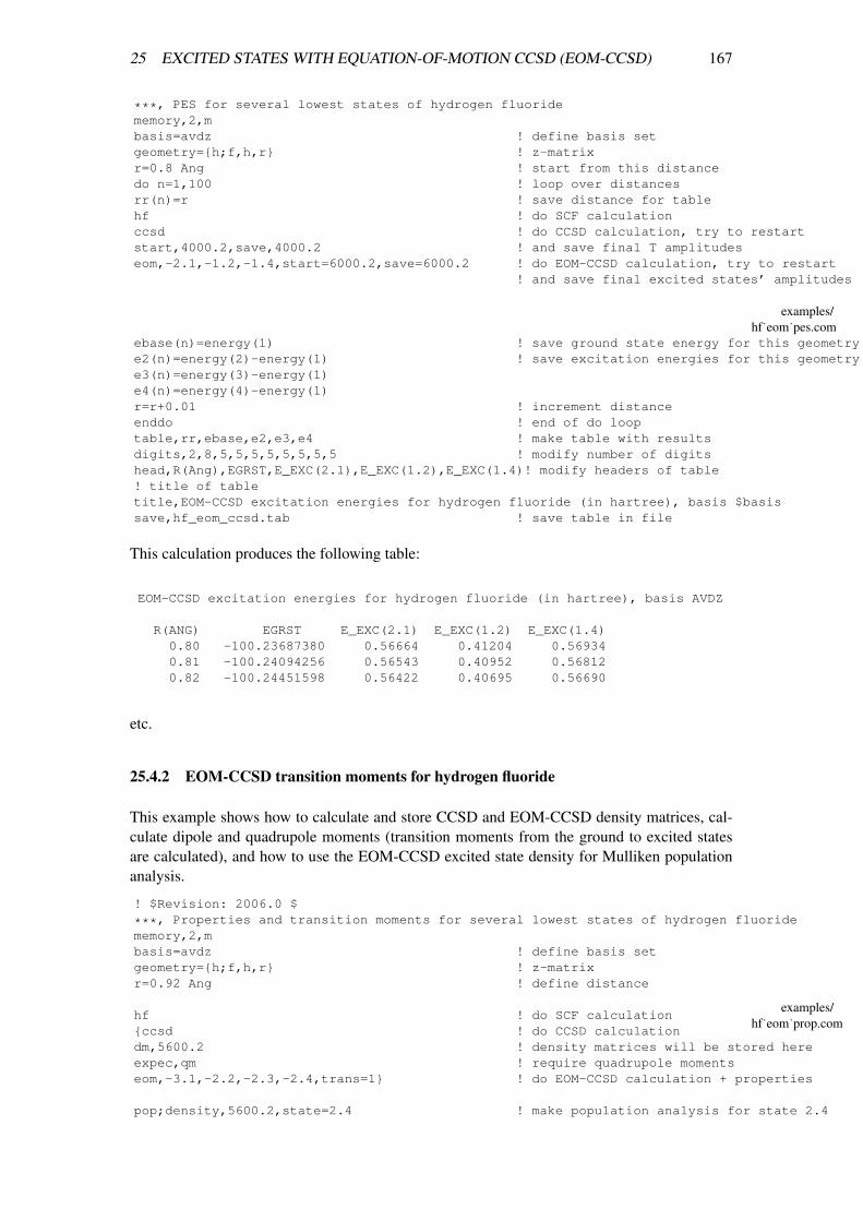
25 EXCITED STATES WITH EQUATION-OF-MOTION CCSD (EOM-CCSD) 167
***, PES for several lowest states of hydrogen fluoridememory,2,mbasis=avdz ! define basis setgeometry={h;f,h,r} ! z-matrixr=0.8 Ang ! start from this distancedo n=1,100 ! loop over distancesrr(n)=r ! save distance for tablehf ! do SCF calculationccsd ! do CCSD calculation, try to restartstart,4000.2,save,4000.2 ! and save final T amplitudeseom,-2.1,-1.2,-1.4,start=6000.2,save=6000.2 ! do EOM-CCSD calculation, try to restart
! and save final excited states’ amplitudes
ebase(n)=energy(1) ! save ground state energy for this geometrye2(n)=energy(2)-energy(1) ! save excitation energies for this geometrye3(n)=energy(3)-energy(1)e4(n)=energy(4)-energy(1)r=r+0.01 ! increment distanceenddo ! end of do looptable,rr,ebase,e2,e3,e4 ! make table with resultsdigits,2,8,5,5,5,5,5,5,5,5 ! modify number of digitshead,R(Ang),EGRST,E_EXC(2.1),E_EXC(1.2),E_EXC(1.4)! modify headers of table! title of tabletitle,EOM-CCSD excitation energies for hydrogen fluoride (in hartree), basis $basissave,hf_eom_ccsd.tab ! save table in file
examples/hf˙eom˙pes.com
This calculation produces the following table:
EOM-CCSD excitation energies for hydrogen fluoride (in hartree), basis AVDZ
R(ANG) EGRST E_EXC(2.1) E_EXC(1.2) E_EXC(1.4)0.80 -100.23687380 0.56664 0.41204 0.569340.81 -100.24094256 0.56543 0.40952 0.568120.82 -100.24451598 0.56422 0.40695 0.56690
etc.
25.4.2 EOM-CCSD transition moments for hydrogen fluoride
This example shows how to calculate and store CCSD and EOM-CCSD density matrices, cal-culate dipole and quadrupole moments (transition moments from the ground to excited statesare calculated), and how to use the EOM-CCSD excited state density for Mulliken populationanalysis.
! $Revision: 2006.0 $
***, Properties and transition moments for several lowest states of hydrogen fluoridememory,2,mbasis=avdz ! define basis setgeometry={h;f,h,r} ! z-matrixr=0.92 Ang ! define distance
hf ! do SCF calculation{ccsd ! do CCSD calculationdm,5600.2 ! density matrices will be stored hereexpec,qm ! require quadrupole momentseom,-3.1,-2.2,-2.3,-2.4,trans=1} ! do EOM-CCSD calculation + properties
pop;density,5600.2,state=2.4 ! make population analysis for state 2.4
examples/hf˙eom˙prop.com

25 EXCITED STATES WITH EQUATION-OF-MOTION CCSD (EOM-CCSD) 168
This calculation produces the following table:
--------------------------------------------------------------------------------Final Results for EOM-CCSD
(moments in a.u.)--------------------------------------------------------------------------------
State Exc. Energy (eV) X Y Z2.1 14.436
Right transition moment 0.00000000 0.00000000 0.65349466Left transition moment 0.00000000 0.00000000 0.68871635Dipole strength 0.45007246Oscillator strength 0.15917669Dipole moment 0.00000000 0.00000000 0.88758090
etc.
25.4.3 Calculate an EOM-CCSD state most similar to a given CIS state
This example shows how to force the convergence of the EOM-CCSD program to a state, whichresembles at most a given CIS state.
***, EOM-CCSD, vector following procedurememory,2,mbasis=avdz ! define basis setgeometry={h;f,h,r} ! z-matrixr=0.92 Ang ! define distancehf;save,2100.2 ! do SCF calculation, save orbitalscis,-4.4,exfile=6000.2 ! do CIS calculation, save amplitudesccsd;save,4000.2 ! do CCSD calculation, save amplitudeseom,-4.4,checkovlp=1,exfile=6000.2 ! do EOM-CCSD calculation,
! check overlap of singles with CIS vectors! stored in record given in exfile
eompar,inisingl=200,inidoubl=0 ! for first approximation take 200 single CSF! of approximate hamiltonian
ccsd;start,4000.2 ! do CCSD calculation, try to restarteom,2.4,follow=2,exfile=6000.2,checkovlp=1 ! do EOM-CCSD calculation for state closest
! to 2.4 CIS state, check overlap of singles! with CIS vectors stored in exfile
eompar,inisingl=200,inidoubl=0eomprint,loce=1 ! print overlaps of sample and EOM vectors in
! each iteration
examples/hf˙eom˙conv.com
In this example the CIS state 2.4 corresponds to the EOM-CCSD state 1.4!
25.5 Excited states with CIS
Excitation energies can also be calculated using the Configuration-Interaction Singles (CIS)method. This method cannot be expected to give accurate results, but can be used for quite largemolecules. The states to be computed are specified similarly as for EOM, e.g.
hfcis,-3.1,1.2,trans=1

26 OPEN-SHELL COUPLED CLUSTER THEORIES 169
26 OPEN-SHELL COUPLED CLUSTER THEORIES
Spin unrestricted (RHF-UCCSD) and partially spin restricted (RHF-RCCSD) open-shell coupledcluster theories as described in J. Chem. Phys. 99 (1993) 5219 (see also erratum , J. Chem.Phys., 112 (2000) 3106) are available in MOLPRO. In both cases a high-spin RHF referencewavefunction is used. No coupled cluster methods based on UHF orbitals are implemented inMOLPRO (the only correlation method in MOLPRO which uses UHF orbitals is UMP2). In thedescription that follows, the acronyms RCCSD and UCCSD are used, but the theories shouldnormally be referred to as RHF-RCCSD, RHF-UCCSD, in order to distinguish them from al-ternative ansatze based on spin-unrestricted orbitals. The program will accept either the full orabbreviated acronyms as input commands.
In the RCCSD theory certain restrictions among the amplitudes are introduced, such that thelinear part of the wavefunction becomes a spin eigenfunction (this is not the case in the UCCSDmethod, even if an RHF reference function is used). At present, the implementation of RCCSDis only preliminary, and no CPU time is saved by as compared to UCCSD. However, improvedalgorithms, as described in the above publication, are currently being implemented, and will beavailable in the near future.
The input is exactly the same as for closed-shell CCSD, except that RCCSD or UCCSD are usedas keywords. By default, the open-shell orbitals are the same as used in the RHF referencefunction, but this can be modified using OCC, CLOSED, and WF cards.
Perturbative triples corrections are computed as follows:
RCCSD(T), UCCSD(T) triples corrections are computed as defined by J. D. Watts, J. Gaussand R. J. Bartlett, J. Chem. Phys. 98 8718 (1993).
RCCSD[T], UCCSD[T] corrections are computed without contributions of single excita-tions (sometimes called CCSD+T(CCSD)) .
RCCSD-T, UCCSD-T triples corrections are computed as defined by M. J. O. Deegan andP. J. Knowles, Chem. Phys. Letters 227 (1994) 321.
In fact, all three contributions are always computed and printed. The following variables areused to store the results (here CCSD stands for either UCCSD or RCCSD):
ENERGY total energy for method specified in the input.
ENERGC total CCSD energy without triples.
ENERGT(1) total CCSD(T) energy.
ENERGT(2) total CCSD[T] energy.
ENERGT(3) total CCSD-T energy.
It should be noted that in open-shell cases the triples energy slightly depends on the treatment ofcore orbitals. In MOLPRO pseudo-canonical alpha and beta spin orbitals ( http://dx.doi.org/10.1016/S0009-2614(91)85118-G ) are generated by block-diagonalizing the corresponding Fock matrices in thespace of valence orbitals, leaving frozen core orbitals untouched. Some other programs includethe frozen core orbitals in the canonicalization and transformation. Because of core-valencemixing this leads to slightly different energies. Neither of the two methods can be regarded asbetter or more justified — it is just a matter of definition. However, the method in MOLPRO ismore efficient since the subsequent integral transformation involves only valence orbitals andno core orbitals.

27 THE MRCC PROGRAM OF M. KALLAY (MRCC) 170
27 The MRCC program of M. Kallay (MRCC)
An interface exists to use the MRCC program of M. Kallay and J. Gauss within Molpro.The license and source code of the MRCC program must be obtained from Mihaly Kallay<[email protected]>. Currently, only single reference methods with RHF referencefunctions are supported. Perturbative methods and CCn methods are only available for closed-shell. Furthermore, only serial execution is supported under MOLPRO, i.e. the mpp versioncannot be used.
27.1 Installing MRCC
A file mrcc.tar.gz will be provided by by M. Kallay. This file should be copied into di-rectory MRCC under the main MOLPRO directory. In this directory, a Makefile exists, andtyping ”make” will compile and install the MRCC program. The executables will be copied intothe MOLPRO bin directory and are automatically called by MOLPRO. Orbitals and other inputinformation are communicated via external files, transparent to the user. Once the program isinstalled, please run ”make mrcctest” in testjobs directory.
27.2 Running MRCC
The MRCC program is invoked by the command
MRCC,optionsdirectives
The available options summarized in Table 9. For a detailed description please refer to theMRCC manual of M. Kallay (file ”manual” the mrcc directory)
In MOLPRO the method to be used can be given as a string (option METHOD=string). The avail-able methods and the corresponding MRCC input parameters (see MRCC manual) as specifiedin Table 10.
Directives are usually not necessary, but the CORE, OCC, ORBITAL, MAXIT, directives workas in the MOLPRO CCSD program. In addition, the number of states can be given on a STATEdirective and this has the same meaning as the EOM NSTATES option.

27 THE MRCC PROGRAM OF M. KALLAY (MRCC) 171
Table 9: Options for MRCCOption Alias Default valuea MeaningMETHOD CALC CC(n) Computational method. See Table 10.EXCITATION LEVEL -1 Excitation level in cluster operatorRESTART CC RESTART 0 Restart option. If 1, restart with previous amplitudes.DIRECTORY DIR ’ ’ Subdirectory in which MRCC runs
(necessary for restart jobs)EOM NSING NSING -1 Number of excited singlet states in closed-shell caseEOM NTRIP NTRIP 0 Number of excited triplet states in closed-shell caseEOM NSTATES NDOUB -1 Number of states in open shell case.SYMM SYMMETRY -1 Symmetry of excited statesDENSITY IDENS 0 Parameter for density calculationHF 1 0 for UHF or ROHF, 1 for closed-shellNACTO 0 Number of active occupied orbitalsNACTV 0 Number of active virtual orbitalsSACC 0 Spin-adapted coupled clusterDBOC 0 Diagonal BO correctionMEMORY -1 MemoryTOL ENERGY -1.0 Energy convergence thresholdFREQ 0.0 Frequency for dynamic polarizabilitiesFILE fort Name for MRCC fortran filesCONVER ICONV 0 See mrcc manualCS 1 See mrcc manualDIAG 0 See mrcc manualMAXEX 0 See mrcc manualSPATIAL 1 See mrcc manuala) -1 means default value taken from MOLPRO

27 THE MRCC PROGRAM OF M. KALLAY (MRCC) 172
Table 10: Methods available in the MRCC programMRCC parameters
Key METHOD LEVEL NotesCI(n) configuration interaction methodsCISD 0 2CISDT 0 3CISDTQ 0 4CI(N) 0 N Specify excitation level N using LEVEL
CC(N) coupled cluster methodsCCSD 1 2CCSDT 1 3CCSDTQ 1 4CC(N) 1 N Specify excitation level N using LEVEL
CC(N-1)[N] coupled cluster methodsCCSD[T] 2 3CCSDT[Q] 2 4CC(N-1)[N] 2 N Specify excitation level N using LEVEL
CC(N-1)(N) coupled cluster methods. Also computes [n] correctionsCCSD(T) 3 3CCSDT(Q) 3 4CC(N-1)(N) 3 N Specify excitation level N using LEVEL
CC(n-1)(n) L methods (also computes (n) and [n] corrections)CCSD(T) L 4 3CCSDT(Q) L 4 4CC(N-1)(N) L 4 N Specify excitation level N using LEVEL
CC(n)-1a methodsCCSDT-1A 5 3CCSDTQ-1A 5 4CC(N)-1A 5 N Specify excitation level N using LEVEL
CC(n)-1b methodsCCSDT-1B 6 3CCSDTQ-1B 6 4CC(N)-1B 6 N Specify excitation level N using LEVEL
CCn methods (only for ground states)CC3 7 3CC4 7 4CCN 7 N Specify excitation level N using LEVEL
CC(n)-3 methodsCCSDT-3 8 3CCSDTQ-3 8 4CC(N)-3 8 N Specify excitation level N using LEVEL

27 THE MRCC PROGRAM OF M. KALLAY (MRCC) 173
Examples: Closed-shell ground-state calculations for H2O:
***,mrcc calculations for h2omemory,8,mgthresh,energy=1.d-8
geometry={o;h1,o,r;h2,o,r,h1,theta}theta=104r=1 angbasis=vdz
hfmrcc,method=cc3; !CC3 calculationmethod(1)=programe(1)=energy !the final energy is returned in variable energy
ccsd(t) !CCSD(T) calculation using Molpromethod(2)=’CCSD(T) (MOLPRO)’e(2)=energy
mrcc,method=ccsd(t) !CCSD(T) calculation using MRCCmethod(3)=’CCSD(T) (MRCC)’e(3)=energy
mrcc,method=ccsdt,dir=mrccdir !CCSDT calculation, run in directory mrccdirmethod(4)=programe(4)=energy
mrcc,method=ccsdt(q),restart=1,dir=mrccdir !CCSDT(Q) calculation!restart with previous amplitudes
method(5)=programe(5)=energy
mrcc,method=CC(n),excitation=4,restart=1,dir=mrccdir !CCSDTQ calculationmethod(6)=programe(6)=energy
table,method,e
examples/h2o˙mrcc.com
This yields
METHOD ECC3 -76.23912734CCSD(T) (MOLPRO) -76.23905150CCSD(T) (MRCC) -76.23905150CCSDT -76.23922746CCSDT(Q) -76.23976632CCSDTQ -76.23973043
Excitation energies for H2O:

27 THE MRCC PROGRAM OF M. KALLAY (MRCC) 174
***,h2o excitation energiesmemory,8,mgthresh,energy=1.d-8geometry={o;h1,o,r;h2,o,r,h1,theta}theta=104r=1 angbasis=vdzhf
ii=0s=2 !number of states in each symmetrydo sym=1,4 !loop over irrepsccsd;eom,-(s+0.1*sym);$p=molpro;save_energymrcc,method=ccsd, symm=sym,nstates=2;$p=mrcc;save_energymrcc,method=ccsdt,symm=sym,nstates=2;$p=mrcc;save_energys=1enddo
{table,method,prog,states,e,excsort,3}
save_energy={ !procedure to save results in variables!nogprint,variablee1=energy(1)do i=1,#energyii=ii+1e(ii)=energy(i)method(ii)=programprog(ii)=pstates(ii)=i+0.1*symexc(ii)=(e(ii)-e1)*toevend do}
examples/h2o˙mrcc˙eom.com
This yields
METHOD PROG STATES E EXCCCSD MOLPRO 1.1 -76.23580212 0.000CCSD MRCC 1.1 -76.23580212 0.000CCSDT MRCC 1.1 -76.23922746 0.000CCSD MOLPRO 1.2 -76.23580212 0.000CCSD MRCC 1.2 -76.23580212 0.000CCSDT MRCC 1.2 -76.23922746 0.000CCSD MOLPRO 1.3 -76.23580212 0.000CCSD MRCC 1.3 -76.23580212 0.000CCSDT MRCC 1.3 -76.23922746 0.000CCSD MOLPRO 1.4 -76.23580212 0.000CCSD MRCC 1.4 -76.23580212 0.000CCSDT MRCC 1.4 -76.23922746 0.000CCSD MOLPRO 2.1 -75.85033256 10.489CCSD MRCC 2.1 -75.85033257 10.489CCSDT MRCC 2.1 -75.85316687 10.505CCSD MOLPRO 2.2 -75.95093334 7.752CCSD MRCC 2.2 -75.95093335 7.752CCSDT MRCC 2.2 -75.95299013 7.789CCSD MOLPRO 2.3 -75.77630664 12.504CCSD MRCC 2.3 -75.77630665 12.504CCSDT MRCC 2.3 -75.77972816 12.504CCSD MOLPRO 2.4 -75.87776149 9.743CCSD MRCC 2.4 -75.87776150 9.743CCSDT MRCC 2.4 -75.88051189 9.761

27 THE MRCC PROGRAM OF M. KALLAY (MRCC) 175
Open-shell ground-state calculations for O2:
***,O2 testsmemory,8,mgthresh,energy=1.d-8
geometry={o1;o2,o1,r1}r1=2.2set,state=1,symmetry=4,spin=2 ! Triplet sigma- statebasis=vdz
rhfuccsd(t)method(1)=’UCCSD(T) MOLPRO’e(1)=energy
rccsd(t)method(2)=’RCCSD(T) MOLPRO’e(2)=energy
mrcc,method=ccsdt,dir=mrccdirmethod(3)=’CCSDT MRCC’e(3)=energy
mrcc,method=ccsdtq,restart=1,dir=mrccdirmethod(4)=’CCSDT MRCC’e(4)=energy
table,method,e
examples/o2˙mrcc.com
This yields
METHOD EUCCSD(T) MOLPRO -149.9815472RCCSD(T) MOLPRO -149.9812566CCSDT MRCC -149.9816705CCSDT MRCC -149.9832255

28 LOCAL CORRELATION TREATMENTS 176
28 LOCAL CORRELATION TREATMENTS
28.1 Introduction
The local correlation program of MOLPRO can currently perform closed-shell LMP2, LMP3,LMP4(SDTQ), LCISD, LQCISD(T), and LCCSD(T) calculations. For large molecules, allmethods scale linearly with molecular size, provided very distant pairs are neglected, and theintegral-direct algorithms are used.
Much higher efficiency is achieved by using density fitting (DF) approximations to computethe integrals. Density fitting is available for all local methods up to LCCSD(T), as well as foranalytical LMP2 gradients. Only iterative triples methods like LCCSDT-1b can currently not bedone with density fitting.
The errors introduced by DF are negligible, and the use of the DF methods is highly recom-mended. Linear scaling can be obtained in DF-LMP2 using the LOCFIT option (see Ref. 11);in DF-LCCSD(T), the most important parts also scale linearly, but some transformation stepsscale quadratically.
Energy gradients are available for LMP2, DF-LMP2, DF-SCS-LMP2, and LQCISD (in the lattercase only for LOCAL=1, i.e. the local calculation is simulated using the canonical program, andsavings only result from the reduced number of pairs).
Local explicitly correlated methods (DF-LMP2-R12 and DF-LMP2-F12 are described in section29.
Before using these methods, it is strongly recommended to read the literature in order to under-stand the basic concepts and approximations. A recent review [1] and Ref. [2] may be suitablefor an introduction.
References:
Review:[1] H.-J. Werner and K. Pfluger, On the selection of domains and orbital pairs in local correla-tion treatments, Ann. Rev. Comp. Chem., in press. (preprint available under http://www.theochem.uni-stuttgart.de/ werner/local/preprints/)
General local Coupled Cluster:[2] C. Hampel and H.-J. Werner, Local Treatment of electron correlation in coupled cluster(CCSD) theory, J. Chem. Phys. 104, 6286 (1996).[3] M. Schutz and H.-J. Werner, Local perturbative triples correction (T) with linear cost scal-ing, Chem. Phys. Letters 318, 370 (2000).[4] M. Schutz, Low-order scaling local electron correlation methods. III. Linear scaling localperturbative triples correction (T), J. Chem. Phys. 113, 9986 (2000).[5] M. Schutz and H.-J. Werner, Low-order scaling local electron correlation methods. IV. Lin-ear scaling local coupled-cluster (LCCSD), J. Chem. Phys. 114, 661 (2001).[6] M. Schutz, Low-order scaling local electron correlation methods. V. Connected Triples be-yond (T): Linear scaling local CCSDT-1b, J. Chem. Phys. 116, 8772 (2002).[7] M. Schutz, A new, fast, semi-direct implementation of Linear Scaling Local Coupled ClusterTheory, Phys. Chem. Chem. Phys. 4, 3941 (2002).
Multipole treatment of distant pairs:[8] G. Hetzer, P. Pulay, H.-J. Werner, Multipole approximation of distant pair energies in localMP2 calculations, Chem. Phys. Lett. 290, 143 (1998).
Linear scaling local MP2:[9] M. Schutz, G. Hetzer and H.-J. Werner, Low-order scaling local electron correlation meth-ods. I. Linear scaling local MP2, J. Chem. Phys. 111, 5691 (1999).

28 LOCAL CORRELATION TREATMENTS 177
[10] G. Hetzer, M. Schutz, H. Stoll, and H.-J. Werner, Low-order scaling local electron corre-lation methods II: Splitting the Coulomb operator in linear scaling local MP2, J. Chem. Phys.113, 9443 (2000).
Density fitted local methods:[11] H.-J. Werner, F. R. Manby, and P. J. Knowles, Fast linear scaling second-order Møller-Plesset perturbation theory (MP2) using local and density fitting approximations, J. Chem.Phys. 118, 8149 (2003). [12] M. Schutz and F.R. Manby, Linear scaling local coupled clustertheory with density fitting. Part I: 4- external integrals, Phys. Chem. Chem. Phys. 5, 3349(2003).[13] Polly, H.-J. Werner, F. R. Manby, and Peter J. Knowles, Fast Hartree-Fock theory usinglocal density fitting approximations, Mol. Phys. 102, 2311 (2004).[14] H.-J. Werner and M. Schutz, Low-order scaling coupled cluster methods (LCCSD(T)) withlocal density fitting approximations, in preparation.
LMP2 Gradients and geometry optimization:[15] A. El Azhary, G. Rauhut, P. Pulay and H.-J. Werner, Analytical energy gradients for localsecond-order Møller-Plesset perturbation theory, J. Chem. Phys. 108, 5185 (1998).[16] G. Rauhut and H.-J. Werner, Analytical Energy Gradients for Local Coupled-Cluster Meth-ods, Phys. Chem. Chem. Phys. 3, 4853 (2001).[17] M. Schutz, H.-J. Werner, R. Lindh and F.R. Manby, Analytical energy gradients for localsecond-order Møller-Plesset perturbation theory using density fitting approximations, J. Chem.Phys. 121, 737 (2004).
LMP2 vibrational frequencies:[18] G. Rauhut, A. El Azhary, F. Eckert, U. Schumann and H.-J. Werner, Impact of Local Ap-proximations on MP2 Vibrational Frequencies, Spectrochimica Acta 55, 651 (1999).[19] G. Rauhut and H.-J. Werner The vibrational spectra of furoxan and dichlorofuroxan: acomparative theoretical study using density functional theory and Local Electron CorrelationMethods, Phys. Chem. Chem. Phys. 5, 2001 (2003).[20] T. Hrenar, G. Rauhut and H.-J. Werner, Impact of local and density fitting approximationson harmonic vibrational frequencies, J. Phys. Chem. A., 110, 2060 (2006).
Intermolecular interactions and the BSSE problem:[21] M. Schutz, G. Rauhut and H.-J. Werner, Local Treatment of Electron Correlation in Molec-ular Clusters: Structures and Stabilities of (H2O)n, n = 2−4, J. Phys. Chem. 102, 5997 (1998).See also [2] and references therein.[22] N. Runeberg, M. Schutz and H.-J. Werner, The aurophilic attraction as interpreted by localcorrelation methods, J. Chem. Phys. 110, 7210 (1999).[23] L. Magnko, M. Schweizer, G. Rauhut, M. Schutz, H. Stoll, and H.-J. Werner, A Comparisonof the metallophilic attraction in (X-M-PH3)2 (M=Cu, Ag, Au; X=H, Cl), Phys. Chem. Chem.Phys. 4, 1006 (2002).
28.2 Getting started
The local correlation treatment is switched on by preceding the command name by an L, i.e., byusing the LMP2, LMP3, LMP4, LQCISD, LCCSD, or LCISD commands.
The LQCISD and LCCSD commands can be appended by a specification for the perturbativetreatment of triple excitations (e.g., LCCSD(T0)):
(T) Use the default triples method. Currently this is T0.
(T0) Non-iterative local triples. This is the fastest triples option. It is usually sufficientlyaccurate and recommended to be used in most cases.

28 LOCAL CORRELATION TREATMENTS 178
(T1) T0 plus one perturbative update of the triples amplitudes. If the accuracy of T0 isinsufficient (very rarely the case!), this can be used to improve the accuracy. Thecomputational cost is at least twice as large as for T0. In contrast to T0, the triplesamplitudes must be stored on disk, which can be a bottleneck in calculations forlarge molecules. Also the memory requirements are substantially larger than forT0.
(T1C) As T1, but a caching algorithm is used which avoids the simultaneous storage of alltriples amplitudes on disk (as is the case for (T1) or (TF)). Hence, T1C requiresless disk space but more CPU-time than T1. The more disk space is made availablefor the caching algorithm (using the T1DISK option on the local card, see below),the less CPU time is used.
(TF) Full iterative triples calculation. With full domains and without weak pair approx-imations this gives the same result as a canonical (T) calculation. Typically, 3-5iterations are needed, and therefore the computational effort is 2-3 times largerthan for (T1). The disk and memory requirements are the same as for T1. The T0energy is also computed and printed. TFULL and FULL are aliases for TF.
(TA) As TF, but the T1 energy is also computed. Since the first iteration is different forT1, the convergence of the triples iterations is slightly different with TF and TA(TF being somewhat faster in most cases). TALL and ALL are aliases for TA.
Density fitting can be invoked by prepending the command name by DF-, e.g. DF-LMP2,DF-LCCSD(T0) etc. In density fitting calculations an additional auxiliary basis set is needed.Details about choosing such basis sets and other options for density fitting are described insections 28.10 and 11.
The general input for local coupled LMP2 or coupled cluster calculations is:
LMP2,options Local MP2 calculation
LCCSD,options Local CCSD calculation
LCCSD(T0),options Local CCSD(T0) calculation
The same options as on the command line can also be given on subsequent LOCAL and MULTPdirectives. Instead of using the MULTP directive, the MULTP option on the command line canalso be used.
In the following, we will first give a summary of all options and directives. These will bedescribed in more detail in the subsequent sections. For new users it is recommended to readsection 28.9 at the end of this chapter before starting calculations.
28.3 Summary of options
Many options can be specified on the command line. For all options appropriate default valuesare set, and so these options must usually be modified only for special purposes. For convenienceand historical reasons, alias names are available for various options, which often correspond tothe variable name used in the program. Table 11 summarizes the options, aliases and defaultvalues. In the following, the parameters will be described in more detail.

28 LOCAL CORRELATION TREATMENTS 179
Table 11: Summary of local (multp) options and their default valuesParameter Alias Default value Meaning
General Parameters:LOCAL 4 determines which program to use.MULTP 0 turns on multipole approximations for distant pairs.SAVEDOM SAVE 0 specifies record for saving domain info.RESTDOM START 0 specifies record for reading domain info.PIPEK LOCORB 0 activates or deactivates PM localization.CANONICAL 0 allows to use canonical virtual orbitals (for testing).PMDEL CPLDEL 0 discards contributions of diffuse functions in PM localization.SAVORB SAVLOC 0 specifies record for saving local orbitals.DOMONLY 0 if 1, only domains are made.
if 2, only orbital domains are made.
Parameters to define domains:THRBP DOMSEL 0.98 Boughton-Pulay selection criterion for orbital domains.CHGMIN 0.01 determines the minimum allowed atomic charge in domains.CHGMINH 0.03 as CHGMIN, but used for H-atoms (default 0.03).CHGMAX 0.40 If the atomic charge is larger than this value,
the atom is always included in the domain.MAXANG MAXL 99 angular momentum restriction for BP domain selectionMAXBP 0 determines how atoms are ranked in BP procedure.MULLIKEN LOCMUL 0 determines the method to determine atomic charges.MERGEDOM 0 merges overlapping domains.DELCOR IDLCOR 2 delete projected core AOs up to certain shell.DELBAS IBASO 0 determines how to remove redundancies.
Distance criteria for domain extensions:REXT 0 criterion for all pair domains.REXTS 0 criterion for strong pair domains.REXTC 0 criterion for strong and close pair domains.REXTW 0 criterion for strong, close, and weak pair domains.
Connectivity criteria for domain extensions:IEXT 0 criterion for all pair domains.IEXTS 0 criterion for strong pair domains.IEXTC 0 criterion for strong and close pair domains.IEXTW 0 criterion for strong, close, and weak pair domains.
Parameters to select pair classes:USE DIST 1 determines if distance of connectivity criteria are used.RCLOSE CLOSEP 1 distance criterion for selection of weak pairs.RWEAK WEAKP 3 distance criterion for selection of weak pairs.RDIST DISTP 8 distance criterion for selection of distant pairs.RVDIST VERYD 15 distance criterion for selection of very distant pairs.ICLOSE 1 connectivity criterion for selection of weak pairs.IWEAK 2 connectivity criterion for selection of weak pairs.IDIST 5 connectivity criterion for selection of distant pairs.IVDIST 8 connectivity criterion for selection of very distant pairs.CHGMIN PAIRS CHGMINP 0.20 determines minimum charge of atoms used for pair
classification.KEEPCL 0 determines if close pairs are included in LCCSD.

28 LOCAL CORRELATION TREATMENTS 180
Parameter Alias Default value MeaningParameter for multipole treatment of exchange operators:DSTMLT 3 multipole expansion level for distant pairs
Parameters for energy partitioning:IEPART 0 If nonzero: do energy partitioning.EPART 3.0 cutoff parameter for determining individual monomers.
Parameters for redundancy check using DELBAS=1 (not recommended)TYPECHECK TYPECHK 1 activates basis function type restrictions.DELSHL IDLSHL 1 determines if whole shells are to be deleted.DELEIG IDLEIG 1 determines how to select redundant functions.DELCMIN CDELMIN 0.1 parameter for use with DELEIG=1
Parameters for choosing operator domains in LCCSDOPDOM IOPDOM 5 determines how operator domains are determined for LCCSDRMAXJ 8 distance criterion for J-operator list.RMAXK 8 distance criterion for K-operator list.RMAXL 15 distance criterion for L-operator list.RMAX3X 5 distance criterion for 3-ext integral list.RDOMJ 0 distance criterion for K-operator domains.RDOMK 8 distance criterion for J-operator domains.IMAXJ 5 connectivity criterion for J-operator list.IMAXK 5 connectivity criterion for K-operator list.IMAXL 8 connectivity criterion for L-operator list.IMAX3X 3 connectivity criterion for 3-ext integral list.IDOMJ 0 connectivity criterion for K-operator domains.IDOMK 5 connectivity criterion for J-operator domains.
Miscellaneous options:SKIPDIST SKIPD 3 determines at which stage weak and distant pairs are eliminatedASYDOM JITERM 0 parameter for use of asymmetric domainsLOCSING LOCSNG 0 determines virtual space used for singlesPIPEKAO LOCAO 0 activates AO localization criterionNONORM 2 determines whether projected functions are normalizedLMP2ALGO MP2ALGO 3 if nonzero, use low-order scaling method in LMP22 iterationsOLDDEF 0 allows to revert to older defaultsT1DISK 10 maximum disk space (in GByte) for T1 caching algorithm
Thresholds:THRBP 0.98 Threshold Boughton-Pulay method.THRPIP 1.d-12 Threshold for Pipek-Mezey localization.THRORB 1.d-6 Threshold for eliminating projected orbitals with small norm.THRLOC 1.d-6 Threshold for eliminating redundant projected orbitals.THRCOR 1.d-1 Threshold for eliminating projected core orbitals.THRMP2 1.d-8 Threshold for neglecting small fock matrix elements in the
LMP2 iteration.

28 LOCAL CORRELATION TREATMENTS 181
28.4 Summary of directives
The same standard directives as in the canonical programs, e.g., OCC, CLOSED, CORE, WF,ORBITAL are also valid in the local methods. In addition, there are some directives which onlyapply to local calculations:
LOCAL Invokes local methods and allows to specify the same options as onthe command line.
MULTP As LOCAL, but multipole approximations are used for distant pairs.
DOMAIN Define domains manually (not recommended).
MERGEDOM Allows to merge domains
REGION Allows to select regions of a molecule to be treated at a certain levelof theory.
ENEPART Analysis of pair energies.
SAVE Save domains and LCCSD amplitudes.
START Restart with domains and LCCSD amplitudes from a previous calcu-lation.
28.5 General Options
LOCAL=local Determines which method is used:LOCAL=0: Conventional (non-local) calculation.LOCAL=1: Local method is simulated using canonical MOs. The lo-cal basis is used only at an intermediate stage to update the amplitudesin each iteration (only for testing).LOCAL=2: Calculation is done in local basis, but without using lo-cal blocking (i.e. full matrices are used). This is the most expensivemethod and only for testing.LOCAL=3: Fully local calculation (obsolete).LOCAL=4: Fully local calculation (default). This is the fastest methodfor large molecules with many weak pairs and requires minimummemory.
PIPEK=option If this option is given and option> 0, the orbitals are localized usingthe Pipek-Mezey technique. If this option is not given or option=0(default), the orbitals are localized unless localized orbitals are foundin the orbital record (cf. ORBITAL directive and LOCALI command).In the latter case, the most recent localized orbitals are used. Settingoption=-1 switches the localization off. If option> 1 the localizedorbitals are printed. Note: Boys localization can only be performedusing the LOCALI command. The program will use the Boys orbitalsif they are found in the orbital record and the PIPEK option is absentor option≤ 0.
SAVORB=record Allows the localized and projected orbitals to be saved in record=name.ifilfor later use (e.g. plotting). The two orbital sets are stored in the samedump record and can be restored at later stages usingORBITAL,record,[TYPE=]LOCAL orORBITAL,record,[TYPE=]PROJECTED, respectively.

28 LOCAL CORRELATION TREATMENTS 182
DOMONLY=value If value> 0 only domains are made, but no energy is computed. Thiscan be used to check and save the domains for later use.
DSTMLT=level Determines the expansion level of the multipole expansion of distantpairs (e.g. 1 means dipole approximation, 2 quadrupole approxima-tion and so on). The default for MULTP is 3.
INTERACT Automatically determine individual molecules in a calculation and setappropriate pair lists for computing interaction energies. See section28.9.8 for more details.
Parameters for energy partitioning:
IEPART=value enables/disables energy partitioning.iepart=0: Energy partitioning is disabled.iepart=1: Energy partitioning is enabled.iepart=2: Energy partitioning is enabled. Additionally, a list of allpair energies and their components is printed.
EPART=cutoff Cutoff parameter to determine individual monomers in a cluster (i.e.centre groups). Should be somewhat larger than the largest intramolec-ular bond length (given in a.u.).
Miscellaneous options:
SKIPDIST=skipdist Test-parameter. Its value should only affect the efficiency but not in-fluence the results.skipdist=-1: Weak and distant pairs are set to zero after MP2 but arenot eliminated from the pair list and not skipped in any loop.skipdist=0: No pairs are deleted from pair list, but weak and distantpairs are skipped in the loops were appropriate.skipdist=1: Very distant pairs are neglected from the beginning. Dis-tant pairs are eliminated after MP2.skipdist=2: As skipdist=1, but also weak pairs are eliminated afterMP2.skipdist=3: As skipdist=2, but distant pairs are eliminated from theoperator list in case of LMP2 with multipole approximations for dis-tant pairs. This is the default.
ASYDOM=jiterm Experimental test parameter. Enables the use of asymmetric domainsfor distant pairs. The asymmetric domain approximation supplementsthe multipole approximation for distant pairs, as it suppresses thetreatment of configurations for which no integrals can be computedby multipole expansion. This leads to computational savings and im-proved numerical stability.jiterm=0: Disable asymmetric domains.jiterm=-1: Enable asymmetric domains (default).jiterm=-2: Enable a variation of the asymmetric domain formalism:Exchange operators will initially be projected to the asymmetric do-main instead of simply packed.
LOCSING=locsing If locsing.ne.0, the single excitations use the full space, i.e., they arenot treated locally. This is only works for LOCAL=1.
MAXANG=lmax The purpose of this experimental option is to reduce the basis setsensitivity of the Boughton-Pulay (BP) method for domain selection.Only basis functions with angular momentum up to lmax-1 are in-cluded when computing the overlap of the approximate and exact or-

28 LOCAL CORRELATION TREATMENTS 183
bitals. For example, MAXANG=2 means to omit all contributions ofd, f and higher angular momentum functions. To obtain reasonabledomains, the value of THRBP must often be reduced (to 0.97 or so).This option should only be used with care!
PIPEKAO=option If option≥ 0, the orbitals are localized my maximizing the coefficientsof basis functions of a given type at a given atom. Normally, this isonly useful to uniquely define degenerate orbitals in atoms. For in-stance, when this option is used to localize the orbitals for a dimerlike (Ar)2 at a very long distance, clean s, px, py, and pz atomic or-bitals will be obtained. It is not recommended to use this option formolecular calculations!
NONORM=value Determines if projected functions are normalized (not recommended).value=-1: projected orbitals are normalized before redundancy check.value=0: projected orbitals are normalized after redundancy check(default).value=1: projected orbitals are normalized in redundancy check, af-terwards unnormalized.value=2: projected orbitals are never normalized (default in gradientcalculations).
LMP2ALGO=value If nonzero, use low-order scaling method in LMP2 iterations. Valuescan be 1, 2, or 3, and 3 is usually fastest if large basis sets are used.
OLDDEF=value For compatibility with older versions: if nonzero, revert to old de-faults. Options set before this may be overwritten.
Thresholds:
THRPIP=thresh Threshold for Pipek-Mezey localization. The localization is assumedto be converged if all 2×2 rotation angles are smaller then thresh. Thedefault is 1.d−12. It can also be modified globally using GTHRESH,LOCALI=thresh.
THRORB=thresh Threshold for eliminating functions from pair domains whose normis smaller then thresh after projecting out the occupied space. Thedefault is throrb=1.d-6.
THRLOC=thresh Threshold for eliminating redundant basis functions from pair do-mains. For each eigenvalue of Si j < thresh one function is deleted.The default is 1.d-6. The method used for deleting functions dependson the parameters IDLEIG and IBASO.
THRMP2=thresh Threshold for neglecting small fock matrix couplings in the LMP2iterations (default 1.d-8). Specifying a larger threshold speeds up theiterations but may lead to small errors in the energy. In the initialiterations, a larger threshold is chosen automatically. It is graduallyreduced to the specified final value during the iterations.
THRCOR=thresh Threshold for deleting projected core orbitals. The functions are onlydeleted if their norm is smaller than thresh (default 0.1)
The thresholds can also be specified on the THRESH directive.
28.6 Options for selection of domains
The following sections describe the most important options which affect the domains.

28 LOCAL CORRELATION TREATMENTS 184
28.6.1 Standard domains
Standard domains are always determined first. They are used to define strong, close, weak, anddistant pairs. More accurate results can be obtained with extended domains, as described insection 28.6.2.
THRBP=value Threshold for selecting the atoms contributing to orbital domains us-ing the method of Boughton and Pulay (BP). As many atoms as neededto fulfill the BP criterion are included in a domain. The order in whichatoms are considered depends on the parameter MAXBP, see below.The default is THRBP=0.98. THRBP=1.0 includes all atoms intoeach orbital domain, i.e., leads to full domains. If no pairs are ne-glected, this should yield the canonical MP2 energy.
The criterion is somewhat basis dependent. See section 28.9.4 forrecommended values of this threshold.
CHGMIN=value determines the minimum allowed Mulliken (or Lowdin) charge foran atom (except H) in a domain, i.e., atoms with a smaller (absolute)charge are not included, even if the THRBP criterion is not fulfilled(default 0.01).
CHGMINH=value as CHGMIN, but used for H-atoms (default 0.03).
CHGMAX=value If the atomic charge is larger than this value, the atom is included,independent of any ranking.
MAXBP=maxbp If maxbp=1, the atoms are ranked according to their contribution tothe Boughton-Pulay overlap. If maxbp=0 (default), the atoms areranked according to atomic charges. In both cases atoms with chargesgreater than CHGMAX are always included, and atoms with the samecharges are added as groups.
MULLIKEN=option Determines the method to determine atomic charges. MULLIKEN=0(default): squares of diagonal elements of S
12 C are used (Lowdin
charges); MULLIKEN=1: Mulliken gross charges are used. The firstchoice is less basis set dependent and more reliable with diffuse basissets.
MERGEDOM=number If number is greater than zero, all orbital domains containing numberor more atoms in common are merged (number=1 is treated as num-ber=2, default 0). This is particularly useful for geometry optimiza-tions of conjugated or aromatic systems like, e.g., benzene. In the lat-ter case, MERGEDOM=1 causes the generation of full π-domains, i.e.,the domains for all three π-orbitals comprise all carbon basis func-tions. Note that the merged domains are generated after the aboveprint of orbital domains, and information about merged domains isprinted separately. See section 28.9.7 for further discussion of geom-etry optimizations.
There are some other options which should normally not be modified:
DELBAS=ibaso This parameter determines the method for eliminating redundantfunctions of pair domains.ibaso=0: The space of normalized eigenvectors of Si j, whichcorrespond to small eigenvalues, is eliminated (default). Any other

28 LOCAL CORRELATION TREATMENTS 185
value is not recommended and not further documented.
DELCOR=nshell Activates elimination of basis functions corresponding to core or-bitals. If nshell=1, only 1s-functions are eliminated from projectedspace. If nshell=2 (default) 1s functions on first-row atoms, and 1s,2s, and 2p-functions are eliminated on second-row atoms. Nothingis eliminated on H or He atoms. If effective core potentials are used,nothing is deleted at the corresponding atom. Also, functions are onlydeleted if the norm of the projected function is below THRCOR (de-fault 0.1)
28.6.2 Extended domains
There are two alternative modes for domain extensions: either distance criteria REXT, REXTS,REXTC, or REXTW can be used. These are in Bohr and refer to the minimum distance betweenany atom in a standard orbital domain [i j] and another atom. If an atom is found within thegiven distance, all PAOs at this atom are added to the domain [i j]. Alternatively, connectivitycriteria IEXT, IEXTS, IEXTC, or IEXTW can be used. These refer to the number of bondsbetween any atom contained in the standard domain [i j] and another atom. The advantage ofdistance criteria is that they select also atoms within the given radius which are not connectedto the present domain by bonds. On the other hand, the connectivity criteria are independent ofdifferent bond lengths, e.g., for first and second-row atoms. Only one of the two possibilitiescan be used, i.e., they are mutually exclusive.
REXT=value Distance criterion for extension of all pair domains.
REXTS=value Distance criterion for extension of strong pair domains.
REXTC=value Distance criterion for extension of strong and close pair domains.
REXTW=value Distance criterion for extension of strong, close, and weak pair do-mains.
IEXT=value Connectivity criterion for extension of all pair domains.
IEXTS=value Connectivity criterion for extension of strong pair domains.
IEXTC=value Connectivity criterion for extension of strong and close pair domains.
IEXTW=value Connectivity criterion for extension of strong, close, and weak pairdomains.
By default, domains are not extended, i.e., the default values of all parameters listed aboveare zero. Note that the pair classes are determined on the basis of the standard domains, andtherefore domain extensions have no effect on the pair lists.
Also note that the computational effort increases with the fourth power of the domain sizes andcan therefore increase quite dramatically when extending domains. This does not affect thelinear scaling behaviour in the asymptotic limit.
28.6.3 Manually Defining orbital domains (DOMAIN)
It is possible to define the domains “by hand”, using the DOMAIN directive:
DOMAIN,orbital,atom1, atom2 . . .

28 LOCAL CORRELATION TREATMENTS 186
where orbital has the form iorb.isym, e.g., 3.1 for the third orbital in symmetry 1, and atomiare the atomic labels as given in the Z-matrix geometry input, or, alternatively, the Z-matrixrow numbers. All basis functions centred at the given atoms are included into the domain. Forinstance
DOMAIN,3.1,C1,C2
defines a domain for a bicentric bond between the carbon atoms C1 and C2. The DOMAIN di-rective must be given after any OCC, CLOSED, or CORE directives. Note that the order of thelocalized orbitals depends on the localization procedure, and could even change as function ofgeometry, and therefore manual DOMAIN input should be used with great care. The domains ofall orbitals which are not explicitly defined using DOMAIN directive are determined automati-cally as usual.
28.7 Options for selection of pair classes
There are two alternative modes for defining the pair classes: either distance criteria RCLOSE,RWEAK, RDIST, RVDIST can be used. These are in Bohr and refer for a given orbital pair(i j) to the minimum distance R(i j) between any atom in the standard orbital domains [i] andany atom in the standard orbital domains [ j] . Alternatively, the connectivity criteria ICLOSE,IWEAK, IDIST, IVDIST can be used. These refer to the minimum number of bonds betweenany atom contained in the standard domain [i] and any atom contained in the standard domain [ j]The advantage of using connectivity criteria is the independence of the bond lengths, while theadvantage of distance criteria (default) is that they are also effective in non-bonding situations.Only one of the two possibilities can be used, i.e., they are mutually exclusive. The use ofdistance criteria is the default. Using connectivity criteria for pair selection requires to set theoption USE DIST=0.
USE DIST (default 1) If nonzero, use distance criteria, otherwise connectivitycriteria.
CHGMIN PAIRS Only atoms in the primary domains are considered for the pair classi-fication if the atomic Lowdin charge is larger than CHGMIN PAIRS(default value 0.2). This criterion was introduced in order to reducethe dependence of the pair selection on localization tails.
RCLOSE (default 1) Strong pairs are defined by 0 ≤ R(i j) < RCLOSE. Closepairs are defined by RCLOSE≤ R(i j) < RWEAK.
RWEAK (default 3) Weak pairs are defined by RWEAK≤ R(i j) < RDIST.
RDIST (default 8) Distant pairs are defined by RDIST≤ R(i j) < RVDIST.
RVDIST (default 15) Very distant pairs for which R(i j) ≥RVDIST are neglected.
ICLOSE (default 1) Strong pairs are separated by less that ICLOSE bonds.Close orbital pairs are separated by at least ICLOSE bonds but lessthan IWEAK bonds.
IWEAK (default 2) Weak orbital pairs are separated by at least IWEAK bondsbut less than IDIST bonds.
IDIST (default 5) Distant orbital pairs are separated by at least IDIST bondsbut less than IVDIST bonds.
IVDIST (default 8) Very distant orbital pairs (neglected) are separated by atleast IVDIST bonds.

28 LOCAL CORRELATION TREATMENTS 187
KEEPCL (default 0) If KEEPCL=1, the LMP2 amplitudes of close pairs areincluded in the computation of the strong pair LCCSD residuals. IfKEEPCL=2 all close pairs are fully included in the LCCSD (this doesnot affect the triples list). This option is not yet implemented as effi-ciently as it could, and can therefore lead to a significant increase ofthe CPU time.
Setting a distance criterion to zero means that all pairs up to the corresponding class are treatedas strong pairs. For instance, RCLOSE=0 means that strong and close pairs are fully includedin the LCCSD (in this case KEEPCL=1 has no effect). Note, however, that setting RCLOSE=0increases the length of the triples list.
28.8 Directives
28.8.1 The LOCAL directive
The LOCAL directive can be used to specify options for local calculations. If this directiveis inside the command block of a local calculation, the options are used only for the currentcalculation, and this is entirely equivalent as if they were specified on the command line. TheLOCAL directive can also be given outside a command block, and in this case the options areused for all subsequent local correlation calculations in the same input.
Example:
DF-LMP2,THRBP=0.985
is equivalent to
{DF-LMP2LOCAL,THRBP=0.985}
In the following example the LOCAL directive is global and acts on all subsequent local calcu-lations, i.e. both calculations will use THRBP=0.985
LOCAL,THRBP=0.985DF-LMP2 !local MP2 calculationOPTG !geometry optimization using the DF-LMP2 energyDF-LCCSD(T) !local coupled cluster at the optimized structure.
28.8.2 The MULTP directive
The MULTP directive turns on the multipole approximations for distant pairs, as described inRef. [8]. Further options can be given as described above for the LOCAL directive.
LOCAL,MULTP,options
is equivalent to
MULTP,options
The level of the multipole approximation can be chosen using option DSTMLT (default 3) ( 1means dipole approximation, 2 quadrupole approximation and so on).

28 LOCAL CORRELATION TREATMENTS 188
The multipole approximation reduces the computational cost of LMP2 calculations for verylarge molecules, but leads to some additional errors, see Ref. [8]. It is normally not recom-mended to be used in coupled-cluster calculations and should never be used for computing in-termolecular forces. It can also not be used in geometry optimizations or gradient calculations.
28.8.3 Saving the wavefunction (SAVE)
The wavefunction can be saved for later restart using
SAVE,record
where record has the usual form, e.g., 4000.2 means record 4000 on file 2. If this directive isgiven, the domain information as well as the amplitudes are saved (for MPn the amplitudes arenot saved). If just the domain information should be stored, the SAVE option on the LOCALdirective must be used (cf. section 28.3).
28.8.4 Restarting a calculation (START)
Local CCSD or QCISD calculations can be restarted using
START,record
The record given must have been saved in a previous local calculation using the SAVE directive(otherwise this directive is ignored). If the START directive is given, the domain informationas well as the amplitudes of the previous calculation are used for restart. It is possible, forinstance, to start a local CCSD calculation with the amplitudes previously saved for a localQCISD calculation (but of course it is not possible to use a record saved for a non-local CCSD orQCISD calculation). If it is intended only to use the domain information but not the amplitudesfor a restart, the START option on the command line or LOCAL directive must be used (cf.section 28.3).
28.8.5 Correlating subsets of electrons (REGION)
In large molecules, it may be sufficient to correlate only the electrons in the vicinity of anactive group, and to treat the rest of the molecule at the SCF level. This approach can evenbe extended, different correlation levels may be used for different sections of the system. TheREGION directive allows the specification of a subset of atoms:
REGION,METHOD=method,[DEFAULT=default method], [TYPE=INCLUSIVE|EXCLUSIVE],atom1, atom2 . . .
The orbitals located at these atoms will be treated at the level specified in method. The remainingorbitals will be treated as defined in default. If not given by the user, the latter option will be setto HF.
The orbital selection can be done in two ways. If type is set to INCLUSIVE, any orbital con-taining one of the atoms in its domain centre list will be included. If type is set to EXCLUSIVE,the program will only add orbitals whose domains are exclusively covered by the given atoms.Any local correlation treatment can be given as method, with the restriction that only MP2 andHF can be used as default method. Up to two REGION directives may be included in a singlecalculation, ordered according to the correlation level (method) specified for the region. Thehighest level region should be given last.

28 LOCAL CORRELATION TREATMENTS 189
It is advisable to check the region orbital list and the orbital domains printed by the program.The use of regions may significantly reduce the computation time, and, provided the activeatoms are sensibly chosen, may give still sufficiently accurate results for the active group, e.g.bond lengths and bond angles.
28.8.6 Domain Merging (MERGEDOM)
The restriction of the virtual space in local calculations may result in discontinuities for reactionpath calculations due to changes of the geometry dependent domains. This may be avoided bythe use of a MERGEDOM directive
MERGEDOM,[NEIGHBOUR=value],[CENTERS=[atom1, atom2. . . ]], [RECORD=. . . ],CHECK
This directive provides augmented domains, which can be saved (using option or directiveSAVE, see section 28.8.3) for later use in reaction paths or in single point calculations (in caseswhere the orbital domain description is unbalanced). The use of the neighbour option works inthe same way as the local option MERGEDOM, with value specifying the number of coincidentcentres. If the centres option is used, an atom list should be given (enclosed by square brackets).The domains of all orbitals located exclusively at these atoms will be merged, and the resultingmerged domains will be used for all these orbitals.
One may also give a record number from a previously saved local calculation. The domainlist contained in the record will be matched to the current one, and orbital domains augmented(merged) to include both sets. This domain definition should then be adequate for calculationson both points (and all those in between). This procedure can be repeated to include moregeometries. In this way domains can be defined that are appropriate for a whole range of ge-ometries (e.g. a reaction path), and if these domains are used in all calculations a strictly smoothpotential energy surface is obtained.
28.8.7 Energy partitioning for molecular cluster calculations (ENEPART)
The local character of occupied and virtual orbitals in the local correlation treatment also of-fers the appealing possibility to decompose the intermolecular interaction energy of molecularclusters into individual contributions of different excitation classes. This allows to distinguishbetween intramolecular-, dispersive-, and ionic components of the correlation contribution tothe interaction energy (cf. M. Schutz, G. Rauhut and H.J. Werner, J. Phys. Chem. 102, 5197(1998)). The energy partitioning algorithm is activated either by supplying the ENEPART direc-tive:
ENEPART,[epart],[iepart]
or by giving the parameters as options on the command line.
The epart parameter determines the cutoff distance for (intramolecular) bond lengths (in a.u.,default 3 a.u.) and is used to automatically determine the individual monomer subunits of thecluster. The iepart parameter enables the energy partitioning, if set to a value larger than zero(default 1). Additionally, if iepart is set to 2, a list of all intermolecular pair energies and theircomponents is printed.
The output section produced by the energy partitioning algorithm will look similar to the fol-lowing example:
energy partitioning enabled !centre groups formed for cutoff [au] = 3.001 :O1 H11 H12

28 LOCAL CORRELATION TREATMENTS 190
2 :O2 H21 H22energy partitioning relative to centre groups:intramolecular correlation: -.43752663exchange dispersion : .00000037dispersion energy : -.00022425ionic contributions : -.00007637
The centre groups correspond to the individual monomers determined for epart=3. In thepresent example, two water monomers were found. The correlation energy is partitioned intothe four components shown above. The exchange dispersion, dispersion and ionic componentsreflect directly the related intermolecular components of the complex, while the intramolecu-lar correlation contribution to the interaction energy has to be determined by a super-molecularcalculation, i.e. by subtracting the (two) corresponding monomer correlation energies from theintramolecular correlation component of the complex given in the output.
Alternatively, the following form can be used:
ENEPART,RMAX=[r1,r2,r3,. . .]
and the program will then print the energy contributions of all pairs in the ranges between thegiven distances (in bohr, enclosed by square brackets, e.g., enepart,rmax=[0,3,5,7,9,11]).A second list in which the contributions are given as a function of the number of bonds betweenthe pair domains will also be printed.
28.9 Doing it right
The local correlation methods in MOLPRO employ localized molecular orbitals (LMOs). Pipek-Mezey localization is recommended, but Boys localization is also possible. The virtual orbitalspace is spanned by non-orthogonal projected atomic orbitals (PAOs). The local character of thisbasis makes it possible to introduce two distinct approximations: first, excitations are restrictedto domains, which are subspaces of (PAOs) that are spatially close to the orbitals from whichthe electrons are being excited. Secondly, the orbital pairs are classified according to theirimportance (based on distance or connectivity criteria), and only strong pairs are treated atthe highest level (e.g. CCSD). The remaining weak and distant pairs are treated at the LMP2level, and very distant pairs are neglected. These approximations lead to linear scaling of thecomputational resources as a function of the molecular size.
Naturally, such approximation can introduce some errors, and therefore the user has to be morecareful than with standard black box methods. On the other hand, the low-order scaling makesit possible to treat much larger systems at high levels of theory than it was possible so far.
This section summarizes some important points to remember when performing local correlationcalculations.
28.9.1 Basis sets
For numerical reasons, it is useful to eliminate projected core orbitals, since these may havea very small norm. By default, projected core orbitals are eliminated if their norm is smallerthen 0.1 (this behaviour can be changed using the DELCOR and THRCOR options). For localcalculations we recommend the use of generally contracted basis sets, e.g., the correlation con-sistent cc-pVnZ sets of Dunning and coworkers. For these basis sets the core basis functions areuniquely defined, and will always be eliminated if the defaults for DELCOR and THRCOR areused.

28 LOCAL CORRELATION TREATMENTS 191
The correlation consistent basis sets are also recommended for all density fitting calculations,since optimized fitting basis sets are available for each basis.
28.9.2 Symmetry and Orientation
1. Turn off symmetry! Otherwise, you won’t get appropriately localized orbitals (local orbitalswill tend to be symmetry equivalent instead of symmetry adapted). Symmetry can be used onlyif all atoms are symmetry unique. This allows the local treatment of planar molecules in Cs
symmetry. But note that neither the multipole program nor the density fitting programs supportsymmetry at all, so choose always C1 symmetry for DF-calculations or with the MULTP option.
To turn off symmetry, specify NOSYM as the first line of your geometry input, e.g.
geometry={nosymO1H1,O1,rohH2,O1,roh,h1,hoh
}
Alternatively, add
SET,ZSYMEL=NOSYM
before the geometry block.
2. Use NOORIENT! We recommend to use the NOORIENT option in the geometry input, toavoid unintended rotations of the molecule when the geometry changes. This is particularly im-portant for geometry optimizations and for domain restarts in calculations of interaction energies(see section 28.9.8).
28.9.3 Localization
By default, Pipek-Mezey localization is used and performed automatically in the beginning of alocal correlation calculation. Thus
df-hf !Hartree-Fock with density fittingdf-lmp2 !LMP2 using the Pipek-Mezey LMOs
is equivalent to
df-hf !Hartree-Fock with density fittinglocali,pipek !Orbital localization using the Pipek-Mezey criteriondf-lmp2 !LMP2 using the Pipek-Mezey LMOs
Boys localization can be used as well, but in this case the localization must be done beforehand,e.g.
df-hf !Hartree-Fock with density fittinglocali,boys !Orbital localization using the Boys criteriondf-lmp2 !LMP2 using the Boys LMOs

28 LOCAL CORRELATION TREATMENTS 192
Poor localization is sometimes an intrinsic problem, in particular for strongly conjugated sys-tems or when diffuse basis sets are used. This is caused by localization tails due to the over-lapping diffuse functions. The problem is particularly frequent in calculations of systems withshort bonds, e.g., aromatic molecules. It can be avoided using directive
PIPEK,DELETE=n
with n = 1 or 2. This means that the contributions of the n most diffuse basis functions of eachangular momentum type are ignored in the localization. This often yields much better localizedorbitals when diffuse basis sets are used. For aug-cc-pVTZ, n = 2 has been found to work verywell, while for aug-cc-pVDZ n=1
In rare cases it might also happen that the localization procedure does not converge. It is thempossible to choose a second-order Newton-Raphson localization scheme, using the directive
PIPEK,METHOD=2,[DELETE=n]
28.9.4 Orbital domains
The orbital domains are determined automatically using the procedure of Boughton and Pulay, J.Comput. Chem., 14, 736 (1993) and J. Chem. Phys. 104, 6286 (1996). For higher accuracy thedomains can be extended, and in this way the canonical result can be systematically approached(cf. Ref. [1] and section 28.6.2). Details are described in section 28.6.
In most cases, the domain selection is uncritical for saturated molecules. Nevertheless, in partic-ular for delocalized systems, it is recommended always to check the orbital domains, which areprinted in the beginning of each local calculation. For such checking, the option DOMONLY=1can be used to stop the calculation after the domain generation. The orbital domains consist ofall basis functions for a subset of atoms. These atoms are selected so that the domain spans thecorresponding localized orbital with a preset accuracy (alterable with option THRBP). A typicaldomain output, here for water, looks like this:
Orbital domains
Orb. Atom Charge Crit.2.1 1 O1 1.17 0.00
3 H2 0.84 1.003.1 1 O1 2.02 1.004.1 1 O1 1.96 1.005.1 1 O1 1.17 0.00
2 H1 0.84 1.00
This tells you that the domains for orbitals 2.1 and 5.1 comprise the basis functions of theoxygen atom and and one hydrogen atom, while the domains for orbitals 3.1 and 4.1 consistof the basis function on oxygen only. The latter ones correspond to the oxygen lone pairs, theformer to the two OH bonds, and so this is exactly what one would expect. For each domain ofAOs, corresponding projected atomic orbitals (PAOs) are generated, which span subspaces ofthe virtual space and into which excitations are made. Options which affect the domain selectionare described in section 28.6. Improper domains can result from poorly localized orbitals (seesection 28.9.3 or a forgotten NOSYM directive. This does not only negatively affect performanceand memory requirements, but can also lead to unexpected results.
The default for the selection criterion THRBP is 0.98. This works usually well for small basissets like cc-pVDZ. For larger basis sets like cc-pVTZ we recommend to use a slightly largervalue of 0.985 to ensure that enough atoms are included in each domain. For cc-pVQZ recom-mend THRBP=0.990 is recommended. In cases of doubt, compare the domains you get with asmaller basis (e.g., cc-pVDZ).

28 LOCAL CORRELATION TREATMENTS 193
The choice of domains usually has only a weak effect on near-equilibrium properties like equi-librium geometries and harmonic vibrational frequencies. More critical are energy differenceslike reaction energies or barrier heights. In cases where the electronic structure strongly changes,e.g., when the number of double bonds changes, it is recommended to compare DF-LMP2 andDF-MP2 results before performing expensive LCCSD(T) calculations. More balanced resultsand smooth potentials can be obtained using the MERGEDOM directive, see section 28.8.6.
28.9.5 Freezing domains
In order to obtain smooth potential energy surfaces, domains must be frozen. The domaininformation can be stored using the SAVE option and recovered using the START option. Alter-natively, the SAVE and START can be used, see section 28.8.3. In the latter case, also the CCSDamplitudes are saved/restarted. Freezing domains is particularly important in calculations ofintermolecular interactions, see section 28.9.8. Domains that are appropriate for larger rangesof geometries, such as reaction pathways, can be generated using the MERGEDOM directive, sec-tion 28.8.6. The domains are automatically frozen in geometry optimizations and frequencycalculations, see section 28.9.7.
28.9.6 Pair Classes
The strong, close, weak and distant pairs are selected using distance or connectivity criteria asdescribed in more detail in section 28.7. Strong pairs are treated by CCSD, all other pairs byLMP2. In triples calculations, all orbital triples (i jk) are included for which (i j), (ik), and ( jk)are close pairs. In addition, one of these pairs is restricted to be strong. The triples energydepends on the strong and close pair amplitudes. The close pair amplitudes are taken from theLMP2 calculation. Thus, increasing the distance or connectivity criteria for close and weakpairs will lead to more accurate triples energies. While for near equilibrium properties likegeometries and harmonic vibrational frequencies the default values are normally appropriate,larger distance criteria are sometimes needed when computing energy differences, in particularbarrier heights. In cases of doubt, RWEAK should first be increased until convergence is reached,and then RCLOSE can be varied as well. Such tests can be performed with small basis sets likecc-pVDZ, and the optimized values then be used in the final calculations with large basis sets.
28.9.7 Gradients and frequency calculations
Geometry optimizations [15-17] and numerical frequency calculations [18-20] can be performedusing analytical energy gradients [15-17] for local MP2. LMP2 geometry optimizations are par-ticularly attractive for weakly bound systems, since virtually BSSE free structures are obtained(see section 28.9.8 and Refs. [21-23]). For reasons of efficiency it is strongly advisable to use theDF-LMP2 Gradient [17] for all geometry optimizations. Setting SCSGRD=1 on the DF-LMP2command or DFIT directive activates the gradient with respect to Grimmes SCS scaled MP2energy functional (see also section DFIT). Analytical energy gradients are not yet available forthe multipole approximation of distant pairs, and therefore MULTP cannot be used in geometryoptimizations or frequency calculations.
In geometry optimizations, the domains are allowed to vary in the initial optimization steps.When the stepsize drops below a certain threshold (default 0.01) the domains are automaticallyfrozen. In numerical Hessian or frequency calculations the domains are also frozen. It is there-fore not necessary to include SAVE and START options.

28 LOCAL CORRELATION TREATMENTS 194
Particular care must be taken in optimizations of highly symmetric aromatic systems, like, e.g.,benzene. In D6h symmetry, the localization of the π-orbitals is not unique, i.e., the localizedorbitals can be rotated around the C6 axis without changing the localization criterion. Thisredundancy is lost if the symmetry is slightly distorted, which can lead to sudden changes ofthe localized orbitals. If now the domains are kept fixed using the SAVE and START options,a large error in the energy might result. On the other hand, if the domains are not kept fixed,their size and quality might change during the optimization, again leading to spurious energychanges and divergence of the optimization.
The best way to avoid this problem is to use the MERGEDOM=1 option (see section 28.6). If thisoption is given, the domains for the π orbitals will comprise the basis functions of all six carbonatoms, and the energy will be invariant with respect to unitary transformations among the threeπ orbitals. Note that this problem does not occur if the symmetry of the aromatic system islowered by a substituent.
Redundant orbital rotations can also lead to convergence difficulties of the Pipek-Mezeylocalization. This can be overcome by using
PIPEK,METHOD=2
With this option, the second derivatives of the localization criterion with respect to the orbitalrotations is computed and diagonalized, and rotations corresponding to zero eigenvalues areeliminated.
Finally, we note that the LMP2 gradients are quite sensitive to the accuracy of the SCF con-vergence (as is also the case for MP2). If very accurate structures are required, or if numericalfrequencies are computed from the gradients, the default SCF accuracy might be insufficient.We recommend in such cases to add an ACCU,14 directive (possibly even ACCU,16) after theHF command. Indicative of insufficient SCF accuracy are small positive energy changes nearthe end of the geometry optimization.
28.9.8 Intermolecular interactions
Local methods are particularly useful for the calculation of weak intermolecular interactionssince the basis set superposition error (BSSE) is largely reduced [1,13,14] and counterpoise cor-rections are usually not necessary (provided the BSSE of the underlying Hartree-Fock is small).However, one must be careful to define the domains properly and to include all intermolecularpairs at the highest computational level. A convenient way to define appropriate domains andpair lists is to use the option INTERACT=1. If this option is given, individual molecules areidentified automatically and all intermolecular pairs are automatically treated as strong pairs andincluded in the LCCSD. Similarly, appropriate triples lists are generated for LCCSD(T) calcu-lations. It is required that all orbital domains are located on individual molecules. Note howeverthat the inclusion of the intermolecular pairs strongly increases the number of strong pairs andtriples, and therefore high-level calculations can become very expensive.
For calculations of interaction potentials of weakly interacting systems, the domains of the sub-systems should be determined at a very large distance and saved using the SAVE=record optionon the LOCAL or MULTP directive, or the SAVE directive (see section 28.8.3). If the asymptoticenergy is not needed it is sufficient to do this initial calculation using option DOMONLY=1).These domains should then be reused in the subsequent calculations at all other intermoleculardistances by using the START=record option or the START directive (see section 28.8.4). Onlyin this way the basis set superposition error is minimized and normally negligible (of course,this does not affect the BSSE for the SCF, and therefore the basis set should be sufficiently largeto make the SCF BSSE negligible).

28 LOCAL CORRELATION TREATMENTS 195
Usually, diffuse basis functions are important for obtaining accurate intermolecular interactions.When diffuse basis sets are used, it may happen that the Pipek-Mezey localization does not yieldwell localized orbitals. This problem can in most cases be overcome by using the directive
PIPEK,DELETE=n
as described in section 28.9.3
A final warning concerns local density fitting (see sections 28.10 and 11): local fitting must notbe used in counterpoise calculations, since no fitting functions would be present on the dummyatoms and this can lead to large errors.
For examples and discussions of these aspects see Refs. [21-23]
28.10 Density-fitted LMP2 (DF-LMP2) and coupled cluster (DF-LCCSD(T0))
Density-fitting LMP2 and LCCSD calculations can be performed by adding the prefix DF- tothe command name. The input is as follows:
DF-LMP2,[options]DF-LCCSD(T),[options]
Options for density fitting can be mixed with any options for LOCAL. Options for density fittingcan also be given on a DFIT directive (see section 11).
The most important options for density fitting in local methods are
BASIS MP2=string Fitting basis set used in LMP2 and in LCCSD for integrals with upto 2 external orbitals. If a correlation consistent basis set is used (e.g.cc-pVTZ) the corresponding fitting basis for MP2 us used by default(cc-pVTZ/MP2FIT). Otherwise the fitting basis set must be defined ina preceding basis block (see section 13).
BASIS CCSD=string Fitting basis set used in LCCSD for integrals over 3- and 4-externalorbitals. The default is BASIS MP2 and this is usually sufficient.However, the accurate approximation of 4-external integrals in LCCSDrequires larger fitting basis sets than LMP2. Therefore, in order tominimize fitting errors, it is recommended to use the next larger fit-ting basis, e.g., BASIS CCSD=VQZ for orbital basis VTZ.
LOCFIT=value: If LOCFIT=1 local fitting is enabled. This is necessary to achievelinear scaling in DF-LMP2 (see Refs. [11-14]). The errors introducedby local fitting are usually very small, but there are some exceptions.For instance, LOCFIT=1 must not be used in counterpoise calcula-tions, see section 28.9.8) Note that for small molecules LOCFIT=1can be more expensive than LOCFIT=0.
For further details and options for density fitting see section 11.

29 EXPLICITLY CORRELATED METHODS 196
29 EXPLICITLY CORRELATED METHODS
Explicitly correlated MP2-R12 and MP2-F12 calculations can be performed using density fittingfor the necessary integrals. Currently the available Ansatze are restricted to the 2A type. Meth-ods are available in local (DF-LMP2-R12,DF-LMP2-F12) and canonical (DF-MP2-R12,DF-MP2-F12) versions, detailed below. Symmetry is not implemented for any of these meth-ods, and therefore the NOSYM option must be given in the geometry block.
For DF-MP2-F12 the correlation factor is a frozen expansion f12 of Gaussian type geminals.By default the geminal is built from six Gaussian functions, and the exponents and coefficientsare optimized to obtain the best least squares fit to f12 = exp(−βr12) using a suitable weightfunction. If correlation consistent basis sets are used, a suitable density fitting (DF) basis isautomatically chosen. In the case of R12 methods, the default for the RI basis is the AO basisset, while for F12 methods Hartree-Fock JK-fitting bases are used by default (e.g., VTZ/JKFITis used for orbital basis VTZ).
In general, only the F12 methods are recommended, since these lead to much more accurateresults and converge better with respect to the AO, DF, and RI basis sets than the R12 methods.
Options for canonical and local versions:
DF BASIS=basis Select the basis for density fitting (see section 11 for details). basiscan either refer to a set name defined in the basis block, or to a defaultMP2 fitting basis (e.g., DF BASIS=VTZ generates the VTZ/MP2FITbasis). See section 11 for more details.
RI BASIS=basis Select the basis for the resolution of the identity (RI). In case of R12methods, this should be chosen to be a large uncontracted AO basis(at least AVQZ). For F12 methods we have found that the Hartree-Fock JKFIT basis sets perform well for the RI, despite having beenoptimized for other purposes.
ANSATZ=ansatz Select the explicitly correlated ansatz ansatz for the canonical meth-ods. The ansatz takes the form 2A, 2*A, or 2A‘. The optional *invokes additional approximations (based on the extended Brillouinapproximation) that result in increased efficiency. The optional back-ward quote ‘ (standing in for ‘prime’) results in the inclusion of somesmall terms required for full orbital invariance. Since the terms arecheap to compute, the flexibility not to include them is provided forhistorical reasons. Whatever ansatz is chosen, all levels of theoryare computed that do not entail the evaluation of additional integrals.Currently only ansatz 2*A is implemented in the local version, withthe additional approximation that only ”diagonal” (i ji j) pairs are in-cluded in the correlation factor.
GEM BASIS Basis set name for geminal expansion; atom labels are ignored. Thiscan either be OPTFULL (full nonlinear fit of the geminal expansion),EVEN (even tempered fit), or refer to a set name defined in a previousBASIS block. Default is OPTFULL.
GEM TYPE Frozen geminal type: LINEAR or SLATER, default is SLATER.
GEM NUMBER Number of geminal functions (default 6).
GEM CENTRE Centre of even tempered geminal exponents, if GEM BASIS=EVEN(default 1.0).

29 EXPLICITLY CORRELATED METHODS 197
GEM RATIO Ratio of even tempered geminal exponents, if GEM BASIS=EVEN(default 3.0).
GEM BETA Exponent for Slater-type frozen geminal, or parameter for weight func-tion in other frozen geminal models (default 1.4).
GEM OMEGA Exponent for weighting function (default -1, which means a valuederived from GEM BETA.
GEM MOM Exponent for r in omega fitting (default 0).
GEM M Exponent for r in weighting function (default 0).
GEM MAXIT Max iteration in geminal optimization (default 200).
GEM PRINT Print parameter for geminal optimization (default 0).
GEM DEBUG Debug option for geminal optimization (default 0).
GEM ACC Convergence threshold for geminal line search (default 0.001).
GEM FAC Scaling factor for exponents in geminal optimization (default 1.0).
GEM METHOD Geminal optimization method (augmented Hessian (AH) or Newton-Raphson (NR), default AH).
GEM TRUST Trust ratio in AH geminal optimization (default 0.4).
GEM SHIFT Hessian shift in AH geminal optimization (default 0).
GEM NUMERICAL Flags numerical integration in geminal optimization (default 0).
GEM PLOT Geminal plot file (default blank).
Options only available for the canonical version:
PRINT=ipri Select output level for canonical methods:
ipri=0 Standard outputipri=1 Standard output plus pair energies plus ba-
sis informationipri=2 Debugging output
THRBINV Threshold below which non-physical eigenvalues are projected fromapproximate B matrices
THRINT Threshold for integral screening
Local variants of the DF-MP2-F12 methods are available invoked by the commands DF-LMP2-F12 or DF-LMP2-R12.
Special options for these local variants are:
PAIRS Specifies which pairs to be treated by R12 or F12(STRONG|CLOSE|WEAK|ALL; pairs up to the given level are in-cluded). The default is STRONG.
DEBUG Parameter for debug print
LOCFIT F12 If set to one, use local fitting. Default is no local fitting (LOCFIT F12=0)
LOCFIT R12 Alias for LOCFIT F12. Local fitting is not recommended in R12calculations.

29 EXPLICITLY CORRELATED METHODS 198
FITDOM Determine how the base fitting domains are determined:0: Fitdomains based on united operator domains;1: Fitdomains based in orbital domains;2: Fitdomains based on united pair domains using strong pairs;3: Fitdomains based on united pair domains using strong, close andweak pairs (default);
RDOMAUX Distance criterion for density fitting domain extensions in case of lo-cal fitting. The default depends on FITDOM.
IDOMAUX Connectivity criterion for density fitting domain extensions in case oflocal fitting.
RAODOM Distance criterion for RI domain extensions. Zero means full RI basis(default). If this parameter is chosen to be nonzero, it must be ratherlarge to achieve sufficient accuracy. Values of at least 10 bohr havebeen found to work reasonably well (only for F12!).
IAODOM Connectivity criterion for RI domain extensions. Zero means full RIbasis (default). Values greater or equal to 6 should lead to sufficientlyaccurate results.
THRAO Screening threshold for integrals in the AO or RI basis.
THRMO Screening threshold for half transformed integrals.
THRPROD Product screening threshold in the first half transformation.
Further options for density fitting are described in section 11. The use of local DF and RIdomains is still experimental and is not recommended yet for general use.
Published work arising from these methods should cite the following:F. R. Manby, J. Chem. Phys. 119 4607 (2003) (for canonical DF-MP2-R12)A. J. May and F R Manby, J. Chem. Phys. 121 4479 (2004) (for canonical DF-MP2-F12)H.-J. Werner and F R Manby, J. Chem. Phys. 124 054114 (2006) (for local DF-LMP2-R12)F. R. Manby, H.-J. Werner, T. B. Adler and A. J. May, J. Chem. Phys. 124 094103 (2006) (forlocal DF-LMP2-F12).

30 THE FULL CI PROGRAM 199
30 THE FULL CI PROGRAM
This module is the determinant full CI program, as described in
P.J. Knowles and N.C. Handy, Chem. Phys. Letters 111 (1984) 315,P.J. Knowles and N.C. Handy, Comp. Phys. Commun. 54 (1989) 75.
Published work resulting from the use of this program should cite these references.
The program in normal use finds the lowest eigenvector of the complete CI hamiltonian matrix;more sophisticated use is possible, but not documented here. The program is interfaced to freestanding versions such as supplied in the CPC program library by use of the DUMP option.
The program is called with the command FCI.
30.1 Defining the orbitals
ORBIT,name.file;
name.file specifies the record from which orbitals are read. The default is the set of orbitals fromthe last SCF, MCSCF or CI calculation.
30.2 Occupied orbitals
OCC,n1,n2, . . . ,n8;
ni specifies numbers of occupied orbitals (including CORE) in irreducible representation numberi. If not given, the default is the complete basis set.
30.3 Frozen-core orbitals
CORE,n1,n2, . . . ,n8;
ni is the number of frozen-core orbitals in irrep number i. These orbitals are doubly occupiedin all configurations, i.e., not correlated. If no CORE card is given, the program uses the samecore orbitals as the last CI calculation; if there was none, then the atomic inner shells are takenas core. To avoid this behaviour and correlate all electrons, specify
CORE
30.4 Defining the state symmetry
The number of electrons and the total symmetry of the wavefunction are specified on the WFcard:
WF,elec,sym,spin
where
elec: is the number of electrons
sym: is the number of the irreducible representation
spin: defines the spin symmetry, spin= 2S (singlet=0, doublet=1, triplet=2,etc.)

30 THE FULL CI PROGRAM 200
30.5 Printing options
PRINT,code,value;
Print options. Generally, the value determines how much intermediate information is printed.value=-1 means no print (default for all codes). if value is omitted, it is taken as zero, whichis usually appropriate. Specification of higher values will generate more output. The followingcodes are allowed:
ORBITAL Print molecular orbitals
INTEGRAL Print integrals
TIMING Print extra timing information
DIAGONAL Print diagonal elements of Hamiltonian
HAMILTONIAN Print much intermediate information
30.6 Interface to other programs
DUMP;
causes the FCI diagonalization to be bypassed, with input information and transformed inte-grals being written to a formatted file FCIDUMP. The format is as described in Comp. Phys.Commun. 54 (1989) 75.

31 SYMMETRY-ADAPTED INTERMOLECULAR PERTURBATION THEORY 201
31 SYMMETRY-ADAPTED INTERMOLECULAR PERTURBA-TION THEORY
31.1 Introduction
The SAPT (symmetry-adapted intermolecular perturbation theory) program calculates the totalinteraction energy between closed-shell molecules as a sum of individual first and second orderinteraction terms, namely electrostatic E(1)
pol , induction E(2)ind and dispersion E(2)
disp accompanied by
their respective exchange counterparts (E(1)exch, E(2)
exch−ind and E(2)exch−disp). The latter ones arise due
to electron exchange between the monomers when the molecules are close to each other and aresometimes denoted as Pauli repulsion. Since all above terms are accessible through static and(time-dependent) response density matrices of the monomers, in principle (see section 31.4) nocalculation of the dimer wave function is required. Therefore SAPT is free from a zeroth-orderbasis set superposition error which occurs in the supermolecular approach.
References:
General Symmetry-adapted perturbation theory and many-body SAPT:[1] B. Jeziorski, R. Moszynski and K. Szalewicz, Chem. Rev. 94, 1887. (1994).
DFT-SAPT:[2] G. Jansen and A. Heßelmann, J. Phys. Chem. A 105, 646 (2001).[3] A. Heßelmann and G. Jansen, Chem. Phys. Lett. 357, 464 (2002).[4] A. Heßelmann and G. Jansen, Chem. Phys. Lett. 362, 319 (2002).[5] A. Heßelmann and G. Jansen, Chem. Phys. Lett. 367, 778 (2003).[6] A. Heßelmann and G. Jansen, Phys. Chem. Chem. Phys. 5, 5010 (2003).
Density fitting DFT-SAPT (DF-DFT-SAPT):[7] A. Heßelmann, G. Jansen and M. Schutz, J. Chem. Phys. 122, 014103 (2005).
31.2 First example
A typical input for SAPT has the following form:
r=5.6geometry={nosym; he1; he2,he1,r}basis=avqz
!wf recordsca=2101.2cb=2102.2
!monomer Adummy,he2{hf; save,$ca}sapt;monomerA
!monomer Bdummy,he1{hf; start,atdens; save,$cb}sapt;monomerB
!interaction contributionssapt;intermol,ca=$ca,cb=$cb

31 SYMMETRY-ADAPTED INTERMOLECULAR PERTURBATION THEORY 202
Here the sapt;monomerA/B store some informations about the two monomers which areneeded in the subsequent SAPT calculation invoked by sapt;intermol. The individualinteraction energy terms are stored (in millihartree) in distinct variables and may be collected inarrays for producing potential energy surfaces. For example the input
geometry={nosym; he1; he2,he1,r}basis=avtz
!wf recordsca=2101.2cb=2102.2
!distancesdist=[4.5,5.0,5.5,5.6,6.0,6.5,7.0]
do i=1,#distr=dist(i)
!monomer Adummy,he2{hf; save,$ca}sapt;monomerA
!monomer Bdummy,he1{hf; start,atdens; save,$cb}sapt;monomerB
!interaction contributionssapt;intermol,ca=$ca,cb=$cb
elst(i)=E1pol; exch(i)=E1exind(i)=E2ind; exind(i)=E2exinddisp(i)=E2disp; exdisp(i)=E2exdispetot(i)=E12tot
data,truncate,$caenddo
{table,dist,elst,exch,ind,exind,disp,exdisp,etotftyp,d,d,d,d,d,d,d,d,dplot}
yields the plot
4.5 5 5.5 6 6.5 7DIST
-0.2
0
0.2
0.4
ELSTEXCHINDEXINDDISPEXDISPETOT

31 SYMMETRY-ADAPTED INTERMOLECULAR PERTURBATION THEORY 203
Currently SAPT only accepts single-determinant wave functions for the monomers, i.e. fromHartree-Fock or Kohn-Sham DFT (see next section) calculations. No point group symmetry canbe exploited in a SAPT calculation.
31.3 DFT-SAPT
It is of crucial importance to account for the intramolecular correlation effects of the individualSAPT terms since Hartree-Fock theory often yields poor first- and second-order electrostaticproperties. While this can be done using many-body perturbation theory [1] (in a double pertur-bation theory ansatz) a more efficient way is to use static and time-dependent DFT theory. Thisvariant of SAPT, termed as DFT-SAPT [2-6], has in contrast to Hartree-Fock-SAPT the appeal-ing feature that the polarisation terms (E(1)
pol , E(2)ind , E(2)
disp) are potentially exact, i.e. they come outexactly if the exact exchange-correlation (xc) potential and the exact (frequency-dependent) xcresponse kernel of the monomers were known. On the other hand, this does not hold for theexchange terms since Kohn-Sham theory can at best give a good approximation to the exactdensity matrix of a many-body system. It has been shown [6] that this is indeed the the case andtherefore DFT-SAPT has the potential to produce highly accurate interaction energies compa-rable to high-level supermolecular many-body perturbation or coupled cluster theory. However,in order to achieve this accuracy, it is of crucial importance to correct the wrong asymptoticbehaviour of the xc potential in current DFT functionals [3-5]. This can be done by using e.g.:
{ks,lda; asymp,<shift>}
which activates the gradient-regulated asymptotic correction approach of Gruning et al. (J.Chem. Phys. 114, 652 (2001)) for the respective monomer calculation. The user has to supplya shift parameter for the bulk potential which should approximate the difference between theexact ionisation potential of the monomer and the (negative) HOMO energy obtained from therespective standard Kohn-Sham calculation. Note that this needs to be done only once for eachsystem.
Concerning the more technical parameters in the DFT monomer calculations it is recommendedto use lower convergence thresholds and larger intergration grids compared to standard Kohn-Sham calculations.
31.4 High order terms
It has been found that third and higher-order terms become quite important if one or bothmonomers are polar. As no higher than second-order terms are currently implemented in SAPT,one may use a non-correlated estimation of those terms by using supermolecular Hartree-Fock(see e.g. [7]). This can be done by adapting the following template:
!dimerhfedm=energy
!monomer Adummy,<monomer2>{hf; save,$ca}ema=energysapt;monomerA
!monomer B

31 SYMMETRY-ADAPTED INTERMOLECULAR PERTURBATION THEORY 204
dummy,<monomer1>{hf; start,atdens; save,$cb}emb=energysapt;monomerB
!interaction contributionssapt,sapt_level=2;intermol,ca=$ca,cb=$cb
esup=(edm-ema-emb)*1000. mHdHF=esup-e1pol-e1ex-e2ind-e2exind
which stores the resulting δ(HF) term in dHF.
31.5 Density fitting
In order to be able to study interactions between extended monomers one can use density fittingto approximate the integrals in SAPT [7]. For this one may use the input:
{sapt;intermol,ca=$ca,cb=$cb,fitlevel=3dfit,basis_coul=jkfit,basis_exch=jkfit,basis_mp2=mp2fit,cfit_scf=3}
with in the basis section defined jkfit and mp2fit fitting basis sets (see section 11).
31.6 Options
SAPT LEVEL Set to 1 for first-order terms (E(1)pol and E(1)
exch), to 2 for additional sec-
ond order (exchange-)induction terms (E(2)ind and E(2)
exch−ind) and 3 for all
first- and second-order terms (including then also E(2)disp and E(2)
exch−disp)(default 3)
SAPT FITLEVEL Level of density fitting approximations in SAPT which can have val-ues 0 to 3 (default 0)
SAPT ICPKS Switch between iterative (=1) and non-iterative (=0) solution of coupled-perturbed Kohn-Sham equations (default 0)
SAPT FROZENA Number of frozen electrons in the response calculations for monomerA (default 0)
SAPT FROZENB See above
The following parameters are of importance if SAPT_FITLEVEL>0:
SAPT NFRQ DISP Number of frequencies for the Casimir-Polder integration (default 12)
SAPT NORM DISP Norm for the density fitting which can be either COULOMB or NATURAL(default COULOMB)
SAPT DISP N4 Can speedup the calculation of the dispersion energy by N4 scaling(default 1)
THR XCKERN Density threshold for the xc kernel matrix elements (default 1.d-8)
FIT XCKERN Fit both sides of the xc kernel (default 0)

31 SYMMETRY-ADAPTED INTERMOLECULAR PERTURBATION THEORY 205
SAPT DISK If 0 write all dimer amplitudes to file, if 1 write 3-index responsepropagators to file and if 2 write 3-index response propagators com-pressed to file. The latter two variants save disk space but need moreCPU time to compute E(2)
exch−disp (default 0)
COMPRESS THR If SAPT DISK=2 this value determines the compression cutoff (de-fault 1d-12)
UNCOUPLED If SAPT DISK>0 calculate also uncoupled (exchange-)dispersion en-ergies (default false)
THRAO Threshold for AO 3-index integrals (default 1.d-12)
THRMO Threshold for MO 3-index integrals (default 1.d-8)
THROV Threshold for AO 2-index integrals (default 1.d-10)
THRPROD Product threshold for first half transformation (default 1.d-8)
THRSW Threshold for Schwarz screening (default 1.d-5)
The last threshold values for the 2- and 3-index integrals should not be set higher in densityfitting calculations as this can cause lower accuracies in the interaction terms. In addition SAPTknows the following subcommands:
MONOMERA Stores informations (like number of electrons, etc.) about previousmonomer A calculation
MONOMERB See above
INTERMOL Starts the SAPT calculation
INTERMOL may have the following subkeywords:
CA Record number of wave function for monomer A (always needed)
CB Record number of wave function for monomer B (always needed)
SAPTLEVEL See above
FITLEVEL See above
ICPKS See above
FROZA See above
FROZB See above
NLEXFAC Amount of nonlocal exact exchange in hybrid DFT-SAPT calculations

32 PROPERTIES AND EXPECTATION VALUES 206
32 PROPERTIES AND EXPECTATION VALUES
32.1 The property program
The property program allows the evaluation of one-electron operators and expectation values.Normally, the operators are computed automatically when using the global GEXPEC directive(see section 6.13) or the EXPEC or TRAN commands in the SCF, MCSCF, and CI programs. Theexplicit use of the property program is only necessary in the rare case that the user is interestedin an orbital analysis of the properties.
32.1.1 Calling the property program (PROPERTY)
PROPERTY
invokes the property program.
32.1.2 Expectation values (DENSITY)
DENSITY [,record.file] [,specifications]
If this card is present, the density matrix will be read from record record.file and property expec-tation values will be calculated. If the specification record.file is omitted, the last dump recordis used. Density matrices for specific states can be selected using specifications, as explained insection 4.11. Note that the density matrices are stored in the same record as the orbitals.
32.1.3 Orbital analysis (ORBITAL)
ORBITAL [,record.file] [,specifications]
If this card is present, the orbitals are read from record record.file and an orbital analysis ofthe expectation values is printed (the density matrix must also be provided!). If record.fileis omitted, the last dump record is used. This is only meaningful for diagonal density matrices(SCF or natural orbitals). Natural orbitals for specific states can be selected using specifications,as explained in section 4.11.
32.1.4 Specification of one-electron operators
The required operators are specified by code words. Optionally, the geometry or the nuclearcentre at which the operator is computed can be specified.
For each operator, an input card of the following form is required:
code,centre,x,y,z,,factor
code specifies the property. The available operators are given in section 6.13.
The other parameters have the following meaning:
centre row number of Z–matrix or atomic symbol defining the centre atwhich property shall be calculated; if centre6= 0 you need not readin coordinates.
x,y,z cartesian coordinates of the point (only if centre=0).

32 PROPERTIES AND EXPECTATION VALUES 207
factor the operator is multiplied by this factor. The default is factor=1 exceptfor REL. In this cases proper factors for relativistic corrections areused unless factor is given. The two commas before factor are neededto preserve compatibility with Molpro96.
32.1.5 Printing options
PRINT,print
This card is used to control output, mainly for debugging purposes.
print= 0 no test output (default)
print> 0 operators are printed.
32.1.6 Examples
The following example computes the dipole quadrupole moments of water and prints an orbitalanalysis. By default, the origin is at the centre of mass, and this is taken as origin for thequadrupole moments.! $Revision: 2006.0 $
***,h2o propertiesgeometry={o;h1,o,r;h2,o,r,h1,theta} !Z-matrix geometry inputr=1 ang !bond lengththeta=104 !bond anglehf !do scf calculationproperty !call property programorbital !read scf orbitalsdensity !read scf density matrixdm !compute dipole moments and print orbital contributionsqm !compute quadrupole moments and print orbital contributions{multi;state,2;dm !do full-valence CASSCFnatorb,state=1.1 !compute natural orbitals for state 1.1natorb,state=2.1} !compute natural orbitals for state 2.1
{property !call property programorbital,state=1.1 !read casscf natural orbitals for state 1.1density,state=1.1 !read casscf density matrix for state 1.1dm !compute dipole moments and print orbital contributionsqm} !compute quadrupole moments and print orbital contributions
{property !call property programorbital,state=2.1 !read casscf natural orbitals for state 2.1density,state=2.1 !read casscf density matrix for state 2.1dm !compute dipole moments and print orbital contributionsqm} !compute quadrupole moments and print orbital contributions
examples/h2o˙property.com
Alternatively, the dipole and quadrupole moments can be computed directly in the SCF andMCSCF programs, but in this case no orbital contributions are printed:! $Revision: 2006.0 $
***,h2o propertiesgeometry={o;h1,o,r;h2,o,r,h1,theta} !Z-matrix geometry inputr=1 ang !bond lengththeta=104 !bond anglegexpec,dm,qm !global request of dipole and quadrupole momentshf !do scf calculation{multi;state,2 !do full-valence CASSCFnatorb,state=1.1 !compute natural orbitals for state 1.1natorb,state=2.1} !compute natural orbitals for state 2.1
examples/h2o˙gexpec1.com

32 PROPERTIES AND EXPECTATION VALUES 208
32.2 Distributed multipole analysis
Any density matrix can be analysed using the distributed multipole analysis described by Stone,Chem. Phys. Letters (1981), 83, 233. The multipole moments arising from the overlap of eachpair of primitives are calculated with respect to the overlap centre, and then shifted to the nearestof a number of multipole sites. By default these comprise all atoms specified in the integral input.However the list of multipole sites can be modified by deleting and/or adding sites, and also byrestricting the rank of multipole which may be transferred to any given site. The atomic chargesare stored in the MOLPRO variable ATCHARGE. The i’th element in ATCHARGE correspondsto the i’th row of the Z-matrix input.
Options may appear in any order, except DENSITY, which must be first if given.
The present version does not allow generally contracted AO basis sets.
32.2.1 Calling the DMA program (DMA)
DMA;
This command initializes the DMA program.
32.2.2 Specifying the density matrix (DENSITY)
DENSITY,record.file [,specifications]
The density matrix to be analysed is that found in record record on file file. If omitted, record.filedefaults to current orbital record. If specified, DENSITY must appear first in the input. Densitymatrices for specific states can be selected using specifications, as explained in section 4.11.
32.2.3 Linear molecules (LINEAR, GENERAL)
GENERAL;
(default) invokes the normal program, which copes with any geometry.
LINEAR
invokes a faster program which can be used when all the atoms are arranged parallel to the z-axisand only the m = 0 components of the multipoles are required.
32.2.4 Maximum rank of multipoles (LIMIT)
LIMIT,name,lmax;
lmax is the highest rank of multipole that is to be calculated by the program. Default (andmaximum) is 10 for the general program and 20 for the linear one. If name is specified, the limitapplies only to multipole site name.
32.2.5 Omitting nuclear contributions (NONUCLEAR)
NONUCLEAR
The nuclear contributions to properties are not to be evaluated.

32 PROPERTIES AND EXPECTATION VALUES 209
32.2.6 Specification of multipole sites (ADD, DELETE)
ADD,name,x,y,z,lmax,radius;
Add a new site at (x, y, z) with the name specified. The multipole rank is limited to lmaxif a value is specified, otherwise the value of lmax specified by the LIMIT directive is used.No account is taken of symmetry; every site in a symmetry-equivalent set must be specifiedexplicitly. The radius of the site may also be specified (default 1.0).
DELETE,name
Delete all atoms with the name given from consideration as a multipole site. Note that originalatoms from the integral program have names 1,2,3, . . . as printed in integral output. DELETE,ALLdeletes all atoms and gives the multipoles with respect to the origin only.
32.2.7 Defining the radius of multipole sites (RADIUS)
RADIUS,name,r;
Assign radius r to all sites with the name given. The program moves multipoles at an overlapcentre P to the site S for which the value of |P−S|/r(S) is smallest. In the absence of a RADIUSdirective, all sites are given radius 1.
32.2.8 Notes and references
The multipoles produced by this analysis are given in their spherical harmonic definitions.Explicit formulae for translating between the cartesian and spherical harmonic definitions ofthe multipole moments are given in, Explicit formulae for the electrostatic energy, forces andtorques between a pair of molecules of arbitrary symmetry, S. L. Price, A. J. Stone, and M.Alderton, Molec. Phys., 52, 987 (1984).
For examples of the use of DMA analysis see, Price and Stone, Chem. Phys. Lett., 98, 419(1983); Buckingham and Fowler, J. Chem. Phys., 79, 6426 (1983).
32.2.9 Examples
The following input calculates SCF multipole moments for water.
! $Revision: 2006.0 $
***,h2o distributed multipole analysisgeometry={o;h1,o,r;h2,o,r,h1,theta} !Z-matrix geometry inputr=1 ang !bond lengththeta=104 !bond anglebasis=6-311g**hf !do scf calculation{dma;limit,,4} !results for total multipoles are
examples/h2o˙dma.com
32.3 Mulliken population analysis
32.3.1 Calling the population analysis program (POP)
POP;
Invokes Mulliken analysis program, which analyses any density matrix into its contributionsfrom s,p,d,f... basis functions on each atom. The density matrix is taken from the last dump

32 PROPERTIES AND EXPECTATION VALUES 210
record, unless overridden with the DENSITY card. The subcommands may be abbreviated bythe first four characters. The atomic charges are stored in the MOLPRO variable ATCHARGE.The i’th element in ATCHARGE corresponds to the i’th row of the Z-matrix input.
32.3.2 Defining the density matrix (DENSITY)
DENSITY,record.file [,specifications]
Take density matrix to be analysed from record record on file file. Density matrices for specificstates can be selected using specifications, as explained in section 4.11. Note that the densitymatrices are stored in the same record as the orbitals.
32.3.3 Populations of basis functions (INDIVIDUAL)
INDIVIDUAL;
32.3.4 Example
***,h2o population analysisgeometry={o;h1,o,r;h2,o,r,h1,theta} !Z-matrix geometry inputr=1 ang !bond lengththeta=104 !bond anglebasis=6-311g**hf !do scf calculationpop; !Mulliken population analysis using mcscf densityindividual !give occupations of individual basis functions
examples/h2o˙pop.com
If specified, the Mulliken populations of each individual basis function are printed.
32.4 Finite field calculations
Dipole moments, quadrupole moments etc. and the corresponding polarizabilities can be ob-tained as energy derivatives by the finite difference approximation. This is most easily donewith the DIP, QUAD, or FIELD commands. An error will result if the added perturbation is nottotally symmetric (symmetry 1). Note that the orbitals must be recomputed before performinga correlation calculation.
32.4.1 Dipole fields (DIP)
DIP,xfield,yfield,zfield;DIP+,xfield,yfield,zfield;
Add a finite dipole field to the one electron Hamiltonian and the core energy. The field strengthis given by xfield,yfield,zfield. DIP+ adds to any existing field, otherwise any previous field isremoved.
32.4.2 Quadrupole fields (QUAD)
QUAD,xxfield,yyfield,zzfield,xyfield,xzfield,yzfield;QUAD+,xxfield,yyfield,zzfield,xyfield,xzfield,yzfield;
Exactly as the DIP command, but adds a quadrupole field.

32 PROPERTIES AND EXPECTATION VALUES 211
32.4.3 General fields (FIELD)
FIELD,oper1,fac1, oper2,fac2, . . . ;FIELD+,oper1,fac1, oper2,fac2, . . . ;
Adds one-electron operators oper1, oper2, . . . with the corresponding factors fac1, fac2, . . . tothe one-electron hamiltonian. The available operators are given in section 6.13. An error willresult if the added perturbation is not totally symmetric (symmetry 1).
FIELD+ adds to any existing field, otherwise any previous field is removed.
Note that FIELD does currently not modify core polarization potentials (CPP). If CPPs arepresent, only DIP and QUAD should be used.
32.4.4 Examples
The first examples shows various possibilities to add perturbations to the one-electron hamilto-nian.! $Revision: 2006.0 $
***,H2O finite fieldsmemory,4,mR = 0.96488518 ANGTHETA = 101.90140469geometry={H1
O,H1,R;H2,O,R,H1,THETA}
{hf;wf,10,1} !scf without field
f=0.05
dip,,,f !add dipole (z) field to h0hf !do scf with modified h0
field,dmz,f !add dipole (z) field to H0!same result as previous example
hf !do scf with modified h0
quad,,,f !add quadrupole (qmzz) field to h0hf !do scf with modified h0
field,qmzz,f !add quadrupole (qmzz) field to h0;!same result as previous example
hf !do scf with modified h0
field,zz,f,xx,-0.5*f,yy,-0.5*f!add general field; same result as quad above
hf !do scf with modified h0
field,zz,f !same as before with separate field commandsfield+,xx,-0.5*ffield+,yy,-0.5*fhf !do scf with modified h0
field !remove fieldhf !scf without field
examples/field.com
The second example shows how to compute dipole moments and polarizabilities using finitefields.

32 PROPERTIES AND EXPECTATION VALUES 212
! $Revision: 2006.0 $
***,H2O finite field calculations
r=1.85,theta=104 !set geometry parametersgeometry={O; !z-matrix input
H1,O,r;H2,O,r,H1,theta}
basis=avtz !define default basisfield=[0,0.005,-0.005] !define finite field strengths$method=[hf,mp4,ccsd(t),casscf,mrci]
k=0do i=1,#field !loop over fieldsdip,,,field(i) !add finite field to Hdo m=1,#method !loop over methodsk=k+1$method(m) !calculate energye(k)=energy !save energy
enddoenddo
k=0n=#methoddo m=1,#methodk=k+1energ(m)=e(k)dipmz(m)=(e(k+n)-e(k+2*n))/(field(2)-field(3)) !dipole moment as first energy derivativedpolz(m)=(e(k+n)+e(k+2*n)-2*e(k))/((field(2)-field(1))*(field(3)-field(1))) !polarizability as second der.
enddo
table,method,energ,dipmz,dpolztitle,results for H2O, r=$R, theta=$theta, basis=$basis---
examples/h2o˙field.com
32.5 Relativistic corrections
Relativistic corrections may be calculated within the Cowan-Griffin approach by computing ex-pectation values of the mass-velocity and 1-electron Darwin integrals; these should be generatedusing the property integral program with keyword REL The expectation values can be computedwithin the SCF, MCSCF and CI programs in the usual way using the EXPECT command, againwith the keyword REL. The mass-velocity and Darwin terms, and their sum are subsequentlyavailable through the MOLPRO variables MASSV, DARW and EREL respectively.
32.5.1 Example
***,ar2geometry={ar1;ar2,ar1,r} !geometry definitionr=2.5 ang !bond distance{hf; !non-relativisitic scf calculationexpec,rel,darwin,massv} !compute relativistic correction using Cowan-Griffin operatore_nrel=energy !save non-relativistic energy in variable enrelshow,massv,darwin,erel !show individual contribution and their sum
dkroll=1 !use douglas-kroll one-electron integralshf; !relativistic scf calculatione_dk=energy !save relativistic scf energy in variable e_dk.show,massv,darwin,erel !show mass-velocity and darwin contributions and their sumshow,e_dk-e_nrel !show relativistic correction using Douglas-Kroll
examples/ar2˙rel.com

32 PROPERTIES AND EXPECTATION VALUES 213
32.6 CUBE — dump density or orbital values
CUBE,filename,iflag,n1,n2,n3
calls a module which dumps the values of various properties on a spatial parallelopipedal gridto an external file. The purpose is to allow plotting of orbitals, densities and other quantities byexternal programs. The format of the file is intended to be the same as that produced by otherprograms.
filename is the unix path name of the file to be written, and its specification ismandatory.
iflag If iflag is negative (default), a formatted file will be written, otherwiseunformatted fortran i/o will be used.
n1,n2,n3 specify the number of grid points in each of three dimensions. If notspecified, sensible defaults are chosen.
By default, the last density computed is evaluated on the grid, and written to filename. Thisbehaviour can be modified by one or more of the following subcommands.
32.6.1 DENSITY — source of density
DENSITY,[density-source]GRADIENT,[density-source]LAPLACIAN,[density-source]
Compute the density and, optionally, its gradient and laplacian. ¡density-source¿ may be arecord number containing the required density, and may contain further qualification, such asset number, in the usual way. By default, the last computed density is taken.
32.6.2 ORBITAL — source of orbitals
ORBITAL,[orbital-list],[orbital-source]
¡orbital-list¿ is a list of one or more orbital numbers of the form number.symmetry or keywordschosen from HOMO, LUMO, OCC, ALL. If nothing is specified, the default is HOMO. ¡orbital-source¿ may be a record number containing the required density, and may contain further qual-ification, such as set number, in the usual way. By default, the last computed orbitals are taken.
Note that the CUBE file format precludes simultaneous orbital and density dumps, but that thismay be achieved in the GOPENMOL format (see 32.7).
32.6.3 AXIS — direction of grid axes
AXIS,x,y,z
x,y,z specify the unnormalised direction cosines of one of the three axes defining the grid. Upto three AXIS commands can be given, but none is required. Axes need not be orthogonal. Bydefault, the first axis is the cartesian x, the second is orthogonal to the first and to the cartesianz, and the third is orthogonal to the first two.

32 PROPERTIES AND EXPECTATION VALUES 214
32.6.4 BRAGG — spatial extent of grid
Based on the direction of the coordinate axes, a parallelopiped (in the usual case of orthogonalaxes, a cuboid) is constructed to contain the molecule completely. The atoms are assumed to bespherical, with an extent proportional to their Bragg radii, and the constant of proportionalitycan be changed from the default value using
BRAGG,scale
After the parallelopiped has been constructed, the grid is laid out with equal spacing to cover itusing the number of points specified on the CUBE command.
32.6.5 ORIGIN — centroid of grid
ORIGIN,x,y,z
x,y,z specify the centroid of the grid. It is usually not necessary to use this option, since thedefault should suffice for most purposes.
32.6.6 Format of cube file
The formatted cube file contains the following records
(A) job title.
(A) brief description of the file contents.
(I5,3F12.6) number of atoms, coordinates of grid origin (bohr).
(I5,3F12.6) number of grid points n1, step vector for first grid dimension.
(I5,3F12.6) number of grid points n2, step vector for second grid dimension.
(I5,3F12.6) number of grid points n3, step vector for third grid dimension.
(I5,4F12.6) atomic number, charge and coordinates; one such record for eachatom.
(6E13.5) n1 × n2 records of length n3 containing the values of the density ororbital at each grid point. In the case of a number of orbitals m, therecord length is m×n3, with the data for a single grid point groupedtogether. In the case of the density gradient, there is first a record oflength n3 containing the density, then one of length 3n3 containingthe gradient, with the three cartesian components contiguous. For thelaplacian, there is a further record of length n3.
32.7 GOPENMOL — calculate grids for visualization in gOpenMol
GOPENMOL,filename,iflag,n1,n2,n3
The syntax and sub-options are exactly the same as for CUBE, except that the files produced arein a format that can be used directly in the gOpenMol visualization program. The followingshould be noted.
• Only the base name (up to the last ’.’) in filename is used, and is appended by differentsuffices to create several different files:

32 PROPERTIES AND EXPECTATION VALUES 215
.crd A CHARMm CRD-format file containing the coordinates is al-ways produced, and may be used in the invocation of gOpen-Mol:rungOpenMol -ifilename.crd
density.plt If DENSITY is given, then the file filename density.plt isproduced and contains the density grid in gOpenMol internalformat.
orbital number.symmetry.plt If ORBITAL is given, then for each orbital num-ber.symmetry specified, the file filename orbital number.symmetry.pltis produced and contains the orbital grid in gOpenMol internalformat.
• The default is not to produce any orbitals or densities, and so only the atomic coordinatesare dumped.
• The default is to use unformatted binary files, and this should not normally be changed.
• The ORIGIN and AXIS commands should not be used.
• If
INTERACT
is given in the input, when all the grids have been calculated, an attempt is made tostart gOpenMol by executing the Unix command rungOpenMol. If rungOpenMolis not in $PATH, then nothing happens. Otherwise, gOpenMol should start and displaythe molecule. Any .plt files produced can be added to the display by following thePlot;Contour menu item. The name of the Unix command may be changed from thedefault rungOpenMol by specifying it as the first argument to the INTERACT directive.By default, gOpenMol is not started, and this is equivalent to giving the command BATCH.

33 DIABATIC ORBITALS 216
33 DIABATIC ORBITALS
In order to construct diabatic states, it is necessary to determine the mixing of the diabaticstates in the adiabatic wavefunctions. In principle, this mixing can be obtained by integrationof the non-adiabatic coupling matrix elements. Often, it is much easier to use an approximatemethod, in which the mixing is determined by inspection of the CI coefficients of the MCSCFor CI wavefunctions. This method is applicable only if the orbital mixing is negligible. ForCASSCF wavefunctions this can be achieved by maximizing the overlap of the active orbitalswith those of a reference geometry, at which the wavefunctions are assumed to be diabatic (e.g.for symmetry reasons). The orbital overlap is maximized using using the new DIAB commandin the MCSCF program.
This procedure works as follows: first, the orbitals are determined at the reference geometry.Then, the calculations are performed at displaced geometries, and the ”diabatic” active orbitals,which have maximum overlap with the active orbitals at the reference geometry, are obtainedby adding a DIAB directive to the input:
Old form (Molpro96, obsolete):
DIAB,orbref, orbsav, orb1,orb2,pri
New form:
DIAB,orbref [,TYPE=orbtype] [,STATE=state] [,SPIN=spin] [,MS2=ms2] [,SAVE=orbsav][,ORB1=orb1, ORB2=orb2] [,PRINT=pri]
Here orbref is the record holding the orbitals of the reference geometry, and orbsav is the recordon which the new orbitals are stored. If orbsav is not given (recommended!) the new orbitalsare stored in the default dump record (2140.2) or the one given on the ORBITAL directive (seesection 20.5.3). In contrast to earlier versions of MOLPRO it is possible that orbref and orbsavare the same. The specifications TYPE, STATE, SPIN can be used to select specific sets ofreference orbitals, as described in section 4.11. orb1, orb2 is a pair of orbitals for which theoverlap is to be maximized. These orbitals are specified in the form number.sym, e.g. 3.1 meansthe third orbital in symmetry 1. If orb1, orb2 are not given, the overlap of all active orbitals ismaximized. pri is a print parameter. If this is set to 1, the transformation angles for each orbitalare printed for each jacobi iteration.
Using the defaults described above, the following input is sufficient in most cases:
DIAB,orbref
Using Molpro98 is is not necessary any more to give any GEOM and DISPL cards. Thedisplacements and overlap matrices are computed automatically (the geometries are stored inthe dump records, along with the orbitals).
The diabatic orbitals have the property that the sum of orbital and overlap contributions in thenon-adiabatic coupling matrix elements become approximately zero, such that the adiabaticmixing occurs only through changes of the CI coefficients. This allows to determine the mix-ing angle directly from the CI coefficients, either in a simple way as described for instancein J. Chem. Phys. 89, 3139 (1988), or in a more advanced manner as described by Pacher,Cederbaum, and Koppel in J. Chem. Phys. 89, 7367 (1988).
Below we present an example for the first two excited states of H2S, which have B1 and A2symmetry in C2v, and A′′ symmetry in CS. We first perform a reference calculation in C2v sym-metry, and then determine the diabatic orbitals for displaced geometries in CS symmetry. Eachsubsequent calculation uses the previous orbitals as reference. One could also use the orbitalsof the C2v calculation as reference for all other calculations. In this case one would have to takeout the second-last input card, which sets reforb=2141.2.

33 DIABATIC ORBITALS 217
! $Revision: 2006.0 $
***,H2S diabatic A" states
basis=VDZ !use cc-pVDZ basis setgeometry={x; !use Cs symmetry
planeyz; !fix orientation of the moleculenoorient !dont allow automatic reorientations;h1,s,r1;h2,s,r2,h1,theta} !Z-matrix geometry input
gprint,orbitals,civector !global print options
text,reference calculation for C2Vtheta=92.12,r1=2.3,r2=2.3 !reference geometry
{hf;occ,7,2;wf,18,1} !scf calculation for ground state
{multi;occ,9,2;closed,4,1; !define active and inactive spaceswf,18,2;state,2; !two A" states (1B1 and 1A2 in C2v)orbital,2140.2} !save orbitals to 2140.2reforb=2140.2
text,calculations at displaced geometries
rd=[2.4,2.5,2.6] !define a range of bond distances
do i=1,#rd !loop over displaced geometries
r2=rd(i) !set r2 to current distance
{multi;occ,9,2;closed,4,1; !same wavefunction definition as at reference geom.wf,18,2;state,2;orbital,2141.2 !save new orbitals to recorddiab,reforb} !compute diabatic orbitals using reference orbitals
!stored on record reforbreforb=2141.2 !set variable reforb to the new orbitals.enddo
examples/h2s˙diab.com

34 NON ADIABATIC COUPLING MATRIX ELEMENTS 218
34 NON ADIABATIC COUPLING MATRIX ELEMENTS
Non-adiabatic coupling matrix elements can be computed by finite differences for MCSCF orCI wavefunctions using the DDR program. For state-averaged MCSCF wavefunctions, they canalso computed analytically (cf. section 20.9.2).
Note that present numerical procedure has been much simplified relative to Molpro96. NoGEOM and DISPL input cards are needed any more, and the three necessary calculations can bedone in any order.
34.1 The DDR procedure
In order to compute the coupling matrix elements by finite differences, one has to compute andstore the wavefunctions at two (first-order algorithm) or three (second-order algorithm) slightlydisplaced geometries. The order of these calculations is arbitrary.
The typical strategy is as follows:
1.) Compute the wavefunction at the reference geometry. The wavefunctions for both stateshave to be stored using the SAVE command of the CI program. If the matrix elements arecomputed for MCSCF wavefunctions, it is necessary to recompute the wavefunction with the CIprogram, using the NOEXC option. The transition density matrix is stored using the DM directiveof the CI program.
2.) Compute the wavefunctions at the (positively) displaced geometry and store the CI wave-function in a second record.
3.) If the second-order (three-point) method is used, step (2) is repeated at a (negatively) dis-placed geometry.
4.) Compute the transition density matrices between the states at the reference geometry andthe displaced geometr(ies). This is done with the TRANS directive of the CI program.
5.) Finally, the DDR program is used to assemble the matrix element. Using the first-ordertwo-point method, only a single input line is needed:
DDR, dr, orb1, orb2, trdm2
where dr is the geometry increment used as denominator in the finite difference method, orb1is the record holding the orbitals of the reference geometry, orb2 is the record holding theorbitals of the displaced geometry, and trdm2 is the record holding the transition density matrixcomputed from the CI-vectors at R and R+DR.
If central differences (three points) are used, the input is as follows:
DDR,2*drORBITAL,orb1,orb2,orb3DENSITY,trdm1,trdm2,trdm3
where dr, orb1, orb2 are as above, and orb3 is the record holding the orbitals at the negativelydisplaced geometry.
trdm1, trdm2, trdm3 are the records holding the transition densities γ(R|R), γ(R|R + DR), andγ(R|R−DR), respectively.
If more than two states are computed simultaneously, the transition density matrices for all pairsof states will be stored in the same record. In that case, and also when there are just two states

34 NON ADIABATIC COUPLING MATRIX ELEMENTS 219
whose spatial symmetry is not 1, it is necessary to specify for which states the coupling is to becomputed using the STATE directive:
STATE,state1, state2
where statei is of the form istate.isym (the symmetries of both states must be the same, and it istherefore sufficient to specify the symmetry of the first state).
As an example the input for first-order and second-order calculations is given below. The cal-culation is repeated for a range of geometries, and at the end of the calculation the results areprinted using the TABLE command.
In the calculation shown, the ”diabatic” CASSCF orbitals are generated in the two CASSCFcalculations at the displaced geometries by maximizing the overlap with the orbitals at the ref-erence geometry. This is optional, and (within the numerical accuacy) does not influence thefinal results. However, the relative contributions of the orbital, overlap and CI contributions tothe NACME are modified. If diabatic orbitals are used, which change as little as possible asfunction of geometry, the sum of overlap and orbital contribution is minimized, and to a verygood approximation the NACME could be obtained from the CI-vectors alone.

34 NON ADIABATIC COUPLING MATRIX ELEMENTS 220
! $Revision: 2006.0 $
***,lif non-adiabatic couplingmemory,1,m
basis,f=avdz,li=vdz !define basisr=[10.0,10.5,11.0,11.5,12.0] !define bond distancesdr=0.01 !define incrementgeometry={li;f,li,rlif} !define geometry
rlif=3 !first calculation at R=3{hf;occ,4,1,1} !SCF{multi;closed,3; !CASSCF, 3 inactive orbitalswf,12,1;state,2; !Two 1A1 statesorbital,2140.2} !dump orbitals to record 2140.2
do i=1,#r !loop over geometriesrlif=r(i) !set bond distance{multi;closed,3; !CASSCF, 3 inactive orbitalswf,12,1;state,2; !Two 1A1 statesorbital,2140.2} !Overwrite previous orbitals by present ones
{ci;state,2;noexc; !CI for 2 states, no excitationssave,6000.2; !save wavefunction to record 6000.2dm,8000.2} !save (transition) densities to record 8000.2
rlif=r(i)+dr !increment bond distance by dr
{multi;closed,3; !same CASSCF as abovewf,12,1;state,2; !Two 1A1 statesstart,2140.2; !start with orbitals from reference geometryorbital,2141.2; !save orbitals to record 2141.2diab,2140.2} !generate diabatic orbitals by maximizing the
!overlap with the orbitals at the reference geometry
{ci;state,2;noexc;save,6001.2} !CI for 2 states, wavefunction saved to record 6001.2
{ci;trans,6000.2,6001.2; !Compute overlap and transition density <R|R+DR>dm,8100.2} !Save transition density to record 8100.2
rlif=r(i)-dr !repeat at r-dr
{multi;closed,3; !same CASSCF as abovewf,12,1;state,2; !Two 1A1 statesstart,2140.2; !start with orbitals from reference geometryorbital,2142.2; !save orbitals to record 2142.2diab,2140.2} !generate diabatic orbitals by maximizing the
!overlap with the orbitals at the reference geometry
{ci;state,2;noexc;save,6002.2} !CI for 2 states, wavefunction saved to record 6002.2
{ci;trans,6000.2,6002.2; !Compute overlap and transition density <R|R-DR>dm,8200.2} !Save transition density to record 8200.2
{ddr,dr,2140.2,2141.2,8100.2} !compute NACME using 2-point formula (forward difference)nacme1p(i)=nacme !store result in variable nacme1p{ddr,-dr,2140.2,2142.2,8200.2} !compute NACME using 2-point formula (backward difference)nacme1m(i)=nacme !store result in variable nacme1m
{ddr,2*dr !compute NACME using 3-point formulaorbital,2140.2,2141.2,2142.2; !orbital records for R, R+DR, R-DRdensity,8000.2,8100.2,8200.2} !transition density records for R, R+DR, R-DRnacme2(i)=nacme !store result in variable nacme2
end do !end of loop over differend bond distances
nacmeav=(nacme1p+nacme1m)*0.5 !average the two results forward and backward differencestable,r,nacme1p,nacme1m,nacmeav,nacme2 !print a table with resultstitle,Non-adiabatic couplings for LiF !title for table
examples/lif˙nacme.com

35 QUASI-DIABATIZATION 221
This calculation produces the following table:
Non-adiabatic couplings for LiF
R NACME1P NACME1M NACMEAV NACME210.0 -0.22828936 -0.22328949 -0.22578942 -0.2257894210.5 -0.51777034 -0.50728914 -0.51252974 -0.5125297411.0 0.76672943 0.76125391 0.76399167 0.7639916711.5 0.42565202 0.42750263 0.42657733 0.4265773312.0 0.19199878 0.19246799 0.19223338 0.19223338
Note that the sign changes because of a phase change of one of the wavefunctions. In order tokeep track of the sign, one has to inspect both the orbitals and the ci-vectors.
35 QUASI-DIABATIZATION
The DDR procedure can also be used to generate quasi-diabatic states and energies for MRCIwavefucntions (CASSCF case can be treated as special case using the NOEXC directive in theMRCI). The quasi-diabatic states have the propery that they change as little as possible relativeto a reference geometry; with other words, the overlap between the states at the current geometrywith those at a reference geometry is maximized by performing a unitary transformation amongthe given states. Preferably, the adiabatic and diabatic states should be identical at the referencegeometry, e.g., due to symmetry. For instance, in the examples given below for the 1B1 and1A2 states of H2S, C2v geomtries are used as reference, and at these geometries the states areunmixed due to their different symmetry. At the displaced geometries the molecular symmetryis reduced to CS. Both states now belong to the 1A′′ irreducible representation and are stronglymixed. For a description and application of the procedure described below, see D. Simah, B.Hartke, and H.-J. Werner, J. Chem. Phys. 111, 4523 (1999).
This diabatization can be done automatically and requires two steps: first, the active orbitalsof a CASSCF calculation are rotated to maximize the overlap with the orbitals at the referencegeometry. This is achieved using the DIAB procedure described in section 20.5.8. Secondly, theDDR procedure can be used to find the transformation among the CI vectors.
The following input is required:
DDR calls the DDR procedure.
ORBITAL,orb1, orb2 orb1 and orb2 are the (diabatic) orbitals at the current and referencegeometry, respectively.
DENSITY,trdm1,trdm2 trdm1 are the transition densities computed at the current geometry,trdm2 are transition densities computed using the wavefunctions ofthe current (bra) and reference (ket) geometries.
MIXING,state1, state2, . . . The given states are included in the diabatization.
ENERGY,e1, e2, . . . Adiabatic energies of the states. If this input card is present, theHamiltonian in the basis of the diabatic states is computed and printed.Alternatively, the energies can be passed to DDR using the Molprovariable EADIA.
The results are printed and stored in the following Molpro variables, provided the ENERGYdirective or the EADIA variable is found:
Results including the first-order orbital correction:

35 QUASI-DIABATIZATION 222
SMAT The first nstate×nstate elements contain the state overlap matrix (braindex rans fastest).
UMAT The first nstate×nstate elements contain the transformation matrix.
HDIA The first nstate · (nstate+1)/2 elements contain the lower triangle ofthe diabatic hamiltonian.
MIXANG Non-adiabatic mixing angle in degree. This is available only in thetwo-state case.
The corresponding results obtained from the CI-vectors only (without orbital correction) arestored in the variables [SMATCI], UMATCI, HDIACI, and MIXANGCI.
The way it works is most easily demonstrated for some examples. In the following input, thewavefunction is first computed at the C2v reference geometry, and then at displaced geometries.

35 QUASI-DIABATIZATION 223
! $Revision: 2006.0 $
***,h2s Diabatizationmemory,3,m
gprint,orbitals,civector
geometry={x;noorient !noorient should always be used for diabatizations;h1,s,r1;h2,s,r2,h1,theta}
basis=avdz !This basis is too small for real application
r1=2.5 !Reference geometrytheta=[92]
r=[2.50,2.55,2.60] !Displaced geometries
reforb=2140.2 !Orbital dumprecord at reference geometryrefci=6000.2 !MRCI record at reference geometrysavci=6100.2 !MRCI record at displaced geometries
text,compute wavefunction at reference geometry (C2v)r2=r1
{hf;occ,9,2;wf,18,2,4;orbital,2100.2}
{multi;occ,9,2;closed,4,1;wf,18,2;state,2; !1B1 and 1A2 statesnatorb,reforb !Save reference orbitals on reforbnoextra} !Dont use extra symmetries
{ci;occ,9,2;closed,4,1; !MRCI at reference geometrywf,18,2,0;state,2; !1B1 and 1A2 statesorbital,reforb !Use orbitals from previous CASSCFsave,refci} !Save MRCI wavefunction
Text,Displaced geometries
do i=1,#r !Loop over different r valuesdata,truncate,savci+1 !truncate dumpfile after referencer2=r(i) !Set current r2
{multi;occ,9,2;closed,4,1;wf,18,2,0;state,2; !Wavefunction definitionstart,reforb !Starting orbitalsorbital,3140.2; !Dump record for orbitalsdiab,reforb !Generate diabatic orbitals relative to reference geometrynoextra} !Dont use extra symmetries
{ci;occ,9,2;closed,4,1;wf,18,2,0;state,2; !1B1 and 1A2 statesorbital,diabatic !Use diabatic orbitalssave,savci} !Save MRCI for displaced geometries
e1(i)=energy(1) !Save adiabatic energiese2(i)=energy(2)
{ci;trans,savci,savci !Compute transition densities at R2dm,7000.2} !Save transition densities on this record{ci;trans,savci,refci; !Compute transition densities between R2 and R1dm,7100.2} !Save transition densities on this record
{ddrdensity,7000.2,7100.2 !Densities for <R2||R2> and <R2||R1>orbital,3140.2,2140.2 !Orbitals for <R2||R2> and <R2||R1>energy,e1(i),e2(i) !Adiabatic energiesmixing,1.2,2.2} !Compute mixing angle and diabatic energies
mixci(i)=mixangci(1) !Mixing angle obtained from ci vectors onlyh11ci(i)=hdiaci(1) !Diabatic energies obtained from ci vectors onlyh21ci(i)=hdiaci(2)h22ci(i)=hdiaci(3)
mixtot(i)=mixang(1) !Mixing angle from total overlap (including first-order correction)h11(i)=hdia(1) !Diabatic energies obtained from total overlaph21(i)=hdia(2)h22(i)=hdia(3)
{table,r,e1,e2,h11ci,h22ci,h21ci,mixcititle,Diabatic energies for H2S, obtained from CI-vectorsformat,’(f10.2,5f14.8,f12.2)’sort,1}
{table,r,e1,e2,h11,h22,h21,mixtottitle,Diabatic energies for H2S, obtained from CI-vectors and orbital correctionformat,’(f10.2,5f14.8,f12.2)’sort,1}
enddo !end loop over i
examples/h2s˙diab1.com

35 QUASI-DIABATIZATION 224
This calculation produces the following results:
Diabatic energies for H2S, obtained from CI-vectors
R E1 E2 H11CI H22CI H21CI MIXCI2.50 -398.64296319 -398.63384782 -398.64296319 -398.63384782 0.00000000 0.002.55 -398.64572746 -398.63666636 -398.64509901 -398.63729481 -0.00230207 15.272.60 -398.64911752 -398.63771802 -398.64662578 -398.64020976 -0.00471125 27.87
Diabatic energies for H2S, obtained from CI-vectors and orbital correction
R E1 E2 H11 H22 H21 MIXTOT2.50 -398.64296319 -398.63384782 -398.64296319 -398.63384782 0.00000000 0.002.55 -398.64572746 -398.63666636 -398.64509941 -398.63729441 -0.00230139 15.262.60 -398.64911752 -398.63771802 -398.64662526 -398.64021027 -0.00471160 27.88
The results in the first table are obtained from the CI-contribution to the state-overlap matrixonly, while the ones in the second table include a first-order correction for the orbitals. In thiscase, both results are almost identical, since the DIAB procedure has been used to minimize thechange of the active orbitals. This is the recommended procedure. If simply natural orbitalsare used without orbital diabatization, the following results are obtained from the otherwiseunchanged calculation:
Diabatic energies for H2S, obtained from CI-vectors
R E1 E2 H11CI H22CI H21CI MIXCI2.50 -398.64296319 -398.63384782 -398.64296319 -398.63384782 0.00000000 0.002.55 -398.64572742 -398.63666630 -398.64475612 -398.63763760 -0.00280315 19.112.60 -398.64911746 -398.63771803 -398.64521031 -398.64162518 -0.00541050 35.83
Diabatic energies for H2S, obtained from CI-vectors and orbital correction
R E1 E2 H11 H22 H21 MIXTOT2.50 -398.64296319 -398.63384782 -398.64296319 -398.63384782 0.00000000 0.002.55 -398.64572742 -398.63666630 -398.64509146 -398.63730226 -0.00231474 15.362.60 -398.64911746 -398.63771803 -398.64648358 -398.64035190 -0.00480493 28.73
It is seen that the mixing obtained from the CI vectors only is now very different and mean-ingless, since the orbitals change significantly as function of geometry. However, the secondcalculations, which accounts for this change approximately, still gives results in quite goodagreement with the calculation involving diabatic orbitals.
The final examples shows a more complicated input, which also computes the non-adiabaticcoupling matrix elements. In a two-state model, the NACME should equal the first derivativeof the mixing angle. In the example, the NACME is computed using the 3-point DDR method(NACMECI), and also by finite difference of the mixing angle (DCHI).

35 QUASI-DIABATIZATION 225
! $Revision: 2006.0 $
***,h2s Diabatization and NACME calculationmemory,3,m
gprint,orbitals,civector
geometry={x;noorient !noorient should always be used for diabatizations;h1,s,r1;h2,s,r2,h1,theta}
basis=avdz !This basis is too small for real application
r1=2.5 !Reference geometrytheta=[92]
r=[2.55,2.60] !Displaced geometriesdr=[0,0.01,-0.01] !Samll displacements for finite difference NACME calculation
reforb1=2140.2 !Orbital dumprecord at reference geometryrefci=6000.2 !MRCI record at reference geometrysavci=6100.2 !MRCI record at displaced geometries
text,compute wavefunction at reference geometry (C2v)r2=r1
{hf;occ,9,2;wf,18,2,4;orbital,2100.2}
{multi;occ,9,2;closed,4,1;wf,18,2;state,2; !1B1 and 1A2 statesnatorb,reforb1 !Save reference orbitals on reforb1noextra} !Dont use extra symmetries
{ci;occ,9,2;closed,4,1; !MRCI at reference geometrywf,18,2,0;state,2; !1B1 and 1A2 statesorbital,reforb1 !Use orbitals from previous CASSCFsave,refci} !Save MRCI wavefunction
Text,Displaced geometries
do i=1,#r !Loop over different r valuesdata,truncate,savci+1 !truncate dumpfile after referencereforb=reforb1
do j=1,3 !Loop over small displacements for NACMEr2=r(i)+dr(j) !Set current r2
{multi;occ,9,2;closed,4,1;wf,18,2,0;state,2; !Wavefunction definitionstart,reforb !Starting orbitalsorbital,3140.2+j; !Dumprecord for orbitalsdiab,reforb !Generate diabatic orbitals relative to reference geometrynoextra} !Dont use extra symmetries
reforb=3141.2 !Use orbitals for j=1 as reference for j=2,3
{ci;occ,9,2;closed,4,1;wf,18,2,0;state,2;orbital,diabatic !Use diabatic orbitalssave,savci+j} !Save MRCI for displaced geometries
eadia=energy !Save adiabatic energies for use in ddrif(j.eq.1) thene1(i)=energy(1) !Save adiabatic energies for table printinge2(i)=energy(2)end if
{ci;trans,savci+j,savci+j; !Compute transition densities at R2+DR(j)dm,7000.2+j} !Save transition densities on this record{ci;trans,savci+j,refci; !Compute transition densities between R2+DR(j) and R1dm,7100.2+j} !Save transition densities on this record{ci;trans,savci+j,savci+1; !Compute transition densities between R and R2+DR(j)dm,7200.2+j} !Save transition densities on this record
{ddrdensity,7000.2+j,7100.2+j !Densities for <R2+DR||R2+DR> and <R2+DR||R1>orbital,3140.2+j,2140.2 !Orbitals for <R2+DR||R2+DR> and <R2+DR||R1>energy,eadia(1),eadia(2) !Adiabatic energiesmixing,1.2,2.2} !Compute mixing angle and diabatic energies
if(j.eq.1) then !Store diabatic energies for R2 (DR(1)=0)mixci(i)=mixangci(1) !Mixing angle obtained from ci vectors onlyh11ci(i)=hdiaci(1) !Diabatic energies obtained from ci vectors onlyh21ci(i)=hdiaci(2) !HDIA contains the lower triangle of the diabatic hamiltonianh22ci(i)=hdiaci(3)mixtot(i)=mixang(1) !Mixing angle from total overlap (including first-order correction)h11(i)=hdia(1) !Diabatic energies obtained from total overlaph21(i)=hdia(2)h22(i)=hdia(3)
end if
mix(j)=mixang(1) !Store mixing angles for R2+DR(j)
enddo !End loop over j
dchi(i)=(mix(3)-mix(2))/(dr(2)-dr(3))*pi/180 !Finite difference derivative of mixing angle
{ddrdensity,7201.2,7202.2,7203.2 !Compute NACME using 3-point formulaorbital,3141.2,3142.2,3143.2states,2.2,1.2}nacmeci(i)=nacme
{table,r,mixci,mixtot,dchi,nacmeciTitle,Mixing angles and non-adiabatic coupling matrix elements for H2Sformat,’(f10.2,4f14.4)’sort,1}
{table,r,e1,e2,h11ci,h22ci,h21ciTitle,Diabatic energies for H2S, obtained from CI-vectorsformat,’(f10.2,5f16.8)’sort,1}
{table,r,e1,e2,h11,h22,h21title,Diabatic energies for H2S, obtained from CI-vectors and orbital correctionformat,’(f10.2,5f16.8)’sort,1}
enddo
examples/h2s˙diab2.com

35 QUASI-DIABATIZATION 226
The calculation produces the following table
Mixing angles and non-adiabatic coupling matrix elements for H2S
R MIXCI MIXTOT DCHI NACMECI2.55 15.2694 15.2644 -5.2226 -5.23652.60 27.8740 27.8772 -3.4702 -3.4794
Diabatic energies for H2S, obtained from CI-vectors
R E1 E2 H11CI H22CI H21CI2.55 -398.64572746 -398.63666636 -398.64509901 -398.63729481 -0.002302072.60 -398.64911752 -398.63771802 -398.64662578 -398.64020976 -0.00471125
Diabatic energies for H2S, obtained from CI-vectors and orbital correction
R E1 E2 H11 H22 H212.55 -398.64572746 -398.63666636 -398.64509941 -398.63729441 -0.002301392.60 -398.64911752 -398.63771802 -398.64662526 -398.64021027 -0.00471160
As expected the coupling matrix elements obtained from the 3-point DDR calculation (NACMECI)and by differentiating the mixing angle (DCHI) are in close agreement.

36 THE VB PROGRAM CASVB 227
36 THE VB PROGRAM CASVB
CASVB is a general program for valence bond calculationswritten by T. Thorsteinsson and D. L. Cooper (1996–2005).
This program can be used in two basic modes:
a) variational optimization of quite general types of nonorthogonal MCSCF or modern va-lence bond wavefunctions
b) representation of CASSCF wavefunctions in modern valence form, using overlap- (rela-tively inexpensive) or energy-based criteria.
Bibliography:
T. Thorsteinsson, D. L. Cooper, J. Gerratt, P. B. Karadakov and M. Raimondi, Theor. Chim.Acta 93, 343–66 (1996).D. L. Cooper, T. Thorsteinsson and J. Gerratt, Int. J. Quant. Chem. 65, 439–51 (1997).D. L. Cooper, T. Thorsteinsson and J. Gerratt, Adv. Quant. Chem. 32, 51–67 (1998).T. Thorsteinsson and D. L. Cooper, in Quantum Systems in Chemistry and Physics. Volume 1:Basic problems and models systems, eds. A. Hernandez-Laguna, J. Maruani, R. McWeeny, andS. Wilson (Kluwer, Dordrecht, 2000); pp 303–26.
All publications resulting from use of this program should acknowledge relevant publications.There is a more complete bibliography at http://www.liv.ac.uk/ dlc/CASVB.html
36.1 Structure of the input
All CASVB sub-commands may be abbreviated by four letters. The general input structure canbe summarized as follows:
a) For generating representations of CASSCF wavefunctions, the program is invoked by thecommand CASVB. For variational optimization of wavefunctions it is normally invokedinside MULTI by the sub-command VB (see 20.10).
b) Definition of the CASSCF wavefunction (not generally required).
c) Definition of the valence bond wavefunction.
d) Recovery and/or storage of orbitals and vectors.
e) Manual input of starting guess (optional).
g) Optimization control.
f) Definition of molecular symmetry and possible constraints on the VB wavefunction.
h) Wavefunction analysis.
i) Further general options.
Items a) and b) should precede everything else in the input; apart from this, commands maycome in any order.

36 THE VB PROGRAM CASVB 228
36.2 Defining the CASSCF wavefunction
CASVB is interfaced with the determinant part of MULTI (i.e., CONFIG,CSF; must not bespecified). When this program is run prior to CASVB, the CI vector must dumped using one ofthe directives SAVE, NATORB, CANONICAL, or LOCALI (see section 20.5.4). The threelatter are recommended.
36.2.1 The VBDUMP directive
VBDUMP[,vbdump];
If present, the VBDUMP card must occur first in the CASVB input. It is not required for variationalcalculations.
Note that in the majority of cases (e.g., if a CASVB run occurs immediately after MULTI, or forvariational calculations), explicit specification of dump records with vbdump is not required.
Wavefunction definitions may be restored here using VBDUMP cards (see also Section 20.8.6).The default record name (vbdump) is 4299.2. If a VBDUMP card is not present and record 4299.2does not exist, then CASVB will attempt to generate the wavefunction information automaticallybased on the latest MCSCF calculation (however, STATE and WEIGHT information will not berestored in such a case).
36.3 Other wavefunction directives
The definitions of the CASSCF wavefunction may also be specified manually using some or allof the directives:
OCC Occupied orbitals.
CLOSED Closed-shell orbitals.
FROZEN Frozen-core orbitals.
WF Wavefunction card.
STATE Number of states for this wavefunction symmetry.
WEIGHT Weights of states.
For the exact definition of these cards see sections 20.2 and 20.3. These commands may alsobe used to modify the values defined in VBDUMP. The information given on these cards shouldcorrespond to the CI vector saved in the CASSCF calculation. The cards, and their ordering,should therefore coincide with those used in MULTI, except for the WEIGHT cards which maydiffer. At present, the VB wavefunction must correspond to a well-defined number of electronsand total spin. Other states may be present, but an error condition will occur if non-zero weightsare specified for wavefunction symmetries with varying values of elec or spin.
36.4 Defining the valence bond wavefunction
36.4.1 Specifying orbital configurations
The number of core and active orbitals (mcore, mact), active electrons (Nact), and the value ofthe total spin will be identical to that defined for the CASSCF wavefunction. The spatial VB

36 THE VB PROGRAM CASVB 229
configurations are defined in terms of the active orbitals only, and may be specified using one ormore CON cards (note that the RESTRICT and SELECT keywords are not used in CASVB):
CON,n1,n2,n3,n4, . . .;
The configurations can be specified by occupation numbers, exactly as in MULTI (see sec-tion 20.4.3), so that ni is the occupation of the ith valence bond orbital. Alternatively a list ofNact orbital numbers (in any order) may be provided – the program determines which definitionapplies. The two cards CON,1,0,1,2; and CON,1,3,4,4; are thus equivalent.
If no configurations are specified the single covalent configuration φ1φ2 · · ·φNact is assumed.
36.4.2 Selecting the spin basis
SPINBASIS,key;
key may be chosen from KOTANI (default), RUMER, PROJECT or LTRUMER, specifying thebasis of spin eigenfunctions used in the definition of valence bond structures. PROJECT refersto spin functions generated using a spin projection operator, LTRUMER to Rumer functions withthe so-called “leading term” phase convention.
36.5 Recovering CASSCF CI vector and VB wavefunction
The appropriate MOLPRO records may be specified explicitly using the START directive (analternative is the vbdump mechanism described in section 36.2.1):
START,ci,vb,orb,trnint;
ci: record name for the CASSCF CI vector. The CI vector must have been dumped previ-ously using either of the SAVE, NATORB, CANONICAL, or LOCALI directives (see sec-tion 20.5.4). A default value for ci is determined from the most recent vbdump record(s).
Note that if the ci record is not found, only an energy-based optimization of the VB wavefunctioncan be carried out.
vb: record name for the valence bond orbitals and structure coefficients, as saved by a previousCASVB calculation. If the VB wavefunction was previously saved in the AO basis the orbitalswill be projected onto the present active space (note that it is necessary to specify a record namefor the molecular orbitals (orb below) for this to be possible).
orb: record name for the molecular orbitals defining the CASSCF wavefunction. This informa-tion is necessary if one wants to output the valence bond orbitals in the atomic orbital basis.
trnint: record name for the transformed CASSCF integrals. These are required for the energy-based criteria (i.e., if CRIT,ENERGY is specified), and can be saved inside MULTI by theTRNINT sub-command (see 20.8.7). The default record name, both here and in MULTI, is1900.1.
36.6 Saving the VB wavefunction
SAVE,vb,civb,vbao;
vb: record name for VB wavefunction (default is first available record after 3200.2), i.e., orbitalsand structure coefficients.

36 THE VB PROGRAM CASVB 230
civb: record name for valence bond full CI vector defined in terms of the CASSCF MOs (defaultis 3300.2). Saving this vector is necessary for the calculation of further properties, geometryoptimization, etc.
vbao: record name for valence bond wavefunction in the AO basis. Note that specifying orb inthe START directive is a precondition for this keyword. It may be useful for plotting of orbitals,or for providing a guess to be used in the interpretation of a CASSCF solution employing adifferent active space.
It is normally advisable to use records on file 2 for vb, civb, and vbao.
36.7 Specifying a guess
GUESS;key-1,. . . ;key-2,. . . ;. . .
The GUESS keyword initiates the input of a guess for the valence bond orbitals and structure co-efficients. key-i can be either ORB, STRUC or READ. These keywords modify the guess providedby the program, or specified by the START directive. It is thus possible to modify individualorbitals in a previous solution to construct the starting guess.
36.7.1 Orbital guess
ORB,i, c1, c2,. . . cmact ;
Specifies a starting guess for valence bond orbital number i. The guess is specified in termsof the mact active MOs defining the CASSCF wavefunction. (Note that the definition of theseMOs will depend on how the CI vector was dumped – i.e. which of the SAVE, NATORB,CANONICAL, or LOCALI directives was used (see section 20.5.4). Use of one of the threelatter keywords is recommended.)
36.7.2 Guess for structure coefficients
STRUC,c1, c2,. . . cNV B;
Specifies a starting guess for the NV B structure coefficients. If this card is not provided, and noguess specified by START, the perfect-pairing mode of spin coupling is assumed for the spatialconfiguration having the least number of doubly occupied orbitals. Note that the definition ofstructures depends on the value of SPINBASIS. Doubly occupied orbitals occur first in allconfigurations, and the spin eigenfunctions are based on the singly occupied orbitals being inascending order.
36.7.3 Read orbitals or structure coefficients
The READ keyword can take one of the following forms:
READ,ORB,iorb1[,TO,iorb2] [,AS,jorb1[,TO,jorb2]] [,FROM,record];
READ,STRUC,istruc1[,TO,istruc2] [,AS,jstruc1[,TO,jstruc2]] [,FROM,record];
READ,ALL [,FROM,record];
In this way a subset of orbitals and/or structure coefficients may be picked out from a previouscalculation. Renumbering of orbitals or structures can be done using the “AS” construct asoutlined above. If the VB wavefunction was previously saved in the AO basis, the orbitals will

36 THE VB PROGRAM CASVB 231
be projected onto the present active space (note that it is necessary to specify a record name forthe molecular orbitals (orb in the START commmand) for this to be possible).
Default for record is the vb record name specified in keyword START (if applicable).
36.8 Permuting orbitals
ORBPERM,i1,. . . ,imact ;
Permutes the orbitals in the valence bond wavefunction and changes their phases accordingto φ′j = sign(i j)φabs(i j). The guess may be further modified using the GUESS keyword. Alsothe structure coefficients will be transformed according to the given permutation (note that theconfiguration list must be closed under the orbital permutation for this to be possible).
36.9 Optimization control
36.9.1 Optimization criterion
CRIT,method;
Specifies the criterion for the optimization. method can be OVERLAP or ENERGY (OVERLAPis default). The former maximizes the normalized overlap with the CASSCF wavefunction:
max(
〈ΨCAS|ΨV B〉(〈ΨV B|ΨV B〉)1/2
)and the latter simply minimizes the energy:
min(〈ΨV B|H|ΨV B〉〈ΨV B|ΨV B〉
).
36.9.2 Number of iterations
MAXITER,Niter;
Specifies the maximum number of iterations in the second order optimizations. Default isNiter=50.
36.9.3 CASSCF-projected structure coefficients
(NO)CASPROJ;
With this keyword the structure coefficients are picked from the transformed CASSCF CI vector,leaving only the orbital variational parameters. For further details see the bibliography. Thisoption may be useful to aid convergence.
36.9.4 Saddle-point optimization
SADDLE,n;
Defines optimization onto an nth-order saddle point. See also T. Thorsteinsson and D. L. Cooper,Int. J. Quant. Chem. 70, 637–50 (1998).

36 THE VB PROGRAM CASVB 232
36.9.5 Defining several optimizations
More than one optimization may be performed in the same CASVB deck, by the use of OPTIMkeywords:
OPTIM[;. . . ;FINOPTIM];
The subcommands may be any optimization declarations defined in this section, as well asany symmetry or constraints specifications described in section 36.10. Commands given asarguments to OPTIM will be particular to this optimization step, whereas commands specifiedoutside will act as default definitions for all subsequent OPTIM keywords.
If only one optimization step is required, the OPTIM keyword need not be specified.
When only a machine-generated guess is available, CASVB will attempt to define a sequence ofoptimization steps chosen such as to maximize the likelihood of successful convergence and tominimize CPU usage. To override this behaviour, simply specify one or more OPTIM cards.
36.9.6 Multi-step optimization
A loop over two or more optimization steps may be specified using:
ALTERN,Niter;. . . ;FINALTER
With this specification the program will repeat the enclosed optimization steps until either alloptimizations have converged, or the maximum iteration count, Niter, has been reached.
36.10 Point group symmetry and constraints
The problems associated with symmetry-adapting valence bond wavefunctions are considered,for example, in: T. Thorsteinsson, D. L. Cooper, J. Gerratt and M. Raimondi, Theor. Chim. Acta95, 131 (1997).
36.10.1 Symmetry operations
SYMELM,label,sign;
Initiates the definition of a symmetry operation referred to by label (any three characters). signcan be + or −; it specifies whether the total wavefunction is symmetric or antisymmetric underthis operation, respectively. A value for sign is not always necessary but, if provided, constraintswill be put on the structure coefficients to ensure that the wavefunction has the correct overallsymmetry (note that the configuration list must be closed under the orbital permutation inducedby label for this to be possible).
The operator is defined in terms of its action on the active MOs as specified by one or more ofthe keywords IRREPS, COEFFS, or TRANS (any other keyword will terminate the definitionof this symmetry operator). If no further keyword is supplied, the identity is assumed for label.The alternative format SYMELM,label,sign;key-1,. . . ;key-2,. . . ;. . . may also be used.
36.10.2 The IRREPS keyword
IRREPS,i1, i2,. . . ;

36 THE VB PROGRAM CASVB 233
The list i1, i2,. . . specifies which irreducible representations (as defined in the CASSCF wave-function) are antisymmetric with respect to the label operation. If an irreducible representationis not otherwise specified it is assumed to be symmetric under the symmetry operation.
36.10.3 The COEFFS keyword
COEFFS,i1, i2,. . . ;
The list i1, i2,. . . specifies which individual CASSCF MOs are antisymmetric with respect tothe label operation. If an MO is not otherwise specified, it is assumed to be symmetric under thesymmetry operation. This specification may be useful if, for example, the molecule possessessymmetry higher than that exploited in the CASSCF calculation.
36.10.4 The TRANS keyword
TRANS,ndim, i1, . . . indim , c11, c12, . . . cndimndim ;
Specifies a general ndim × ndim transformation involving the MOs i1, . . . indim , specified by thec coefficients. This may be useful for systems with a two- or three-dimensional irreduciblerepresentation, or if localized orbitals define the CASSCF wavefunction. Note that the specifiedtransformation must always be orthogonal.
36.10.5 Symmetry relations between orbitals
In general, for a VB wavefunction to be symmetry-pure, the orbitals must form a representa-tion (not necessarily irreducible) of the symmetry group. Relations between orbitals under thesymmetry operations defined by SYMELM may be specified according to:
ORBREL,i1, i2, label1, label2,. . . ;
Orbital i1 is related to orbital i2 by the sequence of operations defined by the label specifications(defined previously using SYMELM). The operators operate right to left. Note that i1 and i2 maycoincide. Only the minimum number of relations required to define all the orbitals should beprovided; an error exit will occur if redundant ORBREL specifications are found.
36.10.6 The SYMPROJ keyword
As an alternative to incorporating constraints, one may also ensure correct symmetry of thewavefunction by use of a projection operator:
(NO)SYMPROJ[,irrep1,irrep2,. . . ];
The effect of this keyword is to set to zero coefficients in unwanted irreducible representations.For this purpose the symmetry group defined for the CASSCF wavefunction is used (always asubgroup of D2h). The list of irreps in the command specifies which components of the wave-function should be kept. If no irreducible representations are given, the current wavefunctionsymmetry is assumed. In a state-averaged calculation, all irreps are retained for which a non-zero weight has been specified in the wavefunction definition. The SYMPROJ keyword mayalso be used in combination with constraints.

36 THE VB PROGRAM CASVB 234
36.10.7 Freezing orbitals in the optimization
FIXORB,i1, i2,. . . ;
This command freezes the orbitals specified in the list i1, i2,. . . to that of the starting guess.Alternatively the special keywords ALL or NONE may be used. These orbitals are eliminatedfrom the optimization procedure, but will still be normalized and symmetry-adapted accordingto any ORBREL keywords given.
36.10.8 Freezing structure coefficients in the optimization
FIXSTRUC,i1, i2,. . . ;
Freezes the coefficients for structures i1, i2,. . . . Alternatively the special keywords ALL orNONE may be used. The structures are eliminated from the optimization procedure, but maystill be affected by normalization or any symmetry keywords present.
36.10.9 Deleting structures from the optimization
DELSTRUC,i1, i2,. . . ,[ALL],[NONE];
Deletes the specified structures from the wavefunction. The special keywords ALL or NONEmay be used. A structure coefficient may already be zero by symmetry (as defined by SYMELMand ORBREL), in which case deleting it has no effect.
36.10.10 Orthogonality constraints
ORTHCON;key-1,. . . ;key-2,. . . ;. . .
The ORTHCON keyword initiates the input of orthogonality constraints between pairs of valencebond orbitals. The sub-keywords key-i can be one of ORTH, PAIRS, GROUP, STRONG or FULLas described below. Orthogonality constraints should be used with discretion. Note that or-thogonality constraints for an orbital generated from another by symmetry operations (using theORBREL keyword) cannot in general be satisfied.
ORTH,i1, i2, . . . ;
Specifies a list of orbitals to be orthogonalized. All overlaps between pairs of orbitals in the listare set to zero.
PAIRS,i1, i2, . . . ;
Specifies a simple list of orthogonalization pairs. Orbital i1 is made orthogonal to i2, i3 to i4,etc.
GROUP,label,i1, i2, . . . ;
Defines an orbital group to be used with the ORTH or PAIRS keyword. The group is referredto by label which can be any three characters beginning with a letter a–z. Labels defining dif-ferent groups can be used together or in combination with orbital numbers in ORTH or PAIRS.i1, i2, . . . specifies the list of orbitals in the group. Thus the combination GROUP,AZZ,1,2;GROUP,BZZ,3,4; ORTH,AZZ,BZZ; will orthogonalize the pairs of orbitals 1-3, 1-4, 2-3 and2-4.
STRONG;

36 THE VB PROGRAM CASVB 235
This keyword is short-hand for strong orthogonality. The only allowed non-zero overlaps arebetween pairs of orbitals (2n−1, 2n).
FULL;
This keyword is short-hand for full orthogonality. This is mainly likely to be useful for testingpurposes.
36.11 Wavefunction analysis
36.11.1 Spin correlation analysis
(NO)SCORR;
With this option, expectation values of the spin operators (sµ + sν)2 are evaluated for all pairs ofµ and ν. Default is NOSCORR. The procedure is described by: G. Raos, J. Gerratt, D. L. Cooperand M. Raimondi, Chem. Phys. 186, 233–250 (1994); ibid, 251–273 (1994); D. L. Cooper,R. Ponec, T. Thorsteinsson and G. Raos, Int. J. Quant. Chem. 57, 501–518 (1996).
At present this analysis is only implemented for spin-coupled wavefunctions.
36.11.2 Printing weights of the valence bond structures
For further details regarding the calculation of weights in CASVB, see T. Thorsteinsson andD. L. Cooper, J. Math. Chem. 23, 105-26 (1998).
VBWEIGHTS,key1,key2,. . .
Calculates and outputs weights of the structures in the valence bond wavefunction ΨV B. keyspecifies the definition of nonorthogonal weights to be used, and can be one of:
CHIRGWIN Evaluates Chirgwin-Coulson weights (see: B. H. Chirgwin and C. A. Coul-son, Proc. Roy. Soc. Lond. A201, 196 (1950)).
LOWDIN Performs a symmetric orthogonalization of the structures and outputsthe corresponding weights.
INVERSE Outputs “inverse overlap populations” as in G. A. Gallup and J. M. Nor-beck, Chem. Phys. Lett. 21, 495–500 (1973).
ALL All of the above.
NONE Suspends calculation of structure weights.
The commands LOWDIN and INVERSE require the overlap matrix between valence bond struc-tures, and some computational overhead is thus involved.
36.11.3 Printing weights of the CASSCF wavefunction in the VB basis
For further details regarding the calculation of weights in CASVB, see T. Thorsteinsson andD. L. Cooper, J. Math. Chem. 23, 105-26 (1998).
CIWEIGHTS,key1,key2,. . . [,Nconf];
Prints weights of the CASSCF wavefunction transformed to the basis of nonorthogonal VBstructures. For the key options see VBWEIGHTS above. Note that the evaluation of inverse over-lap weights involves an extensive computational overhead for large active spaces. Weights are

36 THE VB PROGRAM CASVB 236
given for the total CASSCF wavefunction, as well as the orthogonal complement to ΨV B. Thedefault for the number of configurations requested, Nconf, is 10. If Nconf=−1 all configurationsare included.
36.12 Controlling the amount of output
PRINT,i1, i2,. . . ;
Each number specifies the level of output required at various stages of the execution, accordingto the following convention:
-1 No output except serious, or fatal, error messages.
0 Minimal output.
1 Standard level of output.
2 Extra output.
The areas for which output can be controlled are:
i1 Print of input parameters, wavefunction definitions, etc.
i2 Print of information associated with symmetry constraints.
i3 General convergence progress.
i4 Progress of the 2nd order optimization procedure.
i5 Print of converged solution and analysis.
i6 Progress of variational optimization.
i7 Usage of record numbers on file 2.
For all, the default output level is +1. If i5 ≥2 VB orbitals will be printed in the AO basis(provided that the definition of MOs is available); such output may be especially useful forplotting of orbitals.
36.13 Further facilities
Calculations can also be performed for various types of direct product wavefunctions and/orwith strictly localized orbitals. Details are available from the authors. These facilities will bedocumented in a later release.
36.14 Service mode
SERVICE;This keyword takes precedence over any others previously defined to CASVB. It provides simplefacilities for retrieving orbital coefficients and VB structure coefficients. It should not be usedduring a run of CASVB that has been invoked from inside MULTI.
START,record.file;Coefficients are taken from record.file. The default value is 2100.2.
WRITE,iwrite;Vectors in the symmetry orbital basis are written to channel iabs(iwrite). The default action is

36 THE VB PROGRAM CASVB 237
to write these vectors to the standard output. If iwrite is negative, then the vectors are insteadwritten to a binary file as a single record.
SPECIAL,idim1,idim2,idim3,idim4;If present, this keyword must come last. The program attempts to retrieve from record.file avector of length idim1*idim2+idim3, after first skipping idim4 elements. The vector is writtenaccording to the setting of iwrite. (Default idim values are zero.)
36.15 Examples
***, ch2 ! A1 singlet stategeometry={angstromch1,c,1.117h2,c,1.117,h1,102.4}inthf{multi;occ,4,1,2;closed,1 ! 6 in 6 CASSCFnatorb,,ci,save=3500.2;vbdump}{casvb ! Overlap-based VB usingsave,3200.2} ! the spin-coupled wavefunction{casvb ! Energy-based VB calculationstart,,3200.2;save,3220.2crit,energy}{multi;occ,4,1,2;closed,1 ! Fully variational VB calculation{vb;start,,3220.2;save,3240.2;print,,,,,2}}---
memory,4,m
***,n2s2 (model a) ! Variational calculation for N2S2.geometry={x,y,z;a1,n,-2.210137753,0,0; ! NOTE: other choices of active spacea2,n,+2.210137753,0,0; ! give alternative (competing) models.a3,s,0,-2.210137753,0;a4,s,0,+2.210137753,0}basis=VTZ;cartesian{hf;wf,46,1}{multi;occ,7,4,5,2,4,2,2,0;closed,7,4,5,2,1,0,1,0; natorb,,ci,save=3500.2}{multi;occ,7,4,5,2,4,2,2,0;closed,7,4,5,2,1,0,1,0; vb}---
***, lih ! Fully variational VB calculationr=2.8,bohr ! and geometry optimization.basis={s,1,921.300000,138.700000,31.940000,9.353000,3.158000,1.157000;k,1.6,0.001367,0.010425,0.049859,0.160701,0.344604,0.425197;s,1,0.444600,0.076660,0.028640;p,1,1.488000,0.266700,0.072010,0.023700;k,1.2,0.038770,0.236257;s,2,13.36,2.013,0.4538,.1233;k,1.2,0.032828,0.231204;}geometry={li;h,li,r}int;{hf;wf,4,1}{multiocc,4,0,0,0closed,0,0,0,0natorb,,ci,save=3500.2}{multi;maxiter,20vb}

36 THE VB PROGRAM CASVB 238
optg---

37 SPIN-ORBIT-COUPLING 239
37 SPIN-ORBIT-COUPLING
37.1 Introduction
Spin-orbit matrix elements and eigenstates can be computed using either the Breit-Pauli (BP) op-erator or spin-orbit pseudopotentials (ECPs). The state-interacting method is employed, whichmeans that the spin-orbit eigenstates are obtained by diagonalizing Hel +HSO in a basis of eigen-functions of Hel . The full Breit-Pauli SO-operator can be used only for MCSCF wavefunctions.For MRCI wavefunctions, the full BP operator is used for computing the matrix elements be-tween internal configurations (no electrons in external orbitals), while for contributions of ex-ternal configurations a mean-field one-electron fock operator is employed. The error caused bythis approximation is usually smaller than 1 cm−1.
The program allows either the computation of individual spin-orbit matrix elements for a givenpair of states, or the automatic setting-up and diagonalization of the whole matrix for a givenset of electronic states. In the latter case, matrix elements over one-electron operators are alsocomputed and transformed to the spin-orbit eigenstates (by default, the dipole matrix elementsare computed; other operators can be specified on the GEXPEC or EXPEC cards, see section6.13). Since it may be often sufficient to compute the spin-orbit matrix elements in a smallerbasis than the energies, it is possible to replace the energy eigenvalues by precomputed values,which are passed to the spin-orbit program by the MOLPRO variable HLSDIAG.
37.2 Calculation of SO integrals
The one-and two-electron spin-orbit integrals over the BP Hamiltonian can be precomputed andstored on disk using the command
LSINT [,X] [,Y] [,Z]
X, Y, and Z specify the components to be computed. If none of these is given, all three areevaluated. The advantage of precomputing the integrals is that they can then be used in anynumber of subsequent SO calculations, but this may require a large amount of disk space (notethat there are 6 times as many integrals as in an energy calculation). If the LSINT card isnot given, the integrals are recomputed for one component at a time whenever needed, anddestroyed at the end of the SO calculation. This reduces the disk space by a factor of 3, butmay be expensive in terms of CPU if several SO calculations (e.g., for MCSCF and MRCIwavefunctions) are carried out.
The input for spin-orbit ECPs is described in section 14. Of course, in ECP-LS calculations theLSINT card is not needed.
37.3 Calculation of individual SO matrix elements
Individual spin-orbit matrix elements can be computed within the MRCI program using
TRANLS,record1.file, record2.file, bra2ms, ket2ms, lsop;
where
record1.file Record holding the bra-wavefunction.
record2.file Record holding the ket-wavefunction. Both records must have beengenerated using the SAVE directive of the MRCI program.

37 SPIN-ORBIT-COUPLING 240
bra2ms 2×MS value of the bra-wavefunction.
ket2ms 2×MS value of the ket-wavefunction.
lsop Cartesian component of the Spin-orbit Hamiltonian.This can be one of LSX, LSY, or LSZ in all electron calculations, andECPLSX, ECPLSY, or ECPLSZ in ECP calculations.
Since the spin-orbit program is part of the MRCI program, the TRANLS card must be precededby a [MR]CI card. For the case that the matrix elements are computed for MCSCF wave-functions, one has to recompute and save the CI-vectors using the MRCI program (see chapter21), using the NOEXC directive to avoid inclusion of any further excitations out of the MCSCFreference function. If in the MRCI step several states of the same symmetry are computed simul-taneously using the STATE directive, the matrix elements are computed for all these states. Notethat the OCC and CLOSED cards must be the same for all states used in a TRANLS calculation.
The selection rules for the MS values are ∆MS =±1 for the LSX and LSY operators, and ∆MS = 0for the LSZ operator. Note that 2MS has to be specified, and so the selection rules applying tothe difference of the input values are 0 or 2.
In all-electron SO calculations the value of the calculated spin-orbit matrix element is saved(in atomic units) in the MOLPRO variables TRLSX, TRLSY and TRLSZ for the x, y, and zcomponents respectively. For ECP-LS calculations the variables TRECPLSX, TRECPLSY, andTRECPLSZ are used. Note that for imaginary matrix elements (i.e., for the x and z componentsof the SO Hamiltonian) the matrix elements are imaginary and the stored real values have to bemultiplied by i. If matrix elements for several states are computed, all values are stored in therespective variable-arrays with the bra-states running fastest.
37.4 Calculation and diagonalization of the entire SO-matrix
HLSMAT,type, record1, record2, record3, . . .
Computes the entire SO matrix and diagonalizes it using all states which are contained in therecords record1, record2, record3, . . . . All records must have been generated using the SAVEdirective of the MRCI program. type may be either LS for Breit-Pauli calculations, or ECP forECP-LS calculations. By default, the eigenvalues and dipole transition matrix elements betweenthe ground and excited states are printed.
As with the TRANLS card, the HLSMAT is recognized only by the MRCI program and must bepreceded by a CI card. Also, the OCC and CLOSED cards must be the same for all states usedin a HLSMAT calculation.
37.5 Modifying the unperturbed energies
Often it may be sufficient to compute the spin-orbit matrix elements in a smaller basis or at alower computational level than the energies. It is therefore possible to replace the energy eigen-values by precomputed values, which are passed to the spin-orbit program by the MOLPROvariable HLSDIAG. The energy values in HLSDIAG must be in exactly the same order as thestates in the records given on the HLSMAT card. Before any spin-orbit calculation, the variableHLSDIAGmust either be undefined or cleared (then the original energies are used), or must con-tain exactly the number of energies as the number of states treated in the subsequent spin-orbitcalculation (use CLEAR,HLSDIAG to clear any previous values in the variable). It is the user’sresponsibility that the order of the energies in HLSDIAG is correct!

37 SPIN-ORBIT-COUPLING 241
37.5.1 Print Options for spin-orbit calculations
PRINT,option1=value1, option2=value2, . . .
where option can be
HLS HLS=-1 only the SO energies and transition matrix elements betweenground and excited states are printed (default).HLS≥ 0: The SO matrix is printed.HLS≥ 1: The property matrices are printed.HLS≥ 2: The individual matrix elements are printed (same as OPTION,MATEL).HLS≥ 3: Debugging information is printed.
VLS VLS=-1: No print of eigenvectors (default).VLS≥ 0: The eigenvectors are printed.
37.5.2 Options for spin-orbit calculations
Some options can be set using the OPTION directive (in any order)
OPTIONS [,WIGNER=value] [,HLSTRANS=value] [,MATEL=value]
where
WIGNER This option determines whether the Wigner-Eckart theorem should beused when the SO matrix is determined. WIGNER=1 (default) usesthe theorem, WIGNER=0 calculates each SO matrix element individ-ually. This option is needed for test purposes only.
HLSTRANS This option determines whether a SO matrix calculation should beperformed in the not spin-symmetry adapted basis set (HLSTRANS=0),in the spin-symmetry adapted basis set (HLSTRANS=1, default) orwith both basis sets (HLSTRANS=2). At present, symmetry adaptioncan only be performed for triplet states, where the following notationis used to indicate the symmetry adapted spin functions: |S,MS〉+ =
1√2(|S,MS〉+ |S,−MS〉), |S,MS〉− = 1√
2(|S,MS〉− |S,−MS〉). If only
singlet and triplet states are considered, the spin-orbit matrix is blockedaccording to double-group symmetry and the eigenvalues for eacheach block are printed separately. In all other cases the HLSTRANSoption is ignored.
MATEL If the entire SO matrix is calculated using HLSMAT, the individualmatrix elements are normally not shown. When the option MATEL=1is given, the individual matrix elements and the contributions of theinternal and external configuration classes are printed.
37.6 Examples
37.6.1 SO calculation for the S-atom using the BP operator

37 SPIN-ORBIT-COUPLING 242
! $Revision: 2006.0 $
***,SO calculation for the S-atomgeometry={s}basis={spd,s,vtz} !use uncontracted basis
{rhf;occ,3,2,2,,2;wf,16,4,2} !rhf for 3P state
{multi !casscfwf,16,4,2;wf,16,6,2;wf,16,7,2;wf,16,1,0;state,3; !1D and 1S stateswf,16,4,0;wf,16,6,0;wf,16,7,0} !3P states
{ci;wf,16,1,0;save,3010.1;state,3;noexc} !save casscf wavefunctions using mrci{ci;wf,16,4,0;save,3040.1;noexc}{ci;wf,16,6,0;save,3060.1;noexc}{ci;wf,16,7,0;save,3070.1;noexc}{ci;wf,16,4,2;save,3042.1;noexc}{ci;wf,16,6,2;save,3062.1;noexc}{ci;wf,16,7,2;save,3072.1;noexc}
{ci;wf,16,1,0;save,4010.1;state,3} !mrci calculations for 1D, 1S statesed=energy(1) !save energy for 1D state in variable edes=energy(3) !save energy for 1S state in variable es{ci;wf,16,4,2;save,4042.1} !mrci calculations for 3P statesep=energy !save energy for 3P state in variable ep{ci;wf,16,6,2;save,4062.1} !mrci calculations for 3P states{ci;wf,16,7,2;save,4072.1} !mrci calculations for 3P statestext,only triplet states, casscf
lsint !compute so integrals
text,3P states, casscf{ci;hlsmat,ls,3042.1,3062.1,3072.1} !Only triplet states, casscf
text,3P states, mrci{ci;hlsmat,ls,4042.1,4062.1,4072.1} !Only triplet states, mrci
text,3P, 1D, 1S states, casscf{ci;hlsmat,ls,3010.1,3040.1,3060.1,3070.1,3042.1,3062.1,3072.1} !All states, casscf
text,only triplet states, use mrci energies and casscf SO-matrix elementshlsdiag=[ed,ed,es,ed,ed,ed,ep,ep,ep] !set variable hlsdiag to mrci energies{ci;hlsmat,ls,3010.1,3040.1,3060.1,3070.1,3042.1,3062.1,3072.1}
examples/s˙so.com
37.6.2 SO calculation for the I-atom using ECPs

37 SPIN-ORBIT-COUPLING 243
! $Revision: 2006.0 $
***,Imemory,5,M;gprint,orbitals,civector,basis;gthresh,energy=1.d-8,coeff=1.d-8;geometry={I};
basis={!! Iodine-ECP (Dirac-Fock) with SO-coupling!ecp,I,46,4,3;1; 2, 1.00000000, 0.00000000; ! lokal term = 02; 2, 3.50642001, 83.09814545; 2, 1.74736492, 5.06370919; ! s-terme4; 2, 2.99860773, 1/3* 81.88444526; 2, 3.01690894, 2/3* 83.41280402; ! p-terms with weights
2, 1.59415934, 1/3* 2.32392477; 2, 1.19802939, 2/3* 2.72079843;4; 2, 1.03813792, 2/5* 6.40131754; 2, 1.01158599, 3/5* 6.21328827; ! d-terms with weights
2, 2.04193864, 2/5* 19.11604172; 2, 1.99631017, 3/5* 19.08465909;4; 2, 2.64971585,-3/7* 24.79106489; 2, 2.75335574,-4/7* 24.98147319; ! f-terms with weights
2, 0.49970082,-3/7* 0.27936581; 2, 0.79638982,-4/7* 0.70184261;4; 2, 2.99860773,-2/3* 81.88444526; 2, 3.01690894, 2/3* 83.41280402; ! ECP-SO for p-terms
2, 1.59415934,-2/3* 2.32392477; 2, 1.19802939, 2/3* 2.72079843;4; 2, 1.03813792,-2/5* 6.40131754; 2, 1.01158599, 2/5* 6.21328827; ! ECP-SO for d-terms
2, 2.04193864,-2/5* 19.11604172; 2, 1.99631017, 2/5* 19.08465909;4; 2, 2.64971585, 2/7* 24.79106489; 2, 2.75335574,-2/7* 24.98147319; ! ECP-SO for f-terms
2, 0.49970082, 2/7* 0.27936581; 2, 0.79638982,-2/7* 0.70184261;!! Iodine-basis!s,I,0.2027624,0.4080619,0.8212297,1.6527350,3.3261500;c,1.5,-0.4782372,-0.5811680,0.2617769,0.4444120,-0.1596560;s,I,0.05,0.1007509;p,I,0.2027624,0.4080619,0.8212297,1.6527350,3.3261500;c,1.5,0.4251859,0.2995618,0.0303167,-0.2064228,0.0450858;p,I,0.05,0.1007509,0.01; ! diffuse p-Funktion wegen evt. neg. Part.Ldgd,I,0.2,0.4;f,I,0.3;}
{hf;occ,1,1,1,,1;wf,7,5,1} !scf for 2Pz{multi;occ,1,1,1,,1; !casscf with minmal active spacewf,7,2,1;wf,7,3,1;wf,7,5,1} !average 2P states{ci;wf,7,2,1;noexc;save,5000.2} !save casscf vector for 2Px state{ci;wf,7,3,1;noexc;save,5100.2} !save casscf vector for 2Py state{ci;wf,7,5,1;noexc;save,5200.2} !save casscf vector for 2Pz state{ci;wf,7,2,1;save,6000.2} !mrci for 2Px state{ci;wf,7,3,1;save,6100.2} !mrci for 2Py state{ci;wf,7,5,1;save,6200.2} !mrci for 2Pz state
{multi;occ,1,2,2,,2 !casscf with larger active spacewf,7,2,1;wf,7,3,1;wf,7,5,1} !average 2P states{ci;wf,7,2,1;noexc;save,5010.2}{ci;wf,7,3,1;noexc;save,5110.2}{ci;wf,7,5,1;noexc;save,5210.2}{ci;wf,7,2,1;save,6010.2}{ci;wf,7,3,1;save,6110.2}{ci;wf,7,5,1;save,6210.2}
text,casscf, occ,1,1,1,,1{ci;hlsmat,ecp,5000.2,5100.2,5200.2} !do spin-orbit calculationstext,casscf, occ,1,2,2,,2{ci;hlsmat,ecp,5010.2,5110.2,5210.2}
text,mrci, occ,1,1,1,,1{ci;hlsmat,ecp,6000.2,6100.2,6200.2}text,mrci, occ,1,2,2,,2{ci;hlsmat,ecp,6010.2,6110.2,6210.2}
examples/i˙ecp.com

38 ENERGY GRADIENTS 244
38 ENERGY GRADIENTS
38.1 Analytical energy gradients
MOLPRO uses two different gradient programs:
The CADPAC gradient program is based on the CADPAC integral routines by R. D. Amos. Cur-rently, this program works for closed shell SCF, high spin RHF, and (state averaged) MCSCF. Inthe MCSCF case the wavefunction must either be fully optimized, or frozen core orbitals mustbe taken from a closed-shell SCF calculation (but this does not work in the case of state-averagedMCSCF). Note that CADPAC does not work with generally contracted basis functions.
The ALASKA gradient program is based on the SEWARD integral routines by R. Lindh. It allowsthe calculation of gradients of generally contracted basis functions for closed shell SCF, openshell RHF, UHF, RKS, UKS, MCSCF, MP2, LMP2, DF-LMP2, QCISD, QCISD(T), and RS2(CASPT2). Gradients for state averaged MCSCF wave functions can be evaluated using the RS2gradient program, see section 38.1.5. For details about CASPT2 gradients, see section 22.7.
By default, the program uses ALASKA gradients whenever possible. However, it is possible toforce the use of a particular gradient program by defining the variable GRADTYP before callingthe gradient program:
GRADTYP=ALASKAGRADTYP=CADPAC
The gradient program is called using the FORCE command:
FORCE
Normally, the FORCE command is not needed, since geometry optimizations should be per-formed using the OPTG procedure. An exception is the optimization of counterpoise correctedenergies, which requires several force calculations (cf. section 39.4.7).
If no further data cards are given, the default is to evaluate the gradient for the last optimizedwavefunction. In this case no further input is needed for ordinary gradient cases (the programremembers the records on which the wavefunction information is stored). An exception is theunusual case that several different CPMCSCF calculations have been formed in a previous MC-SCF calculation. In this case the SAMC directive must be used to select the desired record. Ifanalytical gradients are not available for the last wavefunction, the gradient is computed numer-ically. For more details regarding numerical energy gradients see section 38.2.
38.1.1 Adding gradients (ADD)
ADD,factor,[NOCHECK];
If this card is present, the current gradient and energy are added to the previous ones using thegiven factor. This is useful for the optimization of counterpoise corrected energies (cf. 39.4.7).By default, the program will stop with an error message unless NOORIENT has been specifiedin the geometry input. This behaviour can be disabled by the NOCHECK option. This optionshould only be given if all gradients which are added are evaluated at exactly the same nucleargeometry; otherwise wrong results could result due to unintended rotations of the system.
38.1.2 Scaling gradients (SCALE)
SCALE,factor;

38 ENERGY GRADIENTS 245
If this card is present, the current gradient and energy are scaled by the give factor. This issometimes useful for the optimization of counterpoise corrected energies (cf. 39.4.7).
38.1.3 Defining the orbitals for SCF gradients (ORBITAL)
ORBITAL,record.file;
In the SCF case, record.file specifies the location of the orbitals, which are used for construct-ing density matrices, etc. This card is only needed if the SCF for which the gradient is to becomputed was not the most recent energy calculation.
For MCSCF wavefunctions, the ORBITAL card is not needed, because the location of the or-bitals is stored in the MCSCF dump record.
38.1.4 MCSCF gradients (MCSCF)
MCSCF,record.file;
Triggers code for MCSCF gradient. record.file specifies the location of information dumpedfrom the MCSCF program, using a SAVE,GRD=recmc.filmc card. This card is not needed ifthe FORCE command appears directly after the corresponding MCSCF input, since the programautomatically remembers where the MCSCF information was stored. The same is true if OPTGis used.
38.1.5 State-averaged MCSCF gradients with SEWARD
SA-MCSCF gradients can be computed using segmented or generally contracted basis sets usingSEWARD and the RS2 gradient program. The NOEXC directive has to be used in the RS2 input,but no CPMCSCF card is required in MULTI. The RS2 gradient program does the CP-MCSCFautomatically.
Example: compute SA-CASSCF gradients for 2Π and 2Σ+ state of OH.
geometry={o;h,o,r}r=1.83{multi;wf,9,2,1;wf,9,3,1;wf,9,1,1} !state averaged casscf for X(2PI) and A(2SIGMA){rs2;noexc;wf,9,1,1} !compute A(2SIGMA) energyforces !energy gradient for A(2SIGMA) state{rs2;noexc;wf,9,2,1} !compute A(2PI) energyforces !energy gradient for A(2PI) state
examples/oh˙samcforce.com
Without the NOEXC directive, the RS2 (CASPT2) gradient would be evaluated, using the state-averaged orbitals.
38.1.6 State-averaged MCSCF gradients with CADPAC
Normally, no further input is required for computing gradients for state-averaged MCSCF whenCADPAC is used. Note, however, that a CPMCSCF,GRAD,state directive is required in the SA-MCSCF calculation (see Section 20.9). The gradients are then computed automatically for thestate specified on the CPMCSCF card. The same is true for difference gradients (CPMCSCF,DGRAD,state1,state2) and non-adiabatic coupling matrix elements (CPMCSCF,NACM,state1, state2). It is pos-sible to do several coupled-perturbed MCSCF calculations one after each other in the sameMCSCF. In this case FORCE would use the last solution by default. The information from the

38 ENERGY GRADIENTS 246
CPMCSCF is passed to the FORCE program in a certain records (default 5101.1, 5102.1, . . . ). Ifseveral CPMCSCF calculations are performed in the same MCSCF, several such records may bepresent, and a particular one can be accessed in the FORCE program using the SAMC directive:
SAMC,record.
An alias for SAMC is CPMC. For compatibility with earlier versions one can also use
NACM,record
for non-adiabatic couplings or
DEMC,record
for difference gradients.
Example:
multi;....state,3cpmcscf,nacm,1.1,2.1,save=5101.1 !do cpmcscf for coupling of states 1.1 - 2.1cpmcscf,nacm,1.1,3.1,save=5102.1 !do cpmcscf for coupling of states 1.1 - 3.1cpmcscf,nacm,2.1,3.1,save=5103.1 !do cpmcscf for coupling of states 2.1 - 3.1
force;samc,5101.1; !compute NACME for states 1.1 - 2.1force;samc,5102.1; !compute NACME for states 1.1 - 3.1force;samc,5103.1; !compute NACME for states 2.1 - 3.1
See also test job lif−nacme.test.
38.1.7 Non-adiabatic coupling matrix elements (NACM)
see Section 38.1.6.
38.1.8 Difference gradients for SA-MCSCF (DEMC)
see Section 38.1.6.
38.1.9 Example
***, Calculate Gradients for Wateralpha=104 degree !set geometry parametersr=1 anggeometry={O; !define z-matrix
H1,o,r;H2,o,r,H1,alpha}
basis=vdz !basis sethf !do scfforces !compute gradient for SCFmp2 !mp2 calculationforces !mp2 gradientsmulti !casscf calculationforces !casscf gradient
examples/h2o˙forces.com

38 ENERGY GRADIENTS 247
38.2 Numerical gradients
It is possible to compute gradients by finite differences using
FORCE,NUMERICAL,options
Numerical gradients are computed automatically if no analytical gradients are available for thelast energy calculation. By default, no further input are needed, and the gradient will be com-puted for the last energy calculation. The following options can be given on the FORCE com-mand or on subsequent directives (see subsequent sections):
STARTCMD=command The input between command and the current FORCE command de-fines the energy calculation for which the gradient is computed. Thisinput section is executed for each displacement.
PROC=procname specifies a procedure to be executed for each displacement. This mustdefine a complete energy calculation and must not contain gradient orHessian calculations.
VARIABLE=varname Compute the gradient of the value of variable varname. This impliesnumerical gradients. The variable must be set in the correspondingenergy calculation.
COORD=ZMAT|CART|3N coordinates with respect to which the gradient is evaluated. Seesection 38.2.1 for more information.
DISPLACE=ZMAT|SYM|UNIQUE|CARTDisplacement coordinates to be used for numerical gradient. The de-fault is ZMAT if the geometry is given as a zmatrix which dependson variables, and SYM (symmetrical displacement coordinates) other-wise. See section 38.2.1 for more information.
SYMMETRY=AUTO|NOSYM Symmetry to be used in wavefunction calculations of numericalgradients. This option is only relevant if DISPLACE=UNIQUE|CART.If AUTO is given, the maximum possible symmetry is used for eachdisplacement. This implies that the energy is independent of the sym-metry used. Note that this often not the case in MRCI or CASPT2calculations. The option can also not be used in local correlation cal-culations.
AUTO (logical). Same as SYMMETRY=AUTO
ZMAT (logical). Same as COORD=ZMAT
OPT3N (logical). Same as COORD=3N
RSTEP=rstep Step length for distances in numerical gradient calculations (in bohr).The default is 0.01.
DSTEP=dstep Step length for symmetrical displacements (in bohr). The default is0.01.
ASTEP=astep Step length for angles in numerical gradient calculations (in degree).The default is 1.
CENTRAL (logical). Use 2-point central formula; needs 2M energy calculationsfor M degrees of freedom.
FORWARD (logical). Use forward gradients (needs only M + 1 energy calcula-tions, but less accurate)
FOURPOINT (logical). Use 4-point formula for accurate numerical gradient; needs4M energy calculations.

38 ENERGY GRADIENTS 248
NUMERICAL (logical). Force the use of numerical gradients, even if gradients areavailable.
VARSAV (logical). Save gradient in variables GRADX, GRADY, GRADZ.
Example
hfccsd(t)forces,numerical
The program will then automatically repeat HF and CCSD(T) at as many geometries as neededfor evaluating the gradient. This is equivalent to
hfccsd(t)forces,numerical,startcmd=hf
or, using a procedure
forces,numerical,proc=runccsdt...runccsdt={hfccsd(t)}
38.2.1 Choice of coordinates (COORD)
By default, the numerical gradients are computed relative to all variables on which the z-matrixdepends. If the z-matrix depends on no variables or on 3N variables, the gradient is computed forall 3N coordinates and symmetrical displacement coordinates are used to evaluate the gradient.This yields the minimum computational effort.
These defaults can be modified using the COORD directive:
COORD,coord type,[displacement type]
where coord type can be one of the following:
ZMAT Compute the numerical gradients for all variables on which the geometry depends(default).
3N or CART Compute the gradients for all 3N nuclear coordinates. This is the default if thez-matrix does not depend on variables or if the xyz input format is used. If thisoption is used and the original geometry is given in z-matrix form, the z-matrix islost.
The specification of displacement type is optional and only affects the numerical calculation ofthe gradient for 3N coordinates. It can also be given using
DISPLACE,displacement type
displacement type can be one of the following:

38 ENERGY GRADIENTS 249
SYM Use symmetrical displacements. This yields the minimum number of displace-ments and always preserves the symmetry of the wavefunction. This is the defaultand only recommended option.
CART Displacements are generated for all 3N Cartesian coordinates. This is normallynot recommended, since in cases in which molecular symmetry is present it gener-ates far more displacements than needed. Also, the wavefunction symmetry is notpreserved, and the calculation must be done in C1 symmetry.
UNIQUE As CART, but symmetry-equivalent displacements are eliminated. Not recom-mended either.
38.2.2 Numerical derivatives of a variable
Numerical derivatives of the value of a variable can be computed using
VARIABLE,name
The default is to compute the gradient of the current energy.
38.2.3 Step-sizes for numerical gradients
By default, the numerical step sizes are 0.01 bohr for distances or Cartesian coordinates, and 1degree for angles. These defaults can be changed using
RSTEP,drASTEP,da
where dr is the displacement for distances (or Cartesian coordinates) in bohr, and da is thedisplacement for angles in degree. The value of RSTEP is used for symmetrical displacements.The step sizes for individual variables can be modified using
VARSTEP,varname=value,. . .
where the value must be in atomic units for distances and in degree for angles.
38.2.4 Active and inactive coordinates
By default, numerical gradients are computed with respect to all variables on which the Z-matrixdepends, or for all 3N coordinates if there are no variables or XYZ inputstyle is used. One candefine subsets of active variables using
ACTIVE,variables
If this card is present, all variables which are not specified are inactive. Alternatively,
INACTIVE,variables
In this case all variables that are not given are active.
38.3 Saving the gradient in a variables
If the directive
VARSAV

38 ENERGY GRADIENTS 250
is given, the gradient is saved in variables GRADX, GRADY, GRADZ. GRADX(n) is the derivativewith respect to x for the n-th atom. The atoms are in the order as printed. This order can bedifferent from the order in the input z-matrix, since the centres are reordered so that all atomsof the same type follow each other.

39 GEOMETRY OPTIMIZATION (OPTG) 251
! optgeo.tex Revision : 2006.1
39 GEOMETRY OPTIMIZATION (OPTG)
Automatic geometry optimization is invoked using the OPTG command. The OPT commandavailable in previous MOLPRO versions is no longer needed and not available any more.
OPTG[, key1=value, key2=value,. . . ...]
The OPTG command can be used to perform automatic geometry optimizations for all kinds ofwavefunctions. For minimum searches, it is usually sufficient to give just the OPTG commandwithout further options or directives, but many options are available which are described in thefollowing sections.
Various optimization methods can be selected as described in section 39.2.1. MOLPRO allowsminimization (i.e. search for equilibrium geometries), transition state optimization (i.e. searchfor saddle points on energy surfaces), and reaction path following. The standard algorithms arebased on the rational function approach and the geometry DIIS approach. Also available is thequadratic steepest descent following method of Sun and Ruedenberg (see J. Sun and K. Rueden-berg, J. Chem. Phys. 99, 5257 (1993)). This method is often advantageous in Transition Statesearches. For a detailed discussion of the various minimization algorithms see F. Eckert, P. Pu-lay and H.-J. Werner, J. Comp. Chem 18, 1473 (1997). Reaction path following is described inF. Eckert and H.-J. Werner, Theor. Chem. Acc. 100, 21, (1998). Please refer to the referencessection for citations of the analytic gradient methods.
When analytical gradients are available for the optimized energy these will be used. Otherwisethe gradient will be computed numerically from finite energy differences. Normally, the lastcomputed ground-state energy is used. But the VARIABLE directive or option can be used tooptimize, e.g., Davidson corrected energies, excited states, or counterpoise corrected energies.
39.1 Options
Most parameters can be given as options on the OPTG command line, as described in this section.Alternatively, directives can be used, which will be described in section 39.2.
39.1.1 Options to select the wavefunction and energy to be optimized
By default, the last computed energy is optimized, and all commands on which the last en-ergy calculation depends are automatically executed. For certain purposes, e.g., optimization ofcounter-poise corrected energies or Davdison corrected energies, the following options can beused to alter the default behaviour.
STARTCMD=command Specifies a start command. In each geometry optimization step all in-put beginning with command to the current OPTG is processed. Thisinput must not include numerical gradient or Hessian calculations. Ifnumerical gradients are needed, these will be computed for the finalenergy (or specified variable) by OPTG. It is assumed that these com-mands have been executed before entering the OPTG program.
PROC=procname specifies a procedure to be executed in each geometry optimizationstep. This must define a complete energy calculation (orbital opti-mization and correlation treatment), and must not include numerical

39 GEOMETRY OPTIMIZATION (OPTG) 252
gradient of Hessian calculations (numerical gradients will be com-puted automatically for the optimized energy or variable). However,the procedure can include the calculation of analytical gradients, forinstance for counter-poise corrected optimizations in which a linearcombination of several gradient calculations is needed.
VARIABLE=varname Optimize the value of variable varname. This implies numerical gra-dients.
39.1.2 Options for optimization methods
METHOD=RF|AH|DIIS|QSD|QSTPATH|SRMIN|SRTRANS|STSTEEPOptimization method to be used. See section 39.2.1 for details.
ROOT=1|2 Minimum search (1, default) or transition state search (2).
DIRECTION=idir Determines step length and direction in reaction path following, seesection 39.2.16.
STEPMAX=value Max step length in one optimization step. For more detailed specifi-cations see section 39.2.12.
TRUST=value Trust ratio for Augmented Hessian method (default 0.5).
AHMAX=value Maximum step size allowed in the Augmented Hessian procedure.This refers to the scaled parameter space (default 0.5).
CUT=value Threshold for ortho-normalization used in conjugate gradient updateof Hessian (default 1.d-3).
ROTATE (logical). If .true., the Cartesian coordinates are transformed to mini-mize rotations (default=.true.)
39.1.3 Options to modify convergence criteria
The standard MOLPRO convergency criterion requires the maximum component of the gradientto be less then 3 ·10−4 [a.u.] and the maximum energy change to be less than 1 ·10−6 [H] or themaximum component of the gradient to be less then 3 ·10−4 [a.u.] and the maximum componentof the step to be less then 3 ·10−4 [a.u.].
It is also possible to use the convergency criterion of the Gaussian program package. It issomewhat weaker than the MOLPRO criterion and requires the maximum component of thegradient to be less then 4.5 · 10−4 [a.u.] and the root mean square (RMS) of the gradient to beless then 3 ·10−4 [a.u.] as well as the maximum component of the optimization step to be lessthen 0.0018 [a.u.] and the RMS of the optimization step to be less then 0.0012 [a.u.].
MAXIT=maxit maximum number of optimization cycles. The default is 50.
GRADIENT=thrgrad required accuracy of the optimized gradient. The default is 3 ·10−4.
ENERGY=threnerg required accuracy of the optimized energy. The default is 1 ·10−6.
STEP=thrstep convergence threshold for the geometry optimization step. The de-fault is 3 ·10−4.
BAKER (logical). Use Baker’s convergency criteria (see J. Baker, J. Comp. Chem.14,1085 (1993)).
GAUSSIAN (logical). Use Gaussian convergency criteria.

39 GEOMETRY OPTIMIZATION (OPTG) 253
SRMS=thrsrms sets (for Gaussian convergency criterion) the required accuracy of theRMS of the optimization step. The default is 0.0012.
GRMS=thrgrms sets (for Gaussian convergency criterion) the required accuracy of theRMS of the gradient. The default is 3 ·10−4.
FREEZE=thrfreez Freeze DFT grid and domains in local calculations if the step lengthis smaller than thrfreez (default 0.01).
Note: The defaults for the convergence parameters can also be changed by using a globalGTHRESH directive, i.e.
GTHRESH, OPTSTEP=step, OPTGRAD=grad, ENERGY=energy;
39.1.4 Options to specify the optimization space
If the geometry is given as Z-matrix, the default is to optimize the variables on which the Z-matrix depends. In case of xyz input, always all 3N coordinates are optimized, even if the xyzinput depends on fewer variables. If Cartesian z-matrix input is used, optimization in full spaceis only enforced if automatic orientation is requested using the ORIENT, MASS, or CHARGEoptions in the geometry block. See opt space in section 39.2.2 for details.
SPACE=ZMAT|3N Specifies the coordinates to be used in the optimization. Z-matrixoptimization is only possible if the geometry is given as Z-matrix.
OPT3N|3N (logical). Same as SPACE=3N
ZMAT (logical). Same as SPACE=ZMAT
39.1.5 Options to specify the optimization coordinates
These options specify the coordinates in which the optimization takes place. The default is touse local normal coordinates. See opt coord in section 39.2.2 for details.
COORD=NORMAL|NONORMAL|BMAT
NORMAL (logical). Same as COORD=NORMAL.
NONORMAL (logical). Same as COORD=NONORMAL.
BMAT (logical). Same as COORD=BMAT.
39.1.6 Options for numerical gradients
Numerical gradients can be computed with respect to variables on which the Z-matrix dependsor with respect to Cartesian coordinates. In the latter case, it is most efficient to use symmetricaldisplacement coordinates. These do not change the symmetry of the molecule and the numberof displacements is minimal. Alternatively (mainly for testing purpose) the gradients can becomputed using symmetry unique Cartesian displacements or all 3N Cartesian displacements.In these cases the symmetry of the molecule can be reduced by the displacements and usingsuch displacements is normally not recommended.

39 GEOMETRY OPTIMIZATION (OPTG) 254
DISPLACE=ZMAT|SYMM|UNIQUE|CARTDisplacement coordinates to be used for numerical gradient. The de-fault is ZMAT if the geometry is given as a zmatrix which depends onvariables, and SYMM (symmetrical displacement coordinates) other-wise. The use of UNIQUE or CART is not recommended.
SYMMETRY=AUTO|NOSYM Symmetry to be used in wavefunction calculations of numericalgradients. This option is only relevant if DISPLACE=UNIQUE|CART.If AUTO is given, the maximum possible symmetry is used for eachdisplacement. This implies that the energy is independent of the sym-metry used. Note that this often not the case in MRCI or CASPT2calculations. The option can also not be used in local correlation cal-culations.
AUTO (logical). Same as SYMMETRY=AUTO
NOSYM (logical). Same as SYMMETRY=NOSYM
RSTEP=rstep Step length for distances in numerical gradient calculations (in bohr).The default is 0.01.
DSTEP=dstep Step length for symmetrical displacements (in bohr). The default is0.01.
ASTEP=astep Step length for angles in numerical gradient calculations (in degree).The default is 1.
FOURPOINT (logical). Use 4-point formula for accurate numerical gradient.
NUMERICAL (logical). Force the use of numerical gradients, even if gradients areavailable.
39.1.7 Options for computing Hessians
By default, an approximate Hessian (model Hessian) is used. Optionally, a Hessian can becomputed in the optimization or read from a previous Hessian or frequency calculation.
NUMHESS=hstep If given, a numerical Hessian is computed in each hstep’th iteration.If hstep=0 or not given, only an initial Hessian is computed.
HESSREC=record Read initial Hessian from the given record. If record is not given orzero, the last computed Hessian is used.
READHESS (logical). Same as HESSREC=0.
HESSPROC=procname specifies a procedure to be used for computing the Hessian. This pro-cedure must be define a complete energy calculation (orbital optimiz-ation and correlation treatment). A different method can be used thanfor the optimized energy. For instance, an MP2 Hessian can be usedfor CCSD(T) optimizations, or a CASPT2 Hessian for MRCI opti-mizations. By default, the same procedure is used for the Hessian asfor the optimized energy.
HESSVAR=varname Compute Hessian for variable varname. This implies numerical cal-culation of the Hessian from energies. The default is to use the samevariable as for the energy and gradient.
HESSCENT Use central gradient differences for computing Hessian (only effectiveif gradients are available)

39 GEOMETRY OPTIMIZATION (OPTG) 255
HESSFORW Use forward gradient differences for computing Hessian (only effec-tive if gradients are available). This effectively computes the Hessianat a slightly displaced geometry, but needs only half the number ofdisplacements. This is the default.
UPDATE=BFGS|IBFGS|CGRD|PMS|POWELL|MS|NONEHessian update method to be used. See section 39.2.9 for details.
MAXUPD=maxupd Max number of Hessian updates. The count is reset to zero each timea Hessian is computed.
39.1.8 Miscellaneous options:
VARSAVE Save Cartesian gradients in variables GRADX, GRADY, GRADZ.
NONUC Do not compute gradients at lattice points.
DEBUG Set debug print options.
PRINT=iprint Print option for optimization.
SAVEXYZ=file Save optimized coordinates in an xyz-file. In case of reaction pathfollowing, one file is written for each step.
SAVEACT=file Save optimized variables in given file. In case of reaction path fol-lowing, the variables are saved in each step. The file can be read laterusing the READVAR command.
SAVEGRD=file In case of reaction path following, write in each step the Cartesiancoordinates and gradients to the given file.
APPEND (logical). If given, existing SAVEACT and/or SAVEGRD files are ap-pended.
39.2 Directives for OPTG
An alternative way to specify options is to use directives, as described in this section. In somecases this allows more detailed specifications than with the options on the OPTG command. Inparticular, directives ACTIVE or INACTICE can be used to define the optimization space inmore detail.
39.2.1 Selecting the optimization method (METHOD)
METHOD,key;
key defines the optimization method.
For minimization the following options are valid for key:
RF Rational Function method (default).
AH Augmented Hessian method. This is similar to RF algorithm but usesa more sophisticated step restriction algorithm.
DIIS Pulay’s Geometry DIIS method. As an an additional option you mayadd the number of geometries to be used in GDIIS interpolation (de-fault 5) and the interpolation type (i.e. the subspace in which theGDIIS interpolation is made.

39 GEOMETRY OPTIMIZATION (OPTG) 256
METHOD,DIIS, number, typetype may be GRAD interpolation using the gradients (default), work-ing good for rigid molecules, STEP interpolation using Quasi-Newtonsteps which could be advantageous in dealing with very floppy molecules,ENER interpolation using energies, which is an intermediate betweenthe above two.
QSD Quadratic steepest descent method of Sun and Ruedenberg.
SRMIN Old version of QSD.
For transition state searches (invoked with the ROOT option, see section 39.2.11) key can be
RF Rational Function method (default).
DIIS Pulay’s Geometry DIIS method (see above).
QSD Quadratic Steepest Descent Transition State search using the imageHessian method (see J. Sun and K. Ruedenberg, J. Chem. Phys. 101,2157 (1994)) The use of this option is recommended for transitionstate searches – especially in complicated cases. The optimizationstep is checked and the Hessian is recalculated when approaching atroublesome region of the PES. Thus this method is somewhat safer(and often faster) in reaching convergence than the RF or DIISmethod. The Hessian recalculation safeguard may be turned off usingthe METHOD,QSD,NOHESS input card.
SRTRANS Old version of QSD.
For reaction path following the input key is
QSDPATH Quadratic Steepest Descent reaction path following. This methodsdetermines reaction paths (intrinsic reaction coordinates, IRCs) byfollowing the exact steepest descent lines of subsequent quadratic ap-proximations to the potential energy surface. The Hessian matrix iscalculated numerically at the first optimization step and subsequentlyupdated by Powell or BFGS update. If a given arc length of the steep-est descent lines is exceeded, the Hessian is recalculated numerically(see OPTION section 39.2.16). For details see J. Sun and K. Rueden-berg, J. Chem. Phys. 99, 5269 (1993) It is also possible to recalculatethe Hessian after each m steps using the NUMHES,m command (seesection 39.2.7). If the Hessian matrix is recalculated in every optimiz-ation step (NUMHES,1) a algorithm different to the one with updatedHessians is used, which is very accurate. Using the PRINT,OPTcard, this algorithm prints in every optimization step a reaction pathpoint r which is different from the point where the energy and thegradient is calculated but closer to the real reaction path (for furtherdetails of the algorithm see J. Sun and K. Ruedenberg, J. Chem. Phys.99, 5257 (1993)). For further input options of the QSD reaction pathfollowing see OPTION section 39.2.16.
SRSTEEP Old Version of QSDPATH.

39 GEOMETRY OPTIMIZATION (OPTG) 257
39.2.2 Optimization coordinates (COORD)
It is possible to use various coordinate types and algorithms for the optimization. This can becontrolled by additional subcommands as described in this and the following subsections.
COORD,[opt space],[opt coord],[NOROT]
These options choose the optimization space and the coordinate system in which the optimiza-tion takes place.
opt space defines the parameters to be optimized. By default, if the geometry input is givenin Z-matrix format, all variables on which the Z-matrix depends are optimized. Subsets ofthe variables on which the Z-matrix depends can be chosen using the ACTIVE or INACTIVEsubdirectives. If the Z-matrix depends on no variables or xyz input is used, all 3N cartesiancoordinates are optimized.
opt space can be one of the following:
ZMAT Optimize all variables on which the Z-matrix depends (default if thegeometry is given as Z-matrix).
3N Optimize all 3N cartesian coordinates (default if the Z-matrix dependson no variables, or if xyz-input is used). Z-Matrix input coordinateswill be destroyed if 3N is used..
opt coord determines the coordinates in which the optimization takes place. By default, localnormal coordinates are used. Optionally cartesian coordinates or natural internal coordinatescan be used.
opt coord can be one of the following:
NORMAL Optimization in local normal coordinates. This is default if the ModelHessian is used to approximate the Hessian.
NONORM Don’t use local normal coordinates.
BMAT[=filename] Use Pulay’s natural internal coordinates, see G. Fogarasi, X. Zhou,P. W. Taylor and P. Pulay J. Am. Chem. Soc. 114, 8191 (1992); P.Pulay, G. Fogarasi, F. Pang, J. E. Boggs J. Am. Chem. Soc. 101, 2550(1979)). Optionally, the created coordinates as well as additional in-formations about this optimization are written to the specified file.These coordinates resemble in part the valence coordinates used byvibrational spectroscopist, and have the advantage of decreasing cou-pling between different modes. This often increases the speed of con-vergence. The use of this option is highly recommended, especiallyin minimization of large organic molecules with rings. Neverthelessyou should keep in mind that these coordinates are constructed au-tomatically, and there exist exotic bond structures which might notbe treated properly (e.g. weakly bonded species as in transition stateoptimizations). In such a case, if the BMAT optimization convergesslowly or leads to symmetry-breaking errors, you should try anotheroptimization method and/or cartesian or Z-Matrix coordinates.
If the option [NOROT] is given, the cartesian coordinates are not transformed to minimize rota-tions.

39 GEOMETRY OPTIMIZATION (OPTG) 258
39.2.3 Displacement coordinates (DISPLACE)
DISPLACE,displacement type
see section 38.2.1 for details.
39.2.4 Defining active geometry parameters (ACTIVE)
ACTIVE,param;
Declares variable name param to be active in the optimization. By default, initially all variableson which the geometry depends are active; inclusion of an ACTIVE card makes all parametersinactive unless explicitly declared active (see also INACTIVE).
39.2.5 Defining inactive geometry parameters (INACTIVE)
INACTIVE,param;
Declares variable name param to be inactive in the optimization. If any ACTIVE card appearsin the input, this card is ignored! (see also ACTIVE)
39.2.6 Hessian approximations (HESSIAN)
By default, the MOLPRO geometry optimization utilizes a force field approximation to the hes-sian (“Model Hessian”, see R. Lindh, A. Bernhardsson, G. Karlstrom and P. Malmqvist Chem.Phys. Lett. 241, 423 (1995)), which speeds up convergence significantly. The Model Hessian isparameterized for the elements up to the third row. Alternatively, the model Hessian of Schlegelcan be used, or the Hessian can be computed numerically (see also section 39.2.7).
HESSIAN,options
where options can be
MODEL Use Lindh’s Model Hessian in optimization (default).
MODEL=SCHLEGEL Use Schlegel’s Model Hessian.
MODEL=VDW Add vdW terms to Lindh’s Model Hessian.
SCHLEGEL same as MODEL=SCHLEGEL.
VDW same as MODEL=VDW.
NOMODEL Don’t use Model Hessian approximation to the hessian.
NUMERICAL=hstep Recompute Hessian after hstep iterations. This disables the use of amodel hessian. If hstep=0, the Hessian is only computed in the firstiteration. Default parameters are used for computing the numericalHessian, unless modified using options as described for the NUMHESSdirective, see Sect. 39.2.7. Any option valid for the NUMHESS direc-tive may also follow the NUMERICAL option on the HESSIAN direc-tive.
READ|RECORD|HESSREC=record Read Hessian from given record. If record is not given orzero, the last computed hessian will be read. See section 39.2.7 formore details about numerical Hessians.

39 GEOMETRY OPTIMIZATION (OPTG) 259
UPDATE=type Method used for hessian update. See section 39.2.9 for possibilitiesand details.
MAXUPD=maxupd Max number of hessian updates. The count is reset to zero each timea hessian is computed.
If the Model Hessian is disabled (NOMODEL) and no Hessian is read or computed, the ini-tial hessian is assumed to be diagonal, with values 1 hartree*bohr**(-2) for all lengths, 1hartree*radian**(-2) for all angles. Additional matrix elements of the hessian can be definedusing the HESSELEM directive, see section 39.2.8.
In transition state searches the Hessian is evaluated numerically in the first iteration by default.Alternatively, if READ is specified, a previously computed hessian is used.
39.2.7 Numerical Hessian (NUMHESS)
NUMHESS,options
or
NUMHESS,hstep,options
If this directive is present a numerical Hessian is computed using finite differences. If analyticalgradients are available, one can use forward gradient differences (needs one gradient calcula-tion for each coordinate) or central differences (more accurate, needs two gradient calculationsfor each coordinate). For transition state optimizations it is usually sufficient to use forwarddifferences. If analytical gradients are not available for the optimized method, the energy isdifferentiated twice. In this case only central differences are possible.
The following options can be given:
HSTEP=hstep hstep=-1: Don’t calculate numerical hessian (default for minimiza-tion);hstep=0 Calculate numerical hessian only once at the start of the op-timization (default for transition state searches).hstep=n Calculate numerical hessian after each n optimization steps.This is useful for difficult transition state optimizations (e.g. if theeigenvalue structure of the hessian changes during the optimization).
FORWARD Use forward differences (default).
CENTRAL Use the more accurate central differences.
RSTEP=rstep Step length for distances (in bohr). The default is 0.01.
ASTEP=astep Step length for angles (in degree). The default is 0.5 or 1 for anglesbelow and above 90 degree, respectively.
DSTEP=dstep Step length for symmetrical displacements (in bohr). The default is0.01.
VARIABLE=varname Use given variable for numerical calculation of the Hessian. Note thatthis disables the use of gradients, and Hessian evaluation can be veryexpensive.
PROCEDURE=procname Procedure to be used for computing Hessian. This procedure must bedefine a complete energy calculation (orbital optimization and corre-lation treatment). A different method can be used than for the opti-mized energy. For instance, an MP2 hessian can be used for CCSD(T)

39 GEOMETRY OPTIMIZATION (OPTG) 260
optimizations, or a CASPT2 hessian for MRCI optimizations. By de-fault, the same procedure is used for the hessian as for the optimizedenergy.
DISPLACE=type type can be one of the following:
SYMM Use symmetric displacement coordinates (default). Thisis the only recommended option.
CART Use 3N cartesian displacements (not recommended). Thisrequires many more energy calculations than necessaryand does not preserve the molecular symmetry.
UNIQUE Use symmetry-unique cartesian displacements (not rec-ommended)
Note that the displacement type for gradient and hessian must be thesame.
CALC=icalc icalc=0: Recalculate the complete Hessian matrix numerically aftereach hstep optimization steps (default).icalc=1: Recalculate selected Hessian matrix elements if the relativedeviation of this element before and after update (see UPDATE, sec-tion 39.2.9) is larger than thresh. If thresh is not specified, a defaultvalue of thresh = 0.05 (i.e. a maximum deviation of 5%) is used.icalc=2: Recalculate complete Hessian matrix if the RMS deviationof the Hessian matrix before and after update is larger than thresh. Ifthresh is not specified a default value of
THRESH=thresh Threshold for partial or dynamical update of hessian, see above
39.2.8 Hessian elements (HESSELEM)
HESSELEM,value, active1,active2,. . .
sets the starting value for hessian matrix element between active variables active1, active2 tovalue. If active2 is omitted it defaults to active1 (diagonal element). As many HESSELEMdirectives as needed may be given.
39.2.9 Hessian update (UPDATE)
UPDATE,[TYPE=]type,MAX=maxupd
This directive chooses the update type and limits the number of points used for the hessianupdate to maxupd. The default number of steps used in hessian update procedures is 5. If thereare symmetry constraint in the coordinates of the optimization, the default number may be lowerthan five.
In minimizations type may be
BFGS Use BFGS update of hessian (default).
IBFGS Use BFGS update of the inverse hessian.
CGRD Use Conjugate Gradient update (see also CUT,TRUST).
NONE Don’t do any update.
In transition state optimizations type may be

39 GEOMETRY OPTIMIZATION (OPTG) 261
PMS Combined Powell/Murtagh-Sargent update of hessian (default).
POWELL Use Powell’s update of the hessian.
MS Use update procedure of Murtagh and Sargent.
NONE Don’t do any update.
39.2.10 Numerical gradients (NUMERICAL)
NUMERICAL,options,active1=step1, active2=step2 . . . ;
With this directive the gradients are computed by finite differences. stepi is the increment forthe active geometry parameter activei. For active parameters which are not specified, the defaultvalues are used. By default, the increment is 0.01 bohr for bond distances and 0.5 or 1 degreefor angles less than or greater than 90 degrees, respectively. These defaults can be modified byspecifying RSTEP or ASTEP. DSTEP is the length of symmetrical displacements, which areused if the optimization is performed in 3N coordinates.
For each active variable, two energy calculations are necessary in each geometry optimiza-tion step – so numerical optimizations may be expensive! In optimizations of 3N coordinatessymmetrical displacement coordinates are normally used to minimize the number of energycalculations. (see section 38.2.1).
For optimization of special energies see VARIABLE section 39.2.17.
The following options can be given:
RSTEP=rstep Step length for distances (in bohr). The default is 0.01.
ASTEP=astep Step length for angles (in degree). The default is 0.5 or 1 for anglesbelow and above 90 degree, respectively.
DSTEP=dstep Step length for symmetrical displacements (in bohr). The default is0.01.
CENTRAL Use central differences for gradient (default)
FORWARD Use forward differences (not recommended for gradient).
FOURPOINT Use four-point formula for very accurate numerical gradients.
PROCEDURE=procname Use given procedure for numerical calculation of the gradient. Thisprocedure must define a complete energy calculation (orbital optimiz-ation and correlation treatment).
VARIABLE=varname Use given variable for numerical calculation of the gradient.
DISPLACE=type The displacement type. Note that the displacement type for gradientand hessian must be the same. type can be one of the following:
SYMM Use symmetric displacement coordinates (default). Thisis the only recommended option.
CART Use 3N cartesian displacements (not recommended). Thisrequires many more energy calculations than necessaryand does not preserve the molecular symmetry.
UNIQUE Use symmetry-unique cartesian displacements (not rec-ommended)

39 GEOMETRY OPTIMIZATION (OPTG) 262
39.2.11 Transition state (saddle point) optimization (ROOT)
ROOT,root
Specifies the eigenvector of the hessian to be followed.
root=1 specifies a minimization (default).
root=2 specifies a transition state (saddle point) optimization.
In the present implementation a saddle point search is possible with the rational function method(METHOD,RF), the geometry DIIS method (METHOD,DIIS) and the quadratic steepest descentmethod of Sun and Ruedenberg (METHOD,SRTRANS).
Note that convergence is usually much more difficult to achieve than for minimizations. In par-ticular, a good starting geometry and a good approximation to the hessian is needed. The latteris achieved by evaluating the hessian numerically (see section 39.2.7) or using a precomputedhessian (see section 39.2.6).
39.2.12 Setting a maximum step size (STEP)
STEP,steplength,drmax,damax,drmax1,damax1
steplength is the initial step length in the scaled parameter space (default 0.3). In the AH-methodthis is dynamically adjusted, and can have a maximum value ahmax (see TRUST).
drmax is the initial max change of distances (in bohr, default 0.3). In the AH-method this isdynamically adjusted up to a maximum value of drmax1 (default 0.5 bohr).
damax is the initial max change of angles (in degree, default 2). In the AH-method this isdynamically adjusted up to a maximum value of damax1 (default 10 degrees).
39.2.13 Redefining the trust ratio (TRUST)
TRUST,ratio,ahmax
ratio determines the radius around the current minimum in which points are used to update theHessian with the conjugate gradient method (default 0.5; see also UPDATE).
ahmax is the maximum step size allowed in the Augmented Hessian procedure. This refers tothe scaled parameter space (default 0.5). The initial step size is stepmx (see STEP card).
39.2.14 Setting a cut parameter (CUT)
CUT,threshold
Specifies a threshold for ortho-normalization used in conjugate gradient update of hessian (de-fault 1.d-3; see also UPDATE).

39 GEOMETRY OPTIMIZATION (OPTG) 263
39.2.15 Line searching (LINESEARCH)
LINESEARCH,iflag,thrlmin,thrlmax
Interpolate the geometry of the stationary point (minimum or saddle point) by a quartic poly-nomial between the current and the previous geometry. If iflag=0 or no iflag is set, the nextoptimization step will be taken from the interpolated geometry using the interpolated energyand gradient. If iflag=1 the energy and gradient will be recalculated at the interpolated geometrybefore taking the new optimization step. Note though, that the additional effort of recalculatingthe energy and gradient is usually not met by the increase of the convergence rate of the optimiz-ation. thrlmin and thrlmax are min and max thresholds for the recalculation of the energy andthe gradient in case iflag=1. I.e. the recalculation just takes place if the interpolated geometryisn’t too close to the actual geometry thrlmin and isn’t too remote from the actual geometrythrlmax. Default values are thrlmin=0.001 and thrlmax=0.05 in the scaled parameter space ofthe optimization.
39.2.16 Reaction path following options (OPTION)
OPTION,key=param;
where key can be
IDIR If starting at a transition state (or near a transition state) determinewhere to take the first step. If IDIR=0 is chosen, the first step will betowards the transition state. This is the default. If IDIR=1 is givenin the input the first optimization step will be along the ”transitionvector” i.e. the hessian eigenvector to the smallest eigenvalue whichpoints down towards the minimum. If using a larger IDIR parameter,the first step will be larger; if using a negative value, the first step willbe in the opposite direction.
STPTOL If using an updated hessian matrix, this parameter determines whatupdate to take. If the step size between two subsequent points onwhich the steepest decent lines are puzzled together is smaller thanstptol (i.e. if we are close to a minimum) the BFGS update is used,otherwise it is Powell update. The default value of stptol is 1.d−6.
SLMAX This option is only valid with the old version of the reaction path fol-lowing algorithm (i.e. METHOD,SRSTEEP). In this algorithm slmaxdetermines the frequency of the recalculation of the numerical hes-sian. If the total step size of the last steps exceeds slmax the hessianwill be recalculated, otherwise it will be updated. By default slmax istwo times the maximum step size of the optimization step steplength(see STEP section 39.2.12). If you are using METHOD,QSD, theSLMAX option is obsolete and the NUMHES command (see above)should be used instead.
39.2.17 Optimizing energy variables (VARIABLE)
VARIABLE,name;

39 GEOMETRY OPTIMIZATION (OPTG) 264
Defines a variable name which holds the energy value to be optimized in using finite differences.By default, this is ENERGY(1) as set by the most recent program. Other variables which canbe used are
ENERGY(i) holds last energy for state i.
ENERGR(i) holds last reference energy for state i.
ENERGD(i) holds last Davidson corrected energy for state i.
ENERGP(i) holds last Pople corrected energy for state i.
ENERGC holds CCSD (QCI, BCCD) energy in CCSD(T) [QCI(T), BCCD(T)]calculations (single state optimization).
ENERGT(1) holds CCSD(T) energy in CCSD(T) calculations (single state)
ENERGT(2) holds CCSD[T] energy in CCSD(T) calculations (single state).
ENERGT(3) holds CCSD-T energy in CCSD(T) calculations (single state).
These variables are set automatically by the CI and/or CCSD programs. It is the user’s responsi-bility to use the correct variable name; an error exit occurs if the specified variable has not beendefined by the last program or the user.
Note: The use of the VARIABLE option triggers NUMERICAL, so optimization can be veryinefficient!
39.2.18 Printing options (PRINT)
PRINT,code=level,. . . ;
Enables printing options. Usually level should be omitted or 0; values of level > 0 produceoutput useful only for debugging. code can be
HESSIAN prints the updated hessian matrix. Note that its diagonal elements areprinted anyway.
HISTORY prints the complete set of previous geometries, gradients and energies.
GRADIENT prints extended gradient information
OPT prints detailed information about the optimization process (mainly fordebugging).
Several print options can be specified with one PRINT command.
39.2.19 Conical Intersection optimization (CONICAL)
To optimize a conical intersection between two electronic states having the same spin, threevectors must be evaluated at SA-CPMCSCF level:
1) Non-Adiabatic Derivative Coupling (DC).
2) Gradient of the lower state (LSG).
3) Gradient of the upper state (USG).

39 GEOMETRY OPTIMIZATION (OPTG) 265
This requires three different CPMCSCF directives in the MULTI input:
CPMCSCF, NACM, Si, S j, ACCU=1.0d-7, record=record1.fileCPMCSCF, GRAD, Si, SPIN=Spin of state Si, ACCU=1.0d-7, record=record2.fileCPMCSCF, GRAD, S j, SPIN=Spin of state S j, ACCU=1.0d-7, record=record3.file
where Si,S j are the electronic states in the usual format istate.istsym, and record[n].file specifiesthe name and the file number where CPMCSCF solutions should be stored. Parameter SPIN ishalf of the value in the WF card used to define the electronic state.
Things to remember:
i) Specify always three different record.file on the CPMCSCF directives.
ii) Evaluate the CPMCSCF for USG always last.
iii) Skip the DC evaluation if the conical intersection involves states with different spin (e.g.,a Singlet/Triplet crossing) because the coupling is then zero.
Three sets of FORCE commands (only two for Singlet/Triplet intersection) follow the MULTIinput. They will be like:
FORCESAMC,record[n].fileCONICAL,record4.file[,NODC]
where record.file is one of the records containing CPMCSCF info and record4.file points to afree record used for internal storage by the CONICAL code. record4.file must be the same onall the CONICAL directives. Furthermore, the present implementation works properly only iffile=1 on the CONICAL directive. The optional keyword NODC must be used in case of differentspins (e.g., S/T crossing) when DC is not needed.
The actual optimization is performed using OPTG,STARTCMD=MULTI The example belowoptimizes the conical intersection in LiH2 (ground and excited states are both doublets).

39 GEOMETRY OPTIMIZATION (OPTG) 266
!examples/lih2_D0D1.com $Revision: 2002.10 $
***, LiH2
basis=sto-3gprint,orbitals,civector
geometry={x !use only molecular plane. Both states must be in the same symmetry.Li;h1,Li,r;h2,Li,r,h1,theta}
r=3.0theta=35
{hf;wf,4,1,0}
{multi;occ,6,1;wf,5,1,1;state,2 !state averaged casscfCPMCSCF,NACM,1.1,2.1,accu=1.0d-7,record=5100.1 !cpmcscf for non-adiabatic couplingsCPMCSCF,GRAD,1.1,spin=0.5,accu=1.0d-7,record=5101.1 !gradient for state 1CPMCSCF,GRAD,2.1,spin=0.5,accu=1.0d-7,record=5102.1} !gradient for state 2
{ForceSAMC,5100.1 !compute coupling matrix elementCONICAL,6100.1} !save information for optimization of conical intersection
{ForceSAMC,5101.1 !compute gradient for state 1CONICAL,6100.1} !save information for optimization of conical intersection
{ForceSAMC,5102.1 !compute gradient for state 2CONICAL,6100.1} !save information for optimization of conical intersection
optg,startcmd=multi !find conical intersection
examples/lih2˙D0D1.com
This second example optimizes the singlet-triplet intersection in LiH2(+) (ground state is Sin-glet, excited state is Triplet).

39 GEOMETRY OPTIMIZATION (OPTG) 267
!examples/lih2+_S0T0.com $Revision: 2002.10 $
***, LiH2
basis=sto-3g
geometry={nosymLi;H1,Li,r;H2,Li,r,H1,theta}
r=3.7theta=160
{hf;wf,4,1,0}
{multi;occ,7;wf,4,1,0; !singlet statewf,4,1,2; !triplet stateCPMCSCF,GRAD,1.1,spin=0,accu=1.0d-7,record=5101.1 !cpmcscf for gradient of singlet stateCPMCSCF,GRAD,1.1,spin=1,accu=1.0d-7,record=5100.1 !cpmcscf for gradient of triplet state}
{ForceSAMC,5101.1 !state averaged gradient for singlet stateCONICAL,6100.1,NODC} !save information for OPTCONICAL
{ForceSAMC,5100.1 !state averaged gradient for triplet stateCONICAL,6100.1,NODC} !save information for OPTCONICAL
optg,startcmd=multi,gradient=1.d-6 !find singlet-triplet crossing point
examples/lih2+˙S0T0.com
39.3 Using the SLAPAF program for geometry optimization
It is optionally possible to use the SLAPAF program written by Roland Lindh for geometryoptimizations. This is done by prepending the optimization method with ’SL’. The followingmethods are supported:
SLRF Use the rational function approximation;
SLNR Use the Newton-Raphson method;
SLC1 Use the C1-DIIS method;
SLC2 Use the C2-DIIS method.
When using DIIS methods (SLC1 or SLC2), the DIIS parameters are specified in the same wayas in standard molpro optimizer.
There are some differences when using the SLAPAF program:
1) It is not possible to use Z-matrix coordinates in the optimization.
2) Instead, one can explicitly define internal coordinates to be varied or fixed.
3) Additional constraints can be imposed on the converged geometry in a flexible way.

39 GEOMETRY OPTIMIZATION (OPTG) 268
39.3.1 Defining constraints
Constraints and internal coordinates (see below) can be linear combinations of bonds, anglesetc. The latter, called here primitive internal coordinates, can be specified before the constraintsdefinition, or directly inside. The general definition of a primitive coordinate is:
PRIMITIVE,[NAME=]symbolic name, explicit definition;
Here symbolic name is the name given to the primitive coordinate (if omitted, it will be generatedautomatically). This name is needed for further reference of this primitive coordinate.
explicit definition has the form:
type,atoms
type can be one of the following:
BOND Bond length, defined by 2 atoms.
ANGLE Bond angle, defined by 3 atoms (angle 1–2–3).
DIHEDRAL Dihedral angle, defined by 4 atoms (angle between the planes formedby atoms 1,2,3 and 2,3,4, respectively).
OUTOFPLANE Out-of-plane angle, defined by 4 atoms (angle between the plane formedby atoms 2,3,4 and the bond 1–4).
DISSOC A dissociation coordinate, defined by two groups of atoms.
CARTESIAN Cartesian coordinates of an atom.
For all types except DISSOC and CARTESIAN, atoms are given as:
ATOMS=[a1,a2,a3,...]
where the number of atoms required varies with type as specified above, and the atomic namesa1,a2,a3,... can be either atomic tag names from the Z-matrix input, or integers correspondingto Z-matrix rows. Note that the square brackets are required here and do not indicate optionalinput.
For DISSOC the specification is as follows:
DISSOC,GROUP1=[a1,a2,...],GROUP2=[b1,b2,...];
The corresponding internal coordinate is the distance between the centres of mass of the twogroups.
For CARTESIAN the definition is
CARTESIAN, I, atom;
where I can be one of X,Y,Z or 1,2,3 and atom can be a z-matrix atom name or an integerreferring to the z-matrix row.
With this definition, the constraints are defined as
CONSTRAINT,[VALUE=]value,[unit],[[FACTOR=]fac,prim,[[FACTOR=]fac],prim,...;
where value is the value imposed to the constraint, and prim is either the name of the primitivedefined before this constraint, or an explicit definition; and fac is a factor of the correspondingprimitive in the constraint. If fac is omitted it is taken to be 1.
If value is specified in Angstrom or Radian, unit must be given.

39 GEOMETRY OPTIMIZATION (OPTG) 269
Examples for H2O in Cs symmetry:
Constraining the bond angle to 100 degrees:
constraint,100,deg,angle,atoms=[h1,o,h2];
which is equivalent to
primitive,a1,angle,atoms=[h1,o,h2];
constraint,100,a1;
Keeping the two OH distances equal:
constraint,0,bond,atoms=[h1,o],-1.,bond,atoms=[h2,o];
which is equivalent to
primitive,b1,bond,atoms=[h1,o];
primitive,b2,bond,atoms=[h2,o];
constraint,0,b1,-1.,b2;
39.3.2 Defining internal coordinates
By default SLAPAF optimizes in force-constant weighted normal coordinates that are deter-mined automatically. However, the user can define his own coordinates. The definition ofinternal coordinates, similar to constraints, is based on primitive coordinates. The input is:
INTERNAL,[[NAME=]name],[[FACTOR=]fac],prim,[[FACTOR=]fac],prim,...;
FIX, [[NAME=]name],[[FACTOR=]fac],prim,[[FACTOR=]fac],prim,...;
Internal coordinates that are specified using INTERNAL are varied and those using FIX arefixed to their initial values.
An important point for the definition of internal coordinates is that their total number must beequal to the number of degrees of freedom of the molecule . Otherwise an error message isgenerated. Only symmetry independent coordinates need to be given.
39.3.3 Additional options for SLAPAF
Some options can be passed to the SLAPAF program. Options are specified with SLOPT sub-directive:
{opt;method=slnr;{slopt;opt1;opt2,par1,par2;opt3;...}}
The available options are
CART Use eigenvectors of the approximate Hessian, expressed in cartesiancoordinates, as the definition of internal coordinates;
NOMA Don’t impose any restrictions on the step size;
UORD Order the gradients and displacement vectors according to Schlegelprior to the update of the Hessian. Default is no reordering;
HWRS Use force field weighted internal coordinates (default);
RS-P Activate RS-P-RFO as default for transition state search; default isRS-I-RFO;

39 GEOMETRY OPTIMIZATION (OPTG) 270
NOHW Use unweighted internal coordinates;
PRBM Print B-matrix;
RTHR,Thra,Thrb,Thrt Thresholds for redundant coordinate selection for bonds, bends andtorsions, respectively. Default 0.2, 0.2, 0.2
MODE,index Hessian vector index for mode following when calculating transitionstates.
FIND Enable unconstrained optimization for constrained cases, when look-ing for transition states (see MOLCAS manual).
GNRM,thr Threshold for FIND, default 0.2 (see MOLCAS manual).
MEP- Perform minimum energy path (MEP) search.
NMEP,npoints Number of MEP points to find in MEP calculation.
For more information, please consult the MOLCAS manual.
39.4 Examples
39.4.1 Simple HF optimization using Z-matrix
!examples/allene_optscf.com $Revision: 2002.10 $
***, Allene geometry optimization using Z-Matrixmemory,1,mbasis=sto-3g
rcc=1.32 angrch=1.08 angacc=120 degreeGeometry={C1 !Z-matrix input
C2,c1,rccQ1,c1,rcc,c2,45C3,c2,rcc,c1,180,q1,0h1,c1,rch,c2,acc,q1,0h2,c1,rch,c2,acc,h1,180h3,c3,rch,c2,acc,h1,90h4,c3,rch,c2,acc,h2,90}
hfoptg,saveact=allene.dat,savexyz=allene.xyz !default optimization using model hessian.
!Save optimized variables in file allene.dat!Save optimized geometry in xyz style in in file allene.xyz
examples/allene˙optscf.com
39.4.2 Optimization using natural internal coordinates (BMAT)

39 GEOMETRY OPTIMIZATION (OPTG) 271
!examples/allene_opt_bmat.com $Revision: 2002.10 $
***, Allene geometry optimization using natural internal coordinatesmemory,1,mbasis=sto-3g
rcc=1.32 angrch=1.08 angacc=120 degreeGeometry={nosym;
C1; !Z-matrix inputC2,c1,rccQ1,c1,rcc,c2,45C3,c2,rcc,c1,180,q1,0h1,c1,rch,c2,acc,q1,0h2,c1,rch,c2,acc,h1,180h3,c3,rch,c2,acc,h1,90h4,c3,rch,c2,acc,h2,90}
hf;optg !default optimization using model hessiancoord,bmat !use natural internal coordinates
optg,coord=bmat !same as above
examples/allene˙opt˙bmat.com
39.4.3 MP2 optimization using a procedure
!examples/allene_optmp2.com $Revision: 2002.10 $
***, Allene geometry optimization using Z-Matrixmemory,2,mbasis=vdz
rcc=1.32 angrch=1.08 angacc=120 degreeGeometry={C1 !Z-matrix input
C2,c1,rccQ1,c1,rcc,c2,45C3,c2,rcc,c1,180,q1,0h1,c1,rch,c2,acc,q1,0h2,c1,rch,c2,acc,h1,180h3,c3,rch,c2,acc,h1,90h4,c3,rch,c2,acc,h2,90}
optg,procedure=runmp2 !use procedure optmp2
runmp2={hf;mp2} !procedure definition
examples/allene˙optmp2.com
39.4.4 Optimization using geometry DIIS

39 GEOMETRY OPTIMIZATION (OPTG) 272
!examples/caffeine_opt_diis.com $Revision: 2002.10 $
***, CAFFEINE cartesian coordinates (XYZ format)memory,1,mbasis=sto-3ggeomtyp=xyzgeometry={24
CAFFEINE CARTESIAN COORDINATESC 0.8423320060 -0.3654865620 0.0000000000C -0.2841017540 -1.1961236000 0.0000000000N 2.0294818880 -1.1042264700 0.0000000000N 0.0774743850 -2.5357317920 0.0000000000N -1.6472646000 -0.6177952290 0.0000000000C 1.4531962870 -2.3678913120 0.0000000000C 0.6373131870 1.1735112670 0.0000000000C -1.7812691930 0.7688916330 0.0000000000N -0.6771444680 1.6306355000 0.0000000000O 1.6106752160 1.9349693060 0.0000000000O -2.9202890400 1.2510058880 0.0000000000C -0.9202462430 3.1094501020 0.0000000000C -2.8623938560 -1.4824503660 0.0000000000C 3.4552156930 -0.6811094280 0.0000000000H 2.0878150460 -3.2451913360 0.0000000000H -1.4989252090 3.4222116470 -0.8897886280H -1.4989252090 3.4222116470 0.8897886280H 0.0071905670 3.7148499490 0.0000000000H -3.4903070930 -1.2888938190 -0.8907763360H -3.4903070930 -1.2888938190 0.8907763360H -2.6289534570 -2.5638654230 0.0000000000H 4.1360211370 -1.5529079440 0.0000000000H 3.6817059520 -0.0685850980 0.8931597470H 3.6817059520 -0.0685850980 -0.8931597470}
hfoptg,savexyz=caffeine.xyz !save optimized geometry in file caffeine.xyzcoord,bmat !Optimization in natural internal coordinatesmethod,diis !Optimization method: Geometry DIIS
optg,coord=bmat,method=diis,savexyz=caffeine.xyz !same as above
examples/caffeine˙opt˙diis.com
39.4.5 Transition state of the HCN – HNC isomerization
The first example shows how to do a MP2 transition state optimization. The initial Hessian istaken from a previous HF frequency calculation.

39 GEOMETRY OPTIMIZATION (OPTG) 273
!examples/hcn_mp2_ts.com $Revision: 2002.10 $
***, HCN <--> NHC Isomerization - Transition State Optimization and Frequencies
l1=1.18268242 angl2=1.40745082 anga1=55.05153416 degree
basis=3-21G
geometry={nosymm;CN,1,l1H,2,l2,1,a1}
hf ! HF-SCF
frequencies,analytical ! Vibrational frequencies for HF-SCF (analytical Hessian)
mp2 ! MP2
optg,root=2,method=rf,readhess ! Transition State Search using Rational Function Optimizer and HF hessian
frequencies ! Vibrational frequencies for MP2 (numerical Hessian)---
examples/hcn˙mp2˙ts.com
The second example shows how to do a CCSD(T) optimization with an MP2 hessian. Notethat currently the CCSD(T) gradient is computed numerically using finite energy differences,and this can take long time for larger molecules. The calculation of the MP2 hessian finitedifferences of analytical gradients.
!examples/hcn_ccsd_ts.com $Revision: 2002.10 $
***, HCN <--> NHC Transition State Optimization and Frequencies
rcn=1.18 angrnh=1.40 angalpha=55 degree
basis=vtz
geometry={CN,1,rcnH,2,rnh,1,alpha}
hfccsd(t)optg,root=2,hessproc=runmp2 !Transition state optimization for ccsd(t) using mp2 hessianfrequencies !CCSD(T) frequencies (using numerical second derivatives)
runmp2={hf;mp2} !procedure definition---
examples/hcn˙ccsd˙ts.com
The last example shows how to do a MRCI+Q (MRCI with Davidson correction) optimizationwith an CASPT2 hessian. As for CCSD(T), the MRCI+Q gradient as computed numerically,while the CASPT2 hessian is obtained using finite differences of analytical CASPT2 gradients.

39 GEOMETRY OPTIMIZATION (OPTG) 274
!examples/hcn_mrci_ts.com $Revision: 2002.10 $
***, HCN <--> NHC Isomerization - Transition State Optimization and Frequenciesprint,orbitals,civectorrcn=1.18 angrnh=1.40 angalpha=55 degree
basis=vtz
geometry={CN,1,rcnH,2,rnh,1,alpha}
closed,4 ! global setting for casscf inactive space
hf ! HF-SCFmultimrcioptg,root=2,variable=energd,hessproc=runrs2 !optimize mrci+q transition state and caspt2 for hessian
runrs2={multi;rs2} !procedure definition for caspt2---
examples/hcn˙mrci˙ts.com
39.4.6 Reaction path of the HCN – HNC isomerization
The following input first optimizes the transition state, and then performs reaction path calcula-tions in both directions. The results are plotted.
!examples/hcn_isomerization.com $Revision: 2002.10 $
***, HCN <---> NHC Isomerization Reaction Pathmemory,1,mbasis=3-21G
rcn=1.18282 ang ! Starting geometry is transition staternh=1.40745 angalpha=55.05 degree
geometry={x; ! Cs SymmetryCN,1,rcnH,2,rnh,1,alpha}
intrhfoptg,root=2,saveact=hcn.ts ! Find the TS{optg,method=qsdpath,dir=1, numhess=5,hesscentral,saveact=hcn.path} ! find IRC in positive direction
readvar,hcn.ts ! Reset geometry to TS{optg,method=qsdpath,dir=-1,numhess=5,hesscentral,saveact=hcn.path,append} !find IRC in negative direction
readvar,hcn.path
alpha=alpha*pi/180 !convert angle to radian
table,irc,rcn,rnh,alpha,e_opt !tabulate results
{table,irc,e_opt !plot energy profile as function of ircplot,file=’hcn_eopt.plot’}
{table,irc,rcn,rnh,alpha !plot distances and angle as function of ircplot,file=’hcn_dist.plot’}
examples/hcn˙isomerization.com

39 GEOMETRY OPTIMIZATION (OPTG) 275
This produces the plots
-3 -2 -1 0 1 2IRC
-92.36
-92.34
-92.32
-92.3
-92.28
-92.26
-92.24
E_O
PT
-3 -2 -1 0 1 2IRC
0
1
2
3
4
RCNRNHALPHA
39.4.7 Optimizing counterpoise corrected energies
Geometry optimization of counterpoise corrected energies is possible by performing for the totalsystem as well as for each individual fragment separate FORCE calculations. The gradients andenergies are added using the ADD directive. This requires that NOORIENT has been specifiedin the geometry input, in order to avoid errors due to unintended rotation of the system. Thisdefault can be disabled using the NOCHECK option, see ADD above.
The way a counterpoise corrected geometry optimization works is shown in the following exam-ple. Note that the total counterpoise corrected energy must be optimized, not just the interactionenergy, since the interaction energy depends on the monomer geometries and has a differentminimum than the total energy. The interaction energy could be optimized, however, if themonomer geometries were frozen. In any case, the last calculation before calling OPTG mustbe the calculation of the total system at the current geometry (in the example below the dimercalculation), since otherwise the optimizer gets confused.

39 GEOMETRY OPTIMIZATION (OPTG) 276
!examples/hfdimer_cpcopt1.test $Revision: 2006.0 $
***,HF dimer MP2/CP optimization with relaxed monomers
basis=avtzgthresh,energy=1.d-8
! INITIAL VALUES OF GEOMETRY VARIABLES
RFF= 5.3R1= 1.76R2 = 1.75THETA1 = 7.0THETA2 = 111
geometry={x;noorientf1f2 f1 rffh1 f1 r1 f2 theta1h2 f2 r2 f1 theta2 h1 180.}
label:
text, CALCULATION AT LARGE SEPARATION
rff_save=rff !save current rff distancerff=1000 !dimer calculation at large separation
text, HF1
dummy,f2,h2; !second hf is now dummy{hf;accu,16} !scf for first monomermp2; !mp2 for first monomerehf1inf=energy !save mp2 energy in variableforces; !compute mp2 gradient for first monomer
text, HF2
dummy,f1,h1; !first hf is now dummy{hf;accu,16} !scf for second monomermp2; !mp2 for second monomerehf2inf=energy !save mp2 energy in variableforces; !compute mp2 gradient for second monomeradd,1 !add to previous gradienteinf=ehf1inf+ehf2inf !total energy of unrelaxed momomers
rff=rff_save !reset HF - HF distance to current value
text, CP calculation for HF1 MONOMER
dummy,f2,h2; !second hf is now dummy{hf;accu,16} !scf for first monomermp2; !mp2 for first monomerehf1=energy !save mp2 energy in variableforces; !compute mp2 gradient for first monomeradd,-1 !subtract from previous gradient
text, CP calculation for HF2 MONOMER
dummy,f1,h1; !first hf is now dummy{hf;accu,16} !scf for second monomermp2; !mp2 for second monomerehf2=energy !save mp2 energy in variableforces; !compute mp2 gradient for first monomeradd,-1 !subtract from previous gradient
text, DIMER CALCULATIONdummy !reset dummies{hf;accu,16} !scf for dimermp2; !mp2 for dimeredimer=energy !save mp2 energy in variableforces; !compute mp2 gradient for dimeradd,1 !add to previous gradient
optg,gradient=1.d-4,startcmd=label: !find next energy
text, compute optimized monomer energy
rhf=r1geometry={h1
F1,H1,rhf}
{hf;accu,16} !scf for relaxed monomermp2; !mp2 for relaxed monomerehf=energy !save mp2 energy in variableoptg !optimize HF structure
text,optimized geometry parametersshow,r1,r2,rhf,rff,theta1,theta2
text,computed interaction energiesdecpc=(einf-ehf1-ehf2)*tocm !counter poise correctionde=(edimer-ehf1-ehf2)*tocm !CPC corrected interaction energy relative to unrelaxed monomerserelax=(2*ehf-einf)*tocm !relaxation energyderel=de-erelax !CPC corrected interaction energy relative to relaxed monomoers
examples/hfdimer˙cpcopt1.com

39 GEOMETRY OPTIMIZATION (OPTG) 277
The next example shows how the same calculations can be done using numerical gradients. Inthis case, first the total counter-poise corrected energy is formed and then optimized. Note thatthe ADD command does not work for numerical gradients.

39 GEOMETRY OPTIMIZATION (OPTG) 278
!examples/hfdimer_cpcopt1_num.test $Revision: 2006.0 $
***,HF dimer MP2/CP optimization with relaxed monomers
basis=avtzgthresh,energy=1.d-8
! INITIAL VALUES OF GEOMETRY VARIABLES
RFF= 5.3R1= 1.76R2 = 1.75THETA1 = 7.0THETA2 = 111
geometry={x;noorientf1f2 f1 rffh1 f1 r1 f2 theta1h2 f2 r2 f1 theta2 h1 180.}
label:
text, CALCULATION AT LARGE SEPARATION
rff_save=rff !save current rff distancerff=1000 !dimer calculation at large separation
text, HF1
dummy,f2,h2; !second hf is now dummy{hf;accu,16} !scf for first monomermp2; !mp2 for first monomerehf1inf=energy !save mp2 energy in variable
text, HF2
dummy,f1,h1; !first hf is now dummy{hf;accu,16} !scf for second monomermp2; !mp2 for second monomerehf2inf=energy !save mp2 energy in variableeinf=ehf1inf+ehf2inf !total energy of unrelaxed momomers
rff=rff_save !reset HF - HF distance to current value
text, CP calculation for HF1 MONOMER
dummy,f2,h2; !second hf is now dummy{hf;accu,16} !scf for first monomermp2; !mp2 for first monomerehf1=energy !save mp2 energy in variable
text, CP calculation for HF2 MONOMER
dummy,f1,h1; !first hf is now dummy{hf;accu,16} !scf for second monomermp2; !mp2 for second monomerehf2=energy !save mp2 energy in variable
text, DIMER CALCULATIONdummy !reset dummies{hf;accu,16} !scf for dimermp2; !mp2 for dimeredimer=energy !save mp2 energy in variableetot=edimer-ehf2-ehf1+ehf1inf+ehf2inf !total BSSE corrected energy
optg,numerical,variable=etot,gradient=1.d-4,startcmd=label: !optimize geometry
text, compute optimized monomer energy
rhf=r1geometry={h1
F1,H1,rhf}
{hf;accu,16} !scf for relaxed monomermp2; !mp2 for relaxed monomerehf=energy !save mp2 energy in variableoptg !optimize HF structure
text,optimized geometry parametersshow,r1,r2,rhf,rff,theta1,theta2
text,computed interaction energiesdecpc=(einf-ehf1-ehf2)*tocm !counter poise correctionde=(edimer-ehf1-ehf2)*tocm !CPC corrected interaction energy relative to unrelaxed monomerserelax=(2*ehf-einf)*tocm !relaxation energyderel=de-erelax !CPC corrected interaction energy relative to relaxed monomoers
examples/hfdimer˙cpcopt1˙num.com

39 GEOMETRY OPTIMIZATION (OPTG) 279
In the last example the monomer structures are kept fixed, and the interaction energy is opti-mized.!examples/hfdimer_cpcopt2.test $Revision: 2006.0 $
***,HF dimer MP2/CP optimization without monomer relaxation
basis=avtzgthresh,energy=1.d-8
! INITIAL VALUES OF GEOMETRY VARIABLES
RFF= 5.3THETA1 = 7THETA2 = 111
geometry={x;noorientf1f2 f1 rffh1 f1 1.74764059 f2 theta1h2 f2 1.74764059 f1 theta2 h1 180.} !using fixed HF distances of isolated HF
label:
text, CP calculation for HF1 MONOMER
dummy,f2,h2; !second hf is now dummy{hf;accu,16} !scf for first monomermp2; !mp2 for first monomerehf1=energy !save mp2 energy in variableforces; !compute mp2 gradient for first monomerscale,-1 !multiply gradient by -1
text, CP calculation for HF2 MONOMER
dummy,f1,h1; !first hf is now dummy{hf;accu,16} !scf for second monomermp2; !mp2 for second monomerehf2=energy !save mp2 energy in variableforces; !compute mp2 gradient for first monomeradd,-1 !subtract from previous gradient
text, DIMER CALCULATIONdummy !reset dummies{hf;accu,16} !scf for dimermp2; !mp2 for dimeredimer=energy !save mp2 energy in variableforces; !compute mp2 gradient for dimeradd,1 !add to previous gradient
optg,gradient=.d-5,startcmd=label: !find next energy
text,optimized geometry parametersshow,rhf,rff,theta1,theta2
text,computed interaction energiesde=(edimer-ehf1-ehf2)*tocm !CPC corrected interaction energy with fixed monomers
examples/hfdimer˙cpcopt2.com

40 VIBRATIONAL FREQUENCIES (FREQUENCIES) 280
40 VIBRATIONAL FREQUENCIES (FREQUENCIES)
FREQUENCIES,method,SYMM=flag,START=rec.ifil,DUMP=dumprec.ifil;
Calculate harmonic vibrational frequencies and normal modes. To get reasonable results it isnecessary to do a geometry optimization before using the frequency calculation. This optionuses a hessian matrix calculated numerically from 3N cartesian coordinates. Z-Matrix coordi-nates will be destroyed on this entry. The hessian is calculated analytically or numerically byfinite differences from the input coordinates. In numerical differentiation, if analytic gradientsare available, these are differentiated once to build the hessian, otherwise the energy is differ-entiated twice. Using numerical differentiation the dipole derivatives and the IR intensities arealso calculated. Note that numerical hessians cannot be computed when dummy atoms holdingbasis functions are present.
The accuracy of the hessian is determined by method, which can be one of the following :
ANALYTICAL use analytical second derivatives of the energy. At present, analyti-cal second derivatives are only possible for closed shell Hartree-Fock(HF) and MCSCF wavefunctions without symmetry. It is not yet pos-sible to calculate IR-intensities analytically. Note that, due to techni-cal reasons, the analytical MCSCF second derivatives have to be com-puted in the MCSCF-program using e.g. multi; cpmcscf,hess(see MULTI) before they can be used in FREQUENCIES. If analyt-ical MCSCF second derivatives are available, FREQUENCIES willuse them by default.
CENTRAL use central differences/high quality force constants (default).
NUMERICAL differentiate the energy twice, using central differences.
FORWARD use forward differences/low quality force constants.
During the numerical calculation of the hessian, the symmetry of the molecule may be lowered.Giving SYMM=AUTO the program uses the maximum possible symmetry of the molecular wave-function in each energy/gradient calculation, and this option therefore minimizes the computa-tional effort. With SYMM=NO no symmetry is used during the frequency calculation (default).For single reference calculations like HF, MP2, CCSD, RCCSD the AUTO option can be safelyused and is recommended. However, it should be noted that SYMM=AUTO cannot be used forMRCI calculations, since the MRCI energy is slighly different with and without symmetry (thisis due to first-order interacting space restrictions and can be avoided using REF cards, seesecion 21.2.6). Furthermore, certain input, which depends on orbital occupations or symme-try labels, cannot be used in frequency calculations with symmetry: for instance, the use ofRESTRICT, SELECT, REF, PROJECT, LOCAL, state-averaged MCSCF will lead on an errorunless the calculation is performed in C1 symmetry (NOSYM option in the geometry input).
If the energy second derivatives of a given wavefunction have been calculated numerically oranalytically in a previous FREQUENCIES run, the frequency calculation can be restarted froma given frequencies-record irec on file ifil using the command FREQUENCIES,START=irec.ifil;If no irec.ifil is given, information is recovered from the latest FREQUENCIES calculation.By default frequency information is saved in record 5300 on file 2. After completion of thefrequency calculation, the normal modes and frequencies are dumped to record 5400 on file2. This default record can be changed using the DUMP option. The normal modes stored inthis record can be visualized using MOLDEN (see PUT command, section 12.4). By default,imaginary and low frequency modes are not stored. By specifying DUMPALL rather than DUMPall modes are written out.

40 VIBRATIONAL FREQUENCIES (FREQUENCIES) 281
By default, all computed frequencies (including low and imaginary ones) are printed. The fol-lowing options can be used to modify the print level
PRINT,HESSIAN print the force constant matrix (hessian) i.e. the second derivativematrix of the energy and the mass weighted hessian matrix.
PRINT,LOW print low vibrational frequencies (i.e. the 5 or 6 frequencies belong-ing to rotations and translations) and their normal modes (default;PRINT,LOW=-1 suppresses the print).
PRINT,IMAG print imaginary vibrational frequencies and their normal modes (de-fault; PRINT,IMAG=-1 suppresses the print). Imaginary frequen-cies appear at transition states. The normal mode of an imaginaryfrequency represents the transition vector of that state.
The threshold for low vibrations (default 150 cm−1 can be changed using
THRESH, LOW=value
where value is the threshold in cm−1.
Other subcommands of FREQUENCIES are:
STEP,rstep determines the step size of the numerical differentiation of the energy.Default step size rstep=0.001 [bohr].
NOPROJECT don’t project translations and rotations out of the hessian.
SAVE,irec.ifil Save information of numerical frequency calculation to record irec.By default frequencies are saved on record 5300.2.
START,irec.ifil Restart numerical frequency calculation from record irec on file ifil(usually the .wfu-file 2).
VARIABLE,variable Name of a variable for which the hessian is computed
COORD=UNIQUE Use symmetry-unique displacements in the numerical calculation ofthe hessian (default).
COORD=3N Don’t use symmetry-unique displacements (not recommended). usingfinite differences.
40.1 Numerical hessian using energy variables (VARIABLE)
VARIABLE,name;
Defines a variable name which holds the energy value to be used for computing the hessianusing finite differences. By default, this is ENERGY(1) as set by the most recent program.For other other variables which can be used see section 39.2.17. Note that numerical hessianscannot be computed when dummy atoms holding basis functions are present.
40.2 Thermodynamical properties (THERMO)
It is also possible to calculate the thermodynamical properties of the molecule. Since MOLPRO
can only handle Abelian point groups it is necessary to give the point group of the molecule inthe input file:
THERMO,SYM=pointgroup

40 VIBRATIONAL FREQUENCIES (FREQUENCIES) 282
pointgroup has to be the Schoenflies Symbol (e.g. C3v for ammonia; linear molecules have tobe C*v or D*h respectively). If no point group card is given, rotational degeneracy will be setto 1, eventually causing deviations in the rotational entropy. If no other input card is given thezero-point vibrational energy and the enthalpy H(t)−H(0) [kJ/mol], heat capacity Cv [J/molK] and entropy S [J/mol K] are calculated for standard Temperature and Pressure (T = 298.150[K], p = 1 [atm]).
Subcommands of THERMO are
PRINT,THERMO additional information (such as atomic masses, partition functions andthermodynamical function in calories) is printed to the output.
SCALE,factor in calculating the thermodynamical properties use vibrational freq-uencies scaled with factor, in order to take account of systematic er-rors of the wavefunction (e.g. using SCF wavefunctions factor=0.89is reasonable).
TEMP,tmin,tmax,tstep calculate the thermodynamical properties at different temperatures,starting with tmin [K] up to tmax [K] in steps of tstep [K].
PRESSURE,p calculate the thermodynamical properties at a given pressure of p[atm].
The FREQUENCIES program sets the variable zpe containing the zero-point-energy of the har-monic vibrations in atomic units. If the THERMO option is used, the variables htotal and gtotal,containing the enthalpy and the free enthalpy of the system in atomic units, are also set.
40.3 Examples
! $Revision: 2006.0 $
***,formaldehyde freqency calculationmemory,8,m
basis=vdzgthresh,energy=1.d-8
geomtyp=xyzgeometry={nosym;
4FORMALDEHYDEC 0.0000000000 0.0000000000 -0.5265526741O 0.0000000000 0.0000000000 0.6555124750H 0.0000000000 -0.9325664988 -1.1133424527H 0.0000000000 0.9325664988 -1.1133424527}
hf;accu,14optg;coord,3n;
{frequencies,analyticthermo,sym=c2vprint,thermo}
mp2optg;coord,3n{frequenciesthermo,sym=c2vprint,thermo}
examples/form˙freq.com

40 VIBRATIONAL FREQUENCIES (FREQUENCIES) 283
***, Phosphorous-pentafluoride Vibrational Frequenciesmemory,1,mbasis=3-21G
geomtyp=xyz ! use cartesian coordinates xmol stylegeometry={nosym; ! geometry input; don’t use symmetry6PF5P 0.00000 0.00000 0.00000F 0.00000 1.11100 -1.12400F 0.00000 -1.52800 -0.40100F 0.00000 0.41700 1.52500F -1.60400 0.00000 0.00000F 1.60400 0.00000 0.00000}
rhfoptg ! optimize geometry
frequencies ! calculate vibrational frequenciesprint,low ! print frequencies+modes of zero frequenciesthermo,sym=d3h ! calculate thermodynamical propertiestemp,200,400,50 ! temperature range 200 - 400 [K]---
examples/pf5˙freq.com

41 THE COSMO MODEL 284
41 THE COSMO MODEL
The Conductor-like Screening Model (COSMO) (A. Klamt and G. Schuurmann, J. Chem. Soc.Perkin Trans. II 799-805 (1993)) is currently available for HF (RHF,UHF) and DFT (RKS,UKS)energy calculations and the corresponding gradients.
The COSMO model is invoked by the COSMO card:
COSMO[,option1=value1, option2=value2, . . .]
where option can be
NPPA size of the underlying basis grid. The value must satisfy: value =10×3k ×4l +2 (default = 1082; type integer).
NSPA number of segments for non hydrogen atoms. The value must satisfy:values = 10×3k ×4l +2 (default = 92; type integer).
CAVITY the intersection seams of the molecular surface are closed (1) or open(0) (default = 1; type integer).
EPSILON dielectric permittivity (default = -1.d0, which means ε = ∞; type real)
DISEX distance criteria for the A-matrix setup. Short range interactions (seg-ment centre distances ¡ DISEX × mean atomic diameter) are calcu-lated using the underlying basis grid. Long range interactions arecalculated via the segment centres (default = 10.d0; type float).
ROUTF factor used for outer cavity construction. The radii of the outer cavityare defined as: rout
i = ri + ROUT F ×RSOLV (default = 0.85d0; typefloat)
PHSRAN phase offset of coordinate randomization (default = 0.d0; type float)
AMPRAN amplitude factor of coordinate randomization (default = 1.0d-5; typefloat)
RSOLV additional radius for cavity construction (default = -1d0, the optimizedH radius is used; type float).
MAXNPS maximal number of surface segments (default = -1, will be estimated;type integer).
It is recommended to change the default values for problematic cases only.
By default the program uses optimized radii if existent and 1.17×vdW radius else. The op-timized radii [A] are: H=1.30, C=2.00, N=1.83, O=1.72, F=1.72, S=2.16, Cl=2.05, Br=2.16,I=2.32. Own proposals can be given directly subsequent to the cosmo card:
RAD,symbol, radius
where the radius has to be given in A.
Example:cosmorad,O,1.72rad,H,1.3
Output file:

41 THE COSMO MODEL 285
The COSMO output file will be written after every converged SCF calculation. The segmentcharges and potentials are corrected by the outlying charge correction. For the total charges andenergies corrected and uncorrected values are given. The normal output file contains uncorrectedvalues only. It is recommended to use the corrected values from the output file.
Optimizations:It is recommended to use optimizer that operates with gradients exclusively. Line search tech-niques that use energies tends to fail, because of the energy discontinuities which may occurdue to a reorganization of the segments after a geometry step. For the same reasons numericalgradients are not recommended.
41.1 BASIC THEORY
COSMO is a continuum solvation model, in which the solvent is represented as a dielectriccontinuum of permittivity ε. The solute molecule is placed in a cavity inside the continuum.The response of the continuum due to the charge distribution of the solute is described by thegeneration of a screening charge distribution on the cavity surface. This charge distribution canbe calculated by solving the boundary equation of vanishing electrostatic potential on the surfaceof a conductor. After a discretization of the cavity surface into sufficiently small segments, thevector of the screening charges on the surface segments is
q∗ = −A−1Φ
where Φ is the vector of the potential due to the solute charge distribution on the segments,and A is the interaction matrix of the screening charges on the segments. This solution isexact for an electric conductor. For finite dielectrics the true dielectric screening charges can beapproximated very well by scaling the charge density of a conductor with f (ε).
q = f (ε)q∗; f (ε) = (ε − 1)/(ε + 0.5)
In every SCF step the screening charges q have to be generated from the potential Φ, and thenadded to the Hamiltonian as external point charges. The total energy of the system is
Etot = E0 + Ediel; Ediel =12
Φq
where E0 is the bare self-energy of the system and Ediel the dielectric energy.
Cavity construction:First a surface of mutually excluding spheres of radius Ri + rsolv is constructed, where the Ri
are the radii of the atoms, defined as element specific radii and rsolv is some radius representinga typical maximum curvature of a solvent molecular surface. rsolv should not be misinterpretedas a mean solvent radius, nor modified for different solvents. Every atomic sphere is representedby an underlying basis grid of nppa points per full atom. Basis grid points which intersect asphere of a different atom are neglected. In a second step the remainder of the basis grid pointsare projected to the surface defined by the radii Ri. As a third step of the cavity construction theremaining basis grid points are gathered to segments, which are the areas of constant screeningcharges in the numerical solution. Finally, the intersection seams between the atoms are filledwith additional segments.Now the A-matrix can be set up. The matrix elements will be calculated from the basis gridpoints of the segments for close and medium segment distances (governed by the disex value),

41 THE COSMO MODEL 286
or using the segment centres for large segment distances.
Outlying charge correction:The non vanishing electron density outside the cavity causes an error that can be correctedby the outlying charge correction. This correction uses the potential on the so called outersurface (defined by the radii Ri + rsolv× routf) to estimate a correction term for the screeningcharges and the energies (A. Klamt and V. Jonas, J. Chem. Phys., 105, 9972-9981(1996)). Thecorrection will be performed once at the end of a converged SCF calculation. All correctedvalues can be found in the COSMO output file.

42 ORBITAL MERGING 287
42 ORBITAL MERGING
Orbitals can be manipulated using the MERGE facility. For instance, this allows the constructionof molecular orbitals from atomic orbitals, to merge and orthogonalize different orbital sets,or to perform 2× 2 rotations between individual orbitals. Other orbital manipulations can beperformed using the LOCALI program (see section 19) or the MATROP program (section 43).
The merge program is called using
MERGE [,namout.file]
All subcommands described in the following sections may be abbreviated by three characters.namout.file specifies the output data set (see also SAVE command). If namout.file is omitted andno SAVE card is present, the new orbitals are not saved. All output orbitals must be supplied viaORBITAL and ADD, MOVE, EXTRA, or PROJECT directives before they can be saved.
42.1 Defining the input orbitals (ORBITAL)
ORBITAL,namin.file,specifications
Reads an input orbital set from a dump record. specifications can be used to select specificorbital sets, as described in section 4.11. Subsets of these orbitals can be added to the output setby the ADD, MOVE, or EXTRA commands.
42.2 Moving orbitals to the output set (MOVE)
MOVE,orb1.sym1,orb2.sym2,orb3.sym3,ioff,fac,istart,iend
Moves orbitals orb1.sym1 to orb2.sym2 from the input set to the first vector of symmetry sym3in the output set which is undefined so far. The first orb3-1 vectors in the output set are skippedregardless of whether they have been defined before or not. If sym2 > sym1, sym3 will run fromsym1 to sym2 and the input for sym3 has no effect. If orb1.sym1 is negative, abs(orb1) is themaximum number of orbitals to be moved, starting with orbital 1.sym1, up to orb2.sym2. Iforb2.sym2 is negative, abs(orb2) is the maximum number of vectors to be moved, starting atorb1.isym1 up to the last orbital in symmetry sym2.
Orbitals from the input set which have already been moved or added to the output set are gen-erally skipped. If orb1 and orb2 are zero, the whole input set is moved to the output set. Inthis case the input and output dimensions must be identical. If orb1 is nonzero but orb2 is zero,orb2 is set to the last orbital in symmetry sym2. If sym2=0, sym2 is set to sym1. ioff is an offsetin the output vector, relative to the global offset set by OFFSET directive. fac has no effect formove. The elements istart to iend of the input vector are moved. If istart=0 and iend=0, thewhole input vector is moved.
The usage of the MOVE directive is most easily understood by looking at the examples givenbelow. See also ADD and EXTRA commands.
42.3 Adding orbitals to the output set (ADD)
ADD,orb1.sym1,orb2.sym2,orb3.sym3,ioff,fac,istart,iend
This adds orbitals orb1.sym1 to orb2.sym2 to the output vectors, starting at orb3.sym3. Theinput vectors are scaled by the factor fac. If fac=0, fac is set to 1.0. For other details see

42 ORBITAL MERGING 288
MOVE command. Note, however, that the output vectors which have already been defined arenot skipped as for MOVE.
See also MOVE and EXTRA commands.
42.4 Defining extra symmetries (EXTRA)
EXTRA,exsym,orb1.sym1,orb2.sym2,orb3.sym3,ioff,fac,istart,iend
Works exactly as MOVE, but only input vectors with extra symmetry exsym are considered.If orb1.sym1 and orb2.sym2 are zero, all input vectors are moved to the output set orderedaccording to increasing extra symmetries.
Examples:
EXTRA,1,-4.1 will move the next 4 orbitals in symmetry 1 which have extra symme-try 1. Orbitals which have been moved before are skipped.
EXTRA,2,1.1 will move all orbitals of symmetry 1 which have extra symmetry 2.Orbitals which have been moved before are skipped.
EXTRA will move all orbitals (all symmetries) and order them according toextra symmetries.
EXTRA,3,1.1,0.8 Will move all orbitals which have extra symmetry 3 in all symmetries.Orbitals which have been moved before are skipped.
See also ADD and MOVE commands.
42.5 Defining offsets in the output set (OFFSET)
OFFSET,iof1,iof2,. . .,iof8;
Sets offsets in the output vector for symmetries 1 to 8. In subsequent MOVE or ADD commands,the input vectors are moved to the locations iofi+1 in the output vectors. The offset for individualADD or MOVE commands can be modified by the parameter ioff on these cards. This card shouldimmediately follow the orbital directive to which it applies. Generally, this card is only neededif the dimensions of input and output vectors are not identical.
If the dimensions of the input orbital sets are smaller than the current basis dimension, theoffsets are determined automatically in the following way: each time an orbital set is read in,the previous input orbital dimensions are added to the offsets. Hence, this works correctly if theorbital sets are given in the correct order and if the individual dimensions add up to the currenttotal dimension. If this is not the case, the offsets should be specified on an OFFSET card whichmust follow the orbital directive.
42.6 Projecting orbitals (PROJECT)
PROJECT,namin.file
This command will read vectors from record namin.file. These vectors must have the same di-mension as those of the current calculation. All orbitals defined so far by the ORBITAL, MOVE,and ADD directives are projected out of the input set. The projected orbitals are then orthonor-malized and moved to the undefined output vectors. This should always yield a complete set ofvectors.

42 ORBITAL MERGING 289
42.7 Symmetric orthonormalization (ORTH)
ORTH,n1,n2, . . . ,n8
Symmetrically orthonormalizes the first ni vectors in each symmetry i. These vectors must besupplied before by ORBITAL and MOVE or ADD directives.
42.8 Schmidt orthonormalization (SCHMIDT)
SCHMIDT,n1,n2, . . . ,n8
Schmidt orthonormalizes the first ni vectors in each symmetry i. These vectors must be suppliedbefore by ORBITAL and MOVE or ADD directives.
42.9 Rotating orbitals (ROTATE)
ROTATE,iorb1.sym,iorb2,angle
Will perform 2×2 rotation of orbitals iorb1 and iorb2 in symmetry sym by the specified angle(in degree). angle=0 means to swap the orbitals (equivalent to angle=90) These vectors mustbe supplied before by ORBITAL and MOVE or ADD directives.
42.10 Initialization of a new output set (INIT)
INIT,namout.file
Will initialize a new output set. All previous vectors in the output set are lost unless they havebeen saved by a SAVE directive!
42.11 Saving the merged orbitals
SAVE,namout.file
Saves the current output set to record namout.file. The current output set must be completeand will be Schmidt orthonormalized before it is saved. If the SAVE directive is not supplied,the output vectors will be saved after all valid commands have been processed to the recordspecified on the MERGE card.
42.12 Printing options (PRINT)
PRINT,iprint,ideb
Specifies print options.
iprint = 0 no print
iprint ≥ 1: orthonormalized orbitals specified on ORTH card are printed.
iprint ≥ 2: orbitals are also printed before this orthonormalization.
iprint ≥ 3: all final vectors are printed.
ideb 6= 0: the overlap matrices are printed at various stages.

42 ORBITAL MERGING 290
42.13 Examples
42.13.1 H2F
This example merges the orbitals of H2 and F
! $Revision: 2006.0 $
***,example for mergeprint,orbitals,basisrh2=1.4rhf=300.basis=vdzgeometry={x,y;F} !use C2v symmetry
text,F{rhf;wf,9,1,1;occ,3,1,1;orbital,2130.2} !rhf for f-atom
text,H2geometry={x,y; !use C2v symmetry
H1,H2,H1,rh2}
{hf;orbital,2100.2} !scf for h2{multi;occ,2;orbital,2101.2} !mcscf for h2
text,FH2geometry={F; !linear geometry for F+H2
H1,F,rhfH2,H1,rh2,F,180}
{mergeorbital,2130.2 !rhf orbitals for F-atommove,1.1,2.1,1.1 !move orbitals 1.1, 2.1move,3.1,0.4,4.1; !move all remaining, starting at 4.1orbital,2100.2 !hf orbitals for H2move,1.1,0.4 !move these to free positionssave,2131.2} !save merged orbitals
{rhf;occ,4,1,1;start,2131.2 !rhf for F+H2orbital,2132.2}
{mergeorbital,2130.2 !rhf orbitals for F-atommove,1.1,2.1,1.1 !move orbitals 1.1, 2.1move,3.1,3.1,4.1; !move orbital 3.1 to 4.1move,4.1,0.4,6.1 !move all remaining, starting at 6.1orbital,2101.2 !mcscf orbitals for H2move,1.1,0.4 !move these to free positionssave,2141.2} !save merged orbitals
{multi;occ,5,1,1;start,2141.2} !casscf for F+H2 using valence space
examples/h2f˙merge.com
42.13.2 NO
This example merges the SCF orbitals of N and O to get a full valence space for NO. In thesimplest case the atomic calculations are performed in the individual separate basis sets, butusing the same symmetry (C2v) as the molecular calculation.

42 ORBITAL MERGING 291
! $Revision: 2006.0 $
***,NO merger=2.1
geometry={x,y;n} !N-atom, c2v symmetry
{rhf;occ,3,1,1; !rhf nitrogenwf,7,4,3; !4S stateorbital,2110.2} !save orbitals to record 2110 on file 2
geometry={x,y;o}
{rhf;occ,3,1,1; !rhf for oxygenwf,8,4,2 !3P stateorbital,2120.2} !save orbitals to record 2120 on file 2
geometry={n;o,n,r} ! NO molecule, c2v symmetry
{MERGEORBITAL,2110.2 ! read orbitals of N atomMOVE,1.1,1.1 ! move 1s orbital to output vector 1.1MOVE,2.1,2.1,3.1 ! move 2s orbital to output vector 3.1MOVE,3.1,3.1,5.1 ! move 2pz orbital to output vector 5.1MOVE,1.2,1.2 ! move 2px orbital to output vector 1.2MOVE,1.3,1.3 ! move 2py orbital to output vector 1.3MOVE,4.1,,7.1 ! move virtual orbitals of symmetry 1MOVE,2.2,,3.2 ! move virtual orbitals of symmetry 2MOVE,2.3,,3.3 ! move virtual orbitals of symmetry 2MOVE,1.4 ! move virtual orbitals of symmetry 2ORBITAL,2120.2 ! read orbitals of O atomMOVE,1.1,0.4 ! move all oxygen orbitals into placeROT,3.1,4.1,45; ! rotate 2s orbitals to make bonding and antibonding
! linear combinationsROT,5.1,6.1,-45; ! rotate 2pz orbitals to make bonding and antibonding
! linear combinationsPRINT,1 ! set print optionORTH,6,2,2 ! symmetrically orthonormalize the valence orbitals
! the resulting orbitals are printedsave,2150.2} ! save merged orbitals to record 2150.2
{multi;occ,6,2,2 ! perform full valence casscf for NOwf,15,2,1 ! 2Pix statewf,15,3,1 ! 2Piy statestart,2150.2} ! start with merged orbitals
examples/no˙merge1.com
One can also do the atomic calculations in the total basis set, using dummy cards. In this casethe procedure is more complicated, since the union of the two orbital spaces is over-complete.The calculation can be done as follows:
a) SCF for the total molecule, orbitals saved to 2100.2
b) SCF for the N atom with dummy basis on the O atom, orbitals saved on 2110.2
c) SCF for the O atom with dummy basis on the N atom, orbitals saved on 2120.2
d) Merge the atomic SCF orbitals. Finally, obtain the virtual orbitals by projecting the mergeorbitals out of the SCF orbitals for NO.

42 ORBITAL MERGING 292
! $Revision: 2006.0 $
***,NO mergegeometry={n;o,n,r}r=2.1
{rhf;occ,5,2,1 !rhf for NOwf,15,2,1 !2Pi stateorbital,2100.2} !save orbitals to record 2100 on file 2
dummy,o !oxygen is dummy{rhf;occ,3,1,1; !rhf nitrogenwf,7,4,3; !4S stateorbital,2110.2} !save orbitals to record 2110 on file 2
dummy,n !nitrogen is dummy{rhf;occ,3,1,1; !rhf for oxygenwf,8,4,2 !3P stateorbital,2120.2} !save orbitals to record 2120 on file 2
{MERGE !call merge program
ORBITAL,2110.2 ! read orbitals of N atomMOVE,1.1,1.1 ! move input vector 1.1 to output vector 1.1MOVE,2.1,3.1,3.1 ! move input vectors 2.1,3.1 to output vectors
! 3.1 and 4.1MOVE,1.2,1.2 ! move input vector 1.2 to output vector 1.2MOVE,1.3,1.3 ! move input vector 1.3 to output vector 1.3ORBITAL,2120.2 ! read orbitals of O atomMOVE,1.1,3.1 ! move input vectors 1.1 to 3.1 to output vectors
! 2.1, 5.1, 6.1MOVE,1.2,1.2 ! move input vector 1.2 to output vector 2.2MOVE,1.3,1.3 ! move input vector 1.3 to output vector 2.3ROT,3.1,5.1,45; ! rotate 2s orbitals to make bonding and antibonding
! linear combinationsROT,4.1,6.1,-45; ! rotate 2pz orbitals to make bonding and antibonding
! linear combinationsPRINT,1 ! set print optionORTH,6,2,2 ! symmetrically orthonormalize the valence orbitals
! the resulting orbitals are printedPROJ,2100.2 ! Project valence orbitals out of scf orbitals of the
! molecule and add virtual orbital set.SAVE,2150.2 ! save merged orbitals to record 2150 on file 2}
dummy ! remove dummies{multi;occ,6,2,2 ! perform full valence casscf for NOwf,15,2,1 ! 2Pi statewf,15,3,1 ! 2Pi statestart,2150.2} ! start with merged orbitals
examples/no˙merge2.com

43 MATRIX OPERATIONS 293
43 MATRIX OPERATIONS
MATROP;
MATROP performs simple matrix manipulations for matrices whose dimensions are those of theone particle basis set. To do so, first required matrices are loaded into memory using the LOADcommand. To each matrix an internal name (an arbitrary user defined string) is assigned, bywhich it is referenced in further commands. After performing operations, the resulting matricescan be saved to a dump record using the SAVE directive. Numbers, e.g. traces or individualmatrix elements, can be saved in variables.
code may be one of the following:
LOAD Loads a matrix from a file
SAVE Saves a matrix to a file
ADD Adds matrices
TRACE Forms the trace of a matrix or of the product of two matrices
MULT Multiplies two matrices
TRAN Transforms a matrix
DMO Transforms density into MO basis
NATORB Computes natural orbitals
DIAG Diagonalizes a matrix
OPRD Forms an outer product of two vectors
DENS Forms a closed-shell density matrix
FOCK Computes a closed-shell fock matrix
COUL Computes a coulomb operator
EXCH Computes an exchange operator
PRINT Prints a matrix
PRID Prints diagonal elements of a matrix
PRIO Prints orbitals
ELEM Assigns a matrix element to a variable
READ Reads a square matrix from input
WRITE Writes a square matrix from input
SET Assigns a value to a variable
See the following subsections for explanations.
43.1 Calling the matrix facility (MATROP)
The program is called by the input card MATROP without further specifications.
MATROP
It can be followed by the following commands in any order, with the restriction that a maximumof 50 matrices can be handled. The first entry in each command line is a command keyword,followed by the name of the result matrix. If the specified result matrix result already exists, it

43 MATRIX OPERATIONS 294
is overwritten, otherwise a new matrix is created. All matrices needed in the operations mustmust have been loaded or defined before, unless otherwise stated.
If a backquote (‘) is appended to a name, the matrix is transposed.
43.2 Loading matrices (LOAD)
All matrices which are needed in any of the subsequent commands must first be loaded intomemory using the LOAD command. Depending on the matrix type, the LOAD command hasslightly different options. In all forms of LOAD name is an arbitrary string (up to 16 characterslong) by which the loaded matrix is denoted in subsequent commands.
43.2.1 Loading orbitals
LOAD,name,ORB [,record] [,specifications]
loads an orbital coefficient matrix from the given dump record. If the record is not specified, thelast dump record is used. Specific orbitals sets can be selected using the optional specifications,as explained in section 4.11. The keyword ORB needs not to be given if name=ORB.
43.2.2 Loading density matrices
LOAD,name,DEN [,record] [,specifications]
loads a density matrix from the given dump record. If the record is not given, the last dumprecord is used. Specific orbitals sets can be selected using the optional specifications, as ex-plained in section 4.11. The keyword DEN needs not to be given if name=DEN.
43.2.3 Loading the AO overlap matrix S
LOAD,name,S
loads the overlap matrix in the AO basis. The keyword S needs not to be given if name=S.
43.2.4 Loading S−1/2
LOAD,name,SMH
loads S−1/2, where S is the overlap matrix in the AO basis. The keyword SMH needs not to begiven if name=SMH.
43.2.5 Loading the one-electron hamiltonian
LOAD,name,H0
LOAD,name,H01
loads the one-electron hamiltonian in the AO basis. H01 differs from H0 by the addition ofperturbations, if present (see sections 32.4.1, 32.4.2). The keyword H0 (H01) needs not to begiven if name=H0 (H01). The nuclear energy associated to H0 or H01 is internally stored.

43 MATRIX OPERATIONS 295
43.2.6 Loading the kinetic or potential energy operators
LOAD,name,EKIN
LOAD,name,EPOT
loads the individual parts of the one-electron hamiltonian in the AO basis. EPOT is summed forall atoms. The nuclear energy is associated to EPOT and internally stored. The keyword EKIN(EPOT) needs not to be given if name=EKIN (EPOT).
43.2.7 Loading one-electron property operators
LOAD,name,OPER,opname,[isym],x,y,z
loads one-electron operator opname, where opname is a keyword specifying the operator (acomponent must be given). See section 6.13 for valid keys. isym is the total symmetry of theoperator (default 1), and x,y,z is the origin of the operator. If the operator is not available yet inthe operator record, it is automatically computed. The nuclear value is associated internally toname and also stored in variable OPNUC (this variable is overwritten for each operator which isloaded, but can be copied to another variable using the SET command. Note that the electronicpart of dipole and quadrupole operators are multiplied by -1.
43.2.8 Loading matrices from plain records
LOAD,name,TRIANG,record,[isym]LOAD,name,SQUARE,record,[isym]
Loads a triangular or square matrix from a plain record (not a dump record or operator record).If isym is not given, 1 is assumed.
43.3 Saving matrices (SAVE)
SAVE,name,record [,type]
At present, type can be DENSITY, ORBITALS, FOCK, H0, ORBEN, OPER, TRIANG, SQUARE,or VECTOR. If type is not given but known from LOAD or another command, this is assumed.Orbitals, density matrices, fock matrices, and orbital energies are saved to a dump record (thesame one should normally be used for all these quantities). If type is H0, the one-electronhamiltonian is overwritten by the current matrix and the nuclear energy is modified accordingto the value associated to name. The nuclear energy is also stored in the variable ENUC. Allother matrices can be saved in triangular or square form to plain records using the TRIANG andSQUARE options, respectively (for triangular storage, the matrix is symmetrized before beingstored). Eigenvectors can be saved in plain records using the VECTOR option. Only one matrixor vector can be stored in each plain record.
One-electron operators can be stored in the operator record using
SAVE,name,OPER, [PARITY=np], [NUC=opnuc], CENTRE=icen],[COORD=[x,y,z]]
The user-defined operator name can can then be used on subsequent EXPEC or GEXPEC cards.np = 1,0,−1 for symmetric, square, antisymmetric operators, respectively (default 1). If CENTREis specified, the operator is assumed to have its origin at the given centre, where icen refers tothe row number of the z-matrix input. The coordinates can also be specified explicitly usingCOORD. By default, the coordinates of the last read operator are assumed, or otherwise zero.

43 MATRIX OPERATIONS 296
If NATURAL orbitals are generated and saved in a dump record, the occupation numbers areautomatically stored as well. This is convenient for later use, e.g., in MOLDEN.
43.4 Adding matrices (ADD)
ADD,result [,fac1],mat1 [,fac2],mat2,. . .
calculates result = fac1 · mat1 + fac2 · mat2 + . . .
The strings result, mat1, mat2 are internal names specifying the matrices. mat1, mat2 mustexist, otherwise an error occurs. If result does not exist, it is created.
The factors fac1, fac2 are optional (may be variables). If not given, one is assumed.
The nuclear values associated to the individual matrices are added accordingly and the result isassociated to result.
43.5 Trace of a matrix or the product of two matrices (TRACE)
TRACE,variable, mat1,,[factor]
Computes variable = factor*tr(mat1).
TRACE,variable, mat1, mat2,[factor]
Computes variable = factor*trace(mat1 · mat2).
The result of the trace operation is stored in the MOLPRO variable variable, which can be usedin subsequent operations.
If factor is not given, one is assumed.
43.6 Setting variables (SET)
SET,variable,value
Assigns value to MOLPRO variable variable, where value can be an expression involving anynumber of variables or numbers. Indexing of variable is not possible, however.
43.7 Multiplying matrices (MULT)
MULT,result, mat1, mat2,[fac1],[fac2]
calculates result = fac2 * result + fac1 * mat1 · mat2
The strings result , mat1 , mat2 are the internal names of the matrices. If fac1 is not given,fac1=1 is assumed. If fac2 is not given, fac2=0 is assumed. If a backquote (‘) is appended tomat1 or mat2 the corresponding matrix is transposed before the operation. If a backquote isappended to result, the resulting matrix is transposed.

43 MATRIX OPERATIONS 297
43.8 Transforming operators (TRAN)
TRAN,result, Op, C
calculates result = C(T)*Op*C. The strings result, C, and Op are the internal names of thematrices. If a backquote (‘) is appended to C or Op the corresponding matrix is transposedbefore the operation. Thus,
TRAN,result, Op, C‘
computes result = C*Op*C(T).
43.9 Transforming density matrices into the MO basis (DMO)
DMO,result, D, C
calculates result = C(T)*S*D*S*C. The strings result, C, and D are internal names.
43.10 Diagonalizing a matrix DIAG
DIAG,eigvec,eigval,matrix [,iprint]
Diagonalizes matrix. The eigenvectors and eigenvalues are stored internally with associatednames eigvec and eigval, respectively (arbitrary strings of up to 16 characters). The if iprint.gt.0,the eigenvalues are printed. If iprint.gt.1, also the eigenvectors are printed.
43.11 Generating natural orbitals (NATORB)
NATORB,name,dens,thresh
computes natural orbitals for density matrix dens. Orbitals with occupation numbers greater orequal to thresh (default 1.d-4) are printed.
43.12 Forming an outer product of two vectors (OPRD)
OPRD,result,matrix,orb1,orb2,factor
Takes the column vectors v1 and v2 from matrix and adds their outer product to result. v1 and v2must be given in the form icol.isym, e.g., 3.2 means the third vector in symmetry 2. The resultis
result(a,b) = result(a,b)+ f actor ∗ v1(a)∗ v2(b)
If result has not been used before, it is zeroed before performing the operation.
43.13 Forming a closed-shell density matrix (DENS)
DENS,density,orbitals,iocc1, iocc2 . . .
Forms a closed-shell density matrix density from the given orbitals. The number of occupiedorbitals in each symmetry i must be provided in iocci.

43 MATRIX OPERATIONS 298
43.14 Computing a fock matrix (FOCK)
FOCK,f,d
computes a closed shell fock matrix using density d. The result is stored in f.
43.15 Computing a coulomb operator (COUL)
COUL,J,d
computes a coulomb operator J(d) using density d.
43.16 Computing an exchange operator (EXCH)
EXCH,K,d
computes an exchange operator K(d) using density d.
43.17 Printing matrices (PRINT)
PRINT,name,[ncol(1), ncol(2),. . . ]
prints matrix name. ncol(isym) is the number of columns to be printed for row symmetry isym(if not given, all columns are printed). For printing orbitals one can also use ORB.
43.18 Printing diagonal elements of a matrix (PRID)
PRID,name prints the diagonal elements of matrix name.
43.19 Printing orbitals (PRIO)
PRIO,name,n1,n2,n3, . . . ,n8
prints orbitals name. The first ni orbitals are printed in symmetry i. If ni = 0, all orbitals of thatsymmetry are printed.
43.20 Assigning matrix elements to a variable (ELEM)
ELEM,name,matrix, col,row
assigns elements (col,row) of matrix to variable name. col and row must be given in the formnumber.isym, where number is the row or column number in symmetry isym. The product of therow and column symmetries must agree with the matrix symmetry.

43 MATRIX OPERATIONS 299
43.21 Reading a matrix from the input file (READ)
READ,name,[[TYPE=]type],[[SUBTYPE=]subtype],[[SYM=]symmetry], [FILE=file]{ values }
Reads a square matrix (symmetry 1) from input or an ASCII file. The values can be in freeformat, but their total number must be correct. Comment lines starting with ’#’, ’*’, or ’!’ areskipped. If the data are given in input, the data block must be enclosed either by curley bracketsor the first linbe must be BEGIN DATA and the last line END DATA. If a filename is specified asoption, the data are read from this file. In this case, the BEGIN DATA, END DATA lines in thefile are optional, and no data block must follow.
For compatibility with older versions, the data can also be included in the input using theINCLUDE command (see section 3.1). In this case, the include file must contain the BEGIN DATAand END DATA lines (this is autopmatically the case if the file has been written using theMATROP,WRITE directive).
type is a string which can be used to assign a matrix type. If appropriate, this should be any ofthe ones used in the LOAD command. In addition, SUBTYPE can be specified if necessary. Thisdescribes, e.g., the type of orbitals or density matrices (e.g., for natural orbitals TYPE=ORB andSUBTYPE=NATURAL). The matrix symmetry needs to be given only if it is not equal to 1.
43.22 Writing a matrix to an ASCII file (WRITE)
WRITE,name,[filename [status]]
Writes a matrix to an ASCII file. If filename is not given the matrix is written to the output file,otherwise to the specified file (filename is converted to lower case). If filename=PUNCH it iswritten to the current punch file.
If status=NEW, ERASE or em REWIND, a new file is written, otherwise as existing file is ap-pended.
43.23 Examples
The following example shows various uses of the MATROP commands.

43 MATRIX OPERATIONS 300
! $Revision: 2006.0 $
***,h2o matrop examplesgeometry={o;h1,o,r;h2,o,r,h1,theta} !Z-matrix geometry inputr=1 ang !bond lengththeta=104 !bond anglehf !do scf calculation{multinatorbcanonical}{matropload,D_ao,DEN,2140.2 !load mcscf density matrixload,Cnat,ORB,2140.2,natural !load mcscf natural orbitalsload,Ccan,ORB,2140.2,canonical !load mcscf canonical orbitalsload,Dscf,DEN,2100.2 !load scf density matrixload,S !load overlap matrix
prio,Cnat,4,1,2 !prints occupied casscf orbitals
elem,d11,Dscf,1.1,1.1 !print element D(1,1)elem,d21,Dscf,2.1,1.1 !print element D(2,1)elem,d12,Dscf,1.1,2.1 !print element D(1,2)
tran,S_mo,s,Cnat !transform s into MO basis (same as above)print,S_mo !print result - should be unit matrix
trace,Nao,S_mo !trace of S_MO = number of basis functionstrace,Nel,D_ao,S !form trace(DS) = number of electrons
mult,SC,S,Cnat !form SC=S*Cnattran,D_nat,D_ao,SC !transform density to natural MO (could also be done using dmo)
prid,D_nat !print diagonal elements (occupation numbers)
dmo,D_can,D_ao,Ccan !transform D_ao to canonical MO basis. Same as above simplifiedadd,D_neg,-1,D_can !multiply d_can by -1diag,U,EIG,D_neg !diagonalizes density D_canmult,Cnat1,Ccan,U !transforms canonical orbitals to natural orbitalsprio,Cnat1,4,1,2 !prints new natural orbitals
natorb,Cnat2,D_ao !make natural orbitals using MCSCF density D_ao directlyprio,Cnat2,4,1,2 !prints new natural orbitals (should be the same as above)
add,diffden,D_ao,-1,Dscf !form mcscf-scf difference densitynatorb,C_diff,diffden !make natural orbitals for difference density
write,diffden,denfile !write difference density to ASCII file denfilesave,C_diff,2500.2 !store natural orbitals for difference density in dump record 2500.2}
examples/matrop.com
This second example adds a quadrupole field to H0. The result is exactly the same as using theQUAD command. H0 is overwritten by the modified one-electron matrix, and the nuclear energyis automatically changed appropriately. The subsequent SCF calculations use the modified one-electron operator.
Note that it is usually recommended to add fields with the �DIP, QUAD, or FIELD commands.

43 MATRIX OPERATIONS 301
! $Revision: 2006.0 $memory,2,mR = 0.96488518 ANGTHETA= 101.90140469geometry={H1
O,H1,R;H2,O,R,H1,THETA}
{hf;wf,10,1}
field=0.05 !define field strength
{matropload,h0,h0 !load one-electron hamiltonianload,xx,oper,xx !load second momentsload,yy,oper,yyload,zz,oper,zzadd,h01,h0,field,zz,-0.5*field,xx,-0.5*field,yy !add second moments to h0 and store in h01save,h01,1210.1,h0} !save h0hf !do scf with modified h0
{matropload,h0,h0 !load h0load,qmzz,oper,qmzz !load quadrupole moment qmzzadd,h01,h0,field,qmzz !add quadrupole moment to h0 (same result as above with second moments)save,h01,1210.1,h0} !save h0hf !do scf with modified h0
quad,,,field !add quadrupole field to h0hf !do scf with modified h0 (same result as above with matrop)
field,zz,field,xx,-0.5*field,yy,-0.5*field ! (add general field; same result as above)hf !do scf with modified h0 (same result as above with matrop)
field,zz,field !same as before with separate field commandsfield+,xx,-0.5*fieldfield+,yy,-0.5*fieldhf !do scf with modified h0 (same result as above with matrop)
examples/matropfield.com
43.24 Exercise: SCF program
Write a closed-shell SCF program for H2O using MATROP!
Hints:
First generate a starting orbital guess by finding the eigenvectors of h0. Store the orbitals in arecord. Basis and geometry are defined in the usual way before the first call to MATROP.
Then use a MOLPRO DO loop and call MATROP for each iteration. Save the current energy ina variable (note that the nuclear energy is stored in variable ENUC). Also, compute the dipolemoment in each iteration. At the end of the iteration perform a convergence test on the energychange using the IF command. This must be done outside MATROP just before the ENDDO. Atthis stage, you can also store the iteration numbers, energies, and dipole moments in arrays, andprint these after reaching convergence using TABLE. For the following geometry and basis set
geometry={o;h1,o,r;h2,o,r,h1,theta} !Z-matrix geometry inputr=1 ang !bond lengththeta=104 !bond anglebasis=vdz !basis setthresh=1.d-8 !convergence threshold
the result could look as follows:

43 MATRIX OPERATIONS 302
SCF has converged in 24 iterations
ITER E DIP1.0 -68.92227207 2.174073612.0 -71.31376891 -5.062099223.0 -73.73536433 2.101997514.0 -74.64753557 -1.796587065.0 -75.41652680 1.436692036.0 -75.77903293 0.176160987.0 -75.93094231 1.056449988.0 -75.98812258 0.634017849.0 -76.00939154 0.9163751310.0 -76.01708679 0.7631943511.0 -76.01988143 0.8610791112.0 -76.02088864 0.8051344513.0 -76.02125263 0.8399062114.0 -76.02138387 0.8195619815.0 -76.02143124 0.8320212816.0 -76.02144833 0.8246480917.0 -76.02145450 0.8291280518.0 -76.02145672 0.8264608919.0 -76.02145752 0.8280742820.0 -76.02145781 0.8271104621.0 -76.02145792 0.8276919622.0 -76.02145796 0.8273438623.0 -76.02145797 0.8275535524.0 -76.02145797 0.82742787
It does not converge terribly fast, but it works!

REFERENCES 303
References
[1] A. D. Becke, Phys. Rev. A 38, 3098 (1988).
[2] J. P. Perdew and Y. Wang, Phys. Rev. B 45, 13244 (1992).
[3] J. P. Perdew, K. Burke, and M. Ernzerhof, Phys. Rev. Lett 77, 3865 (1996).
[4] C. Adamo and V. Barone, J. Chem. Phys 110, 6158 (1999).
[5] J. P. Perdew, J. A. Chevary, S. H. Vosko, K. A. Jackson, M. R. Pederson, and C. Fiolhais,Phys. Rev. B 46, 6671 (1992).
[6] R. Strange, F. R. Manby, and P. J. Knowles, Computer Physics Communications 136, 310(2001).
[7] B. Miehlich, A. Savin, H. Stoll, and H. Preuss, Chem. Phys. Lett. 157, 200 (1989).
[8] A. D. Becke, J. Chem. Phys 85, 7184 (1986).
[9] A. D. Becke, J. Chem. Phys 107, 8554 (1997).
[10] A. D. Becke, J. Chem. Phys 84, 4524 (1986).
[11] A. D. Becke, J. Chem. Phys. 88, 1053 (1998).
[12] A. D. Becke, J. Chem. Phys. 104, 1040 (1995).
[13] F. A. Hamprecht, A. J. Cohen, D. J. Tozer, and N. C. Handy, J. Chem. Phys 109, 6264(1998).
[14] P. A. Stewart and P. M. W. Gill, J. Chem. Faraday Trans. 91, 4337 (1995).
[15] J. C. Slater, Phys. Rev. 81, 385 (1951).
[16] P. M. W. Gill, Mol. Phys. 89, 433 (1996).
[17] A. D. Boese, N. L. Doltsinis, N. C. Handy, and M. Sprick, J. Chem. Phys 112, 1670(2000).
[18] M. Ernzerhof and G. Scuseria, J. Chem. Phys. 111, 911 (1999).
[19] F. R. Manby and P. J. Knowles, J. Chem. Phys. 112, 7002 (2000).
[20] J. P. Perdew, Phys. Rev. B 33, 8822 (1986).
[21] Y. Zhang and W. Yang, Phys. Rev. Lett 80, 890 (1998).
[22] J. P. Perdew and Y. Wang, Phys. Rev. B 33, 8800 (1986).
[23] D. J. Tozer and N. C. Handy, J. Chem. Phys. 108, 2545 (1998).
[24] D. J. Tozer and N. C. Handy.
[25] D. J. Tozer and N. C. Handy, Mol. Phys. 94, 707 (1998).
[26] D. J. Tozer, N. C. Handy, and W. H. Green, Chem. Phys. Lett. 273, 183 (1997).
[27] T. V. Voorhis and G. E. Scusseria, J. Chem. Phys. 109, 400 (1998).
[28] S. H. Vosko, L. Wilk, and M. Nusair, Can. J. Phys. 58, 1200 (1980).

A INSTALLATION OF MOLPRO 304
A Installation of MOLPRO
A.1 Obtaining the distribution materials
MOLPRO is distributed to licensees on a self-service basis using the world-wide web. Those enti-tled to the code should obtain it from http://www.molpro.net/download supplying the usernameand password given to them. The web pages contain both source code and binaries, althoughnot everyone is entitled to source code, and binaries are not available for every platform.
Execution of MOLPRO, whether a supplied binary or built from source, requires a valid licencekey. Note that the key consists of two components, namely a list of comma-separated key=valuepairs, and a password string, and these are separated by ‘&’. In most cases the licence key willbe automatically downloaded from the website when building or installing the software.
A.2 Installation of pre-built binaries
Binaries are given as RPM (see http://www.rpm.org ) packages which are installed in the stan-dard way. There are RPMs tuned for the Pentium III, Pentium 4 and Athlon architectures. Thesealso support parallel execution. There is a generic serial rpm which should run on all IA32 ar-chitectures. You can install using the command:rpm -Uhv molpro-mpp-2006.1-0.p4.rpmwhere the filename of the rpm has the format:molpro-(mpp|serial)-2006.1-PATCHLEVEL.ARCH.rpmwhere PATCHLEVEL is a number denoting the patchlevel of the rpm and ARCH denotes thearchitecture. At present these RPMs are not relocatable, and will install under /usr/local.If a licence key is set in the MOLPRO KEY environment variable or the rpm finds a licencekey which has been cached in $HOME/.molpro/token from a previous install then thatkey will be installed with the software. If the rpm cannot find a key or automatically down-load it from the molpro website then the user will be prompted to run the post-install script:/usr/local/bin/molpro-configure which will download the key from the molprowebsite and place it in:/usr/local/lib/molpro-mpptype-arch/.token
Other configuration options as described in section A.3.6 may also be specified in the script file:/usr/local/bin/molpro
A.3 Installation from source files
A.3.1 Overview
There are usually four distinct stages in installing MOLPRO from source files:
Configuration A shell script that allows specification of configuration options isrun, and creates a configuration file that drives subsequent installa-tion steps.
Compilation The program is compiled and linked, and other miscellaneous utilitiesand files, including the default options file, are built. The essentialresulting components are
1. The molpro executable, which is a small front-end that parsesoptions, performs housekeeping functions, and starts the one ormore processes that do computation.

A INSTALLATION OF MOLPRO 305
2. The molpro.exe executable, which is the main back-end. Forparallel computation, multiple copies of molpro.exe are startedby a single instance of molpro using the appropriate systemutility (e.g. mpirun, parallel, poe, etc.).
3. The molpro.rc file which contains default options for molpro(cf. section A.3.6).
4. The molproi.rc file which contains MOLPRO-script proce-dures.
5. Machine-ready basis-set, and other utility, libraries.
Validation A suite of self-checking test jobs is run to provide assurance that thecode as built will run correctly.
Installation The program can be run directly from the source tree in which it isbuilt, but it is usually recommended to run the procedure that installsthe essential components in standard system directories.
A.3.2 Prerequisites
The following are required or strongly recommended for installation from source code.
1. A Fortran 90 compiler. Fortran77-only compilers will not suffice. On most systems, thelatest vendor-supplied compiler should be used.
For IA32 Linux (for example Intel Pentium or AMD athlon) the recommended compilersare the Intel Compiler ifort version 9.0 or higher or the Portland pgf90 compilerversion 6.0 or higher. For Opteron and EM64T systems the recommended compilers arePortland version 6.0 or higher, Pathscale compiler pathf90 version 2.3 or higher, orthe Intel Compiler version 9.0 or higher. The full list of supported compilers can be foundat http://www.molpro.net/supported.
2. GNU make, freely available from http://www.fsf.org and mirrors. GNU make must beused; most system-standard makes do not work. In order to avoid the use of a wrongmake, and to suppress extensive output of GNU make, it may be useful to set an alias,e.g., alias make=’gmake -s’.
3. The GNU wget utility for batch-mode http transfers, although not needed for installation,is essential for any subsequent application of patches that implement bug fixes.
4. About 10GB disk space (strongly system-dependent; more with large-blocksize file sys-tems, and where binary files are large) during compilation. Typically 50Mb is needed forthe finally installed program. Large calculations will require larger amounts of disk space.
5. One or more large scratch file systems, each containing a directory that users may writeon. There are parts of the program in which demanding I/O is performed simultane-ously on two different files, and it is therefore helpful to provide at least two filesystemson different physical disks if other solutions, such as striping, are not available. Thedirectory names should be stored in the environment variables $TMPDIR, $TMPDIR2,$TMPDIR3,. . .. These variables should be set before the program is installed (preferablyin .profile or .cshrc), since at some stages the installation procedures will checkfor them (cf. section A.3.6).

A INSTALLATION OF MOLPRO 306
6. If the program is to be built for parallel execution then the Global Arrays toolkit is needed.We recommend version 4.0 or later (although earlier versions should also work). Thisis available from http://www.emsl.pnl.gov/docs/global and should be installed prior tocompiling MOLPRO. In some installations, GA uses the tcgmsg parallel harness; on oth-ers, it sits on an existing MPI subsystem, and on others, it makes use of the native parallelsubsystem (e.g., LAPI). MOLPRO can be built to use any of these, although it is not nor-mally recommended to use MPI where other possibilities exist. For more information,see section
A.3.3.
7. The source distribution of MOLPRO, which consists of a base compressed tar archivewith a file name of the form molpro.2006.1.tar.gz, together, possibly, with one ormore module archives with file names of the form molpro.module.2006.1.tar.gz.The modules contain code which is not generally distributed, or features which are notalways required to install the code. An example is the program developers’ kit (mod-ule=develop). The archives can be unpacked using gunzip and tar. All archivesmust be unpacked in the same directory. It is essential that the base archive is unpackedfirst, and advisable that any modules are unpacked before further installation.
Under some circumstances, MOLPRO is delivered as a single tar file with a name of theform molpro.all.2006.1.tar. This archive contains all necessary base and mod-ule compressed tar archives, together with a shell script unpack which performs theunpacking described above.
A.3.3 Configuration
Once the distribution has been unpacked, identify the root directory that was created (normallymolpro2006.1). In the following description, all directories are given relative to this root.Having changed to the root directory, you should check that the directory containing the Fortrancompiler you want to use is in your PATH. Then run the command
./configure
which creates the file CONFIG. This file contains machine-dependent parameters, such as com-piler options. Normally CONFIG will not need changing, but you should at the least examine it,and change any configuration parameters which you deem necessary. For further information,see any comments in the CONFIG file.
The configure procedure may be given command line options, and, normally, additionallyprompts for a number of parameters:
1. On certain machines it is possible to compile the program to use either 32 or 64 bit in-tegers, and in this case configure may be given a command-line option -i4 or -i8respectively to override the default behaviour. Generally, the 64-bit choice allows largercalculations (files larger than 2Gb, more than 16 active orbitals), but can be slower if theunderlying hardware does not support 64-bit integers (e.g., some IBM RS6000 hardware).Note that if -i4 is used then large files (greater than 2Gb) are supported on most systems,but even then the sizes of MOLPRO records are restricted to 16 Gb since the internal ad-dressing in MOLPRO uses 32-bit integers. If -i8 is used, the record and file sizes areeffectively unlimited.

A INSTALLATION OF MOLPRO 307
2. In the case of building for parallel execution, the option -mpp or -mppx must be givenon the command line. For the distinction between these two parallelism modes, pleaserefer to the user manual, section 2.
At present, Molpro supports several different cases: the GA library can be either built ontop of tcgmsg, mpi, or myrinet; on the IBM SP platform, it can also be built witha GA library made with the LAPI target. configure prompts for the type (defaulttcgmsg), and then for the directory holding the associated libraries. Normally, tcgmsgis recommended, which is most efficient on most systems and also most easily installed.If a myrinet network is available, myrinet should be chosen. This requires in addi-tion to the usual MPI libraries the gm library and mpirun gm rather than mpirun. Atpresent, the myrinet option has been tested only on Linux systems. The name of theMOLPRO executable is generated from the program version number, the library type andthe machine architecture. It is then possible to install different versions simultaneously inthe same MOLPRO tree; see section A.3.4.When building Global Arrays on Linux the default is tcgmsg. You should build withsomething similar to:
make TARGET=...
where TARGET is LINUX on a 32 bit Linux system, LINUX64 on a 64 bit system. Onother platforms consult the README for a list of valid targets. The parallel job launcherneeded to start molpro can be found at tcgmsg/ipcv4.0/parallel and should becopied into your PATH or it’s location specified in configureIn some cases you will need to specify the compiler you use when building molpro
make TARGET=... FC=...
where for example FC=ifort for the Intel compiler, FC=pgf90 for Portland or FC=pathf90for Pathscale.When building with MPICH you should use something similar to:
export MPI=/opt/mpich # or equivalentexport PATH=$PATH:$MPI/binexport MPI_LIB=$MPI/libexport MPI_INCLUDE=$MPI/includeexport LIBMPI=-lmpichmake TARGET=... FC=... USE_MPI=yes
The details will vary from system to system. When running configure -mpp -mpptypempi you should specify the location of the GA libraries and mpirun when prompted.When asked for the location of the MPI library
Please give both the -L and -l loader options needed to access the MPI library
it is necessary to give both the directory and library name even if the library would befound automatically by the linker, for example:
-L/opt/mpich/lib -lmpich
where the directory /opt/mpich/lib will vary between platforms. If any extra li-braries are needed to link in the MPI library then they should not be specified here butmanually added to the LIBS entry in CONFIG. After configure you should see some-thing similar to this in your CONFIG file:
MPI_LIB="-L/opt/mpich/lib -lmpich"MPPNAME="mpi"MPITYPE="mpich"MPIBASEDIR="/opt/mpich/"

A INSTALLATION OF MOLPRO 308
3. If any system libraries are in unusual places, it may be necessary to specify them explicitlyas the arguments to a -L command-line option.
4. configure asks whether you wish to use system BLAS subroutine libraries. MOLPRO
has its own optimised Fortran version of these libraries, and this can safely be used. Onmost machines, however, it will be advantageous to use a system-tuned version instead.In the case of BLAS, you should enter a number between 1, 2 and 3; if, for example, youspecify 2, the system libraries will be used for level 2 and level 1 BLAS, but MOLPRO’sinternal routines will be used for level 3 (i.e., matrix-matrix multiplication). Normally,however, one would choose either 0 or 3. If a system BLAS is chosen, you will beprompted to enter appropriate linker options (e.g. -L/usr/lib -lblas) to accessthe libraries.
A special situation arises if 64-bit integers are in use (-i8), since on many platforms thesystem BLAS libraries only supports 32-bit integer arguments. In such cases (e.g., IBM,SGI, SUN) either 0 or 4 can be given for the BLAS level. BLAS=0 should always workand means that the MOLPRO Fortran BLAS routines are used. On some platforms (IBM,SGI, SUN) BLAS=4 will give better performance; in this case some 32-bit BLAS routinesare used from the system library (these are then called from wrapper routines, whichconvert 64 to 32-bit integer arguments. Note that this might cause problems if more than2 GB of memory is used).
For good performance it is important to use appropriate BLAS libraries; in particular, afast implementation of the matrix multiplication dgemm is very important for MOLPRO.Therefore you should use a system tuned BLAS library whenever available.
Specification of BLAS libraries can be simplified by placing any relevant downloadedlibraries in the directory blaslibs; configure searches this directory (and then, withlower priority, some potential system directories) for libraries relevant to the hardware,including that specified by a -p3, -p4, -athlon, -amd64, -em64t command lineoption.
For Intel and AMD Linux systems we recommend the following BLAS libraries:
mkl The Intel Math Kernel Library (mkl), version 8.0 or higherhttp://www.intel.com/cd/software/products/asmo-na/eng/perflib/mkl
atlas The Atlas library http://math-atlas.sourceforge.net . You mustuse the atlas library specific to your processor:
Pentium III Linux PIIISSE1Pentium 4,Xeon Linux P4SSE2AMD Athlon Linux ATHLONAMD Opteron Linux HAMMER64SSE2 2 (64 bit)
When using atlas MOLPRO will automatically compile in theextra lapack subroutines which do not come by default withthe package and so the liblapack.a which comes with Atlas issufficient. The appropriate linker options are:-L blasdir -lcblas -lf77blas -latlas
acml For Opteron systems then ACML http://developer.amd.com/acml.aspxis the preferred blas library.
SGI Altix can use the scsl library is preferred. HP platforms can use the mlib mathlibrary. IBM Power platforms can use the essl package.
5. configure prompts for the destination directory (INSTBIN) for final installation ofthe MOLPRO executable. This directory should be one normally in the PATH of all users

A INSTALLATION OF MOLPRO 309
who will access MOLPRO, and its specification will depend on whether the installation isprivate or public.
6. configure prompts for the destination directory (INSTLIB) for installation of ancil-lary files which are required for program execution.
7. configure will attempt to contact the molpro webserver and download an appropriatelicence key if it does not a token in the file $HOME/.molpro/token. This token willbe copied to INSTLIB/.token during installation.
8. configure prompts for the destination directory for documentation. This should nor-mally be a directory that is mounted on a worldwide web server.
9. configure prompts for the destination directory for the CGI scripts that control thedelivery of documentation. This might be the same directory as (h), but some web serversrequire a particular special directory to be used.
The latter two parameters are relevant only if the documentation is also going to be installedfrom this directory (see below).
The following command-line options are recognized by configure.
-batch disables the prompting described above.
-i8 |-i4 forces the use of 8- or 4-byte integers respectively.
-L lib specifies any additional directories containing system libraries to bescanned at link time.
-blas 0|1|2|3|4 specifies system BLAS level, as described above.
-mpp |-nompp controls whether compilation is to be for MPP parallelism (see above).
-ifort |-pgf |-path controls whether the Intel (ifort), Portland (pgf) or Pathscale (path)compiler is to be used on Linux systems.
-f ftcflag adds a token to the specifiers for the Fortran preprocessor ftc.
-largefiles |-nolargefiles controls whether large file (> 2Gb) support is wanted.This option is not relevant or used on all architectures. All modernLinux distributions should support large files.
-p3 |-p4 |-athlon |-amd64 |-em64t specifically identifies a particular hardware in orderto force appropriate run-time libraries where possible. These optionsare supported only on Linux systems. If any of these options is given,the MOLPRO executable will be named molpro p3.exe,molpro p4.exe, or molpro athlon.exe (in the mpp case, e.g.,molpro p3 tcgmsg.exe). It is possible to install different plat-form variants simultaneously in the same MOLPRO tree; see sectionA.3.4.
A.3.4 Configuration of multiple executables in the same MOLPRO tree
On Linux systems, it may be desirable to have optimized versions for different hardware archi-tectures, like p3, p4, athlon or x86 64 (see section A.3.3). Provided the compiler optionsare the same (i.e. neither p4, nor athlon specific), the different versions differ only by the useof specific BLAS libraries. It is then possible to install different executables for each case in thesame MOLPRO tree, without the need to recompile the program. To do so, one first needs to run

A INSTALLATION OF MOLPRO 310
configure for each case, and specify the appropriate libraries when configure promptsfor them. These library paths are all stored in the file CONFIG, generated by configure.Subsequently,
make ARCH=procname
will link the desired version, where procname can be p3, p4, or athlon. This will generatethe executable molpros 2006 0 i4 procname.exe. If the ARCH option is not given, thelast one configured will be generated.
In addition, a file molpros 2006 0 i4 procname.rc will be generated for each case, whichdefines the running environment and may also contain system dependent tuning parameters (seesection A.3.7). A specific executable can then be requested using
molpro -rcfile molpros 2006 0 i4 procname.rc input
More conveniently, one can set the Unix environment variable MOLPRO RCFILE tomolpros 2006 0 i4 procname.rc and then simply use molpro without an option. Therecommended mechanism is to set the environment variable MOLPRO RCFILE in the defaultenvironment (.cshrc, .profile) as appropriate on a given machine.
Similarly, different MPP version can also be installed in one MOLPRO tree (but the tree forparallel and serial versions must be distinct!). In this case, one can run configure for tcgmsg,mpi, and/or myrinet (and in addition with -p3, -p4, and/or -athlon), and then link using
make MPPLIB=libname
where libname can be tcgmsg, mpi, or myrinet. The ARCH and MPPLIB options can becombined, e.g.,
make MPPLIB=libname ARCH=procname
and this will generate the executable molprop 2006 0 i4 procname libname.exe and thedefault file molprop 2006 0 i4 procname libname.rc.
As described above, the different executables can then be chosen on a specific machine by settingthe environment variable MOLPRO RCFILE to molprop 2006 0 i4 procname libname.rc.
Note that if MOLPRO RCFILE is not set, molpro.rc will be used by default, which willcorrespond to the last molprop 2006 0 i4 procname libname.rc generated.
A.3.5 Compilation and linking
After configuration, the remainder of the installation is accomplished using the GNU make com-mand. Remember that the default make on many systems will not work, and that it is essential touse GNU make (cf. section A.3.2). Everything needed to make a functioning program togetherwith all ancillary files is carried out by default simply by issuing the command
make
in the MOLPRO base directory. Most of the standard options for GNU make can be used safely;in particular, -j can be used to speed up compilation on a parallel machine. The program canthen be accessed by making sure the bin/ directory is included in the PATH and issuing thecommand molpro.

A INSTALLATION OF MOLPRO 311
A.3.6 Adjusting the default environment for MOLPRO
The default running options for MOLPRO are stored in the file bin/molpro.rc. After pro-gram installation, either using RPMs or from source files, this file should be reviewed and ad-justed, if necessary. Particular attention should be payed to some or all of the following (seeUser’s manual for full discussion of options).
-d dir1:dir2:. . . where dir1:dir2:. . . is a list of directories which may be used forcreating scratch files. Each of the directories should be writable bythose who will use the program, and the directory specification maycontain embedded environment variables in shell form, for example$TMPDIR or /tmp/$USER; these will be expanded at run time.If multiple scratch file systems are available, it is advantageous topresent a list of directories of which there is one in each file sys-tem. Some parts of MOLPRO present extreme I/O demands, and itis therefore important to be careful in optimizing the provision andspecification of scratch directories.
Note that in the building of bin/molpro.rc, the environment vari-ables $TMPDIR, $TMPDIR2, $TMPDIR3,. . . are used to constructthe list of scratch directories for the -d option. Thus, these envi-ronment variables should at make time be filled with the names ofdirectories on each available scratch file system (cf. section A.3.3).
-I directory This determines the destination of permanent integral files. At runtime this file is located in the first directory specified after -d, (i.e.,dir1, see above), but after completion of the job the file will be copiedto the directory given after -I. Since the integral file can be very large,it is normally recommended that directory is identical to dir1 (this isthe default). Then no copying will take place. On some main frames,the scratch directory is erased automatically after a job has terminated,and in such cases a different -I directory, e.g., $HOME/int, can bespecified (environment variables will be expanded at run time). Inview of the large integral file sizes, this should be used with care,however. Note that in parallel runs with more than 1 processor theintegral file will never be copied, and cannot be restarted.
-W directory This determines the destination of permanent wavefunction (dump)files used for storing information like orbitals or CI-vectors etc. Thesefiles are essential for restarting a job. As explained for the integral filesabove, permanent wavefunction files will be copied to directory aftercompletion of the job. The default for directory is $HOME/wfu.
-k key where key is the licence key, obtainable as described in section A.1.
-m, -G The default local memory and GA memory should be checked to beappropriate for the hardware environment.
-n, -N The number of processors or their identity can be specified explicitlyin the configuration file, but very often it is neither desirable nor nec-essary to do so. Where possible, the molpro program extracts a rea-sonable default for the node specification from the controlling batchsystem (e.g. LoadLeveler, PBS). Usually the user will want to eitherspecify -n explicitly on the command line, or rely on molpro’s at-tempts to get it from the batch system.

A INSTALLATION OF MOLPRO 312
A.3.7 Tuning
MOLPRO can be tuned for a particular system by running in the root directory the command
molpro tuning.com
This job automatically determines a number of tuning parameters and appends these to thefile bin/molpro.rc. Using these parameters, MOLPRO will select the best BLAS routinesdepending on the problem size. This job should run on an empty system. It may typically take10 minutes, depending on the processor speed, and you should wait for completion of this runbefore doing the next steps.
A.3.8 Testing
At this stage, it is essential to check that the program has compiled correctly. The makefile targettest (i.e., command make test) will do this using the full suite of test jobs, and although thistakes a significantly long time, it should always be done when porting for the first time. Amuch faster test, which checks the main routes through the program, can be done using makequicktest. For parallel installation, it is highly desirable to perform this validation with morethan one running process. This can be done conveniently through the make command line as,for example,
make MOLPRO OPTIONS=-n2 test
If any test jobs fail, the cause must be investigated. It may be helpful in such circumstancesto compare the target platform with the lists of platforms on which MOLPRO is thought tofunction at http://www.molpro.net/supported. If, after due efforts to fix problems of a lo-cal origin, the problem cannot be resolved, the developers of MOLPRO would appreciate re-ceiving a report. There is a web-based mechanism at http://www.molpro.net/bug at whichas many details as possible should be filled in. make test produces a file of the formtestjobs/report.*.tar.gz that contains some details of the MOLPRO installation, andthe output files of the failing test jobs. You should normally attach this file to the bug report.Please note that the purpose of such bug reports is to help the developers improve the code, andnot for providing advice on installation or running.
A.3.9 Installing the program for production
Although the program can be used in situ, it is usually convenient to copy only those files neededat run time into appropriate installation directories as specified at configuration time (see sectionA.3.3) and stored in the file CONFIG. To install the program in this way, do
make install
The complete source tree can then be archived and deleted. If multiple Linux executables havebeen generated (see section A.3.4), they can be installed using
make MPPLIB=libname ARCH=procname install
into the same INSTBIN and INSTLIB directories (but note that the INSTLIB directoriesmust be distinct for i4 and i8 versions). The overall effect of this is to create in the INSTBINdirectory an executable command file of the form name arch mpplib, where name is one ofmolpros, molprop, corresponding to serial or parallel execution. If the file INSTBIN/namedoes not already exist, or if the variable DEFAULT is set during make install (i.e., makeDEFAULT=1 install), then a symbolic link is made to INSTBIN/name. Furthermore, If thefile INSTBIN/molpro does not already exist, or if the variable DEFAULT is set to molpro

A INSTALLATION OF MOLPRO 313
during make install then a symbolic link is made from INSTBIN/name to INSTBIN/molpro.The overall effect of this cascade of links is to provide, in the normal case, the commandsmolpro and one or both of molpros (serial) and molprop (parallel) for normal use, withthe long names remaining available for explicit selection of particular variants. As with theuninstalled program, the environment variable MOLPRO RCFILE can be used to override thechoice of configuration file.
For normal single-variant installations, none of the above has to be worried about, and themolpro command will be available from directory INSTLIB.
During the install process the key from $HOME/.molpro/token is copied to INSTLIB/.tokenso that the key will work for all users of the installed version.
When the program has been verified and/or installed, the command make clean can be usedto remove compilation logs. make veryclean will remove all binary and object files, retain-ing only those files included in the original distribution; it is usually recommended that this isnot done, as it implies that to apply future updates and bug fixes, the whole program will haveto be recompiled.
A.3.10 Getting and applying patches
Normally, the distribution when downloaded is fully up to date, and initial patching is not nec-essary. However, bug fixes and updates may be desired subsequently. The mechanism forupdating MOLPRO source code with bug fixes and new features is through the provision of self-contained patch files, which, when applied, replace or add files, and store the replaced codein order to allow later reversion to the original. Those patches that are available can be seenat http://www.molpro.net/patch/2006.1 , whilst a list of those already installed is printed whenrunning the program. Patch files automatically outdate any targets that need rebuilding as aresult of the patch; for example, relevant object files are removed. Thus, after all patches havebeen applied, it is usually necessary to rebuild the program using make.
The order in which patches are applied and removed is important. Some patches are prerequi-sites of others, and some patches are ‘parents’ of one or more ‘children’: the parent and childpatches have one or more files in common, but the parent is older than the child. Individual patchscripts will themselves refuse to apply or revert if rules based on these considerations would beviolated. In order to deal with this issue smoothly, a program patcher is provided to managethe application and removal of one or more patches. patcher attempts to sort the order inwhich patches are applied or reverted so as to avoid such conflicts; it will also, if necessary,revert and reapply patches.
In order to run patcher you should issue the command:
make patch
This should be sufficient for most purposes. patcher will be built if has not yet been compiledand then it will contact the webserver, apply any available patches and then return the patchlevelthat you have reached.
If it is necessary to pass arguments to the patcher program then in the top-level directoryissue the command
./patcher [--apply | --revert | --list][--cache-directory] [--user] [--password][--url] [--local][--verbose] [--no-action] patch1 patch2 ....

A INSTALLATION OF MOLPRO 314
It can operate in one of three possible modes according to the options
--apply, -a (default) Apply (i.e. install) patches
--revert, -r Revert (i.e. remove) patches
--list, -l List available and installed patches
The list of patches to remove or install can be given on the command line after all options asan explicit list of either patch names or, in the case of application, patch files. Alternatively andusually, for the case of application, one can through options request either all patches that are ina local cache, or all patches that are available.
The MOLPRO patches from the central web server (default http://www.molpro.net), are cachedby this program in a local directory (default $HOME/.molpro/cache). Access to the webserver typically has to be authenticated; the first time you run this program, you can specifyyour username and password through command-line options, or else the program will promptfor them. They are then remembered in the file CONFIG in the cache directory.
In case of problems, first consult the file patcher.log, which contains the output from indi-vidual patch applications and reversions.
The following options can be given.
--cache-directory, -c d location of cache directory.
--verbose, -v Increase amount of information printed. Multiple –verbose optionscan be used.
--noverbose Decrease amount of information printed.
--url URL of web server.
--user, -u u Username for web server.
--password, -p p Password for web server.
--noaction, -n No applications or reversions are actually done. Useful for seeingwhat would happen without doing it.
--local Don’t attempt to access the web server, but use only local files.
--token, -k Download your licence key
--ssl, -s Use SSL when contacting the webserver
--nossl, -i Turn off SSL use
Examples:
patcher
Applies all patches that are available, but not yet installed. This is the normal use of the utilityin bringing the copy of the source tree up to date with all available updates.
patcher -l
Lists installed and available patches.
patcher -r xx yy

A INSTALLATION OF MOLPRO 315
Reverts patches xx and yy.
patcher -n
Loads all uninstalled patches into the cache for later use.
patcher --local
Applies all patches in the cache; no network connection needed.
A.3.11 Installation of documentation
The documentation is available on the web at http://www.molpro.net/info/users. Itis also included with the source code. The PDF user’s manual is found in the di-rectory molpro2006.1/doc/manual.pdf, with the HTML version in the directorymolpro2006.1/doc/manual (top level file is manual.html). The documentation canbe copied to its final destination as specified in the CONFIG file generated by the configurecommand. To install the documentation and interactive basis set tool, issue make installin the doc directory. Numerous example input files are included in the manual, and can alter-natively be seen in the directory molpro2006.1/examples.

B RECENT CHANGES 316
B Recent Changes
B.1 New features of MOLPRO2006.1
There are very many new features and enhancements in MOLPRO version 2006.1, most notablyefficient density fitting methods, explicitly correlated methods, local coupled cluster methods,and several new gradient programs: following:
1. More consistent input language and input pre-checking.
2. More flexible basis input, allowing to handle multiple basis sets
3. New more efficient density functional implementation, additional density functionals.
4. Low-order scaling local coupled cluster methods with perturbative treatment of triplesexcitations (LCCSD(T) and variants like LQCISD(T))
5. Efficient density fitting (DF) programs for Hartree-Fock (DF-HF), Density functionalKohn-Sham theory (DF-KS), Second-order Møller-Plesset perturbation theory (DF-MP2),as well as for all local methods (DF-LMP2, DF-LMP4, DF-LQCISD(T), DF-LCCSD(T))
6. Analytical QCISD(T) gradients
7. Analytical MRPT2 (CASPT2) and MS-CASPT2 gradients, using state averaged MCSCFreference functions
8. Analytical DF-HF, DF-KS, DF-LMP2, and DF-SCS-LMP2 gradients
9. Explicitly correlated methods with density fitting: DF-MP2-R12/2A’, DF-MP2-F12/2A’as well as the local variants DF-LMP2-R12/2*A(loc) and DF-LMP2-F12/2*A(loc).
10. Coupling of multi-reference perturbation theory and configuration interaction (CIPT2)
11. DFT-SAPT
12. Transition moments and transition Hamiltonian between CASSCF and MRCI wavefunc-tions with different orbitals.
13. A new spin-orbit integral program for generally contracted basis sets.
14. Douglas-Kroll-Hess Hamiltonian up to arbitrary order.
15. Improved procedures for geometry optimization and numerical Hessian calculations, in-cluding constrained optimization.
16. Improved facilities to treat large lattices of point charges for QM/MM calculations, in-cluding lattice gradients.
17. An interface to the MRCC program of M. Kallay, allowing coupled-cluster calculationswith arbitrary excitation level.
18. Automatic embarrassingly parallel computation of numerical gradients and Hessians(mppx Version).
19. Additional parallel codes, e.g. DF-HF, DF-KS, DF-LCCSD(T) (partly, including triples).
20. Additional output formats for tables ( XHTML, LATEX, Maple, Mathematica, Matlaband comma-separated variables), orbitals and basis sets (XML), and an optional well-formed XML output stream with important results marked up.

B RECENT CHANGES 317
B.2 New features of MOLPRO2002.6
Relative to version 2002.1, there are the following changes and additions:
1. Support for IA-64 Linux systems (HP and NEC) and HP-UX 11.22 for IA-64 (Itanium2).
2. Support for NEC-SX systems.
3. Support for IBM-power4 systems.
4. Modified handling of Molpro system variables. The SET command has changed (seesections 8 and 8.4).
5. The total charge of the molecule can be specified in a variable CHARGE or on the WF card,see section 4.9.
6. Improved numerical geometry optimization using symmetrical displacement coordinates(see sections 38.2 and 39).
7. Improved numerical frequency calculations using the symmetry (AUTO option, see section40).
B.3 New features of MOLPRO2002
Relative to version 2000.1, there are the following principal changes and additions:
1. Modules direct and local are now included in the base version. This means that integral-direct procedures as described in
M. Schutz, R. Lindh, and H.-J. Werner, Mol. Phys. 96, 719 (1999),
linear-scaling local MP2, as described in
G. Hetzer, P. Pulay, and H.-J. Werner, Chem. Phys. Lett. 290, 143 (1998),M. Schutz, G. Hetzer, and H.-J. Werner, J. Chem. Phys. 111, 5691 (1999),G. Hetzer, M. Schutz, H. Stoll, and H.-J. Werner, J. Chem. Phys. 113, 9443 (2000),
as well as LMP2 gradients as described in
A. El Azhary, G. Rauhut, P. Pulay, and H.-J. Werner, J. Chem. Phys. 108, 5185 (1998)
are now available without special license. The linear scaling LCCSD(T) methods as de-scribed in
M. Schutz and H.-J. Werner, J. Chem. Phys. 114, 661 (2001),M. Schutz and H.-J. Werner, Chem. Phys. Lett. 318, 370 (2000),M. Schutz, J. Chem. Phys. 113, 9986 (2000)
will be made available at a later stage.
2. QCISD gradients as described in Phys. Chem. Chem. Phys. 3, 4853 (2001) are nowavailable.
3. Additional and more flexible options for computing numerical gradients and performinggeometry optimizations.
4. A large number of additional density functionals have been added, together with supportfor the automated functional implementer described in Comp. Phys. Commun. 136 310–318 (2001).

B RECENT CHANGES 318
5. Multipole moments of arbitrary order can be computed.
6. Further modules have been parallelized, in particular the CCSD(T) and direct LMP2codes. The parallel running procedures have been improved. The parallel version isavailable as an optional module.
7. The basis set library has been extended.
8. Some subtle changes in the basis set input: it is not possible any more that several one-linebasis input cards with definitions for individual atoms follow each other. Each new basiscard supercedes previous ones. Either all specifications must be given on one BASIScard, or a basis input block must be used. BASIS,NAME is now entirely equivalent toBASIS=NAME, i.e. a global default basis set is defined and the variable BASIS is set inboth cases.
9. Pseudopotential energy calculations can now be performed with up to i-functions, gradi-ents with up to h-functions.
10. Many internal changes have been made to make MOLPRO more modular and stable. Sup-port has been added for recent operating systems on Compaq, HP, SGI, SUN, and Linux.The patching system has been improved.
B.4 Features that were new in MOLPRO2000
Relative to version 98.1, there are the following principal changes and additions:
1. There was a fundamental error in the derivation of the spin-restricted open-shell coupled-cluster equations in J. Chem. Phys. 99, 5129 (1993) that is also reflected in the RCCSDcode in MOLPRO version 98.1 and earlier. This error has now been corrected, and an er-ratum has been published in J. Chem. Phys. 112, 3106 (2000). Fortunately, the numericalimplications of the error were small, and it is not anticipated that any computed propertieswill have been significantly in error.
2. There was a programming error in the transformation of gradients from Cartesian to in-ternal coordinates, which in some cases resulted in slow convergence of geometry opti-mizations. The error is now fixed.
3. Vibrational frequencies formerly by default used average atomic masses, rather than thoseof the most common isotopes, which is now the default behaviour.
4. MCSCF second derivatives (author Riccardo Tarroni) added (preliminary version, onlywithout symmetry). Frequency and geometry optimization programs are modified so thatthey can use the analytic Hessian.
5. New internally contracted multi-reference second-order perturbation theory code (authorPaolo Celani) through command RS2C, as described in P. Celani and H.-J. Werner, J.Chem. Phys. 112, 5546 (2000).
6. EOM-CCSD for excited states (author Tatiana Korona).
7. QCISD dipole moments as true analytical energy derivatives (author Guntram Rauhut).
8. Linear scaling (CPU and memory) LMP2 as described by G. Hetzer, P. Pulay, and H.-J.Werner, Chem. Phys. Lett. 290, 143 (1998).M. Schutz, G. Hetzer, and H.-J. Werner, J. Chem. Phys. 111, 5691 (1999).

B RECENT CHANGES 319
9. Improved handling of basis and geometry records. 98.1 and 99.1 dump files can berestarted, but in case of problems with restarting old files, add RESTART,NOGEOM im-mediately after the file card. Also, if there are unjustified messages coming up invery large cases about ”ORBITALS CORRESPOND TO DIFFERENT GEOMETRY”try ORBITAL,record,NOCHECK. (This can happen for cases with more than 100 atoms,since the old version was limited to 100).
10. Reorganization and generalization of basis input. Increased basis library.
11. Counterpoise geometry optimizations.
12. Improved running procedures for MPP machines. Parallel direct scf and scf gradients areworking. These features are only available with the MPP module, which is not yet beingdistributed.
13. Important bugfixes for DFT grids, CCSD with paging, finite field calculations withoutcore orbitals, spin-orbit coupling.
14. Many other internal changes.
As an additional service to the MOLPRO community, an electronic mailing list has been set up toprovide a forum for open discussion on all aspects of installing and using MOLPRO. The mailinglist is intended as the primary means of disseminating hints and tips on how to use Molpro effec-tively. It is not a means of raising queries directly with the authors of the program. For clearlydemonstrable program errors, reports should continue to be sent to [email protected]; however, ‘how-to’ questions sent there will merely be redirected to this mailing list.
In order to subscribe to the list, send mail to [email protected] containing thetext subscribe; for help, send mail containing the text help.
Messages can be sent to the list ( [email protected] ), but this can be done only bysubscribers. Previous postings can be viewed in the archive at http://www.molpro.net/molpro-user/archive irrespective of whether or not you subscribe to the list. Experienced Molpro usersare encouraged to post responses to queries raised. Please do contribute to make this resourcemutually useful.
B.5 Facilities that were new in MOLPRO98
MOLPRO98 has the full functionality of MOLPRO96, but in order to make the code more mod-ular and easier to use and maintain, a number of structural changes have been made. In particu-lar, the number of different records has been significantly reduced. The information for a givenwavefunction type, like orbitals, density matrices, fock matrices, occupation numbers and otherinformation, is now stored in a single dump record. Even different orbital types, e.g., canonical,natural, or localized orbitals, are stored in the same record, and the user can subsequently accessindividual sets by keywords on the ORBITAL directive. New facilities allow the use of start-ing orbitals computed with different basis sets and/or different symmetries for SCF or MCSCFcalculations. The default starting guess for SCF calculations has been much improved, whichis most useful in calculations for large molecules. The use of special procedures for computingnon-adiabatic couplings or diabatization of orbitals has been significantly simplified. We hopethat these changes make the program easier to use and reduce the probability of input errors.However, in order to use the new facilities efficiently, even experienced MOLPRO users shouldread the sections RECORDS and SELECTING ORBITALS AND DENSITY MATRICES in themanual. It is likely that standard MOLPRO96 inputs still work, but changes may be required inmore special cases involving particular records for orbitals, density matrices, or operators.

B RECENT CHANGES 320
All one-electron operators needed to compute expectation values and transition quantities arenow stored in a single record. Operators for which expectation values are requested can beselected globally for all programs of a given run using the global GEXPEC directive, or for aspecific program using the EXPEC directive. All operators are computed automatically whenneeded, and the user does not have to give input for this any more. See section ONE-ELECTRONOPERATORES AND EXPECTATION VALUES of the manual for details.
Due to the changed structure of dump and operator records, the utility program MATROP has anew input syntax. MOLPRO96 inputs for MATROP do not work any more.
In addition to these organizational changes, a number of new programs have been added. An-alytic energy gradients can now be evaluated for MP2 and DFT wavefunctions, and harmonicvibrational frequencies, intensities, and thermodynamic quantities can be computed automati-cally using finite differences of analytical gradients. Geometry optimization has been furtherimproved, and new facilities for reaction path following have been added.
An interface to the graphics program MOLDEN has been added, which allows to visualizemolecular structures, orbitals, electron densities, or vibrations.
Integral-direct calculations, in which the two-electron integrals in the AO basis are never storedon disk but always recomputed when needed, are now available for all kinds of wavefunctions,with the exception of perturbative triple excitations in MP4 and CCSD(T) calculations. Thisallows the use of significantly larger basis sets than was possible before. The direct option canbe selected globally using the GDIRECT command, or for a specific program using the DIRECTdirective. See section INTEGRAL DIRECT METHODS in the manual for details. Note that theDIRECT module is optional and not part of the basic MOLPRO distribution.
Local electron correlation methods have been further improved. In combination with the integral-direct modules, which implement efficient prescreening techniques, the scaling of the compu-tational cost with molecular size is dramatically reduced, approaching now quadratic or evenlinear scaling for MP2 and higher correlation methods. This makes possible to perform cor-related calculations for much larger molecules than were previously feasible. However, sincethese methods are subject of active current research and still under intense development, wedecided not to include them in the current MOLPRO release. They will be optionally availablein one of the next releases.

C DENSITY FUNCTIONAL DESCRIPTIONS 321
C Density functional descriptions
C.1 ALYP: Lee, Yang and Parr Correlation Functional
See reference [7] for more details.
(10)
K = 4AραρβZ
ρ+ ABω
(1/18ραρβ (47 − 7δ)σ − 2/3ρ
2σ)
+ ∑s
ABω
(ρsρs
(822/3e(ρs) 8/3 − (5/2 − 1/18δ)σss − 1/9
(δ − 11)ρsσss
ρ
)+(2/3ρ
2 − (ρs) 2)σss
),
where(11)ω = e
− c3√ρ Zρ
−11/3,
(12)δ =c
3√
ρ+
dZ3√
ρ,
(13)B = 0.04918,
(14)A = 0.132,
(15)c = 0.2533,
(16)d = 0.349,
(17)e = 3/1032/3 (π
2) 2/3
and
(18)Z =(
1 +d3√
ρ
)−1.
C.2 B86MGC: Xαβγ with Modified Gradient Correction
B86 with modified gradient correction for large density gradients. See reference [8] for moredetails.
(19)K = ∑s−c(ρs) 4/3 − β (χs) 2 (ρs) 4/3
(1 + λ (χs) 2) 4/5 ,
where(20)c = 3/8 3
√342/3 3
√π−1,
(21)β = 0.00375
and(22)λ = 0.007.
To avoid singularities in the limit ρs → 0
(23)G = −c(ρs) 4/3 − β (χs) 2 (ρs) 4/3
(1 + λ (χs) 2) 4/5 .

C DENSITY FUNCTIONAL DESCRIPTIONS 322
C.3 B86R: Xαβγ Re-optimised
Re-optimised β of B86 used in part 3 of Becke’s 1997 paper. See reference [9] for more details.
(24)K = ∑s−
c(ρs) 4/3(1 + β (χs) 2
)1 + λ (χs) 2 ,
where(25)c = 3/8 3
√342/3 3
√π−1,
(26)β = 0.00787
and(27)λ = 0.004.
To avoid singularities in the limit ρs → 0
(28)G = −c(ρs) 4/3
(1 + β (χs) 2
)1 + λ (χs) 2 .
C.4 B86: Xαβγ
Divergence free semiempirical gradient-corrected exchange energy functional. λ = γ in ref. Seereference [10] for more details.
(29)K = ∑s−
c(ρs) 4/3(1 + β (χs) 2
)1 + λ (χs) 2 ,
where(30)c = 3/8 3
√342/3 3
√π−1,
(31)β = 0.0076
and(32)λ = 0.004.
To avoid singularities in the limit ρs → 0
(33)G = −c(ρs) 4/3
(1 + β (χs) 2
)1 + λ (χs) 2 .
C.5 B88CMASK:
Xq is the q component of an exchange functional with parameters t and u to be used in conjunc-tion with B88C. See reference [11] for more details.
(34)K = −0.8ραρβq2
(1 − ln(1 + q)
q
)+ ∑
s−0.01ρsdz4
(1 − 2
ln(1 + 1/2z)z
),

C DENSITY FUNCTIONAL DESCRIPTIONS 323
where(35)q = t (x + y) ,
(36)x = 0.5ρα
Xa,
(37)y = 0.5ρβ
Xb,
(38)online4,syntaxerror, ‘ : ‘unexpected ::,
(39)z = 2ur,
(40)r = 0.5ρs
Xs,
(41)online4,syntaxerror, ‘ : ‘unexpected ::,
(42)d = τs − 1/4σss
ρs,
(43)c = 3/8 3√
342/3 3√
π−1,
(44)β = 0.00375
and(45)λ = 0.007.
To avoid singularities in the limit ρs → 0
(46)G = −0.01ρsdz4(
1 − 2ln(1 + 1/2z)
z
).
C.6 B88C: Becke88 Correlation Functional
Correlation functional depending on B86MGC exchange functional with empirical atomic pa-rameters, t and u. The exchange functional that is used in conjunction with B88C should replaceB88MGC here. See reference [11] for more details.
(47)K = −0.8ραρβq2
(1 − ln(1 + q)
q
)+ ∑
s−0.01ρsdz4
(1 − 2
ln(1 + 1/2z)z
),
where(48)q = t (x + y) ,
(49)x = 0.5(
c 3√
ρα +β (χα) 2 3
√ρα
(1 + λ (χα) 2) 4/5
)−1,

C DENSITY FUNCTIONAL DESCRIPTIONS 324
(50)y = 0.5
(c 3√
ρβ +β(χβ
)2 3√
ρβ(1 + λ
(χβ
)2)
4/5
)−1,
(51)t = 0.63,
(52)z = 2ur,
(53)r = 0.5ρs
(c(ρs) 4/3 +
β (χs) 2 (ρs) 4/3
(1 + λ (χs) 2) 4/5
)−1,
(54)u = 0.96,
(55)d = τs − 1/4σss
ρs,
(56)c = 3/8 3√
342/3 3√
π−1,
(57)β = 0.00375
and(58)λ = 0.007.
To avoid singularities in the limit ρs → 0
(59)G = −0.01ρsdz4(
1 − 2ln(1 + 1/2z)
z
).
C.7 B88: Becke88 Exchange Functional
See reference [1] for more details.
(60)K = ∑s−(ρs) 4/3
(c +
β (χs) 2
1 + 6βχs arcsinh(χs)
),
where(61)c = 3/8 3
√342/3 3
√π−1
and(62)β = 0.0042.
To avoid singularities in the limit ρs → 0
(63)G = −(ρs) 4/3(
c +β (χs) 2
1 + 6βχs arcsinh(χs)
).

C DENSITY FUNCTIONAL DESCRIPTIONS 325
C.8 B95: Becke95 Correlation Functional
tau dependent Dynamical correlation functional. See reference [12] for more details.
(64)
K =E
1 + l((χα) 2 +
(χβ
)2)
+ ∑s
Fε(ρs,0)H (1 + ν (χs) 2) 2 ,
where(65)E = ε
(ρα,ρβ
)− ε(ρα,0)− ε
(ρβ,0
),
(66)l = 0.0031,
(67)F = τs − 1/4σss
ρs,
(68)H = 3/562/3 (π
2) 2/3 (ρs) 5/3,
(69)ν = 0.038,
ε(α,β) = (α + β)
(e(r (α,β) ,T1,U1,V1,W1,X1,Y1,P1)
−e(r (α,β) ,T3,U3,V3,W3,X3,Y3,P3)ω(ζ(α,β))
(1 − (ζ(α,β)) 4
)c
+(e(r (α,β) ,T2,U2,V2,W2,X2,Y2,P2)−e(r (α,β) ,T1,U1,V1,W1,X1,Y1,P1))ω(ζ(α,β))(ζ(α,β)) 4
),
(70)
(71)r (α,β) = 1/4 3√
342/3 3
√1
π (α + β),
(72)ζ(α,β) =α − β
α + β,
(73)ω(z) =(1 + z) 4/3 + (1 − z) 4/3 − 2
2 3√
2 − 2,
(74)e(r, t,u,v,w,x,y, p) = −2 t (1 + ur) ln(
1 + 1/21
t (v√
r + wr + xr3/2 + yrp+1)
),
(75)c = 1.709921,
(76)T = [0.031091,0.015545,0.016887],
(77)U = [0.21370,0.20548,0.11125],

C DENSITY FUNCTIONAL DESCRIPTIONS 326
(78)V = [7.5957,14.1189,10.357],
(79)W = [3.5876,6.1977,3.6231],
(80)X = [1.6382,3.3662,0.88026],
(81)Y = [0.49294,0.62517,0.49671]
and(82)P = [1,1,1].
To avoid singularities in the limit ρs → 0
(83)G =Fε(ρs,0)
H (1 + ν (χs) 2) 2 .
C.9 B97R: Density functional part of B97 Re-parameterized by Hamprecht et al
Re-parameterization of the B97 functional in a self-consistent procedure by Hamprecht et al.This functional needs to be mixed with 0.21*exact exchange. See reference [13] for more de-tails.
(84)
K =(ε(ρα,ρβ
)− ε(ρα,0)− ε
(ρβ,0
))(A0 + A1η(d,λ1) + A2 (η(d,λ1)) 2)
+ ∑s
ε(ρs,0)(B0 + B1η
((χs) 2,λ2
)+ B2
(η((χs) 2,λ2
)) 2)− 3/8 3
√342/3 3
√π−1 (ρs) 4/3 (C0 + C1η
((χs) 2,λ3
)+ C2
(η((χs) 2,λ3
)) 2) ,where
(85)d = 1/2 (χα) 2 + 1/2(χβ
) 2,
(86)η(θ,µ) =µθ
1 + µθ,
ε(α,β) = (α + β)
(e(r (α,β) ,T1,U1,V1,W1,X1,Y1,P1)
−e(r (α,β) ,T3,U3,V3,W3,X3,Y3,P3)ω(ζ(α,β))
(1 − (ζ(α,β)) 4
)c
+(e(r (α,β) ,T2,U2,V2,W2,X2,Y2,P2)−e(r (α,β) ,T1,U1,V1,W1,X1,Y1,P1))ω(ζ(α,β))(ζ(α,β)) 4
),
(87)
(88)r (α,β) = 1/4 3√
342/3 3
√1
π (α + β),
(89)ζ(α,β) =α − β
α + β,

C DENSITY FUNCTIONAL DESCRIPTIONS 327
(90)ω(z) =(1 + z) 4/3 + (1 − z) 4/3 − 2
2 3√
2 − 2,
(91)e(r, t,u,v,w,x,y, p) = −2 t (1 + ur) ln(
1 + 1/21
t (v√
r + wr + xr3/2 + yrp+1)
),
(92)c = 1.709921,
(93)T = [0.031091,0.015545,0.016887],
(94)U = [0.21370,0.20548,0.11125],
(95)V = [7.5957,14.1189,10.357],
(96)W = [3.5876,6.1977,3.6231],
(97)X = [1.6382,3.3662,0.88026],
(98)Y = [0.49294,0.62517,0.49671],
(99)P = [1,1,1],
(100)A = [0.955689,0.788552,−5.47869],
(101)B = [0.0820011,2.71681,−2.87103],
(102)C = [0.789518,0.573805,0.660975]
and(103)λ = [0.006,0.2,0.004].
To avoid singularities in the limit ρs → 0
(104)G = ε(ρs,0)
(B0 + B1η
((χs) 2,λ2
)+ B2
(η((χs) 2,λ2
)) 2)− 3/8 3
√342/3 3
√π−1 (ρs) 4/3 (C0 + C1η
((χs) 2,λ3
)+ C2
(η((χs) 2,λ3
)) 2) .C.10 B97: Density functional part of B97
This functional needs to be mixed with 0.1943*exact exchange. See reference [9] for moredetails.
(105)
K =(ε(ρα,ρβ
)− ε(ρα,0)− ε
(ρβ,0
))(A0 + A1η(d,λ1) + A2 (η(d,λ1)) 2)
+ ∑s
ε(ρs,0)(B0 + B1η
((χs) 2,λ2
)+ B2
(η((χs) 2,λ2
)) 2)− 3/8 3
√342/3 3
√π−1 (ρs) 4/3 (C0 + C1η
((χs) 2,λ3
)+ C2
(η((χs) 2,λ3
)) 2) ,where
(106)d = 1/2 (χα) 2 + 1/2(χβ
) 2,

C DENSITY FUNCTIONAL DESCRIPTIONS 328
(107)η(θ,µ) =µθ
1 + µθ,
ε(α,β) = (α + β)
(e(r (α,β) ,T1,U1,V1,W1,X1,Y1,P1)
−e(r (α,β) ,T3,U3,V3,W3,X3,Y3,P3)ω(ζ(α,β))
(1 − (ζ(α,β)) 4
)c
+(e(r (α,β) ,T2,U2,V2,W2,X2,Y2,P2)−e(r (α,β) ,T1,U1,V1,W1,X1,Y1,P1))ω(ζ(α,β))(ζ(α,β)) 4
),
(108)
(109)r (α,β) = 1/4 3√
342/3 3
√1
π (α + β),
(110)ζ(α,β) =α − β
α + β,
(111)ω(z) =(1 + z) 4/3 + (1 − z) 4/3 − 2
2 3√
2 − 2,
(112)e(r, t,u,v,w,x,y, p) = −2 t (1 + ur) ln(
1 + 1/21
t (v√
r + wr + xr3/2 + yrp+1)
),
(113)c = 1.709921,
(114)T = [0.031091,0.015545,0.016887],
(115)U = [0.21370,0.20548,0.11125],
(116)V = [7.5957,14.1189,10.357],
(117)W = [3.5876,6.1977,3.6231],
(118)X = [1.6382,3.3662,0.88026],
(119)Y = [0.49294,0.62517,0.49671],
(120)P = [1,1,1],
(121)A = [0.9454,0.7471,−4.5961],
(122)B = [0.1737,2.3487,−2.4868],
(123)C = [0.8094,0.5073,0.7481]
and(124)λ = [0.006,0.2,0.004].
To avoid singularities in the limit ρs → 0
(125)G = ε(ρs,0)
(B0 + B1η
((χs) 2,λ2
)+ B2
(η((χs) 2,λ2
)) 2)− 3/8 3
√342/3 3
√π−1 (ρs) 4/3 (C0 + C1η
((χs) 2,λ3
)+ C2
(η((χs) 2,λ3
)) 2) .

C DENSITY FUNCTIONAL DESCRIPTIONS 329
C.11 BR: Becke-Roussel Exchange Functional
A. D. Becke and M. R. Roussel,Phys. Rev. A 39, 3761 (1989)
K =12 ∑
sρsUs, (126)
whereUs = −(1 − e−x − xe−x/2)/b, (127)
b =x3e−x
8πρs(128)
and x is defined by the nonlinear equation
xe−2x/3
x − 2=
2π2/3ρ5/3s
3Qs, (129)
whereQs = (υs − 2γDs)/6, (130)
Ds = τs −σss
4ρs(131)
andγ = 1. (132)
C.12 BRUEG: Becke-Roussel Exchange Functional — Uniform Electron Gas Limit
A. D. Becke and M. R. Roussel,Phys. Rev. A 39, 3761 (1989)
As for BR but with γ = 0.8.
C.13 BW: Becke-Wigner Exchange-Correlation Functional
Hybrid exchange-correlation functional comprimising Becke’s 1998 exchange and Wigner’sspin-polarised correlation functionals. See reference [14] for more details.
(133)K = −4cραρβρ
−1(
1 +d3√
ρ
)−1
+ ∑s
α (ρs) 4/3 − β (ρs) 4/3 (χs) 2
1 + 6βχsarcsinh(χs),
where(134)α = −3/8 3
√342/3 3
√π−1,
(135)β = 0.0042,
(136)c = 0.04918
and(137)d = 0.349.
To avoid singularities in the limit ρs → 0
(138)G = α (ρs) 4/3 − β (ρs) 4/3 (χs) 2
1 + 6βχsarcsinh(χs).

C DENSITY FUNCTIONAL DESCRIPTIONS 330
C.14 CS1: Colle-Salvetti correlation functional
R. Colle and O. Salvetti, Theor. Chim. Acta 37, 329 (1974); C. Lee, W. Yang and R. G. Parr,Phys. Rev. B 37, 785(1988)
CS1 is formally identical to CS2, except for a reformulation in which the terms involving υ areeliminated by integration by parts. This makes the functional more economical to evaluate. Inthe limit of exact quadrature, CS1 and CS2 are identical, but small numerical differences appearwith finite integration grids.
C.15 CS2: Colle-Salvetti correlation functional
R. Colle and O. Salvetti, Theor. Chim. Acta 37, 329 (1974); C. Lee, W. Yang and R. G. Parr,Phys. Rev. B 37, 785(1988)
CS2 is defined through
K = −a
(ρ + 2bρ−5/3
[ραtα + ρβtβ − ρtW
]e−cρ−1/3
1 + dρ−1/3
)(139)
where
tα =τα
2− υα
8(140)
tβ =τβ
2−
υβ
8(141)
tW =18
σ
ρ− 1
2υ (142)
and the constants are a = 0.04918,b = 0.132,c = 0.2533,d = 0.349.
C.16 DIRAC: Slater-Dirac Exchange Energy
Automatically generated Slater-Dirac exchange. See reference [15] for more details.
(143)K = ∑s−c(ρs) 4/3,
where(144)c = 3/8 3
√342/3 3
√π−1.
C.17 G96: Gill’s 1996 Gradient Corrected Exchange Functional
See reference [16] for more details.
(145)K = ∑s
(ρs) 4/3(
α − 1137
(χs) 3/2)
,
where(146)α = −3/8 3
√342/3 3
√π−1.
To avoid singularities in the limit ρs → 0
(147)G = (ρs) 4/3(
α − 1137
(χs) 3/2)
.

C DENSITY FUNCTIONAL DESCRIPTIONS 331
C.18 HCTH120: Handy least squares fitted functional
See reference [17] for more details.
(148)
K =(ε(ρα,ρβ
)− ε(ρα,0)− ε
(ρβ,0
))(A0 + A1η(d,λ1) + A2 (η(d,λ1)) 2 + A3 (η(d,λ1)) 3
+ A4 (η(d,λ1)) 4)+ ∑
sε(ρs,0)
(B0 + B1η
((χs) 2,λ2
)+ B2
(η((χs) 2,λ2
)) 2 + B3(η((χs) 2,λ2
)) 3
+ B4(η((χs) 2,λ2
)) 4)− 3/8 3√
342/3 3√
π−1 (ρs) 4/3 (C0 + C1η((χs) 2,λ3
)+ C2
(η((χs) 2,λ3
)) 2 + C3(η((χs) 2,λ3
)) 3 + C4(η((χs) 2,λ3
)) 4) ,where
(149)d = 1/2 (χα) 2 + 1/2(χβ
) 2,
(150)η(θ,µ) =µθ
1 + µθ,
ε(α,β) = (α + β)
(e(r (α,β) ,T1,U1,V1,W1,X1,Y1,P1)
−e(r (α,β) ,T3,U3,V3,W3,X3,Y3,P3)ω(ζ(α,β))
(1 − (ζ(α,β)) 4
)c
+(e(r (α,β) ,T2,U2,V2,W2,X2,Y2,P2)−e(r (α,β) ,T1,U1,V1,W1,X1,Y1,P1))ω(ζ(α,β))(ζ(α,β)) 4
),
(151)
(152)r (α,β) = 1/4 3√
342/3 3
√1
π (α + β),
(153)ζ(α,β) =α − β
α + β,
(154)ω(z) =(1 + z) 4/3 + (1 − z) 4/3 − 2
2 3√
2 − 2,
(155)e(r, t,u,v,w,x,y, p) = −2 t (1 + ur) ln(
1 + 1/21
t (v√
r + wr + xr3/2 + yrp+1)
),
(156)c = 1.709921,
(157)T = [0.031091,0.015545,0.016887],
(158)U = [0.21370,0.20548,0.11125],
(159)V = [7.5957,14.1189,10.357],
(160)W = [3.5876,6.1977,3.6231],

C DENSITY FUNCTIONAL DESCRIPTIONS 332
(161)X = [1.6382,3.3662,0.88026],
(162)Y = [0.49294,0.62517,0.49671],
(163)P = [1,1,1],
(164)A = [0.51473,6.9298,−24.707,23.110,−11.323],
(165)B = [0.48951,−0.2607,0.4329,−1.9925,2.4853],
(166)C = [1.09163,−0.7472,5.0783,−4.1075,1.1717]
and(167)λ = [0.006,0.2,0.004].
C.19 HCTH147: Handy least squares fitted functional
See reference [17] for more details.
(168)
K =(ε(ρα,ρβ
)− ε(ρα,0)− ε
(ρβ,0
))(A0 + A1η(d,λ1) + A2 (η(d,λ1)) 2 + A3 (η(d,λ1)) 3
+ A4 (η(d,λ1)) 4)+ ∑
sε(ρs,0)
(B0 + B1η
((χs) 2,λ2
)+ B2
(η((χs) 2,λ2
)) 2 + B3(η((χs) 2,λ2
)) 3
+ B4(η((χs) 2,λ2
)) 4)− 3/8 3√
342/3 3√
π−1 (ρs) 4/3 (C0 + C1η((χs) 2,λ3
)+ C2
(η((χs) 2,λ3
)) 2 + C3(η((χs) 2,λ3
)) 3 + C4(η((χs) 2,λ3
)) 4) ,where
(169)d = 1/2 (χα) 2 + 1/2(χβ
) 2,
(170)η(θ,µ) =µθ
1 + µθ,
ε(α,β) = (α + β)
(e(r (α,β) ,T1,U1,V1,W1,X1,Y1,P1)
−e(r (α,β) ,T3,U3,V3,W3,X3,Y3,P3)ω(ζ(α,β))
(1 − (ζ(α,β)) 4
)c
+(e(r (α,β) ,T2,U2,V2,W2,X2,Y2,P2)−e(r (α,β) ,T1,U1,V1,W1,X1,Y1,P1))ω(ζ(α,β))(ζ(α,β)) 4
),
(171)
(172)r (α,β) = 1/4 3√
342/3 3
√1
π (α + β),
(173)ζ(α,β) =α − β
α + β,

C DENSITY FUNCTIONAL DESCRIPTIONS 333
(174)ω(z) =(1 + z) 4/3 + (1 − z) 4/3 − 2
2 3√
2 − 2,
(175)e(r, t,u,v,w,x,y, p) = −2 t (1 + ur) ln(
1 + 1/21
t (v√
r + wr + xr3/2 + yrp+1)
),
(176)c = 1.709921,
(177)T = [0.031091,0.015545,0.016887],
(178)U = [0.21370,0.20548,0.11125],
(179)V = [7.5957,14.1189,10.357],
(180)W = [3.5876,6.1977,3.6231],
(181)X = [1.6382,3.3662,0.88026],
(182)Y = [0.49294,0.62517,0.49671],
(183)P = [1,1,1],
(184)A = [0.54235,7.0146,−28.382,35.033,−20.428],
(185)B = [0.56258,−0.0171,−1.3064,1.0575,0.8854],
(186)C = [1.09025,−0.7992,5.5721,−5.8676,3.0454]
and(187)λ = [0.006,0.2,0.004].
C.20 HCTH93: Handy least squares fitted functional
See reference [13] for more details.
(188)
K =(ε(ρα,ρβ
)− ε(ρα,0)− ε
(ρβ,0
))(A0 + A1η(d,λ1) + A2 (η(d,λ1)) 2 + A3 (η(d,λ1)) 3
+ A4 (η(d,λ1)) 4)+ ∑
sε(ρs,0)
(B0 + B1η
((χs) 2,λ2
)+ B2
(η((χs) 2,λ2
)) 2 + B3(η((χs) 2,λ2
)) 3
+ B4(η((χs) 2,λ2
)) 4)− 3/8 3√
342/3 3√
π−1 (ρs) 4/3 (C0 + C1η((χs) 2,λ3
)+ C2
(η((χs) 2,λ3
)) 2 + C3(η((χs) 2,λ3
)) 3 + C4(η((χs) 2,λ3
)) 4) ,where
(189)d = 1/2 (χα) 2 + 1/2(χβ
) 2,
(190)η(θ,µ) =µθ
1 + µθ,

C DENSITY FUNCTIONAL DESCRIPTIONS 334
ε(α,β) = (α + β)
(e(r (α,β) ,T1,U1,V1,W1,X1,Y1,P1)
−e(r (α,β) ,T3,U3,V3,W3,X3,Y3,P3)ω(ζ(α,β))
(1 − (ζ(α,β)) 4
)c
+(e(r (α,β) ,T2,U2,V2,W2,X2,Y2,P2)−e(r (α,β) ,T1,U1,V1,W1,X1,Y1,P1))ω(ζ(α,β))(ζ(α,β)) 4
),
(191)
(192)r (α,β) = 1/4 3√
342/3 3
√1
π (α + β),
(193)ζ(α,β) =α − β
α + β,
(194)ω(z) =(1 + z) 4/3 + (1 − z) 4/3 − 2
2 3√
2 − 2,
(195)e(r, t,u,v,w,x,y, p) = −2 t (1 + ur) ln(
1 + 1/21
t (v√
r + wr + xr3/2 + yrp+1)
),
(196)c = 1.709921,
(197)T = [0.031091,0.015545,0.016887],
(198)U = [0.21370,0.20548,0.11125],
(199)V = [7.5957,14.1189,10.357],
(200)W = [3.5876,6.1977,3.6231],
(201)X = [1.6382,3.3662,0.88026],
(202)Y = [0.49294,0.62517,0.49671],
(203)P = [1,1,1],
(204)A = [0.72997,3.35287,−11.543,8.08564,−4.47857],
(205)B = [0.222601,−0.0338622,−0.012517,−0.802496,1.55396],
(206)C = [1.0932,−0.744056,5.5992,−6.78549,4.49357]
and(207)λ = [0.006,0.2,0.004].

C DENSITY FUNCTIONAL DESCRIPTIONS 335
C.21 LTA: Local τ Approximation
LSDA exchange functional with density represented as a function of τ. See reference [18] formore details.
(208)K = ∑s
1/2E (2τs) ,
where
(209)E (α) = 1/9c54/5 5√
9
(α
3√
3(π2) 2/3
)4/5
and(210)c = −3/4 3
√3 3√
π−1.
To avoid singularities in the limit ρs → 0
(211)G = 1/2E (2τs) .
C.22 LYP: Lee, Yang and Parr Correlation Functional
C. Lee, W. Yang and R. G. Parr, Phys. Rev. B 37, 785(1988); B. Miehlich, A. Savin, H. Stolland H. Preuss, Chem. Phys. Letters 157, 200 (1989)
K = 4AραρβZ
ρ+ ABωσ
(ραρβ (47 − 7δ)/18 − 2ρ
2/3)
+ ∑s
ABω
(ρsρs
(822/3eρ
8/3s − (5/2 − δ/18)σss −
(δ − 11)ρsσss
9ρ
).
+(2ρ
2/3 − ρ2s)
σss
), (212)
whereω = e
− cρ1/3 Zρ
−11/3, (213)
δ =c + dZ
ρ1/3 , (214)
B = 0.04918, (215)
A = 0.132, (216)
c = 0.2533, (217)
d = 0.349, (218)
e =310(3π
2)2/3(219)
and
Z =(
1 +d
ρ1/3
)−1
. (220)

C DENSITY FUNCTIONAL DESCRIPTIONS 336
C.23 MK00B: Exchange Functional for Accurate Virtual Orbital Energies
MK00 with gradient correction of the form of B88X but with different empirical parameter. Seereference [19] for more details.
(221)K = ∑s−3
π (ρs) 3
τs − 1/4υs− β (ρs) 4/3 (χs) 2
1 + 6βχs arcsinh(χs),
where(222)β = 0.0016.
To avoid singularities in the limit ρs → 0
(223)G = −3π (ρs) 3
τs − 1/4υs− β (ρs) 4/3 (χs) 2
1 + 6βχs arcsinh(χs).
C.24 MK00: Exchange Functional for Accurate Virtual Orbital Energies
See reference [19] for more details.
(224)K = ∑s−3
π (ρs) 3
τs − 1/4υs.
C.25 P86:
Gradient correction to VWN. See reference [20] for more details.
(225)K = ρe +e−ΦC (r)σ
dρ4/3 ,
where
(226)r = 1/4 3√
342/3 3
√1
πρ,
(227)x =√
r,
(228)ζ =ρα − ρβ
ρ,
(229)e = Λ + ωy(1 + hζ
4) ,(230)y =
98
(1 + ζ) 4/3 +98
(1 − ζ) 4/3 − 9/4,
(231)h = 4/9λ − Λ(
3√
2 − 1)
ω
− 1,
(232)Λ = q(k1, l1,m1,n1) ,
(233)λ = q(k2, l2,m2,n2) ,

C DENSITY FUNCTIONAL DESCRIPTIONS 337
(234)ω = q(k3, l3,m3,n3) ,
q(A, p,c,d) = A(
ln(
x2
X (x,c,d)
)+ 2carctan
(Q(c,d)2x + c
)(Q(c,d))−1
− cp(
ln(
(x − p) 2
X (x,c,d)
)+ 2 (c + 2 p)arctan
(Q(c,d)2x + c
)(Q(c,d))−1
)(X (p,c,d))−1
),
(235)
(236)Q(c,d) =√
4d − c2,
(237)X (i,c,d) = i2 + ci + d,
(238)Φ = 0.007390075z√
σ
C (r)ρ7/6 ,
(239)d = 3√
2√
(1/2 + 1/2ζ) 5/3 + (1/2 − 1/2ζ) 5/3,
(240)C (r) = 0.001667 +0.002568 + αr + βr2
1 + ξr + δr2 + 10000βr3 ,
(241)z = 0.11,
(242)α = 0.023266,
(243)β = 0.000007389,
(244)ξ = 8.723,
(245)δ = 0.472,
(246)k = [0.0310907,0.01554535,−1/6π−2],
(247)l = [−0.10498,−0.325,−0.0047584],
(248)m = [3.72744,7.06042,1.13107]
and(249)n = [12.9352,18.0578,13.0045].

C DENSITY FUNCTIONAL DESCRIPTIONS 338
C.26 PBEC: PBE Correlation Functional
See reference [3] for more details.
(250)K = ρ(ε(ρα,ρβ
)+ H
(d,ρα,ρβ
)),
where
(251)d = 1/12√
σ35/6
u(ρα,ρβ
) 6√
π−1ρ7/6,
(252)u(α,β) = 1/2 (1 + ζ(α,β)) 2/3 + 1/2 (1 − ζ(α,β)) 2/3,
(253)H (d,α,β) = 1/2(u(ρα,ρβ
)) 3λ
2 ln
(1 + 2
ι(d2 + A(α,β)d4
)λ (1 + A(α,β)d2 + (A(α,β)) 2d4)
)ι−1,
(254)A(α,β) = 2 ιλ−1
(e−2 ιε(α,β)
(u(ρα,ρβ))3λ2 − 1
)−1,
(255)ι = 0.0716,
(256)λ = νκ,
(257)ν = 163√
3 3√
π2
π,
(258)κ = 0.004235,
(259)Z = −0.001667,
(260)φ(r) = θ(r)− Z,
(261)θ(r) =1
10002.568 + Ξr + Φr2
1 + Λr + ϒr2 + 10Φr3 ,
(262)Ξ = 23.266,
(263)Φ = 0.007389,
(264)Λ = 8.723,
(265)ϒ = 0.472,
(266)
ε(α,β) = e(r (α,β) ,T1,U1,V1,W1,X1,Y1,P1)
−e(r (α,β) ,T3,U3,V3,W3,X3,Y3,P3)ω(ζ(α,β))
(1 − (ζ(α,β)) 4
)c
+ (e(r (α,β) ,T2,U2,V2,W2,X2,Y2,P2)− e(r (α,β) ,T1,U1,V1,W1,X1,Y1,P1))ω(ζ(α,β))(ζ(α,β)) 4,

C DENSITY FUNCTIONAL DESCRIPTIONS 339
(267)r (α,β) = 1/4 3√
342/3 3
√1
π (α + β),
(268)ζ(α,β) =α − β
α + β,
(269)ω(z) =(1 + z) 4/3 + (1 − z) 4/3 − 2
2 3√
2 − 2,
(270)e(r, t,u,v,w,x,y, p) = −2 t (1 + ur) ln(
1 + 1/21
t (v√
r + wr + xr3/2 + yrp+1)
),
(271)c = 1.709921,
(272)C (d,α,β) = K (Q,α,β) + M (Q,α,β) ,
(273)M (d,α,β) = 0.5ν (φ(r (α,β))− κ − 3/7Z)d2e−335.9789467 32/3d2
3√π5ρ ,
(274)K (d,α,β) = 0.2500000000λ2 ln
(1 + 2
ι(d2 + N (α,β)d4
)λ (1 + N (α,β)d2 + (N (α,β)) 2d4)
)ι−1,
(275)N (α,β) = 2 ιλ−1(
e−4 ιε(α,β)λ2 − 1
)−1,
(276)Q = 1/12√
σss3√
235/6
6√
π−1ρ7/6,
(277)T = [0.031091,0.015545,0.016887],
(278)U = [0.21370,0.20548,0.11125],
(279)V = [7.5957,14.1189,10.357],
(280)W = [3.5876,6.1977,3.6231],
(281)X = [1.6382,3.3662,0.88026],
(282)Y = [0.49294,0.62517,0.49671]
and(283)P = [1,1,1].
To avoid singularities in the limit ρs → 0
(284)G = ρ (ε(ρs,0) + C (Q,ρs,0)) .

C DENSITY FUNCTIONAL DESCRIPTIONS 340
C.27 PBEXREV: Revised PBE Exchange Functional
Changes the value of the constant R from the original PBEX functional See reference [21] formore details.
(285)K = ∑s
1/2E (2ρs) ,
where
(286)E (n) = −3/43√
3 3√
π2n4/3F (S)π
,
(287)S = 1/12χs62/3
3√
π2,
(288)F (S) = 1 + R − R(
1 +µS2
R
)−1,
(289)R = 1.245,
(290)µ = 1/3δπ2
and(291)δ = 0.066725.
To avoid singularities in the limit ρs → 0
(292)G = 1/2E (2ρs) .
C.28 PBEX: PBE Exchange Functional
See reference [3] for more details.
(293)K = ∑s
1/2E (2ρs) ,
where
(294)E (n) = −3/43√
3 3√
π2n4/3F (S)π
,
(295)S = 1/12χs62/3
3√
π2,
(296)F (S) = 1 + R − R(
1 +µS2
R
)−1,
(297)R = 0.804,
(298)µ = 1/3δπ2
and(299)δ = 0.066725.
To avoid singularities in the limit ρs → 0
(300)G = 1/2E (2ρs) .

C DENSITY FUNCTIONAL DESCRIPTIONS 341
C.29 PW86:
GGA Exchange Functional. See reference [22] for more details.
(301)K = ∑s
1/2E (2ρs) ,
where(302)E (n) = −3/4 3
√3 3√
π−1n4/3F (S) ,
(303)F (S) =(1 + 1.296S2 + 14S4 + 0.2S6) 1/15
and
(304)S = 1/12χs62/3
3√
π2.
To avoid singularities in the limit ρs → 0
(305)G = 1/2E (2ρs) .
C.30 PW91C: Perdew-Wang 1991 GGA Correlation Functional
See reference [5] for more details.
(306)K = ρ(ε(ρα,ρβ
)+ H
(d,ρα,ρβ
)),
where
(307)d = 1/12√
σ35/6
u(ρα,ρβ
) 6√
π−1ρ7/6,
(308)u(α,β) = 1/2 (1 + ζ(α,β)) 2/3 + 1/2 (1 − ζ(α,β)) 2/3,
(309)H (d,α,β) = L(d,α,β) + J (d,α,β) ,
(310)L(d,α,β) = 1/2(u(ρα,ρβ
)) 3λ
2 ln
(1 + 2
ι(d2 + A(α,β)d4
)λ (1 + A(α,β)d2 + (A(α,β)) 2d4)
)ι−1,
(311)J (d,α,β) = ν (φ(r (α,β))− κ − 3/7Z)(u(ρα,ρβ
)) 3d2e− 400
3(u(ρα,ρ
β))432/3d2
3√π5ρ ,
(312)A(α,β) = 2 ιλ−1
(e−2 ιε(α,β)
(u(ρα,ρβ))3λ2 − 1
)−1,
(313)ι = 0.09,
(314)λ = νκ,
(315)ν = 163√
3 3√
π2
π,

C DENSITY FUNCTIONAL DESCRIPTIONS 342
(316)κ = 0.004235,
(317)Z = −0.001667,
(318)φ(r) = θ(r)− Z,
(319)θ(r) =1
10002.568 + Ξr + Φr2
1 + Λr + ϒr2 + 10Φr3 ,
(320)Ξ = 23.266,
(321)Φ = 0.007389,
(322)Λ = 8.723,
(323)ϒ = 0.472,
(324)
ε(α,β) = e(r (α,β) ,T1,U1,V1,W1,X1,Y1,P1)
−e(r (α,β) ,T3,U3,V3,W3,X3,Y3,P3)ω(ζ(α,β))
(1 − (ζ(α,β)) 4
)c
+ (e(r (α,β) ,T2,U2,V2,W2,X2,Y2,P2)− e(r (α,β) ,T1,U1,V1,W1,X1,Y1,P1))ω(ζ(α,β))(ζ(α,β)) 4,
(325)r (α,β) = 1/4 3√
342/3 3
√1
π (α + β),
(326)ζ(α,β) =α − β
α + β,
(327)ω(z) =(1 + z) 4/3 + (1 − z) 4/3 − 2
2 3√
2 − 2,
(328)e(r, t,u,v,w,x,y, p) = −2 t (1 + ur) ln(
1 + 1/21
t (v√
r + wr + xr3/2 + yrp+1)
),
(329)c = 1.709921,
(330)C (d,α,β) = K (Q,α,β) + M (Q,α,β) ,
(331)M (d,α,β) = 0.5ν (φ(r (α,β))− κ − 3/7Z)d2e−335.9789467 32/3d2
3√π5ρ ,
(332)K (d,α,β) = 0.2500000000λ2 ln
(1 + 2
ι(d2 + N (α,β)d4
)λ (1 + N (α,β)d2 + (N (α,β)) 2d4)
)ι−1,
(333)N (α,β) = 2 ιλ−1(
e−4 ιε(α,β)λ2 − 1
)−1,

C DENSITY FUNCTIONAL DESCRIPTIONS 343
(334)Q = 1/12√
σss3√
235/6
6√
π−1ρ7/6,
(335)T = [0.031091,0.015545,0.016887],
(336)U = [0.21370,0.20548,0.11125],
(337)V = [7.5957,14.1189,10.357],
(338)W = [3.5876,6.1977,3.6231],
(339)X = [1.6382,3.3662,0.88026],
(340)Y = [0.49294,0.62517,0.49671]
and(341)P = [1,1,1].
To avoid singularities in the limit ρs → 0
(342)G = ρ (ε(ρs,0) + C (Q,ρs,0)) .
C.31 PW91X: Perdew-Wang 1991 GGA Exchange Functional
See reference [5] for more details.
(343)K = ∑s
1/2E (2ρs) ,
where
(344)E (n) = −3/43√
3 3√
π2n4/3F (S)π
,
(345)S = 1/12χs62/3
3√
π2
and
(346)F (S) =1 + 0.19645Sarcsinh(7.7956S) +
(0.2743 − 0.1508e−100S2
)S2
1 + 0.19645Sarcsinh(7.7956S) + 0.004S4 .
To avoid singularities in the limit ρs → 0
(347)G = 1/2E (2ρs) .

C DENSITY FUNCTIONAL DESCRIPTIONS 344
C.32 PW92C: Perdew-Wang 1992 GGA Correlation Functional
Electron-gas correlation energy. See reference [2] for more details.
(348)K = ρε(ρα,ρβ
),
where
(349)
ε(α,β) = e(r (α,β) ,T1,U1,V1,W1,X1,Y1,P1)
−e(r (α,β) ,T3,U3,V3,W3,X3,Y3,P3)ω(ζ(α,β))
(1 − (ζ(α,β)) 4
)c
+ (e(r (α,β) ,T2,U2,V2,W2,X2,Y2,P2)− e(r (α,β) ,T1,U1,V1,W1,X1,Y1,P1))ω(ζ(α,β))(ζ(α,β)) 4,
(350)r (α,β) = 1/4 3√
342/3 3
√1
π (α + β),
(351)ζ(α,β) =α − β
α + β,
(352)ω(z) =(1 + z) 4/3 + (1 − z) 4/3 − 2
2 3√
2 − 2,
(353)e(r, t,u,v,w,x,y, p) = −2 t (1 + ur) ln(
1 + 1/21
t (v√
r + wr + xr3/2 + yrp+1)
),
(354)c = 1.709921,
(355)T = [0.031091,0.015545,0.016887],
(356)U = [0.21370,0.20548,0.11125],
(357)V = [7.5957,14.1189,10.357],
(358)W = [3.5876,6.1977,3.6231],
(359)X = [1.6382,3.3662,0.88026],
(360)Y = [0.49294,0.62517,0.49671]
and(361)P = [1,1,1].
C.33 STEST: Test for number of electrons
(362)K = ∑s
ρs.

C DENSITY FUNCTIONAL DESCRIPTIONS 345
C.34 TH1: Tozer and Handy 1998
Density and gradient dependent first row exchange-correlation functional. See reference [23]for more details.
(363)K =n
∑i=1
ωiRiSiXiYi,
where(364)n = 21,
(365)Ri = (ρα) ti +(ρβ
) ti ,
(366)Si =(
ρα − ρβ
ρ
)2ui ,
(367)Xi = 1/2(√
σαα) vi +(√
σββ
)vi
ρ4/3vi,
(368)Yi =(
σαα + σββ − 2√
σαα
√σββ
ρ8/3
)wi ,
(369)t = [7/6,4/3,3/2,5/3,4/3,3/2,5/3,116
,3/2,5/3,116
,2,3/2,5/3,116
,2,7/6,4/3,3/2,5/3,1],
(370)u = [0,0,0,0,0,0,0,0,0,0,0,0,0,0,0,0,1,1,1,1,0],
(371)v = [0,0,0,0,1,1,1,1,2,2,2,2,0,0,0,0,0,0,0,0,0],
(372)w = [0,0,0,0,0,0,0,0,0,0,0,0,1,1,1,1,0,0,0,0,0]
and
(373)
ω = [−0.728255,0.331699,−1.02946,0.235703,−0.0876221,0.140854,0.0336982,
−0.0353615,0.00497930,−0.0645900,0.0461795,−0.00757191,
−0.00242717,0.0428140,−0.0744891,0.0386577,−0.352519,2.19805,
−3.72927,1.94441,0.128877].
To avoid singularities in the limit ρs → 0
(374)G =n
∑i=1
1/2ωi (ρs) ti (√
σss) vi
(σss
(ρs) 8/3
)wi((ρs) 4/3vi
)−1.

C DENSITY FUNCTIONAL DESCRIPTIONS 346
C.35 TH2:
Density and gradient dependent first row exchange-correlation functional. See reference [24]for more details.
(375)K =n
∑i=1
ωiRiSiXiYi,
where(376)n = 19,
(377)Ri = (ρα) ti +(ρβ
) ti ,
(378)Si =(
ρα − ρβ
ρ
)2ui ,
(379)Xi = 1/2(√
σαα) vi +(√
σββ
)vi
ρ4/3vi,
(380)Yi =(
σαα + σββ − 2√
σαα
√σββ
ρ8/3
)wi ,
(381)t = [1312
,7/6,4/3,3/2,5/3,1712
,3/2,5/3,116
,5/3,116
,2,5/3,116
,2,7/6,4/3,3/2,5/3],
(382)u = [0,0,0,0,0,0,0,0,0,0,0,0,0,0,0,1,1,1,1],
(383)v = [0,0,0,0,0,1,1,1,1,2,2,2,0,0,0,0,0,0,0],
(384)w = [0,0,0,0,0,0,0,0,0,0,0,0,1,1,1,0,0,0,0]
and
(385)ω = [0.678831,−1.75821,1.27676,−1.60789,0.365610,−0.181327,0.146973,0.147141,
−0.0716917,−0.0407167,0.0214625,−0.000768156,0.0310377,
−0.0720326,0.0446562,−0.266802,1.50822,−1.94515,0.679078].
To avoid singularities in the limit ρs → 0
(386)G =n
∑i=1
1/2ωi (ρs) ti (√
σss) vi
(σss
(ρs) 8/3
)wi((ρs) 4/3vi
)−1.

C DENSITY FUNCTIONAL DESCRIPTIONS 347
C.36 TH3:
Density and gradient dependent first and second row exchange-correlation functional. See ref-erence [25] for more details.
(387)K =n
∑i=1
ωiRiSiXiYi,
where(388)n = 19,
(389)Ri = (ρα) ti +(ρβ
) ti ,
(390)Si =(
ρα − ρβ
ρ
)2ui ,
(391)Xi = 1/2(√
σαα) vi +(√
σββ
)vi
ρ4/3vi,
(392)Yi =(
σαα + σββ − 2√
σαα
√σββ
ρ8/3
)wi ,
(393)t = [7/6,4/3,3/2,5/3,1712
,3/2,5/3,116
,5/3,116
,2,5/3,116
,2,7/6,4/3,3/2,5/3,1312
],
(394)u = [0,0,0,0,0,0,0,0,0,0,0,0,0,0,1,1,1,1,0],
(395)v = [0,0,0,0,1,1,1,1,2,2,2,0,0,0,0,0,0,0,0],
(396)w = [0,0,0,0,0,0,0,0,0,0,0,1,1,1,0,0,0,0,0]
and
(397)ω = [−0.142542,−0.783603,−0.188875,0.0426830,−0.304953,0.430407,
−0.0997699,0.00355789,−0.0344374,0.0192108,
−0.00230906,0.0235189,−0.0331157,0.0121316,0.441190,−2.27167,4.03051,
−2.28074,0.0360204].
To avoid singularities in the limit ρs → 0
(398)G =n
∑i=1
1/2ωi (ρs) ti (√
σss) vi
(σss
(ρs) 8/3
)wi((ρs) 4/3vi
)−1.

C DENSITY FUNCTIONAL DESCRIPTIONS 348
C.37 TH4:
Density an gradient dependent first and second row exchange-correlation functional. See refer-ence [25] for more details.
(399)K =n
∑i=1
ωiRiSiXiYi,
where(400)n = 19,
(401)Ri = (ρα) ti +(ρβ
) ti ,
(402)Si =(
ρα − ρβ
ρ
)2ui ,
(403)Xi = 1/2(√
σαα) vi +(√
σββ
)vi
ρ4/3vi,
(404)Yi =(
σαα + σββ − 2√
σαα
√σββ
ρ8/3
)wi ,
(405)t = [7/6,4/3,3/2,5/3,1712
,3/2,5/3,116
,5/3,116
,2,5/3,116
,2,7/6,4/3,3/2,5/3,1312
],
(406)u = [0,0,0,0,0,0,0,0,0,0,0,0,0,0,1,1,1,1,0],
(407)v = [0,0,0,0,1,1,1,1,2,2,2,0,0,0,0,0,0,0,0],
(408)w = [0,0,0,0,0,0,0,0,0,0,0,1,1,1,0,0,0,0,0]
and
(409)ω = [0.0677353,−1.06763,−0.0419018,0.0226313,−0.222478,0.283432,−0.0165089,
−0.0167204,−0.0332362,0.0162254,−0.000984119,0.0376713,
−0.0653419,0.0222835,0.375782,−1.90675,3.22494,−1.68698,−0.0235810].
To avoid singularities in the limit ρs → 0
(410)G =n
∑i=1
1/2ωi (ρs) ti (√
σss) vi
(σss
(ρs) 8/3
)wi((ρs) 4/3vi
)−1.

C DENSITY FUNCTIONAL DESCRIPTIONS 349
C.38 THGFCFO:
Density and gradient dependent first row exchange-correlation functional. FCFO = FC + openshell fitting. See reference [26] for more details.
(411)K =n
∑i=1
ωiRiSiXiYi,
where(412)n = 20,
(413)Ri = (ρα) ti +(ρβ
) ti ,
(414)Si =(
ρα − ρβ
ρ
)2ui ,
(415)Xi = 1/2(√
σαα) vi +(√
σββ
)vi
ρ4/3vi,
(416)Yi =(
σαα + σββ − 2√
σαα
√σββ
ρ8/3
)wi ,
(417)t = [7/6,4/3,3/2,5/3,4/3,3/2,5/3,116
,3/2,5/3,116
,2,3/2,5/3,116
,2,7/6,4/3,3/2,5/3],
(418)u = [0,0,0,0,0,0,0,0,0,0,0,0,0,0,0,0,1,1,1,1],
(419)v = [0,0,0,0,1,1,1,1,2,2,2,2,0,0,0,0,0,0,0,0],
(420)w = [0,0,0,0,0,0,0,0,0,0,0,0,1,1,1,1,0,0,0,0]
and
(421)
ω = [−0.864448,0.565130,−1.27306,0.309681,−0.287658,0.588767,
−0.252700,0.0223563,0.0140131,
−0.0826608,0.0556080,−0.00936227,−0.00677146,0.0515199,
−0.0874213,0.0423827,0.431940,−0.691153,−0.637866,1.07565].
To avoid singularities in the limit ρs → 0
(422)G =n
∑i=1
1/2ωi (ρs) ti (√
σss) vi
(σss
(ρs) 8/3
)wi((ρs) 4/3vi
)−1.

C DENSITY FUNCTIONAL DESCRIPTIONS 350
C.39 THGFCO:
Density and gradient dependent first row exchange-correlation functional. See reference [26]for more details.
(423)K =n
∑i=1
ωiRiSiXiYi,
where(424)n = 20,
(425)Ri = (ρα) ti +(ρβ
) ti ,
(426)Si =(
ρα − ρβ
ρ
)2ui ,
(427)Xi = 1/2(√
σαα) vi +(√
σββ
)vi
ρ4/3vi,
(428)Yi =(
σαα + σββ − 2√
σαα
√σββ
ρ8/3
)wi ,
(429)t = [7/6,4/3,3/2,5/3,4/3,3/2,5/3,116
,3/2,5/3,116
,2,3/2,5/3,116
,2,7/6,4/3,3/2,5/3],
(430)u = [0,0,0,0,0,0,0,0,0,0,0,0,0,0,0,0,1,1,1,1],
(431)v = [0,0,0,0,1,1,1,1,2,2,2,2,0,0,0,0,0,0,0,0],
(432)w = [0,0,0,0,0,0,0,0,0,0,0,0,1,1,1,1,0,0,0,0]
and
(433)
ω = [−0.962998,0.860233,−1.54092,0.381602,−0.210208,0.391496,−0.107660,
−0.0105324,0.00837384,−0.0617859,0.0383072,−0.00526905,
−0.00381514,0.0321541,−0.0568280,0.0288585,0.368326,−0.328799,
−1.22595,1.36412].
To avoid singularities in the limit ρs → 0
(434)G =n
∑i=1
1/2ωi (ρs) ti (√
σss) vi
(σss
(ρs) 8/3
)wi((ρs) 4/3vi
)−1.
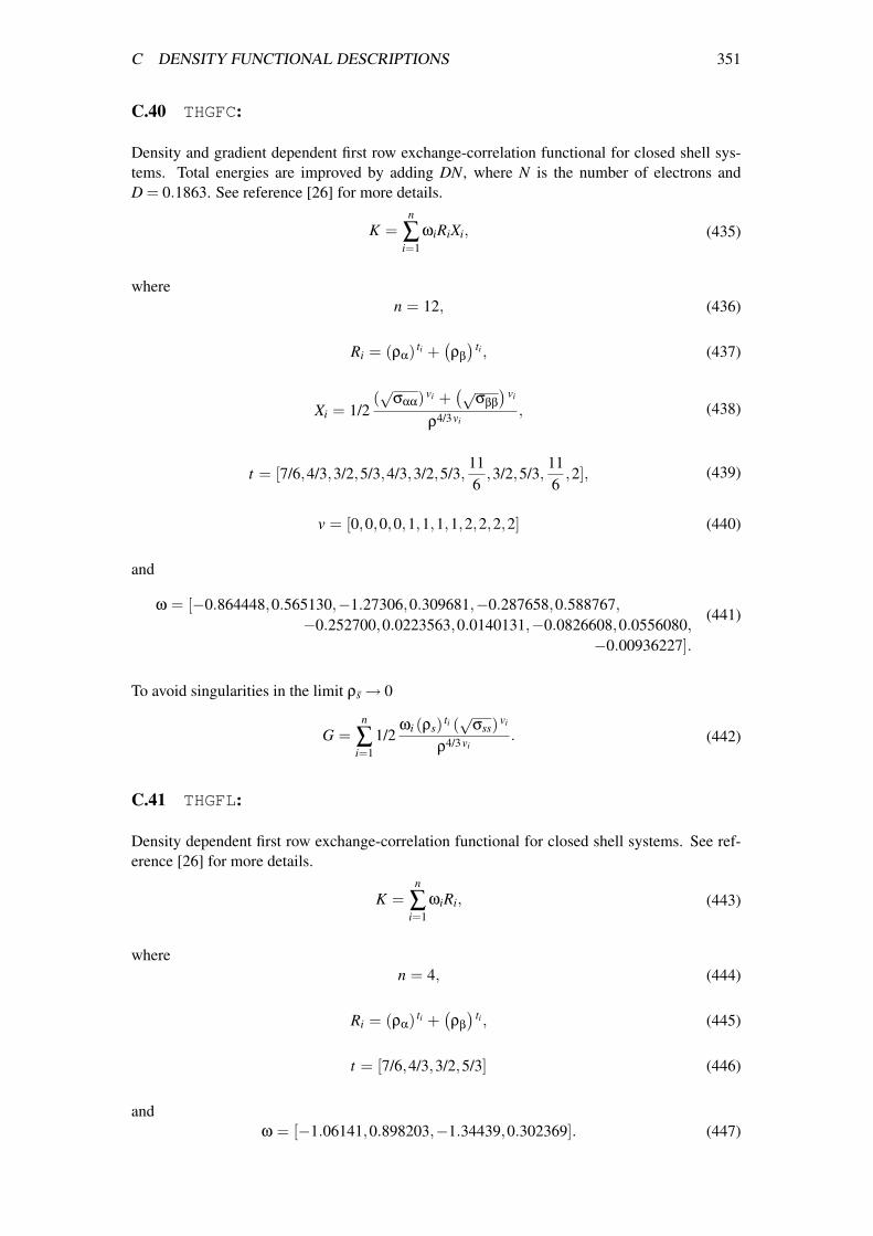
C DENSITY FUNCTIONAL DESCRIPTIONS 351
C.40 THGFC:
Density and gradient dependent first row exchange-correlation functional for closed shell sys-tems. Total energies are improved by adding DN, where N is the number of electrons andD = 0.1863. See reference [26] for more details.
(435)K =n
∑i=1
ωiRiXi,
where(436)n = 12,
(437)Ri = (ρα) ti +(ρβ
) ti ,
(438)Xi = 1/2(√
σαα) vi +(√
σββ
)vi
ρ4/3vi,
(439)t = [7/6,4/3,3/2,5/3,4/3,3/2,5/3,116
,3/2,5/3,116
,2],
(440)v = [0,0,0,0,1,1,1,1,2,2,2,2]
and
(441)ω = [−0.864448,0.565130,−1.27306,0.309681,−0.287658,0.588767,
−0.252700,0.0223563,0.0140131,−0.0826608,0.0556080,
−0.00936227].
To avoid singularities in the limit ρs → 0
(442)G =n
∑i=1
1/2ωi (ρs) ti (
√σss) vi
ρ4/3vi.
C.41 THGFL:
Density dependent first row exchange-correlation functional for closed shell systems. See ref-erence [26] for more details.
(443)K =n
∑i=1
ωiRi,
where(444)n = 4,
(445)Ri = (ρα) ti +(ρβ
) ti ,
(446)t = [7/6,4/3,3/2,5/3]
and(447)ω = [−1.06141,0.898203,−1.34439,0.302369].

C DENSITY FUNCTIONAL DESCRIPTIONS 352
C.42 VSXC:
See reference [27] for more details.
K = F (x,z, p3,q3,r3, t3,u3,v3,α3)(ε(ρα,ρβ
)− ε(ρα,0)− ε
(ρβ,0
))+ ∑
s(ρs) 4/3F (χs,zs, p1,q1,r1, t1,u1,v1,α1)
+ dsε(ρs,0)F (χs,zs, p2,q2,r2, t2,u2,v2,α2) ,(448)
where(449)x = (χα) 2 +
(χβ
) 2,
(450)zs =τs
(ρs) 5/3 − cf ,
(451)z =τα
(ρα) 5/3 +τβ(
ρβ
)5/3
− 2cf ,
(452)ds = 1 − (χs) 2
4zs + 4cf,
(453)F (x,z, p,q,c,d,e, f ,α) =p
λ(x,z,α)+
qx2 + cz(λ(x,z,α)) 2 +
dx4 + ex2z + f z2
(λ(x,z,α)) 3 ,
(454)λ(x,z,α) = 1 + α(x2 + z
),
(455)cf = 3/532/3 (π
2) 2/3,
ε(α,β) = (α + β)
(e(l (α,β) ,T1,U1,V1,W1,X1,Y1,P1)
−e(l (α,β) ,T3,U3,V3,W3,X3,Y3,P3)ω(ζ(α,β))
(1 − (ζ(α,β)) 4
)c
+(e(l (α,β) ,T2,U2,V2,W2,X2,Y2,P2)−e(l (α,β) ,T1,U1,V1,W1,X1,Y1,P1))ω(ζ(α,β))(ζ(α,β)) 4
),
(456)
(457)l (α,β) = 1/4 3√
342/3 3
√1
π (α + β),
(458)ζ(α,β) =α − β
α + β,
(459)ω(z) =(1 + z) 4/3 + (1 − z) 4/3 − 2
2 3√
2 − 2,
(460)e(r, t,u,v,w,x,y, p) = −2 t (1 + ur) ln(
1 + 1/21
t (v√
r + wr + xr3/2 + yrp+1)
),

C DENSITY FUNCTIONAL DESCRIPTIONS 353
(461)c = 1.709921,
(462)p = [−0.98,0.3271,0.7035],
(463)q = [−0.003557,−0.03229,0.007695],
(464)r = [0.00625,−0.02942,0.05153],
(465)t = [−0.00002354,0.002134,0.00003394],
(466)u = [−0.0001283,−0.005452,−0.001269],
(467)v = [0.0003575,0.01578,0.001296],
(468)α = [0.001867,0.005151,0.00305],
(469)T = [0.031091,0.015545,0.016887],
(470)U = [0.21370,0.20548,0.11125],
(471)V = [7.5957,14.1189,10.357],
(472)W = [3.5876,6.1977,3.6231],
(473)X = [1.6382,3.3662,0.88026],
(474)Y = [0.49294,0.62517,0.49671]
and(475)P = [1,1,1].
To avoid singularities in the limit ρs → 0
G = (ρs) 4/3F (χs,zs, p1,q1,r1, t1,u1,v1,α1) + dsε(ρs,0)F (χs,zs, p2,q2,r2, t2,u2,v2,α2) .(476)

C DENSITY FUNCTIONAL DESCRIPTIONS 354
C.43 VWN3: Vosko-Wilk-Nusair (1980) III local correlation energy
VWN 1980(III) functional. The fitting parameters for ∆εc(rs,ζ)III appear in the text shortly afterequation 4.4 of the reference. See reference [28] for more details.
(477)K = ρe,
where
(478)x = 1/4 6√
345/6 6
√1
πρ,
(479)ζ =ρα − ρβ
ρ,
(480)e = Λ + αy(1 + hζ
4) ,(481)y =
98
(1 + ζ) 4/3 +98
(1 − ζ) 4/3 − 9/4,
(482)h = 4/9λ − Λ(
3√
2 − 1)
α
− 1,
(483)Λ = q(k1, l1,m1,n1) ,
(484)λ = q(k2, l2,m2,n2) ,
(485)α = q(k3, l3,m3,n3) ,
q(A, p,c,d) = A(
ln(
x2
X (x,c,d)
)+ 2carctan
(Q(c,d)2x + c
)(Q(c,d))−1
− cp(
ln(
(x − p) 2
X (x,c,d)
)+ 2 (c + 2 p)arctan
(Q(c,d)2x + c
)(Q(c,d))−1
)(X (p,c,d))−1
),
(486)
(487)Q(c,d) =√
4d − c2,
(488)X (i,c,d) = i2 + ci + d,
(489)k = [0.0310907,0.01554535,−1/6π−2],
(490)l = [−0.409286,−0.743294,−0.0047584],
(491)m = [13.0720,20.1231,1.13107]
and(492)n = [42.7198,101.578,13.0045].

INDEX 355
C.44 VWN5: Vosko-Wilk-Nusair (1980) V local correlation energy
VWN 1980(V) functional. The fitting parameters for ∆εc(rs,ζ)V appear in the caption of table7 in the reference. See reference [28] for more details.
(493)K = ρe,
where
(494)x = 1/4 6√
345/6 6
√1
πρ,
(495)ζ =ρα − ρβ
ρ,
(496)e = Λ + αy(1 + hζ
4) ,(497)y =
98
(1 + ζ) 4/3 +98
(1 − ζ) 4/3 − 9/4,
(498)h = 4/9λ − Λ(
3√
2 − 1)
α
− 1,
(499)Λ = q(k1, l1,m1,n1) ,
(500)λ = q(k2, l2,m2,n2) ,
(501)α = q(k3, l3,m3,n3) ,
q(A, p,c,d) = A(
ln(
x2
X (x,c,d)
)+ 2carctan
(Q(c,d)2x + c
)(Q(c,d))−1
− cp(
ln(
(x − p) 2
X (x,c,d)
)+ 2 (c + 2 p)arctan
(Q(c,d)2x + c
)(Q(c,d))−1
)(X (p,c,d))−1
),
(502)
(503)Q(c,d) =√
4d − c2,
(504)X (i,c,d) = i2 + ci + d,
(505)k = [0.0310907,0.01554535,−1/6π−2],
(506)l = [−0.10498,−0.325,−0.0047584],
(507)m = [3.72744,7.06042,1.13107]
and(508)n = [12.9352,18.0578,13.0045].

INDEX 356
Index! (comments in input), 5***, 28, (comma), 5---, 5, 28; (end of input record), 5
ACCURACY, 97, 125ACPF, 136ACTIVE, 258ADD, 209, 244, 275, 287ALTERN, 232ANGULAR, 103AOINT, 69AQCC, 136arrays, 10Atomic mass, 75
BASIS, 79, 80basis
cartesian, 78spherical harmonic, 78
basis set, 77contraction, 84even tempered, 83primitive, 82
BCCD, 161BMAT, 257BRUECKNER, 161
CANONICAL, 120CANORB, 120CASPROJ, 231CASSCF, 112, 227CASVB, 227CCSD, 160CCSD, 131, 160CCSD(T), 160CEPA, 136CHARGE, 16CHECK, 160, 164CI, 131CI, 131CI-PRO, 131CIS, 168CIS, 168CISD, 162CISD, 131CIWEIGHTS, 235CLEAR, 53CLEARALL, 53
CLOSED, 16, 93, 114, 132COEFFS, 233COMPRESS, 69CON, 116, 135, 229CONFIG, 122CONICAL, 264COORD, 257coordinates, 257
B-matrix, 257cartesian, 257natural internal, 257Z-Matrix, 257
COPT, 126CORE, 16, 109, 132, 199COSMO, 284Cowan-Griffin, 212CPF, 136CPMCSCF, 128CPP, 87CRD, 73CRIT, 231CUBE, 213CUT, 262
Darwin, 212DATA, 14, 40DDR, 218DELETE, 39, 209DELOCAL, 108DELSTRUC, 234DEMC, 246DENSITY, 17, 100, 111, 206, 208, 210Density fitting, 65Density functionals
ALYP, 321B86, 322B86MGC, 321B86R, 322B88, 324B88C, 323B88CMASK, 322B95, 325B97, 327B97R, 326BW, 329CS1, 330CS2, 330DIRAC, 330G96, 330

INDEX 357
HCTH120, 331HCTH147, 332HCTH93, 333LTA, 335MK00, 336MK00B, 336P86, 336PBEC, 338PBEX, 340PBEXREV, 340PW86, 341PW91C, 341PW91X, 343PW92C, 344STEST, 344TH1, 345TH2, 346TH3, 347TH4, 348THGFC, 351THGFCFO, 349THGFCO, 350THGFL, 351VSXC, 352VWN3, 354VWN5, 355
Density matrices, 17DF-LMP2, 195DF-MP2, 158DFT, 99DFTBLOCK, 101DFTDUMP, 101DFTFACTOR, 100DFTTHRESH, 100Difference gradients, 128Diabatization, 221DIIS, 127, 162DIP, 210DIP+, 210dipole field, 210DIRECT, 56, 98distributed multipole analysis, 208DM, 124, 139, 158, 163DMA, 208DO, 29DO loops, 29DONT, 123DUMMY, 75Dummy-centres (Q,X), 71DUMP, 200
ECP
library, 85ECP, 84effective core potential, 84ELSEIF, 30ENDDO, 29ENDIF, 30ENDZ, 71EOM, 164EOM-CCSD, 164EOMPAR, 165EOMPRINT, 165ERASE, 39Examples, 22
allene_opt_bmat.com, 270allene_optmp2.com, 271allene_optscf.com, 270ar2_rel.com, 37, 89, 212auh_ecp_lib.com, 86bh_mrci_sigma_delta.com, 145caffeine_opt_diis.com, 271cn_sa_casscf.com, 130cndft.com, 106cu_ecp_explicit.com, 86field.com, 211form_freq.com, 282h2.com, 22h2f_merge.com, 290h2o_c2v_cs_start.com, 95h2o_caspt2_opt.com, 153h2o_casscf.com, 129h2o_ccsd.com, 162h2o_ccsdt_vtz.com, 23h2o_cepa1.com, 144h2o_diffden_molden.com, 74h2o_direct.com, 64h2o_dma.com, 209h2o_field.com, 211h2o_forces.com, 246h2o_gexpec1.com, 207h2o_gexpec2.com, 36h2o_manymethods.com, 26, 30h2o_mrcc.com, 173h2o_mrcc_eom.com, 173h2o_mrci_vtz.com, 23h2o_mscaspt2_opt.com, 154h2o_pes_ccsdt.com, 25, 30h2o_pop.com, 210h2o_proce.com, 25h2o_property.com, 207h2o_put_molden.com, 74h2o_scf.com, 22h2o_scf_vtz.com, 22, 79

INDEX 358
h2o_scf_vtz_explicit.com, 79h2o_scfopt_631g.com, 23h2o_sto3gstart1.com, 94h2o_sto3gstart2.com, 95h2o_table.com, 23h2o_vqz_fp.com, 84h2o_vqz_fp_explicit.com, 84h2o_xyzinput.com, 72h2op_mrci_trans.com, 144h2s_diab.com, 121, 216h2s_diab1.com, 222h2s_diab2.com, 224hcn_ccsd_ts.com, 273hcn_isomerization.com, 274hcn_mp2_ts.com, 272hcn_mrci_ts.com, 273hf_eom_conv.com, 168hf_eom_pes.com, 166hf_eom_prop.com, 167hfdimer_cpcopt1.com, 275hfdimer_cpcopt1_num.com, 277hfdimer_cpcopt2.com, 279i_ecp.com, 242lif_mr_mscaspt2.com, 150lif_nacme.com, 219lif_sr_mscaspt2.com, 149lih2+_S0T0.com, 266lih2_D0D1.com, 265matrop.com, 299matropfield.com, 300n2_rasscf.com, 130n2f2_ccsd.com, 162na2_ecp_cpp.com, 88no_merge1.com, 290no_merge2.com, 291o2_mrcc.com, 175oh_macros.com, 45oh_samcforce.com, 245ohar_bsse.com, 76pf5_freq.com, 282s_so.com, 241
EXCHANGE, 100EXPEC, 36, 97, 124, 139EXPEC2, 124Expectation values, 36Explicit correlation, 196Explicitly correlated methods, 196Expressions, 8EXTRA, 288
FCI, 199FIELD, 211
FIELD+, 211FILE, 39Files, 12FIXORB, 234FIXSTRUC, 234FOCK, 110, 138FORCE, 244FREEZE, 114FREQUENCIES, 280frequencies, 280
energy variables, 281FROZEN, 16, 113FULL, 235Full CI, 199
G1, 152Gaussian, 73GDIRECT, 56GENERAL, 208GEOMETRY, 70
Geometry files, 74Molpro-92 style, 73Writing CRD files, 73Writing Gaussian input, 73Writing MOLDEN input, 73Writing XMol files, 73XYZ input, 72Z-matrix, 71
geometry, 70geometry optimization, 251
automatic, 251conical intersection, 264convergence criteria, 252counterpoise correction, 275DIIS method, 251, 255energy variables, 263quadratic steepest descent method, 251,
256, 263rational function method, 251, 255saddle point, 256, 262transition state, 256, 262
GEXPEC, 36GOPENMOL, 214GOTO, 31GPARAM, 40GPRINT, 35gradients, 244GRADTYP, 244GRID, 101GRIDPRINT, 104GRIDSAVE, 103GRIDSYM, 103

INDEX 359
GRIDTHRESH, 101GROUP, 109, 234GTHRESH, 34GUESS, 230
Help, 21HESSELEM, 260HESSIAN, 258hessian, 258, 260
elements, 260model, 258numerical, 259
HF,options, 90HF-SCF, 90Hints, 1
IF, 30IF blocks, 30INACTIVE, 258INCLUDE, 5, 29Indexed Variables, 45INDIVIDUAL, 210INIT, 289input format, 5input structure, 12Integral-direct, 56integrals, 69INTOPT, 127Intrinsic functions, 9intrinsic reaction coordinate, 256, 263Introductory examples, 22IPOL, 98IPRINT, 125IRC, 256, 263IRREPS, 232Isotope mass, 75ITERATIONS, 122
Keywords, 18KS, 99KS-SCF, 99
LABEL, 31LATTICE, 74LIBMOL, 85libmol, 78library, 85LIMIT, 208LINEAR, 208LINESEARCH, 263LOCAL, 120Local correlation, 176LOCALI, 108
Localization space, 109LOCAO, 108LOCORB, 120loops, 14LQUANT, 117
Macros in string variables, 44MASS, 75Mass-velocity, 212Matrix operations, 293MATROP, 293MAXDAV, 138MAXITER, 97, 126, 137, 231MCSCF, 112MCSCF, 112, 245MEMORY, 29Memory allocation, 14MERGE, 287METHOD, 255MOLDEN, 73molpro, 1Molpro help, 21Molpro2000, 318Molpro2002, 317Molpro2006.1, 316Molpro98, 319molpro basis, 78MOVE, 287MP2, 158MP2-F12, 196MP2-R12, 196MP3, 158MP4, 158MPP, 2MPP systems, 2MPPX, 3Mulliken analysis, 209MULTI, 112MULTI, 112
NACM, 128, 246NACME, 128, 218NATORB, 119, 140, 163NELEC, 15NOCASPROJ, 231NOCHECK, 160, 164NOEXC, 136NOEXTRA, 123NOGPRINT, 35NOGRIDSAVE, 103NOGRIDSYM, 103Non-adiabatic coupling, 128, 218, 221NONLINEAR, 127

INDEX 360
NONUCLEAR, 208NOORDER, 110NOPAIR, 136NOSINGLE, 136NOSYMPROJ, 233NUMERICAL, 247, 261Numerical gradients, 247NUMHES, 259
OCC, 16, 93, 109, 113, 132, 199OFFDIAG, 109OFFSET, 288OPEN, 93OPTG, 251OPTIM, 232OPTION, 140, 156, 263ORB, 230ORBIT, 199ORBITAL, 17, 93, 108, 110, 118, 132, 206,
245, 287orbital localization, 108orbital manipulation, 287orbital spaces, 16Orbitals, 17orbitals
closedCI, 132MCSCF, 114
closed shell, 16core, 16
CI, 132FCI, 199
frozen, 17MCSCF, 113, 114
internal, 16CI, 132
occupied, 16CI, 132FCI, 199MCSCF, 113
ORBPERM, 231ORBPRINT, 98, 125ORBREL, 233ORTH, 98, 234, 289ORTHCON, 234
PAIR, 136PAIRS, 136, 234Parallel, 2PARAM, 141Plotting, 73POLARIZABILITY, 97POP, 209
population analysis, 209POTENTIAL, 100PRINT, 111, 125, 142, 200, 207, 236, 264,
289, 298PROC, 32Procedures, 32program structure, 12PROJECT, 137, 288properties, 206
CI, 139MCSCF, 123
PROPERTY, 206pseudopotential, 84PSPACE, 117, 138PUNCH, 40PUT, 73
QCI, 161QCI, 131QUAD, 210QUAD+, 210quadrupole field, 210
RADIAL, 102RADIUS, 209reaction path, 256, 263READ, 230READPUN, 12READVAR, 53records, 13REF, 133References, vREFSTATE, 135REL, 212Relativistic corrections, 212RELAX, 164RESTART, 14, 28RESTRICT, 115, 134RHF, 90RHF-SCF, 90RI-MP2, 158RKS, 99RKS-SCF, 99ROOT, 262ROTATE, 96, 118, 289RS2, 146RS2, 146RS2C, 146RS3, 146RS3, 146Running MOLPRO, 1
SADDLE, 231

INDEX 361
SAMC, 245SAPT, 201SAVE, 93, 108, 118, 119, 138, 229, 289SCALE, 244SCF, 90SCHMIDT, 289SCORR, 235SCS-MP2, 159SELECT, 116, 133SERVICE, 236SET, 41SHIFT, 97, 137SHOW, 53sorted integrals, 69SPECIAL, 237Special Variables, 47SPIN, 15SPINBASIS, 229START, 94, 117, 139, 229, 236STATE, 115, 135STATUS, 33STEP, 126, 262String variables, 43STRONG, 234STRUC, 230Summary of keywords, 18SYM, 96SYMELM, 232symmetry, 70
WF card, 15additional
MCSCF, 123SCF, 96
Integral program, 14SYMPROJ, 233System variables, 44
TABLE, 54Tables, 54TEST, 126THERMO, 281THRESH, 111, 127, 142, 160TRAN, 124TRAN2, 124TRANH, 137TRANS, 139, 164, 233TRNINT, 127TRUST, 262
UHF, 90UHF-SCF, 90UKS, 99UKS-SCF, 99
UNCOMPRESS, 69UPDATE, 260
VARIABLE, 263, 281variables, 41
Indexed, 45Introduction, 10Setting, 41Special, 47String, 43System, 44
VB, 227VB, 129VBDUMP, 127, 228VBWEIGHTS, 235Vector operations, 47vibrational frequencies, 280VORONOI, 103
wavefunction definition, 15WEIGHT, 115WF, 15, 93, 114, 132, 199WRITE, 236
XYZ, 72, 73
Z-matrix, 71ZMAT, 71