User’s Guide Version 16 - Meteorologisches Institut · PDF filePUMA User’s Guide...

PUMA

User’s Guide

Version 16

Klaus FraedrichSimon BlessingHartmut BorthEdilbert KirkTorben KunzFrank Lunkeit

Alastair McDonaldSilke Schubert

Frank Sielmann

2

The PUMA User’s Guide is a publication of the

Theoretical Meteorology at the Meteorological Institute of

the University of Hamburg.

Address:

Prof. Dr. Klaus Fraedrich

Meteorological Institute

KlimaCampus

University of Hamburg

Grindelberg 5

D-20144 Hamburg

Germany

Contact:

[email protected]

[email protected]

[email protected]

[email protected]

Contents

1 Installation 5

1.1 Quick Installation . . . . . . . . . . . . . . . . . . . . . . . . . . . . . . . . . . . 5

1.2 Most16 directory . . . . . . . . . . . . . . . . . . . . . . . . . . . . . . . . . . . 5

1.3 Model build phase . . . . . . . . . . . . . . . . . . . . . . . . . . . . . . . . . . 6

1.4 Model run phase . . . . . . . . . . . . . . . . . . . . . . . . . . . . . . . . . . . 7

1.5 Running long simulations . . . . . . . . . . . . . . . . . . . . . . . . . . . . . . . 7

2 Introduction 9

2.1 Training of junior scientists and students . . . . . . . . . . . . . . . . . . . . . . 9

2.2 Compatibility with other models . . . . . . . . . . . . . . . . . . . . . . . . . . . 9

2.3 Scientific applications . . . . . . . . . . . . . . . . . . . . . . . . . . . . . . . . . 10

2.4 Requirements . . . . . . . . . . . . . . . . . . . . . . . . . . . . . . . . . . . . . 10

2.5 History . . . . . . . . . . . . . . . . . . . . . . . . . . . . . . . . . . . . . . . . . 10

3 Horizontal Grid 13

4 Modules 15

4.1 fftmod.f90 / fft991mod.f90 . . . . . . . . . . . . . . . . . . . . . . . . . . . . . . 15

4.2 guimod.f90 / guimod stub.f90 . . . . . . . . . . . . . . . . . . . . . . . . . . . . 16

4.3 legsym.f90 . . . . . . . . . . . . . . . . . . . . . . . . . . . . . . . . . . . . . . . 17

4.4 mpimod.f90 / mpimod stub.f90 . . . . . . . . . . . . . . . . . . . . . . . . . . . 18

4.5 puma.f90 . . . . . . . . . . . . . . . . . . . . . . . . . . . . . . . . . . . . . . . . 20

4.6 pumamod.f90 . . . . . . . . . . . . . . . . . . . . . . . . . . . . . . . . . . . . . 22

4.7 restartmod.f90 . . . . . . . . . . . . . . . . . . . . . . . . . . . . . . . . . . . . . 23

5 Parallel Program Execution 25

5.1 Concept . . . . . . . . . . . . . . . . . . . . . . . . . . . . . . . . . . . . . . . . 25

5.2 Parallelization in the Gridpoint Domain . . . . . . . . . . . . . . . . . . . . . . 25

5.3 Parallelization in the Spectral Domain . . . . . . . . . . . . . . . . . . . . . . . 26

5.4 Synchronization points . . . . . . . . . . . . . . . . . . . . . . . . . . . . . . . . 26

5.5 Source code . . . . . . . . . . . . . . . . . . . . . . . . . . . . . . . . . . . . . . 26

6 Graphical User Interface 29

6.1 Graphical user interface (GUI) . . . . . . . . . . . . . . . . . . . . . . . . . . . . 29

6.2 GUI configuration . . . . . . . . . . . . . . . . . . . . . . . . . . . . . . . . . . . 31

6.2.1 Array . . . . . . . . . . . . . . . . . . . . . . . . . . . . . . . . . . . . . 32

6.2.2 Plot . . . . . . . . . . . . . . . . . . . . . . . . . . . . . . . . . . . . . . 32

6.2.3 Palette . . . . . . . . . . . . . . . . . . . . . . . . . . . . . . . . . . . . . 33

6.2.4 Title . . . . . . . . . . . . . . . . . . . . . . . . . . . . . . . . . . . . . . 33

6.2.5 Geometry . . . . . . . . . . . . . . . . . . . . . . . . . . . . . . . . . . . 33

3

4 CONTENTS

7 Postprocessor Pumaburner 357.1 Introduction . . . . . . . . . . . . . . . . . . . . . . . . . . . . . . . . . . . . . . 357.2 Installation / Compilation . . . . . . . . . . . . . . . . . . . . . . . . . . . . . . 357.3 Usage . . . . . . . . . . . . . . . . . . . . . . . . . . . . . . . . . . . . . . . . . 367.4 Namelist . . . . . . . . . . . . . . . . . . . . . . . . . . . . . . . . . . . . . . . . 367.5 HTYPE . . . . . . . . . . . . . . . . . . . . . . . . . . . . . . . . . . . . . . . . 367.6 VTYPE . . . . . . . . . . . . . . . . . . . . . . . . . . . . . . . . . . . . . . . . 377.7 MODLEV . . . . . . . . . . . . . . . . . . . . . . . . . . . . . . . . . . . . . . . 377.8 hPa . . . . . . . . . . . . . . . . . . . . . . . . . . . . . . . . . . . . . . . . . . . 377.9 LATS and LONS . . . . . . . . . . . . . . . . . . . . . . . . . . . . . . . . . . . 377.10 MEAN . . . . . . . . . . . . . . . . . . . . . . . . . . . . . . . . . . . . . . . . . 387.11 Format of output data . . . . . . . . . . . . . . . . . . . . . . . . . . . . . . . . 387.12 SERVICE format . . . . . . . . . . . . . . . . . . . . . . . . . . . . . . . . . . . 387.13 HHMM . . . . . . . . . . . . . . . . . . . . . . . . . . . . . . . . . . . . . . . . 397.14 HEAD7 . . . . . . . . . . . . . . . . . . . . . . . . . . . . . . . . . . . . . . . . 397.15 MARS . . . . . . . . . . . . . . . . . . . . . . . . . . . . . . . . . . . . . . . . . 397.16 MULTI . . . . . . . . . . . . . . . . . . . . . . . . . . . . . . . . . . . . . . . . . 397.17 Namelist example . . . . . . . . . . . . . . . . . . . . . . . . . . . . . . . . . . . 407.18 Troubleshooting . . . . . . . . . . . . . . . . . . . . . . . . . . . . . . . . . . . . 40

8 Graphics 418.1 GrADS . . . . . . . . . . . . . . . . . . . . . . . . . . . . . . . . . . . . . . . . . 41

9 Model Dynamics 459.1 Model equations and numerics . . . . . . . . . . . . . . . . . . . . . . . . . . . . 459.2 Parameterizations . . . . . . . . . . . . . . . . . . . . . . . . . . . . . . . . . . . 47

9.2.1 Friction . . . . . . . . . . . . . . . . . . . . . . . . . . . . . . . . . . . . 479.2.2 Diabatic heating . . . . . . . . . . . . . . . . . . . . . . . . . . . . . . . 479.2.3 Diffusion . . . . . . . . . . . . . . . . . . . . . . . . . . . . . . . . . . . . 48

9.3 Scaling of Variables . . . . . . . . . . . . . . . . . . . . . . . . . . . . . . . . . . 509.4 Vertical Discretization . . . . . . . . . . . . . . . . . . . . . . . . . . . . . . . . 509.5 PUMA Flow Diagram . . . . . . . . . . . . . . . . . . . . . . . . . . . . . . . . 519.6 Initialization . . . . . . . . . . . . . . . . . . . . . . . . . . . . . . . . . . . . . . 519.7 Computations in spectral domain . . . . . . . . . . . . . . . . . . . . . . . . . . 52

10 Preprocessor 55

11 Benchmark 5711.1 Performance . . . . . . . . . . . . . . . . . . . . . . . . . . . . . . . . . . . . . . 57

A List of Constants and Symbols 61

B PUMA Codes for Variables 65

C Namelist 67

Chapter 1

Installation

The whole package, containing the models “Planet Simulator” and “PUMA” along with themodel starter “most” comes in a single file named “Most16.tgz” with 16 specifying the versionnumber. The following subsection shows the commands to use for installation:

1.1 Quick Installation

tar -zxvf Most16.tgz

cd Most16

./configure.sh

./most.x

If your tar command doesn’t support the “-z” option (e.g. on Sun UNIX), instead type:

gunzip Most16.tgz

tar -xvf Most16.tar

cd Most16

./configure.sh

./most.x

If this sequence of commands produces error messages, consult the FAQ (Frequently AskedQuestions) and the README files in the Most16 directory. They are in plain text files thatcan be read with the more command or any other text editor.

1.2 Most16 directory

home/Most16> ls -lg

-rw-r--r-- 3730 FAQ <- Frequently Asked Questions

-rw-r--r-- 7862 NEW_IN_VERSION_16 <- New in this version

-rw-r--r-- 718 README <- Read this first

-rw-r--r-- 168 README_MAC_USER <- Notes for MAC user

-rw-r--r-- 698 README_WINDOWS_USER <- Notes for Windows user

-rw-r--r-- 1548 cc_check.c <- Used by configure script

-rwxr-xr-x 57 cleanplasim <- Empty run, bld and bin for PLASIM

-rwxr-xr-x 51 cleanpuma <- Empty run, bld and bin for PUMA

-rwxr-xr-x 48 cleansam <- Empty run, bld and bin for SAM

-rwxr-xr-x 161 cmdpuma <- Build GUI-less PUMA

5

6 CHAPTER 1. INSTALLATION

-rwxr-xr-x 5611 configure.sh <- Configure script

-rw-r--r-- 308 csub.c <- Used by configure script

-rw-r--r-- 234 f90check.f90 <- Used by configure script

drwxr-xr-x 102 images <- Most images

-rw-r--r-- 81 make_most <- Used by configure script

-rw-r--r-- 154 makecheck <- Used by configure script

-rw-r--r-- 108 makedebug <- Used by configure script

-rw-r--r-- 84 makefile <- Makefile for building most.x

-rw-r--r-- 113461 most.c <- C source code for most

drwxr-xr-x 306 plasim <- Planet Simulator directory tree

drwxr-xr-x 238 postprocessor <- Postprocessor source and docs

drwxr-xr-x 306 puma <- PUMA directory tree

drwxr-xr-x 510 sam <- SAM directory tree

drwxr-xr-x 680 tools <- Some tools

The directory structure must not be changed! Even empty directories must be kept as theyare, because the Most program relies on their existence!

For each model, currently “Planet Simulator”, “SAM”, and “PUMA”, a directory exists(plasim or sam or puma) with the following subdirectories:

Most16/puma> ls -lg

drwxr-xr-x 2 128 bin <- model executables

drwxr-xr-x 2 1824 bld <- build directory

drwxr-xr-x 2 280 dat <- initial and boundary data

drwxr-xr-x 2 80 doc <- documentation, user’s guide, reference manual

drwxr-xr-x 2 928 run <- run directory

drwxr-xr-x 2 1744 src <- source code

After installation only “dat”, “doc” and “src” contain files. All other directories are empty.“MoSt” (the executable is named most.x) is used to define parameters, build the model,

create a runscript and optional start the model. The directories of the model are used in thefollowing manner:

1.3 Model build phase

Most writes an executable shell script to the “bld” directory and then executes it. First, itcopies all necessary source files from “src” to “bld” and modifies them according to the selectedparameter configuration. Modification of source code is necessary for vertical and horizontalresolution changes, and when using more than one processor (parallel program execution). Theoriginal files in the “src“ directory are not changed by MoSt.

The program modules are then compiled and linked using the make command, also issuedby MoSt. MoSt provides two different makefiles: one for the single CPU version and the otherfor the parallel version (using MPI, the Message Passing Interface). For Planet Simulator theresolution and CPU parameters are coded into the filename of the executable, in order thatthere are different names for different versions. E.g. the executable “most plasim t21 l10 p2.x”is an executable compiled for a horizontal resolution of T21, a vertical resolution of 10 levels and2 CPU’s. PUMA and SAM use universal executables, that can be used for different resolutions,because they use dynamical array allocation at runtime.

1.4. MODEL RUN PHASE 7

The executable is copied to the model’s “bin” directory at the end of the build. Rebuildingmay be forced by using the cleanpuma command in the most directory. The build directory isnot cleared after usage. The user may want to modify the makefile or the build script for hisown purposes and start the building directly by executing the “most puma build” script. Forpermanent user modifications, the contents of the “bld” directory has to be copied elsewhere,because each usage of MoSt overwrites its contents.

1.4 Model run phase

After building the model with the selected configuration, MoSt writes or copies all the necessaryfiles to the model’s “run” directory. These are the executable, initial and boundary data,namelist files containing the parameter, and finally the run script itself. Depending on the exitselected from MoSt, either “Save & Exit” or “Run & Exit”, the run script is started from MoStand takes control of the model run. A checkmark on GUI invokes the Graphical User Interfaceallowing the user to control and display variables during the run. Again, all the contents of the“run” directory are subject to change by the user. However, it is better to save the changed runsetups in other user-created directories, because each usage of MoSt will overwrite the contentsof the run directory. Alternatively, the user changed files could be renamed, because MoStalways generates files with names beginning with “most ” and leaves any other files untouched.

1.5 Running long simulations

For long simulations create a new directory on a file system that has enough free disk space tostore the results. You can use the “df” command to check file systems.

Hint 1: Do not use your home directory if there are file quotas. Your run may crash due tofile quota being exceeded.

Hint 2: If possible use a local disk, not a NFS mounted file system. The model runs muchfaster when writing output to local disks.

Example:

• cd Most16

• ./most.x

• Select model and resolution

• Switch GUI off

• Switch Output on

• Edit number of years to run

• Click on “Save & Exit”

• Make a directory, e.g. mkdir /data/longsim

• cp puma/run/* /data/longsim

• cd /data/longsim

• Edit the experiment name in most puma run

• Edit the namelist files if necessary

• Start the simulation with most puma run &

8 CHAPTER 1. INSTALLATION

Chapter 2

Introduction

The Portable University Model of the Atmosphere (PUMA) is based on the multi-level spec-tral model SGCM (Simple Global Circulation Model) described by [Hoskins and Simmons,1975] and [James and Gray, 1986]. Originally developed as a numerical prediction model, it waschanged to perform as a circulation model. For example, [James and Gray, 1986] studied theinfluence of surface friction on the circulation of a baroclinic atmosphere, [James and James,1992] and [James et al., 1994] investigated ultra-low-frequency variability, and [Mole and James,1990] analyzed the baroclinic adjustment in the context of a zonally varying flow. [Frisius et al.,1998] simulated an idealized storm track by embedding a dipole structure in a zonally symmetricforcing field and [Lunkeit et al., 1998] investigated the sensitivity of GCM scenarios by using anadaption technique applicable to SGCMs. Storm track dynamics and low frequency variabilitywas investigated by [Fraedrich et al., 2005]. For further citations search the bibliography at theend of this document and the list of publications at http://www.mi.uni-hamburg.de/puma.

PUMA was created with following aims in mind: training of junior scientists, compatibilitywith the ECHAM (European Centre - HAMburg) model and as a tool for further scientificinvestigations.

2.1 Training of junior scientists and students

PUMA contains only the main processes necessary to simulate the atmosphere. The sourcecode is short and clearly arranged. A student can learn to work with PUMA within a fewweeks, whereas a full size GCM requires a team of specialists for maintenance, experimentdesign and diagnostics.

2.2 Compatibility with other models

PUMA is designed to be compatible with other circulation models like Planet Simulator andECHAM. The same triangular truncation is employed, and analogous transformation techniqueslike the Legendre- and Fast-Fourier transformation are used. The postprocessor Pumaburnerdiffers from ECHAM’s Afterburner only in respect to the format of the model’s raw datawhich overcomes some problems of the ECHAM data format. PUMA uses a more compactthough more precise format compared to the GRIB (GRIdded Binary), which is used forECHAM output. The Pumaburner supports the output formats SERVICE and NetCDF. Alldiagnostics and graphics software that are used with the ECHAM/Afterburner data can beused with PUMA/Pumaburner in exactly the same way.

9

http://www.mi.uni-hamburg.de/puma

10 CHAPTER 2. INTRODUCTION

2.3 Scientific applications

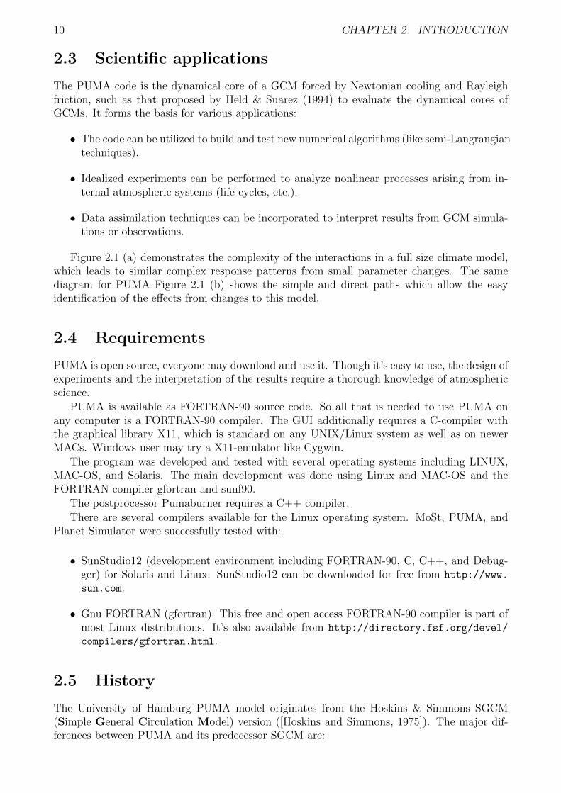
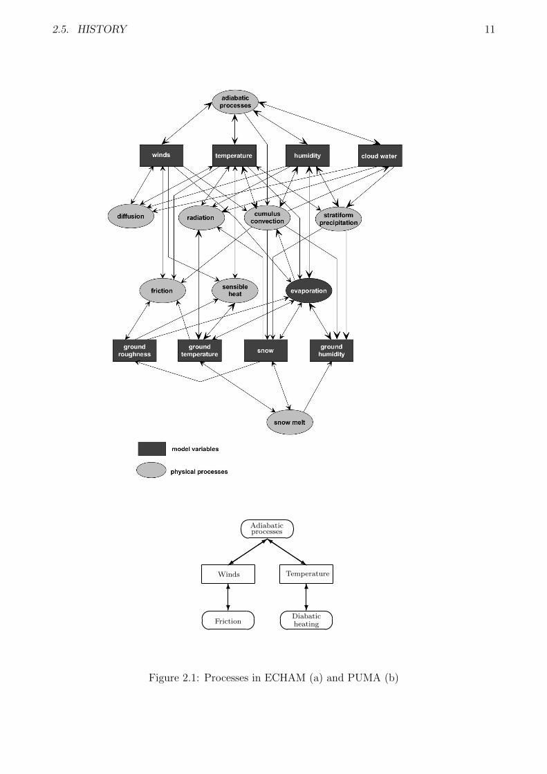
The PUMA code is the dynamical core of a GCM forced by Newtonian cooling and Rayleighfriction, such as that proposed by Held & Suarez (1994) to evaluate the dynamical cores ofGCMs. It forms the basis for various applications:

• The code can be utilized to build and test new numerical algorithms (like semi-Langrangiantechniques).

• Idealized experiments can be performed to analyze nonlinear processes arising from in-ternal atmospheric systems (life cycles, etc.).

• Data assimilation techniques can be incorporated to interpret results from GCM simula-tions or observations.

Figure 2.1 (a) demonstrates the complexity of the interactions in a full size climate model,which leads to similar complex response patterns from small parameter changes. The samediagram for PUMA Figure 2.1 (b) shows the simple and direct paths which allow the easyidentification of the effects from changes to this model.

2.4 Requirements

PUMA is open source, everyone may download and use it. Though it’s easy to use, the design ofexperiments and the interpretation of the results require a thorough knowledge of atmosphericscience.

PUMA is available as FORTRAN-90 source code. So all that is needed to use PUMA onany computer is a FORTRAN-90 compiler. The GUI additionally requires a C-compiler withthe graphical library X11, which is standard on any UNIX/Linux system as well as on newerMACs. Windows user may try a X11-emulator like Cygwin.

The program was developed and tested with several operating systems including LINUX,MAC-OS, and Solaris. The main development was done using Linux and MAC-OS and theFORTRAN compiler gfortran and sunf90.

The postprocessor Pumaburner requires a C++ compiler.

There are several compilers available for the Linux operating system. MoSt, PUMA, andPlanet Simulator were successfully tested with:

• SunStudio12 (development environment including FORTRAN-90, C, C++, and Debug-ger) for Solaris and Linux. SunStudio12 can be downloaded for free from http://www.

sun.com.

• Gnu FORTRAN (gfortran). This free and open access FORTRAN-90 compiler is part ofmost Linux distributions. It’s also available from http://directory.fsf.org/devel/

compilers/gfortran.html.

2.5 History

The University of Hamburg PUMA model originates from the Hoskins & Simmons SGCM(Simple General Circulation Model) version ([Hoskins and Simmons, 1975]). The major dif-ferences between PUMA and its predecessor SGCM are:

http://www.sun.com

http://www.sun.com

http://directory.fsf.org/devel/compilers/gfortran.html

http://directory.fsf.org/devel/compilers/gfortran.html

2.5. HISTORY 11

Adiabaticprocesses

QQQQQsQQQ

QQk

+3

Winds Temperature

?

6

?

6

Friction

Diabaticheating

Figure 2.1: Processes in ECHAM (a) and PUMA (b)

12 CHAPTER 2. INTRODUCTION

• The code is rewritten in portable FORTRAN-90 code, which removes problems associ-ated with machine-specific properties like word lengths, floating point precision, output,etc. All the necessary routines are in the source code including the FFT (Fast FourierTransformation) and the Legendre Transformation. The model can be run on any com-puter with a standard FORTRAN-90 compiler. The MPI-library is needed to run PUMAon parallel machines (see below). The Xlib (X11R6) library is needed for the graphicaluser interface.

• The truncation scheme is changed from the jagged triangular truncation to the standardtriangular truncation scheme making it compatible to other T-models like ECHAM.

• The PUMA/Pumaburner system is data compatible to ECHAM/Afterburner. Thus allother ECHAM diagnostic software can be used on PUMA data.

• PUMA is fully parallelized and can use as many CPU’s as half of the number of latitudes(e.g. 16 in T21 resolution). It uses the MPI (Message Passing Interface) library whilerunning on parallel systems or a cluster. MPI is not needed for running PUMA on asingle CPU.

• The ongoing development added several new features like the preprocessor, graphical userinterface, spherical harmonics mode selection, and many more.

Chapter 3

Horizontal Grid

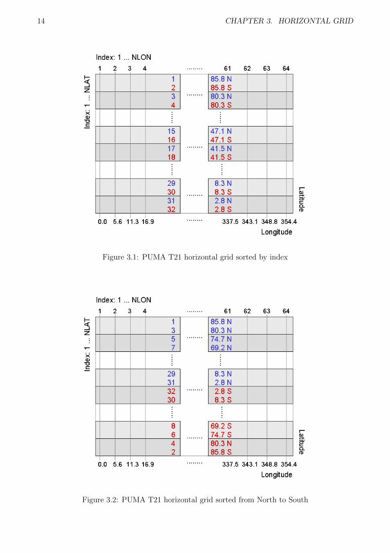
PUMA uses internally (other than the Planet Simulator and PUMA version 15) an alternatingGaussian grid. This feature is unimportant for users, who don’t change source code - the outputfile will still contain the usual Gaussian grid with the latitude index running from the mostNorthern latitude to the most Southern one. But for those, who fiddle around with the codeor want to implement additional arrays it is important to understand the internal structure.

The alternating grid was introduced for two reasons:1) The number of values for Legendre polynomials could be reduced by a factor of two,

because pairs of Northern and Southern latitudes with the same absolute value can be processedsimultaneously. This is especially useful for very high resolution runs. E.g. a PUMA T1365needs now ca. 45 GByte memory.

2) The Legendre transformation was recoded to use symmetric and antisymmetric Fouriercoefficients for these latitude pairs resulting in strict conservation of symmetry and antisym-metry properties.

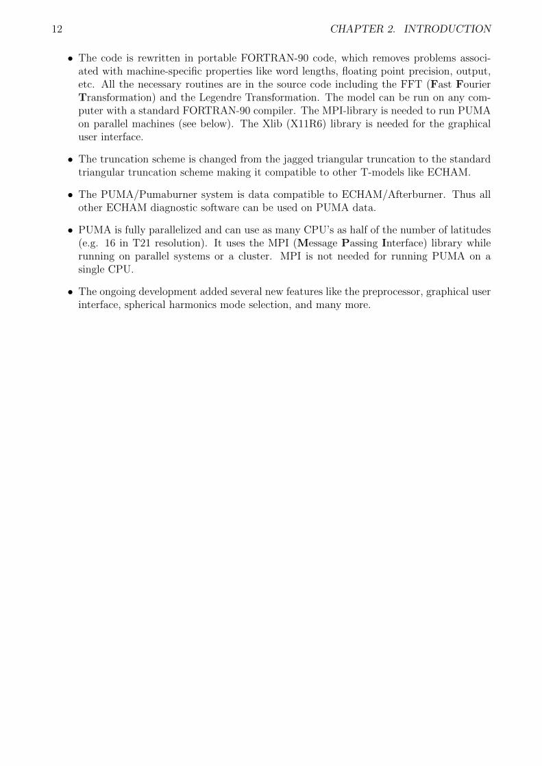
Figure 3.1 shows how the elements of a horizontal grid are stored in computer memory. Therestrictions for parallel execution using alternating grids are:

Because a latitude pair must not be separated to different processes, the maximum numberof processes is half of the number of latitudes. Also it not possible to use an odd number ofprocesses.

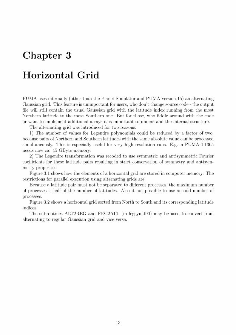
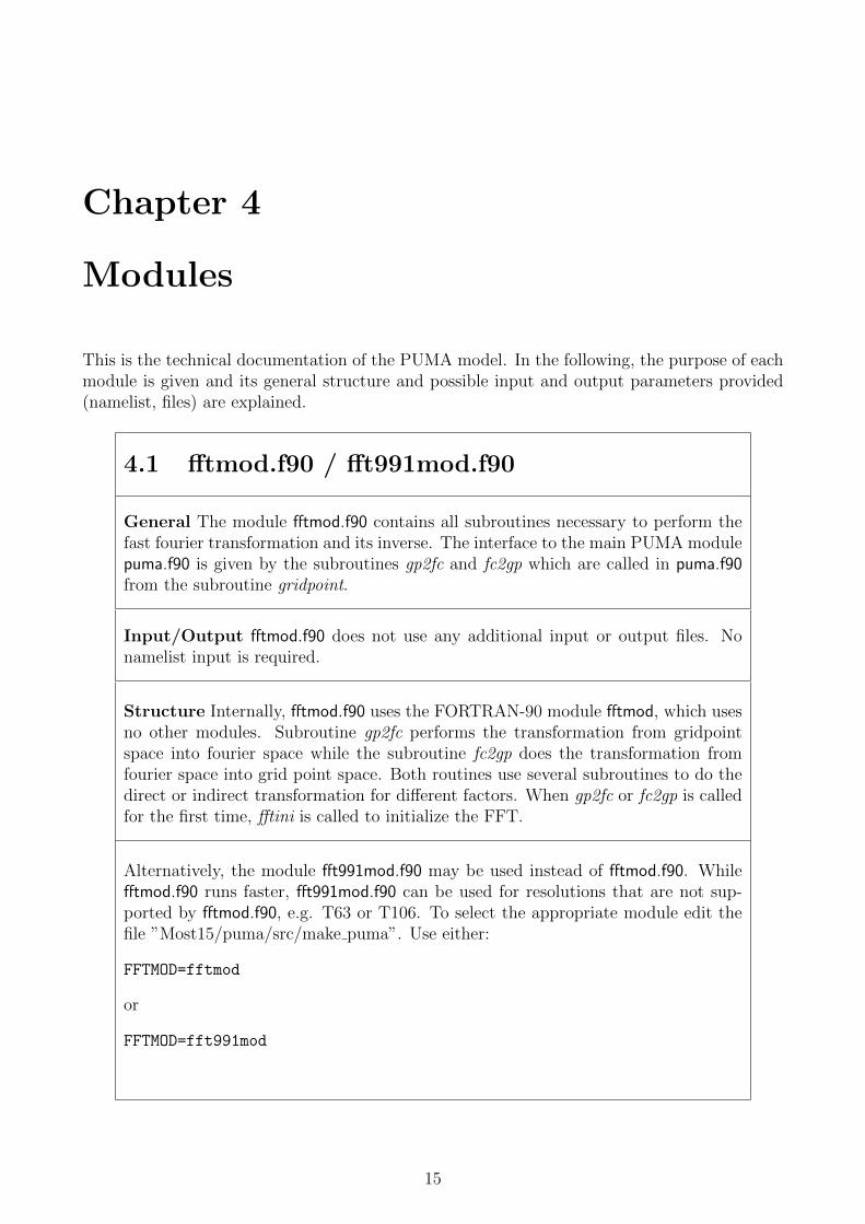
Figure 3.2 shows a horizontal grid sorted from North to South and its corresponding latitudeindices.

The subroutines ALT2REG and REG2ALT (in legsym.f90) may be used to convert fromalternating to regular Gaussian grid and vice versa.

13

14 CHAPTER 3. HORIZONTAL GRID

Figure 3.1: PUMA T21 horizontal grid sorted by index

Figure 3.2: PUMA T21 horizontal grid sorted from North to South

Chapter 4

Modules

This is the technical documentation of the PUMA model. In the following, the purpose of eachmodule is given and its general structure and possible input and output parameters provided(namelist, files) are explained.

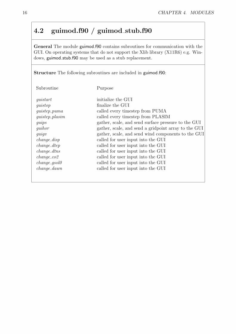
4.1 fftmod.f90 / fft991mod.f90

General The module fftmod.f90 contains all subroutines necessary to perform thefast fourier transformation and its inverse. The interface to the main PUMA modulepuma.f90 is given by the subroutines gp2fc and fc2gp which are called in puma.f90from the subroutine gridpoint.

Input/Output fftmod.f90 does not use any additional input or output files. Nonamelist input is required.

Structure Internally, fftmod.f90 uses the FORTRAN-90 module fftmod, which usesno other modules. Subroutine gp2fc performs the transformation from gridpointspace into fourier space while the subroutine fc2gp does the transformation fromfourier space into grid point space. Both routines use several subroutines to do thedirect or indirect transformation for different factors. When gp2fc or fc2gp is calledfor the first time, fftini is called to initialize the FFT.

Alternatively, the module fft991mod.f90 may be used instead of fftmod.f90. Whilefftmod.f90 runs faster, fft991mod.f90 can be used for resolutions that are not sup-ported by fftmod.f90, e.g. T63 or T106. To select the appropriate module edit thefile ”Most15/puma/src/make puma”. Use either:

FFTMOD=fftmod

or

FFTMOD=fft991mod

15

16 CHAPTER 4. MODULES

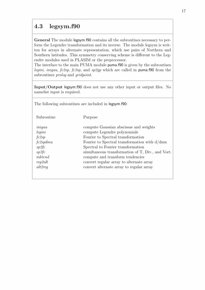
4.2 guimod.f90 / guimod stub.f90

General The module guimod.f90 contains subroutines for communication with theGUI. On operating systems that do not support the Xlib library (X11R6) e.g. Win-dows, guimod stub.f90 may be used as a stub replacement.

Structure The following subroutines are included in guimod.f90:

Subroutine Purpose

guistart initialize the GUIguistop finalize the GUIguistep puma called every timestep from PUMAguistep plasim called every timestep from PLASIMguips gather, scale, and send surface pressure to the GUIguihor gather, scale, and send a gridpoint array to the GUIguigv gather, scale, and send wind components to the GUIchange disp called for user input into the GUIchange dtep called for user input into the GUIchange dtns called for user input into the GUIchange co2 called for user input into the GUIchange gsol0 called for user input into the GUIchange dawn called for user input into the GUI

17

4.3 legsym.f90

General The module legsym.f90 contains all the subroutines necessary to per-form the Legendre transformation and its inverse. The module legsym is writ-ten for arrays in alternate representation, which use pairs of Northern andSouthern latitudes. This symmetry conserving scheme is different to the Leg-endre modules used in PLASIM or the preprocessor.The interface to the main PUMA module puma.f90 is given by the subroutineslegini, inigau, fc2sp, fc3sp, and sp2gp which are called in puma.f90 from thesubroutines prolog and gridpoint.

Input/Output legsym.f90 does not use any other input or output files. Nonamelist input is required.

The following subroutines are included in legsym.f90:

Subroutine Purpose

inigau compute Gaussian abscissae and weightslegini compute Legendre polynomialsfc2sp Fourier to Spectral transformationfc2spdmu Fourier to Spectral transformation with d/dmusp2fc Spectral to Fourier transformationsp3fc simultaneous transformation of T, Div., and Vort.mktend compute and transform tendenciesreg2alt convert regular array to alternate arrayalt2reg convert alternate array to regular array


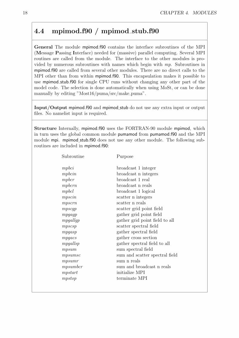
4.4 mpimod.f90 / mpimod stub.f90

General The module mpimod.f90 contains the interface subroutines of the MPI(Message Passing Interface) needed for (massive) parallel computing. Several MPIroutines are called from the module. The interface to the other modules is pro-vided by numerous subroutines with names which begin with mp. Subroutines inmpimod.f90 are called from several other modules. There are no direct calls to theMPI other than from within mpimod.f90. This encapsulation makes it possible touse mpimod stub.f90 for single CPU runs without changing any other part of themodel code. The selection is done automatically when using MoSt, or can be donemanually by editing ”Most16/puma/src/make puma”.

Input/Output mpimod.f90 and mpimod stub do not use any extra input or outputfiles. No namelist input is required.

Structure Internally, mpimod.f90 uses the FORTRAN-90 module mpimod, whichin turn uses the global common module pumamod from pumamod.f90 and the MPImodule mpi. mpimod stub.f90 does not use any other module. The following sub-routines are included in mpimod.f90:

Subroutine Purpose

mpbci broadcast 1 integermpbcin broadcast n integersmpbcr broadcast 1 realmpbcrn broadcast n realsmpbcl broadcast 1 logicalmpscin scatter n integersmpscrn scatter n realsmpscgp scatter grid point fieldmpgagp gather grid point fieldmpgallgp gather grid point field to allmpscsp scatter spectral fieldmpgasp gather spectral fieldmpgacs gather cross sectionmpgallsp gather spectral field to allmpsum sum spectral fieldmpsumsc sum and scatter spectral fieldmpsumr sum n realsmpsumbcr sum and broadcast n realsmpstart initialize MPImpstop terminate MPI

19

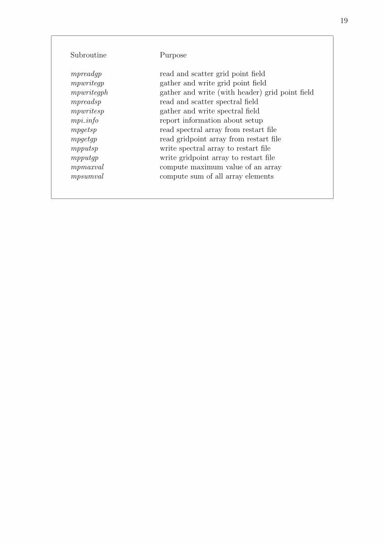
Subroutine Purpose

mpreadgp read and scatter grid point fieldmpwritegp gather and write grid point fieldmpwritegph gather and write (with header) grid point fieldmpreadsp read and scatter spectral fieldmpwritesp gather and write spectral fieldmpi info report information about setupmpgetsp read spectral array from restart filempgetgp read gridpoint array from restart filempputsp write spectral array to restart filempputgp write gridpoint array to restart filempmaxval compute maximum value of an arraympsumval compute sum of all array elements


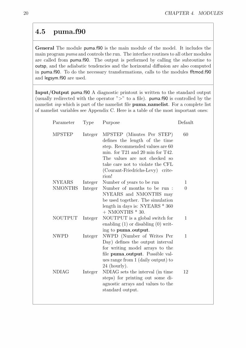
4.5 puma.f90

General The module puma.f90 is the main module of the model. It includes themain program puma and controls the run. The interface routines to all other modulesare called from puma.f90. The output is performed by calling the subroutine tooutsp, and the adiabatic tendencies and the horizontal diffusion are also computedin puma.f90. To do the necessary transformations, calls to the modules fftmod.f90and legsym.f90 are used.

Input/Output puma.f90 A diagnostic printout is written to the standard output(usually redirected with the operator ”>” to a file). puma.f90 is controlled by thenamelist inp which is part of the namelist file puma namelist. For a complete listof namelist variables see Appendix C. Here is a table of the most important ones:

Parameter Type Purpose Default

MPSTEP Integer MPSTEP (Minutes Per STEP)defines the length of the timestep. Recommended values are 60min. for T21 and 20 min for T42.The values are not checked sotake care not to violate the CFL(Courant-Friedrichs-Levy) crite-rion!

60

NYEARS Integer Number of years to be run 1NMONTHS Integer Number of months to be run :

NYEARS and NMONTHS maybe used together. The simulationlength in days is: NYEARS * 360+ NMONTHS * 30.

0

NOUTPUT Integer NOUTPUT is a global switch forenabling (1) or disabling (0) writ-ing to puma output.

1

NWPD Integer NWPD (Number of Writes PerDay) defines the output intervalfor writing model arrays to thefile puma output. Possible val-ues range from 1 (daily output) to24 (hourly).

1

NDIAG Integer NDIAG sets the interval (in timesteps) for printing out some di-agnostic arrays and values to thestandard output.

12

21

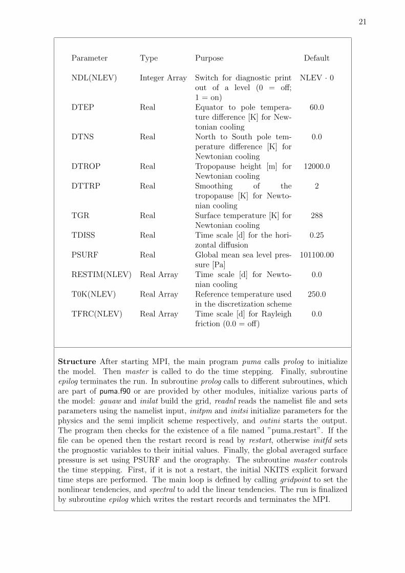
Parameter Type Purpose Default

NDL(NLEV) Integer Array Switch for diagnostic printout of a level (0 = off;1 = on)

NLEV · 0

DTEP Real Equator to pole tempera-ture difference [K] for New-tonian cooling

60.0

DTNS Real North to South pole tem-perature difference [K] forNewtonian cooling

0.0

DTROP Real Tropopause height [m] forNewtonian cooling

12000.0

DTTRP Real Smoothing of thetropopause [K] for Newto-nian cooling

2

TGR Real Surface temperature [K] forNewtonian cooling

288

TDISS Real Time scale [d] for the hori-zontal diffusion

0.25

PSURF Real Global mean sea level pres-sure [Pa]

101100.00

RESTIM(NLEV) Real Array Time scale [d] for Newto-nian cooling

0.0

T0K(NLEV) Real Array Reference temperature usedin the discretization scheme

250.0

TFRC(NLEV) Real Array Time scale [d] for Rayleighfriction (0.0 = off)

0.0

Structure After starting MPI, the main program puma calls prolog to initializethe model. Then master is called to do the time stepping. Finally, subroutineepilog terminates the run. In subroutine prolog calls to different subroutines, whichare part of puma.f90 or are provided by other modules, initialize various parts ofthe model: gauaw and inilat build the grid, readnl reads the namelist file and setsparameters using the namelist input, initpm and initsi initialize parameters for thephysics and the semi implicit scheme respectively, and outini starts the output.The program then checks for the existence of a file named ”puma restart”. If thefile can be opened then the restart record is read by restart, otherwise initfd setsthe prognostic variables to their initial values. Finally, the global averaged surfacepressure is set using PSURF and the orography. The subroutine master controlsthe time stepping. First, if it is not a restart, the initial NKITS explicit forwardtime steps are performed. The main loop is defined by calling gridpoint to set thenonlinear tendencies, and spectral to add the linear tendencies. The run is finalizedby subroutine epilog which writes the restart records and terminates the MPI.


4.6 pumamod.f90

General The module pumamod.f90 contains all the parameters and variables whichmay be used to share information between puma.f90 and other modules. No sub-routines or programs are included.

Input/Output pumamod.f90 does not use any extra input or output files. Nonamelist input is required.

Structure Internally, pumamod.f90 is a FORTRAN-90 module named pumamod.Names for global parameters, scalars and arrays are declared and, if possible, valuesare preset.

23

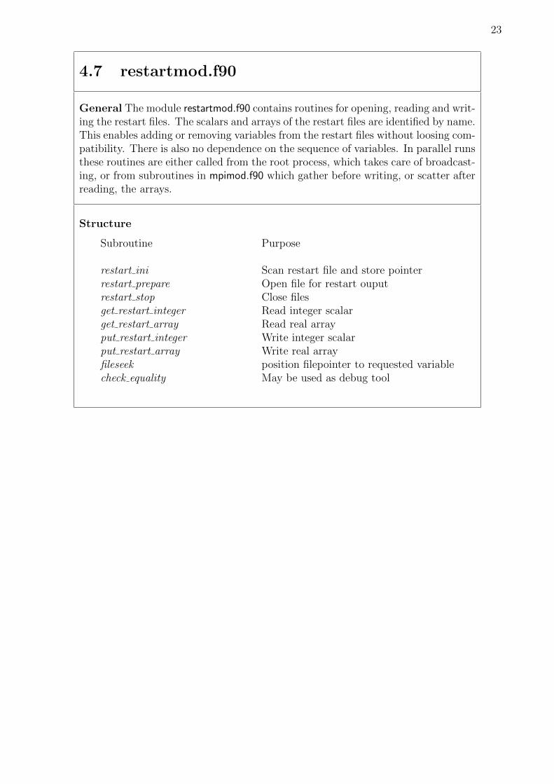
4.7 restartmod.f90

General The module restartmod.f90 contains routines for opening, reading and writ-ing the restart files. The scalars and arrays of the restart files are identified by name.This enables adding or removing variables from the restart files without loosing com-patibility. There is also no dependence on the sequence of variables. In parallel runsthese routines are either called from the root process, which takes care of broadcast-ing, or from subroutines in mpimod.f90 which gather before writing, or scatter afterreading, the arrays.

Structure

Subroutine Purpose

restart ini Scan restart file and store pointerrestart prepare Open file for restart ouputrestart stop Close filesget restart integer Read integer scalarget restart array Read real arrayput restart integer Write integer scalarput restart array Write real arrayfileseek position filepointer to requested variablecheck equality May be used as debug tool

Chapter 5

Parallel Program Execution

5.1 Concept

PUMA is coded for parallel execution on computers with multiple CPU’s or networked ma-chines. The implementation uses MPI (Message Passing Interface) that is available for nearlyevery operating system http://www.mcs.anl.gov/mpi.

In order to avoid maintaining two sets of source code for the parallel and the single CPUversion, all calls to the MPI routines are encapsulated into a module. Most takes care ofchoosing the correct version for compiling.

If MPI is not located by the configure script or the single CPU version is sufficient, thenthe module mpimod dummy.f90 is used instead of mpimod.f90.

5.2 Parallelization in the Gridpoint Domain

The data arrays in the gridpoint domain are either three-dimensional e.g. gt(NLON, NLAT,NLEV) referring to an array organized after longitudes, latitudes and levels, or two-dimensional,e.g. gp(NLON, NLAT). The code is organized so that there are no dependencies in the lat-itudinal direction while in the gridpoint domain. Such dependencies are resolved during theLegendre transformations. So the data is partitioned by latitude. The program can use asmany CPU’s as lf of the number of latitudes with each CPU doing the computations for apair of (North/South) latitudes. However, there is the restriction that the number of latitudes(NLAT) divided by the number of processors (NPRO), giving the number of latitudes per pro-cess (NLPP), must have zero remainder, e.g. a T31 resolution uses NLAT = 48. Possiblevalues for NPRO are then 1, 2, 3, 4, 6, 8, 12, and 24.

All loops dealing with a latitudinal index look like:

do jlat = 1 , NLPP

....

enddo

There are, however, many subroutines, with the most prominent called calcgp, that can fuselatitudinal and longitudinal indices. In all these cases the dimension NHOR is used. NHOR isdefined as: NHOR = NLON ∗NLPP in the pumamod - module. The typical gridpoint loop,which looks like:

do jlat = 1 , NLPP

do jlon = 1 , NLON

gp(jlon,jlat) = ...

enddo

25

http://www.mcs.anl.gov/mpi

26 CHAPTER 5. PARALLEL PROGRAM EXECUTION

enddo

is replaced by the faster executing loop:

do jhor = 1 , NHOR

gp(jhor) = ...

enddo

5.3 Parallelization in the Spectral Domain

The number of coefficients in the spectral domain (NRSP) is divided by the number of processes(NPRO) giving the number of coefficients per process (NSPP). The number is rounded up tothe next integer and the last process may get some additional dummy elements, if there is aremainder in the division operation.

All loops in spectral domain are organized like:

do jsp = 1 , NSPP

sp(jsp) = ...

enddo

5.4 Synchronization points

All processes must communicate and have therefore to be synchronized at following events:

• Legendre transformation: This involves changing from latitudinal partitioning to spectralpartitioning and associated gather and scatter operations.

• Inverse Legendre transformation: The partitioning changes from spectral to latitudinalby using gather, broadcast, and scatter operations.

• Input-Output: All read and write operations must only be performed by the root process,which gathers and broadcasts or scatters the desired information. Code that is to beexecuted by the root process exclusively is written as:

if (mypid == NROOT) then

...

endif

NROOT is typically 0 in MPI implementations, mypid (My process id) is assigned byMPI.

5.5 Source code

Discipline is required when maintaining parallel code. Here are the most important rules forchanging or adding code to PUMA:

• Adding namelist parameters: All namelist parameters must be broadcasted after readingthe namelist. (Subroutines mpbci, mpbcr, mpbcin, mpbcrn)

5.5. SOURCE CODE 27

• Adding scalar variables and arrays: Global variables must be defined in a module headerand initialized.

• Initialization code: Initialization code that contains dependencies on latitude or spectralmodes must be performed by the root process only and then scattered from there to allchild processes.

• Array dimensions and loop limits: Always use parameter constants (NHOR, NLAT,NLEV, etc.) as defined in pumamod.f90 for array dimensions and loop limits.

• Testing: After significant code changes the program should be tested in single and inmulti-CPU configurations. The results of a single CPU run is usually not exactly thesame as the result of a multi-CPU run due to effects in rounding. But the results shouldshow only small differences during the first few time steps.

• Synchronization points: The code is optimzed for parallel execution and therefore thecommunication overhead is minimized by grouping it around the Legendre transforma-tion. If more scatter/gather operations or other communication routines are to be added,they should be placed just before or after the execution of the calls to the Legendre trans-formation. Placing them elsewhere would degrade the overall performance by introducingadditional process synchronization.

28 CHAPTER 5. PARALLEL PROGRAM EXECUTION

Chapter 6

Graphical User Interface

6.1 Graphical user interface (GUI)

PUMA may be used in the traditional fashion, with shell scripts, batch jobs, and networkqueuing systems. This is useful for long running simulations on complex machines and num-ber crunchers, such as vector computers, massive parallel computers and workstation clusters.However, there is now a more convenient method. A graphical user interface (GUI) has beenprovided, which can be used for parameter configuration during model setup, and for interactionbetween the user and the model.

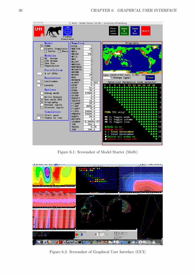
PUMA is setup and configured using the first GUI module named MoSt (Model Starter,screenshot in 6.1). MoSt is the fastest way to get the model running. It gives access to the mostimportant parameters of the model which are preset to the frequently used values. The modelcan be started with a mouse click on the button labelled “Save & Run” either with the standardparameter setting, or after editing the parameters in the MoSt window. Some parameters, likehorizontal and vertical resolution or the number of processors, require that a new executableis built (compile, link and load). MoSt achieves this by generating and executing build scripts,that perform the necessary code changes and create the required executables. Other parametersdefining startup and boundary conditions or other settings, can be edited with MoSt. Afterthey have been checked for correct range and for consistency with other parameters, they arewritten to the model’s namelist file.

Using these settings MoSt generates a run script for the simulation. The user then has thechoice of leaving MoSt and starting the simulation under the control of the GUI immediately,or of leaving MoSt with the scripts ready to run. This second alternative is useful for userswho want to include setup modifications beyond the scope of MoSt, or who want to run themodel without the GUI.

There is also a simple graphical editor for the topography. Check the box Orography andthen use the mouse to mark elliptic areas in the topographic display. Enter a value for raising(positive) or lowering (negative) the area and press the button labelled Preprocess. Thepreprocessor will be built and executed, and a new topography will be computed and writtento the start file.

Another editor is the Mode Editor for spherical harmonics. Green modes are enabled,red modes are disabled. This feature can be used to specify runs with only certain modes ofspherical harmonics being active. LMB, MMB and RMB refer to the left, middle, and rightmouse buttons respectively. You may toggle individual modes (press LMB) or whole lines (pressRMB) and columns (press MMB). Currently the Mode Editor can only be used for PUMA inthe T21 resolution.

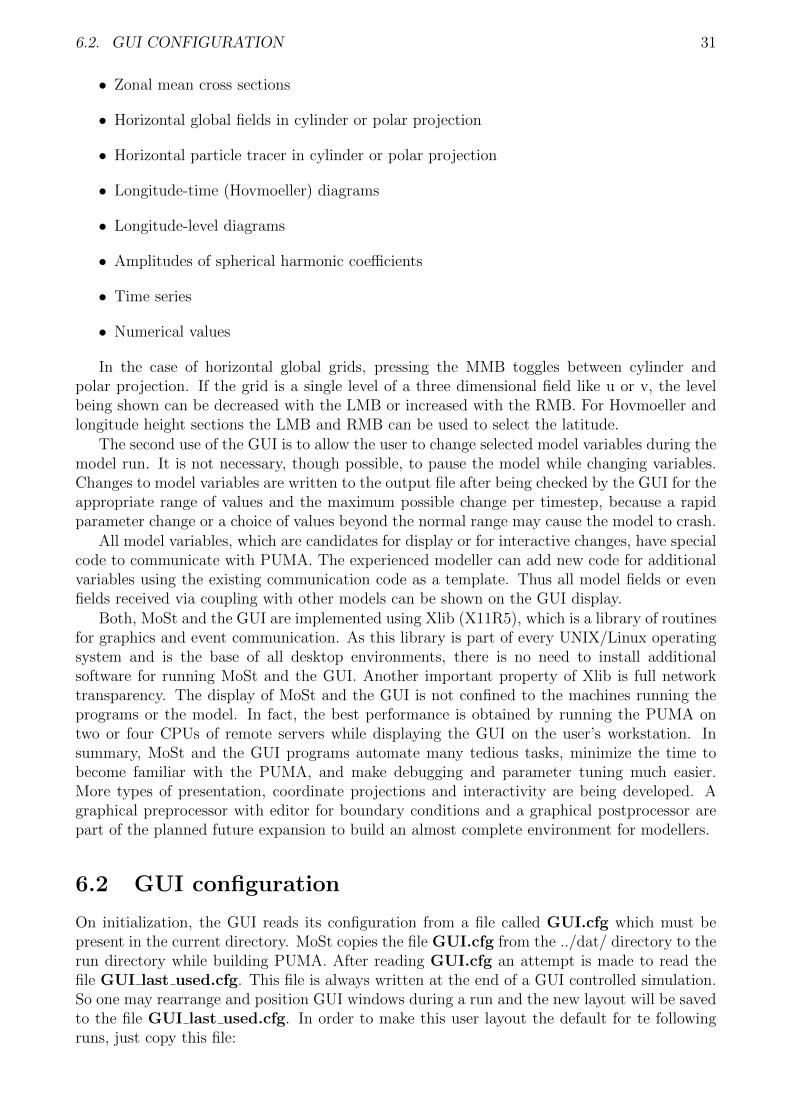
The GUI for running PUMA (Figure 6.2) has two main uses. The first is to display themodel arrays in suitable representations. Current implementations are:

29

30 CHAPTER 6. GRAPHICAL USER INTERFACE

Figure 6.1: Screenshot of Model Starter (MoSt)

Figure 6.2: Screenshot of Graphical User Interface (GUI)

6.2. GUI CONFIGURATION 31

• Zonal mean cross sections

• Horizontal global fields in cylinder or polar projection

• Horizontal particle tracer in cylinder or polar projection

• Longitude-time (Hovmoeller) diagrams

• Longitude-level diagrams

• Amplitudes of spherical harmonic coefficients

• Time series

• Numerical values

In the case of horizontal global grids, pressing the MMB toggles between cylinder andpolar projection. If the grid is a single level of a three dimensional field like u or v, the levelbeing shown can be decreased with the LMB or increased with the RMB. For Hovmoeller andlongitude height sections the LMB and RMB can be used to select the latitude.

The second use of the GUI is to allow the user to change selected model variables during themodel run. It is not necessary, though possible, to pause the model while changing variables.Changes to model variables are written to the output file after being checked by the GUI for theappropriate range of values and the maximum possible change per timestep, because a rapidparameter change or a choice of values beyond the normal range may cause the model to crash.

All model variables, which are candidates for display or for interactive changes, have specialcode to communicate with PUMA. The experienced modeller can add new code for additionalvariables using the existing communication code as a template. Thus all model fields or evenfields received via coupling with other models can be shown on the GUI display.

Both, MoSt and the GUI are implemented using Xlib (X11R5), which is a library of routinesfor graphics and event communication. As this library is part of every UNIX/Linux operatingsystem and is the base of all desktop environments, there is no need to install additionalsoftware for running MoSt and the GUI. Another important property of Xlib is full networktransparency. The display of MoSt and the GUI is not confined to the machines running theprograms or the model. In fact, the best performance is obtained by running the PUMA ontwo or four CPUs of remote servers while displaying the GUI on the user’s workstation. Insummary, MoSt and the GUI programs automate many tedious tasks, minimize the time tobecome familiar with the PUMA, and make debugging and parameter tuning much easier.More types of presentation, coordinate projections and interactivity are being developed. Agraphical preprocessor with editor for boundary conditions and a graphical postprocessor arepart of the planned future expansion to build an almost complete environment for modellers.

6.2 GUI configuration

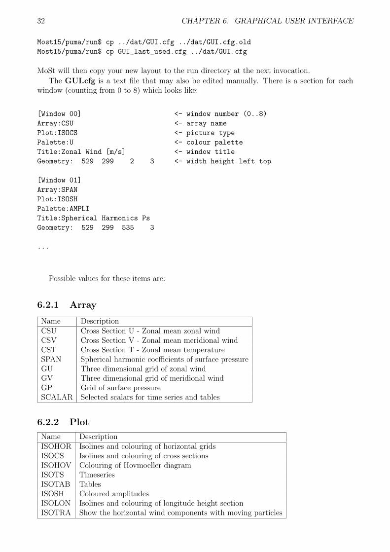
On initialization, the GUI reads its configuration from a file called GUI.cfg which must bepresent in the current directory. MoSt copies the file GUI.cfg from the ../dat/ directory to therun directory while building PUMA. After reading GUI.cfg an attempt is made to read thefile GUI last used.cfg. This file is always written at the end of a GUI controlled simulation.So one may rearrange and position GUI windows during a run and the new layout will be savedto the file GUI last used.cfg. In order to make this user layout the default for te followingruns, just copy this file:


Most15/puma/run$ cp ../dat/GUI.cfg ../dat/GUI.cfg.old

Most15/puma/run$ cp GUI_last_used.cfg ../dat/GUI.cfg

MoSt will then copy your new layout to the run directory at the next invocation.

The GUI.cfg is a text file that may also be edited manually. There is a section for eachwindow (counting from 0 to 8) which looks like:

[Window 00] <- window number (0..8)

Array:CSU <- array name

Plot:ISOCS <- picture type

Palette:U <- colour palette

Title:Zonal Wind [m/s] <- window title

Geometry: 529 299 2 3 <- width height left top

[Window 01]

Array:SPAN

Plot:ISOSH

Palette:AMPLI

Title:Spherical Harmonics Ps

Geometry: 529 299 535 3

...

Possible values for these items are:

6.2.1 Array

Name DescriptionCSU Cross Section U - Zonal mean zonal windCSV Cross Section V - Zonal mean meridional windCST Cross Section T - Zonal mean temperatureSPAN Spherical harmonic coefficients of surface pressureGU Three dimensional grid of zonal windGV Three dimensional grid of meridional windGP Grid of surface pressureSCALAR Selected scalars for time series and tables

6.2.2 Plot

Name DescriptionISOHOR Isolines and colouring of horizontal gridsISOCS Isolines and colouring of cross sectionsISOHOV Colouring of Hovmoeller diagramISOTS TimeseriesISOTAB TablesISOSH Coloured amplitudesISOLON Isolines and colouring of longitude height sectionISOTRA Show the horizontal wind components with moving particles

6.2. GUI CONFIGURATION 33

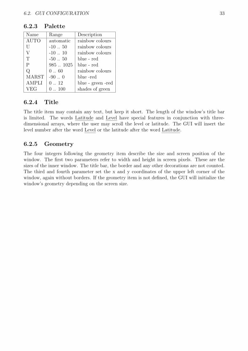
6.2.3 Palette

Name Range DescriptionAUTO automatic rainbow coloursU -10 .. 50 rainbow coloursV -10 .. 10 rainbow coloursT -50 .. 50 blue - redP 985 .. 1025 blue - redQ 0 .. 60 rainbow coloursMARST -90 .. 0 blue -redAMPLI 0 .. 12 blue - green -redVEG 0 .. 100 shades of green

6.2.4 Title

The title item may contain any text, but keep it short. The length of the window’s title baris limited. The words Latitude and Level have special features in conjunction with three-dimensional arrays, where the user may scroll the level or latitude. The GUI will insert thelevel number after the word Level or the latitude after the word Latitude.

6.2.5 Geometry

The four integers following the geometry item describe the size and screen position of thewindow. The first two parameters refer to width and height in screen pixels. These are thesizes of the inner window. The title bar, the border and any other decorations are not counted.The third and fourth parameter set the x and y coordinates of the upper left corner of thewindow, again without borders. If the geometry item is not defined, the GUI will initialize thewindow’s geometry depending on the screen size.

Chapter 7

Postprocessor Pumaburner

7.1 Introduction

The Pumaburner is a postprocessor for the Planet Simulator and the PUMA model family.It is the only interface between the raw model output data and the diagnostics, graphics, anduser software.

The output data of PUMA is stored as packed binary (16 bit) values using the modelrepresentation. Prognostic variables such as temperature, divergence, vorticity, pressure andhumidity are stored as coefficients of spherical harmonics on σ levels. Variables like radiation,precipitation, evaporation, clouds and other fields of the parameterization package are storedon Gaussian grids.

The tasks of the Pumaburner are:

• Unpack the raw data to full real representation.

• Transform variables from the model’s representation to a user selectable format, e.g. grids,zonal mean cross sections, and Fourier coefficients.

• Calculate diagnostic variables, such as vertical velocity, geopotential height, wind com-ponents, etc.

• Transfrom variables from σ levels to user selectable pressure levels.

• Compute monthly means and standard deviations.

• Write selected data either in SERVICE or NetCDF format for further processing.

7.2 Installation / Compilation

The Pumaburner doesn’t have to be installed, in most cases a compilation of the source codeand the storage of the executable in a ”bin” directory is sufficient. E.g.:

c++ -O2 -o burn6 burn6.cpp -lm -lnetcdf_c++ -lnetcdf

The NetCDF library version 3 or higher must be installed on the computer, otherwise theabove command will fail with an error. On some computer sites NetCDF might be installed,but the include or library search paths may lack the right configuration. In those cases eitherask your administrator to update the configuration or specify the necessary locations on thecompiler command using ”-I” to specify the path for ”Include” files and ”-L” for library files.Of course other C++ compilers, like g++ for example may be used as well. If you’re notthe admin of your system, put the executable burn6 into your $HOME/bin directory. This isnormally part of your search path.

35

36 CHAPTER 7. POSTPROCESSOR PUMABURNER

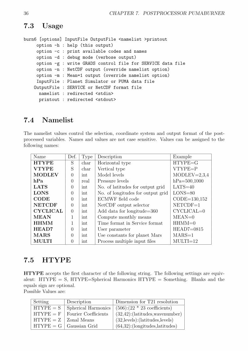
7.3 Usage

burn6 [options] InputFile OutputFile <namelist >printout

option -h : help (this output)

option -c : print available codes and names

option -d : debug mode (verbose output)

option -g : write GRADS control file for SERVICE data file

option -n : NetCDF output (override namelist option)

option -m : Mean=1 output (override namelist option)

InputFile : Planet Simulator or PUMA data file

OutputFile : SERVICE or NetCDF format file

namelist : redirected <stdin>

printout : redirected <stdout>

7.4 Namelist

The namelist values control the selection, coordinate system and output format of the post-processed variables. Names and values are not case sensitive. Values can be assigned to thefollowing names:

Name Def. Type Description ExampleHTYPE S char Horizontal type HTYPE=GVTYPE S char Vertical type VTYPE=PMODLEV 0 int Model levels MODLEV=2,3,4hPa 0 real Pressure levels hPa=500,1000LATS 0 int No. of latitudes for output grid LATS=40LONS 0 int No. of longitudes for output grid LONS=80CODE 0 int ECMWF field code CODE=130,152NETCDF 0 int NetCDF output selector NETCDF=1CYCLICAL 0 int Add data for longitude=360 CYCLICAL=0MEAN 1 int Compute monthly means MEAN=0HHMM 1 int Time format in Service format HHMM=0HEAD7 0 int User parameter HEAD7=0815MARS 0 int Use constants for planet Mars MARS=1MULTI 0 int Process multiple input files MULTI=12

7.5 HTYPE

HTYPE accepts the first character of the following string. The following settings are equiv-alent: HTYPE = S, HTYPE=Spherical Harmonics HTYPE = Something. Blanks and theequals sign are optional.Possible Values are:

Setting Description Dimension for T21 resolutionHTYPE = S Spherical Harmonics (506):(22 * 23 coefficients)HTYPE = F Fourier Coefficients (32,42):(latitudes,wavenumber)HTYPE = Z Zonal Means (32,levels):(latitudes,levels)HTYPE = G Gaussian Grid (64,32):(longitudes,latitudes)

7.6. VTYPE 37

7.6 VTYPE

VTYPE accepts the first character of the following string. The following settings are equiva-lent: VTYPE = S, VTYPE=Sigma, VTYPE = Super. Blanks and the equals sign are optional.Possible Values are:

Setting Description RemarkVTYPE = S Sigma (model) levels Some derived variables are not availableVTYPE = P Pressure levels Interpolation to pressure levels

7.7 MODLEV

MODLEV is used in combination with VTYPE = S. If VTYPE is not set to “Sigma”,the contents of MODLEV are ignored. MODLEV is an integer array that can have as manyvalues as there are levels in the model output. The levels are numbered from the top of theatmosphere to the bottom. The number of levels and the corresponding σ values are listed inthe Pumaburner printout. The levels are ordered in the output file according to the MODLEVvalues. MODLEV=1,2,3,4,5 produces an output file of five model levels sorted from top tobottom, while MODLEV=5,4,3,2,1 sorts them from bottom to top.

7.8 hPa

hPa is used in combination with VTYPE = P. If VTYPE is not set to “Pressure”, thecontents of hPa are ignored. hPa is a real array that accepts pressure values with the unitshectoPascal or millibar. All output variables will be interpolated to the selected pressure levels.There is no extrapolation at the top of the atmosphere. For pressure values, which are lowerthan that at the model’s top level, the top level value of the variable is taken. The variables,temperature and geopotential height, are extrapolated if the selected pressure is higher thanthe surface pressure. All other variables are set to the value of the lowest mode level for thiscase. The outputfile contains the levels in the same order as they are set in hPa. For example:hpa = 100,300,500,700,850,900,1000.

7.9 LATS and LONS

The Pumaburner defaults to the dimension of the model run. E.g. Lats = 32 and Lons = 64for a T21 resolution. Note however, that this results in Gaussian grids with non equidistantlatitudes. Selecting for Lats and Lons values, that are different from the internal resolutionproduces equidistant lat-lon grids. Lats sets the number of latitudes from north to south,with the North Pole at index 1 and the South Pole at index Lats. Delta Phi is therefore180 degrees / (Lats - 1). Lons sets the number of gridpoints on every latitude circle. DeltaLambda is 360 / Lons. Index 1 is on the Greewich Meridian (0 degrees), while the last indexdenotes the point (360 degrees - Delta Lambda). Technical note: Variables that are stored asspherical harmonics (Temperature, vorticity, divergence, etc.) are calculated on the user gridby setting up the Legendre Transformation and the FFT accordingly. Variables, that are storedon Gaussian grids are interpolated with a bilinear interpolation. Note: Lats >= 8 and Lons>= 16 due to technical reasons.


7.10 MEAN

MEAN can be used to compute monthly means and/or deviations. The Pumaburner readsdate and time information from the model file and handles different lengths of months andoutput intervals correctly.

Setting DescriptionMEAN = 0 Do not average - all terms are processed.MEAN = 1 Compute and write monthly mean fields. Not for spherical har-

monics, Fourier coefficients, or zonal means on sigma levels.MEAN = 2 Compute and write monthly deviations. Not for spherical harmon-

ics, Fourier coefficients, or zonal means on sigma levels. Deviationsare not available for NetCDF output.

MEAN = 3 A combination of MEAN=1 and MEAN=2. Each mean field isfollowed by a deviation field with an identical header record. Not forspherical harmonics, Fourier coefficients, or zonal means on sigmalevels. Deviations are not available for NetCDF output.

7.11 Format of output data

The Pumaburner supports two different output formats:

• NetCDF (Network Common Data Format)

• Service Format for user readable data (see below).

For more detailed descriptions see for example:http://www.nws.noaa.gov/om/ord/iob/NOAAPORT/resources/

Setting DescriptionNetCDF = 1 The output file is written in NetCDF format.NetCDF = 0 The output file is written in Service format.

7.12 SERVICE format

The SERVICE format uses the following structure: The whole file consists of pairs of headerand data records. The header record is an integer array of 8 elements.

head(1) = ECMWF field code

head(2) = model level or pressure in [Pa]

head(3) = date [yymmdd] (yymm00 for monthly means)

head(4) = time [hhmm] or [hh] for HHMM=0

head(5) = 1. dimension of data array

head(6) = 2. dimension of data array

head(7) = may be set with the parameter HEAD7

head(8) = experiment number (extracted from filename)

Example for reading the SERVICE format (NETCDF=0)

INTEGER HEAD(8)

REAL FIELD(64,32) ! dimensions for T21 grids

READ (10,ERR=888,END=999) HEAD

http://www.nws.noaa.gov/om/ord/iob/NOAAPORT/resources/

7.13. HHMM 39

READ (10,ERR=888,END=999) FIELD

....

888 STOP ’I/O ERR’

999 STOP ’EOF’

....

A new command line parameter ”-g” was added for users of the GRADS graphics software.Using -g in conjunction with SERVICE output creates a GRADS control file describing thecontents of the SERVICE data file. GRADS can now be used to process the SERVICE datawithout using converters or utilities (see chapter 7).

7.13 HHMM

Setting DescriptionHHMM = 0 head(4) shows the time in hours (HH).HHMM = 1 head(4) shows the time in hours and minutes (HHMM).

7.14 HEAD7

The 7th element of the header is reserved for the user. It may be used for experiment numbers,flags or anything else. Setting HEAD7 to a number exports this number to every header recordin the output file (SERVICE format only).

7.15 MARS

This parameter is used for processing simulations of the Martian atmosphere. Setting MARS=1switches gravity, gas constant and planet radius to the correct values for the planet Mars.

7.16 MULTI

The parameter MULTI can be used to process a series of input data during one run of thePumaburner. Setting MULTI to a number (n) tells the Pumaburner to process (n) input files.The input files must follow one of these two rules:

• YYMM rule: The last four characters of the filename contain the date in the form YYMM.

• .NNN rule: The last four characters of the filename consist of a dot followed by a threedigit sequence number.

Examples:

Namelist contains MULTI=3

Command: pumaburn <namelist >printout run.005 out

Result: Pumaburn processes the files <run.005> <run.006> <run.007>

Namelist contains MULTI=4

Command: pumaburn <namelist >printout exp0211 out

Result: Pumaburn processes the files <exp0211> <exp0212> <exp0301> <exp0302>


7.17 Namelist example

VTYPE = Pressure

HTYPE = Grid

CODE = 130,131,132

hPa = 200,500,700,850,1000

MEAN = 0

NETCDF = 0

This namelist will write Temperature(130), u(131) and v(132) to the pressure levels 200hPa,500hPa, 700hPa, 850hPa and 1000hPa. The output interval is the same as that found on themodel data, e.g. every 12 or every 6 hours (MEAN=0). The output format is the SERVICEformat.

7.18 Troubleshooting

If the Pumaburner reports an error or does not produce the expected results, try the following:

• Check your namelist, especially for invalid codes, types and levels.

• Run the Pumaburner in debug-mode by using the option -d. For example:

pumaburn <namelist >printout -d data.in data.out

This will print out details such as the parameters and the memory allocation used duringthe run. This additional information may help to diagnose the problem.

• Not all combinations of HTYPE, VTYPE, and CODE are valid. Try using HTYPE=Gridand VTYPE=Pressure before switching to more exotic parameter combinations.

Chapter 8

Graphics

8.1 GrADS

In this section, visualisation using the graphics package GrADS (Grid Analysis and DisplaySystem) is described. A useful Internet site for reference and for installation instructions is

http://grads.iges.org/grads/grads.html.

The latest version of GrADS can handle data in NetCDF format via the command sdfopen.Any file produced by the Pumaburner with the option NETCDF=1 can be read directly byGrADS. For files in the SERVICE format is possible to use a converter, which translates fromthe SERVICE format into NetCDF. But in the following it is assumed that the PUMA output hasbeen postprocessed into the SERVICE format with the Pumaburner and that the resulting fileis called puma.srv. Using the option -g for the Pumaburner creates the related GrADS controlfile puma.ctl. Monthly mean data is either obtained directly from the Pumaburner (namelistparameter MEAN=1, see section 7) or via a CDO command:

cdo monmean puma.srv puma_m.srv

Information on the Climate Data Operators (CDO’s) can be found in the CDO User’s Guide

at

http://www.mpimet.mpg.de/fileadmin/software/cdo/.

When the GrADS control file was not created via the Pumaburner option -g, it can be done bythe command:

srvctl puma_m.srv

which creates the file puma_m.ctl. It contains information on the grid, time steps, and variablenames. The file puma_m.srv is still needed in addition. The program srvctl.f90 is one of thepost-processing tools available at

http://mi.uni-hamburg.de/puma/.

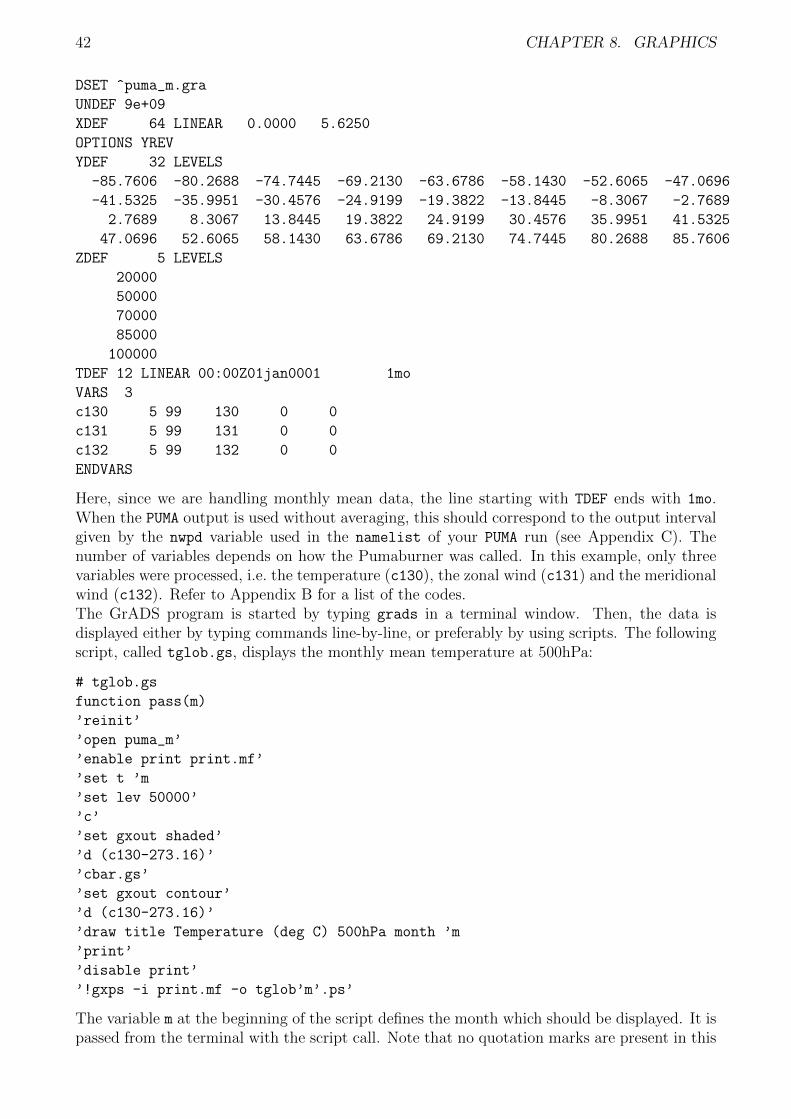
If you chose to compile it yourself, please read the comments in the first few lines of the programtext. Sometimes the srvctl tool has difficulty calculating an appropriate time axis from thedata headers of the data records, so you should check this. In particular the number of daysper year is concerned: GrADS may assume 365 days per year even though the data header says360 days per year. This is an example of what the puma_m.ctl should look like:

41

http://grads.iges.org/grads/grads.html

http://www.mpimet.mpg.de/fileadmin/software/cdo/

http://mi.uni-hamburg.de/puma/

42 CHAPTER 8. GRAPHICS

DSET ^puma_m.gra

UNDEF 9e+09

XDEF 64 LINEAR 0.0000 5.6250

OPTIONS YREV

YDEF 32 LEVELS

-85.7606 -80.2688 -74.7445 -69.2130 -63.6786 -58.1430 -52.6065 -47.0696

-41.5325 -35.9951 -30.4576 -24.9199 -19.3822 -13.8445 -8.3067 -2.7689

2.7689 8.3067 13.8445 19.3822 24.9199 30.4576 35.9951 41.5325

47.0696 52.6065 58.1430 63.6786 69.2130 74.7445 80.2688 85.7606

ZDEF 5 LEVELS

20000

50000

70000

85000

100000

TDEF 12 LINEAR 00:00Z01jan0001 1mo

VARS 3

c130 5 99 130 0 0

c131 5 99 131 0 0

c132 5 99 132 0 0

ENDVARS

Here, since we are handling monthly mean data, the line starting with TDEF ends with 1mo.When the PUMA output is used without averaging, this should correspond to the output intervalgiven by the nwpd variable used in the namelist of your PUMA run (see Appendix C). Thenumber of variables depends on how the Pumaburner was called. In this example, only threevariables were processed, i.e. the temperature (c130), the zonal wind (c131) and the meridionalwind (c132). Refer to Appendix B for a list of the codes.The GrADS program is started by typing grads in a terminal window. Then, the data isdisplayed either by typing commands line-by-line, or preferably by using scripts. The followingscript, called tglob.gs, displays the monthly mean temperature at 500hPa:

# tglob.gs

function pass(m)

’reinit’

’open puma_m’

’enable print print.mf’

’set t ’m

’set lev 50000’

’c’

’set gxout shaded’

’d (c130-273.16)’

’cbar.gs’

’set gxout contour’

’d (c130-273.16)’

’draw title Temperature (deg C) 500hPa month ’m

’print’

’disable print’

’!gxps -i print.mf -o tglob’m’.ps’

The variable m at the beginning of the script defines the month which should be displayed. It ispassed from the terminal with the script call. Note that no quotation marks are present in this

8.1. GRADS 43

line, since only GrADS specific commands are framed by quotation marks. Script commands,variable definitions, if-clauses, etc. are used without quotation marks. The script is executedby typing its name, without the suffix .gs, followed by the number of the month to be shown.For example, tglob 7 displays the monthly mean temperature at 500hPa in July. The resultingoutput file is called tglob7.ps.

The following script thh displays the time dependent temperature (in 1000hPa) of Hamburg.Here, two variables are passed to GrADS to plot, the first day and the last day. (Note that here,the file puma.gra is opened, which contains data on a daily basis). The call thh 91 180 displaysthe temperature in 1000hPa of Hamburg for the spring season from April 1st to June 30th.

# thh.gs

function pass(d1 d2)

’reinit’

’open puma’


’set lat 53’

’set lon 10’

’set lev 100000’

’set t ’d1’ ’d2

’c’

’d (c130-273.16)’

’draw title Temperature (deg C) 1000hPa in Hamburg’

’print’

’disable print’

’!gxps -i print.mf -o thh.ps’

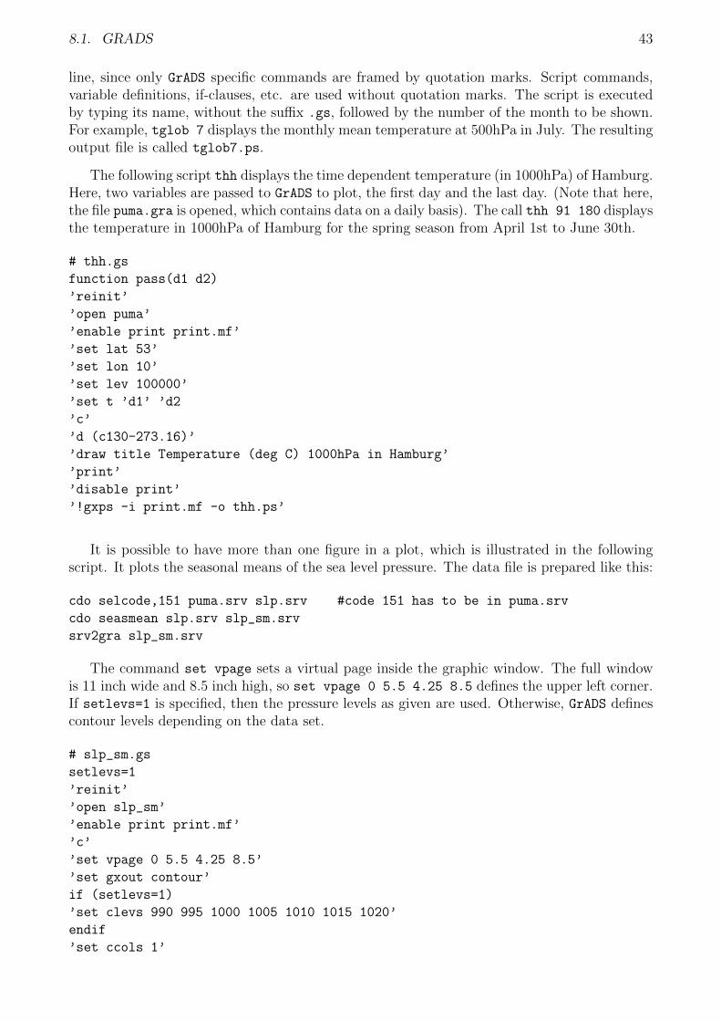
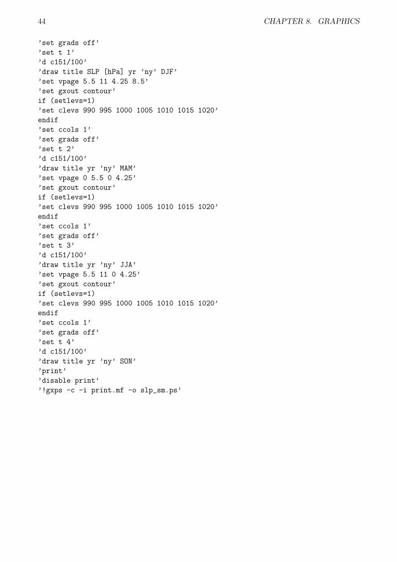
It is possible to have more than one figure in a plot, which is illustrated in the followingscript. It plots the seasonal means of the sea level pressure. The data file is prepared like this:

cdo selcode,151 puma.srv slp.srv #code 151 has to be in puma.srv

cdo seasmean slp.srv slp_sm.srv

srv2gra slp_sm.srv

The command set vpage sets a virtual page inside the graphic window. The full windowis 11 inch wide and 8.5 inch high, so set vpage 0 5.5 4.25 8.5 defines the upper left corner.If setlevs=1 is specified, then the pressure levels as given are used. Otherwise, GrADS definescontour levels depending on the data set.

# slp_sm.gs

setlevs=1

’reinit’

’open slp_sm’


’c’

’set vpage 0 5.5 4.25 8.5’


if (setlevs=1)

’set clevs 990 995 1000 1005 1010 1015 1020’

endif

’set ccols 1’

44 CHAPTER 8. GRAPHICS

’set grads off’

’set t 1’

’d c151/100’

’draw title SLP [hPa] yr ’ny’ DJF’

’set vpage 5.5 11 4.25 8.5’


if (setlevs=1)

’set clevs 990 995 1000 1005 1010 1015 1020’

endif

’set ccols 1’

’set grads off’

’set t 2’

’d c151/100’

’draw title yr ’ny’ MAM’

’set vpage 0 5.5 0 4.25’


if (setlevs=1)

’set clevs 990 995 1000 1005 1010 1015 1020’

endif

’set ccols 1’

’set grads off’

’set t 3’

’d c151/100’

’draw title yr ’ny’ JJA’

’set vpage 5.5 11 0 4.25’


if (setlevs=1)

’set clevs 990 995 1000 1005 1010 1015 1020’

endif

’set ccols 1’

’set grads off’

’set t 4’

’d c151/100’

’draw title yr ’ny’ SON’

’print’

’disable print’

’!gxps -c -i print.mf -o slp_sm.ps’

Chapter 9

Model Dynamics

9.1 Model equations and numerics

The core of the model is a set of primitive equations. They describe the conservation ofmomentum, mass, and thermal energy. Using spherical coordinates and the sigma system andwith the aid of the equation of state they can be written in the dimensionless form as follows:

Conservation of momentum:Vorticity equation

∂(ζ + f)

∂t=

1

(1− µ2)

∂Fv∂λ− ∂Fu

∂µ+ Pζ (9.1)

Divergence equation

∂D

∂t=

1

(1− µ2)

∂Fu∂λ

+∂Fv∂µ−∇2

(U2 + V 2

2(1− µ2)+ Φ + T0 ln ps

)+ PD (9.2)

Hydrostatic approximation∂Φ

∂ lnσ= −T (9.3)

Conservation of mass:Continuity equation

∂ ln ps∂t

= −1∫

0

Adσ (9.4)

Conservation of energy:First law of thermodynamics

∂T ′

∂t= − 1

(1− µ2)

∂(UT ′)

∂λ− ∂(V T ′)

∂µ+DT ′ − σ ∂T

∂σ+ κ

T

pω +

J

cp+ PT , (9.5)

with:

Fu = V (ζ + f)− σ ∂U∂σ− T ′∂ ln ps

∂λ

Fv = −U(ζ + f)− σ ∂V∂σ− T ′(1− µ2)

∂ ln ps∂µ

A = D + ~V · ∇ ln ps

and U = u cosφ, V = v cosφ.Where the variables denote:

45

46 CHAPTER 9. MODEL DYNAMICS

T temperatureT0 reference temperatureT ′ = T − T0 temperature deviation from T0ζ relative vorticityD divergenceps surface pressurep pressureΦ geopotentialt timeλ, φ longitude, latitudeµ = sinφσ = p/ps sigma vertical coordinateσ = dσ/dt vertical velocity in σ-systemω = dp/dt vertical velocity in p-systemu, v zonal, meridional component of horizontal velocity~V horizontal velocity with components U , Vf Coriolis parameterJ diabatic heating ratecp specific heat of dry air at constant pressureκ adiabatic coefficient

The set of differential equations consists of the four prognostic equations (9.1), (9.2), (9.4),and (9.5). Vorticity ζ and divergence D are scaled by the angular velocity of the earth Ω,pressures p and ps are scaled by the global mean surface pressure Ps = 1011hPa, temperaturesT and T0 are scaled by a2Ω2/R, geopotential Φ is scaled by a2Ω2/g, and time t is scaledby Ω−1,where a is the radius of the earth, R is the gas constant of dry air, and g is the gravitationalacceleration. For the parameterizations Pζ , PD and PT see section 9.2. The model can be runwith or without orography.

The horizontal representation of any model variable is given by a series of spherical har-monics. If Q is an arbitrary model variable, then its spectral representation has the form:

Q(λ, µ, t) =∑γ

Qγ(t)Yγ(λ, µ). (9.6)

Here, Yγ are the spherical harmonics, and Qγ the corresponding complex amplitudes, where γ =(n,m) designates the spectral modes (n = 1, 2, 3, . . .: total wave number; m = 0, ±1, ±2, ±3, . . .:zonal wave number), with |m| ≤ n [Holton, 1992]. The latter condition follows from the tri-angular truncation in wave number space. The truncation is done at the total wave numbernT , which can be set to nT = 21, 31, 42, 85, 127, 170, i.e. the model can be used with theT21,. . . ,T170 spectral resolution. The vertical resolution is given by nL equidistant σ-levelswith the standard value nL = 5. At the upper (σ = 0) and lower boundary (σ = 1) of themodel domain the vertical velocity is set to zero (σ = 0).

The linear contributions to the tendencies are calculated in the spectral domain, the non-linear contributions in grid point space. Therefore, at every time step, the necessary modelvariables are transformed from spectral to grid point representation by Legendre and FastFourier (FFT) transformations, and then the calculated tendencies are transformed back intothe spectral domain where the time step is carried out [for the transform method see Orszag,1970, Eliasen et al., 1970]. Because of the semi-implicit time integration scheme [Hoskins andSimmons, 1975, Simmons, Hoskins, and Burridge, 1978] the terms due to gravity wave propa-gation are integrated in time implicitly, and the remaining terms are integrated explicitly, thelatter with a leap-frog time step. In the standard model, a time step of one hour is used. A

9.2. PARAMETERIZATIONS 47

Robert-Asselin time filter [Haltiner and Williams, 1982] is applied to avoid decoupling of thetwo leap-frog time levels. The contributions to the tendencies due to vertical advection arecalculated by an energy and angular-momentum conserving vertical finite-difference scheme[Simmons and Burridge, 1981].

9.2 Parameterizations

9.2.1 Friction

The dissipative processes in the atmosphere are parameterized using a linear approach (Rayleighfriction), which describes the effects of surface drag and vertical transport of the horizontalmomentum due to small scale turbulence in the boundary layer. To achieve this, vorticity ζand divergence D are damped towards the state of rest (ζ = 0, D = 0) with the time scale τF .

The parameterization terms Pζ and PD appear in the model equations (9.1) resp. (9.2) andhave the form:

Pζ =ζ

τF+Hζ (9.7)

PD =D

τF+HD. (9.8)

The time scale (τF )l depends on the σ-level l (l = 1, . . . , nl). Usually, for the upper levels(l = 1, . . . , nl − 1) it is set to (τF )l =∞ (no friction) and for the lowest level (l = nl) a typicalvalue is (τF )l = 1 d. An explanation of the hyperdiffusion terms Hζ and HD follows in section9.2.3.

9.2.2 Diabatic heating

All the diabatic processes considered in the model are also parameterized using a linear approach(Newtonian cooling). They include the diabatic heating due to absorption and emission ofshort and long wave radiation, as well as latent and sensible heat fluxes (convection). Thetemperature T relaxes towards the restoration temperature TR with the time scale τR. Theparameterization term in the thermal energy equation (9.5) is given by:

J

cp+ PT =

TR − TτR

+HT . (9.9)

For the hyperdiffusion HT see section 9.2.3. τR depends on the σ-level l, TR on the latitude φand on the vertical coordinate σ. The restoration temperature field has the form:

TR(φ, σ) = TR(σ) + f(σ)TR(φ). (9.10)

The vertical profile is described by:

TR(σ) = (TR)tp +

√[L

2

(ztp − z(σ)

)]2+ S2 +

L

2

(ztp − z(σ)

), (9.11)

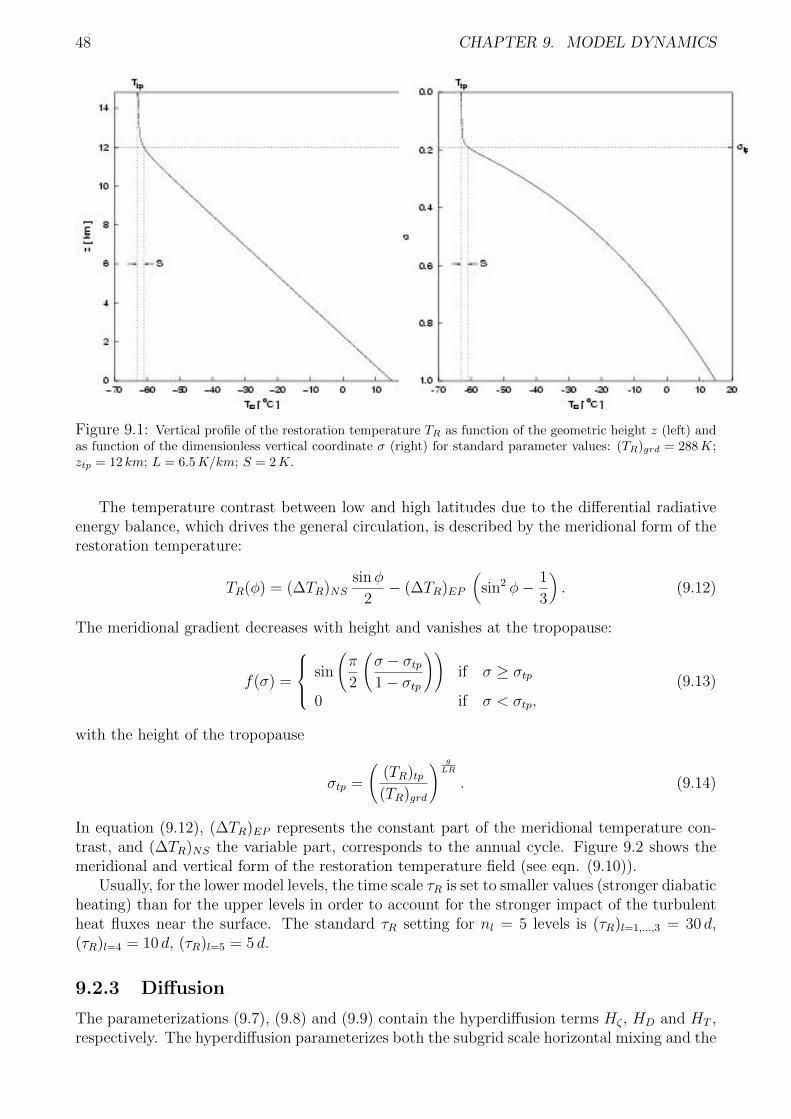
with (TR)tp = (TR)grd−Lztp. Here, z denotes the geometric height, ztp the global constant heightof the tropopause, L = −(∂TR)/(∂z) the vertical restoration temperature gradient, (TR)grd and(TR)tp the restoration temperature at the surface and at the global isothermal tropopause,respectively. S provides a smoothing of the profile at the tropopause. z(σ) is determined byan iterative method. The profile is determined by setting the parameters (TR)grd, ztp, L and S.Figure 9.1 shows the vertical profile for the standard parameter values.


Figure 9.1: Vertical profile of the restoration temperature TR as function of the geometric height z (left) andas function of the dimensionless vertical coordinate σ (right) for standard parameter values: (TR)grd = 288K;ztp = 12 km; L = 6.5K/km; S = 2K.

The temperature contrast between low and high latitudes due to the differential radiativeenergy balance, which drives the general circulation, is described by the meridional form of therestoration temperature:

TR(φ) = (∆TR)NSsinφ

2− (∆TR)EP

(sin2 φ− 1

3

). (9.12)

The meridional gradient decreases with height and vanishes at the tropopause:

f(σ) =

sin

(π

2

(σ − σtp1− σtp

))if σ ≥ σtp

0 if σ < σtp,(9.13)

with the height of the tropopause

σtp =

((TR)tp(TR)grd

) gLR

. (9.14)

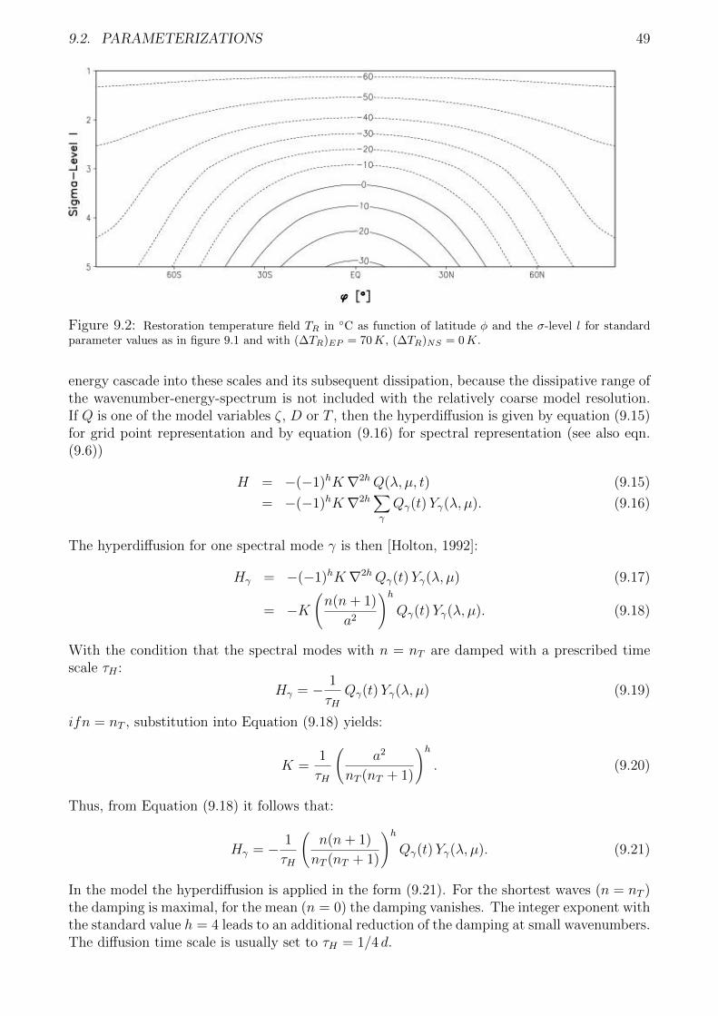
In equation (9.12), (∆TR)EP represents the constant part of the meridional temperature con-trast, and (∆TR)NS the variable part, corresponds to the annual cycle. Figure 9.2 shows themeridional and vertical form of the restoration temperature field (see eqn. (9.10)).

Usually, for the lower model levels, the time scale τR is set to smaller values (stronger diabaticheating) than for the upper levels in order to account for the stronger impact of the turbulentheat fluxes near the surface. The standard τR setting for nl = 5 levels is (τR)l=1,...,3 = 30 d,(τR)l=4 = 10 d, (τR)l=5 = 5 d.

9.2.3 Diffusion

The parameterizations (9.7), (9.8) and (9.9) contain the hyperdiffusion terms Hζ , HD and HT ,respectively. The hyperdiffusion parameterizes both the subgrid scale horizontal mixing and the

9.2. PARAMETERIZATIONS 49

Figure 9.2: Restoration temperature field TR in C as function of latitude φ and the σ-level l for standardparameter values as in figure 9.1 and with (∆TR)EP = 70K, (∆TR)NS = 0K.

energy cascade into these scales and its subsequent dissipation, because the dissipative range ofthe wavenumber-energy-spectrum is not included with the relatively coarse model resolution.If Q is one of the model variables ζ, D or T , then the hyperdiffusion is given by equation (9.15)for grid point representation and by equation (9.16) for spectral representation (see also eqn.(9.6))

H = −(−1)hK∇2hQ(λ, µ, t) (9.15)

= −(−1)hK∇2h∑γ

Qγ(t)Yγ(λ, µ). (9.16)

The hyperdiffusion for one spectral mode γ is then [Holton, 1992]:

Hγ = −(−1)hK∇2hQγ(t)Yγ(λ, µ) (9.17)

= −K(n(n+ 1)

a2

)hQγ(t)Yγ(λ, µ). (9.18)

With the condition that the spectral modes with n = nT are damped with a prescribed timescale τH :

Hγ = − 1

τHQγ(t)Yγ(λ, µ) (9.19)

ifn = nT , substitution into Equation (9.18) yields:

K =1

τH

(a2

nT (nT + 1)

)h. (9.20)

Thus, from Equation (9.18) it follows that:

Hγ = − 1

τH

(n(n+ 1)

nT (nT + 1)

)hQγ(t)Yγ(λ, µ). (9.21)

In the model the hyperdiffusion is applied in the form (9.21). For the shortest waves (n = nT )the damping is maximal, for the mean (n = 0) the damping vanishes. The integer exponent withthe standard value h = 4 leads to an additional reduction of the damping at small wavenumbers.The diffusion time scale is usually set to τH = 1/4 d.


9.3 Scaling of Variables

The variables are rendered dimensionless using the following characteristic scales:

Variable Scale Scale description

Divergence Ω Ω = angular velocityVorticity Ω Ω = angular velocityTemperature (a2Ω2)/R a = planet radius, R = gas constantPressure 101100 Pa PSURF = mean sea level pressureOrography (a2Ω2)/g g = gravity

9.4 Vertical Discretization

ζ,D, T ′

ζ,D, T ′

ζ,D, T ′

ζ,D, T ′

ζ,D, T ′

σ

σ

σ

σ

p = ps, σ = 0

p = 0, σ = 0

Level σ V ariables

1.0

0.9

0.8

0.7

0.6

0.5

0.4

0.3

0.2

0.1

0.0

5.5

5

4.5

4

3.5

3

2.5

2

1.5

1

0.5

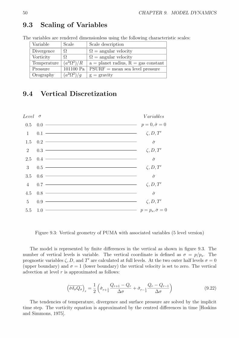
Figure 9.3: Vertical geometry of PUMA with associated variables (5 level version)

The model is represented by finite differences in the vertical as shown in figure 9.3. Thenumber of vertical levels is variable. The vertical coordinate is defined as σ = p/ps. Theprognostic variables ζ,D, and T ′ are calculated at full levels. At the two outer half levels σ = 0(upper boundary) and σ = 1 (lower boundary) the vertical velocity is set to zero. The verticaladvection at level r is approximated as follows:

(σδσQσ

)r

=1

2

(σr+ 1

2

Qr+1 −Qr

∆σ+ σr− 1

2

Qr −Qr−1

∆σ

)(9.22)

The tendencies of temperature, divergence and surface pressure are solved by the implicittime step. The vorticity equation is approximated by the centred differences in time [Hoskinsand Simmons, 1975].

9.5. PUMA FLOW DIAGRAM 51

9.5 PUMA Flow Diagram

The diagram 9.4 shows the route through the main program PUMA, with the names of themost important subroutines.

PUMA is the main program. It calls the three subroutines Prolog, Master and Epilog . Prologdoes all initialization. It calls the following subroutines: gauaw computes gaussian abscissasand weights. inilat initializes some utility arrays like square of cosine of latitude etc. legpriprints the arrays of gauaw and inilat. readnl reads the namelist from standard input. initpminitializes most vertical arrays and some in the spectral domain. initsi computes arrays for thesemi-implicit scheme. legini computes all polynomials needed for the Legendre transformation.restart starts the model from the restart file, if selected of a previous run. initfd initializesspectral arrays. setzt sets up the restoration temperature array. noise puts a selectable form ofnoise into lnPs. setztex is a special version of setzt for dipole experiments.

Master does some initial timesteps on initial runs, then it runs the time loop for the selectedintegration time. It calls the following subroutines: makebm constructs the array bm, gridpointdoes all transformations and calculations in the grid point domain. sp2fc converts spectral toFourier coefficients (inverse Legendre transf.), dv2uv divergence and vorticity to u and v (impliesspectral to Fourier), fc2gp Fourier coefficients to grid points (fast Fourier transformation),calcgp calculations in grid point space, gp2fc grid points to Fourier coefficients (fast Fouriertransformation), fc2sp Fourier coefficients to spectral (direct Legendre transf.), mktend makestendencies (implies Fourier to spectral), spectral does all calculations in the spectral domain,outsp writes spectral fields in physical dimensions on an output file, and diag writes selectedfields and parameters to the standard output. Epilog writes the restart file.

9.6 Initialization

The model starts either from a restart file or with the atmosphere at rest. The defaults makethe initial state a motionless, stable stratified atmosphere. For an initial start the divergenceand the relative vorticity are set to zero (only mode(1,0) of vorticity is set to the planetaryvorticity). The temperature is initialized as a constant horizontal field. The vertical distributionis adopted from the restoration temperature, usually a stable stratification. The initializationof the logarithm of the surface pressure is controlled by the namelist variable kick: kick=0sets all modes to zero, so the model runs with constant zones without eddies, kick=1 generatesrandom white noise and kick=2 generates random white noise that is symmetrical about theequator. Runs started with kick=1 or 2 are irreproducible due to the randomization. Forreproducible runs with eddies use kick=3 which only initializes mode(1,2) of lnPs with a smallconstant. The amplitude of the noise perturbation is normalized to 0.1 hPa (1.e-4 of the meansurface pressure).

A radiative equilibrium temperature field for the run is set up by setzt: First, a global meanradiative equilibrium temperature profile TR(σ) is defined. A hyperbolic function of height isused to provide TR(σ), as illustrated in Figure 9.1. With z → − ∞ the profile tends to auniform lapse rate, alr, passing through the temperature tgr at z = 0. With z → +∞ theprofile becomes isothermal. The transition takes place at the height ztrop. The sharpnessof the tropopause is controlled by the parameter dttrp. When dttrp = 0,the lapse ratechanges discontinuously at ztrop. For dttrp small but positive, the transition is spread. Thehydrostatic relation is used to determine the heights and hence the temperatures of the modellevels.


9.7 Computations in spectral domain

The subroutinespectral performs one timestep. Details of the time stepping scheme are givenin [Hoskins and Simmons, 1975]. The adiabatic tendencies (advection, etc.) are used. Thenormal time step is centered in time, and includes a Robert time filter to control time splitting.For the first nkits time steps, short initial time steps, an initial forward timestep followed by acentred step, each twice its predecessor, are taken in order to initiate a run from data at onlyone time level. No Robert filter is included in the short steps. The subroutine calculates thespectral tendencies due to Newtonian cooling, Rayleigh friction and hyperdiffusion:

9.7. COMPUTATIONS IN SPECTRAL DOMAIN 53

puma Main program

? mpstart Multi processing startup

? prolog Call initialization routines

? master Perform time loop for NRUN time steps

? gridpoint Call transformation and grid point routines

? sp2fc Inverse Legendre transformation

? dv2uv Divergence and vorticity to u,v - wind components

? fc2gp Fourier coefficients to grid points (Inverse FFT)

? calcgp Calculations in grid point space

? gp2fc Grid point to Fourier coefficients (FFT)

? mktend Make tendencies for spectral domain

? mpsumsc MP sum and scatter

? outsp Write prognostic fields to file (puma data)

? diag Write diagnostics to standard output

? spectral Perform spectral calculations and time stepping

time loop

-

epilog Write restart file (puma status)

? mpstop MP terminate (end all processes)

Figure 9.4: Flow diagram of main routines

Chapter 10

Preprocessor

In many cases the setup of PUMA experiments can be defined using namelist variables eithervia MoSt or with editing the namelist file. In these cases PUMA can run without any startupfiles containing boundary conditions.

For more complex experiments, like changes in orography or ground temperature, predefinedvertical and horizontal gradients of the restoration temperature field and more, it is necessaryto create files for boundary conditions.

This is done with the PPP (short for Puma Pre-Processor).The PPP is a stand alone program, that can be called inside the modelstarter MoSt or

explicitely by the user. It shares the namelist file puma namelist with PUMA, because bothprograms must use the same parameters for consistency.

The use in MoSt is currently restricted for using an orography in PUMA. If the orographyoption is checked in MoSt the PPP will be run before creating the run time environment forthe model. The PPP creates startup definitions for orography, constant and time variable partof the restoration temperature and an initial field for surface pressure.

Additionally the simple orography modifier of MoSt may be used to rise or lower parts ofthe orography. A mouseclick on the button Preprocess will then call the PPP and make allnecessary adjustions to start fields.More complex setups must be performed by either using some of the PPP namelist parameters orby adding code to PPP itself. This requires however a good knowledge of the FORTRAN-90 pro-gramming language and of the model interna. The source code is in the file Most16/puma/src/ppp.f90.To make changes easier the PPP has two subroutines named modify orography and mod-ify ground temperature. These are the recommended places to add user code.

More details can be found in the FORTRAN-90 code of the PPP itself.

55

56 CHAPTER 10. PREPROCESSOR

Chapter 11

Benchmark

11.1 Performance

PUMA on XEON server

57

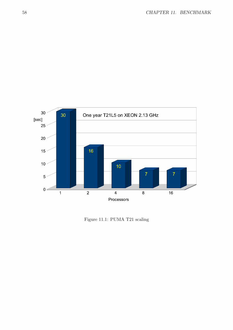
58 CHAPTER 11. BENCHMARK

Figure 11.1: PUMA T21 scaling

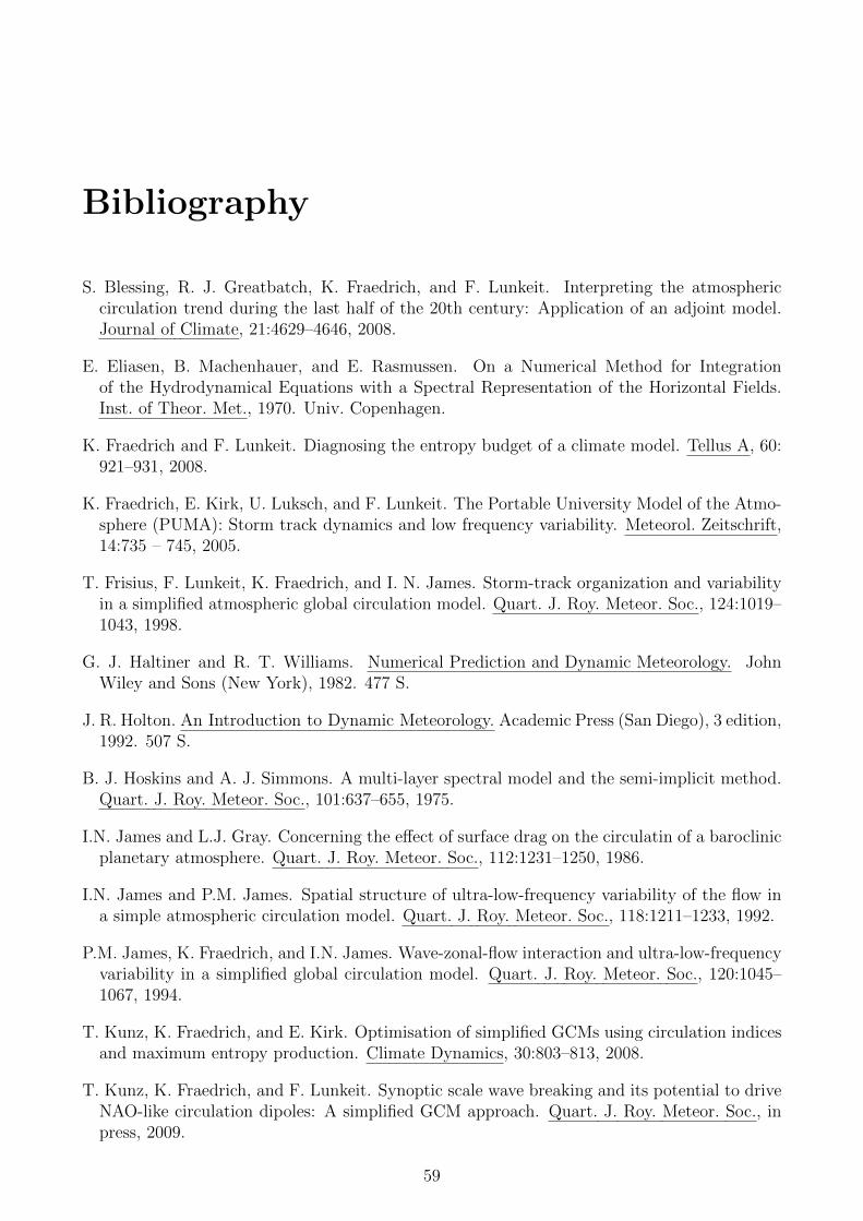
Bibliography

S. Blessing, R. J. Greatbatch, K. Fraedrich, and F. Lunkeit. Interpreting the atmosphericcirculation trend during the last half of the 20th century: Application of an adjoint model.Journal of Climate, 21:4629–4646, 2008.

E. Eliasen, B. Machenhauer, and E. Rasmussen. On a Numerical Method for Integrationof the Hydrodynamical Equations with a Spectral Representation of the Horizontal Fields.Inst. of Theor. Met., 1970. Univ. Copenhagen.

K. Fraedrich and F. Lunkeit. Diagnosing the entropy budget of a climate model. Tellus A, 60:921–931, 2008.

K. Fraedrich, E. Kirk, U. Luksch, and F. Lunkeit. The Portable University Model of the Atmo-sphere (PUMA): Storm track dynamics and low frequency variability. Meteorol. Zeitschrift,14:735 – 745, 2005.

T. Frisius, F. Lunkeit, K. Fraedrich, and I. N. James. Storm-track organization and variabilityin a simplified atmospheric global circulation model. Quart. J. Roy. Meteor. Soc., 124:1019–1043, 1998.

G. J. Haltiner and R. T. Williams. Numerical Prediction and Dynamic Meteorology. JohnWiley and Sons (New York), 1982. 477 S.

J. R. Holton. An Introduction to Dynamic Meteorology. Academic Press (San Diego), 3 edition,1992. 507 S.

B. J. Hoskins and A. J. Simmons. A multi-layer spectral model and the semi-implicit method.Quart. J. Roy. Meteor. Soc., 101:637–655, 1975.

I.N. James and L.J. Gray. Concerning the effect of surface drag on the circulatin of a baroclinicplanetary atmosphere. Quart. J. Roy. Meteor. Soc., 112:1231–1250, 1986.

I.N. James and P.M. James. Spatial structure of ultra-low-frequency variability of the flow ina simple atmospheric circulation model. Quart. J. Roy. Meteor. Soc., 118:1211–1233, 1992.

P.M. James, K. Fraedrich, and I.N. James. Wave-zonal-flow interaction and ultra-low-frequencyvariability in a simplified global circulation model. Quart. J. Roy. Meteor. Soc., 120:1045–1067, 1994.

T. Kunz, K. Fraedrich, and E. Kirk. Optimisation of simplified GCMs using circulation indicesand maximum entropy production. Climate Dynamics, 30:803–813, 2008.

T. Kunz, K. Fraedrich, and F. Lunkeit. Synoptic scale wave breaking and its potential to driveNAO-like circulation dipoles: A simplified GCM approach. Quart. J. Roy. Meteor. Soc., inpress, 2009.

59

60 BIBLIOGRAPHY

F. Lunkeit, K. Fraedrich, and S.E. Bauer. Storm tracks in a warmer climate: Sensitivity studieswith a simplified global circulation model. Climate Dynamics, 14:813–826, 1998.

N. Mole and I.N. James. Baroclinic adjustment in a zonally varying flow. Quart. J. Roy.Meteor. Soc., 116:247–268, 1990.

S. A. Orszag. Transform Method for the Calculation of Vector-Coupled Sums: Application tothe Spectral Form of the Vorticity Equation. J. Atmos. Sci., 27:890–895, 1970.

V. Perez-Munuzuri, R. Deza, K. Fraedrich, T. Kunz, and F. Lunkeit. Coherence resonance inan atmospheric global circulation model. Phys. Rev. E, 71:065602(1–4), 2005.

A. J. Simmons and D. Burridge. An Energy and Angular-Momentum Conserving VerticalFinite-Difference Scheme and Hybrid Vertical Coordinates. Mon. Wea. Rev., 109:758–766,1981.

A. J. Simmons, B. J. Hoskins, and D. M. Burridge. Stability of the Semi-Implicit Method ofTime Integration. Mon. Wea. Rev., 106:405–412, 1978.

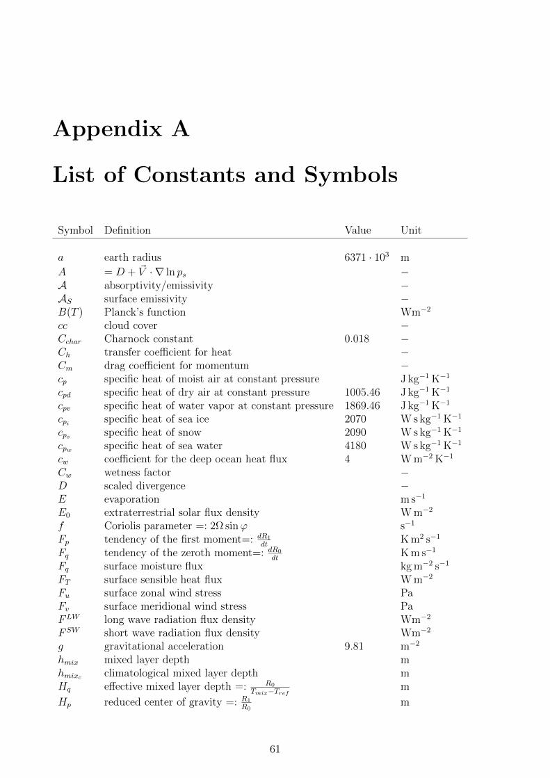
Appendix A

List of Constants and Symbols

Symbol Definition Value Unit

a earth radius 6371 · 103 m

A = D + ~V · ∇ ln ps −A absorptivity/emissivity −AS surface emissivity −B(T ) Planck’s function Wm−2

cc cloud cover −Cchar Charnock constant 0.018 −Ch transfer coefficient for heat −Cm drag coefficient for momentum −cp specific heat of moist air at constant pressure J kg−1 K−1

cpd specific heat of dry air at constant pressure 1005.46 J kg−1 K−1

cpv specific heat of water vapor at constant pressure 1869.46 J kg−1 K−1

cpi specific heat of sea ice 2070 W s kg−1 K−1

cps specific heat of snow 2090 W s kg−1 K−1

cpw specific heat of sea water 4180 W s kg−1 K−1

cw coefficient for the deep ocean heat flux 4 W m−2 K−1

Cw wetness factor −D scaled divergence −E evaporation m s−1

E0 extraterrestrial solar flux density W m−2

f Coriolis parameter =: 2Ω sinϕ s−1

Fp tendency of the first moment=: dR1

dtK m2 s−1

Fq tendency of the zeroth moment=: dR0

dtK m s−1

Fq surface moisture flux kg m−2 s−1

FT surface sensible heat flux W m−2

Fu surface zonal wind stress PaFv surface meridional wind stress PaFLW long wave radiation flux density Wm−2

F SW short wave radiation flux density Wm−2

g gravitational acceleration 9.81 m−2

hmix mixed layer depth mhmixc climatological mixed layer depth mHq effective mixed layer depth =: R0

Tmix−Trefm

Hp reduced center of gravity =: R1

R0m

61

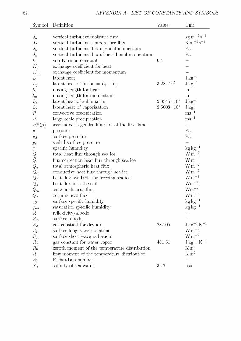
62 APPENDIX A. LIST OF CONSTANTS AND SYMBOLS


Jq vertical turbulent moisture flux kg m−2 s−1

JT vertical turbulent temperature flux K m−2 s−1

Ju vertical turbulent flux of zonal momentum PaJv vertical turbulent flux of meridional momentum Pak von Karman constant 0.4 −Kh exchange coefficient for heat −Km exchange coefficient for momentum −L latent heat J kg−1

Lf latent heat of fusion = Ls − Lv 3.28 · 105 J kg−1

lh mixing length for heat mlm mixing length for momentum mLs latent heat of sublimation 2.8345 · 106 J kg−1

Lv latent heat of vaporization 2.5008 · 106 J kg−1

Pc convective precipitation ms−1

Pl large scale precipitation ms−1

Pmn (µ) associated Legendre function of the first kind −p pressure PapS surface pressure Paps scaled surface pressure −q specific humidity kg kg−1

Q total heat flux through sea ice W m−2

Q flux correction heat flux through sea ice W m−2

Qa total atmospheric heat flux W m−2

Qc conductive heat flux through sea ice W m−2

Qf heat flux available for freezing sea ice W m−2

Qg heat flux into the soil Wm−2

Qm snow melt heat flux Wm−2

Qo oceanic heat flux W m−2

qS surface specific humidity kg kg−1

qsat saturation specific humidity kg kg−1

R reflexivity/albedo −RS surface albedo −Rd gas constant for dry air 287.05 J kg−1 K−1

Rl surface long wave radiation W m−2

Rs surface short wave radiation W m−2

Rv gas constant for water vapor 461.51 J kg−1 K−1

R0 zeroth moment of the temperature distribution K mR1 first moment of the temperature distribution K m2

Ri Richardson number −Sw salinity of sea water 34.7 psu

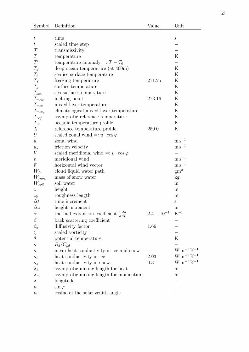
63


t time st scaled time step −T transmissivity −T temperature KT ′ temperature anomaly =: T − T0 −Td deep ocean temperature (at 400m) KTi sea ice surface temperature KTf freezing temperature 271.25 KTs surface temperature KTsea sea surface temperature KTmelt melting point 273.16 KTmix mixed layer temperature KTmixc climatological mixed layer temperature KTref asymptotic reference temperature KTw oceanic temperature profile KT0 reference temperature profile 250.0 KU scaled zonal wind =: u · cosϕ −u zonal wind m s−1

u∗ friction velocity m s−1

V scaled meridional wind =: v · cosϕ −v meridional wind m s−1

~v horizontal wind vector m s−1

WL cloud liquid water path gm2

Wsnow mass of snow water kgWsoil soil water mz height mz0 roughness length m∆t time increment s∆z height increment m

α thermal expansion coefficient 1ρdρdT

2.41 · 10−4 K−1

β back scattering coefficient −βd diffusivity factor 1.66 −ζ scaled vorticity −θ potential temperature Kκ Rd/Cpd −κ mean heat conductivity in ice and snow W m−1 K−1

κi heat conductivity in ice 2.03 W m−1 K−1

κs heat conductivity in snow 0.31 W m−1 K−1

λh asymptotic mixing length for heat mλm asymptotic mixing length for momentum mλ longitude −µ sinϕ −µ0 cosine of the solar zenith angle −

64 APPENDIX A. LIST OF CONSTANTS AND SYMBOLS


ρ density of air kg m−3

ρi density of sea ice 920 kg m−3

ρs density of snow 330 kg m−3

ρw density of sea water 1030 kg m−3

ρo density of fresh water 1000 kg m−3

σ normalized pressure coordinate =: p/ps −σ vertical velocity in σ system −σSB Stefan-Bolzmann constant 5.67 · 10−8 Wm−2K−4

τN cloud optical depth −τF time scale for RF −τR time scale for NC −τT time scale for temperature flux correction sτh time scale for depth flux correction sφ geopotential height := g · z m2 s−2

φ scaled geopotential height −ϕ latitude −χ scaled velocity potential −ψ scaled stream function −Ω angular velocity of the earth 7.292 · 10−5 s−1

ω0 single scattering albedo −

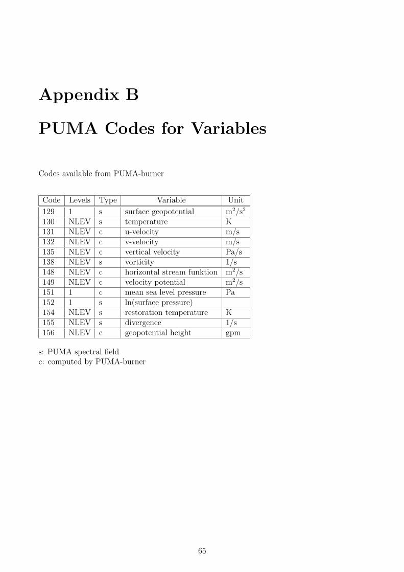
Appendix B

PUMA Codes for Variables

Codes available from PUMA-burner

Code Levels Type Variable Unit

129 1 s surface geopotential m2/s2

130 NLEV s temperature K131 NLEV c u-velocity m/s132 NLEV c v-velocity m/s135 NLEV c vertical velocity Pa/s138 NLEV s vorticity 1/s148 NLEV c horizontal stream funktion m2/s149 NLEV c velocity potential m2/s151 1 c mean sea level pressure Pa152 1 s ln(surface pressure)154 NLEV s restoration temperature K155 NLEV s divergence 1/s156 NLEV c geopotential height gpm

s: PUMA spectral fieldc: computed by PUMA-burner

65

66 APPENDIX B. PUMA CODES FOR VARIABLES

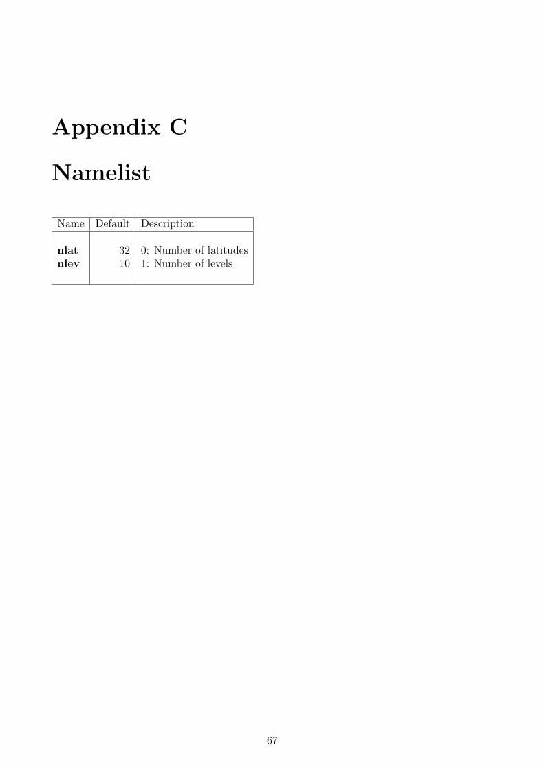
Appendix C

Namelist

Name Default Description

nlat 32 0: Number of latitudesnlev 10 1: Number of levels

67

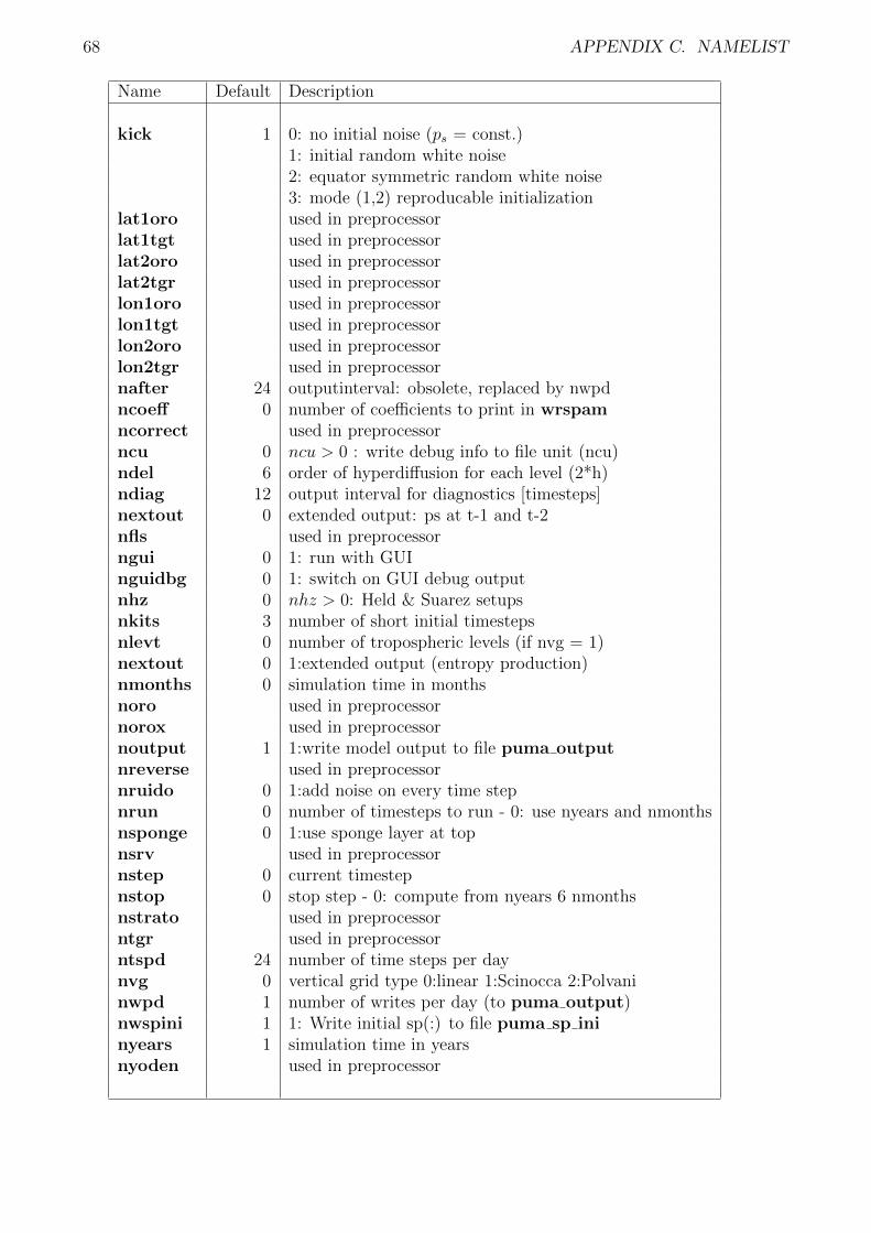
68 APPENDIX C. NAMELIST


kick 1 0: no initial noise (ps = const.)1: initial random white noise2: equator symmetric random white noise3: mode (1,2) reproducable initialization

lat1oro used in preprocessorlat1tgt used in preprocessorlat2oro used in preprocessorlat2tgr used in preprocessorlon1oro used in preprocessorlon1tgt used in preprocessorlon2oro used in preprocessorlon2tgr used in preprocessornafter 24 outputinterval: obsolete, replaced by nwpdncoeff 0 number of coefficients to print in wrspamncorrect used in preprocessorncu 0 ncu > 0 : write debug info to file unit (ncu)ndel 6 order of hyperdiffusion for each level (2*h)ndiag 12 output interval for diagnostics [timesteps]nextout 0 extended output: ps at t-1 and t-2nfls used in preprocessorngui 0 1: run with GUInguidbg 0 1: switch on GUI debug outputnhz 0 nhz > 0: Held & Suarez setupsnkits 3 number of short initial timestepsnlevt 0 number of tropospheric levels (if nvg = 1)nextout 0 1:extended output (entropy production)nmonths 0 simulation time in monthsnoro used in preprocessornorox used in preprocessornoutput 1 1:write model output to file puma outputnreverse used in preprocessornruido 0 1:add noise on every time stepnrun 0 number of timesteps to run - 0: use nyears and nmonthsnsponge 0 1:use sponge layer at topnsrv used in preprocessornstep 0 current timestepnstop 0 stop step - 0: compute from nyears 6 nmonthsnstrato used in preprocessorntgr used in preprocessorntspd 24 number of time steps per daynvg 0 vertical grid type 0:linear 1:Scinocca 2:Polvaninwpd 1 number of writes per day (to puma output)nwspini 1 1: Write initial sp(:) to file puma sp ininyears 1 simulation time in yearsnyoden used in preprocessor

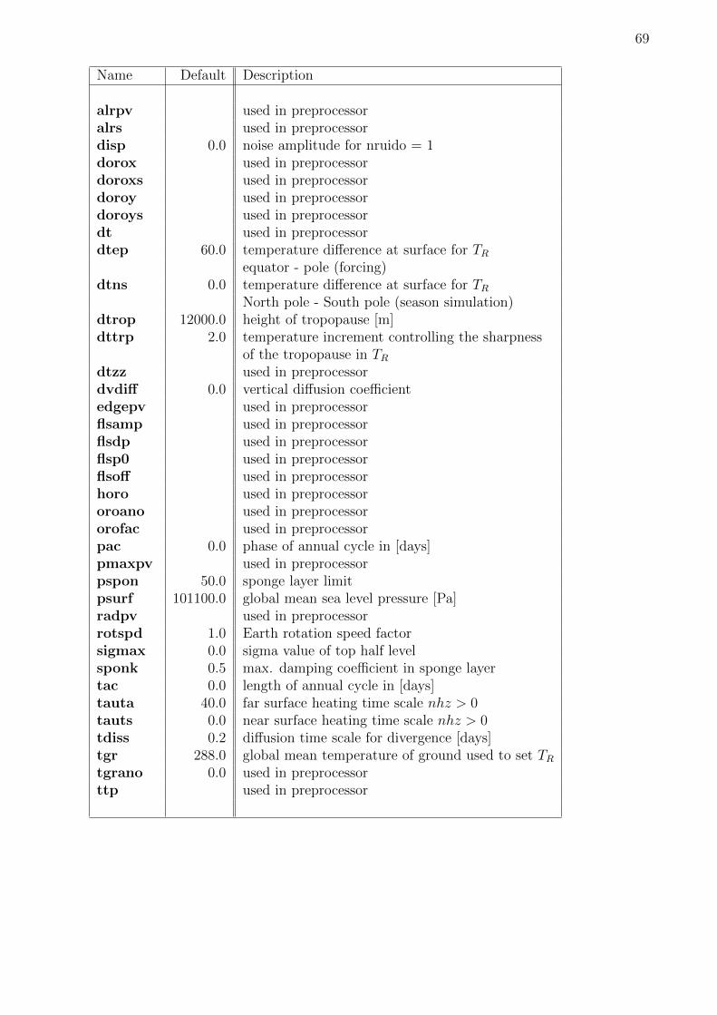
69


alrpv used in preprocessoralrs used in preprocessordisp 0.0 noise amplitude for nruido = 1dorox used in preprocessordoroxs used in preprocessordoroy used in preprocessordoroys used in preprocessordt used in preprocessordtep 60.0 temperature difference at surface for TR

equator - pole (forcing)dtns 0.0 temperature difference at surface for TR

North pole - South pole (season simulation)dtrop 12000.0 height of tropopause [m]dttrp 2.0 temperature increment controlling the sharpness

of the tropopause in TRdtzz used in preprocessordvdiff 0.0 vertical diffusion coefficientedgepv used in preprocessorflsamp used in preprocessorflsdp used in preprocessorflsp0 used in preprocessorflsoff used in preprocessorhoro used in preprocessororoano used in preprocessororofac used in preprocessorpac 0.0 phase of annual cycle in [days]pmaxpv used in preprocessorpspon 50.0 sponge layer limitpsurf 101100.0 global mean sea level pressure [Pa]radpv used in preprocessorrotspd 1.0 Earth rotation speed factorsigmax 0.0 sigma value of top half levelsponk 0.5 max. damping coefficient in sponge layertac 0.0 length of annual cycle in [days]tauta 40.0 far surface heating time scale nhz > 0tauts 0.0 near surface heating time scale nhz > 0tdiss 0.2 diffusion time scale for divergence [days]tgr 288.0 global mean temperature of ground used to set TRtgrano 0.0 used in preprocessorttp used in preprocessor

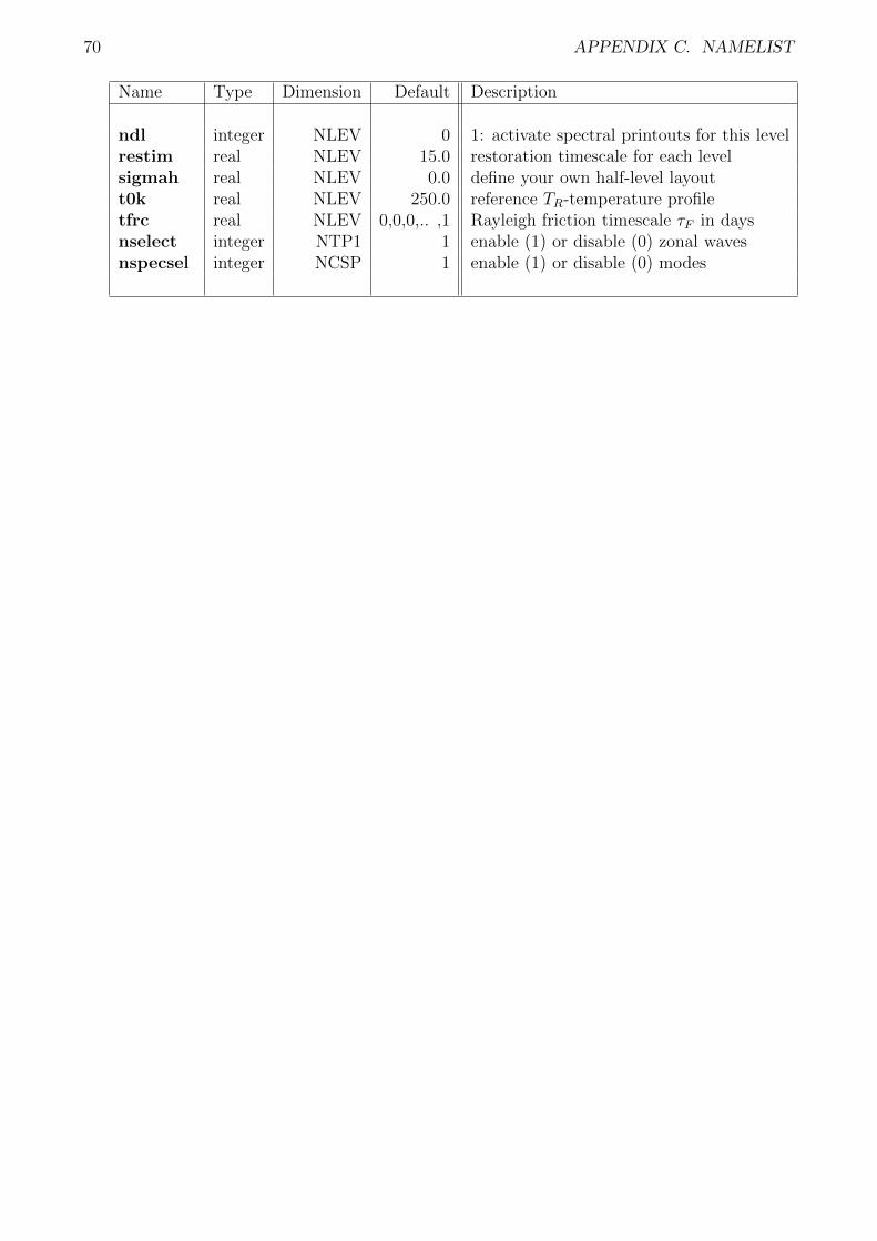
70 APPENDIX C. NAMELIST

Name Type Dimension Default Description

ndl integer NLEV 0 1: activate spectral printouts for this levelrestim real NLEV 15.0 restoration timescale for each levelsigmah real NLEV 0.0 define your own half-level layoutt0k real NLEV 250.0 reference TR-temperature profiletfrc real NLEV 0,0,0,.. ,1 Rayleigh friction timescale τF in daysnselect integer NTP1 1 enable (1) or disable (0) zonal wavesnspecsel integer NCSP 1 enable (1) or disable (0) modes

User’s Guide Version 16 - Meteorologisches Institut · PDF filePUMA User’s Guide...

Documents

Transcript of User’s Guide Version 16 - Meteorologisches Institut · PDF filePUMA User’s Guide...