
US Dairy Product Trade: Modeling Approaches and the · PDF fileprotein concentrates (MPCs) ......
152
US Dairy Product Trade: Modeling Approaches and the Impact of New Product Formulations Final Report for NRI Grant # 2001-35400-10249 by Charles F. Nicholson Cornell Program on Dairy Markets and Policy Cornell University, Ithaca, NY 14853-7801 USA and Phillip M. Bishop New Zealand Institute of Economic Research Wellington, New Zealand March 2004 Copyright 2004 by Charles F. Nicholson and Phillip M. Bishop. Readers may make verbatim copies of this document for non-commercial purposes by any means provided that this copyright notice appears on all such copies.
Transcript of US Dairy Product Trade: Modeling Approaches and the · PDF fileprotein concentrates (MPCs) ......

US Dairy Product Trade: Modeling Approaches and the Impact of New
Product Formulations
Final Report for NRI Grant # 2001-35400-10249
by
Charles F. Nicholson Cornell Program on Dairy Markets and Policy
Cornell University, Ithaca, NY 14853-7801 USA
and
Phillip M. Bishop
New Zealand Institute of Economic Research
Wellington, New Zealand
March 2004
Copyright 2004 by Charles F. Nicholson and Phillip M. Bishop. Readers may make verbatim copies of this document for non-commercial purposes by any means provided that this copyright notice appears on all such copies.

Table of Contents
Executive Summary........................................................................................ i
List of Figures ................................................................................................ v
List of Tables ................................................................................................ vi
Chapter 1: Introduction................................................................................ 1
Recent Trade Policy Changes .............................................................................2
Technological Developments in the Dairy and Food Processing Industries ................................................................................3
Review of Analytical Literature ...........................................................................4
Research Objectives..........................................................................................6
Chapter 1 References........................................................................................7
Chapter 2: Trade Liberalization and the US Dairy Industry........................10
Introduction ................................................................................................... 10
World Trade in Dairy Products ......................................................................... 10
US Dairy Product Imports and Exports, 1990-2001 ............................................ 11
Trade Liberalization and US Dairy Trade Policy, 1990-2001 ................................ 21
Impacts of Trade Liberalization on the US Dairy Industry ................................... 33
Recent Dairy Trade Issues............................................................................... 38
The Future of Dairy Trade Liberalization ........................................................... 41
Concluding Comments..................................................................................... 42
Chapter 2 References...................................................................................... 43
Chapter 3: Modeling Tariff-Rate Quotas as a Mixed Complementarity Problem ...................................................................................................45
Introduction ................................................................................................... 45
The Basics of Optimization............................................................................... 45
The Mixed Complementarity Problem................................................................ 51
Multi-Region Models........................................................................................ 52
Modeling Tariff-Rate Quotas ............................................................................ 66

Bringing It All Together ................................................................................... 68
Concluding Remarks ....................................................................................... 72
Chapter 3 References...................................................................................... 72
Chapter 4: Modeling World Dairy Product Trade with a Mixed Complementarity Problem Formulation...................................................75
Introduction ................................................................................................... 75
The Mixed Complementarity Problem Restated.................................................. 78
The World Dairy Trade Model Formulation ........................................................ 81
Data Considerations ........................................................................................ 89
Concluding Comments..................................................................................... 89
Chapter 4 References...................................................................................... 91
Chapter 5: Market Impacts of Milk Protein Concentrate Imports ..............93
Background.................................................................................................... 93
A Mixed Complementarity Model of the US Dairy Industry with Trade.................. 93
Model Data..................................................................................................... 95
Results and Discussion .................................................................................. 110
Scenarios Simulated ................................................................................ 110
Summary of Market Impacts .................................................................... 111
Conclusions and Implications ......................................................................... 112
Chapter 5 References.................................................................................... 113
Appendix: Additional Discussion of Model Structure and Equations................... 119

i
Executive Summary
Several domestic and international developments increased interest among the US dairy industry in world markets during the 1990s. One development was the passage of the NAFTA and Uruguay Round (URA) trade agreements in the mid-decade, and their successors, the current “Doha Round” of international trade negotiations now underway. Another development during the 1990s was additional (positive) experience gained by the US dairy industry in export markets. Much of this experience came about because increases in world market prices for butter and powder in 1995-96 made US exports more competitive. The Dairy Export Incentive Program (DEIP) is also credited with improving the ability of US exporters to move powders, butter and cheese into international markets.
At the same time, there has been an increased level of concern about possible negative impacts of past and potential liberalization of dairy product trade. Rapid growth in imports of products designed to circumvent US tariffs on dairy products, such as milk protein concentrates (MPCs) have caused a great deal of concern about their impacts on US farm milk prices. Viewed in larger perspective, this issue demonstrates how much the US dairy trade policy environment had changed since the early 1990s. The NAFTA had placed the US on the road to something close to free trade in dairy products with Mexico, and the URA had committed the US to reductions in domestic support and export subsidies and increases in market access for dairy products.
Importantly in light of the rapid pace of technological developments in dairy processing, these trade agreements also placed limits on the US’ ability to modify tariff schedules to address new product formulations. As a result of these diverse developments, there is continued interest in understanding the world market for dairy products, the impacts of imports on the US dairy industry and the potential for growth in US exports. The overall objectives of this report are:
1) To review recent patterns of US dairy trade and changes in trade policies affecting US trade in dairy products;
2) To develop improved analytical frameworks for empirical economic analysis of the impacts of dairy product trade and trade liberalization on the US dairy industry;
and
3) To implement an empirical model formulation to assess the impacts of imports of dairy product formulations that circumvent existing trade barriers, using milk protein concentrates (MPCs) as an example.

ii
The key findings of this study are:
• A number of new technologies for separating the components of milk (e.g., fat, protein, lactose) have become commercially viable and other similar technologies will become viable in the near future. This will increase the economic viability of transporting dairy components long distances, and will promote the formulation of new products to better meet the demands of both dairy processing companies and final consumers. This will place tremendous pressure on policies aimed at pricing milk and protecting domestic producers. (Chapter 1)
• Much of the analytical research to date fails to account for many of the important facets that determine prices, trade patterns, and competitiveness in the dairy industry today. In general, the existing models are too highly aggregated with respect to regional and product specificity, overly simplistic with respect to policy detail, and naive with respect to the technical relationships and marketing arrangements peculiar to the dairy sector. (Chapter 1)
• US dairy trade policy has undergone great change in the past decade. US participation in the NAFTA and the Uruguay Round Agreement (URA) has allowed relatively modest increases in dairy product imports, and laid the groundwork for current efforts to further liberalize agricultural trade. (Chapter 2)
• The US is a relatively small player in world dairy markets. It exported less than 4% of the volume of major commodities (butter, cheese, and milk powders) in 1999 and 2000. The European Union, New Zealand, and Australia are the world’s major dairy product exporters. (Chapter 2)
• Despite its small share of world dairy trade, the US exported nearly $900 million worth of dairy products in 2001. The value of dairy product exports has grown more rapidly than imports since 1990, with whey and whey products an important and fast-growing export. (Chapter 2)
• The value of US imports ($1.5 billion), however, was larger than the value of exports in 2000, and imports have also grown some 80% since 1990. The most important US imports are specialty cheeses and casein products. Imports of milk protein concentrates grew rapidly from 1995 to 2000. (Chapter 2)
• Despite the growth in the value of imports, imports still account for less than 3% of commercial disappearance, measured as either fat or nonfat solids. This percentage was roughly constant from 1990 to 1997, then increased in 1998 due to butter and MPC imports. (Chapter 2)
• The URA commits the US to a broader range of trade-related policies, including reductions in the overall value of “domestic support” programs—which may include the Dairy Price Support Program. However, the impacts of the URA on the US dairy industry to date are modest. (Chapter 2)

iii
• A number of studies have examined the potential impacts of trade liberalization on the US dairy industry. These studies indicate that past and future reductions in tariffs and increases in import quotas are unlikely to result in either dramatic benefits for the US dairy industry, or dramatic negative effects. Most studies predict small reductions (1-2%) in US dairy farm income when various trade barriers are reduced, as long as all major dairy exporters participate in the reductions. However, most of these studies address only short-term effects and may not capture long-term opportunities to export certain products. (Chapter 2)
• Key dairy trade issues in recent years include the increase in MPC imports, ongoing disputes with Canada about its export subsidies, the role of what are called “state trading enterprises” in dairy trade, and the impacts of provisions other than tariffs and quotas (e.g., sanitary and phytosanitary (SPS) provisions) on the prospects for dairy trade. (Chapter 2)
• The prospects for future dairy trade liberalization are uncertain. The US is keen to see further agricultural trade liberalization, but the EU and Canada are reluctant because of the potential negative impacts on their dairy farms. The US should focus attention not just on the reduction of export subsidies, but also on provisions that may be used as trade barriers, such as import licensing, SPS, and other technical barriers to trade. (Chapter 2)
• The use of tariff-rate quotas (TRQs) is widespread, especially in agricultural and other primary-sector trade policy settings. Many of the extant trade models can be reformulated as mixed complementarity problems (MCPs). They are then capable of being used to analyze complex of TRQ instruments. (Chapter 3)
• The use of a mixed complementarity problem framework has great potential to incorporate characteristics of dairy trade not yet adequately addressed by existing empirical models. These characteristics include direct modeling of ad valorem tariffs, imperfectly competitive international markets (including state trading enterprises such as the former New Zealand Dairy Board, now reincarnated as Fonterra), nonlinearities in component balance equations due to variations in raw milk component content by region, and development of new intermediate products that circumvent existing trade barriers. (Chapter 4)
• Imports of milk protein concentrates (MPC) classified under Chapter 4 of the Harmonized Tariff Schedule have modest impacts on US milk and product prices. The impact depends on the substitutability between MPC and nonfat dry milk (NDM) and between MPC and non-milk proteins in the manufacture of other dairy products and in final demand. If MPC are imperfectly substitutable with NDM, the US all-milk price is estimated to have been decreased $0.06/cwt by MPC imports in 2001. If all MPC imports are perfectly substitutable with NDM, there are no impacts on milk prices, but government purchases of NDM were increased by about 100 million lbs in 2001. (Chapter 5)

iv
• If MPCs are an imperfect substitute for NDM in final demand, cheese prices would have been about 1.5 cents/lb higher in the absence of MPC imports, due to the additional demand for domestically-produced milk proteins. Class III prices would increase by about $0.10/cwt if MPC imports were not available in 2001. (Chapter 5)
• However, the increase in domestic demand for milk proteins would bring about an increase in milk and butter production, so butter prices would fall. Thus, there would be an offsetting effect in butter markets that lowers the Class IV price. In California, the effects of the decrease in the Class 4a price would more than offset the effects on the Class 4b price due to high Class 4a utilization. If Chapter 4 MPC imports were not allowed, the all milk price in California would be an estimated $0.03/cwt lower. (Chapter 5)
• The magnitude of the effects of MPC imports on milk prices also depends on whether the Class III or Class IV price is the “higher of” price used to determine Class I prices in Federal Milk Marketing Orders. If Class IV is the “higher of,” the negative impacts of MPC imports on farm milk prices are smaller, because prohibiting MPC imports would reduce Class IV prices (and thus Class I and II prices as well). (Chapter 5)
• Chapter 4 MPCs accounted for less than one-fifth of milk protein imports in 2001; casein and caseinates accounted for the majority. Restrictions on casein imports (such as those currently under consideration by Congress) can be expected to have larger effects on product prices and class prices (cheese prices and Class III prices increase, butter and Class IV prices decrease). Because these effects are offsetting, additional analysis is needed to estimate impacts on all milk prices. (Chapter 5)
v
List of Figures
Figure 2.1. Major Milk Producing Countries, 2001 .................................................. 12
Figure 2.2. Dairy Trade and Cow’s Milk Production, 1999 and 2000......................... 12
Figure 2.3. Dairy Product Exports by Major Region, 2000 ....................................... 13
Figure 2.4. Dairy Product Imports by Major Region, 2000....................................... 13
Figure 2.5. Value of US Dairy Exports by Region, 1990-2002 .................................. 18
Figure 2.6. Value of US Dairy Imports by Region, 1990-2002.................................. 18
Figure 2.7. US Dairy Product Imports, Fat and Skim Basis, 1990-2000..................... 20
Figure 2.8. Value of US Dairy Trade with Canada and Mexico, 1990-2002................ 20
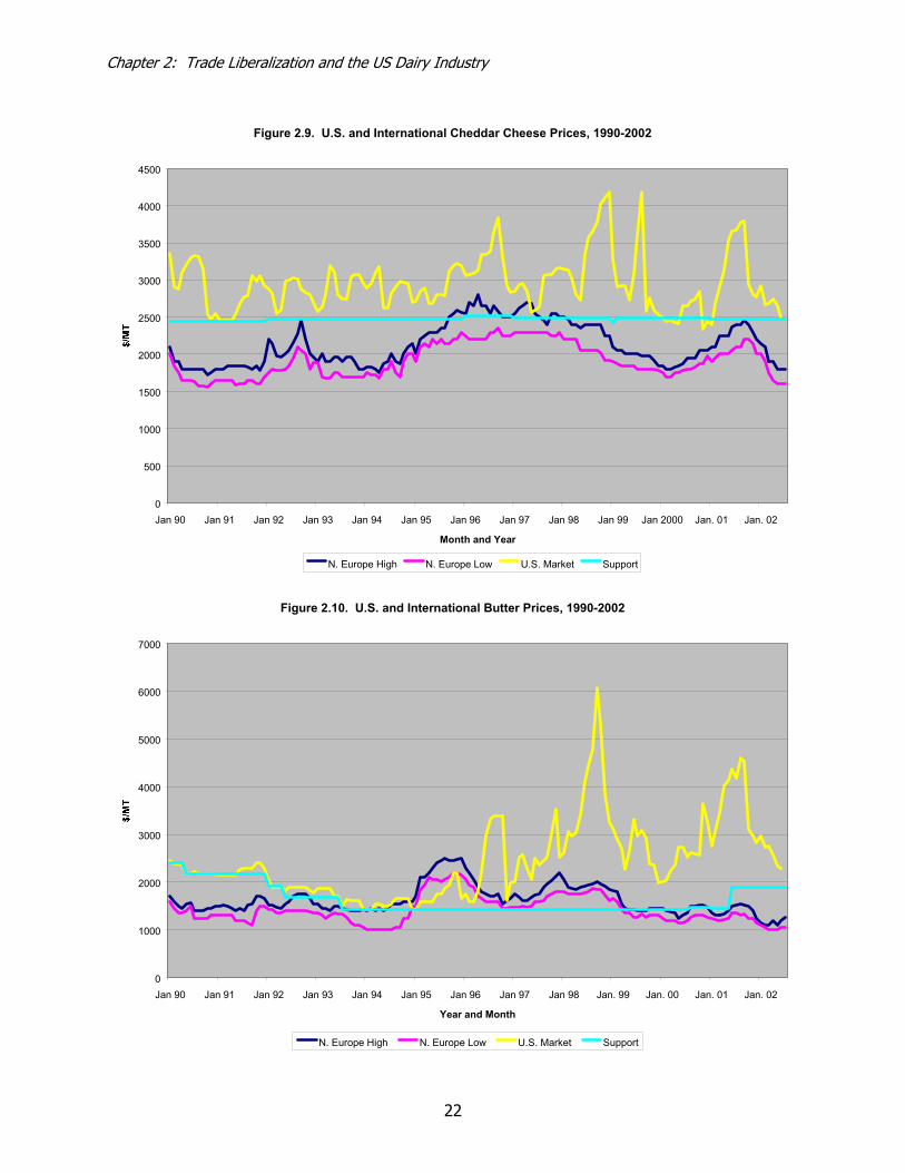
Figure 2.9. US and International Cheddar Cheese Prices, 1990-2002....................... 22
Figure 2.10. US and International Butter Prices, 1990-2002.................................... 22
Figure 2.11. US and International NDM Prices, 1990-2002...................................... 23
Figure 2.12. US and International WMP Prices, 1990-2002 ..................................... 23
Figure 2.13. DEIP Bid Acceptances, 1992-2002 ..................................................... 26
Figure 2.14. Amount of Bonus Payments Under DEIP, 1992-2002 ........................... 34
Figure 3.1. Dantzig’s Transportation Problem ........................................................ 53
Figure 3.2. GAMS Code for Dantzig’s Transportation Problem ................................. 55
Figure 3.3. GAMS Code for a Linear Complementarity Problem ............................... 60
Figure 3.4. GAMS Code for a Nonlinear Complementarity Problem .......................... 64
Figure 3.5. A Simple Tariff Rate Quota.................................................................. 67
Figure 3.6. GAMS Code for an MCP with TRQs....................................................... 69
Figure 4.1. Simplified Conceptual Representation of the World Dairy Trade Model.... 85

vi
List of Tables
Table 2.1. Share of Dairy Exports by Exporting Region and Product, 2000, Quantity Basis ........................................................................... 14
Table 2.2. Value of US Dairy Product Exports, 1990-2002....................................... 15
Table 2.3. Value of US Dairy Product Imports, 1990-2002 ...................................... 16
Table 2.4. Value of US Net Exports of Dairy Products, 1990-2002 ........................... 17
Table 2.5. Main Changes in US Dairy Trade Policy Under the NAFTA and URA.......... 24
Table 2.6. Quantitative Restrictions (TRQs) for US Dairy Product Imports, 2000....... 28
Table 2.7. Summary of Studies on the Impacts of Dairy Trade Liberalization on the US Dairy Industry, 1996-2001................................................... 35
Table 4.1. Model Characteristics Required for Modeling Dairy Trade........................ 76
Table 4.2. Interplant (Intermediate Product) Shipments Allowed in the World Dairy Trade Model........................................................... 86
Table 4.3. Complementary (Equation-Variable) Pairings in the World Dairy Trade Model ............................................................... 87
Table 4.4. Data Requirements for the World Dairy Trade Model.............................. 90
Table 5.1. Dairy Product Designations in the US Dairy Policy Model......................... 96
Table 5.2. Raw Milk Quantity Supplied and Composition, 2001 ............................... 97
Table 5.3. Regional Final Product Demand Estimates, Exports and Imports, 2001 .... 98
Table 5.4. Composition of Intermediate Products from US Plants ............................ 99
Table 5.5. Composition of Selected Imported Products........................................... 99
Table 5.6. Minimum Component Specifications for Final Products.......................... 100
Table 5.7. Component Retention Factors Used to Determine the Yield of Selected Products at US Plants ........................................................................ 101
Table 5.8. Elasticities of Raw Milk Supply, Final Product Demand, US Export Demand and Import Supply ............................................................... 102
Table 5.9. Quota Levels, Ad Valorem Tariffs, Unit Tariffs, Unit Export Subsidy and Export Subsidy Quantity Limitations.................................................... 103
Table 5.10. Processing Costs for Final and Intermediate Products ......................... 104
Table 5.11. Transportation Costs for Raw Milk Assembly and Final Products Distribution.................................................................................... 105
Table 5.12. Transportation Costs for Permitted Intermediate Product Flows........... 106
Table 5.13. Milk Supply, Regional Demand, Import Supply and Export Demand Prices and Data Sources ................................................................. 108

vii
Table 5.14. Summary of Estimated US Dairy Market Impacts of Chapter 4 MPC Imports .................................................................................. 116

Chapter 1: Introduction
1
Chapter 1: Introduction
The US dairy industry accounts for about 12 percent of total farm cash receipts, and is the second largest agricultural sector. After the breakup of the Soviet Union in the early 1990s, the US became the world’s largest producer of cow’s milk. Consumer expenditures on all dairy products exceeded $70 billion during the 1990s, approximately 11 percent of all food expenditures. Furthermore, significant quantities of intermediate dairy products are used as inputs in non–dairy food manufacturing. Clearly, the dairy industry is an important sector of the US economy. Yet, for the past decade, the US share of world dairy exports has averaged much less than 10 percent and exports account for just 2 percent of domestic milk production. Moreover a large percentage of US dairy exports require subsidies to be viable.
Dairy has long been a highly regulated industry in the United States. Since the 1930s, a complex system of federal, state, and local laws and regulations have, to varying degrees, supported prices and regulated how milk and dairy products are sold and distributed. Because domestic prices typically have been set above international price levels, border measures such as quotas and prohibitive tariffs have been necessary to control the flow of imports and protect the integrity of the economic regulations. At the same time, international markets often have been used by the US and other countries to dispose of surplus products—frequently with the assistance of generous export subsidies. This has created the environment in which international dairy prices are volatile and US involvement in world dairy markets has been minimal. The current situation provides a stark contrast to the expressed interest of recent federal administrations and the US Congress for a freer and more open system of international trade.
In recent years, however, the tide has been turning. The dairy industry recently entered a period of domestic and trade policy reform. In particular, three major policy events—the 1994 North American Free Trade Agreement (NAFTA), the 1995 Uruguay Round Agreement (URA),1 and the 1996 Federal Agriculture Improvement and Reform Act (FAIR)2—represent a significant reversal of protectionist policies by opening up
1 The major thrust of the URA was to liberalize international markets. Key provisions for dairy include: (i)
replacement of non-tariff barriers to trade with tariff equivalents and/or Tariff Rate Quotas (TRQs), (ii) reduction of expenditures on export subsidies and the volume of subsidized exports, and (iii) strengthening the minimum access provisions to progressively open protected markets to imports. While the URA permits greater competition from imports, it may also provide significant opportunities for increasing exports of US dairy products and ingredients because of the commitments for trade liberalization made by other countries (particularly the EU) on tariffs, minimum access, and export subsidies.
2 Under the FAIR Act, several policy changes were aimed at reducing government involvement in production and marketing decisions. Key among such provisions are: (i) the phase–out of price supports through government purchases of dairy products by the end of the decade and their replacement with a recourse loan program, (ii) a reduction to 10-14 in the number of marketing orders and reform of the milk pricing system for Grade A milk, and (iii) elimination of marketing assessments (that penalize producers for increasing marketings).

Chapter 1: Introduction
2
markets and limiting government price support. Although the subsequent legislation provided for large direct payments to dairy farmers and the 2002 Farm Bill formalized these over the next few years, the process of trade liberalization is likely to continue and intensify.
In addition, a number of new technologies for separating the components of milk (e.g., fat, protein, lactose) have become commercially viable and other similar technologies will become viable in the near future. This will increase the economic viability of transporting dairy components long distances, and will promote the formulation of new products to better meet the demands of both dairy processing companies and final consumers. Such events will place tremendous pressure on policies aimed at pricing milk and protecting domestic producers. These changes will provide new opportunities for US food companies, both buyers and sellers, to enter international dairy markets and to respond efficiently to world price signals. Much of the analytical research to date fails to account for many of the important facets that determine prices, trade patterns, and competitiveness in the dairy industry today. In general, the existing models are too highly aggregated with respect to regional and product specificity, overly simplistic with respect to policy detail, and naive with respect to the technical relationships and marketing arrangements peculiar to the dairy sector. The overall purpose of this project is to clearly elucidate the issues and areas where analyses are needed, to develop analytical frameworks that allow these important issues to be addressed, and implement an empirical model for the important issue of how imports of product formulations designed to circumvent existing trade barriers can influence outcomes in the US dairy industry.
Recent Trade Policy Changes
The NAFTA and the URA are the two key trade policy reforms for which implementation is essentially complete. US dairy import quotas have increased by roughly 50 percent over 1995 levels by the year 2000 due to the URA. The NAFTA allows Mexico to increase its exports to the US although the volumes involved are relatively small. The market access target set by the URA is 5% of the domestic market although the specific commitments were left to each country’s own discretion and the US, like many other countries, adopted commitments that fall short of the 5% goal. More important is the fact that the strict import quotas of the past have been replaced with tariff rate quotas. Thus, imports are permitted above the quota but at a higher rate of tariff. The URA required that over-quota tariffs be reduced, and these rates are now in the range of 70 to 120 percent for many dairy products. Whether or not imports occur at this rate of tariff depends on the relative difference between internal US prices and world prices. Over-quota dairy imports already occur; high domestic prices have resulted in substantial butter imports during 1997, 1998, and 2001. Also significant is the fact that some products are not subject to quotas or significant tariffs. Imports of these product types (e.g., milk protein concentrates and casein) are increasing, especially for those products that are close substitutes to the more highly protected products. Finally, the

Chapter 1: Introduction
3
URA places limits on certain types of domestic support and the extent to which subsidies may be used to assist exporting activity.
The NAFTA and the URA have fundamentally changed dairy trade policy options for the US As a result, there is a need to better understand the impacts of these agreements before further modifications are made to dairy provisions in the next round of trade negotiations. In particular, one should understand whether current provisions have been beneficial or detrimental, for whom, and by what criteria such determinations are to be made.
Technological Developments in the Dairy and Food Processing Industries
In addition to trade and domestic policy reform, technological developments in the dairy and food processing industries are going to take on a greater importance in the next few years. Current microfiltration technologies permit the fractionation of milk into its basic nutritive components: proteins, fats, lactose and minerals (Rizvi, 1987; Rizvi and Bhasker, 1995). These basic building blocks of milk are already being used to build customized products for industries as diverse as medicine and pharmaceuticals, health foods, and specialized food preparations and ingredients. Component separation and the use of intermediate products3 are ubiquitous in the world dairy industry. Separation allows dairy processing companies to formulate products that can be transported more cheaply, stored for longer periods, and reformulated into a variety of customized food ingredients and value-added products. Already much dairy trade comprises products that can be used by dairy manufacturers in other locations. The implications of future component separation technologies and product formulations for world and US dairy markets has not previously been studied, so the potential impacts currently are unknown.
As new uses are being developed for the components of milk, new dairy products—often intermediate products used to manufacture other dairy or dairy-based products—are being formulated. This creates complications and opportunities in a world where barriers to trade are designed for specific products. A 40-year old example of this in the US dairy sector is casein, a milk protein which can be used as a substitute for dry milk powders in a number of food and non-food products. At the time quotas were established for dairy products, casein was no longer produced in the US nor imported.4 Subsequent to the adoption of section 22 import quotas, food processors discovered that imported casein, for which there was no quota, could be used as a cheaper source
3 ‘Intermediate products’ refer to dairy products used in the manufacture of other dairy products; an
example would be whole milk powder manufactured in New Zealand used for reconstituting fluid milk in Indonesia or Mexico. Manufactured products used in other food industries (such as skim milk powder used in the manufacture of chocolate) can be considered ‘final products’ because their use is ‘outside’ the dairy manufacturing sector.
4 Casein production rapidly declined after the federal Dairy Price Support Program became permanent in 1949 and rendered casein less profitable to make than nonfat dry milk.

Chapter 1: Introduction
4
of milk protein than powders produced in the US The US now imports annually more than $500 million worth of casein and casein derivatives, much of it free of tariffs. As new product types and uses are developed, the ability of product-specific tariffs and quotas to protect domestic producers and processors can be undermined. Due to recent trade agreements, the imposition of new prohibitive tariffs is no longer an option.
Developments in the storage and packaging arena are also contributing to the changing nature of trade patterns. Improved barrier materials and modified atmosphere packaging techniques permit much longer shelf life and therefore the ability to transport perishable products greater distances (Hotchkiss; 1995a, 1995b). Modern warehousing methods and practices along the entire marketing channel are driving changes in dairy product trade, and new technologies allow new marketing practices to be used for dairy products.
In order to analyze these complex and interrelated issues, a suitable modeling framework is required. The next section briefly discusses some of the previously developed models and points out their limitations to address the issues described above.
Review of Analytical Literature
Many interregional models of agriculture and dairy in particular, have been constructed over the past three or four decades (e.g., see Snodgrass and French, 1958; Louwes et al., 1963; McDowell, 1982). Although earlier studies focused on country-level issues, the increased interest in trade over time has seen the development of more international trade applications. Most recently, the Uruguay Round focused attention on agricultural trade and domestic policy reform, and researchers responded with a large number of analyses.
A common aspect of almost all the agricultural trade studies is their derivation from the well-known Samuelson-Takayama-Judge (STJ) modeling framework (Samuelson, 1952; Takayama and Judge, 1964, 1971). Even those models adopting a statistically oriented formulation (as opposed to the linear or quadratic programming approach of STJ) can trace a direct lineage back to the pioneering work of STJ. Given the methodological and algorithmic development spawned by the work of these and other early pioneers, it is quite remarkable that so many contemporary agricultural trade models tend to look just like those of thirty years ago. Many dairy-related analyses employ a standard quadratic programming (QP) model in the quantity domain with linear supply and demand functions, a set of linear conservation-of-flow constraints, and a few fixed per unit transfer costs such as transportation, import tariffs, or subsidies (Lattimore and Weedle, 1981; Baker, 1991; Chavas, Cox, and Jesse, 1993; Cox and Zhu, 1997).
Of the more recent studies undertaken in support of the Uruguay Round, some of most widely referenced include: the Ministerial Trade Mandate (MTM) model by the OECD (1991); the SWOPSIM modeling framework developed at the USDA (see Roningen et al., 1991); the various works of Tyers and Anderson (e.g. 1992); the ongoing efforts of

Chapter 1: Introduction
5
FAPRI (e.g. 1993); and the work by the Food and Agriculture Organization (FAO) of the United Nations with their World Food Model (FAO, 1995). These models all treat dairy as one of many sectors under study; the commodity detail with respect to dairy is therefore negligible. The range of products is aggregated to just fluid milk and manufacturing milk (e.g. OECD/MTM) or, at most, three or four of the major dairy product categories such as fluid milk, cheese, butter, and powder (e.g. SWOPSIM). Although this high degree of product aggregation is required from a practical standpoint in multi-sector, multi-region models, the result is that these models have limited ability to analyze complex interactions among the multitude of products comprising the dairy sector.
Policy instruments in these types of models tend to be very aggregate and non-specific. For instance, the OECD/MTM and SWOPSIM models collapse policy detail to a single measurement of subsidy-equivalents. Although useful, such an approach precludes analyzing the direct impacts of individual policy instruments. These models also tend to ignore bilateral marketing arrangements and agreements. In addition to high degrees of product and geographic aggregation, most previous trade models that include a dairy sector implicitly assume that producers trade directly with consumers. This ignores the crucial role of intermediate dairy products and the processing sector in mediating farm supplies of raw milk and consumer demands for final products.
International trade models generally make the simple assumption that goods moving by ocean freight in international markets will encounter a flat transportation rate per unit of distance. However, this is far from the case. Although there are no publicly available ocean transportation rates for dairy products, we were able to obtain actual ocean freight rates for shipments of dairy products from Oceania ports to global destinations during a recent year. The shipment cost per unit distance for butter and whole milk powder shipped from Oceania to worldwide ports varies substantially. Although the rates per unit distance for butter decline at longer distances, they are also determined by many other important factors. Rates per unit distance are related to the commodity being transferred, wharf charges specific to the origin and destination ports, insurance rates, fuel surcharges and general state of the transportation economy. Also important is whether the shipper participates in a conference scheme5. The rates vary by about 300% from low to high for butter and by about 200% for whole milk powder, even for countries within 500 miles of one another. The variations in the actual rates are large enough to alter the results of any study that makes a naive, flat rate assumption.
Perhaps most important for analyses of product-specific trade policies, most models have not included explicit representation of discriminatory ad valorem tariffs (i.e., tariffs that differ by country of origin). This is a remarkable omission in models designed to explore the impacts of trade liberalization, given the important recent role of tariffication in that process. One reason for the omission is the additional difficulty in formulating and solving models with discriminatory ad valorem tariffs. Takayama and 5 A ‘conference scheme’ is an agreement among shipping companies about rates to be charged.

Chapter 1: Introduction
6
Judge (1971) noted that optimization methods such as QP could not be used to solve models with discriminatory ad valorem tariffs, but demonstrated that complementarity techniques could be employed to solve linear models including them.
Recently constructed models that focus on the global dairy sector are those of Cox and Zhu (1997), Bishop et al. (1993, 1994). The Cox and Zhu model is a conventional QP formulation in the vein of STJ with a quantity domain formulation, linear supply and demand functions, and fixed per-unit transfer costs. The Bishop et al. model adopts a more flexible framework making use of the complementarity approach to equilibrium modeling. Both models use a similar level of disaggregation with respect to regional and product specificity, but Bishop et al. explicitly consider intermediate products. Despite the advances they represent, the regional and product specificity of both these models does not allow analyses of the full range of issues discussed above. Both studies are constrained as to their choice of products by the availability of free or inexpensive public domain data. The only complete and consistently compiled source of global production and trade data is that put together by the FAO. Unfortunately, it is quite highly aggregated and focuses more on quantity than on prices.
Most previous modeling efforts offer few specific and detailed analyses of the impacts of proposed policy options on either the US or the international dairy sectors, although refinements continue on some of these models6. There is a strong need to have useful models ‘on-the-shelf’ and ready to perform timely and relevant analyses. The linkages that the URA has created between trade and domestic support policies imply that increased specificity in empirical models is required to adequately analyze policy options. We believe a useful dairy sector model must at a minimum be able to account for a number of important characteristics of international dairy markets. These are discussed in detail in Chapter 4.
Research Objectives
The overall objective of this project is to develop improved analytical frameworks that can be used to examine the impacts of various trade policy options on the US dairy sector, in light of continuing multilateral trade and domestic policy liberalization. These frameworks should contain a high degree of policy specificity, focuses on intermediate and final product disaggregation, and recognize the complexities of dairy marketing channels. Specific objectives are as follows, and the portions of this report addressing them are indicated in parentheses:
1) Describe the recent history of US dairy imports and exports, i.e., volume, value, level of export subsidies and import protection, by product types. Place the US in a global context with respect to trade and identify the product groups for which trade is contracting, stagnant, and growing. (Chapter 2)
6 For example, the MTM model has evolved to the AGLINK model that includes greater product
disaggregation and policy specificity. Because it does not have partner to partner flows, however, it cannot easily deal with TRQs and targeted export subsidies.
Chapter 1: Introduction
7
2) Describe the current nature of production and trade in the international dairy sector on a disaggregated product basis. Document the current policy regimes and explain the nature of proposed and potential reforms. Explain and quantify the institutional structures which influence trade and production patterns. (Chapter 2)
3) Review the literature pertaining to modeling international dairy trade and other trade literature with an emphasis on how trade liberalization has or will influence the US dairy industry. (Chapters 1 and 2)
4) Formulate mixed complementarity models of the US and world dairy industries. The models describe a farm milk production sector, processing and marketing intermediaries, and final consumption for a wide range of product types and regions. They incorporate all significant policy instruments and contain endogenous prices and quantities. (Chapters 3, 4 and 5)
5) Implement an empirical model of the US dairy industry to estimate the impacts of (new) products formulated to circumvent US trade barriers, using milk protein concentrates (MPC) as an important current example. Estimate the effect of MPC imports on US farm milk production and producer milk prices. (Chapter 5)
Chapter 1 References
Baas, H. J. A., A. J. van Potten, M. R. I. A. Wazir, and A. C. M. Zwanenberg. 1998. The World Dairy Market. Utrecht, Netherlands: Rabobank International.
Baker, A.D. 1991. An Investigation of the Dairy Subsector Impacts of a Free Trade Agreement Between Canada and the United States. Unpublished Ph.D. Dissertation, The Pennsylvania State University, University Park, Pennsylvania.
Bishop, P.M. and A.M. Novakovic. 1994. The Potential Impact of GATT-Induced Policy Reforms on the Dairy Foods Sector of the European Union. Presented at the “Food Policies and the Food Chain: Structures and Inter-Relationships” conference, the 36th Seminar of the European Association of Agricultural Economists, The University of Reading, UK, September 19-21, 1994.
Bishop, P.M., J.E. Pratt, and A.M. Novakovic. 1993. Using a Joint-Input, Multi-Product Formulation to Improve Spatial Price Equilibrium Models. SP 94-06, Department of Agricultural, Resource, and Managerial Economics, Cornell University, 1994. Presented at the “New Dimensions in North American-European Agricultural Trade Relations” conference, Calabria, Italy, June 20-23, 1993.
Bishop, P.M., J.E. Pratt, and A.M. Novakovic. 1993. Analyzing the Impacts of the Proposed North American Free Trade Agreement on European-North American Dairy Trade Using a Joint-Input, Multi-Product Approach. Department of Agricultural, Resource, and Managerial Economics, Cornell University. [Staff Paper No. 93-17]
Burfisher, M. E. and E. A. Jones (eds.) 1998. Regional Trade Agreements and U.S. Agriculture. USDA, Economic Research Service, Market and Trade Economics Division, November. [Agricultural Economic Report No. 771]
Chapter 1: Introduction
8
Chavas, J.P., T.L. Cox, and E. Jesse. 1993. Spatial Hedonic Pricing and Trade. No. 367 Agricultural and Applied Economics Staff Paper Series, University of Wisconsin, Madison, August.
Cox, T.L. and Y. Zhu. 1997. Assessing the Impacts of Liberalization in World Dairy Trade. No. 406 Agricultural and Applied Economics Staff Paper Series, University of Wisconsin, Madison, January.
Dirske, S.P. and M.C. Ferris. 1995. “The PATH Solver: A Non-Monotone Stabilization Scheme for Mixed Complementarity Problems.” Optimization Methods and Software, 5:123-159.
Ferris, M.C. and J.S. Pang. 1995. Engineering and Economic Applications of Complementarity Problems. MP-TR-95-07, Computer Sciences Department, University of Wisconsin, Madison, May.
Ferris, M. C., and T. S. Munson. 1998. “Complementarity Problems in GAMS and the PATH Solver.” Paper Presented at the Computation in Economics, Finance and Engineering: Economic Systems (CEFES) Conference, Cambridge, England, July.
Food and Agricultural Policy Research Institute (FAPRI). 1993. FAPRI 1993 World Agricultural Outlook. Staff Report No. 2-93, Iowa State University, Ames, IA.
Food and Agriculture Organization (FAO) of the United Nations. 1995. Impact of the Uruguay Round on Agriculture: Methodological Approach and Assumptions. ESC/M/95/1, Rome, April.
Griffin, M. 1998. “The Effect of Agricultural Trade Liberalization on Global Dairy Markets.” Paper presented at the 11th Annual Agra Europe European Dairy Conference, London, 25-26 November 1998.
Hashimoto, H. 1984. “A Spatial Nash Equilibrium Model,” in Spatial Price Equilibrium: Advances in Theory, Computation, and Application, P.T. Harker (editor), Springer–Verlag, 1984.
Hotchkiss, J.H. 1995a. Modified Atmosphere Processing of Dairy Products. Paper presented at the annual meeting of the International Association of Milk Regulatory Agencies.
. 1995b. “Overview of Chemical Interactions Between Food and Packaging Materials.” In Foods and Packaging Materials–Chemical Interactions. P. Ackermann, M. Jagerstad, and T. Ohlsson, eds. The Royal Society of Chemistry Special Publication No. 162, Cambridge, p.3-11, 1995b
Kolstad, C.D. and A.E. Burris. 1986. “Imperfectly Competitive Equilibria in International Commodity Markets,” American Journal of Agricultural Economics, 68:27-36.
Lattimore, R.G. and S. Weedle. 1981. The Impact of Multilateral Free Trade in Dairy Products. Working Paper, Agriculture Canada, Ottawa.
Louwes, S.L., J.C.G. Boot, and S. Wage. 1963. “A Quadratic Programming Approach to the Problem of the Optimal Use of Milk in the Netherlands.” Journal of Farm Economics, 45:309–317.
McDowell, F.H. (Jr.). 1982. Domestic Dairy Marketing Policy: An Interregional Trade Approach. Ph.D. Thesis, University of Minnesota, December.

Chapter 1: Introduction
9
Organization for Economic Cooperation and Development (OECD). 1991. Changes in Cereals and Dairy Policies in OECD Countries: A Model-Based Analysis. OECD, Paris, 1991.
Rizvi, S. S. H. 1987. “Supercritical Fluid Extraction of Dairy Foods.” New York Food & Life Science Quarterly, 17(3):23–26.
Rizvi, S. S. H., and A. R. Bhaskar. 1995 “Supercritical Fluid Processing of Milk Fat: Fractionation, Scale-up, and Economics.” Food Technology, 49:90-97,100.
Roningen, V.O., J. Sullivan, and P. Dixit. 1991. Documentation of the Static World Policy Simulation (SWOPSIM) Modeling Framework. Staff Report No. AGES 9151, ERS, U.S. Department of Agriculture, Washington, D.C.
Rutherford, T.F. 1992. Extensions of GAMS for Complementarity Problems Arising in Applied Economic Analysis. First Draft, Department of Economics, University of Colorado–Boulder.
Samuelson, P.A. 1952. “Spatial Price Equilibrium and Linear Programming.” American Economic Review, 42:283–303.
Snodgrass, M. and C. French. 1958. “Linear Programming Approach to the Study of Interregional Competition in Dairying.” S.B. 637, Purdue University Agricultural Experiment Station, West Lafayette, IN, May.
Takayama, T. and G.G. Judge. 1964. “An Interregional Activity Analysis Model of the Agricultural Sector.” Journal of Farm Economics, 46:349–365.
. 1971. Spatial and Temporal Price and Allocation Models. North–Holland Publishing Company, Amsterdam.
Tyers, R. and K. Anderson. 1992. Disarray in World Food Markets: A Quantitative Assessment. Cambridge University Press, 1992.

Chapter 2: Trade Liberalization and the US Dairy Industry
10
Chapter 2: Trade Liberalization and the US Dairy Industry1 Introduction As the world’s largest milk producer2, the US dairy industry has often expressed interest in enlarging export markets for US dairy products. Yet as one of the world’s largest consumers of dairy products, the US is also a lucrative export market for the other major dairy countries. Several domestic and international developments have increased interest among the US dairy industry in world markets during the 1990s. One development was the passage of the NAFTA and Uruguay Round (URA) trade agreements in the mid-decade, and their successors, the current “Doha Round” of international trade negotiations now underway. Another development during the 1990s was additional (positive) experience gained by the US dairy industry in export markets. Much of this experience came about because of increases in world market prices for butter and powder in 1995-96 made US exports more competitive. The Dairy Export Incentive Program (DEIP) is also credited with improving the ability of US exporters to move powders, butter and cheese into international markets. Finally, major US companies such as McDonald’s and Pizza Hut have expanded their activities in foreign markets, and have maintained their supply relationships with US dairy companies. As a result of these developments, there is continued interest in understanding the world market for dairy products, and the potential for growth in US exports. At the same time, there has been an increased level of concern about possible negative impacts of past and potential liberalization of dairy product trade. This chapter reviews recent patterns in world dairy product trade and discusses changes in US dairy trade policy during the 1990s. With that background, current and potential trade policy issues can be better understood. To help provide a perspective on future negotiations about dairy trade policy, the available evidence about how trade (and trade liberalization) affects the US dairy industry also is summarized. World Trade in Dairy Products One of the curiosities of dairy trade patterns in the 1990s is that being a large producer doesn’t mean that a country will be a large exporter, and being a major exporter doesn’t necessarily imply that a country will be a large producer. The US is a good example of a large producer whose role in international dairy markets is smaller than its share of milk production would suggest. New Zealand, which produces about as much milk as Wisconsin, is a major player in world markets for many dairy products. Following the dissolution of the former Soviet Union in 1991, the US became the world’s largest milk producer. India, Russia, Germany, and France round out the top five milk 1 This document draws on Trade Liberalization and the US Dairy Industry available at
www.cpdmp.cornell.edu under “Weblets”. 2 The US is the world’s largest producer of cow’s milk. India is the world’s largest producer if buffalo milk
is included, which may be appropriate given that milk from the two species is mixed in dairy processing in that country.

Chapter 2: Trade Liberalization and the US Dairy Industry
11
producing countries (Figure 2.1). Of these five, Germany and France are members of the European Union, which is a large net exporter of dairy products. Our neighbors, Canada and Mexico are well down on the list. Compared to the grain trade, world trade in dairy products is a rather small share of the total volume of milk production, about 8% in 2000 (Figure 2.2). The largest exporters of dairy products are the European Union3, New Zealand, and Australia (Figure 2.3)4. The EU has been a major player in world dairy markets largely because its domestic dairy policies have resulted in surplus production that cannot be consumed domestically, and it relies heavily on export subsidies to sell dairy products in world markets. In contrast, New Zealand and Australia are major exporters because their populations are small relative to their milk production, they have low-cost milk production systems, and they have undertaken aggressive international marketing efforts (assisted by government organizations). The US’ share in world butter, powder and cheese markets is relatively small (Table 2.1), but US exports still totaled nearly $1 billion in 2001. The world’s largest dairy importers (net of intra-EU trade) in 2000 were the EU, Mexico, China and the US (Figure 2.4). China, Mexico, and Brazil are countries with large populations, relatively low milk production per capita, and moderate levels of per capita income. Algeria, the Philippines, and Indonesia share these characteristics. Russia, a large milk producer, is a major butter importer because of the significant decreases in milk production resulting from its transition to a market-oriented economy. The EU and US are major importers because of their large populations and high incomes, which increase the demand for specialty dairy products from other countries. The US in particular is a major importer of cheese, purchasing primarily specialty cheeses from the EU. US Dairy Product Imports and Exports, 1990-2001 Despite its relatively minor role in most international dairy product markets, the US does export important quantities of dairy products. In 2001, US dairy exports totaled $960 million, an amount nearly three times the value of exports in 1990 (Table 2.2). The major products exported by the US in 2000 include whey and modified whey ($136 million), NDM ($190 million), cheese ($162 million), other products derived from dried milk, buttermilk, or whey ($161 million), and ice cream ($86 million). The value of exports in each of these categories has grown rapidly since 1990, assisted by the DEIP
3 The EU currently consists of 15 countries (Austria, Belgium, Denmark, Finland, France, Germany,
Greece, Ireland, Italy, Luxembourg, Netherlands, Spain, Sweden, Portugal, and the UK), but Poland, the Czech Republic, and Hungary will soon join.
4 Note that use of milk equivalents on a butterfat basis will overstate the importance of exports from countries selling more fat-intensive products (e.g., the EU and New Zealand) and understate the importance of exports from countries selling more solids-not-fat intensive products (e.g., the US).

Chapter 2: Trade Liberalization and the US Dairy Industry
12
Figure 2.1. Major Milk Producing Countries, 2001
0
20
40
60
80
100
120
140
160
180
200
Cow Buffalo
Source: FAO Statistical Databases.
Figure 2.2. Dairy Tade and Cow's Milk Production, 1999 and 2000
0
100
200
300
400
500
600
Production Imports Exports
1999 2000
Trade = ~ 8% of production
Source: FAO Statistical Databases.

Chapter 2: Trade Liberalization and the US Dairy Industry
13
Figure 2.3. Dairy Product Exports by Major Region, 2000
0
2
4
6
8
10
12
14
16
EU New Zealand Australia USA Argentina Poland Finland CzechRepublic
RussianFederation
Ukraine
Milk equivalent (butterfat basis), net of intra-EU trade. Source: FAO Statistical Databases.
Figure 2.4. Dairy Product Imports by Major Region, 2000
0
2
4
6
8
10
12
14
16
EU Mexico China US Philippines Japan Brazil Algeria Malaysia Saudi Arabia
Milk equivalent (butterfat basis), net of intra-EU trade. Source: FAO Statistical Databases.
(Scale matches that in Figure 2.3.)

Chapter 2: Trade Liberalization and the US Dairy Industry
14
Table 2.1. Share of Dairy Exports by Exporting Region and Product, 2000, Quantity Basis
Region Butter Cheese NDM Whole Milk Powder
USA 1.1% 3.9% 7.9% 1.9% European Union 21.3% 33.9% 27.6% 37.8% New Zealand and Australia 57.9% 36.7% 29.8% 41.4% Eastern Europe 3.8% 7.4% 9.9% 1.7% Other 17.0% 22.0% 32.7% 19.1%
Source: FAO Statistical Databases. for NDM and cheese. The importance of the US as an exporter of butter has declined since 1990, reflecting in large measure the decrease in Commodity Credit Corporation (CCC) butter stocks during the decade. A growing proportion of US dairy exports went to Mexico and Canada (Figure 2.5), but a majority of sales were made to countries other than the major dairy traders or our neighbors. As noted earlier, the US is also an important importer of dairy products given its population and high per capita income. The value of dairy product imports in 2001 totaled nearly $1.6 billion (Table 2.3). Over 40% of this was for imports of cheese ($746 million). Casein and caseinates accounted for an additional one-third of the value of imports, and imports of milk protein concentrates (MPC) grew rapidly in the late 1990s to account for about 10% of imports. The vast majority of dairy product imports originated in the EU or New Zealand (Figure 2.6.) The total value of dairy imports grew more slowly than the value of dairy exports during the 1990s, increasing about 90% during the decade. In value terms, the US was a net exporter of NDM, whey products, certain cheeses, ice cream, and certain dried milk products in 2001 (Table 2.4). The US was a net importer in value terms of most cheese, casein products, and butterfat in 2001. The composition of US imports provides a starting point to understand why we still buy foreign dairy products in years when milk production has increased and farm milk prices are low. In general, we import primarily dairy products that aren’t produced in large quantities in the US.

Chapter 2: Trade Liberalization and the US Dairy Industry
15
Table 2.2 Value of US Dairy Product Exports, 1990-2002
Product HTS 1990 1995 2000 2001 YTD 20021
% change, 1990-20012
(Million $) Fluid milk, <1.0% fat 040110 3.9 2.2 1.3 1.0 0.8 -70.3%Fluid Milk, 1-6% fat 040120 11.8 14.8 14.1 12.3 9.1 0.1%Fluid Milk and Cream, >6% fat 040130 1.6 4.1 5.0 8.5 5.1 278.3%Powdered milk, fat <1.5% 040210 11.7 115.2 157.4 189.5 68.3 348.3%Powdered milk, fat >1.5% 040221 3.6 25.3 30.6 38.7 14.7 638.1%Sweetened powdered milk, <1.5% fat 040229 8.2 76.6 7.3 17.3 6.1 105.9%Concentrated milk or cream, not sweetened 040291 1.5 1.1 1.0 3.5 1.5 72.9%Sweetened milk or cream 040299 2.1 20.7 3.2 6.3 5.1 183.4%Yogurt 040310 6.9 6.9 4.1 3.9 2.5 -49.3%Buttermilk and other acidified milks 040390 3.6 7.8 4.1 6.3 7.9 -5.1%Whey and modified whey 040410 35.3 93.7 158.6 135.9 106.9 212.2%Milk protein concentrates 040490 3.9 3.9 12.2 8.3 3.7 69.8%Butter and butterfat 040500 111.2 62.6 7.4 5.3 4.3 -91.9%Fresh cheese 040610 1.2 5.1 11.5 20.4 12.5 1445.3%Grated or powdered Cheese 040620 9.5 26.8 45.9 62.8 55.0 368.8%Processed cheese 040630 5.8 20.4 24.5 27.6 22.5 317.7%Blue-veined cheese 040640 0.1 0.5 0.3 0.4 0.2 669.9%Cheddar, Colby and other cheese 040690 22.2 36.6 56.3 50.8 32.1 186.9%Lactose and lactose syrup 170210 16.8 32.8 56.9 74.0 53.8 234.8%Ice Cream and other edible ice 210500 30.0 87.1 91.3 86.4 64.4 121.3%Other products derived from dried milk, buttermilk, or whey 210610 45.6 71.6 135.2 160.7 112.0 159.7%Casein 350110 2.7 5.1 12.7 7.0 1.5 124.1%Caseinates and other casein derivatives 350190 6.1 13.4 36.0 12.1 6.2 305.7%Milk albumin, concentrates of two or more whey proteins 350220 0.0 0.0 7.6 20.4 19.5 NATotal 345.3 734.3 884.5 959.6 615.7 142.2%1 January through September 2002. 2 Percentage change from average of 1990 and 1991 to average of 2000 and 2001. Source: US International Trade Commission. Data are for domestic exports, which includes exports of products produced entirely in the US and exports of foreign products which have been further manufactured in the US. Note: Product categories are not official designations, rather shortened and aggregated names for diverse product categories.

Chapter 2: Trade Liberalization and the US Dairy Industry
16
Table 2.3. Value of US Dairy Product Imports, 1990-2002
Product HTS 1990 1995 2000 2001 YTD 20021
% change, 1990-20012
(Million $) Fluid milk, <1.0% fat 040110 0.0 0.0 0.2 0.3 0.1 NAFluid Milk, 1-6% fat 040120 3.3 0.1 2.5 2.2 1.7 -20.0%Fluid Milk and Cream, >6% fat 040130 7.4 3.8 6.1 11.3 5.3 63.4%Powdered milk, fat <1.5% 040210 0.5 0.5 5.2 7.0 8.0 645.6%Powdered milk, fat >1.5% 040221 1.0 0.9 7.8 10.0 6.7 924.2%Sweetened powdered milk, <1.5% fat 040229 0.0 0.4 1.8 0.1 0.1 NAConcentrated milk or cream, not sweetened 040291 1.0 1.0 1.5 2.8 1.3 67.9%Sweetened milk or cream 040299 3.0 2.3 9.6 10.1 10.1 400.0%Yogurt 040310 0.3 0.0 2.6 3.9 3.1 2097.9%Buttermilk and other acidified milks 040390 0.1 0.0 0.6 0.7 0.6 914.8%Whey and modified whey 040410 0.6 2.9 13.3 11.9 6.6 3453.3%Milk protein concentrates 040490 3.3 23.5 155.4 104.5 94.6 3273.6%Butter and butterfat 040500 3.8 1.4 30.0 85.1 38.0 2000.5%Fresh cheese 040610 0.4 8.2 3.5 4.8 5.0 897.3%Grated or powdered Cheese 040620 5.2 4.7 8.8 9.1 5.1 67.3%Processed cheese 040630 18.9 20.4 20.9 25.6 21.4 20.3%Blue-veined cheese 040640 13.0 17.9 22.6 23.6 16.2 74.8%Cheddar, Colby and other cheese 040690 401.7 498.0 629.7 682.7 518.1 67.8%Lactose and lactose syrup 170210 0.7 0.8 3.3 4.1 2.6 410.8%Ice Cream and other edible ice 210500 0.1 2.4 17.6 16.8 15.8 11520.6%Other products derived from dried milk, buttermilk, or whey 210610 3.9 11.2 10.2 8.1 6.0 94.7%Casein 350110 305.5 318.6 346.6 328.3 199.6 21.3%Caseinates and other casein derivatives 350190 75.9 117.8 153.8 196.8 126.2 154.2%Milk albumin, concentrates of two or more whey proteins 350220 0.0 0.0 34.0 36.4 32.1 NA
Total 849.5 1036.7 1487.6 1586.2 1123.9 91.5%1 January through September 2002. 2 Percentage change from average of 1990 and 1991 to average of 2000 and 2001. Source: US International Trade Commission. Data are imports for consumption, which includes which have physically cleared US Customs and entered consumption channels immediately, from bonded warehouses, or from Foreign Trade Zones. Note: Product categories are not official designations, rather shortened and aggregated names for diverse product categories.

Chapter 2: Trade Liberalization and the US Dairy Industry
17
Table 2.4. Value of US Net Exports of Dairy Products, 1990-2002
Product HTS 1990 1995 2000 2001 YTD 20021
% change, 1990-20012
(Million $) Fluid milk, <1.0% fat 040110 3.9 2.2 1.1 0.7 0.7 -76.1%Fluid Milk, 1-6% fat 040120 8.5 14.8 11.6 10.1 7.4 5.9%Fluid Milk and Cream, >6% fat 040130 -5.8 0.3 -1.1 -2.8 -0.2 -45.4%Powdered milk, fat <1.5% 040210 11.2 114.7 152.3 182.5 60.3 341.8%Powdered milk, fat >1.5% 040221 2.7 24.4 22.9 28.7 8.0 573.4%Sweetened powdered milk, <1.5% fat 040229 8.2 76.3 5.5 17.3 6.0 90.3%Concentrated milk or cream, not sweetened 040291 0.5 0.1 -0.5 0.7 0.3 341.9%Sweetened milk or cream 040299 -0.9 18.4 -6.4 -3.8 -5.0 1642.6%Yogurt 040310 6.7 6.8 1.4 0.0 -0.5 -90.7%Buttermilk and other acidified milks 040390 3.6 7.8 3.5 5.6 7.3 -16.5%Whey and modified whey 040410 34.7 90.8 145.3 124.0 100.4 187.6%Milk protein concentrates 040490 0.7 -19.6 -143.2 -96.1 -90.9 -5554.4%Butter and butterfat 040500 107.5 61.2 -22.6 -79.8 -33.7 -167.7%Fresh cheese 040610 0.8 -3.0 7.9 15.6 7.5 1817.7%Grated or powdered Cheese 040620 4.3 22.1 37.1 53.7 49.8 627.7%Processed cheese 040630 -13.2 0.0 3.6 2.0 1.1 -121.1%Blue-veined cheese 040640 -13.0 -17.4 -22.3 -23.2 -16.0 72.5%Cheddar, Colby and other cheese 040690 -379.4 -461.4 -573.5 -632.0 -486.0 61.8%Lactose and lactose syrup 170210 16.0 32.0 53.6 69.9 51.2 228.0%Ice Cream and other edible ice 210500 29.9 84.7 73.7 69.6 48.6 79.1%Other products derived from dried milk, buttermilk, or whey 210610 41.7 60.4 124.9 152.6 106.1 165.5%Casein 350110 -302.8 -313.5 -334.0 -321.2 -198.1 19.7%Caseinates and other casein derivatives 350190 -69.9 -104.5 -117.7 -184.7 -119.9 139.9%Milk albumin, concentrates of two or more whey proteins 350220 0.0 0.0 -26.5 -16.0 -12.6 NA
Total -504.3 -302.4 -603.2 -626.6 -508.2 45.8%1 January through September 2002. 2 Percentage change from average of 1990 and 1991 to average of 2000 and 2001.Source: US International Trade Commission. Net Exports equal
domestic exports less imports for consumption. Note: Product categories are not official designations, rather shortened and aggregated names for diverse product categories.

Chapter 2: Trade Liberalization and the US Dairy Industry
18
Figure 2.5. Value of US Dairy Exports by Region, 1990-2002
0
100
200
300
400
500
600
700
800
1990 1995 2000 2001 YTD 2002
Year
EU NZ AUS Canada Mexico E. Europe Other
Figure 2.6. Value of US Dairy Imports by Region, 1990-2002
0
100
200
300
400
500
600
700
800
1990 1995 2000 2001 YTD 2002
EU NZ AUS Canada Mexico E. Europe Other

Chapter 2: Trade Liberalization and the US Dairy Industry
19
Although the dollar value of dairy imports provides relevant information, it is also useful to consider dairy product imports as a percentage of total domestic dairy component use. Butterfat and skim solids equivalents of US dairy imports were roughly constant from 1990 to 1997 (Figure 2.7). Imports accounted for a relatively small share of US commercial disappearance in those years, around 2%. In 1998, imports of both butter fat and skim solids jumped due to high domestic butter prices (and therefore increased butter imports) and increases in MPC imports. Despite this increase, dairy imports accounted for less than 3% of commercial disappearance in 1999, and this amount fell somewhat in 2000. Although the total amount of components imported is small relative to domestic consumption, imports can have important impacts on US milk and dairy product prices. Although the dollar value of dairy imports provides relevant information, it is also useful to consider dairy product imports as a percentage of total domestic dairy component use. Butterfat and skim solids equivalents of US dairy imports were roughly constant from 1990 to 1997 (Figure 2.7). Imports accounted for a relatively small share of US commercial disappearance in those years, around 2%. In 1998, imports of both butter fat and skim solids jumped due to high domestic butter prices (and therefore increased butter imports) and increases in MPC imports. Despite this increase, dairy imports accounted for less than 3% of commercial disappearance in 1999, and this amount fell somewhat in 2000. Although the total amount of components imported is small relative to domestic consumption, imports can have important impacts on US milk and dairy product prices. Given the proximity of Canada and Mexico, it is also of interest to examine patterns of dairy trade with those two countries. The value of US dairy product exports to Canada has nearly tripled since 1990, and has generally grown faster than Canada’s exports to the US (Figure 2.8). Mexico is the US’ most important export market, but sales have been affected by that country’s economic performance over time. Exports to Mexico peaked in 1993, then declined rapidly due to the devaluation of the peso and subsequent economic recession. US exports to Mexico rebounded in 1997, and grew relatively slowly through 2000. In 2001, exports to Mexico surpassed their previous peak in 1993. US imports from Mexico have been a fraction of the value of imports, and have not grown substantially since 1995 (Figure 2.8). Why do we observe the patterns of dairy trade described in the previous sections? Key economic factors influencing the ability of countries to export dairy products include costs of milk production and dairy product processing, strategic market planning and organizations to facilitate a consistent market presence, and the relationship between milk production potential and population. As noted above, though, trade policies adopted by major producing and importing countries have a great deal of influence on existing patterns of trade. It is often said that international dairy markets are “highly distorted”, that is, that outcomes do not really reflect the basic underlying economic factors mentioned above. The relatively small volume of trade in dairy products means

Chapter 2: Trade Liberalization and the US Dairy Industry
20
Figure 2.7. US Dairy Product Imports, Fat and Skim Basis, 1990-2000
0.0
0.5
1.0
1.5
2.0
2.5
3.0
3.5
4.0
4.5
5.0
1990 1991 1992 1993 1994 1995 1996 1997 1998 1999 2000
Year
0.0%
0.5%
1.0%
1.5%
2.0%
2.5%
3.0%
Milkfat m.e. Skim solids m.e. % of Solids, fat % of Solids, skim
Figure 2.8. Value of US Dairy Trade with Canada and Mexico, 1990-2002
0
50
100
150
200
250
300
1990 1991 1992 1993 1994 1995 1996 1997 1998 1999 2000 2001 YTD2002
YearImports Canada Exports Canada Imports Mexico Exports Mexico

Chapter 2: Trade Liberalization and the US Dairy Industry
21
that these policies can have a relatively large impact on world market prices. The US has not been a consistent major player in the “commodity” dairy product markets (butter, NDM, WMP, and cheese) because the Dairy Price Support Program (DPSP) and import restrictions maintain domestic prices higher than world prices (Figures 2.9, 2.10, 2.11, and 2.12). The level of world prices, in turn, is largely a reflection of the policies of key dairy exporters such as the EU (although US policies play a role as well). When world prices approach US prices, interest in exporting grows. When world prices fall, however, interest in exporting these commodities wanes, and as a result US exporters do not acquire as many long-term supply relationships with foreign buyers. The need to maintain a consistent market presence is one of the benefits of the continuation of DEIP. Trade Liberalization and US Dairy Trade Policy, 1990-2001 As early as the mid-1980s, there was a growing recognition of the potential benefits to be gained by liberalization of agricultural trade. Thus, the Uruguay Round of trade negotiations that began in 1986 explicitly included agricultural trade as a main agenda item. The relatively slow progress of these negotiations on agriculture and the successes of the Canada-US Trade Agreement (CUSTA) in the late 1980s encouraged the US, Canada, and Mexico to undertake separate negotiations to liberalize trade, including agricultural products. These negotiations culminated with the North American Free Trade Agreement (NAFTA), which came into force in 1994. The Uruguay Round Agreement (URA) became effective in 1995, and represented a significant step in opening up trade in agricultural products. In addition, the URA created a broader set of trade commitments and the World Trade Organization (WTO) to monitor compliance and arbitrate disputes. To understand the implications of these agreements, it is useful to make a distinction between “trade liberalization” and “free trade”. These two terms sometimes are used as if they meant the same thing, but in practice they often imply very different outcomes. Free trade can be viewed as what results when all barriers to trade (quotas, tariffs, licensing arrangements, administrative requirements, government trading organizations, etc.) are removed, and products can move freely between countries. In contrast, trade liberalization is the process by which some or all of these barriers are reduced but not eliminated. Under trade liberalization, there may be increased opportunities for trade, but substantial barriers to trade may remain. As discussed subsequently, the two trade agreements represent the range of outcomes from essentially free trade in dairy products (with Mexico under NAFTA) to limited increases in opportunities for dairy trade (under the URA). For both agreements, it is important to note that although benefits from liberalizing agricultural trade are likely when producers, processors and consumers are considered together, there is no guarantee that any one of these groups (or producers of a particular commodity like milk) will benefit from the reduction of trade barriers. The main changes under NAFTA and the URA are summarized in Table 2.5.
Chapter 2: Trade Liberalization and the US Dairy Industry
22
Figure 2.9. U.S. and International Cheddar Cheese Prices, 1990-2002
0
500
1000
1500
2000
2500
3000
3500
4000
4500
Jan 90 Jan 91 Jan 92 Jan 93 Jan 94 Jan 95 Jan 96 Jan 97 Jan 98 Jan 99 Jan 2000 Jan. 01 Jan. 02
Month and Year
N. Europe High N. Europe Low U.S. Market Support
Figure 2.10. U.S. and International Butter Prices, 1990-2002
0
1000
2000
3000
4000
5000
6000
7000
Jan 90 Jan 91 Jan 92 Jan 93 Jan 94 Jan 95 Jan 96 Jan 97 Jan 98 Jan. 99 Jan. 00 Jan. 01 Jan. 02
Year and Month
N. Europe High N. Europe Low U.S. Market Support

Chapter 2: Trade Liberalization and the US Dairy Industry
23
Figure 2.11. U.S. and International NDM Prices, 1990-2002
0
500
1000
1500
2000
2500
3000
3500
Jan 90 Jan 91 Jan 92 Jan 93 Jan 94 Jan 95 Jan 96 Jan 97 Jan. 98 Jan. 99 Jan. 00 Jan. 01 Jan. 02
Month and Year
N. Europe High N. Europe Low U.S. Market Support
Figure 2.12. U.S. and International WMP Prices, 1990-2002
0
500
1000
1500
2000
2500
3000
3500
4000
Jan 90 Jan 91 Jan 92 Jan 93 Jan 94 Jan 95 Jan 96 Jan 97 Jan. 98 Jan. 99 Jan. 00 Jan. 01 Jan. 02
Month and Year
N. Europe High N. Europe Low U.S. Market

Chapter 2: Trade Liberalization and the US Dairy Industry
24
Table 2.5. Main Changes in US Dairy Trade Policy Under the NAFTA and URA
Policy NAFTA URA
Market Access Converted Section 22 import quotas for Mexico to TRQs. TRQ amount increase each year, and “over quota” tariff rates decrease until TRQs are phased out in 2003 for most products.
Converted Section 22 import quotas to TRQs. TRQ amounts to increase to 5% of domestic consumption by 2001. “Over quota” tariff rate reductions for all agricultural products must average 36%, with minimum reduction of 15% from 1986-88 base period.
Domestic Support Included language encouraging limits on domestic support, but no binding commitments.
Classified domestic policies on the basis of their impact on trade. For “distorting” policies, required a 20% reduction in the value of support by 2001 compared to the 1986-88 base period. Countries could not introduce new programs with significant trade impacts. Non-distorting support programs not limited.
Export Subsidies Included language affirming that, in principle, the two countries should not use export subsidies to sell in each other’s markets, but no binding commitments.
Must reduce value of export subsidies by 36%, and the volume of subsidized exports by 21% compared to one of two base periods. US can maintain DEIP subject to these limits. Export credit and promotion programs unaffected.
Rules of Origin Included specific rules of origin to limit re-exports of dairy products originating in other countries, unless there was substantial transformation of the product
Less relevant due to broad geographic coverage of the URA.
Sanitary and Phytosanitary
Allowed US to maintain current safety standards, as long as these were “scientifically justifiable.”
Separate agreement dealing with food safety, giving additional importance to international standards under the Codex Alimentarius. US standards can be stricter than international standards only if scientifically justified or based on documented risk assessment.
Technical Barriers to Trade
Allowed the US to maintain its product identity standards.
Separate agreement giving additional importance to international standards under Codex Alimentarius, covering packaging, composition, and labeling.

Chapter 2: Trade Liberalization and the US Dairy Industry
25
Prior to the implementation of NAFTA in 1994, US dairy trade policy consisted of significant quantitative restrictions on many dairy product imports, and subsidized or concessional exports of dairy products, particularly when CCC stocks of powder, butter, and cheese became large. Import restrictions, the Section 22 import quotas, were implemented in the early 1950s when they became necessary to ensure the proper functioning of the Dairy Price Support Program (DPSP)5. These quotas not only limited the total amount of dairy product imports to about 2% of US consumption, but often were both product- and country-specific. That is, even if total imports in a given year were below the overall quota amount, individual countries or regions could only export up to their allotted amount. The quotas were quite effective at limiting imports for major commodities, and allowed the DPSP to maintain US dairy product prices above prices in international markets (and producer milk prices higher than they would be otherwise). However, some products were not included in the quotas and had relatively low tariff rates, notably casein (considered an “industrial product”) and MPC (little imported into the US before 1995). The DEIP was announced by USDA on May 15, 1985 to facilitate exports of surplus dairy products from CCC stocks, and has been a feature of US dairy trade policy since that time. Most subsidized exports have been NDM, but in some years butter and cheese have been an important part of DEIP-supported exports (Figure 2.13). The US also funded programs for food aid shipments of dairy products (mostly NDM) to low-income countries and provided export credit guarantees to facilitate dairy product exports. Under NAFTA, the US agreed to eliminate Section 22 import quotas for Mexico as a part of an agreement that will ultimately result in something close to free trade in dairy products6. To allow each country’s producers and processors time to adjust, the agreement provided for the phasing in of greater access to each other’s markets. Under the agreement, a number of Tariff Rate Quotas (TRQs) were established for both the US and Mexico to provide what is termed “market access” for each country’s dairy products into the other’s market. TRQs are quantities of dairy products that can enter the country without tariffs or with low tariff rates. They are presumed to be preferable to quotas that set an absolute limit on imports, because they allow for “over quota” imports, although at higher tariff rates. Each year, the amount of the TRQ is increased to provide greater market access. Imports in excess of these amounts are still subject to tariffs, but these tariffs are to be phased out by 2003 for most products and 2009 for products like NDM. At that point, the TRQs will be effectively eliminated, and there will be no quantitative import restrictions or tariffs on dairy products traded between the US and Mexico.
5 In the absence of these import restrictions, US purchases of supported products (cheese, butter, and
NDM) would have grown unmanageable and would have been supporting dairy producers in exporting countries.
6 For additional information, see Dairy Markets and Policy Issues and Options Leaflet P-14 entitled “NAFTA and the US Dairy Industry” by Outlaw, Knutson, Nicholson and Novakovic, April 1994, at www.cpdmp.cornell.edu.
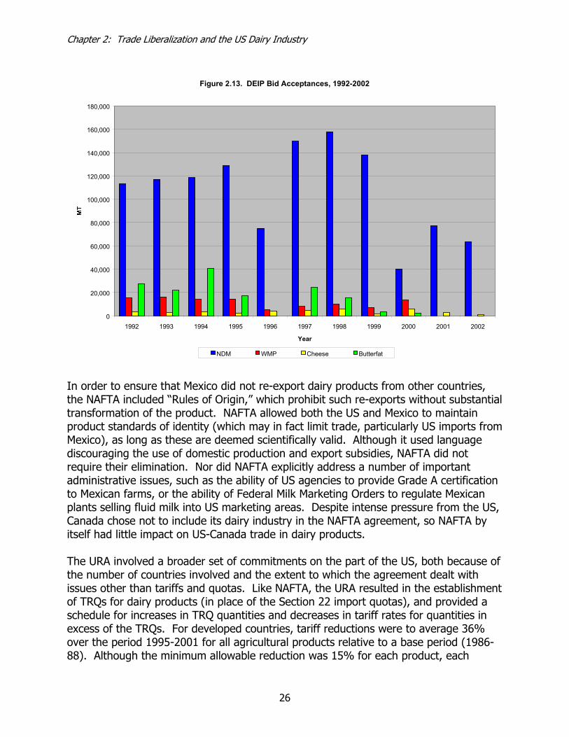
Chapter 2: Trade Liberalization and the US Dairy Industry
26
Figure 2.13. DEIP Bid Acceptances, 1992-2002
0
20,000
40,000
60,000
80,000
100,000
120,000
140,000
160,000
180,000
1992 1993 1994 1995 1996 1997 1998 1999 2000 2001 2002
Year
NDM WMP Cheese Butterfat
In order to ensure that Mexico did not re-export dairy products from other countries, the NAFTA included “Rules of Origin,” which prohibit such re-exports without substantial transformation of the product. NAFTA allowed both the US and Mexico to maintain product standards of identity (which may in fact limit trade, particularly US imports from Mexico), as long as these are deemed scientifically valid. Although it used language discouraging the use of domestic production and export subsidies, NAFTA did not require their elimination. Nor did NAFTA explicitly address a number of important administrative issues, such as the ability of US agencies to provide Grade A certification to Mexican farms, or the ability of Federal Milk Marketing Orders to regulate Mexican plants selling fluid milk into US marketing areas. Despite intense pressure from the US, Canada chose not to include its dairy industry in the NAFTA agreement, so NAFTA by itself had little impact on US-Canada trade in dairy products. The URA involved a broader set of commitments on the part of the US, both because of the number of countries involved and the extent to which the agreement dealt with issues other than tariffs and quotas. Like NAFTA, the URA resulted in the establishment of TRQs for dairy products (in place of the Section 22 import quotas), and provided a schedule for increases in TRQ quantities and decreases in tariff rates for quantities in excess of the TRQs. For developed countries, tariff reductions were to average 36% over the period 1995-2001 for all agricultural products relative to a base period (1986-88). Although the minimum allowable reduction was 15% for each product, each

Chapter 2: Trade Liberalization and the US Dairy Industry
27
country could choose how to reduce tariffs among its agricultural products to achieve the 36% average reduction. The amount of the TRQs were to be set initially at a total of 3% of domestic consumption, to increase to 5% of domestic consumption by 2001. The quantitative restrictions agreed to by the US illustrate the basic approach to tariffication undertaken in implementing its URA commitments (Table 2.6). Fluid milk imports are limited to about 26 million pounds, but face low “in-quota” and “over-quota” tariff rates. Other products, for example fluid milk and cream with a fat content greater than 6% but less than 45%, face tougher import restrictions. Of the TRQ for this and related products, 85% is allocated to one country—New Zealand. Although “in-quota” duties are low, “over-quota” duties are $0.77 per liter, sufficient to be prohibitive under most market conditions. Note that various product categories, sometimes similar and sometimes not, are included in the overall TRQ amount. Also, products containing milk solids—but not typically thought of as “dairy products”—are included in the quantitative restrictions. Thus, there is a TRQ for mixes and doughs for baker’s wares containing more than 25% butterfat by weight. Finally, note that for butter, milk powders, and cheeses, the US still requires import licenses in addition to the other restrictions under the URA. Applicable only to amounts imported under the TRQ, these licenses are typically allocated by country, and their continuation was allowed under the URA despite their potential to limit trade. Note that products not included in the table often face tariffs, but are not subject to quantitative restrictions. The most important of these products are casein and caseinates, milk protein concentrates, and lactose products. Also included in the URA were “special safeguard provisions” that allow the imposition of additional tariffs if the quantity of imports exceeds a trigger level (e.g., greater than 25% of the average of the previous three years), or the c.i.f. price of a product falls below a trigger level (e.g., less than 90% of the average price of the import during 1986-88). For example, if butter from New Zealand were landed in the US at a price of 60 cents/lb, the US could impose an additional tariff of about 17 cents/lb in addition to other tariffs allowed under the TRQ. For volume-based safeguards, the imposition of these tariffs is not automatic, however. The provisions must be approved by the President, and apply only until the end of the calendar year in which they are imposed. In November 2002, USDA announced additional volume-based safeguard tariffs on imports of American cheese, the first such use of safeguards for dairy products. US trade policy for dairy product imports from Mexico follows similar principles, although the product groupings differ, the TRQs will be phased out and no import licenses are required (Table 2.6). Another notable difference under NAFTA at present is that “over-quota” tariff rates differ depending on the value of the product. For lower-value products, a certain dollar amount (a “specific tariff”) is charged, and for higher-value products, a percentage of the value (an “ad valorem tariff”) is assessed. Again, these tariffs will be completely phased out under NAFTA.

Chapter 2: Trade Liberalization and the US Dairy Industry
28
Table 2.6. Quantitative Restrictions (TRQs) for US Dairy Product Imports, 2000
Under Quota Tariff Rates Over-Quota Tariff Rates
Special2
Product TRQ Units Main Country Allocations
General Special1
Import License
Required?
Imports, 2000
Quota Fill Rate
General
(Low Value) (High Value)
TRQs and Tariff Rates Under the URA
Fluid milk, 1-6% fat 11,356,236 Liters None $0.004 Free No 3,547,925 31.2% $0.015 Free --
Fluid milk and cream 6-45% fat, sour cream <45% fat
6,694,840 Liters New Zealand (5,678,117) $0.032 Free No 3,479,823 52.0% $0.772 Free --
Fluid milk and cream, >45% fat; sour cream, >45% fat; butter
6,977,000 Kg None $0.123 Free Yes 6,990,039 100.2% $1.541 to $1.646
-- --
Milk powder, <3.0% fat 5,261,000 Kg None $0.033 Free Yes 3,283,784 62.4% $0.865 -- --
Milk powder, 3-35% fat; Dried sour cream 6-35% fat
3,321,300 Kg None $0.068 Free Yes 1,994,675 60.1% $1.092 --
WMP; dried buttermilk 99,500 Kg None $0.137 Free No 0 0.0% $1.556 -- --
Sweetened or concentrated milk; dry yogurt; modified whey other than WPC; other dairy spreads; other edible fats; chocolate preparations containing butterfat; edible ice; food preparations containing milk solids; milk-based drinks
4,105,000 Kg Australia (1,016,046) Belgium and Denmark (154,221)
3.5 to 20%; $0.029 to
$0.11
Free No 2,176,689 53.0% Varies, but usually
includes both specific and ad valorem
tariff
-- --
Evaporated and condensed milk 6,857,300 Kg Canada (1,028,292); Denmark (610,081); Netherlands (701,707)
$0.022 to $0.039
Free No 5,778,247 84.3% $0.313 to $0.496
-- --
Dried buttermilk and dried whey 296,000 Kg None $0.033 Free Yes 102,983 34.8% $0.876 -- --
AMF and butter substitutes 6,080,500 Kg None $0.154 Free Yes 6,127,634 100.8% $1.996 -- --
Fresh cheeses 48,979,859 Kg EU (25,810,000) ; New Zealand (11,322,000)
10% Free Yes 41,478,029 84.7% $1.509 -- --
Blue-mold cheese (other than Stilton) 2,911,001 Kg EU (2,779,000) 10 to 20% Free Yes 2,822,170 96.9% $2.269 -- --
Cheddar cheese 13,256,306 Kg New Zealand (8,200,000); Australia (2,450,000)
10 to 16% Free Yes 12,716,598 95.9% $1.227 -- --

Chapter 2: Trade Liberalization and the US Dairy Industry
29
Under Quota Tariff Rates Over-Quota Tariff Rates
Special2
Product TRQ Units Main Country Allocations
General Special1
Import License
Required?
Imports, 2000
Quota Fill Rate
General
(Low Value) (High Value)
American-type cheese 3,522,556 Kg New Zealand (2,000,000); Australia (1,000,000)
10 to 20% Free Yes 3,142,708 89.2% $1.055 -- --
Edam or Gouda cheese 6,816,402 Kg EU (6,289,000) 10 to 15% Free Yes 6,719,346 98.6% $1.803 -- --
Italian-type cheeses 13,481,064 Kg Argentina (6,383,000); EU (4,082,000)
7.5 to 25% Free Yes 12,618,655 93.6% $2.146 -- --
Swiss, Emmantaler, or Gruyere cheeses 7,854,833 Kg EU (5,925,000); Switzerland (1,850,000)
6.4 to 10% Free Yes 5,975,078 76.1% $1.386 -- --
Other cheese, including margarine cheese and cheeses containing <0.5% butterfat
1,649,908 Kg New Zealand (1,000,000); EU (425,000)
10% Free Yes 2,640,678 160.1% $1.128 -- --
Chocolate preparations, >5.5% butterfat
26,167,000 Kg Ireland (4,286,491); UK (3,379,297); Australia (2,000,000)
3.5 to 5% Free No 21,483,704 82.1% $.372 to $.582 and
4.3%
-- --
Chocolate preparations, <5.5% butterfat
2,122,834 Kg Ireland (1,700,988); UK (421,845)
3.5 to 10% Free No 0 0.0% $.372 to $.582 and
4.3%
-- --
Mixes and doughs for baker's wares, >25% butterfat
5,398 MT None 10% Free No 4,177 77.4% $0.423 and 8.5%
-- --
Ice cream 5,667,846 Liters Belgium (922,315) and New Zealand (589,312)
10% Free No 1,560,716 27.5% $.502 and 17.0%
-- --
TRQs and Tariff Rates Under NAFTA
Fluid milk and cream, 6-45%, sour cream <45% fat, ice cream
437,000 Liters Mexico (437,000) -- Free No -- $0.094 to $0.123
18.4 to 18.8%
Fluid milk and cream, >45% fat; WMP, sour cream; Butter, AMF, Butter substitutes
51,000 Kg Mexico (51,000) -- Free No -- $0.239 to $0.301
18.8 to 19.1%
Milk powders; dried buttermilk; dried whey
504,000 Kg Mexico (504,000) -- Free No
Not calculated
-- $0.189 to $$0.212
15.6 to 16.8%

Chapter 2: Trade Liberalization and the US Dairy Industry
30
Under Quota Tariff Rates Over-Quota Tariff Rates
Special2
Product TRQ Units Main Country Allocations
General Special1
Import License
Required?
Imports, 2000
Quota Fill Rate
General
(Low Value) (High Value)
Sweetened milk powders; evaporated and condensed milk; dired yogurt; other dried whey products; margarine; chocolate containing butterfat
979,000 Kg Mexico (979,000) -- Free No -- $0.06 to $.223
15.6 to 18.9%
Cheeses 6,626,000 Kg Mexico (6,626,000) -- Free No
Not calculated
-- $0.24 to $0.436
13.9%
1 Within-quota special tariff rates apply primarily to developing countries, and few dairy product imports are received from these countries. 2 Over-quota Special tariff rates for Mexico depend on the value of the product imported, and the designation of low and high value varies for each product
category.

Chapter 2: Trade Liberalization and the US Dairy Industry
31
In addition, the URA called for two other key components: reductions in export subsidies and reductions in domestic support. Because a key cause of international trade in agricultural products is domestic support policies (and often, the product surpluses they create), the URA included language to classify and limit certain types of domestic support. To classify different domestic support policies, the URA employed a system of “boxes” with the names of different colors indicating their relative acceptability under the agreement. In the “blue box” are policies that provide support to agricultural producers by limiting the amount they can produce (e.g., supply controls). This type of support did not have to be reduced, but could not be increased above its 1992 level. “Green box” policies are measures that are deemed to have minimal trade-distorting effects on agricultural production, including government research programs, domestic food aid, direct payments to producers (not tied to level of production) and payments for environmental protection. Green box measures can be used without restriction. Finally, “amber box” measures are those that are deemed to distort market prices, including price supports, direct payments tied to production, and other non-exempt subsidies. The degree of “amber box” intervention is summarized by the “Aggregate Measure of Support” (AMS). Under the URA, the US must reduce its AMS by 20% from the base period (1986-88) by 20017. Countries could maintain their individual support programs subject to the reductions, but they could not implement new support programs that did not exist in the base period. This calls into question whether current policies, such as regional or national dairy compacts would be in compliance with these provisions. The third major component of the URA was reductions in export subsidies. Under the agreement, countries committed themselves to a 36% reduction in the value of export subsidies and a 21% reduction in the volume of subsidized exports by 2001, relative to either a 1986-90 or 1991-92 base period. Countries can maintain their individual export subsidy programs subject to these limits, but may not introduce new export subsidy programs. Export credit guarantees and export promotion programs were exempted from these reductions. In addition to the provisions on market access, domestic support, and export subsidies, the URA brought into existence the WTO as the successor to the General Agreement on Tariffs and Trade (GATT). The WTO differs from GATT in that it is a permanent institutional commitment on the part of signatory countries, deals with services and intellectual property rights as well as goods, and perhaps most importantly, has a more transparent (and presumably binding) dispute settlement mechanism. Two other agreements that are part of the URA are important for dairy trade. The first, dealing with Technical Barriers to Trade (TBT) defines rules to assess the reasonableness of domestic regulatory measures that affect trade. For dairy products, 7 Under what are termed “de minimus” rules, countries are exempted from reductions in product-specific
support that does not exceed 5% of the total value of the product and non-product specific support that does not exceed 5% of the total value of agricultural production.

Chapter 2: Trade Liberalization and the US Dairy Industry
32
this agreement covers packaging, composition and labeling, and processing techniques. The agreement on Sanitary and Phytosanitary (SPS) measures covers health risks (food safety) arising from additives, contaminants, toxins and pathogens in food products. The SPS measures acknowledge the rights of governments to restrict trade in certain products from certain countries in order to protect human, animal, or plant health, but requires that these restrictions be transparent and consistent. Transparency and consistency imply that equal standards are applied to all other countries, and that domestic and foreign products are treated equally. Under the SPS measures, the principle of “equivalence” is given an important role. The equivalence principle states that the US must accept other countries’ SPS measures as “equivalent”, even if they are different than domestic measures, if the foreign SPS measures achieve a level of protection specified as appropriate by the US. Moreover, measures based on international standards are accepted as complying with the SPS agreement. This has given an increasingly important role to the Codex Alimentarius, an international code of standards for human health protection administered by the Food and Agriculture Organization, the World Health Organization, and the Codex Alimentarius Commission. Countries can adopt standards stricter than those accepted by Codex, but these must be scientifically justified or be based on standards deemed appropriate after an appropriately documented risk assessment. Thus, as of 2001, the US dairy trade policy environment had changed dramatically since the early 1990s. The NAFTA had placed the US on the road to something close to free trade in dairy products with Mexico, and the URA had committed the US to reductions in domestic support and export subsidies and increases in market access for dairy products. Moreover, the URA made US product standards and health measures more subject to international scrutiny, and in principle made US trade policy changes subject to dispute settlement rulings by the WTO. Despite (and sometimes because of) these changes, there has been much criticism of trade liberalization, particularly of the perceived imperfections of the URA. One of the main criticisms of the URA has to do with the fact that it does not result in completely free trade. This leads to perceptions that the market access, domestic support and export subsidy provisions have provided greater benefits to countries other than the US. Regarding market access, it is often observed that although TRQs have been established for dairy products, that these quotas may not be filled due to import licenses and other administrative restrictions that prevent quotas from being filled (see Table 2.6 for US TRQ fill rates). In some cases, the tariffs on the TRQ amounts are high enough to discourage imports, and this is often the case for quantities in excess of the TRQ amounts. Reductions in these high “over quota” tariff rates during 1995 to 2001 may not be sufficient to bring about meaningful increases in market access for some countries. Some observers have concluded that the degree of “liberalization” in dairy trade policy actually has been minimal under the URA, but the agreement still serves as an important first step for further reductions in trade barriers.

Chapter 2: Trade Liberalization and the US Dairy Industry
33
Impacts of Trade Liberalization on the US Dairy Industry There are a wide variety of impacts that can be examined related to dairy trade liberalization. Some impacts, such as those on the evolution of domestic farm policy, changes in health risks due to imported dairy products, or the extent to which US dairy product standards have been challenged by international scrutiny, are difficult to quantify. Certainly, the limits imposed by the URA on domestic support policies have influenced the evolution of debates on the 2002 Farm Bill, and limits on export subsidies have played a role in the level of DEIP bonus payments since 1995 (Figure 2.14). Reducing barriers to trade can influence opportunities for growth in milk production and dairy processing, and therefore have potentially important impacts on farm structure, industry concentration, and rural communities. Because the scope for impacts is broad, it is challenging to examine each of them in detail. A starting point for consideration of these broader impacts, however, is an analysis of the basic economic incentives for trade in various types of dairy products, and how these incentives influence milk production, farm milk prices, dairy processing activity, and product prices. This information provides us with greater intuition about the likely longer-term and structural impacts, although detailed studies of these questions would also be beneficial. This section summarizes studies of the economic impacts on the US of liberalization of dairy trade. A variety of studies have been published since the mid-1990s, each with its own objectives and methods (Table 2.7). With one exception, all of the studies listed in the table are ex ante, that is, they attempt to predict future outcomes of ongoing or possible changes in trade policies by the US and(or) other major dairy-producing countries. Most of the studies cited assess the impacts of trade liberalization with a quantitative model that examines outcomes under various trade liberalization scenarios compared to a baseline scenario using the same model. One of the main assumptions about dairy trade liberalization is that it will result in increases in world market prices for dairy, because reductions in domestic support and export subsidies will decrease the amount of subsidized dairy products in international markets. A key question for the US, then, is whether this expected increase in world prices will allow the US to expand its exports, or at least maintain farm milk prices close to current levels. Although many of the studies include a wide variety of variables (milk production, farm prices, product prices, trade patterns), the emphasis here is on changes in farm-level milk prices and dairy farm income given the importance of these two outcomes. One study released in 2001 by the Foreign Agricultural Service of USDA discussed the impacts of the URA on world dairy markets since 1995. Although assessment of the impacts is complicated by developments in foreign markets (such as economic crises in Mexico, Russia, and southeast Asia), FAS concludes that in the absence of the URA’s limitations on export subsidies, more NDM would have been traded on world markets, and NDM prices would have been substantially lower. It attributes the strengthening of

Chapter 2: Trade Liberalization and the US Dairy Industry
34
Figure 2.14. Amount of Bonus Payments Under DEIP, 1992-2002
0
20
40
60
80
100
120
140
160
180
1992 1993 1994 1995 1996 1997 1998 1999 2000 2001 2002
Year
NDM and WMP prices between January 1999 and mid-2001 (Figures 2.11 and 2.12) primarily to the provisions of the URA. Although it does not estimate impacts on US dairy farm income, this report has a generally favorable view of the developments in international dairy markets due to trade liberalization. A number of studies have assessed the impacts of various combinations of past and future trade policy changes related to the URA. These “general dairy trade liberalization studies” were conducted using data from 1992 to 1999. In general, the results of these studies suggest that US dairy producers have little to lose—but importantly, also little to gain—from current or future trade liberalization. A 1996 study (Nicholson) of the impacts of trade liberalization indicated that reductions in tariff rates under NAFTA would provide opportunities for increases in US milk powder exports to Mexico. This study did not examine broader impacts of trade liberalization, and did not fully account for the impacts of peso devaluation on Mexican dairy product imports. A second study (Cox et al.) did examine the impacts of multilateral dairy policy changes under the URA. The results suggested that US farm milk prices would be 0.5% lower in 2000 with the URA than they would have been in its absence. Another study (Larivière and Meilke) predicted that free trade in dairy would have essentially no impact on US milk prices, but that increases in market access to 7% of consumption from the current 5% under URA would result in US milk prices 2% lower than otherwise.
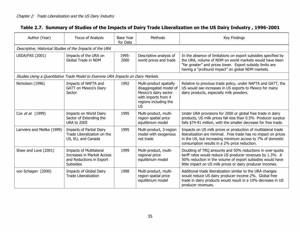
Chapter 2: Trade Liberalization and the US Dairy Industry
35
Table 2.7. Summary of Studies of the Impacts of Dairy Trade Liberalization on the US Dairy Industry , 1996-2001
Author (Year) Focus of Analysis Base Year for Data
Methods Key Findings
Descriptive, Historical Studies of the Impacts of the URA
USDA/FAS (2001) Impacts of the URA on Global Trade in NDM
1995-2000
Descriptive analysis of world prices and trade
In the absence of limitations on export subsidies specified by the URA, volume of NDM on world markets would have been “far greater” and prices lower. Export subsidy limits are having a “profound impact” on global NDM markets.
Studies Using a Quantitative Trade Model to Examine URA Impacts on Dairy Markets
Nicholson (1996) Impacts of NAFTA and GATT on Mexico’s Dairy Sector
1992 Multi-product spatially disaggregated model of Mexico’s dairy sector with imports from 4 regions including the US
Relative to previous trade policy, under NAFTA and GATT, the US would see increases in US exports to Mexico for many dairy products, especially milk powders.
Cox et al. (1999) Impacts on World Dairy Sector of Extending the URA to 2005
1995 Multi-product, multi-region spatial price equilibrium model
Under URA provisions for 2000 or global free trade in dairy products, US milk prices fall less than 0.5% Producer surplus falls $74-91 million, with the smaller decrease for free trade.
Larivière and Meilke (1999) Impacts of Partial Dairy Trade Liberalization on the US, EU, and Canada
1995 Multi-product, 3-region model with exogenous net trade
Impacts on US milk prices or production of multilateral trade liberalization are minimal. Free trade has no impact on prices in the US, but increasing minimum access to 7% of domestic consumption results in a 2% price reduction.
Shaw and Love (2001) Impacts of Multilateral Increases in Market Access and Reductions in Export Subsidies
1999 Multi-product, multi-regional price equilibrium model
Doubling of TRQ amounts and 50% reductions in over-quota tariff rates would reduce US producer revenues by 1.3%. A 50% reduction in the volume of export subsidies would have little impact on US milk prices or dairy producer incomes.
von Schagen (2000) Impacts of Global Dairy Trade Liberalization
1998 Multi-product, multi-region spatial price equilibrium model
Additional trade liberalization similar to the URA changes would reduce US dairy producer income 2%. Global free trade in dairy products would result in a 10% decrease in US producer revenues.
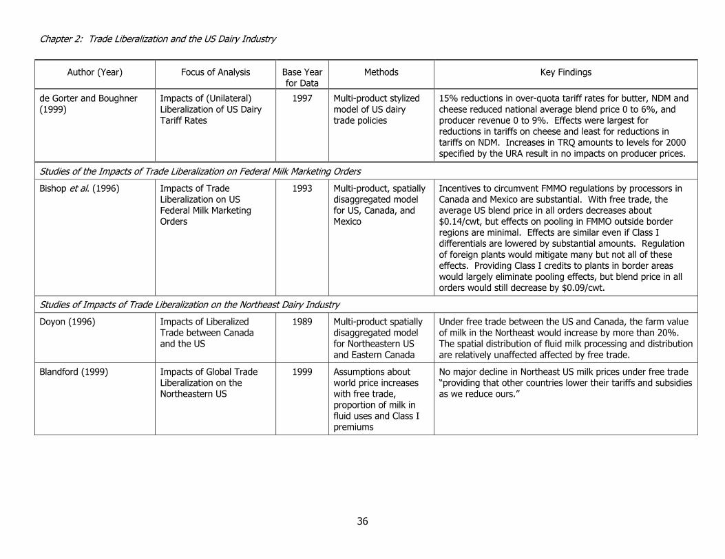
Chapter 2: Trade Liberalization and the US Dairy Industry
36
Author (Year) Focus of Analysis Base Year for Data
Methods Key Findings
de Gorter and Boughner (1999)
Impacts of (Unilateral) Liberalization of US Dairy Tariff Rates
1997 Multi-product stylized model of US dairy trade policies
15% reductions in over-quota tariff rates for butter, NDM and cheese reduced national average blend price 0 to 6%, and producer revenue 0 to 9%. Effects were largest for reductions in tariffs on cheese and least for reductions in tariffs on NDM. Increases in TRQ amounts to levels for 2000 specified by the URA result in no impacts on producer prices.
Studies of the Impacts of Trade Liberalization on Federal Milk Marketing Orders
Bishop et al. (1996) Impacts of Trade Liberalization on US Federal Milk Marketing Orders
1993 Multi-product, spatially disaggregated model for US, Canada, and Mexico
Incentives to circumvent FMMO regulations by processors in Canada and Mexico are substantial. With free trade, the average US blend price in all orders decreases about $0.14/cwt, but effects on pooling in FMMO outside border regions are minimal. Effects are similar even if Class I differentials are lowered by substantial amounts. Regulation of foreign plants would mitigate many but not all of these effects. Providing Class I credits to plants in border areas would largely eliminate pooling effects, but blend price in all orders would still decrease by $0.09/cwt.
Studies of Impacts of Trade Liberalization on the Northeast Dairy Industry
Doyon (1996) Impacts of Liberalized Trade between Canada and the US
1989 Multi-product spatially disaggregated model for Northeastern US and Eastern Canada
Under free trade between the US and Canada, the farm value of milk in the Northeast would increase by more than 20%. The spatial distribution of fluid milk processing and distribution are relatively unaffected affected by free trade.
Blandford (1999) Impacts of Global Trade Liberalization on the Northeastern US
1999 Assumptions about world price increases with free trade, proportion of milk in fluid uses and Class I premiums
No major decline in Northeast US milk prices under free trade “providing that other countries lower their tariffs and subsidies as we reduce ours.”

Chapter 2: Trade Liberalization and the US Dairy Industry
37
The most recent of the studies (Shaw and Love) also suggested that further trade liberalization would have relatively little impact on US farm milk prices. They find that multilateral doubling of TRQ amounts (i.e., to 10% of consumption) and 50% reductions in “over-quota” tariff rates would reduce US dairy farm incomes by about 1%. Perhaps more importantly, their results suggest that further reductions in export subsidies will have little impact on US milk prices or dairy producer incomes. The most pessimistic of the studies—and a bit of an outlier in terms of its overall results—(von Schagen) suggested that further dairy trade liberalization similar to that under the URA would reduce US dairy farm incomes by 2%; free trade is predicted to lower dairy farm revenues by about 10%. A final study (de Gorter and Boughner) indicates the importance of multilateral dairy trade policy changes to the predicted outcomes. Unilateral reductions in “over quota” tariff rates for NDM, butter, and cheese by the US are predicted to reduce dairy producer revenues by as much as 9% depending on which product’s tariff rate is reduced. Although the specific results of these studies do not always agree, their common basic conclusion is that dairy trade liberalization is neither a panacea nor a disaster for US dairy farmers. Other studies have examined specific types of impacts (or impacts on regions within the US). In the mid-1990s, USDA supported a study to examine how trade liberalization would affect the functioning of Federal Milk Marketing Orders (FMMOs). At the time, there was concern that a high degree of trade liberalization, particularly with Mexico, would provide fluid milk processors on both sides of the border with incentives to avoid pooling Class I milk on the orders. A model of Canada, the US, and Mexico with a high degree of spatial and product disaggregation (Bishop et al.) was used to examine whether the size of Class I differentials were high enough to justify the transportation and processing costs necessary to avoid pooling. The study made the important assumption that that sanitary and product identity standards could be met, which means that it provides the highest possible access for fluid milk products, particularly those from Mexico. For its basic scenarios, it assumed that foreign dairy processing plants would not be regulated. The study found that incentives to circumvent FMMO regulations by processors in Canada and Mexico are substantial. Under free trade, nearly 18% less milk would be shipped to fluid plants in the US, and the average blend price across all orders would decrease about $0.14/cwt. Effects were largest for FMMOs bordering Canada and Mexico, and de-pooling outside border regions would be minimal. The study also examined whether reductions in Class I differentials could moderate the effects of trade liberalization, and found outcomes similar to those above even if Class I differentials are lowered by as much as 75%. Using the same model, it was found that Order regulation of foreign plants would mitigate many but not all of these effects. An alternative policy of providing Class I credits (reductions in differentials) to plants in border areas would largely eliminate de-pooling, but the average blend price across orders would still decrease by $0.09/cwt.
Chapter 2: Trade Liberalization and the US Dairy Industry
38
The studies that have been conducted to date suggest that current and future dairy trade liberalization is unlikely to have markedly positive or negative impacts on US dairy farms, at least if the liberalization is undertaken by all the key players in international dairy markets. This may incline some to suggest that further efforts at liberalizing dairy trade are at best not merited, and at worst potentially damaging. However, it is useful to examine the limitations of these analyses before drawing general conclusions about the desirability of dairy trade liberalization. First, most of the models used have relatively short time horizons, that is, they represent better the effects during the first few years after a new policy. This means that they capture less well the potential longer-term adjustments to new trade policies. Thus, they may understate the potential benefits to be gained through trade over the long haul. Second, the number and types of products differs in these models, but in each case product categories are aggregated based on convenience and data availability. This aggregation may mean that the analyses miss growth opportunities for certain products in which the US has a relatively more important share of work markets (e.g., whey products). Third, these models don’t capture the impacts of trade liberalization in other markets (e.g., agriculture more generally, manufacturing, or services). Their analyses are restricted impacts on dairy markets, so they are “partial equilibrium,” not “general equilibrium” models. Thus, they don’t directly explore the broader impacts such as the price of feed grains (which affects milk production costs) and world economic growth (which affects the demand for dairy products). These effects are likely to be important to evaluating the desirability of trade liberalization for the US dairy industry. Fourth, most of the studies focus on the impacts at the farm level, at least for their reported results. Despite the predicted lack of benefits at the farm level, certain groups of US processors and consumers may in fact benefit from dairy trade liberalization. Finally, each of the models explores a limited number of possible policy options. Although in general the ones explored are reasonable, they tend to assume that similar policy changes are required of each trading region. It may be the case the US trade negotiators can achieve concessions for dairy that would be more advantageous than the “one size fits all” types of analyses discussed in the studies8. As a result, these studies provide an important starting point for evaluating dairy trade liberalization, but do not provide definitive answers to the question “Is dairy trade liberalization good for the US dairy industry?” Recent Dairy Trade Issues A number of dairy trade issues have received attention in the US recently, and some of them have implications for the ongoing round of agricultural trade negotiations. Between 1995 and 2000 imports of milk protein concentrates (MPC) grew rapidly. The term MPC is often used, but it is appropriate to distinguish between products produced by ultra-filtration and “dry blends” of powdered milk products made without ultra-filtration. Ultra-filtration is used in processing typical MPC, but there has been a high 8 Of course, it is also possible that the converse occurs.

Chapter 2: Trade Liberalization and the US Dairy Industry
39
degree of concern the use of dry blends to circumvent US tariffs on NDM. In the Harmonized Tariff Schedule (HTS), the key US trade policy document, two types of MPCs are identified. The first includes any complete milk protein that is more than 40% milk protein by weight. The second includes concentrates consisting of greater than 90% casein. The HTS does not distinguish between products made with or without ultra-filtration. The most rapid growth has occurred for MPCs with the lower protein content. One study found that, combined, imports of both types of MPCs equaled about 1.6% of the total protein in US milk production in 2000, or about 1.8% of the casein in US milk production. There were also concerns that they were being illegally used to make “standardized cheeses9,” excessively (but legally) used in cheese starter vats, or at a minimum that they were lowering US prices for NDM and increasing CCC purchases of that product (Harris, 2003). The MPC issue arises because, as noted earlier, MPC are subject to low tariff barriers and no quantitative import restrictions. As a result of the growth in MPC imports, dairy farmer organizations have issued calls for implementation of quantitative and tariff restrictions on MPC, including distinguishing products made with and without ultra-filtration. The General Accounting Office of the US Congress was called in to assess the degree to which MPC might be improperly used in cheesemaking. GAO found relatively little evidence of improper use, noting that MPC have uses in a wide variety of food products. With the change in the butter-powder tilt in 2001 and the general rise in world powder prices over time, incentives for MPC imports have decreased. The volume of MPC imports declined markedly from 2000 to 2001. However, MPC imports remain important because the issue illustrates the dynamic consequences of US commitments to no new trade barriers under the URA. In the past, when new products were developed the US could relatively quickly and easily modify tariff schedules to prevent a surge of imports. This is no longer the case. The impact of MPC imports on US milk prices also has not been fully evaluated to date, and is a focal point for this report (Chapter 5). Another issue that has attracted attention recently is the long-running dispute between the US (joined by New Zealand) and Canada regarding the latter’s dairy export pricing scheme. To comply with its URA obligations, Canada eliminated its previous program of “export levies” (taxes on producers) to pay for subsidized exports of dairy products arising from milk production over the quota amounts specified by its supply management programs. In its place, it implemented a program under which “over production” is paid for and exported at world prices, combined with national pooling of the returns from the domestic and international markets. The US and New Zealand contended this program was an export subsidy that violated Canada’s commitments under the URA. It was important to the US to have a favorable ruling on the case, 9 Use of liquid ultra-filtered milk products within a cheese plant or under special arrangements is
permitted but is under review by FDA. The use of dried ultra-filtered milk products, or fluid ones from other plants is illegal for standardized cheeses such as cheddar and mozzarella. The use of any ultra-filtered products in non-standardized cheese (e.g., pizza cheese) is legal.

Chapter 2: Trade Liberalization and the US Dairy Industry
40
because the EU had begun discussions about implementing a similar program, which would have had more important implications for international dairy markets. In October 1999, a Dispute Settlement Board of the WTO agreed with the US/New Zealand position, and ordered Canada to bring its program into compliance with its obligations. Canada responded by implementing a program similar to the previous one, except that it involved provincial, rather than national, administration and pooling. The US and New Zealand again challenged this program, and in July 2001 another DSB ruled in favor of US/New Zealand, but in late 2001, a WTO appeal board determined that additional information was necessary to reach a decision. This dispute illustrates that despite the lofty goals and apparent transparency of trade liberalization policy under the URA, it often will be necessary for countries to enter into lawsuit-type wrangling over details to obtain an interpretation of what exactly the provisions of the URA imply in particular cases. The Canadian case also reflects issues about the role of what are called State Trading Enterprises (STEs) in international dairy markets. A precise definition of a state trading enterprise is difficult, but includes government or non-government organizations that have been granted exclusive or special rights through which can they influence imports or exports. For dairy products, New Zealand, Canada, and Mexico operated the most important STEs during the 1990s. New Zealand maintained the New Zealand Dairy Board (NZDB), a government-authorized but producer-funded agency that administered all of the country’s dairy product exports. Mexico operated CONASUPO, which controlled and allocated all imports of NDM and WMP. Recent changes have reduced the prominence and potential impacts of these STEs, however. Early in 2001, the NZDB was eliminated in favor of Fonterra. Fonterra is also a producer-owned entity, and will continue to have a large degree of control of dairy exports. However, it does not have the authority to be the sole exporter of dairy products (referred to as the “single desk seller”). Mexico ended the operations of CONASUPO in 1999, and had previously made imported NDM quotas available to a private company. These changes will reduce the impact of STEs on dairy market outcomes, but STEs will still be a likely focal point for the next round of negotiations due to their importance for other commodities, such as wheat. Moreover, there is the issue of whether private organizations with export marketing powers similar to those previously exercised by the government should be considered in the negotiation process. Certainly, the impacts of such private entities may be similar to their government counterparts. A final issue that merits discussion is the role of the application of the SPS agreement to key issues in dairy trade: the use of bST and trade in cheeses made from unpastuerized milk. Despite its approval in the US and some 20 other countries, bST use is not approved in Canada or the EU. As a result, these countries have blocked the approval of maximum residue standards for bST under the Codex Alimentarius, in essence arguing that other factors (such as the health of cows and the potential of increased antibiotic residues in milk) should be considered, not just whether bST residues were present in milk. Approval of a maximum standard for bST would have

Chapter 2: Trade Liberalization and the US Dairy Industry
41
implied that bST was safe, and made countries who refused to import dairy products from countries using it subject to WTO scrutiny. The EU and Canada continue to maintain that the impacts of bST use deserve further study, and a previous ruling on the use of hormones in beef production suggests that some trade barriers may be justified when there is “scientific controversy” about health impacts and “serious” risk analysis has been performed. Although neither the EU nor Canada has banned imports of products from countries using bST, this issue is not yet resolved. France, Italy, and Switzerland produce a variety of cheeses from unpasteurized milk. Each year the EU reports what it considers “unjustified” trade restrictions for these cheeses, including those imposed by the US. Previously, the US had proposed that international standards for cheese under Codex require pasteurization. However, the Codex Committee on Food Hygiene agreed only to mention that pasteurization was one among many methods to ensure the safety of dairy products. Under the “equivalence” principle, countries should be required by WTO to allow imports of unpasteurized cheeses for which risk has been controlled by other means, unless they can provide a scientifically justified risk assessment. If there were a WTO challenge to restrictions on unpasteurized cheese, the outcome is uncertain. Because a number of US states allow the production and sale of unpasteurized cheeses, the US position can be viewed as lacking consistency. On the other hand, the EU would be required to demonstrate that unpasteurized cheeses meet risk standards deemed appropriate by the US. Thus, the interpretation of provisions in the SPS agreement may have important implications for future dairy trade, particularly between the US and the EU. The Future of Dairy Trade Liberalization What are the prospects for further dairy trade liberalization, and what are the negotiating interests of the US? The possibilities for further dairy trade liberalization depend on a variety of factors, including unilateral agricultural policy reform in the EU, the provisions of the 2002 Farm Bill (and any future modifications due to the current budget outlook), world market developments (which influence dairy trade during the negotiating round) and success in negotiating other elements of the agreement. In 1999, EU heads of state reached agreement on reforms to the Common Agricultural Policy (CAP), termed “Agenda 2000”. If the Agenda 2000 policies are implemented as agreed to, intervention (support) prices for dairy products will be reduced by 15% in three equal steps starting in 2005, milk production quotas will be increased by 2.4%, and there will be an increase in direct payments per MT of milk quota. The likely impacts of these policies are to decrease farm milk prices in the EU by about 10%, with similar decreases in dairy product prices, according to a 1999 study. The same study predicted decreases in EU exports of NDM and butter, with increases in EU exports of cheese and WMP. The reforms for dairy are less dramatic than for other agricultural commodities, but their ultimate outcomes will depend on and influence the EU’s position on further dairy trade liberalization.

Chapter 2: Trade Liberalization and the US Dairy Industry
42
The US is keen to achieve further agricultural trade liberalization, not so much because of potential gains to the dairy industry, but because it is a major grain exporter. New Zealand and Australia, for whom dairy products are key agricultural exports, will also be in favor of further reductions in dairy-related trade barriers. In contrast, the EU and Canada will be more lukewarm about trade policy reform for agriculture in general, and perhaps hostile to reforms for dairy specifically, because most studies indicate that reductions in the traditional trade restrictions (tariffs and quotas) would have the largest negative impact on their dairy sectors. In fact, there has been growing interest in “alternative” trade restrictions, including administrative procedures (such as import licensing), and expansion of export credit guarantees. Another potential barrier is modifications of SPS provisions to allow restrictions based on consumer, cultural, and environmental factors, rather than on scientific assessments of risk. Technical barriers to trade (such as requirements on refrigeration, labeling, packaging, and shelf-life) have also been identified by the US International Trade Commission as barriers that prevent US dairy product exports. Finally, the provisions on safeguards (whose use was proposed to address US imports of MPC) may be invoked more in the future as barriers to dairy trade. Various US dairy interests have expressed a strong interest in the reduction or elimination of export subsides, probably because this would force the EU to limit both export subsidies and domestic support, and will be beneficial to US dairy exports. However, each of these “alternative” barriers should be a focus for the current negotiations, in addition to efforts extend the URA provisions with regard to expansion of market access, reduction of domestic support, and decreases in export subsidies. Only one thing is certain: the process of negotiation will be long, and the outcome is uncertain given the both the magnitude of the losses, and highly visible (and sometimes violent) opposition to further trade talks in some countries. Concluding Comments The world’s major economies and trading partners continue to pursue trade liberalization, believing that it will result in greater worldwide economic growth and democratization. The path to greater liberalization of trade contains many obstacles, including those opposed to globalization in general and industry groups that might face losses in sales or income were trade barriers to be reduced in their countries. The prospects for progress on agricultural trade liberalization in the next round are uncertain, despite strong support from the US and others. If trade liberalization does occur, and if it includes dairy trade to a significant degree, the available evidence suggests that the US will not suffer catastrophe, nor will it benefit greatly—at least in the short term. Most studies indicate small decreases in US milk prices under a variety of trade liberalization scenarios (including free trade). This in and of itself may be sufficient to dampen enthusiasm in some segments of the US dairy industry, even as others see themselves as potential winners from greater opportunities for trade. However, it is likely that if there is progress on agricultural trade in general, a future agreement will include dairy. Thus, the US industry should be preparing to provide
Chapter 2: Trade Liberalization and the US Dairy Industry
43
input to US trade negotiators to achieve the best possible terms for the industry, but also prepare themselves to face greater competition from abroad.
Chapter 2 References
Ackerman, K. Z., and P. M. Dixit. 1999. An Introduction to State Trading Enterprises in Agriculture. Market and Trade Economics Division, Economic Research Service, USDA. [Agricultural Economic Report No. 783]
Bailey, K. W. 2001. Imports of Milk Protein Concentrates: Assessing the Consequences. Department of Agricultual Economics and Rural Sociology, The Pennsylvania State University, University Park, PA. [Staff Paper # 343]
Bishop, P. M. and A. M. Novakovic. 1996. The Implications of NAFTA for Milk Marketing Orders. Paper presented at the Tri-National Research Symposium “NAFTA and Agriculture: Is the Experiment Working?” San Antonio, TX, November 1-2, 1996.
Blandford, D. 1999. Globalization and Northeast Agriculture: Implications of the Upcoming Round of World Trade Negotiations. Agricultural and Resource Economics Review, 28(2):128-136.
Cox, T., J. R. Coleman, J.-P. Chavas, and Y. Zhu. 1999. An Economic Analysis of the Effects on the World Dairy Sector of Extending Uruguay Round Agreement to 2005. Canadian Journal of Agricultural Economics, 47:169-183.
de Gorter, H. and D. S. Boughner. 1999. U.S. Dairy Policy and Agreement on Agriculture in the WTO. Canadian Journal of Agricultural Economics, 47:31-42.
Doyon, M. A. 1996. Regional Impact of Dairy Trade Liberalization on the Northeast U. S. and Central Canada Dairy Sectors. M. S. Thesis, Cornell University.
Harris, H. 2003. U.S. Dairy Programs and World Trade Policy Issues, in “Looking Ahead…or Looking Behind?” Proceedings of the 10th Annual Invitational Workshop for Dairy Economists and Policy Analysts. Memphis, TN, April 23-24, 2003. National Institute for Livestock and Dairy Policy.
Larivière, S. and K. Meilke. 1999. An Assessment of Partial Dairy Trade Liberalization on the U. S., EU-15, and Canada. Canadian Journal of Agricultural Economics, 47: 59-73.
Matte, K. L. 1997. Repercussions Down Dairy Lane…The NAFTA/WTO Factor. Journal of Dairy Science, 80:3083-3091.

Chapter 2: Trade Liberalization and the US Dairy Industry
44
Nicholson, C. F. 1996. Economic Liberalization, Free Trade, and Structural Change: A Spatial Economic Analysis of Mexico’s Dairy Sector. Ph.D. Dissertation, Cornell University.
Shaw, I., and G. Love. 2001. Impacts of Liberalizing World Trade in Dairy Products. Australian Bureau of Agricultural and Resource Economics, Canberra, Australia. [ABARE Research Report 01.4]
USDA. Foreign Agricultural Service. 2001. Weekly Market Report: Dairy, Livestock, and Poultry, January 29, 2001. [International Agricultural Trade Report]
US General Accounting Office. 2001. Dairy Products: Imports, Domestic Production, and Regulation of Ultra-filtered Milk. Report to Congressional Requesters, March. [GAO-01-326]
van Schagen, M. 2000. Impacts of Trade Liberalisation on World Dairy Markets. M. S. Thesis, Department of Agricultural Economics and Policy, Wageningen University, The Netherlands.
Chapter 3: Modeling TRQs as a MCP
45
Chapter 3: Modeling Tariff-Rate Quotas as a Mixed Complementarity Problem
Introduction
The use of tariff-rate quotas (TRQs) is widespread, especially in agricultural and other primary sector trade policy settings. Thus, understanding the nuances of TRQs as a trade policy instrument is of critical importance. For example, one question of interest is how further liberalization of trade affect both importing and exporting countries when the volume of that trade is constrained by TRQs. For a net exporting country, analyzing the trade-off between diminished quota rents and increased trade volumes is, potentially, a non-trivial undertaking. What’s more, the problem is made even more difficult because the design and operation of most TRQs is not as straightforward as simple textbook illustrations would imply. Fortunately, many of the extant trade models can be reformulated as mixed complementarity problems (MCPs). They are then capable of being used to analyze even the most complex of TRQ instruments.
It is the purpose of this chapter to demonstrate how complex TRQs can be analyzed within the context of a model formulated as an MCP. This chapter draws upon a number of sources, in particular Ferris and Munson (2000) and Rutherford (1995). Although the primary objective of the paper is to show how TRQs can be analyzed, it also has a secondary objective. That is, to explain some of the jargon associated with optimization models, mathematical programming, and complementarity, and to reveal the role in the economist’s analytical toolbox of models that employ such concepts.
The chapter is organized as follows. We begin with what we call a 10-minute tour through optimization theory. This section culminates with a brief discussion of the Kuhn-Tucker conditions, which enables us to then motivate the complementarity problem. We then change tack and present a series of small models. We start with a simple transportation problem and work up to a spatial price equilibrium model formulated as a mixed complementarity problem, which is coded using the GAMS software. The next section discusses the tariff-rate quota as a policy instrument. We conclude the chapter by bringing it all together, incorporating tariff-rate quotas into a simple 3-region, single commodity trade model. We make extensive use of snippets of GAMS code to demonstrate the models presented in this chapter (Brooke et al., 1998). The models presented herein are well within the dimension limitations of the free version of the GAMS software that can be downloaded from www.gams.com.
The Basics of Optimization
Fundamental to most economic analysis is the notion of optimization; consumers make choices so as to maximize utility, firms seek to maximize profits, nations search for ways to maximize GDP growth, and so on. Moreover, such optimization problems usually have constraints associated with them. For example, consumers maximize utility subject to a budget constraint. In this chapter we focus on models that find optimal solutions to economic problems. The key tools employed to do this fall under the rubric of mathematical programming. To be quite clear at the outset, we are not talking about
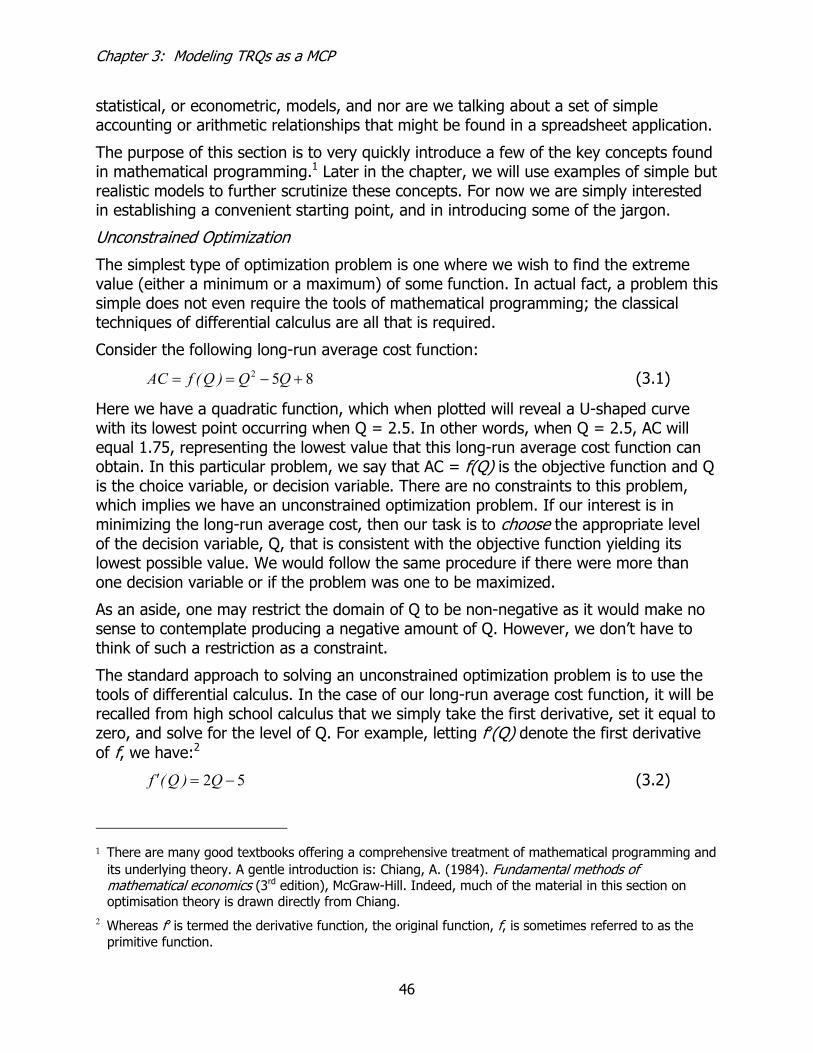
Chapter 3: Modeling TRQs as a MCP
46
statistical, or econometric, models, and nor are we talking about a set of simple accounting or arithmetic relationships that might be found in a spreadsheet application.
The purpose of this section is to very quickly introduce a few of the key concepts found in mathematical programming.1 Later in the chapter, we will use examples of simple but realistic models to further scrutinize these concepts. For now we are simply interested in establishing a convenient starting point, and in introducing some of the jargon.
Unconstrained Optimization
The simplest type of optimization problem is one where we wish to find the extreme value (either a minimum or a maximum) of some function. In actual fact, a problem this simple does not even require the tools of mathematical programming; the classical techniques of differential calculus are all that is required.
Consider the following long-run average cost function:
852 +−== QQ)Q(fAC (3.1)
Here we have a quadratic function, which when plotted will reveal a U-shaped curve with its lowest point occurring when Q = 2.5. In other words, when Q = 2.5, AC will equal 1.75, representing the lowest value that this long-run average cost function can obtain. In this particular problem, we say that AC = f(Q) is the objective function and Q is the choice variable, or decision variable. There are no constraints to this problem, which implies we have an unconstrained optimization problem. If our interest is in minimizing the long-run average cost, then our task is to choose the appropriate level of the decision variable, Q, that is consistent with the objective function yielding its lowest possible value. We would follow the same procedure if there were more than one decision variable or if the problem was one to be maximized.
As an aside, one may restrict the domain of Q to be non-negative as it would make no sense to contemplate producing a negative amount of Q. However, we don’t have to think of such a restriction as a constraint.
The standard approach to solving an unconstrained optimization problem is to use the tools of differential calculus. In the case of our long-run average cost function, it will be recalled from high school calculus that we simply take the first derivative, set it equal to zero, and solve for the level of Q. For example, letting f′(Q) denote the first derivative of f, we have:2
52 −=′ Q)Q(f (3.2)
1 There are many good textbooks offering a comprehensive treatment of mathematical programming and
its underlying theory. A gentle introduction is: Chiang, A. (1984). Fundamental methods of mathematical economics (3rd edition), McGraw-Hill. Indeed, much of the material in this section on optimisation theory is drawn directly from Chiang.
2 Whereas f′ is termed the derivative function, the original function, f, is sometimes referred to as the primitive function.

Chapter 3: Modeling TRQs as a MCP
47
which, when set equal to zero, yields Q = 2.5.
This problem is easy because the function is quadratic, which means that it only has one turning point. A slightly more complicated problem is a cubic function, which has two turning points. For example,
83612 23 −+−== xxx)x(fy (3.3)
Taking the first derivative and setting it equal to zero yields two “roots”, or levels at which f′(x) = 0; namely x = 2 and x = 6. But now we need to determine which of these roots is associated with the maximum point and which is the minimum – we know that a cubic function will have one of each. We do this by taking the second derivatives, i.e. the first derivative of the first derivative. Armed with this information, we can then determine which way the function, f(x), is turning as x approaches 2 and 6. In other words, is the function concave or convex at these points? We will cease this exposition at this point as it can be reviewed in any elementary calculus textbook. Suffice it to say that the theory of unconstrained optimization generalizes to nth-degree polynomial functions.
Before turning to constrained optimization though, it is worth noting a couple of final points. First, one needs to be careful about referring to extreme points as maximum or minimum points of the primitive function. They should more properly be referred to as relative (or local) extrema, as a function may have several extreme points, some of which may be maxima while others are minima. Only one of each can be the global (in contrast to the local) maximum or minimum. And some points at which the first derivative equals zero may fall into a third category, points of inflection.
Second, differential calculus has been used to derive a universal set of necessary and sufficient conditions. These conditions, or rules, can easily be applied to any function to determine the status of all stationary points. That is, all points where the first derivative or the slope of the function is zero. The necessary conditions are based on the first derivatives and are therefore referred to as the first-order conditions. Likewise, the sufficient conditions are based on the second derivatives, and are referred to as second-order conditions.
Optimization With Equality Constraints
It is nearly always the case in economics that some limiting factor(s) impinges upon the choices we are able to make when trying to solve any given optimization problem. An obvious example is when firms set out to maximize profits; they are constrained by the need to employ the available technology. Hence it is necessary to have a technique available for solving constrained optimization problems. The standard method is that of Lagrange multipliers. The essence of the Lagrange multiplier method is to convert the constrained optimization problem into a form where the first-order conditions of the unconstrained problem can still be applied.
By way of example, consider the utility function
121 2xxxU += (3.4)
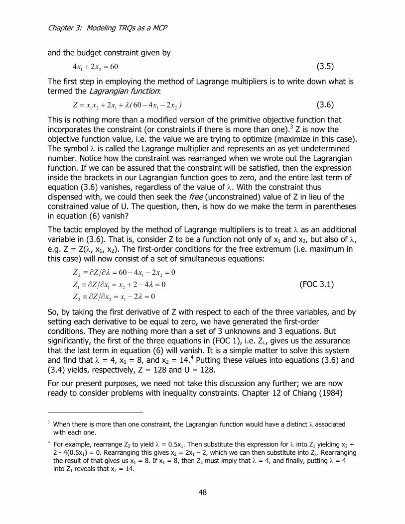
Chapter 3: Modeling TRQs as a MCP
48
and the budget constraint given by
6024 21 =+ xx (3.5)
The first step in employing the method of Lagrange multipliers is to write down what is termed the Lagrangian function:
)xx(xxxZ 21121 24602 −−++= λ (3.6)
This is nothing more than a modified version of the primitive objective function that incorporates the constraint (or constraints if there is more than one).3 Z is now the objective function value, i.e. the value we are trying to optimize (maximize in this case). The symbol λ is called the Lagrange multiplier and represents an as yet undetermined number. Notice how the constraint was rearranged when we wrote out the Lagrangian function. If we can be assured that the constraint will be satisfied, then the expression inside the brackets in our Lagrangian function goes to zero, and the entire last term of equation (3.6) vanishes, regardless of the value of λ. With the constraint thus dispensed with, we could then seek the free (unconstrained) value of Z in lieu of the constrained value of U. The question, then, is how do we make the term in parentheses in equation (6) vanish?
The tactic employed by the method of Lagrange multipliers is to treat λ as an additional variable in (3.6). That is, consider Z to be a function not only of x1 and x2, but also of λ, e.g. Z = Z(λ, x1, x2). The first-order conditions for the free extremum (i.e. maximum in this case) will now consist of a set of simultaneous equations:
02
04202460
122
211
21
=−=∂∂≡=−+=∂∂≡
=−−=∂∂≡
λλ
λλ
xxZZxxZZ
xxZZ (FOC 3.1)
So, by taking the first derivative of Z with respect to each of the three variables, and by setting each derivative to be equal to zero, we have generated the first-order conditions. They are nothing more than a set of 3 unknowns and 3 equations. But significantly, the first of the three equations in (FOC 1), i.e. Zλ, gives us the assurance that the last term in equation (6) will vanish. It is a simple matter to solve this system and find that λ = 4, x1 = 8, and x2 = 14.4 Putting these values into equations (3.6) and (3.4) yields, respectively, Z = 128 and U = 128.
For our present purposes, we need not take this discussion any further; we are now ready to consider problems with inequality constraints. Chapter 12 of Chiang (1984)
3 When there is more than one constraint, the Lagrangian function would have a distinct λ associated
with each one. 4 For example, rearrange Z2 to yield λ = 0.5x1. Then substitute this expression for λ into Z1 yielding x2 +
2 - 4(0.5x1) = 0. Rearranging this gives x2 = 2x1 – 2, which we can then substitute into Zλ. Rearranging the result of that gives us x1 = 8. If x1 = 8, then Z2 must imply that λ = 4, and finally, putting λ = 4 into Z1 reveals that x2 = 14.
Chapter 3: Modeling TRQs as a MCP
49
covers optimization with equality constraints in much greater detail and is worth reviewing. For example, it covers such topics as the interpretation of the Lagrange multiplier, the n-variable and m-constraint case, second-order conditions, and the significance of testing for concavity and convexity.
Optimization with Inequality Constraints
Thus far in our quick tour through optimization theory we have been able to confine ourselves to using the methods of classical optimization, i.e. techniques based on differential calculus. In order to tackle problems with inequality constraints, and for some other reasons that will become obvious shortly, we now need to move into the realm of nonclassical methods. Mathematical programming, which includes (among other topics) linear programming, nonlinear programming, and complementarity methods, is the name given to this collection of nonclassical solution techniques. Clearly the introduction of inequality constraints enables more interesting and realistic problems to be contemplated.
The specific models we get to later in the chapter deal with problems containing inequality constraints. Hence we will not belabor their presentation at this juncture. What we wish to do in this section is introduce the Kuhn-Tucker conditions, and then provide a brief introduction to the mixed complementarity problem.
The types of problems encountered in classical optimization have three key characteristics:
• They contain no explicit restrictions on the sign of the choice variables;
• They contain no inequality constraints; and
• The first-order conditions for a relative or local extremum is simply that the first partial derivatives of the Lagrangian function with respect to all choice variables and the Lagrange multipliers be zero. In other words, we are restricted to situations where there are no boundary or corner solutions. Stated differently, we have only interior solutions.
Mathematical programming methods enable us to find solutions to problems where one or all of these characteristics are not present.
The Kuhn-Tucker Conditions
The single most important result in nonlinear programming is the Kuhn-Tucker conditions (Kuhn and Tucker, 1951). These conditions can be thought of as the nonlinear programming equivalent of the classical first-order conditions. As we shall see, the Kuhn-Tucker method generalises the first-order conditions for an equilibrium to a set of boundary conditions for finding an equilibrium. But unlike those classical conditions, the Kuhn-Tucker conditions cannot be accorded the status of necessary conditions, unless a certain proviso is satisfied.5 However, in specific circumstances, the
5 That proviso is called the constraint qualification. It imposes a certain restriction on the constraint
functions of a nonlinear program so that irregularities on the boundary of the feasible set don’t

Chapter 3: Modeling TRQs as a MCP
50
Kuhn-Tucker conditions turn out to be sufficient conditions, or even necessary and sufficient conditions as well.
At this point we are going to do little more than present the derivation of the Kuhn-Tucker conditions. Their relevance will become clearer later in the chapter. Our primary reason for presenting them at all is because they provide a bridge from the theory of constrained optimization to the mixed complementarity problem.
Consider the following generic optimization problem, which incorporates two constraint functions and explicit nonnegativity conditions:
( )( )( )
0
321
23212
13211
321
≥≤
≤
=
x,x,xrx,x,xgrx,x,xgsubject to
x,x,xfMaximise π
(NLP 3.1)
We can imagine that f and g1, say, are nonlinear functions. Hence we call this problem (NLP 3.1) for NonLinear Program. As before, we can write the Lagrangian function for this problem:
( ) ( )( ) ( )( )3212
22
3211
11
321 x,x,xgrx,x,xgrx,x,xfZ −+−+= λλ (3.7)
The resulting Kuhn-Tucker conditions can be stated compactly as follows (or more accurately, one version of the Kuhn-Tucker conditions, expressed in terms of the Lagrangian function Z, can be stated this way):
2 1,i 0 and 0 0
3 2, 1,j 0 and 0 0
=∀=∂∂
≥≥∂∂
=∀=∂∂
≥≤∂∂
iii
i
jjj
j
Z,,ZxZx,x,
xZ
λλλ
λ
(KT 3.1)
What do these six expressions comprising the Kuhn-Tucker conditions tell us?
First of all, two of the six expressions are nothing more than a restatement of parts of the original problem, i.e. xj ≥ 0 simply restates the nonnegativity conditions for the three primal variables. Similarly, ∂Z/∂λi ≥ 0 reiterates the constraints, i.e. one such condition for each of the two constraints. But notice that associated with each variable type, i.e. the choice variables (xj) and the Lagrange multipliers (λi), there is a corresponding marginal condition that must be satisfied by the optimal solution.6
invalidate the Kuhn-Tucker conditions, should the optimal solution occur at that boundary. While the constraint qualification is important to the theory of nonlinear programming, and to the Kuhn-Tucker sufficiency theorem, we are not going to discuss it in this paper. A nonlinear programming text should be consulted for further information.
6 In case it is not yet apparent, it is worth noting at this point that the first-order conditions, of both constrained and unconstrained optimisation problems, describe a set of equations that must hold true at the equilibrium or optimal solution. They are sometimes thus referred to as the first-order

Chapter 3: Modeling TRQs as a MCP
51
Finally, there is what is known as the complementary slackness conditions, i.e. the last two expressions on each line of (KT 3.1), which simply state that the product of two terms must equate to zero. In other words, each variable is characterised by complementary slackness in relation to a particular partial derivative of the Lagrangian function Z. And what does this mean? It means that for each xj, we must find in the optimal solution that either:
• The marginal condition holds with a strict equality (as in the classical context); or
• The choice variable in question must take on a zero value; or
• Both of the above.
Analogously, for each λi, we must find in the optimal solution that either the associated marginal condition holds as an equality – meaning that the ith constraint is satisfied exactly – or the Lagrange multiplier vanishes, i.e. becomes zero, or both.
It is by exploiting the complementary slackness conditions that it becomes possible to find corner or boundary solutions. Of significance in the case of models that explicitly incorporate tariff-rate quotas, it is the property that enables endogenous regime switching to occur. In fact, short of exploiting complementary slackness, there exists no other way to explicitly model such behavior.7 We will return to this point later.
Before we turn to the mixed complementarity problem, we would point out that the Kuhn-Tucker conditions give rise to a natural economic interpretation. The Lagrange multipliers can be regarded as shadow prices. Thus, the Kuhn-Tucker conditions tell us that, in an optimal solution, when a constraint holds with a strict inequality, then by complementary slackness, the associated shadow price must be zero. Similarly, if an activity level (e.g. a primal variable) is strictly greater than zero, then the associated marginal condition must hold with a strict equality. We will return to this in some detail shortly.
The Mixed Complementarity Problem (MCP)
Now that we have understood the Kuhn-Tucker conditions, we are ready to examine complementarity. A nonlinear complementarity problem consists of a system of simultaneous (linear or nonlinear) equations that are written as inequalities and are linked to bounded variables in a manner that encapsulates complementary slackness relationships. In a mixed complementarity problem (MCP), the equations may be a mixture of inequalities and strict equalities. For more rigorous details and a mathematical definition, see Rutherford (1995).
equilibrium conditions. So, we have two ways to describe the problem; the underlying optimisation problem, and a set of conditions that characterise (i.e. must hold true) a solution to the underlying optimisation problem.
7 There are, of course, techniques for approximating regime switching that don’t require complementarity.

Chapter 3: Modeling TRQs as a MCP
52
It is possible to rewrite (KT 3.1) in accordance with this definition, and thereby transform (NLP 3.1) into an equivalent MCP. However, the generic nature of the problem specified in NLP 3.1 means that the expression for the equivalent MCP may well be confusing for the novice. To avoid this possibility, we would prefer to derive an MCP using a specific example, and shall do so shortly.
Before leaving this section, however, we would make a few general comments relating to MCPs. The underlying theory of complementarity, and the closely related variational inequality was developed in the 1960s, e.g. see Cottle et al., 1992; Lemke and Howson, 1964; Hartman and Stampacchia, 1966. For a thorough review, see Harker and Pang (1990). It was not until much later that commercially available algorithms capable of solving large scale complementarity problems became available, e.g. see Rutherford (1993) and Dirkse and Ferris (1993). The solver we use is called PATH (Dirkse and Ferris, 1993), which is seamlessly linked with the GAMS modeling software (Brooke et al., 1998).
As noted earlier, the equilibrium conditions that characterize an underlying optimization problem are an alternative way of expressing that problem. But there are some problems that can be formulated as an MCP for which there is no equivalent underlying optimization problem. Such problems arise frequently in economics. Hence, the MCP offers the modeller greater choice and flexibility than traditional NLP formulations. A pertinent case in point is the explicit treatment of tariff-rate quotas, which requires a modeling framework able to handle regime switching. For a description of the conditions that give rise to the lack of equivalence between NLPs and complementarity problems, and for some common examples, see Nicholson et al. (1994) and Nagurney et al. (1996a). For a similar discussion in the context of general equilibrium modeling, see Lofgren and Robinson (1999).
Multi-Region Models8
Having reviewed, albeit very briefly, the theory underlying optimization, we now turn to some specific examples. Our purpose here is twofold:
• To practically demonstrate what we’ve been talking about in the previous section; and
• To develop a realistic but simple model that incorporates tariff-rate quotas.
Whether a problem is formulated as a traditional NLP (of which linear problems are just a special case) or as an MCP, it is necessary to be able to then find a solution to the problem. Only in the most trivial of cases will the method of substitution and elimination, which we used earlier, be helpful. The most popular means of specifying and then solving the types of problems we are concerned with here is the GAMS modeling software. GAMS, which stands for General Algebraic Modeling System, 8 We focus on multi-region models in this paper. It should be understood, however, that the same
concepts apply to products (or sectors or markets) and time. In other words, the practical analyzis of space, form, and time amounts to much the same thing.
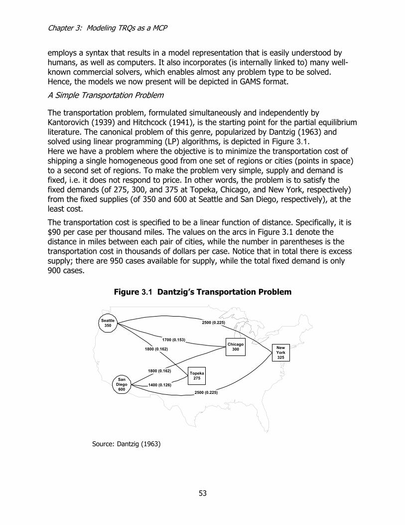
Chapter 3: Modeling TRQs as a MCP
53
employs a syntax that results in a model representation that is easily understood by humans, as well as computers. It also incorporates (is internally linked to) many well-known commercial solvers, which enables almost any problem type to be solved. Hence, the models we now present will be depicted in GAMS format.
A Simple Transportation Problem
The transportation problem, formulated simultaneously and independently by Kantorovich (1939) and Hitchcock (1941), is the starting point for the partial equilibrium literature. The canonical problem of this genre, popularized by Dantzig (1963) and solved using linear programming (LP) algorithms, is depicted in Figure 3.1. Here we have a problem where the objective is to minimize the transportation cost of shipping a single homogeneous good from one set of regions or cities (points in space) to a second set of regions. To make the problem very simple, supply and demand is fixed, i.e. it does not respond to price. In other words, the problem is to satisfy the fixed demands (of 275, 300, and 375 at Topeka, Chicago, and New York, respectively) from the fixed supplies (of 350 and 600 at Seattle and San Diego, respectively), at the least cost.
The transportation cost is specified to be a linear function of distance. Specifically, it is $90 per case per thousand miles. The values on the arcs in Figure 3.1 denote the distance in miles between each pair of cities, while the number in parentheses is the transportation cost in thousands of dollars per case. Notice that in total there is excess supply; there are 950 cases available for supply, while the total fixed demand is only 900 cases.
Figure 3.1 Dantzig’s Transportation Problem
Seattle350
SanDiego
600
2500 (0.225)
1700 (0.153)
1800 (0.162)
1400 (0.126)
1800 (0.162)
2500 (0.225)
Topeka275
NewYork325
Chicago300
Source: Dantzig (1963)

Chapter 3: Modeling TRQs as a MCP
54
In keeping with the style of the previous section, we can state this problem algebraically as follows:
0
≥
∀≥
∀≤
∑
∑
∑∑
ij
ijij
jiij
i jijij
x
jdx
isxsubject to
xcMinimise
(LP 3.1)
Alternatively, we can write the model using GAMS (see Figure 3.2). Except for the line numbers, which have been added for expositional convenience, the code in Figure 3.2 is literally a GAMS program. Not only does it include the algebraic description of the model, lines 36 through 40, it also contains the data used to parameterise the model. Specifically, lines 1-3 specify the sets, or indices, on which the problem’s parameters, variables, and equations are defined, i.e. set i denotes the supply points (Seattle and San Diego), while set j denotes the three demand points. Lines 5 through 13 declare the two parameters, si and dj, and also assigns values to these parameters. It ought to be apparent that si denotes the supply quantities of 350 and 600 available at Seattle and San Diego, respectively. Likewise dj denotes the demand quantities. Lines 15-18 produce a table of distances that is subsequently used in line 23 to calculate the shipping cost associated with each of the six arcs or routes. Lines 25-29 declare the variables. Note that z is just the objective function value. Also note the command in line 29; it is the GAMS-equivalent of specifying the non-negativity condition on the variable xij.
Lines 31 through 34 declare the equations contained in the model, while lines 36-40 specify the algebra of each equation. In GAMS, =e= means strictly equal to, =l= means less than or equal to, and =g= means greater than or equal to (the ≤, =, and ≥ signs are reserved for use in assignment statements). The command in line 42 simply says take all of the equations that have been specified and use them to create a model called transport. Line 44 tells GAMS to solve the model called transport using the LP solver. In other words, the user is telling GAMS that this model is an LP problem.
To recap, what we have specified here is a linear programming problem. An LP is a special case of the NLP class of problems where both the objective function and all of the constraints are linear. Incidentally, if the objective function was quadratic and the constraints were linear, then we would have a problem known as a quadratic programming (QP) problem. LP and QP problems are significant from an algorithmic point of view because specialized solvers are able to solve these problems much more quickly than general NLP solvers can. An NLP may have an objective function that contains nonlinearities of a higher order than quadratic. It may also have linear or nonlinear constraints, or a mixture of both.

Chapter 3: Modeling TRQs as a MCP
55
Figure 3.2 GAMS Code for Dantzig’s Transportation Problem
1 Sets2 i canning plants / seattle, san-diego /3 j markets / new-york, chicago, topeka /;45 Parameters6 s(i) capacity of plant i in cases7 /seattle 3508 san-diego 600 /910 d(j) demand at market j in cases11 /new-york 32512 chicago 30013 topeka 275 /;1415 Table dist(i,j) distance in thousands of miles16 new-york chicago topeka17 seattle 2.5 1.7 1.818 san-diego 2.5 1.8 1.4 ;1920 Scalar f freight in dollars per case per thousand miles /90/;2122 Parameter c(i,j) transport cost in thousands of dollars per case;23 c(i,j) = f * dist(i,j)/1000;2425 Variables26 x(i,j) shipment quantities in cases27 z total transportation costs in thousands of dollars ;2829 Positive Variable x;3031 Equations32 cost define objective function33 supply(i) observe supply limit at plant i34 demand(j) satisfy demand at market j ;3536 cost.. z =e= sum((i,j), c(i,j)*x(i,j));3738 supply(i).. sum(j, x(i,j)) =l= s(i);3940 demand(j).. sum(i, x(i,j)) =g= d(j);4142 Model transport /all/;4344 Solve transport using lp minimizing z;
Source: GAMS model library (trnsport.gms), www.gams.com.
Finally, for the sake of completeness, we should point out that a pure transportation problem such as (LP 3.1) need not be formulated as an LP problem in order to find a solution; there is another whole class of problems called network problems, for which very fast solution algorithms have been designed.
A solution to this problem will generate the quantities shipped (defined by city of origin and destination). The objective, as already noted, is to minimize the total transportation cost. The only constraints to this simple problem are that shipments must be non-negative (they may be zero along a particular route); the supply cities cannot ship more than they have available to ship; and the total quantity of shipments into a demand city

Chapter 3: Modeling TRQs as a MCP
56
must be at least as great as the fixed amount demanded at that city. Given that each case of the good shipped incurs a positive cost, we would expect that this last constraint will be satisfied with a strict equality, i.e. the quantity shipped into a city will exactly equal the quantity demanded at that city.
The solution is as follows:
• Ship 300 cases from Seattle to Chicago;
• Ship 325 cases from San Diego to New York; and
• Ship 275 cases from San Diego to Topeka.
The total transportation cost, z, will be $153,675. This represents an optimal solution, which means that given the fixed supplies, it is not possible to satisfy the fixed demands at a lower total cost. Note that the excess supply of 50 cases remains at Seattle. This problem actually has more than one optimal solution. The per unit shipping cost is identical along both the Seattle-New York and the San Diego-New York routes. Hence, an equally optimal solution would have been the same as above except Seattle could have shipped 50 cases to New York while San Diego could have shipped 275 cases to New York, instead of 325. In this alternative optimal solution, the total transportation cost would still be $153,675 but the excess 50 cases would be located at San Diego.
Finally, formulating and solving this problem as an LP yields two other pieces of valuable information; the shadow price associated with each of the constraints and the marginal cost associated with each variable. While the solution technique enables this information to be generated, it is important to understand that these values, i.e. the shadow prices and the marginal costs, are not explicit variables in the problem being solved.
The shadow prices associated with the two supply constraints are zero. This should not be a surprise as there is excess supply in this problem. The shadow prices represent the value of relaxing the constraint. In other words, how much would the objective function value, z, change if we had one more case at either Seattle or San Diego? The answer is zero because demands are fixed and another case available for supply therefore has no value – anywhere. Recall that the shadow prices are akin to the Lagrange multipliers.
The shadow prices associated with the three demand constraints are 0.225, 0.153, and 0.126 at New York, Chicago, and Topeka, respectively. What does this mean? Consider the New York demand constraint. If New York required 326 cases, i.e. one more than is currently specified, then the objective function value would increase by 0.225 (or, equivalently, the total transportation cost would go up by $225). This, it can be seen, is nothing more than the cost of getting another case from Seattle, the point at which there exists excess supply.
The marginal costs associated with the six variables are zero, except for along the Seattle-Topeka arc where it is 0.036, and along the San Diego-Chicago arc where the

Chapter 3: Modeling TRQs as a MCP
57
marginal cost is 0.009.9 What does this mean? It means that it is optimal to send nothing from Seattle to Topeka and from San Diego to Chicago. But if you insisted on sending just one case along these arcs, it would add $36 and $9, respectively, to the optimal (minimum) total transportation cost.
The Transportation Problem as a Linear Complementarity Problem (LCP)10
There is no compelling reason why the transportation problem shown above should be formulated and solved as a complementarity problem. Nevertheless, we will do it so as to explicitly relate the complementarity problem back to a simple LP. We will then move on to a model that includes price responsive supply and demand functions.
Consider the simple transportation problem as specified in (LP 3.1). As we’ve just seen, this problem can be solved as a linear program. But let’s go back to the theory we discussed earlier. The derivation of the optimality conditions for this problem begins by associating with each constraint a multiplier, alternatively termed a shadow price or dual variable. These multipliers represent the marginal price on changes to the corresponding constraint. Instead of the λs we used earlier, let’s label the prices on the supply constraint ps and those on the demand constraint pd.
Intuitively, for each supply node i we have:
∑≥≤j
ijisi xsp and 0 (3.8)
In other words, supply prices cannot be negative and the quantity available for supply at a particular location must be greater than or equal to the sum of all shipments out of that location.
Consider what happens when si > Σjxij, i.e. supply is strictly greater than the sum of the shipments. In a competitive setting, no rational person would be willing to pay for more supply at location i; it is already oversupplied. Therefore ps at that location would be zero. Alternatively, when si = Σjxij, that is the market clears, one might be willing to pay for some additional supply of the good. Therefore ps ≥ 0. We can write these two conditions succinctly as:
ixspj
ijisi ∀≥⊥≤ ∑ 0 (3.9)
where the “⊥” symbol is understood to mean that at least one of the adjacent inequalities must be satisfied as a strict equality, i.e. either ps = 0 or si = Σjxij. This is nothing more than a formal statement of the complementary slackness result that we saw earlier when presenting the Kuhn-Tucker conditions.
9 Not counting the objective function variable, z, whose marginal cost is zero, there are six variables in
this model, i.e. i = 2 times j = 3 equals 6, and x is defined on i and j. 10 This section draws heavily on Ferris and Munson, 2000.

Chapter 3: Modeling TRQs as a MCP
58
We can go through a similar logic with respect to the demand markets and derive the complementarity relationship:
jdxp ji
ijdj ∀≥⊥≤ ∑ 0 (3.10)
In other words, if shipments into a demand location were to exceed the quantity demanded, then we’d expect the demand price to be driven down to zero.
Also, from basic intuition, we know that the supply price at i plus the transportation cost cij from i to j must exceed the market price at j:
djij
si pcp ≥+ (3.11)
This, as we’ll see later in the chapter, is just a statement of a simple spatial price equilibrium (SPE) condition. If this condition was not true, then in a competitive market place, another producer could replicate supplier i and thereby increase the supply of the good, which in turn would drive down the market price. This process would continue until the inequality condition (3.11) was restored. Furthermore, if (3.11) held with a strict inequality, i.e. the cost of delivery (supply price plus the transportation cost) exceeded the market price, then nothing would be shipped from i to j because doing so would incur a loss. In such a circumstance, it is clear that xij = 0. Therefore,
j,ipcpx djij
siij ∀≥+⊥≤ 0 (3.12)
We can combine (9), (10), and (12) into a single problem:
j,ipcpx
jdxp
ixsp
djij
siij
ji
ijdj
jiji
si
∀≥+⊥≤
∀≥⊥≤
∀≥⊥≤
∑
∑
0
0
0
(LCP 3.1)
(LCP 3.1) defines a linear complementarity problem that should, by now, be easily recognised as the complementary slackness conditions associated with (LP 3.1). For linear programs, the complementary slackness conditions are both necessary and sufficient for x (a 6 by 1 vector) to be an optimal solution to (LP 3.1).11
Looking a little more carefully at (LCP 3.1) we can gain further insight into complementarity problems. A solution to (LCP 3.1) not only tells us how much to send along each route, it also specifies the routes to be used. This property represents the
11 If the reader is confused at this point, we suggest returning to the section presenting the Kuhn-Tucker
conditions. The Kuhn-Tucker conditions and the complementarity problem contain essentially the same information.

Chapter 3: Modeling TRQs as a MCP
59
key contribution of a complementarity problem over a system of equations.12 If we knew a priori which routes to use, we could solve a simple system of equations to find the quantity to ship along each route. However, the key to the modeling power of complementarity is that it chooses which inequalities to satisfy as equalities.
We can therefore exploit this property and generate models with different regimes and let the solution determine which ones are to be active. A frequently used example of this can be found in the economics literature relating to climate change and the atmospheric accumulation of greenhouse gas. It is common in that literature to see modeled a “backstop” technology such as windmills that becomes active once the price of traditional energy sources have reached a certain threshold level, following the introduction of carbon taxes.
In Figure 3.3 we present the GAMS code to specify and solve (LCP 1). Up until line 25, it is identical to the LP specification shown in Figure 3.2. The key differences between Figure 3.2 and Figure 3.3 are as follows. The LCP has no objective function so there is no need for an objective function variable, i.e. the variable z in the LP specification. But the shadow prices seen in the solution to the LP model are explicitly included as variables in the LCP. Hence, the variables that we earlier called ps and pd are included in the LCP GAMS code as p_supply(i) and p_demand(j), respectively. The spatial price equilibrium condition, equation (3.11) above, is included in the LCP model as the equation called zprofit(i,j). As described earlier, this is the condition that, in a competitive setting, will cause profits over and above a firm’s normal profit to be driven to zero. Hence the name “zero profit condition”. One can think of this condition as an arbitrage condition, i.e. the potential for an agent to profitably exploit non-equilibrium situations is sufficient to drive the market back to an equilibrium.
Notice the “Model” statement in line 41. Whereas the LP model simply assigned “all” equations to the model called “Transport”, the LCP model requires a different approach. Specifically, the “.” takes the place of the “⊥” symbol, which we used earlier in (LCP 3.1). So, line 41 specifies that the variable x is complementary to the equation called zprofit. Likewise, the variable called p_supply is complementary to the equation called supply and the variable called p_demand is specified to be complementary to the equation called demand. It is important to note that the modeler must explicitly specify the complementarity pairings in order for the solver to exploit this information. Simply formulating a model that contains arbitrage conditions, such as (3.11), in an NLP setting is not the same as exploiting complementarity.
12 As noted earlier, (LP 1), when solved as a linear programming problem, also tells us which routes to
use. There is thus no compelling reason to use a complementarity formulation for such a simple problem. But there are many instances when economic problems can’t be solved using traditional LP or NLP techniques. In such cases, the available options are to solve a system of equations representing the equilibrium conditions for the underlying optimisation problem, or to formulate and solve the problem as a complementarity problem.

Chapter 3: Modeling TRQs as a MCP
60
Figure 3.3 GAMS Code for a Linear Complementarity Problem
1 Sets2 i canning plants / seattle, san-diego /3 j markets / new-york, chicago, topeka /;45 Parameters6 s(i) capacity of plant i in cases7 /seattle 3508 san-diego 600 /910 d(j) demand at market j in cases11 /new-york 32512 chicago 30013 topeka 275 /;1415 Table dist(i,j) distance in thousands of miles16 new-york chicago topeka17 seattle 2.5 1.7 1.818 san-diego 2.5 1.8 1.4 ;1920 Scalar f freight in dollars per case per thousand miles /90/;2122 Parameter c(i,j) transport cost in thousands of dollars per case;23 c(i,j) = f * dist(i,j)/1000;2425 Positive Variables26 x(i,j) shipment quantities in cases27 p_supply(i) shadow price at market i28 p_demand(j) shadow price at market j ;2930 Equations31 supply(i) observe supply limit at plant i32 demand(j) satisfy demand at market j33 zprofit(i,j) zero profit condition ;3435 supply(i).. s(i) =g= sum(j, x(i,j));3637 demand(j).. sum(i, x(i,j)) =g= d(j);38 39 zprofit(i,j).. p_supply(i) + c(i,j) =g= p_demand(j);40 41 Model transport /zprofit.x, supply.p_supply, demand.p_demand/;4243 Solve transport using mcp;
Source: GAMS model library (transmcp.gms), www.gams.com.
Finally, the “Solve” statement in line 43 is differs in two ways from that in the LP model. First, we need to tell GAMS that this is an MCP class of model, and not an LP. And as a consequence of this, there is no need to specify an objective function value to be minimized (or maximized).
A solution to this problem will generate the quantities shipped (defined by location of origin and destination), and supply and demand prices, i.e. both prices and quantities are variables, unlike in (LP 3.1). Both price and quantity variables may be zero, i.e. the

Chapter 3: Modeling TRQs as a MCP
61
model endogenously selects the appropriate regime that satisfies the model and its constraints.
The economic question contained herein is what quantity should be shipped between each supply and demand point so as to minimize the overall transportation cost? The answer to this question describes the regime determined by the model’s solution. For markets, i.e. combinations of supply and demand points, the regime is either one of full utilization with a positive market clearing price, or excess supply with a zero price. For the arcs, i.e. the transportation flows, the regime is either one of active links associated with a positive shipment, or inactive links and a zero flow. The solution may be viewed as a market equilibrium, albeit subject to the restrictive assumption of fixed, i.e. non-price responsive, supply and demand quantities.
Not surprisingly, the solution to the LCP is identical to the solution of the LP problem. To reiterate though, the prices are explicit variables in the LCP formulation, whereas the LP model yields prices only implicitly. This points to some of the flexibility available from the LCP formulation compared to the LP model. For instance, in the LCP (or the MCP) setting, it is a straightforward matter to directly simulate policies that operate on prices, e.g. agricultural support prices.
Adding Price Responsive Behavior
The spatial price equilibrium (SPE) model is something of a workhorse in trade and interregional analysis. A simple formulation of an SPE model is just the transportation problem with its fixed supplies and demands replaced with price responsive supply and demand functions. In this section, we describe a little of the background to the SPE model, and then amend (LCP 1) so that it incorporates price responsive behavior. To keep things uncluttered we will assume that quantity is a simple function of own price, i.e. all conceivable cross-price terms are zero. Once we have explored the specification of the SPE model formulated as a complementarity problem, we will be in a position to then add tariff-rate quotas to the model.
Enke (1951) and Samuelson (1952) were the first to extend the transportation model by introducing price responsive regional supply and demand functions. Samuelson’s formulation shows that the problem of maximizing “net social payoff” (the sum of consumers’ and producers’ surpluses in each region less transportation costs) subject to regional commodity balance equations generates a set of optimality conditions that define an equilibrium in each regional market.13 Given the significance of Samuelson’s contribution, it is worth dwelling on this for a moment.
Imagine a three region model where each region both supplies and demands a single good. Further imagine that the cost structures and consumer preferences are sufficiently different in each region that they engage in trade in order to maximize 13 We hasten to point out that Samuelson warned of the problems associated with using his result to
make inferences about welfare. Hence his term “net social payoff”, which explicitly excludes a reference to welfare. The literature would seem to suggest, however, that Samuelson’s cautionary note was almost immediately ignored. See his 1952 paper for further details.

Chapter 3: Modeling TRQs as a MCP
62
welfare. In a graphical sense, it is easy enough to picture the area denoting producer and consumer surplus in each region. The transportation cost is simply the quantity traded between each pair of regions multiplied by the appropriate transportation cost.
Samuelson’s innovation was that if we simply set out to maximize the sum, over all regions, of the producers’ and consumers’ surplus, less the total transportation cost, and observed the supply and demand constraints, then the resulting solution to such an optimization problem would, in fact, be the equilibrium market solution. That is, the solution would yield the quantity that each region would supply and demand, the quantity that would be traded between regions, and the supply and demand prices in each region could be gleaned from the solution as the shadow prices associated with the supply and demand constraints.
Takayama and Judge (1964) made Samuelson’s approach operational by showing that if the supply and demand functions were linear, then the resulting optimization problem was a quadratic programming problem (i.e. quadratic objective function with linear constraints), which could be solved quite readily with available QP solvers.14 Takayama and Judge also extended the model to multiple products incorporating cross-price terms in the supply and demand functions. The work of Samuelson, and subsequently Takayama and Judge, spawned a great deal of empirical modeling, especially in the area of trade. Even today, many trade models are constructed in the tradition of the Samuelson-Takayama-Judge (STJ) genre. A very accessible and graphical exposition of the STJ model can be found in Martin (1981).
Most spatial equilibrium models of the STJ type are formulated in the quantity domain. This means that the supply and demand curves are inverted, the primal variables in the model are quantities, and prices are read from the solution as shadow prices, i.e. as we saw earlier. Alternatively, but less commonly in the case of trade models, the “dual” problem could be formulated and solved, whereby the problem is solved in the price domain. In other words, the variables in the model are prices and the shadow values are the quantities. Either way, LP, QP, and more general NLP solution techniques require that the demand functions be symmetric (see Nicholson et al., 1994). This shortcoming was overcome with linear complementarity techniques (see the primal-dual formulations in Takayama and Judge, 1971). However, up until the 1990s, when complementarity solvers became commercially available, such primal-dual problems
14 In fact, the objective function in the Takayama and Judge QP formulation embodies the integral
functions of the inverse linear demand and supply functions. It calculates the area under the demand curve between the origin and the optimal demand quantity (a decision variable in the model), less the area under the supply curve between the origin and the optimal supply quantity, less the transportation costs. The result is the sum over all regions of producers’ and consumer’ surplus.

Chapter 3: Modeling TRQs as a MCP
63
were usually configured such that they could be “forced” into conventional NLP solvers. Hence, the objective function, even if it was vacuous, still had to observe the symmetry condition.15
Finally, it should be noted that a number of policy instruments can be quite readily modeled in a simple SPE model. Indeed, the trade literature is full of examples. For example, the transportation cost component can be modified to include per unit tariffs, taxes, and subsidies; import quotas can be introduced as upper bounds on shipment variables; and even ad valorem tariffs can be modeled, so long as they are non-discriminatory, by modifying the slope parameters of the demand functions. But there are many policy instruments that the conventional SPE model is unable to accommodate; discriminatory ad valorem tariffs, for instance.
The SPE Model as an MCP
We now turn to the task of amending (LCP 3.1) to create a nonlinear complementarity problem. We will refer to the resulting model as an MCP, even though it does not contain a mixture of equalities and inequalities (see Figure 3.4; the model contains only inequalities). Nevertheless, unlike the linear complementarity problem in Figure 3.3 , our SPE model is now a nonlinear problem due to the functional form we have chosen for the supply and demand functions, i.e. they are constant elasticity functions. The GAMS code seen in Figure 3.4 should by now seem quite familiar. The first 30 lines are identical to the LCP model in Figure 3.3 , except that we have introduced two new parameters; eta and sigma, the elasticities of supply and demand, respectively.
We assume for simplicity that supply prices are unitary (i.e. equal to 1). In order to specify the isoelastic functions, we need to compute share parameters based on the base case, or reference data. Hence, lines 33 through 38 declare the parameters to do this. Careful inspection will reveal that the reference demand prices are just the supply prices plus the lowest transport cost to each demand city. Because supply prices are 1, line 42 simply sets the supply function share parameter to be equal to the supply quantity. Similarly, line 44 computes the demand share parameters using the reference demand prices, pbar.
Note that two asterisks is the GAMS way of denoting exponentiation (e.g. line 44). Before we take a look at the variables and the equations, we should reiterate that the reference data we have specified here is purely fictional. Nevertheless, the GAMS code in Figure 3.4 can be used as a template for specifying a realistic model where supply and demand prices and quantities, and transportation costs are all observed, and the
15 Technically speaking, NLP solution techniques require that the Jacobian matrix, the matrix of first
partial derivatives, be symmetric. The model is then said to be integrable. We should also point out that complementarity techniques are not the only way out of this “requirement for integrability” dilemma. Fixed-point algorithms, for example, received a lot of attention in the1960s and 1970s. But while theoretically elegant, they have turned out to be rather slow and cumbersome in applied modeling situations. Variational inequalities, closely related to the complementarity problem, may also be used (see Nagurney et al., 1996b).

Chapter 3: Modeling TRQs as a MCP
64
elasticities are econometrically estimated. The set-based structure of GAMS also means that the model is highly scalable to any number of regions (and commodities, for that matter).
Figure 3.4 GAMS Code for a Nonlinear Complementarity Problem
* Lines 1 through 13 the same as in Figure 3.1415 eta(i) price elasticity of supply16 /seattle 1.017 san-diego 1.0 /1819 sigma(j) price elasticity of demand20 /new-york 1.521 chicago 1.222 topeka 2.0 /;2324 Table dist(i,j) distance in thousands of miles25 new-york chicago topeka26 seattle 2.5 1.7 1.827 san-diego 2.5 1.8 1.4 ;2829 Scalar f freight in dollars per case per thousand miles /90/;3031 Parameters32 c(i,j) transport cost in thousands of dollars per case33 alpha(i) supply function share coefficient34 beta(j) demand function share coefficient35 pbar(j) reference price at demand city j (suppy price = 1)36 /new-york 1.22537 chicago 1.15338 topeka 1.126 /;3940 c(i,j) = f * dist(i,j)/1000 ;4142 alpha(i) = s(i);4344 beta(j) = d(j)*pbar(j)**sigma(j);4546 Positive variables47 x(i,j) shipment quantities in cases48 p_supply(i) shadow price at supply market i49 p_demand(j) shadow price at demand market j ;5051 Equations52 supply(i) supply limit at plant i53 demand(j) demand constraint at market j54 zprofit(i,j) zero profit conditions ;5556 supply(i).. alpha(i)*p_supply(i)**eta(i) =g= sum(j, x(i,j));5758 demand(j).. sum(i, x(i,j)) =g= beta(j)*p_demand(j)**(-sigma(j));5960 zprofit(i,j).. p_supply(i) + c(i,j) =g= p_demand(j);6162 Model transport /zprofit.x, supply.p_supply, demand.p_demand/;6364 p_demand.l(j) = pbar(j);6566 Solve transport using mcp;
Source: Rutherford (1995).

Chapter 3: Modeling TRQs as a MCP
65
The variables and the equations declared in this model, i.e. lines 46 through 54, are the same as we had before in (LCP 3.1). The difference now is in the specification of those equations. Consider the left-hand side of the supply equation, i.e. line 56. Whereas before we had si on the left, i.e. the fixed supply, we now have a function of own-price, p_supply, that will evaluate to yield the supply quantity. Similarly, the right-hand side of the demand equation is the demand function. Notice the negative sign on the elasticity term to give a downward sloping function. The zero profit condition and the complementarity pairings in the model statement remain unchanged from what they were earlier.
Finally, line 64 assigns an initial (strictly positive) value to the demand price variables. If we didn’t do this, then the exponentiation in line 58 would yield a numerical error at the start of the solution process. That is, at this point, prior to the model being solved, the level of the variable p_demand is zero, and zero raised to a negative exponent is undefined.
As we noted earlier, there is really no need to formulate this model as a complementarity problem as it is perfectly able to be solved using conventional NLP techniques. But consider the case of discriminatory ad valorem tariffs or taxes. That is, imagine that each of the three demand cities was to charge each of the two supply cities a different ad valorem tariff. Such a problem provides an example of where the formulation of a market equilibrium is not straightforward.16 No single optimization problem characterizes the equilibrium because integrability has been destroyed, i.e. the supply price is a non-unitary multiple of the marginal cost of supply. But there does exist a unique MCP which precisely characterizes the equilibrium.
Consider line 60, the zero profit condition. If we had a parameter called tij, denoting our asymmetric ad valorem tariff or tax rate, then it would be a simple matter to incorporate it into the model by modifying the zero profit condition as follows:
zprofit(i,j).. (p_supply(i,j) + c(i,j))*(1 + t(i,j)) =g= p_demand(j); (3.13)
There are many other examples in economics where this modeling difficulty arises. Asymmetric demand specifications, regime switching, threshold effects, switching sides of the market (i.e. from being an exporter, say, to being an importer),17 and tariff-rate quotas are just a few. Exploiting complementarity is a convenient means of resolving the difficulty. Specific taxes (or tariffs or subsidies) do not cause this problem as they can easily be added to the per unit transport cost coefficients.
16 An equilibrium to such a problem could be computed by iteratively solving a sequence of NLPs, but
this is clumsy and inefficient. 17 See Anania and McCalla (1991) and Bishop et al. (1994).

Chapter 3: Modeling TRQs as a MCP
66
Modeling Tariff-Rate Quotas
We now return to the topic implied by the title of this chapter. Thus far we have developed the intuition underlying the complementarity problem. Moreover, we have shown how the popular spatial price equilibrium model can be formulated as a mixed complementarity problem, and we have even presented the GAMS code, which can be used as a template for building a realistic model.18 In this section of the chapter we discuss some aspects of tariff-rate quotas (TRQs) that make them difficult to incorporate into models using conventional optimization techniques. In the following and final section, we bring everything together and present an SPE model complete with TRQs.
The Basic Tariff-Rate Quota
As the name suggests, a TRQ embodies both a quantitative restriction in the form of a quota, and a price instrument in the form of a tariff (which may be ad valorem or specific).19 Figure 3.5 shows a very simplified depiction of a TRQ. One can think of this as being a small country supplying a single good to a country that imposes the TRQ. The supply curve is the bold line that begins horizontal at Pw, the world price. It then turns vertical at Q*, the import quota quantity, and becomes horizontal again at Pw + to, where to denotes the over-quota tariff rate. For the moment, imagine the importing country’s demand curve is that given by D1. Whilst the diagram is clearly not to scale, imagine, for the sake of simplicity, that the supply curve belongs to a single supplier while the demand curve represents the sum of all demand from imported and domestically produced sources.
In this simple case, there are two tariff rates associated with this TRQ. The within-quota tariff, tw, applies to all imports up to the quota quantity, Q*. Above the quota, the over-quota (sometimes called the out-of-quota) tariff applies. But significantly, the TRQ places no quantitative restriction on the import volume that might occur above Q*. However, in practice, the over-quota tariff rates in agriculture are typically so high, they prohibit any trade from taking place above the quota.
But it is not just the tariff rates and quota levels that determine the quantity of trade. The nature of demand in the importing country also plays a role. Consider, the demand curve depicted by D1. In this case, imports are exactly equal to Q* and a quota rent has been created (the shaded rectangle). The domestic price, Pd, is determined in the normal fashion by observing where demand intersects with supply. The government in the importing country collects revenue equal to tw times Q*.
18 As we noted at the outset of this paper, we are unable to claim credit for much of what has been
presented here. The GAMS templates are no exception as they are taken, almost as originally presented, from other sources.
19 Throughout this paper we have focused on ad valorem tariffs. We will continue that focus but would point out that the MCP formulation also handles specific tariffs, as well as TRQs that might contain both specific and ad valorem tariffs.

Chapter 3: Modeling TRQs as a MCP
67
Figure 3.5 A Simple TRQ
Quota rentto
D2D1
D3
Q
P
Pd
Pw
Q*
tw
But what if D2 was the relevant demand curve? Clearly in this case the quota would not be binding and no rent is created. If this situation prevailed, then there is nothing to be gained from trade liberalization that saw either the quota quantity increased and/or the over-quota tariff reduced. A small increase in trade would be observed if, when D2 was relevant, the within-quota tariff was reduced.
The more interesting situation is when the demand schedule lies somewhere near D1 or D3. When D1 is the relevant demand curve, there is an interesting trade-off to be made, by the supplying country, between the benefits of greater market access, i.e. an increased quota quantity, versus a diminished quota rent. Consider the situation where Q* is increased up until the point where the world price line intersects with D1.20 Under this scenario, the quota rent would diminish entirely but this would be offset to some extent by increased exports. Which scenario should the exporting country prefer? The answer is it depends. One needs a model with endogenous regime switching and an endogenously determined quota rental variable in order to be able to ascertain which
20 Actually, the relevant line to consider is the line denoted by Pw + tw.

Chapter 3: Modeling TRQs as a MCP
68
situation is preferred. It may turn out that the exporting country’s favored position is a decline in Q*, which would see the quota rental value increase.
Now consider the case when D3 is relevant. In this situation a judicious increase in Q* is likely to be beneficial to the exporting country, i.e. both the quota rent and the volume of trade increase. On the other hand, the merits of a decrease in to may be indeterminate, i.e. the trade volume would increase, but the tariff rental value may decline.
To muddy the waters even further, it is usually the case that in reality, TRQs are more complex than that depicted in Figure 3.5 . For example, there may exist several tiers to the schedule. The tariffs and the quotas may be assigned on a bilateral basis as well as on a multilateral basis. For reasons that have to do with historical trade patterns, the EU and New Zealand have a disproportionate share of preferential access arrangements for dairy product exports to the US. These take the form of favorable tariff rates and(or) exclusive quota rights. Tariffs may be defined either on a specific (unit) basis or on an ad valorem basis.
All of these factors give rise to an interesting problem when deciding upon a negotiating stance to adopt. When the TRQ concerns a product exported by the US to other countries, which regime the US might favor is likely to be different from one case to the next, depending on the demand conditions above. It is therefore imperative that US negotiators understand what the outcomes of policy proposals are, as they are proposed and before they are negotiated. In the next section we discuss a modeling framework that is able to shed some light on these questions.
Bringing It All Together
We now present a 3-region SPE model formulated as an MCP, and which incorporates tariff-rate quotas (see Figure 3.6). The core model specification is changed slightly from the SPE model we saw in Figure 3.4, with all unnecessary detail stripped away. In fact, we don’t even assign data values to the parameter symbols. Rather, we conduct the entire discussion in terms of the symbol names. To keep things uncomplicated we show only bilateral tariff-rate quotas. It is a straightforward modification, however, to integrate multilateral TRQs into the same model. For an example of a trade model formulated as a complementarity problem that embodies a wide range of price- and quantity-based policy instruments, as well as multiple products, see Chapter 4.

Chapter 3: Modeling TRQs as a MCP
69
Figure 3.6 GAMS Code for an MCP with TRQs
1 SETS2 i regions /r1, r2, r3 /3 ql quota levels (break points) /ql1, ql2, ql3 /;45 ALIAS (i,j);67 PARAMETERS8 s0(i) reference supply quantity in region i9 d0(j) reference demand quantity in region j10 x0(i,j) reference biltaeral trade quantity11 eta(i) price elasticity of supply12 sigma(j) price elasticity of demand13 qlvl(i,j,ql) bilateral quota levels14 t(i,j,ql) bilateral tariff rates ;1516 ... Read in data here ...1718 POSITIVE VARIABLES19 X(i,j,ql) shipment of product from region i to region j20 P(i) regional price21 QR(i,j,ql) quota rent (price per unit) ;2223 EQUATIONS24 ZPROFIT(i,j,ql) zero profit conditions25 MARKET(i) domestic market clearing constraint26 QUOTA(i,j,ql) limits on shipments by tariff class ;2728 market(i)..29 s0(i)*P(i)**eta(i) + sum((j,ql), X(j,i,ql)) =e=30 d0(i)*P(i)**(-sigma(i)) + sum((j,ql), X(i,j,ql));3132 zprofit(i,j,ql)$(NOT sameas(i,j))..33 P(i)*(1 + QR(i,j,ql) + t(i,j,ql)) =g= P(j);3435 quota(i,j,ql)$(NOT sameas(i,j)).. qlvl(i,j,ql) =g= X(i,j,ql);3637 MODEL trq /market.p, zprofit.x, quota.qr /;3839 p.l(i) = 1;4041 SOLVE trq using mcp;
Immediately noticeable is that the declaration of the sets, lines 1 through 3, is slightly different than before. We have dropped the U.S. cities and gone with three generic regions, denoted r1, r2, and r3. As we’ll see in moment, each region is both a supplier and a demander of the single good. Hence, this model has three domestic markets that are linked through their ability to trade with one another. Notice the “alias” statement in line 5. It assigns the elements of set i to a set called j (i.e., i and j each have the same elements).
The second set we define, ql, specifies that there are three steps or break points in the quota schedule. This in turn implies that there are three levels in the tariff schedule. To avoid confusion, we will be quite explicit about how this specification is to be interpreted. We could imagine that ql1, the first element of set ql has a quota quantity

Chapter 3: Modeling TRQs as a MCP
70
of, say, 1000 tons associated with it. All imports up to that point might attract a tariff of 10%. The second element, ql2, might relate to a quota quantity of 3000 tons, which attracts a tariff of 50%. Finally, the third element, ql3, might be infinity, and shipments occurring in this band might attract a tariff rate of 250%. (We would point out that the TRQ instrument normally has an infinite quantity associated with the upper tier, although from a modeling point of view, this is not required.) To recap, our imaginary tariff-rate quota schedule with three tiers operates as follows. Imports up to 1000 tons attract a 10% tariff. Imports between 1000 and 4000 tons, i.e. a 3000 tonne quota at the second tier, attract a 50% tariff. And all imports over 4000 tons get charged a tariff of 250%.
In lines 7 through 14 we declare some parameters. All but the last two should be familiar from the models seen earlier. The reference or benchmark quantity of bilateral trade, x0, is not necessary to specify the model, per se, although such data may be used to validate the model’s ability to replicate the benchmark set of data. In any event, it is at line 16 that one would ordinarily assign values to all of these parameters. Alternatively, GAMS could be instructed at this point to read the necessary data from an external file, such as a spreadsheet.
The parameters qlvl and t (lines 13 and 14) are new to this model, and their purpose should be self-evident. These two parameters define the quota levels and tariff rates in the manner we have just explained above. Notice that each of these parameters are defined on sets i and j (i.e. on an origin-destination basis) as well as on ql. This should reiterate the point that these parameters are defined bilaterally.
If one were to also include a multilateral TRQ, it would be accomplished by creating an additional parameter for the multilateral quota levels, say, qlvlm(j,ql), i.e. it would not be defined on i as it would apply to all i. A multilateral tariff schedule can be accommodated by assigning the appropriate values to the bilateral tariff parameter. Alternatively, one could create a specific multilateral tariff parameter, even though it is unnecessary. Obviously, care needs to be exercised in defining a model with both multilateral and bilateral TRQs. It would make no sense, for example, for a multilateral quota quantity in region j to exceed the sum of all bilateral TRQs emanating from j and applying to all other regions. Finally, the addition of a multilateral TRQ would require an additional variable and complementary constraint; i.e. a multilateral quota rent variable and a multilateral quota constraint.
There are only three variables in this model. The shipment variable, x, we have seen before. But notice that it is now defined on ql as well as i and j. One can think of each origin-destination route as being a road divided into 3 lanes, one for each level of the TRQ schedule. However, the price variable, p, is a significant change from earlier. We now have just one price per region, whereas previously we had a supply price and a demand price. This comes about because we have removed all of the intra-regional price wedges, i.e. there are no transportation costs in this model and the quotas and tariffs don’t apply on intra-regional shipments. Hence, the equilibrium supply price is identical to the demand price in each region.

Chapter 3: Modeling TRQs as a MCP
71
The final variable (line 21) is the quota rent variable, qr. It can be interpreted as the price of a unit of quota rent. Notice that it is defined on both i and j because it applies to quota rents on a bilateral basis. Note too that it is defined on set ql. It should already be apparent that there are potentially three “quota rent” rectangles of the kind seen in Figure 3.5 . The value of each quota rental is just the relevant qr variable multiplied by the relevant quota quantity, qlvl. The key point to note about the quota rent variable is that it is endogenous – a solution to the model will yield the level of qr. It is not the case that the modeller must assign a value to the quota rent before using the model to undertake experiments. Clearly, as was discussed in the previous section, the level of the quota rent variable will be determined by the interplay of a number of factors. Moreover, it will be consistent with the equilibrium outcome.
There are three sets of equations in this simple model. The first, called market, specifies the condition that ensures each market clears and that trade flows balance.21 It says that the quantity supplied plus the sum of all shipments from a region (including intra-regional flows) must be equal to the sum of all shipments into a region (including intra-regional flows) plus the quantity demanded. Careful inspection of the summation of the x variable will reveal that the order of the indexes, i and j, is reversed on the right-hand side of the equation from what it is on the left. The supply and demand functions are specified such that prices are equal to 1 in the base case. Hence, there is no need to compute and use the share coefficient terms, alpha and beta, as was the case in Figure 3.4. But we would stress that this is just for convenience; the functions could be calibrated to any consistent price and quantity levels. As before, the supply and demand relationships are isoelastic functions of own price.
The zero profit condition for this model is quite straightforward. In essence, it says the price in region i multiplied by one plus the quota rent variable plus the tariff rate, is greater than or equal to the price in region j. There are two points to note about this condition. First, it is not defined when i equals j (see the statement that says “not sames as (i,j)”. Second, a zero profit condition is defined for each level of the quota schedule, i.e. set ql, as well as each (i-j)th route, so long as i is not the same as j. Because the benchmark prices are normalized to one in this model, the quota rent variable appears to enter the zero profit condition as a rate, just like the tariff rate. Once again, this would not be the case if prices were modeled at their observed levels.
The final equation is the quota constraint. It simply says that for each i-j-ql arc, where i is not equal to j, the quota level must be greater than or equal to the shipment quantity.
As before, the model statement specifies the complementarity pairing of variables with equations. Also, we set the initial price level to be one in order to avoid undefined exponentiation. The final statement tells GAMS to solve the model called trq, while making sure to treat it as an MCP formulation.
21 The term “trade flows” is used rather loosely here. It includes intra- as well as interregional flows.

Chapter 3: Modeling TRQs as a MCP
72
Concluding Remarks
We have now presented a comprehensive template of an SPE trade model, formulated as an MCP, that can easily be scaled up to realistic dimensions. We finish this chapter with a few comments on how to use the model to conduct experiments. A typical experiment would entail decreasing tariff rates and observing what happens to production, demand, trade volumes, prices, and quota rents. For example, an across the board tariff cut of 30% could be modelled by adding the statement t(i,j,ql) = 0.7*t(i,j,ql); immediately after the solve statement in line 41, followed by a second solve statement. The results of the simulation (the second solve) can then be compared with the benchmark case (the first solve). One could get more specific, however, and conduct experiments where only the tariffs on certain routes and/or certain levels of the tariff schedule are modified. Similarly, one could simulate market access scenarios by increasing quota levels. Finally, a likely policy scenario would involve increased quota levels in conjunction with decreasing tariff rates.
Chapter 3 References
Anania, G. and A.F. McCalla. 1991. “Does arbitraging matter? Spatial trade models and discriminatory trade policies.” American Journal of Agricultural Economics 73:103-17.
Bishop, P.M., J.E. Pratt, and A.M. Novakovic. 1994. Using a joint-input, multi-product formulation to improve spatial price equilibrium models. Staff paper 94-06, Department of Agricultural, Resource, and Managerial Economics, Cornell University. (Presented at the “New Dimensions in North American-European Agricultural Trade Relations” conference, Calabria, Italy, June 20-23, 1993.)
Brooke, A., D. Kendrick, A. Meeraus, and R. Raman. 1998. GAMS: a user’s guide. GAMS Development Corporation, Washington, D.C.
Chiang, A. 1984. Fundamental methods of mathematical economics (3rd ed.), McGraw-Hill.
Cottle, R., J.S. Pang, and R.E. Stone. 1992. The linear complementarity problem. Academic Press, San Diego.
Dantzig, G.B. 1963. Linear programming and extensions. Princeton University Press, Princeton, NJ.
Dirske, S. and M.C. Ferris. 1993. The PATH solver: a non-monotone stabilisation scheme for mixed complementarity problems. Technical report 1179, Computer Science Department, University of Wisconsin, Madison WI.
Enke, S. 1951. “Equilibrium among spatially separated markets: solution by electric analogue.” Econometrica 19:40-47.
Ferris, M.C., and T.S. Munson. 2000. GAMS/PATH user guide, version 4.3. GAMS Development Corporation, Washington, D.C.

Chapter 3: Modeling TRQs as a MCP
73
Harker, P. and J.S. Pang. 1990. “Finite-dimensional variational inequality and nonlinear complementarity problems; a survey of theory, algorithms and applications” Mathematical Programming B 38:161-190.
Hartman, P. and G. Stampacchia. 1966. “On some nonlinear elliptic differential functional equations.” Acta Math. 115:153-188.
Hitchcock, F.L. 1941. “The distribution of a product from several sources to numerous locations” Journal of Mathematical Physics 20:225-230.
Kantorovich, L. 1939. “Mathematical methods in the organization and planning of production,” Publication house of the Leningrad State University. Translated in Management Science 6:366-422.
Kuhn, H.W. and A.W. Tucker. 1951. “Nonlinear programming,” in J. Neyman (ed.), Proceedings of the second Berkeley symposium on mathematical statistics and probability, University of California Press, Berkeley CA, pp. 481-92.
Lemke, C.E. and J.T. Howson. 1964. “Equilibrium points of bimatrix games.” SIAM Review 12:413-23.
Lofgren, H. and S. Robinson. 1999. Spatial networks in multi-region computable general equilibrium models. TMD discussion paper no. 35, Trade and Macroeconomics Division, IFPRI, Washington, D.C.
Martin, L.J. 1981. “Quadratic single and multi-commodity models of spatial equilibrium: a simplified exposition.” Canadian Journal of Agricultural Economics 29(1):21-48.
Nagurney, A., C.F. Nicholson, and P.M. Bishop. 1996a. “Massively parallel computation of large-scale spatial price equilibrium models with discriminatory ad valorem tariffs.” The Annals of Operations Research 68:281-300, special issue on computational economics.
_________ 1996b. “Spatial price equilibrium models with discriminatory ad valorem tariffs: formulation and comparative computation using variational inequalities” in van den Bergh, J.C.J.M., P. Nijkamp, and P. Rietveld (eds.), Recent advances in spatial equilibrium modeling: methodology and applications. New York: Springer.
Nicholson, C.F., P.M. Bishop, and A. Nagurney. 1994. “Using variational inequalities to solve spatial price equilibrium models with ad valorem tariffs and activity analyzis.” Working paper 94-14, Department of Agricultural, Resource, and Managerial Economics, Cornell University, Ithaca NY.
Rutherford, T.F. 1993. “MILES: a Mixed Inequality and nonLinear Equation Solver.” Working paper, Department of Economics, University of Colorado, Boulder CO.
_________ 1995. “Extensions of GAMS for complementarity problems arising in applied economic analyzis.” Journal of Economic Dynamics and Control 19:1299-1324.
Samuelson, P. 1952. “Spatial price equilibrium and linear programming.” The American Economic Review 42:283-303.

Chapter 3: Modeling TRQs as a MCP
74
Takayama, T. and G.G. Judge. 1964. “Equilibrium among spatially separated markets: a reformulation.” Econometrica 32:510-524.
_________ 1971. Spatial and temporal price and allocation models. Amsterdam: North-Holland.
Chapter 4: World Dairy Trade Model
75
Chapter 4: Modeling World Dairy Product Trade with a Mixed Complementarity Problem Formulation
Introduction
Dairy has long been a highly regulated industry in the United States and in other developed countries. However, in the early 1990s the US dairy industry entered a period of domestic and trade policy reform (see Chapter 2). Three major policy events—the 1994 North American Free Trade Agreement (NAFTA), the 1995 Uruguay Round Agreement (URA), and the 1996 Federal Agriculture Improvement and Reform Act (FAIR)—represented a significant modification of previous policies by opening up markets and limiting government price support. Although the extent to which these efforts will be carried forward in future policies (e.g., the next round of WTO negotiations) is uncertain in the current political environment, these changes retain significant potential to influence world dairy trade.
In addition to trade and domestic policy reform, technological developments in the dairy and food processing industries will take on a greater importance in coming years. Current microfiltration technologies permit the fractionation of milk into its basic nutritive components: proteins, fats, lactose and minerals (Rizvi, 1987; Rizvi and Bhasker, 1995). These basic building blocks of milk are already being used to build customized products for industries as diverse as medicine and pharmaceuticals, health foods, and specialized food preparations and ingredients. Component separation is ubiquitous in the world dairy industry, and already the basic milk fractions are being further separated into various specialty products. Separation allows dairy processing companies to formulate products that can be transported more cheaply, stored for longer periods, and reformulated into a variety of customized food ingredients and value-added products. These developments will place tremendous pressure on policies aimed at pricing milk and protecting domestic producers. Technological change in dairy processing thus has the potential to markedly alter dairy trade patterns over the next two decades. To a certain extent, they are at the heart of dairy producer concerns surrounding US imports of milk protein concentrates (MPCs; see Chapter 2). The implications of future component separation technologies and product formulations for world and US dairy markets has not previously been subject to formal study, so the potential impacts are largely unknown.
Many of the analytical models developed to date fail to account for important facets that determine prices, trade patterns, and competitiveness in the dairy industry today, at least for analyses of product-specific trade policies such as those likely to be negotiated under the next WTO round. The limitations of previous models are discussed in detail in Bishop et al. (1994). The characteristics of the world dairy industry that should be addressed in a model of dairy trade are summarized in Table 4.1. First, the characteristics of milk and dairy products make product-specific trade modeling a challenge. One characteristic is jointness in production. That is, milk is viewed by dairy processors as a combination of components (e.g., fat, proteins, and

Chapter 4: World Dairy Trade Model
76
Table 4.1. Model Characteristics Required for Modeling Dairy Trade
Characteristic Example of representation in a dairy trade model
Jointness in production, component disaggregation
Dairy products characterized as two or more components (e.g., fat, protein and other solids), not as milk equivalents.
Intermediate products Allow dairy products traded among processing firms (e.g., milk powders, butteroil, whey powders) to be manufactured and traded in addition to products for final demand.
Explicit processing sector For each region, specify a processing plant or plants. Plants serve to mediate supplies of raw milk and intermediate products to meet final demands. Model constraints ensure that milk component inflows and outflows are balanced, and that currently feasible technical relationships in dairy processing are maintained.
Trade policy specificity Tariffs (ad valorem and unit, discriminatory and non-discriminatory), quotas, TRQs and export subsidies modeled explicitly for specific dairy products, rather than aggregated measures. Trade policies modeled with constraints on the price and quantity relationships in model formulation.
Domestic policy specificity Key price supports, production quotas, and price controls in the dairy sector modeled with constraints on prices and quantities in the model formulation.
Bilateral trade flows Use of price-responsive domestic supply and demand functions, rather than excess supply and demand functions, allows regions to switch from net importer (exporter) to net exporter (importer)
Alternative market structure assumptions
Market imperfections of the types described in Hashimoto (1984) and Kolstad and Burris (1986) with relevance to examination of STEs modeled as constraints in the model formulation.
Product disaggregation Examine intermediate and final dairy product types, rather than the small number in many previous models.
Regional disaggregation Specify at least 10 production, processing, and consumption regions, based on the importance of countries in current world production, consumption, or trade.

Chapter 4: World Dairy Trade Model
77
lactose) that can be (and are) separated and recombined in numerous product forms. This implies that economic models of dairy product trade must include sufficient disaggregation of dairy components, and explicit balancing constraints for each component.
Related to the need to account for component separation is the observation that much dairy trade is in “intermediate products.” That is, dairy products processed from milk received at one location frequently are transported to another location and are used to make a different dairy product. An example is the use of nonfat dry milk in cheese manufacturing. Trade in intermediate products is a significant portion of total world trade, although an exact accounting is difficult to determine. In the mid-1990s, however, more than half of dairy product trade consisted of milk powders, butter and related products, and casein-type products, all of which have potential uses in manufacturing other dairy products. The importance of intermediate product trade nearly always implies that an explicit “processing” sector needs to be specified in dairy trade models. The political importance of the dairy sector in most countries also has resulted in a plethora of government interventions in dairy production, marketing and trade. Thus, any product-specific model of dairy trade must be able to account for a full range of domestic and trade policy instruments regulating both prices (e.g., support prices) and quantities (e.g., tariff-rate quotas and quantitative export subsidy limits). In particular, it is highly useful (if not essential) for product-specific models to address discriminatory ad valorem tariffs (tariffs that vary by country of origin), the principal mechanism for trade liberalization through “tariffication” under the last round of WTO negotiations.
A few recently constructed models (e.g., Cox and Zhu, 1997) have incorporated a higher degree of component and product disaggregation than the dairy trade models commonly in use a decade ago (e.g., OECD, 1991; Baker, 1991). However, even recently developed dairy trade models do not include explicit representation of flows of intermediate dairy products (i.e., those used in subsequent dairy processing) among countries. Modeling of ad valorem tariffs by Cox and Zhu (1997) relies upon iterative solution of the model with unit tariffs. The use of a mixed complementarity framework has great potential to incorporate characteristics of dairy trade not yet adequately addressed by existing empirical models. These characteristics include direct modeling of ad valorem tariffs, imperfectly competitive international markets (including state trading enterprises such as the former New Zealand Dairy Board, now largely a part of Fonterra), nonlinearities in component balance equations due to variations in raw milk component content by region, and development of new intermediate products that circumvent existing trade barriers.
The objectives of this chapter are to describe a model of world dairy trade using the mixed complementarity approach, and to discuss its advantages over existing model formulations. We focus on the development of the model structure that accounts for relevant factors influencing dairy trade, and contrast our structure with that of previous modeling efforts. Empirical implementation of the model structure will be the focus of

Chapter 4: World Dairy Trade Model
78
subsequent research, so no numerical results are presented herein1. Our model is a joint-input (i.e., multiple-component), multiple-product spatial trade model. Conceptually, the model derives an equilibrium across spatially dispersed markets for raw milk and the range of products derived from milk. In equilibrium, prices are related across regions and market levels subject to transfer costs, policy, and institutional impediments. The model includes an explicit representation of the dairy processing sector in each supply region. As a result, the equilibrium conditions ensure that milk component quantities are balanced, and that currently feasible technical relationships in dairy processing are maintained.
The model explicitly incorporates key trade policies such as product-specific tariffs, tariff-rate quotas (see Chapter 3), and export subsidy limitations. Domestic economic policies that can be specified as restrictions on prices or quantities, such as price supports or production quotas, are included where these have a material impact and are quantifiable. The structure incorporates multilateral and bilateral agreements. The complementarity framework readily allows the computational innovations related to imperfect competition of Hashimoto (1984) and Kolstad and Burris (1986) to be implemented in a full scale applied model (Ferris and Pang, 1995; Maeda et al., 2001). The outcomes of various strategies that might be employed by state trading enterprises focusing on exports (e.g., in New Zealand) and imports (e.g., in Mexico and China) can be analyzed within this framework. Although our structure is specific to dairy products, the MCP approach has great potential for a broad range of product-specific trade analyses (Harrison et al., 1997).
The Mixed Complementarity Problem Restated
Chapter 3 introduced the mixed complementarity problem in the context of a spatial price equilibrium model, and showed its application to modeling TRQs. This chapter expands upon that model, defining the MCP more formally and specifying a full-fledged model of dairy trade.
The complementarity problem is essentially a way to find a solution to a square system of nonlinear equations. As Ferris and Munson (2000) note, the complementarity problem adds a “combinatorial twist” to the classic square system of nonlinear equations. Of 2n equalities in a system, a subset n will be chosen that will hold as equalities. More formally, the nonlinear complementarity problem (NCP) can be specified as:
.0)( 0such that find ,:function nonlinear aGiven
≥≤ℜ∈ℜ→ℜ
zForzzF nnn
Thus, only one of the inequalities is satisfied as an equality, or equivalently for individual components, zi Fi(z)=0. This property is typically referred to as zi being
1 An empirical application using this model structure is presented in van Schagen (2000). This application
used now-dated information from 1998, so the results are not reported herein.

Chapter 4: World Dairy Trade Model
79
“complementary” to Fi(z). As an extension to this NCP, we may sometimes wish to specify certain “intermediate” variables, for example, yi, where
Iizfyi ,...,1for )( ==
Then the NCP then becomes
).(and
0)(or 0such that find ,:function nonlinear aGiven
zfy
zFzzF
i
nnn
=
≥≤ℜ∈ℜ→ℜ
The problem now involves a mixture of equations (for the yi) and complementarity contstraints. The “mixed” nature of this problem results in the name mixed complementarity problem. More formally, following Ferris and Munson (2000) the mixed complementarity problem can be defined as:
Given lower bounds l ∈ {ℜ ∩ {−∞}}n, upper bounds u ∈ {ℜ ∩ {∞}}n, and a function F:ℜn →ℜn, find z ∈ :ℜn such that precisely one of the following holds for each i ∈ {1,…n}:
Fi(z) = 0 and li ≤ zi ≤ ui Fi(z) > 0 and zi = li
Fi(z) < 0 and zi = ui .
Often in trade modeling, non-negativity constraints will be appropriate, implying that li = 0. Note also that if li = zi = ui, then the function Fi(z) is unrestricted and can be omitted from the model.
In the typical simple spatial price equilibrium (Samuelson, 1952; Takayama and Judge, 1964) model with unit transportation costs and no other trade barriers, a nonlinear objective function is maximized subject to a set of constraints to calculate a market equilibrium. When the objective function is formulated in terms of inverse demand and supply functions, the model variables are the quantity produced in each region, the quantity demanded in each region, and the quantity shipped from each supply region to each demand region. The “dual” values in this formulation are the supply and demand prices in each region. In contrast, the MCP framework permits the construction of models with explicit representation of both prices and quantities as variables. For example, the basic spatial price equilibrium (SPE) model would be expressed as:

Chapter 4: World Dairy Trade Model
80
0or
0or )(
0or )(
0or
0or
≥+≤
≥≤
≥≤
≥≤
≥≤
∑
∑
ijijs
idj
si
si
si
si
dj
dj
dj
dj
dj
iij
dj
si
j
siij
xcPP
QPQg
QPQg
PxQ
PQx
where
jQg
iQg
jiciP
jP
jixi
jQ
dj
dj
si
si
ij
si
dj
ij
dj
region demandin function demand inverse )(
region supply in function supply inverse )(
region demand toregion supply from costsport unit transconstant region in pricesupply
region in price demand
region demand toregion supply from shippedquantity region in suppliedquantity Q
region in demandedquantity si
=
=
==
=
==
=
The MCP framework exploits the Kuhn-Tucker complementary slackness conditions to provide an explicit representation of both ‘primal’ and ‘dual’ variables in the model structure. Although primal-dual methods also exploit this complementarity, the MCP approach can be extended to create new problems for which no equivalent optimization problem exists (see Chapter 3 also). For example, Nicholson et al. (1994) have shown that the SPE model with discriminatory ad valorem tariffs (i.e., tariffs on imports that differ by exporting region) cannot be directly solved using an optimization model, because the value of the tariff depends on the endogenously-determined supply price2. In the MCP framework, this is easily handled by modifying the condition relating supply and demand prices as follows:
0or )1)(( ≥++≤ ijijijs
idj xcPP τ
2 As noted in Chapter 3, however, it is possible to iteratively solve the SPE as an optimization problem to
obtain unit tariff values equivalent to the applicable ad valorem tariffs.

Chapter 4: World Dairy Trade Model
81
where the τ represent ad valorem tariffs imposed by demand region j on imports from supply region i. The essential points are that both price and quantity values can be simultaneously and directly constrained, and that relationships among these variables need not conform to the first-order conditions of an optimization problem.
Because both prices and quantities can be simultaneously constrained, policy instruments that target prices or quantities (e.g., price supports, ad valorem tariffs, tariff rate quotas) can be modeled simultaneously and directly. Complementarity also makes mute the issue of integrability (e.g., the need for symmetry of cross-price terms in demand equations) which is a major restriction required by many of the algorithms for solving conventional optimization problems. For the world dairy industry, the relevant set of spatial price equilibrium conditions can be formulated and solved as a mixed complementarity problem (MCP) to yield supply and demand prices and quantities, milk component values, and interregional dairy product trade flows.
The World Dairy Trade Model Formulation
In this section, we provide a detailed mathematical description of the MCP model equations and variables. To help place the mathematics into perspective, a conceptual representation is provided for a simplified two-region, three product version of the model (Figure 4.1). Milk produced (circle) in region 1 can flow to processing plants in regions 1 or 2. In countries that have a raw milk supply quota, milk production can not exceed the quota quantity. The arrows connecting the raw milk supply and processing plants (triangles) represent raw milk assembly flows. In the processing sector, milk components are balanced. As a result, milk components, in the form of intermediate products, move between the plants. All intermediate and final products can potentially be traded between regions. Government policies and support programs (e.g., tariffs, quotas, tariff-rate quotas, export subsidies and price supports) are primarily administered through the processing sector. The label “final product trade” applies to the arrows connecting processing to demand both within a region and across regions. Products are demanded at wholesale level by “consumers” and the non-dairy industry (squares).
For the mathematical representation of the model, the sets, or indices, upon which the model is specified are as follows:
Regions: R = {i,j | i,j = (1, 2, ..., J)}.
Products: P = (k,k′,k′′ | k,k′,k′′ = (1, 2, ..., K)}. IP∈P denotes the set of intermediate products and FP∈P denotes the set of final products. This specification enables, but does not require, a product to be both an intermediate and a final product. k = FP∈P also denotes processing plant types, i.e. plant types correspond to final product types. Conversely, intermediate products must be produced at a final product plant type. The intermediate product shipments allowable in the model are summarized in Table 4.2.
Components: C = {m | m = (1, 2, ..., M)}.
Chapter 4: World Dairy Trade Model
82
Quota levels: L = {l | l = (1, 2, ..., L)}.
The parameters in the model are defined as:
αi = slope coefficient in raw milk supply function in region i ;
εi = own price elasticity of raw milk supply in region i ;
βik = slope coefficient in demand function in region i for product k∈FP ;
ηik = own price elasticity in demand function in region i for product k∈FP ;
ψim = proportion of milk component m contained in raw milk in region i ;
δkm = proportion of milk component m contained in intermediate product k∈IP ;
γikm = proportion of milk component m contained in final product k∈FP in region i ;
tcijk = per unit transportation cost to ship product k from region i to region j ;
tcrij = per unit transportation cost to ship raw milk from region i to region j ;
pcik = constant per unit processing cost for product k in region i ;
tijkl = per unit import tariff imposed on the lth level of the quota schedule by region j on imports of product k from region i ;
τijkl = ad valorem import tariff imposed on the lth level of the quota schedule by region j on imports of product k from region i ;
sijk = per unit export subsidy imposed by region i on exports of product k to region j ;
rqi = raw milk supply quota in region i ;
bqijkl = bilateral import quota imposed by region j on the lth level of the quota schedule on imports of product k from region i ;
mqjkl = multilateral import quota imposed by region j on the lth level of the quota schedule on imports of product k from all regions; and
svik = maximum export volume of product k that region i may subsidize.
The variables in the model are defined as:
QRMi = quantity of raw milk produced in region i ;
QCRikm = quantity of milk component m received at plant type k∈FP in region i, and which arrives at the plant in the form of raw milk, i.e. it is also possible for components to arrive at plants in the form of intermediate products ;
QCPikm = quantity of milk component m processed at plant type k∈FP in region i. If components are processed, it implies they are used in the production of final products;
QPPik = quantity of product type k produced in region i. Unlike components that are processed at plants, the quantity of product produced at a plant is
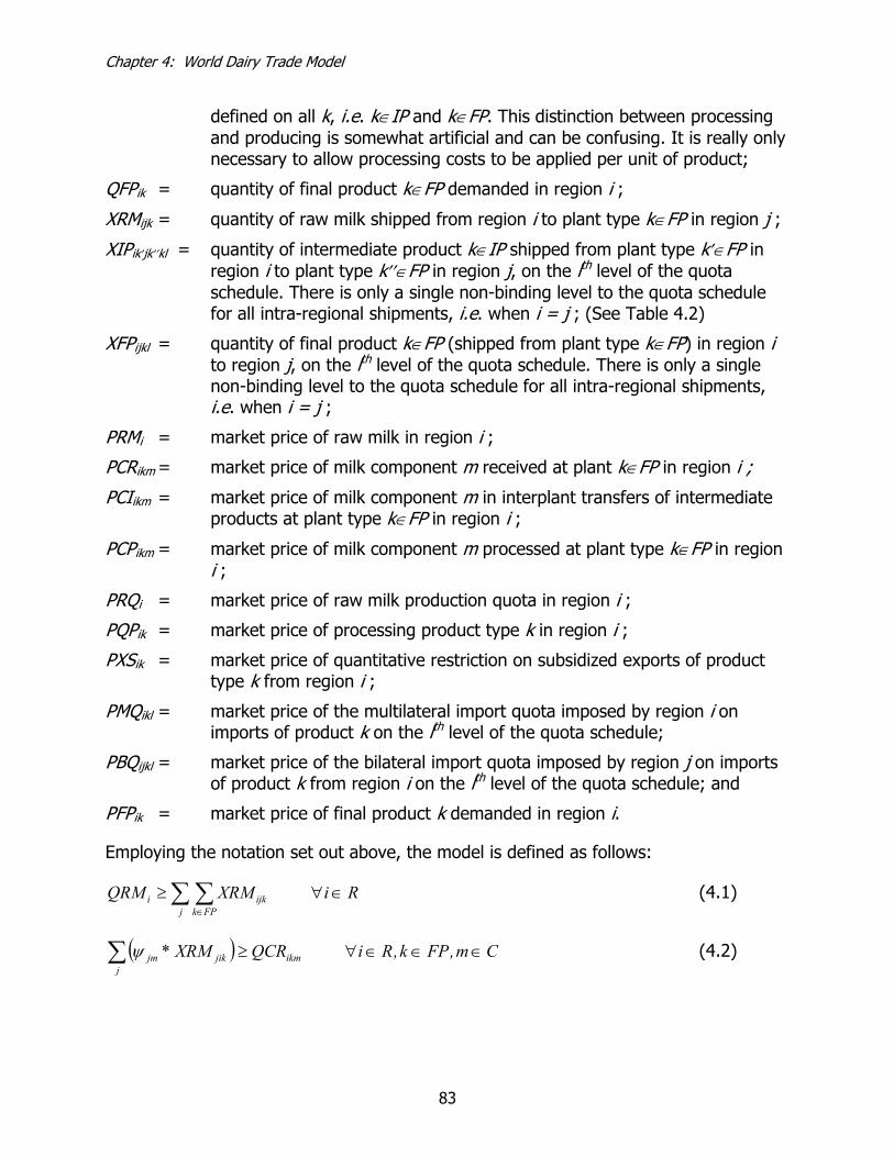
Chapter 4: World Dairy Trade Model
83
defined on all k, i.e. k∈IP and k∈FP. This distinction between processing and producing is somewhat artificial and can be confusing. It is really only necessary to allow processing costs to be applied per unit of product;
QFPik = quantity of final product k∈FP demanded in region i ;
XRMijk = quantity of raw milk shipped from region i to plant type k∈FP in region j ;
XIPik′jk′′kl = quantity of intermediate product k∈IP shipped from plant type k′∈FP in region i to plant type k′′∈FP in region j, on the lth level of the quota schedule. There is only a single non-binding level to the quota schedule for all intra-regional shipments, i.e. when i = j ; (See Table 4.2)
XFPijkl = quantity of final product k∈FP (shipped from plant type k∈FP) in region i to region j, on the lth level of the quota schedule. There is only a single non-binding level to the quota schedule for all intra-regional shipments, i.e. when i = j ;
PRMi = market price of raw milk in region i ;
PCRikm = market price of milk component m received at plant k∈FP in region i ;
PCIikm = market price of milk component m in interplant transfers of intermediate products at plant type k∈FP in region i ;
PCPikm = market price of milk component m processed at plant type k∈FP in region i ;
PRQi = market price of raw milk production quota in region i ;
PQPik = market price of processing product type k in region i ;
PXSik = market price of quantitative restriction on subsidized exports of product type k from region i ;
PMQikl = market price of the multilateral import quota imposed by region i on imports of product k on the lth level of the quota schedule;
PBQijkl = market price of the bilateral import quota imposed by region j on imports of product k from region i on the lth level of the quota schedule; and
PFPik = market price of final product k demanded in region i.
Employing the notation set out above, the model is defined as follows:
RiXRMQRMj FPk
ijki ∈∀≥ ∑ ∑∈
(4.1)
( ) Cm,FPk,RiQCRXRM*j
ikmjikjm ∈∈∈∀≥∑ ψ (4.2)

Chapter 4: World Dairy Trade Model
84
( )
( ) Cm,FPk,RiQCP*XIPδ
XIP*QCR
mkij FPk IPk l
klkikjkm
j FPk IPk lklkikjkmmki
∈∈∈∀+
≥+
′∈′′ ∈
′′′
∈′′ ∈′′′′
∑ ∑ ∑∑
∑ ∑ ∑∑
δ (4.3)
( ) Cm,FPk,RiXFP*QCPj l
ijkljkmikm ∈∈∈∀≥ ∑∑ γ (4.4)
Pk,RiXFPXIPQPPj l
ijklj FPk FPk l
klkjkiik ∈∈∀+≥ ∑∑∑ ∑ ∑ ∑∈′ ∈′′
′′′ (4.5)
FPk,RjQFPXFP jki l
ijkl ∈∈∀≥∑∑ (4.6)
RiQRMrq ii ∈∀≥ (4.7)
PkRiXFPXIPsvji l
ijklji FPk FPk l
klkjkiik ∈∀∈∀+≥ ∑∑∑ ∑ ∑ ∑≠≠ ∈′ ∈′′
′′′ , (4.8)
Ll,Pk,RjiXFPXIPmqi
ijkli FPk FPk
klkjkijkl ∈∈∀∈≠∀+≥ ∑∑ ∑ ∑∈′ ∈′′
′′′ (4.9)
Ll,Pk,RjiXFPXIPbq ijklFPk FPk
klkjkiijkl ∈∈∀∈≠∀+≥ ∑ ∑∈′ ∈′′
′′′ (4.10)
( ) RiPRMPRQQRM* iiiii
i∈∀≥+
11 εεα (4.11)
( ) FPk,Rj,iPCR*tcrPRMm
jkmimiji ∈∈∀≥+ ∑ ψ (4.12)
Cm,FPk,RiPCIPCR ikmikm ∈∈∈∀≥ (4.13)
( ) ( )
( ) Ll,FPk,Rj,iPCI*PBQPMQ
PXSts*tcPQPPCI*
mmkjkmijkljkli
jkiijklijkijklijkikm
mkikm
∈∈∈∀≥+
+++−+
++
∑
∑
′′≠
≠′
1
δ
τδ (4.14)
Cm,FPk,RiPCPPCI ikmikm ∈∈∈∀≥ (4.15)
Pk,RiPQPpc ikik ∈∈∀≥ (4.16)
( ) ( )Ll,FPk,Rj,iPFPPBQPMQ
PXSts*tcPQPPCP*
jkijkljkli
jkiijklijkijklijkikm
ikmjkm
∈∈∈∀≥+
+++−+
++
≠
≠∑
1 τγ (4.17)

Chapter 4: World Dairy Trade Model
85
( ) FPk,RiQFP*PFP ikik
ik ikik ∈∈∀≥ 1
1 ηηβ (4.18)
In order to exploit complementary slackness when solving the model, it is necessary to associate each equation with its complementary variable. The complementarity pairings are defined as in Table 4.3.
Figure 4.1. Simplified Conceptual Representation of the World Dairy Trade Model
Component balance
Consumers
Non-dairyindustry
Butter
Cheese
wmp
Price supports
Raw milk
Supply sector Processing sector Demand sector
Component balance
Consumers
Non-dairyindustry
Butter
Cheese
wmp
Price supports
Raw milk
Region 1
Region 2
IntermediateProduct Trade
TariffsQuotas (TROs)Exports subsidies
Supplyquotas
Supplyquotas
Final product trade

Chapter 4: World Dairy Trade Model
86
Table 4.2: Interplant (Intermediate Product) Shipments Allowed in the World Dairy Trade Model
Intermediate product type From plant type To plant type
Skim Milk Powder (SMP)1 SMP Cheese SMP Fluid SMP Soft products
Whole Milk Powder (WMP) WMP Cheese WMP Fluid WMP Soft products
Anhydrous Milk Fat (AMF) Butter Fluid Butter Soft products Cream Fluid Butter Fluid WMP SMP Butter SMP WMP WMP Butter
Skim milk Casein Cheese Casein Fluid Casein Soft products Casein SMP Butter Casein Butter Cheese Butter Fluid Butter Soft products Butter SMP WMP Casein WMP Cheese WMP Fluid WMP Soft products WMP SMP
Butter milk Butter Soft products Butter WMP 1 The intermediate product skim milk powder, for example, can flow from a skim milk powder
plant to a cheese plant, a fluid plant and a soft product plant. Intermediate product anhydrous milk fat is processed in a butter plant. It can flow from a butter plant to a plant for fluids and to a soft product plant.

Chapter 4: World Dairy Trade Model
87
Table 4.3. Complementary (Equation-Variable) Pairings in the World Dairy Trade Model
Equation Variable Equation Variable
(1) PRM (11) QRM
(2) PCR (12) XRM
(3) PCI (13) QCR
(4) PCP (14) XIP
(5) PQP (15) QCP
(6) PFP (16) QPP
(7) PRQ (17) XFP
(8) PXS (18) QFP
(9) PMQ
(10) PBQ
Equations (4.1) through (4.6) are essentially the underlying “primal” constraints. Together with an appropriate objective function, they would constitute an NLP formulation of the classic Samuelson-Takayama-Judge SPE type of model. Equations (4.7) through (4.10) are policy conditions, again, operating on the quantity or primal variables. Equations (4.10) through (4.18) are the “dual” conditions in the MCP formulation of the model. Alternatively, they can be thought of as zero profit, or arbitrage, conditions.
The raw milk supply and final product demand functions, equations (4.11) and (4.18) respectively, are inverted for convenience. In other words, the first term in (4.11) yields the supply price, while the right-hand side of (4.18) yields demand prices.
We now briefly describe each equation in turn. Equation (4.1) simply says that the quantity of raw milk produced in region i must exceed the quantity shipped to plants. While raw milk is theoretically able to cross regional boundaries, it is expensive to transport large distances, and may encounter hygiene-related barriers to trade. Equation (4.2) translates the raw milk delivered to plants into a quantity of m milk components. Even when raw milk is shipped inter-regionally, it is the composition of milk at the point of supply, and the quantity of milk shipped, which determines the quantity of each milk component received at plants. Equation (4.3) appears quite complex; it is the component balancing constraint associated with interplant shipments of intermediate products. It says that for each of the m component types in milk, the quantity received at a plant in the form of raw milk, plus the quantity received in the form of interplant shipments, must be greater than or equal to the quantity shipped out as interplant shipments, plus the quantity processed into final products. Equation (4.4) is another balancing constraint. It ensures that the quantity of each milk component

Chapter 4: World Dairy Trade Model
88
shipped out of a plant in the form of final products does not exceed the quantity actually processed at that plant. Equation (4.5) is included in the model for convenience; it allows us to compute the variable QPP so that we can assign processing costs on a per unit of product (final or intermediate) basis, rather than trying to estimate such costs on a component basis. Equation (4.6) simply says that the quantity of final product demanded in a region can be no more than the quantity shipped to that region (including from itself).
Equation (4.7) imposes raw milk supply quotas where they exist; equation (4.8) imposes quantitative restrictions on subsidized exports; and equations (4.9) and (4.10) impose, respectively, multilateral and bilateral import quotas. As already alluded to, the import quota schedule can have many levels or steps to it. The sum of all bilateral import quotas that any region may impose is, by definition, less than or equal to (usually less than) that region’s multilateral import quota. Incidentally, the tariffs associated with each step of the tariff-rate quota schedule must be monotonically increasing.
Equation (4.11) states that for each region, the raw milk supply price plus the raw milk supply quota value must be greater than or equal to the market price of raw milk. Equation (4.12) says that the market price of raw milk plus the cost of shipping milk to a plant must be at least as great as the price of milk at the plant. The plant price of milk is computed from the sum of the component values each multiplied by their respective composition parameters. Equation (4.13) requires that the price of a milk component, m, at the point of receipt at a plant is equal to or greater than its price when transferred elsewhere as an intermediate product shipment. Equations (4.14) and (4.17) are similar; (4.14) is the zero profit condition for intermediate products while (4.17) is the same condition for final products. Essentially, they specify the wedges that exist between prices at plants and/or plants and demand markets in terms of import tariffs (ad valorem and specific), export subsidies, transportation costs, and quota rental values. It is these two constraints that enable discriminatory ad valorem tariffs to be modeled (τijkl is defined bilaterally). As noted earlier, this is not possible in an NLP formulation.
Like equation (4.13), (4.15) is just an accounting identity that emerges from the underlying profit maximizing behavior assumed on the part of processing firms. Equation (4.16) says that the per unit cost of processing each product type must be greater than or equal to the market price of that processing activity. Finally, equation (4.18) requires that, for each region, the market price of a final product is consistent with the quantity of that product demanded and the specified inverse demand function. Government purchase prices for specific products can be established by fixing lower bounds on the price variable PFP.
The MCP can be solved in GAMS using the PATH solver (Dirske and Ferris, 1995; Ferris and Munson, 2000), and can be more computationally efficient than optimization formulations for some problems.

Chapter 4: World Dairy Trade Model
89
Data Considerations
Although the focus of this paper is on the mathematical structure of the model, a brief discussion of data is relevant. The data requirements of our model present a significant challenge due to the high degree of disaggregation in product, spatial, and policy dimensions. These data and potential sources are summarized in Table 4.4. The data required can be categorized as economic parameters, technical parameters, and policy or institutional parameters. Secondary sources can be used to obtain many of these parameters, although in some cases available data must be used to develop estimates of the necessary coefficients. Key sources for the required information are appropriate country-level agencies and the relevant literature. International agencies that collate data are also sources, e.g., WTO and APEC. As a last resort, the popular sources such as FAO and OECD can be used. Despite the challenges, Nicholson (1996) has shown the feasibility of collecting and assessing the detailed information on dairy production, processing, and consumption required for a model of the type proposed.
Concluding Comments
The world dairy industry currently faces major domestic and trade policy reform and technological changes that have the potential to markedly alter existing dairy trade patterns. To adequately analyze this potential, current dairy trade models must be modified to incorporate additional essential characteristics of the industry. This chapter has described the mathematical structure of a mixed complementarity formulation that includes many of these essential characteristics, demonstrating the potential of a MCP to extend product-specific dairy trade modeling in relevant directions.

Chapter 4: World Dairy Trade Model
90
Table 4.4. Data Requirements for the World Dairy Trade Model
Type of data Examples Sources Economic parameters Supply elasticities Raw milk, inputs (grain) and
complementary outputs (sheep, beef)
Existing estimates (e.g., SWOPSIM, FAO), academic and government literature in each region
Demand elasticities Final products, income Existing estimates (e.g., SWOPSIM, FAO), academic and government literature in each region
Price-quantity pairs in base period Raw milk and final products FAO, national statistics, EU Commission, ABARE
Transformation costs Processing costs for intermediate and final products
Academic, government, and industry sources in each region, contacts with key dairy industry leaders
Transportation costs Milk hauling, ocean freight (refrigerated vs. non-refrigerated; container vs. pallet), land-based transportation costs for manufactured products
Key industry contacts
Technical parameters Product composition Component content of raw milk,
intermediate products, and final products
USDA, FAO and national statistics data to construct component balances for key regions; contacts with dairy industry leaders
Transformation coefficients Yield relationships in dairy processing, possibilities for interplant shipments and joint production
Same as above.
Institutional and policy parameters Tariffs Traded dairy products by region
(including discriminatory tariffs) US Department of Commerce, APEC, national agencies, fee-based sources
Quotas Traded dairy products Same as above Export subsidies Subsidized exports National and regional policy
documents Levels of domestic price and quantity-related policy instruments
Support prices and associated government purchases, production quotas, retail price controls
National and regional policy documents
Chapter 4: World Dairy Trade Model
91
Chapter 4 References
Baker, A.D. 1991. An Investigation of the Dairy Subsector Impacts of a Free Trade Agreement Between Canada and the United States. Unpublished Ph.D. Dissertation, The Pennsylvania State University, University Park, Pennsylvania.
Bishop, P.M., J.E. Pratt, and A.M. Novakovic. 1993. Using a Joint-Input, Multi-Product Formulation to Improve Spatial Price Equilibrium Models. SP 94-06, Department of Agricultural, Resource, and Managerial Economics, Cornell University, 1994. Presented at the “New Dimensions in North American-European Agricultural Trade Relations” conference, Calabria, Italy, June 20-23, 1993.
Cox, T.L. and Y. Zhu. 1997. Assessing the Impacts of Liberalization in World Dairy Trade. No. 406 Agricultural and Applied Economics Staff Paper Series, University of Wisconsin, Madison, January.
Dirske, S.P. and M.C. Ferris. 1995. “The PATH Solver: A Non-Monotone Stabilization Scheme for Mixed Complementarity Problems.” Optimization Methods and Software 5:123-159.
Ferris M. C. and J. S. Pang. 1995. Engineering and Economic Applications of Complementarity Problems. MP-TR-95-07, Computer Sciences Department, University of Wisconsin, Madison, May.
Ferris, M. C., and T. S. Munson. 2000. GAMS/PATH User Guide, Version 4.3 GAMS Development Corporation.
Harrison, G. W., T. F. Rutherford, and D. Tarr. 1997. Quantifying the Uruguay Round. The Economic Journal, 107:1405-1430.
Hashimoto, H. 1984. “A Spatial Nash Equilibrium Model,” in Spatial Price Equilibrium: Advances in Theory, Computation, and Application, P.T. Harker (editor), Springer–Verlag.
Kolstad, C.D. and A.E. Burris. 1986. “Imperfectly Competitive Equilibria in International Commodity Markets,” American Journal of Agricultural Economics, 68:27-36.
Nicholson, C. F. 1996. Economic Liberalization, Free Trade, and Structural Change: A Spatial Economic Model of Mexico’s Dairy Sector. Ph. D. dissertation, Cornell University.
Nicholson, C. F., P. M. Bishop, and A. Nagurney. 1994. Using Variational Inequalities to Solve Spatial Price Equilibrium Models with Ad Valorem Tariffs and Activity Analysis. Department of Agricultural, Resource, and Managerial Economics, Cornell University, 1994. [Working Paper 94-14]
Organization for Economic Cooperation and Development (OECD). 1991. Changes in Cereals and Dairy Policies in OECD Countries: A Model-Based Analysis. OECD, Paris.
Rizvi, S. S. H. 1987. Supercritical Fluid Extraction of Dairy Foods. New York Food and Life Sciences Quarterly, 17:23–26.

Chapter 4: World Dairy Trade Model
92
Rizvi, S. S. H., and A. R. Bhaskar. 1995. Supercritical Fluid Processing of Milk Fat: Fractionation, Scale-up, and Economics. Food Technology, 49:90-97,100.
Samuelson, P.A. 1952. “Spatial Price Equilibrium and Linear Programming.” American Economic Review, 42:283–303.
Maeda, K., N. Suzuki, and H. M. Kaiser. 2001. A Economic Evaluation of the New Agricultural Trade Negotiations: A Nonlinear Imperfectly Competitive Spatial Equilibrium Approach. Department of Applied Economics and Management, Cornell University, August. [Working Paper 2001-14]
Takayama, T. and G.G. Judge. 1964. “An Interregional Activity Analysis Model of the Agricultural Sector.” Journal of Farm Economics, 46:349–365.
van Schagen, M. 2000. Impacts of Trade Liberalisation on World Dairy Markets. M. S. Thesis, Department of Agricultural Economics and Policy, Wageningen University, The Netherlands.
Chapter 5: Impacts of MPC Imports
93
Chapter 5: Market Impacts of Milk Protein Concentrate Imports
Background
As noted in Chapter 2 (p. 38) imports of milk protein concentrates (MPC) grew rapidly between 1995 and 2000. The term MPC is applied to a variety of products, but it is appropriate to distinguish between products produced by ultra-filtration and “dry blends” of powdered milk products made without ultra-filtration. Ultra-filtration is used in processing typical MPCs, but there has been a high degree of concern about the use of dry blends to circumvent US tariffs on NDM. In the Harmonized Tariff Schedule (HTS), the key US trade policy document, two types of MPCs are identified. The first includes any complete milk protein that is more than 40% milk protein by weight. These lower-protein MPCs are listed in Chapter 4 of the HTS. The second includes concentrates consisting of greater than 90% casein, and are specified in Chapter 35 of the HTS. The most rapid growth has occurred for MPCs with the lower protein content. MPC imports are important because they illustrate the dynamic consequences of US commitments to no new trade barriers under the URA. The impact of MPC imports on US milk prices also has not been fully evaluated to date. One objective of this chapter is to describe a quantitative model of the US dairy industry that includes trade linkages. This model includes sufficient product-level detail (including inter-plant shipments from one dairy product plant to another) to allow reasonable assessment of alternative policies for the milk protein product complex. Our working hypothesis is that MPC imports do not simply substitute for NDM in various product uses. Hence, there may be market impacts from reallocation of other dairy components (fat, other non-protein solids) as a result of changes in trade policy for dairy proteins. A second objective is to assess the impacts of the “Chapter 4” MPC imports on US dairy markets, including effects on farm milk prices, milk production, product prices, and government purchases of NDM. Subsequent research will assess a broader range of issues related to trade in milk protein products, including impacts of other milk protein products (e.g., casein), assessment of the market impacts of proposed legislation to limit milk protein imports, and evaluation of proposals to subsidize domestic production of casein and MPCs.
A Mixed Complementarity Model of the US Dairy Industry with Trade
Chapters 3 and 4 describe the basic nature of the Mixed Complementarity Problem (MCP) and its application to the analysis of dairy markets. The model developed in this chapter is an empirical model, rather than conceptual or theoretical. As Bishop et al. (1994) noted, the joint-input, multiple-product nature of dairy processing implies that component disaggregation is a necessary element of dairy-related SPE modeling. Previous model formulations (e.g., Pratt et al., 1997) and elsewhere in the literature have employed component balance constraints (mass-balance constraints on individual components of milk such as fat, protein, other solids) and a fixed-proportions production technology (e.g., 100 lbs of cheddar cheese requires a minimum of 33.14 lbs of fat). A related issue is the level of spatial aggregation at which component balance

Chapter 5: Impacts of MPC Imports
94
is required: at a “processing plant” level or a “regional” level. Many dairy products (e.g., nonfat dry milk) are used primarily as intermediate products in other dairy processing activities. The use of nonfat dry milk and milk protein concentrates in cheese manufacturing is an example. Models that require component balancing only within a region typically ignore the importance of intermediate products used in other dairy processing, and may overstate the flexibility of component uses because all of the milk components produced in a region can be allocated among dairy products without regard to the constraints on intermediate product form and movement that would exist in real-world processing settings. However, the empirical importance of plant versus regional component balancing has not been fully explored.
In contrast, the current model employs nonlinear yield functions to represent production rather than fixed proportion functions (as in Pratt et al., 1997), requires component balancing at the processing plant level in each region, and explicitly incorporates the use of intermediate products. Raw milk with a known composition is shipped to plants. The milk is then separated into cream and skim, each of a known (pre-determined) fat content and an endogenously determined solids-not-fat (SNF) content. In other words, the SNF content of skim and cream is dependent on the composition of the raw milk, the fat content of the skim milk and cream, and the quantity of skim and cream produced. Because the quantity of skim and cream is determined by the model, i.e., it is endogenous, it is not possible to pre-determine the SNF composition. We assume a standard ratio of protein and other nonfat solids in the SNF portion of milk. Thus, the model uses three components to represent raw milk, intermediate products, and final products.
The cream and skim is then used in one of three ways at each plant: 1) shipped as is between plants; 2) used to produce additional intermediate products which may be shipped between plants, or 3) used by itself, recombined in varying proportions, or combined with other intermediate products to produce final products. Like the cream and skim, other intermediate products and final products thus end up with an endogenously determined composition. The endogenous determination of product compositions that is made possible by the use of yield functions (i.e. product production functions) permits the balancing of all milk components supplied with all milk components used, whether the component supply is from raw milk or from imported products. In addition to raw milk, there are 20 dairy products included in the model.
Other key model characteristics include:
• 15 final products (including separate casein, caseinates, Chapter 4 MPC and Chapter 35 MPC; Table 5.1)
• 7 intermediate (inter-plant) products (NDM, cream, skim, ice cream mix, fluid whey, buttermilk, MPC > 40%; Table 5.1)
• Imports of 12 products (including separate casein, caseinates, Chapter 4 MPC and Chapter 35 MPC; Table 5.1)

Chapter 5: Impacts of MPC Imports
95
• 2 regions (California and rest of US—the latter assumed to be under FMMO regulation)
• Model base year is 2001. 2001 was a relatively high milk price year. Shifts of supply and demand curves by relevant amounts can be used to examine impacts under alternative market conditions, like the low milk price year 2002.
• Milk supply and dairy product demand elasticities are adapted from FAPRI as reported in GAO (2001).
• FMMO and California product-based pricing formulas are explicitly included, as are the purchase prices under the Dairy Price Support Program. The payments under the MILC program are also included, but were not in effect during the 2001 base year, so are not included in the base scenario discussed subsequently.
• Imports and import supply prices are endogenous, but are based on 2001 mean import values from Census Bureau import data.
• Trade policies include specific and ad valorem tariffs, TRQ and US export subsidies.
The model consists of a square system of 888 inequalities and equalities (i.e. there are 888 equations and 888 variables). The Appendix describes the model equations in detail.
Model Data
Data for the model include milk production and component composition, dairy product demand and minimum component composition, component retention factors, supply and demand elasticities, and US trade policy parameters (TRQ levels, ad valorem tariffs, unit tariffs, unit export subsidies, and limits on export subsidies). Value-based data include estimated costs of dairy product processing and distribution, milk prices, domestic dairy product prices, and imported dairy product prices. These data come from government agencies (Federal Milk Marketing Orders, NASS, California Department of Food and Agriculture), previous research (for elasticity values and processing and distribution costs), and internal model calibration runs. The data used in the base model scenario are summarized in Tables 5.2 through 5.13, with footnotes to explain data sources and calculations.

Chapter 5: Impacts of MPC Imports
96
Table 5.1 Dairy Product Designations in the US Dairy Policy Model
Product Type in Model: Product Description
Inter-mediate Final Import Export
Fluid milk (Other US only) Y
High solids fluid milk (California only) Y
Ice cream Y Y Y
Yogurt Y
Cottage cheese Y
Cheddar cheese Y Y Y
Other cheese Y Y Y
Dry whey products Y Y Y
Butter Y Y Y
Nonfat dry milk Y Y Y Y
Evaporated, condensed and dry products Y Y Y
Casein (HS 3501.10.50) Y Y
Caseinate (HS 3501.90.60) Y Y
MPC > 90% protein (HTS 3501.10.10)1 Y Y
MPC > 40% protein (HTS 0404.90.10)1 Y Y Y
40% fat cream Y
Skim milk Y
Ice cream mix Y
Fluid whey Y
Buttermilk Y
1 HTS stands for Harmonized Tariff Schedule. The numbers indicate the 8-digit product code for milk protein concentrates with greater than 90% protein, described in Chapter 35 of the HTS, and greater than 40% (but less than 90%), described in Chapter 4 of the HTS
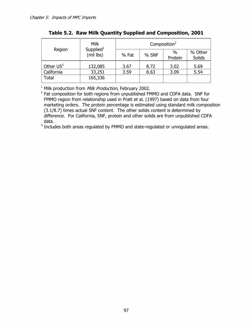
Chapter 5: Impacts of MPC Imports
97
Table 5.2. Raw Milk Quantity Supplied and Composition, 2001
Composition2 Region
Milk Supplied1 (mil lbs) % Fat % SNF %
Protein % Other Solids
Other US3 132,085 3.67 8.72 3.02 5.69 California 33,251 3.59 8.63 3.09 5.54 Total 165,336
1 Milk production from Milk Production, February 2002. 2 Fat composition for both regions from unpublished FMMO and CDFA data. SNF for
FMMO region from relationship used in Pratt et al. (1997) based on data from four marketing orders. The protein percentage is estimated using standard milk composition (3.1/8.7) times actual SNF content. The other solids content is determined by difference. For California, SNF, protein and other solids are from unpublished CDFA data.
3 Includes both areas regulated by FMMO and state-regulated or unregulated areas.

Chapter 5: Impacts of MPC Imports
98
Table 5.3. Regional Final Product Demand Estimates, Exports and Imports, 2001
Regional Final Demand1, mil lbs Product
Other US CAL
Exports, mil lbs
Imports, mil lbs
Fluid milk 49,679.7 6,424.9 0.0 0.0Ice cream 5,572.8 773.9 93.5 14.5Yogurt 1,731.0 240.4 5.3 5.9Cottage cheese 1,222.0 169.7 0.0 0.0Cheddar cheese 3,294.0 554.8 69.3 70.0Other cheese 3,868.3 530.9 45.5 143.8Whey products2 4,190.2 749.6 656.3 57.1Butter 1,171.2 187.1 3.7 45.5Nonfat dry milk 340.4 37.3 212.0 7.4Evaporated, Condensed, or Dry 704.2 102.3 125.1 37.2Casein 119.2 16.6 0.0 135.8Caseinates 74.0 10.3 0.0 84.3MPC > 90% (Chapter 35 HTS) 13.4 1.9 0.0 15.3MPC > 40% (Chapter 4 HTS) 55.1 7.7 0.0 62.8
1 Demand for fluid milk based on FMMO and CDFA data on fluid milk sales. Demand estimates for ice cream, yogurt, and cottage cheese are based on production data from Dairy Products. For other domestically produced products, data on production, change in stocks, imports, exports and dairy industry (intermediate product) use were used to develop initial demand estimates. In order to ensure component balance in the base model scenario, assumptions regarding the percentage of production covered in NASS Dairy Product surveys and intermediate product use were modified through iteration of the model structure. Demand for casein, caseinates and MPCs is based on import data. Aggregate US data for products other than fluid milk was allocated to regions based on adjusted per capita consumption (for methods, see Pratt et al., 1997) and regional population. Intermediate demands are endogenous to the model. They are not specified as explicit demand relationships, and therefore are not reported herein.
2 Final demand for whey products assumes all fluid whey is processed into dry product, which is not in fact the case. This assumption is necessary because the model does not explicitly model the costs of alternative whey disposal (other than drying). Use of actual estimated whey final product demand would result in a dry whey price of zero.

Chapter 5: Impacts of MPC Imports
99
Table 5.4. Composition of Intermediate Products from US Plants
Composition1 Product
% Fat % SNF % Protein
% Other Solids
Skim milk Other US 0.07 9.05 3.23 5.83 California 0.07 8.95 3.19 5.76
Cream Other US 40.00 5.36 1.91 3.45 California 40.00 5.30 1.89 3.41
NDM Other US 0.80 95.20 33.92 61.28 California 0.79 95.21 33.93 61.29
Ice cream mix Other US 9.17 9.74 3.47 6.27 California 9.17 9.74 3.47 6.27
Buttermilk Other US 0.77 8.99 3.20 5.79 California 0.77 9.09 3.24 5.85
MPC > 40% (Chapter 4) Other US 1.20 94.80 56.00 38.80 California 1.20 94.80 56.00 38.80
1 Fat and SNF values calculated based on raw milk composition and assumptions about the fat content of cream and skim. Values of these intermediate products are exogenous. Protein values for products determined based on protein:SNF ratio in raw milk. Other solids composition equals SNF less protein. The value of protein in MPC is based on the estimated value of protein in MPC imports (that is, product composition for domestic and imported MPC > 40% is assumed to be the same; see footnote for Table 5.5 for additional explanation.)
Table 5.5. Composition of Selected Imported Products
Composition Product
% Fat % SNF % Protein
% Other Solids
Casein 1.0 93.0 92.0 1.0 Caseinates 1.0 95.0 94.0 1.0 MPC > 90% (Chapter 35 HTS) 1.0 95.0 90.0 5.0 MPC > 40% (Chapter 4 HTS) 1.0 95.0 56.0 39.0
Source: Compositions based on information in Dairy Proteins, Wisconsin Center for Dairy Research (1999) and David Barbano, Department of Food Science, Cornell University (personal communication). Protein content of MPC > 40% based on unit value of Chapter 4 HTS MPC imports in 2001 and the unit value of protein in NDM in US markets.

Chapter 5: Impacts of MPC Imports
100
Table 5.6. Minimum Component Specifications for Final Products
Composition Product
% Fat % SNF % Protein
% Other Solids
Fluid milk Other US 2.65 California 2.36 9.64
Yogurt Other US 1.55 13.50 California 1.55 13.50
Cottage cheese Other US 15.41 15.40 California 15.41 15.40
Cheddar cheese Other US 33.00 25.50 California 33.00 25.50
Other cheese Other US 24.60 22.50 California 24.60 22.50
Source: Minimum fat content for fluid milk is actual average fat content of fluid milk sales from FMMO and CDFA data. Minimum solids content for fluid milk in California is based on regulations specifying a minimum total solids content. Other measures are based on USDA (1979).

Chapter 5: Impacts of MPC Imports
101
Table 5.7. Component Retention Factors Used to Determine the Yield of Selected Products at US Plants
% Retention Product
Fat Protein Other Solids
Cheddar cheese Other US 93 75 5 California 93 75 5
Other cheese Other US 85 75 5 California 85 75 5
Butter Other US 98 California 98
Casein Other US 75 3 California 75 3
MPC > 40% (Chapter 4) Other US 50 80 2 California 50 80 2
Source: Papadatous et al., 2002.
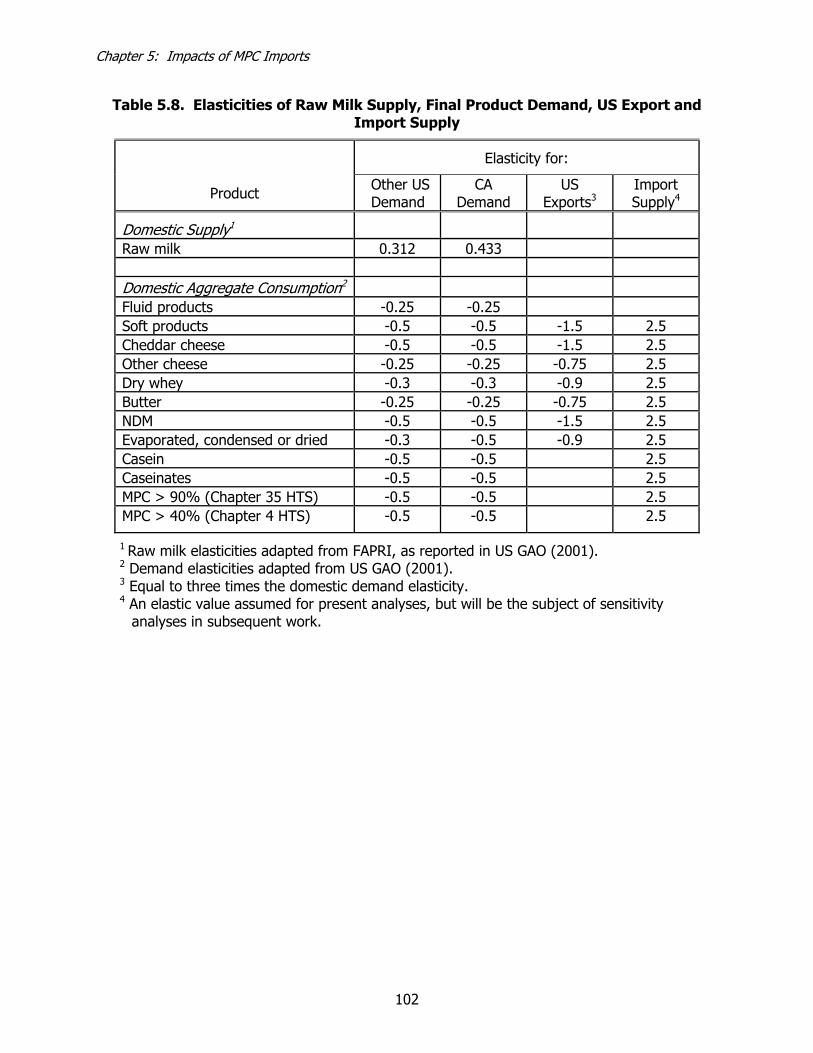
Chapter 5: Impacts of MPC Imports
102
Table 5.8. Elasticities of Raw Milk Supply, Final Product Demand, US Export and Import Supply
Elasticity for:
Product Other US Demand
CA Demand
US Exports3
Import Supply4
Domestic Supply1 Raw milk 0.312 0.433 Domestic Aggregate Consumption2 Fluid products -0.25 -0.25 Soft products -0.5 -0.5 -1.5 2.5 Cheddar cheese -0.5 -0.5 -1.5 2.5 Other cheese -0.25 -0.25 -0.75 2.5 Dry whey -0.3 -0.3 -0.9 2.5 Butter -0.25 -0.25 -0.75 2.5 NDM -0.5 -0.5 -1.5 2.5 Evaporated, condensed or dried -0.3 -0.5 -0.9 2.5 Casein -0.5 -0.5 2.5 Caseinates -0.5 -0.5 2.5 MPC > 90% (Chapter 35 HTS) -0.5 -0.5 2.5 MPC > 40% (Chapter 4 HTS) -0.5 -0.5 2.5
1 Raw milk elasticities adapted from FAPRI, as reported in US GAO (2001). 2 Demand elasticities adapted from US GAO (2001). 3 Equal to three times the domestic demand elasticity. 4 An elastic value assumed for present analyses, but will be the subject of sensitivity
analyses in subsequent work.

Chapter 5: Impacts of MPC Imports
103
Table 5.9. US Quota Levels, Ad Valorem Tariffs, Unit Tariffs, Unit Export Subsidy and Export Subsidy Quantity Limitations
Product TRQ Ad Valorem Tariff Unit Tariff Export Subsidy
Product Within Within Over Within Over Unit Subsidy
Subsidy Quantity
Mil lbs % % ¢/lb ¢/lb ¢/lb Mil lbs
Fluid products No limit 0.0 0.0 0.00 0.00 0.00 0.0 Ice cream 14.5 20.0 17.0 0.00 22.77 0.00 0.0 Yogurt No limit 0.0 0.0 0.00 0.00 0.00 0.0 Cheddar cheese 37.0 11.6 0.0 0.00 48.18 54.43 6.7 Other cheese 251.7 9.6 0.0 0.00 98.39 0.00 0.0 Dry whey No limit 7.7 0.0 0.00 0.00 0.00 0.0 Butter 15.4 0.0 0.0 5.58 69.90 81.47 46.5 NDM 11.6 0.0 0.0 1.50 39.24 54.85 212.0 ECD 22.4 0.0 0.0 1.25 7.61 0.00 0.0 Casein No limit 0.0 0.0 0.00 0.00 0.00 0.0 Caseinates No limit 0.0 0.0 0.00 0.00 0.00 0.0 MPC > 90% (Chapter 35 HTS) No limit 0.0 0.0 0.00 0.00 0.00 0.00 MPC > 40% (Chapter 4 HTS) No limit 0.0 0.0 0.00 0.00 0.00 0.00
Source: Values for TRQs and tariffs adapted from Harmonized Tariff Schedule of the United States (2001) (Rev. 1) as appropriate for model product categories. Export subsidy information from Foreign Agricultural Service, USDA.
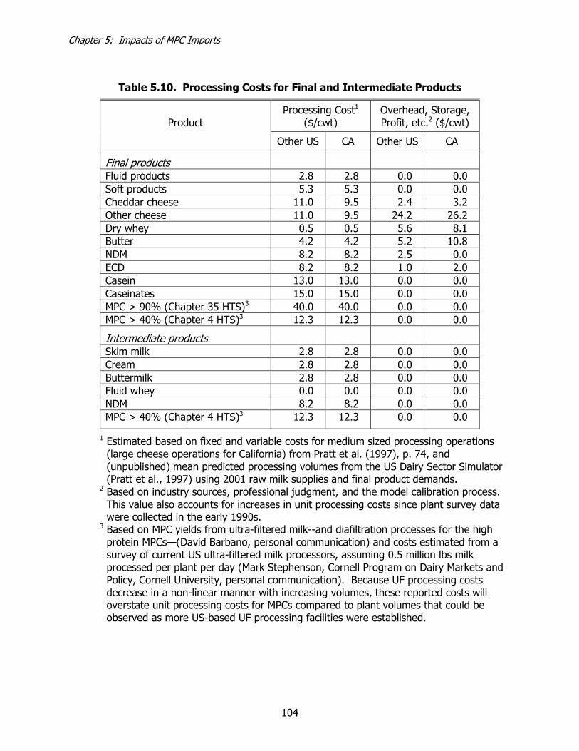
Chapter 5: Impacts of MPC Imports
104
Table 5.10. Processing Costs for Final and Intermediate Products
Product Processing Cost1
($/cwt) Overhead, Storage, Profit, etc.2 ($/cwt)
Other US CA Other US CA
Final products Fluid products 2.8 2.8 0.0 0.0 Soft products 5.3 5.3 0.0 0.0 Cheddar cheese 11.0 9.5 2.4 3.2 Other cheese 11.0 9.5 24.2 26.2 Dry whey 0.5 0.5 5.6 8.1 Butter 4.2 4.2 5.2 10.8 NDM 8.2 8.2 2.5 0.0 ECD 8.2 8.2 1.0 2.0 Casein 13.0 13.0 0.0 0.0 Caseinates 15.0 15.0 0.0 0.0 MPC > 90% (Chapter 35 HTS)3 40.0 40.0 0.0 0.0 MPC > 40% (Chapter 4 HTS)3 12.3 12.3 0.0 0.0
Intermediate products Skim milk 2.8 2.8 0.0 0.0 Cream 2.8 2.8 0.0 0.0 Buttermilk 2.8 2.8 0.0 0.0 Fluid whey 0.0 0.0 0.0 0.0 NDM 8.2 8.2 0.0 0.0 MPC > 40% (Chapter 4 HTS)3 12.3 12.3 0.0 0.0
1 Estimated based on fixed and variable costs for medium sized processing operations (large cheese operations for California) from Pratt et al. (1997), p. 74, and (unpublished) mean predicted processing volumes from the US Dairy Sector Simulator (Pratt et al., 1997) using 2001 raw milk supplies and final product demands.
2 Based on industry sources, professional judgment, and the model calibration process. This value also accounts for increases in unit processing costs since plant survey data were collected in the early 1990s.
3 Based on MPC yields from ultra-filtered milk--and diafiltration processes for the high protein MPCs—(David Barbano, personal communication) and costs estimated from a survey of current US ultra-filtered milk processors, assuming 0.5 million lbs milk processed per plant per day (Mark Stephenson, Cornell Program on Dairy Markets and Policy, Cornell University, personal communication). Because UF processing costs decrease in a non-linear manner with increasing volumes, these reported costs will overstate unit processing costs for MPCs compared to plant volumes that could be observed as more US-based UF processing facilities were established.

Chapter 5: Impacts of MPC Imports
105
Table 5.11. Transportation Costs for Raw Milk Assembly and Final Products Distribution
Distance pairs, miles1 Cost, $/ 100 lbs milk or product 2 Transportation type, product (plant) type US to
US US to CA
CA to US
CA to CA US to US US to CA CA to US CA to CA
Raw Milk Assembly To Fluid products 200 2,120 2,120 250 0.80 8.48 8.48 1.00 Soft products 50 2,120 2,120 50 0.20 8.48 8.48 0.20 Cheddar cheese 50 2,120 2,120 50 0.20 8.48 8.48 0.20 Other cheese 25 2,120 2,120 25 0.10 8.48 8.48 0.10 Dry whey3 NA 2,120 2,120 NA NA NA NA NA Butter 50 2,120 2,120 25 0.20 8.48 8.48 0.10 NDM 50 2,120 2,120 50 0.20 8.48 8.48 0.20 ECD 80 2,120 2,120 80 0.32 8.48 8.48 0.32 Casein 50 2,120 2,120 50 0.20 8.48 8.48 0.20 MPC > 40% (Chapter 4 HTS) 50 2,120 2,120 50 0.20 8.48 8.48 0.20 Final Product Distribution From Fluid products4 25 2,120 2,120 25 13.02 NA NA 14.58 Soft products5 75 2,120 2,120 75 87.3-114.7 94.9-122.0 93.3-120.6 88.9-116.0 Cheddar cheese 300 2,120 2,120 200 1.58 6.57 6.57 1.17 Other cheese 300 2,120 2,120 200 1.58 6.57 6.57 1.17 Dry whey 300 2,120 2,120 200 1.41 5.90 5.90 1.05 Butter 350 2,120 2,120 200 1.76 6.57 6.57 1.17 NDM 350 2,120 2,120 200 1.58 5.90 5.90 1.05 ECD 250 2,120 2,120 200 1.24 5.90 5.90 1.05 Casein 350 2,120 2,120 200 1.58 5.90 5.90 1.05 MPC > 40% (Chapter 4 HTS) 350 2,120 2,120 200 1.58 5.90 5.90 1.05 1 Based on (unpublished) mean predicted distances from US Dairy Sector Simulator (Pratt et al., 1997) using 2001 raw milk supplies and final
product demands for within-region shipments. Distances for inter-regional shipments based on distance between Los Angeles and Chicago. 2 Based on transportation cost relationships specified in Pratt et al. (1997). 3 Assembly of raw milk at whey “plants” is prohibited by setting an arbitrarily large distance for the assembly flow. 4 A retail margin of $1.10 and $1.38 per gallon is added in the Other US and California regions, respectively, to allow comparisons with retail
prices. 5 Varies by product. An estimated retail margin of between $0.87 cents and $1.15 per lb is included in the value to allow comparison with
reported retail prices.
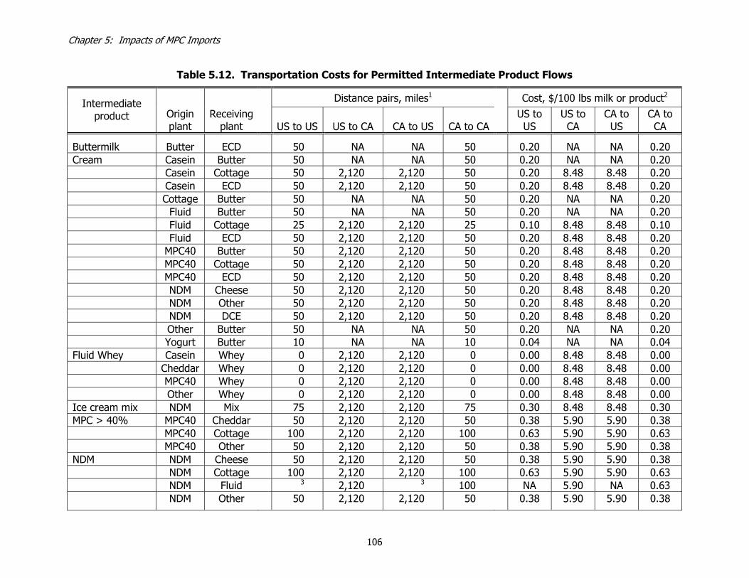
Chapter 5: Impacts of MPC Imports
106
Table 5.12. Transportation Costs for Permitted Intermediate Product Flows
Distance pairs, miles1 Cost, $/100 lbs milk or product2 Intermediate product Origin
plant Receiving
plant US to US US to CA CA to US CA to CA US to US
US to CA
CA to US
CA to CA
Buttermilk Butter ECD 50 NA NA 50 0.20 NA NA 0.20 Cream Casein Butter 50 NA NA 50 0.20 NA NA 0.20 Casein Cottage 50 2,120 2,120 50 0.20 8.48 8.48 0.20 Casein ECD 50 2,120 2,120 50 0.20 8.48 8.48 0.20 Cottage Butter 50 NA NA 50 0.20 NA NA 0.20 Fluid Butter 50 NA NA 50 0.20 NA NA 0.20 Fluid Cottage 25 2,120 2,120 25 0.10 8.48 8.48 0.10 Fluid ECD 50 2,120 2,120 50 0.20 8.48 8.48 0.20 MPC40 Butter 50 2,120 2,120 50 0.20 8.48 8.48 0.20 MPC40 Cottage 50 2,120 2,120 50 0.20 8.48 8.48 0.20 MPC40 ECD 50 2,120 2,120 50 0.20 8.48 8.48 0.20 NDM Cheese 50 2,120 2,120 50 0.20 8.48 8.48 0.20 NDM Other 50 2,120 2,120 50 0.20 8.48 8.48 0.20 NDM DCE 50 2,120 2,120 50 0.20 8.48 8.48 0.20 Other Butter 50 NA NA 50 0.20 NA NA 0.20 Yogurt Butter 10 NA NA 10 0.04 NA NA 0.04 Fluid Whey Casein Whey 0 2,120 2,120 0 0.00 8.48 8.48 0.00 Cheddar Whey 0 2,120 2,120 0 0.00 8.48 8.48 0.00 MPC40 Whey 0 2,120 2,120 0 0.00 8.48 8.48 0.00 Other Whey 0 2,120 2,120 0 0.00 8.48 8.48 0.00 Ice cream mix NDM Mix 75 2,120 2,120 75 0.30 8.48 8.48 0.30 MPC > 40% MPC40 Cheddar 50 2,120 2,120 50 0.38 5.90 5.90 0.38 MPC40 Cottage 100 2,120 2,120 100 0.63 5.90 5.90 0.63 MPC40 Other 50 2,120 2,120 50 0.38 5.90 5.90 0.38 NDM NDM Cheese 50 2,120 2,120 50 0.38 5.90 5.90 0.38 NDM Cottage 100 2,120 2,120 100 0.63 5.90 5.90 0.63 NDM Fluid 3 2,120 3 100 NA 5.90 NA 0.63 NDM Other 50 2,120 2,120 50 0.38 5.90 5.90 0.38

Chapter 5: Impacts of MPC Imports
107
Distance pairs, miles1 Cost, $/100 lbs milk or product2 Intermediate product Origin
plant Receiving
plant US to US US to CA CA to US CA to CA US to US
US to CA
CA to US
CA to CA
Skim Casein Cheese 75 2,120 2,120 75 0.30 8.48 8.48 0.30 Casein Cottage 75 2,120 2,120 75 0.30 8.48 8.48 0.30 Casein ECD 75 2,120 2,120 75 0.30 8.48 8.48 0.30 Casein Other 75 2,120 2,120 75 0.30 8.48 8.48 0.30 MPC40 Cheese 75 2,120 2,120 75 0.30 8.48 8.48 0.30 MPC40 Cottage 75 2,120 2,120 75 0.30 8.48 8.48 0.30 MPC40 ECD 75 2,120 2,120 75 0.30 8.48 8.48 0.30 MPC40 Other 75 2,120 2,120 75 0.30 8.48 8.48 0.30 NDM Cheese 75 2,120 2,120 75 0.30 8.48 8.48 0.30 NDM Cottage 75 2,120 2,120 75 0.30 8.48 8.48 0.30 NDM ECD 75 2,120 2,120 75 0.30 8.48 8.48 0.30 NDM Other 75 2,120 2,120 75 0.30 8.48 8.48 0.30
1 Based on (unpublished) mean predicted distances from U. S. Dairy Sector Simulator (Pratt et al., 1997) using 2001 raw milk supplies and final product demands for within-region shipments. Distances for inter-regional shipments based on distance between Los Angeles and Chicago.
2 Based on transportation cost relationships specified in Pratt et al. (1997). 3 Use of NDM in fluid milk is not allowed in the FMMO region. It is allowed in California due to the higher solids requirement for fluid
milk products.

Chapter 5: Impacts of MPC Imports
108
Table 5.13. Milk Supply, Regional Demand, Import Supply and Export Demand Prices and Data Sources
Reference Price ($/cwt)
Product Other US CA Import Supply1
Export Demand1 Definition and Sources (US Values)
Supply
Raw milk 15.23 13.72 NA NA
FMMO = [US mean annual all-milk price – (CA mean annual all-milk price)(Proportion US milk production in California)]/Proportion US milk in FMMO region. CA=mean annual all-milk price. Agricultural Prices, various issues 2001-2002
Final demand
Fluid products2 32.00 33.00 NA NA FMMO = US city annual average of whole and lowfat gallon milk prices. CA=annual average of west urban whole milk prices. Bureau of Labor Statistics (BLS)
Ice cream 148.00 148.00 148.00 35.00 US city annual average of ice cream price reported by BLS. Yogurt 129.00 129.00 135.00 33.00 US city annual average of yogurt price reported by BLS.
Soft products 135.00 135.00 135.00 US city annual average of ice cream and yogurt prices reported by BLS.
Cheddar cheese 148.70 145.40 125.00 130.00 Annual average of weekly national 500-lb barrel prices
reported by NASS. Other cheese 148.70 145.40 125.00 130.00 Assumed equal to cheddar prices based on industry sources.
Dry whey 28.5 25.50 88.00 25.00 Annual average of weekly national prices for dry whey reported by NASS.
Butter 164.00 162.00 99.00 99.00 Annual average of weekly national prices for butter reported by NASS.
NDM 94.50 92.20 55.00 55.00 Annual average of weekly national prices for NDM reported by NASS.
ECD 40.00 40.00 30.00 30.00 Adapted from annual average of monthly prices for evaporated milk, Class II condensed skim and Class III condensed skim reported in Dairy Market News.

Chapter 5: Impacts of MPC Imports
109
Reference Price ($/cwt)
Product Other US CA Import Supply1
Export Demand1 Definition and Sources (US Values)
Casein 217.00 217.00 217.00 NA Based on unit value of imports from Customs data.
Caseinates 233.00 233.00 233.00 NA Based on unit value of imports from Customs data.
MPC > 90% 219.00 219.00 219.00 NA Based on unit value of imports from Customs data.
MPC > 40% 163.00 163.00 163.00 NA Based on unit value of imports from Customs data.
1 Based on unit value of imports from Customs data. 2 Gallon prices are $2.75 and $2.84 in the FMMO region and California, respectively.
Chapter 5: Impacts of MPC Imports
110
Results and Discussion
Scenarios Simulated
To assess the impacts of MPC imports, four scenarios are simulated and compared. The first is a base scenario, which replicates average annual market outcomes (e.g., milk production, milk and product prices) during 2001. This scenario allows MPC imports to enter the US at prices estimated from trade data complied by the Customs Bureau. The predicted outcomes of this base scenario are compared to actual market outcomes to assess how well the model replicates the base year data. The substitutability of Chapter 4 MPCs with NDM and with other non-milk (e.g., soy proteins) is important to the market outcome of MPC imports, especially when the Dairy Price Support Program is purchasing NDM. Harris (2003) and others have suggested that when the CCC is purchasing sufficiently large quantities of NDM, MPC imports have no impact on farm milk or classified prices. Rather, MPC imports only increase government NDM purchases and expenditures. However, this outcome occurs only if there is perfect substitutability between NDM and MPCs in both intermediate and final demand, and there is no substitutability between MPCs and non-milk protein sources in final demand. Because little or no information exists about the substitutability for MPCs with alternatives—which is crucially important to market outcomes of MPC imports—we simulate three alternative scenarios that will be compared to results of the base. A second scenario is similar to the base scenario, but prohibits the imports of MPCs entering under Chapter 4 of the HTS1. We assume that substitutes for MPC (such as NDM) can be found for dairy industry uses, but that there is a demand for MPCs in other uses that must be met by domestic production of MPCs. That is, the use of MPC as an “intermediate” product in the manufacture of other dairy products is endogenous and is determined by the relative prices of the substitute protein-intensive intermediate products (NDM and skim milk) generated by the model. The demand for MPCs for other food industries is assumed to sensitive to the price of MPCs, but there are no immediately available (dairy or non-dairy) substitutes. This means that there will continue to be demand for MPCs in these industries even if no imports of MPC are allowed. Thus, the price of MPCs will increase to support the level of domestic production required to service the needs of the non-dairy industry users. Because there was essentially no domestic production of MPCs in 2001, import data indicate the total amount of MPCs demanded by dairy industry and non-dairy industry users. No data are currently available to estimate the amount of MPCs used in dairy and non-dairy industry uses, although a survey of the importers and users of MPC was conducted by the US International Trade Commission in 2003. (Some of this
1 This is equivalent to setting the TRQ for imports of Chapter 4 MPCs (i.e., the parameter qlvl in equation 5.22) equal to zero.

Chapter 5: Impacts of MPC Imports
111
information may be made public in May 2004.) Thus, we must make an assumption about the division of MPC imports into “intermediate” (dairy industry) and “final” (non-dairy industry) use. For the purposes of this analysis, we assume that 30% of the 62.8 million lbs of MPC imports that entered the US in 2001 were used by the dairy industry (e.g., in manufacture of cheese without a standard of identity) and 70% of MPC imports were used for non-dairy industry manufacturing. Under the third scenario, NDM is assumed to be perfectly substitutable with Chapter 4 MPC imports at the NDM purchase price, and no imports of Chapter 4 MPCs are allowed. The import ban results in an increase in the final commercial demand for NDM for use in final products equal to the amount of NDM required to supply the milk protein assumed to enter the US in MPC imports. Thus, there is an increase in final demand for NDM of about 103 million lbs. Demand for NDM as an intermediate product remains endogenous. In the fourth scenario, there is no substitutability between Chapter 4 MPCs and NDM, but perfect substitutability between MPCs and non-milk proteins at the current MPC price. Thus, when Chapter 4 MPC imports are banned, there is no additional demand for milk protein. Instead, the final demand for Chapter 4 MPCs is assumed to be zero. Although none of the three scenarios is completely plausible, they illustrate the range of possible market impacts. The base scenario simulated by the model compares favorably to the observed market outcomes (Table 5.14). The all-milk price is within $0.02/cwt of the actual for the Other US regions, and within $0.09/cwt in California. The weighted average all-milk price for the US predicted by the model is the same as the actual. With the exception of the Class 4b price in California, all minimum class prices are within $0.01/cwt of the actual values. All product prices in both regions are within $0.02/lb of the observed market prices. Our predictions of NDM purchases by the CCC are somewhat high, about 7 million lbs, or just under 3%. Model evaluation will be discussed in further detail in subsequent publications.
Summary of Market Impacts
The simulation of a ban on MPC imports under the second scenario indicates that farm-milk price impacts are relatively modest (Table 5.14). The weighted average US all-milk price increases by $0.06/cwt, and US milk production increases 200 million lbs or 0.1%. There is a reduction in the butter price of about $0.07/lb because additional butter (21 million lbs) is manufactured as a by-product of the MPC manufacturing process2. This effect supports our initial hypothesis that there can be market impacts from reallocation of other dairy components (fat in this case) as a result of changes in trade policy for dairy protein products. (It also illustrates the need to account for joint products in the
2 Recall that the MPC manufacturing process yields cream (which can be used in the manufacture of butter as well as other products) and a lactose-rich by-product used in the “dry whey” product category.

Chapter 5: Impacts of MPC Imports
112
modeling of dairy markets). In essence, the demand for domestically produced MPCs increases the demand for domestically produced milk proteins. In order to meet this demand, increased milk production occurs in response to price shifts. Additional milk production results in additional butterfat, and the value of butterfat must fall to clear the fat market. Butter prices are used in the classified pricing formulas for all classes in both regions. The largest impact of increased butter production is on the Class IV price in the FMMO region and the Class 4a price in California. The reduction in the butter price results in a $0.29/cwt fall in the Class IV price, and a $0.28/cwt decrease in the Class 4a price. Thus, there is a negative effect on milk prices that arises from adjustments in the butterfat market in response to the reduction in milk protein imports. Cheese prices increase by 1 to 2 cents per lb as a result of both an increase in the demand for milk proteins required for MPC manufacture, and because the value of butterfat contributes negatively to the cheese price in the Class III and Class 4b pricing formulas (for a given cheese price). That is, as the butter price falls, the price of milk used in cheese will increase, ceteris paribus. However, the current pricing formulas imply that the increase in the Class III price due to a fall in the butterfat value will be less than the amount of decrease in the Class IV or 4a prices. Dried whey prices decrease about $0.01/lb, so there is a second negative effect on milk prices through the “other solids” price in classified pricing formulas. On net, however, there is an increase in the Class III and Class 4b prices of $0.16/cwt and $0.10/cwt, respectively. The all-milk price in the FMMO region increases despite the fall in the Class IV price because utilization is sufficiently larger in Class III than Class IV. In the FMMO region, the impacts on Class I and Class II mirror the impacts on the Class III and IV prices. Differences in the Class II price will be equal to those in the Class IV price, because these two prices differ by only the $0.70/cwt Class II differential. The impact on Class I depends on whether Class III or Class IV is the “higher of” price used as the base price for milk used in fluid products. In our 2001 base scenario, Class III was the “higher of”, and thus the Class I price increases by the same amount as the Class III price in response to the ban on Chapter 4 MPC imports. Production (consumption) of fluid milk decreases 113 million lbs due to increases in the Class I price resulting from the increase in the Class III price. Production of ice cream increases due to the reduction in the fat price. Total cheese production falls about 33 million lbs (0.4%) as a result of increases in the Class III price. NDM production declines 34 million lbs, or about 4.0%. As a result, CCC purchases of NDM decrease by roughly the same amount, resulting in a reduction of $32 million in government expenditures under the Dairy Price Support Program. The farm-milk price effects differ in the two regions, in both magnitude and direction. In California, the higher proportion of Class 4a utilization (28% versus 8% in the rest of the US) means that the reduction in the Class 4a price ends up having a larger effect on

Chapter 5: Impacts of MPC Imports
113
the blend price than the increase in the Class 4b price. Thus, the all-milk price in California decreases in response to the MPC import ban3, and production declines by 30 million lbs. In the rest of the US, the farm-milk price increases by about $0.08/cwt, and production increases by 230 million lbs. Although our model currently does not disaggregate the “other US” region into additional regions (FMMO marketing areas being an obvious example), it is likely that there will be similar differences among the various regions other than California. Regions with relatively greater Class III utilization are likely to see relatively larger increases in the farm-milk price. Under the third and fourth scenarios, there are no market price or production impacts (and thus the scenario results are not shown in Table 5.14). When NDM and Chapter 4 MPCs are perfect substitutes, the only difference with the base scenario is a reduction in NDM purchases under the DPSP of 103 million lbs (essentially equal to the assumed increase in commercial NDM demand) and a reduction in government expenditures of $96 million. When Chapter 4 MPCs are perfect substitutes with non-dairy proteins, the outcomes are identical to the base scenario except that MPC imports fall to zero. That is, there is no reduction in NDM purchases by the government and no decrease in government expenditures.
Conclusions and Implications
Our model of the US dairy industry suggests relatively modest farm-milk price impacts resulting from imports of lower-protein content MPCs. When MPCs are not substitutable with NDM or non-dairy protein, a ban on imports would have a small positive impact on US all-milk prices, due primarily to an increase in the domestic demand for milk protein. However, there will also be negative effects on milk prices that arise through reductions in the value of butterfat (reductions in the Class IV or 4a prices) as more milk is produced, and through reductions in the dry whey price (which offsets some of the increase in the Class III or 4b prices). The presence of these offsetting effects implies that some regions may see larger-than-average gains in farm-milk prices if MPC imports were prohibited, but that some regions (notably California with its larger Class 4a utilization) may see reductions in farm-milk prices. Importantly, our simulation results address only a small fraction of the total imports of milk protein products into the US. Imports of Chapter 4 MPCs accounted for only one-fifth of the volume of milk protein product imports in 2001, and probably substantially less than that on a protein-equivalent basis. This implies that current efforts to markedly reduce all milk protein imports (as in the legislation currently under consideration by the US Congress) or to subsidize domestic production are likely to have larger impacts on US dairy markets. The assumption of perfect substitutability between NDM or non-diary protein products and casein, caseinates and Chapter 35
3 The reduction in the all-milk price in California arises because of reductions in both the blend price and a reduction in the over-order premium estimated by the model. Each of these contributes equally to the overall reduction of $0.03/cwt.

Chapter 5: Impacts of MPC Imports
114
MPCs is much less plausible. Thus, it is highly likely that there will be impacts on US dairy market prices and production—as in our second scenario. Although it remains to be confirmed by forthcoming research, it is likely that more dramatic restrictions of milk protein imports or domestic subsidy programs will result in substantially larger positive impacts on cheese prices (and substantial increases in Class III and 4b prices; and thus Class I prices). It is also likely that there will be much larger reductions in the butter price (and Class IV and 4a prices). Unless the effects of increases in the Class III/4b price and decreases in the Class IV/4a are of similar magnitude, the potential exists for the positive and negative effects on farm milk prices to be larger if greater restrictions on milk protein imports are put in place. Further modeling of these alternative scenarios will be undertaken in the near future. The impact on class prices and farm milk prices will also differ if market conditions dictate that Class IV is the “higher of” price used to set minimum regulated prices for milk used in fluid products. The impact of restricting milk protein imports on Class I prices would be different if Class IV were the “higher of” in a base scenario. In that case, the change in the Class I price would equal the change in the Class IV price (i.e., a decrease) if Class IV was still the “higher of” in the scenario prohibiting Chapter 4 MPC imports. If the Class IV price falls below the Class III in response to prohibiting Chapter 4 MPC imports, there would likely still be a fall in the Class I price, but it would be attenuated by the use of the (now higher) Class III price as the base price for Class I. When the Class IV price is the “higher of,” it is used as the base to price milk in Classes I, II, and IV. Under this circumstance, a fall in the Class IV price will have larger impacts on farm milk prices. In general, if Class IV is the “higher of” there will be fewer positive impacts on farm milk prices (and a greater possibility of farm milk price decreases) due to the fall in the price of butter resulting from restrictions on imports of milk protein products.
Chapter 5 References
Bishop, P. M., J. E. Pratt, and A. M. Novakovic. 1994. Using a Joint-Input, Multi-Product Formulation to Improve Spatial Price Equilibrium Models. Department of Agricultural, Resource and Managerial Economics, Cornell University. [Staff Paper 94-06]
Harris, H. 2003. U. S. Dairy Programs and World Trade Policy Issues, in “Looking Ahead…or Looking Behind?” Proceedings of the 10th Annual Invitational Workshop for Dairy Economists and Policy Analysts. Memphis, TN, April 23-24, 2003. National Institute for Livestock and Dairy Policy.
Papadatous, A., A. M. Berger, J. E. Pratt, and D. M. Barbano. 2002. A Nonlinear Programming Optimization Model to Maximize Net Revenue in Cheese Manufacture. Journal of Dairy Science, 85: 2768-2785.

Chapter 5: Impacts of MPC Imports
115
Pratt, J. E., P. M. Bishop, E. E. Erba, A. M. Novakovic and M. W. Stephenson. 1997. A Description of the Methods and Data Employed in the US Dairy Sector Simulator, Version 97.3. Department of Agricultural, Resource and Managerial Economics, Cornell University. [Research Bulletin 97-09]
USDA. 1979. Conversion Factors and Weights and Measures For Agricultural Commodities and their Products. Economics, Statistics and Cooperatives Service. [Statistical Bulletin No. 616]
US General Accounting Office. 2001. Dairy Industry: Estimated Economic Impacts of Dairy Compacts. Report to the Honorable Herbert Kohl, US Senate, September.
Wisconsin Center for Dairy Research. 1999. Dairy Proteins. Report prepared for the Wisconsin Milk Marketing Board.

Chapter 5: Impacts of MPC Imports
116
Table 5.14. Summary of Estimated US Dairy Market Impacts of Chapter 4 MPC Imports1
Base Scenario with MPC Imports Scenario With No MPC2 Imports
Variable, Region or Product Reference Value Value
Difference from
Reference
% Difference
from Reference
Value Difference from Base
% Difference from Base
Raw milk supply, billion lbs California 33.251 33.34 0.09 0.3% 33.32 -0.03 -0.1%Other US 132.085 132.04 -0.04 0.0% 132.27 0.23 0.2%
All milk price, $/cwt
California 13.72 13.81 0.09 0.6% 13.78 -0.03 -0.2%Other US 15.23 15.21 -0.02 -0.1% 15.30 0.08 0.6%
Weighted Average 14.93 14.93 0.00 0.0% 14.99 0.06 0.4%
Blend Price at Standard Test, $/cwt California 13.52 13.51 -0.01 -0.1%Other US 14.56 14.64 0.08 0.5%
Minimum Class Prices at Standard Test, $/cwt3 California
Class 1 15.36 15.35 -0.01 0.0% 15.43 0.08 0.5%Class 2/3 13.84 13.84 0.00 0.0% 13.56 -0.28 -2.0%Class 4b 12.95 13.03 0.08 0.6% 13.12 0.10 0.7%Class 4a 13.09 13.09 0.00 0.0% 12.80 -0.28 -2.2%
Other US Class I 16.23 16.24 0.01 0.1% 16.41 0.16 1.0%Class II 13.93 13.93 0.00 0.0% 13.64 -0.29 -2.1%Class III 13.54 13.55 0.01 0.1% 13.72 0.16 1.2%Class IV 13.23 13.23 -0.01 0.0% 12.94 -0.29 -2.2%

Chapter 5: Impacts of MPC Imports
117
Base Scenario with MPC Imports Scenario With No MPC2 Imports
Variable, Region or Product Reference Value Value
Difference from
Reference
% Difference
from Reference
Value Difference from Base
% Difference from Base
Wholesale FOB Prices, $/lb California
Cheddar cheese 1.45 1.44 -0.01 -0.8% 1.45 0.01 0.8%Other cheese 1.45 1.46 0.01 0.6% 1.48 0.02 1.1%Whey products 0.26 0.25 -0.01 -3.1% 0.24 -0.01 -2.0%Butter 1.62 1.60 -0.02 -1.4% 1.53 -0.07 -4.3%NDM 0.92 0.93 0.01 1.2% 0.93 0.00 0.0%Evaporated, condensed, and dried 0.40 0.39 -0.01 -2.8% 0.38 -0.01 -1.8%
Other US Cheddar cheese 1.49 1.49 0.01 0.4% 1.50 0.01 0.7%Other cheese 1.49 1.49 0.00 -0.1% 1.50 0.02 1.2%Whey products 0.29 0.26 -0.02 -7.4% 0.27 0.01 3.0%Butter 1.64 1.65 0.01 0.3% 1.58 -0.07 -4.1%NDM 0.95 0.93 -0.01 -1.3% 0.93 0.00 0.0%Evaporated, condensed, and dried 0.40 0.39 -0.01 -2.8% 0.38 -0.01 -1.8%
Total US Production of Final Products, billion lbs Fluid (Other US only) 49.732 49.627 -0.105 -0.2%High-solids fluid milk (CA only) 6.423 6.415 -0.008 -0.1%Ice cream 6.443 6.463 0.020 0.3%Yogurt 1.979 1.979 0.000 0.0%Cottage cheese 1.390 1.396 0.006 0.4%Cheddar cheese 3.826 3.811 -0.015 -0.4%Other cheese 4.243 4.225 -0.018 -0.4%Whey products 5.501 5.478 -0.023 -0.4%Butter 1.317 1.338 0.021 1.6%NDM 0.844 0.810 -0.034 -4.0%Evaporated, condensed, and dried 0.859 0.867 0.008 0.9%MPC > 40% (Chapter 4 HTS) 0.000 0.044 0.044

Chapter 5: Impacts of MPC Imports
118
Base Scenario with MPC Imports Scenario With No MPC2 Imports
Variable, Region or Product Reference Value Value
Difference from
Reference
% Difference
from Reference
Value Difference from Base
% Difference from Base
CCC Product Purchases, million lbs NDM 259.9 267.1 7.2 2.8% 232.9 -34.3 -12.8%
Value of CCC Product Purchases, $ million NDM 242.6 249.3 6.7 2.8% 217.3 -32.0 -12.8%
1 Results are shown only for two of the scenarios because only government purchases of NDM and expenditures are different from the base under the third and fourth scenarios.
2 Only MPCs under Chapter 4 of the HTS are prohibited in this scenario. 3 Reference classified prices reported here are calculated using the average of weekly wholesale NASS product prices for 2001 in the
product-pricing formulas specified under FMMOs. This calculation ensures a consistency between reference product prices and reference classified prices, which is not present for the actual reported prices due to lags in the pricing formulas and use of a different wholesale price series.
Chapter 5: Impacts of MPC Imports
119
APPENDIX: Additional Discussion of Model Structure and Equations
Like the models described in the previous chapters, this model has at its core the basic characteristics of a traditional Samuelson-Takayama-Judge (SJT) price equilibrium model. That is, a solution to the model requires that prices in one market are explicitly linked to prices in another as a strict equality, provided a non-zero physical flow between the two markets exists. Conversely, the price linkage between the two markets can be expressed as a strict inequality if the physical flow is zero. In the canonical SJT model, the markets are separated by space, hence such models are known as spatial price equilibrium (SPE) models. But the separation need not be spatial; it might be the form of market levels along the value chain or product forms or time.
If a typical SJT model contains a quadratic objective function and only linear constraints, then the model will be formulated and solved as a quadratic programming (QP) problem. A model with linear supply and demand functions could be formulated as a QP problem provided all the constraints were linear. A more general nonlinear programming (NLP) formulation would be necessary if: (a) any of the constraints were nonlinear, and/or (b) the objective function was nonlinear but not quadratic. An example of an NLP formulation would be where the supply and demand functions were iso-elastic, i.e. they are curved.
Formulation of the Model
One of the key departures from the usual SJT formulation is that our model is formulated and solved as a Mixed Complementarity Problem (MCP). All NLPs can be recast as MCPs but not all MCPs can be formulated as an NLP. Hence, the MCP framework permits greater flexibility in terms of the economic structures that can be modelled. In our dairy policy model, there are three main reasons why we chose to formulate the model as an MCP:
1) The ease with which ad valorem tariffs can be incorporated, i.e. there is no need to solve a sequence of NLPs containing specific (per unit) tariffs while iterating towards the desired solution, which contains specific approximations to the underlying ad valorem tariff rate. The mathematics underlying this issue have to do with the so-called integrability problem. The integrability problem is made redundant with MCPs, and this also makes the MCP formulation well-suited to regime switching models, e.g. where a shock to the model causes the solution to switch from one regime, say, imports occurring within a quota, to another regime such as imports coming in over the quota.
2) Our dairy policy model is highly nonlinear. For example, many of the regulated pricing constraints contain nonlinearities. The presence of a high number of nonlinearities makes solving the model more difficult using NLP solvers. This comes about because NLP solvers are unable to exploit second-order information, (i.e. GAMS provides first order derivatives only to the chosen solver). An MCP is formulated in GAMS with explicit first order derivatives (that is more or less the

Chapter 5: Impacts of MPC Imports
120
definition of an MCP). Hence, GAMS then effectively provides second order derivatives to the solver. The ability to exploit this second order information greatly enhances the ability to solve the problem. In order to obtain similar outcomes from NLP solvers, it is often necessary to overly constrain the model and/or bound the variables to restrict the domain over which the model is able to locate a solution.
3) A third, albeit less compelling reason, is that the MCP solution algorithm (i.e. PATH) is more efficient because it is able to exploit the complementary structure inherent in price equilibrium models. This is perhaps less of a concern with the availability of modern inexpensive computers.
“Primal” Constraints
The MCP model can be expressed in terms of “primal” (quantity-based) constraints, “dual” (value-based) constraints, minimum classified pricing formula definitions (applicable to Federal Milk Marketing Order areas) and California-specific pricing formulas. The primal constraints are as follows: ASSEMBLY(i) Defined for all I supply regions.
∑∑∑≥j fp cl
clfpjii XRMQS ,,, (5.1 )
The quantity of raw milk supplied at region I, QS, is greater than sum of milk shipped to processing plants of type FPεP in region J. VOLMFSEP(j,fp,ip) Defined for IP=cream, skim at FP=plants that can receive raw milk (fluid, yogurt, cottage cheese, cheddar cheese, other cheese, NDM and evaporated, condensed, and dried products).
∑∑ ≥⋅i cl
ipfpjclfpjiipj QMFSEPXRMρ ,,,,,, (5.2 )
The volume of cream and skim separated at a plant receiving fluid milk, QMFSEP, is less than or equal to the amount of raw milk received at the plant times an allocation factor, ρ. The allocation factor is calculated using an independent system of simultaneous equations, solving for the volume and composition of the cream and skim fractions assuming separated cream is 40% butterfat. VOLMFUSE(j,fp,ip) Defined for IP=cream and skim at FP=plants that can receive raw milk (fluid, yogurt, cottage cheese, cheddar cheese, other cheese, NDM and evaporated, condensed, and dried products).
ipfpjMIXipNDMfpjipfpjipfpj QIPQUSEMIXQMFUSEQMFSEP ,,,,,,,, ++≥ ∈∈ (5.3 )

Chapter 5: Impacts of MPC Imports
121
where QMFUSE is the amount of cream or skim used in final products, QUSEMIX is the amount of cream or skim used in ice cream mix (at FP=NDM only) and QIP is cream or skim used in intermediate products. QIP is defined for inter-plant flows of cream from fluid, yogurt, cottage cheese, other cheese, NDM plants and inter-plant flows of skim from NDM plants. The quantity of cream and skim separated at a plant is greater than or equal to the quantity used in final products at that plant, the quantity used in ice cream mix at NDM plants, and the allowable inter-plants of cream and skim. YLDMIX(j,fp,ip) Defined for FP=NDM and IP=ice cream mix only.
NDMfpMIXipjQIP
ConcSkimjθ
OHSkimipjθSkimipNDMfpjQUSEMIXCreamipNDMfpjQUSEMIX
∈∈≥∈−⋅∈∈+∈∈
,,
/),1(,,,,2
(5.4 )
The volume of ice cream mix produced at FP=NDM is less than or equal to the volume of cream used in ice cream mix at FP=NDM and the volume of concentrated skim used in ice cream mix at FP=NDM. The volume of concentrated skim is calculated as the volume of skim used in ice cream mix times one minus the water content of skim divided by the total solids content of the concentrated skim. MIXSPEC(j,fp,ip) Defined for FP=NDM and IP=cream and skim only.
NDMfpMIXipjSkimCreamipjSkimCreamipNDMfpj QIPQUSEMIX ∈∈∈∈∈ ⋅≥ ,,,,,,, δ (5.5 )
The volume of cream and skim used in ice cream mix at FP=NDM equals a proportion δ of the volume of ice cream mix processed. The value of δ is calculated using an independent system of simultaneous equations based on the desired fat content of the ice cream mix (volume basis). YIELDV(j,fp) Defined for FP=Fluid milk, yogurt, ice cream and yogurt.
fpjQFPjj ip ql
qlfpipjjjXIPMSkimCreamip jj ip ff
fpffipjjjXIPipfpjQMFUSE
,,,,,
,,,,,,,
≥+
∈+
∑∑∑
∑ ∑∑∑ (5.6 )
The volume of final product produced at a plant, QFP, is less than or equal to the cream and skim used in final products plus the volume of interplant shipments of IP, XIP, to the plant allowed from plant type FF in region JJ, plus the volume of imported IP, XIPM, to the plant under all quota levels (ql).

Chapter 5: Impacts of MPC Imports
122
YLDCOT(j,fp) Defined for FP=Cottage cheese only.
fpjQFPOHfpjθ
jj ip ql cqlfpipjjjXIPMipcjjθ
OHfpjθ
jj ip ff cfpffipjjjXIPipcjjθ
ip cipfpjQMFUSEipcjθ
,),1(
,,,,,,
),1(
,,,,,,,,,,
2
2
≥−
⋅
+
−
⋅+⋅
∑∑∑∑
∑∑∑∑∑∑
(5.7 )
The volume of cottage cheese produced at a plant is less than or equal to the components in the cream and skim used in final products plus the components in the interplant shipments of IP and imported IP to the plant allowed from plant type FF in region JJ divided by one minus the water content of cottage cheese. The θ are the composition parameters for QMFUSE and XIP. YLDCHS(j,fp) Defined for FP=Cheddar cheese or other cheese only.
fpjQFPOHfpjθ
jj c ipqlfpipjjjXIPMipcjjθfpcjψ
ql
OHfpjθ
jj ip ff cfpffipjjjXIPipcjjθfpcjψ
ip cipfpjQMFUSEipcjθfpcjψ
,),1(
,,,,,,,,
),1(
,,,,,,,,,,,,,,
2
2
≥−
⋅⋅
+
−
⋅⋅+⋅⋅
∑∑∑∑
∑∑∑∑∑∑
(5.8 )
The volume of cheese produced at a plant is less than or equal to the components retained from the cream and skim used in cheese plus the components retained from the interplant shipments of IP to the plant from plant type FF in region JJ and imported IP divided by one minus the water content of the cheese. The ψ indicate the proportion of each component used in the cheese vat retained in the cheese.

Chapter 5: Impacts of MPC Imports
123
YLDDWH(j,fp) Defined for FP=Dry whey only.
fpjQFPOHfpjθ
pp ip cipMPppjQMFUSEipcjθMPppcjψ
OHfpjθ
pp ip cipCASppjQMFUSEipcjθCASppcjψ
OHfpjθ
jj ip pp ql cqlCheeseppipjjjXIPMipcjjθCheeseppcjψ
OHfpjθ
jj ip ff pp cCheeseppffipjjjXIPipcjjθCheeseppcjψ
OHfpjθ
pp ip cipCheeseppjQMFUSEipcjθCheeseppcjψ
,),1(
,4,,,)4,,1(
),1(
,,,,),,1(
),1(
,,,,,,),,1(
),1(
,,,,,,),,1(
),1(
,,,,),,1(
2
2
2
2
2
≥−
∈⋅⋅∈−
+
−
∈⋅⋅∈−
−
∈⋅⋅∈−
+
−
∈⋅⋅∈−
+
−
∈⋅⋅∈−
∑∑∑
∑∑∑
∑∑∑∑∑
∑∑∑∑∑
∑∑∑
(5.9 )
The volume of dry whey produced at a plant is less than or equal to one minus the components retained from the cream and skim used in the cheese vat, casein production, or MPC production plus one minus the components retained from the interplant shipments of IP to the plant from plant type FF in region JJ divided by one minus the water content of the dry whey. YLDBUT(j,fp) Defined for FP=Butter only.
fpjQFP
HCreamipjθCreamipSNFcjθ
HButterfpjθ
SaltButterfpθ
HButterfpjθ
jj ip ff FatcfpffipjjjXIPipcjjθfpcjψ
,
0,/),,
0,1()0
,1(
,,,,,,,,
222
≥
∈∈∈⋅∈−⋅∈−∈−
∑∑ ∑ ∑∈
⋅⋅
(5.10 )
The volume of butter produced at a plant is less than or equal to one minus the fat retained from the interplant shipments of cream used in butter from plant type FF in region JJ divided by one minus the water and salt content of the butter times an adjustment factor for the nonfat solids retained in the water fraction of butter.

Chapter 5: Impacts of MPC Imports
124
YLDBMK(j,ip,fp) Defined for IP=Buttermilk and FP=Butter only.
fpipjQIPSaltfpθfpjQFP
jj ipp fffpffippjjjXIP ,,)1(,,,,, +−⋅≥∑ ∑ ∑ (5.11 )
The volume of buttermilk produced at a plant is less than or equal to the volume of interplant shipments of cream used in butter from plant type FF in region JJ minus the amount of butter produced adjusted for the salt content. YLDNDM(j,fp) Defined for FP=NDM only.
fpNDMipjQIPfpjQFPHNDMfpjθ
ip cSkimipfpjQMFUSESkimipcjθ
,,,)0
,1(
,,,,
2 ∈+≥
∈−
∈⋅∈∑∑ (5.12 )
The volume of NDM as an FP or an IP produced at a plant is less than or equal to the components in skim used at the plant divided by the water content of the NDM. YLDECD(j,fp) Defined for FP=Evaporated, condensed or dried products only.
fpjQFPOHfpjθ
jj ip ff cfpffipjjjXIPipcjjθ
ip cipfpjQMFUSEipcjθ
,),1(
,,,,,,,,,,
2≥
−
⋅+⋅ ∑∑∑∑∑∑ (5.13 )
The volume of evaporated, condensed or dried products processed at a plant is less than or equal to the components in the cream and skim used in final products plus the components in the interplant shipments of IP to the plant allowed from plant type FF in region JJ divided by one minus the water content of ECD products. YLDCAS(j,fp) Defined for FP=Casein under scenarios allowing US production.
fpjQFPOHfpjθ
Skimip cipfpjQMFUSEipcjθfpcjψ
,),1(
,,,,,,
2≥
−
∈⋅⋅∑ ∑
(5.14 )
The volume of casein processed at a plant is less than or equal to the components in the skim used divided by one minus the water content of casein.

Chapter 5: Impacts of MPC Imports
125
YLDDMPC(j,fp) Defined for FP=MP4 under scenarios allowing US production.
fpMPipjQIPfpjQFPOHfpjθ
Skimip cipfpjQMFUSEipcjθfpcjψ
,4,,),1(
,,,,,,
2 ∈+≥−
∈⋅⋅∑ ∑
(5.15 )
The volume of dried MPC processed at a plant as an intermediate or final product is less than or equal to the components in the skim used divided by one minus the water content of dried MPC. REQSPEC(j,fp,c) Defined for those products and with a required minimum content of component c.
fpjQFPcfpjγjj ipql qlfpipjjjXIPMipcjjθfpcjψ
jj ip fffpffipjjjXIPipcjjθfpcjψ
ip cipfpjQMFUSEipcjθfpcjψ
,,,,,,,,,,,
,,,,,,,,,,,,,,
⋅≥∑∑∑ ⋅⋅+
∑∑ ∑ ⋅⋅+∑∑ ⋅⋅
(5.16 )
The amount of component c retained from cream and skim used at the plant and retained from interplant shipments from plant type FF in region JJ must be greater than or equal to a minimum proportion of component c in the final product. IPSHIP(j,ip,fp) Defined for allowed shipments of interplants only.
∑∑≥jj ff
fffpipjjjfpipj XIPQIP ,,,,,, (5.17 )
The amount of an IP produced at plant type FP in region J must be greater than or equal to the total amount of shipments of that IP to plant type FF in region JJ. FPSHIP(j,fp) Defined for all FP.
∑∑∑ ++≥k xl
xlfpkjXFPXfpjXFPGk
fpkjXFPfpjQFP ,,,,,,, (5.18 )
The amount of an FP produced at plant type FP in region J must be greater than or equal to the total amount of shipments of that FP to final demand in region K or to the government. IMPSHIP(j,p) Defined for allowable imports of IP and FP (i.e., P includes both IP and FP).
∑∑∑∑∑∑∑ +≥j k p ql
qlpkjXFPMjj ff ql
qlffpjjjXIPMpjQSM ,,,,,,,, (5.19 )

Chapter 5: Impacts of MPC Imports
126
The sum of the quantities of imported IP and FP under all quota levels (ql; within-quota and over-quota) must be less than or equal to the amount of these products supplied by the rest of the world (ROW). SUBEXP(fp,xl) Defined for FP for which US export subsidies are designated.
∑∑≥j k
xlfpkjXFPXxlfpxvol ,,,, (5.20 )
The sum of the quantities of subsidized US exports of FP must be less than or equal to the quantity restrictions imposed by WTO commitments. The subscript xl indicates whether an export is subsidized or not. The restrictions on unsubsidized exports are set to an arbitrarily large quantity. FPDEMAND(k,fp) Defined for all demand regions K and products FP.
fpkQDj xl
xlfpROWkjXFPXj fp ql
qlfpkjXFPMj
fpkjXFP ,,,,,,,,, ≥∈++ ∑∑∑∑∑∑ (5.21 )
The amount of FP shipped from all processing regions J to demand region K must be greater than or equal to the amount demanded. QUOTA(p,ql) Defined for all imported products P (includes both IP and FP).
∑∑∑∑∑ +≥j k
qlpkjXFPMj jj ff
qlffpjjjXIPMqlpqlvl ,,,,,,,, (5.22 )
The sum of the quantities of imported intermediate and final products under import quota level ql (within- and over-quota) must be less than or equal to the quantity restriction imposed under WTO commitments.
“Dual” Constraints
The dual constraints are as follows: QSFOC(i) Defined for all supply regions I.
∑∑∑
∑∑∑ ⋅+
≥⋅
j p clclfpjiXRM
clfpjiXRMj fp cl
jDPjBLACTεiQSiα i
,,,
,,,)(
(5.23 )
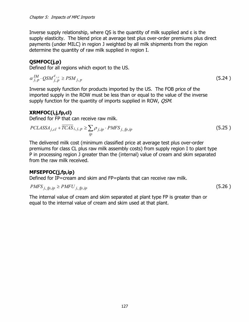
Chapter 5: Impacts of MPC Imports
127
Inverse supply relationship, where QS is the quantity of milk supplied and ε is the supply elasticity. The blend price at average test plus over-order premiums plus direct payments (under MILC) in region J weighted by all milk shipments from the region determine the quantity of raw milk supplied in region I. QSMFOC(j,p) Defined for all regions which export to the US.
pjpjIMpj PSMQSM pj
,,,, ≥⋅ εα (5.24 )
Inverse supply function for products imported by the US. The FOB price of the imported supply in the ROW must be less than or equal to the value of the inverse supply function for the quantity of imports supplied in ROW, QSM. XRMFOC(i,j,fp,cl) Defined for FP that can receive raw milk.
∑ ⋅≥+ip
ipfpjipjpjiclj PMFSTCASPCLASSA ,,,,,, ρ (5.25 )
The delivered milk cost (minimum classified price at average test plus over-order premiums for class CL plus raw milk assembly costs) from supply region I to plant type P in processing region J greater than the (internal) value of cream and skim separated from the raw milk received. MFSEPFOC(j,fp,ip) Defined for IP=cream and skim and FP=plants that can receive raw milk.
ipfpjipfpj PMFUPMFS ,,,, ≥ (5.26 )
The internal value of cream and skim separated at plant type FP is greater than or equal to the internal value of cream and skim used at that plant.
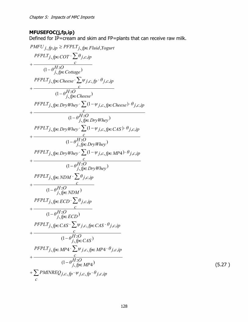
Chapter 5: Impacts of MPC Imports
128
MFUSEFOC(j,fp,ip) Defined for IP=cream and skim and FP=plants that can receive raw milk.
ipcjθfpcjψc
fpcjPMINREQ
OHMPfpjθ
cipcjθMPfpcjψMPfpjPFPLT
OHCASfpjθ
cipcjθCASfpcjψCASfpjPFPLT
OHECDfpjθc
ipcjθECDfpjPFPLT
OHNDMfpjθ
cipcjθNDMfpjPFPLT
OHDryWheyfpjθ
ipcjθc
MPfpcjψDryWheyfpjPFPLT
OHDryWheyfpjθ
ipcjθc
CASfpcjψDryWheyfpjPFPLT
OHDryWheyfpjθ
ipcjθc
CheesefpcjψDryWheyfpjPFPLT
OHCheesefpjθ
ipcjθc
fpcjψCheesefpjPFPLT
OHCottagefpjθ
cipcjθCOTfpjPFPLT
YogurtFluidfpjPFPLTipfpjPMFU
,,,,,,
)4,1(
,,4,,4,
),1(
,,,,,
),1(
,,,
),1(
,,,
),1(
,,)4,,1(,
),1(
,,),,1(,
),1(
,,),,1(,
),1(
,,,,,
),1(
,,,
,,,,
2
2
2
2
2
2
2
2
2
⋅⋅+
∈−
⋅∈⋅∈+
∈−
⋅∈⋅∈+
∈−
⋅∈+
∈−
⋅∈+
∈−
⋅∈−⋅∈+
∈−
⋅∈−⋅∈+
∈−
⋅∈−⋅∈+
∈−
⋅⋅∈+
∈−
⋅∈+
∈≥
∑
∑
∑
∑
∑
∑
∑
∑
∑
∑
(5.27 )
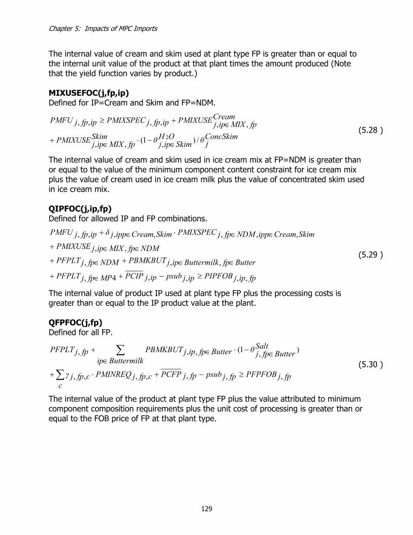
Chapter 5: Impacts of MPC Imports
129
The internal value of cream and skim used at plant type FP is greater than or equal to the internal unit value of the product at that plant times the amount produced (Note that the yield function varies by product.) MIXUSEFOC(j,fp,ip) Defined for IP=Cream and Skim and FP=NDM.
ConcSkimjθ
OHSkimipjθ
SkimfpMIXipjPMIXUSE
CreamfpMIXipjPMIXUSEipfpjPMIXSPECipfpjPMFU
/),1(,,
,,,,,,
2∈−⋅∈+
∈+≥ (5.28 )
The internal value of cream and skim used in ice cream mix at FP=NDM is greater than or equal to the value of the minimum component content constraint for ice cream mix plus the value of cream used in ice cream milk plus the value of concentrated skim used in ice cream mix. QIPFOC(j,ip,fp) Defined for allowed IP and FP combinations.
fpipjPIPFOBipjpsubipjPCIPMPfpjPFPLT
ButterfpButtermilkipjPBMKBUTNDMfpjPFPLTNDMfpMIXipjPMIXUSE
SkimCreamippNDMfpjPMIXSPECSkimCreamippjδipfpjPMFU
,,,,4,
,,,
,,
,,,,,,,
≥−+∈+
∈∈+∈+∈∈+
∈∈⋅∈+
(5.29 )
The internal value of product IP used at plant type FP plus the processing costs is greater than or equal to the IP product value at the plant. QFPFOC(j,fp) Defined for all FP.
∑
∑
≥−+⋅+
∈∈−⋅∈+
cfpjPFPFOBfpjpsubfpjPCFPcfpjPMINREQcfpjγ
Buttermilkip
SaltButterfpjθButterfpipjPBMKBUTfpjPFPLT
,,,,,,,
),1(,,, (5.30 )
The internal value of the product at plant type FP plus the value attributed to minimum component composition requirements plus the unit cost of processing is greater than or equal to the FOB price of FP at that plant type.
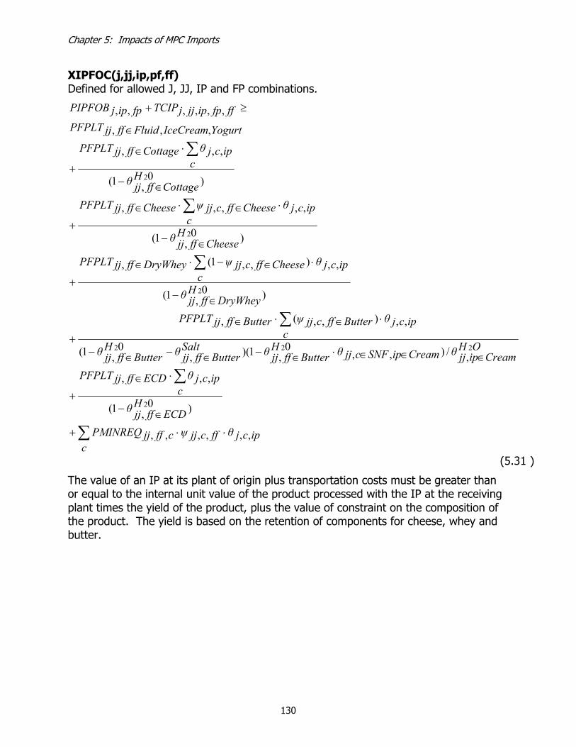
Chapter 5: Impacts of MPC Imports
130
XIPFOC(j,jj,ip,pf,ff) Defined for allowed J, JJ, IP and FP combinations.
∑
∑
∑
∑
∑
∑
⋅⋅+
∈−
⋅∈
+
∈∈∈⋅∈−∈−∈−
⋅∈⋅∈
+
∈−
⋅∈−⋅∈
+
∈−
⋅∈⋅∈
+
∈−
⋅∈
+
∈
≥+
cipcjθffcjjψcffjjPMINREQ
HECDffjjθc
ipcjθECDffjjPFPLT
OHCreamipjjθCreamipSNFcjjθ
HButterffjjθ
SaltButterffjjθ
HButterffjjθ
cipcjθButterffcjjψButterffjjPFPLT
HDryWheyffjjθ
cipcjθCheeseffcjjψDryWheyffjjPFPLT
HCheeseffjjθ
cipcjθCheeseffcjjψCheeseffjjPFPLT
HCottageffjjθ
cipcjθCottageffjjPFPLT
YogurtIceCreamFluidffjjPFPLTfffpipjjjTCIPfpipjPIPFOB
,,,,,,
)0,1(
,,,
,/),,0
,1)(,0
,1(
,,),,(,
)0,1(
,,),,1(,
)0,1(
,,,,,
)0,1(
,,,
,,,
,,,,,,
2
222
2
2
2
(5.31 )
The value of an IP at its plant of origin plus transportation costs must be greater than or equal to the internal unit value of the product processed with the IP at the receiving plant times the yield of the product, plus the value of constraint on the composition of the product. The yield is based on the retention of components for cheese, whey and butter.
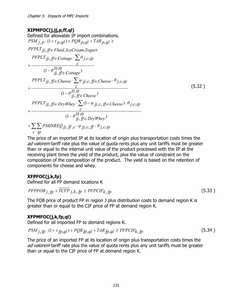
Chapter 5: Impacts of MPC Imports
131
XIPMFOC(j,jj,p,ff,ql) Defined for allowable IP import combinations.
ipcjθffcjjψc ip
cffjjPMINREQ
HDryWheyffjjθ
cipcjθCheeseffcjjψDryWheyffjjPFPLT
HCheeseffjjθ
cipcjθCheeseffcjjψCheeseffjjPFPLT
HCottageffjjθ
cipcjθCottageffjjPFPLT
YogurtIceCreamFluidffjjPFPLTqlpTARqlpPQRqlpτpjPSM
,,,,,,
)0,1(
,,),,1(,
)0,1(
,,,,,
)0,1(
,,,
,,,
,,),1(,
2
2
2
⋅⋅+
∈−
⋅∈−⋅∈
+
∈−
⋅∈⋅∈
+
∈−
⋅∈
+
∈
≥+++⋅
∑∑
∑
∑
∑
(5.32 )
The price of an imported IP at its location of origin plus transportation costs times the ad valorem tariff rate plus the value of quota rents plus any unit tariffs must be greater than or equal to the internal unit value of the product processed with the IP at the receiving plant times the yield of the product, plus the value of constraint on the composition of the composition of the product. The yield is based on the retention of components for cheese and whey. XFPFOC(j,k,fp) Defined for all FP demand locations K
fpkPFPCIFfpkjTCFPfpjPFPFOB ,,,, ≥+ (5.33 )
The FOB price of product FP in region J plus distribution costs to demand region K is greater than or equal to the CIF price of FP at demand region K. XFPMFOC(j,k,fp,ql) Defined for all imported FP to demand regions K.
fpkPFPCIFqlfpTARqlfpPQRqlfpτfpjPSM ,,,),1(, ≥+++⋅ (5.34 )
The price of an imported FP at its location of origin plus transportation costs times the ad valorem tariff rate plus the value of quota rents plus any unit tariffs must be greater than or equal to the CIF price of FP at demand region K.

Chapter 5: Impacts of MPC Imports
132
XFPXFOC(j,k,fp,xl) Defined for all subsidized FP to from supply region J=US to demand region K=ROW.
fpROWkxlfpxlfpfpUSj PFPCIFPEXSxsubPFPFOB ,,,, ∈∈ ≥+− (5.35 )
The FOB price of an US-exported FP including transportation less a unit export subsidy plus the value of a quantity constraint on subsidized exports must be greater than or equal to the CIF price of FP in the ROW. QDFOC(k,fp) Defined for all FP demand locations K.
fpk
fpkfpkfpk QDPFPCIF ,
,,,ηβ ⋅≥ (5.36 )
The CIF price of FP in region K is greater than or equal to the inverse demand relationship, where QD is the quantity demanded of product FP in region K and η is the demand elasticity for product FP in region K. MINPP(j,fp) Defined for all FP.
fpPPMINfpjPFPFOB ≥, (5.37 )
The FOB wholesale price for product P in processing region J greater than or equal to fixed minimum government purchase prices for product P.
Minimum Classified Pricing Formula Definitions
FATPR
( ), ,
,
1 11.50.82
j p j pj US p BUT
j pj US p BUT
PFPFOB QFPPRFAT
QFP∈ =
∈ =
⋅
= −
∑ ∑∑ ∑
(5.38 )
The butterfat price is equal to the weighted average FOB wholesale price of butter less a make allowance divided by a yield factor.
SNFPR
( ), ,
,
1 14.01.02
j p j pj US p NDM
j pj US p NDM
PFPFOB QFPPRSNF
QFP∈ =
∈ =
⋅
= −
∑ ∑∑ ∑
(5.39 )
The solids-not-fat (SNF) price is equal to the weighted average FOB wholesale price of nonfat dry milk (NDM) less a make allowance divided by a yield factor.

Chapter 5: Impacts of MPC Imports
133
PROTPR
( )
( )
, ,
,
, ,
,
1.405 16.5
1.28 1.582 16.5
j p j pj US p CHE
j pj US p CHE
j p j pj US p CHE
j pj US p CHE
PFPFOB QFPPRPROT
QFP
PFPFOB QFPPRFAT
QFP
∈ =
∈ =
∈ =
∈ =
⋅ = − +
⋅ − −
∑ ∑∑ ∑
∑ ∑∑ ∑
(5.40 )
The protein price is a function of the weighted average FOB wholesale price of cheddar cheese adjusted by the value of butterfat. OSPR
( ), ,
,
1 14.00.968
j p j pj US p DWH
j pj US p DWH
PFPFOB QFPPROS
QFP∈ =
∈ =
⋅
= −
∑ ∑∑ ∑
(5.41 )
The other solids (i.e. nonfat and non-protein) price is equal to the weighted average FOB wholesale price of dry whey less a make allowance and divided by a yield factor. CLFATPR(j,cl) Define for US regions J.
FMMO) (i.e., if ;,, RSTjcljcldiffPRFATcljPRFATCL =+=
( )1 and if ;1.0
,
,,
2.1, ==
−
= =
= =⋅
=∑ ∑
∑ ∑clCALj
CALj BUTppjQFP
CALj BUTppjQFPpjPFPFOB
cljPRFATCL
3/2 and if ;03815.04,, ==+== clCALjcljPRFATCLcljPRFATCL
BclCALjcljPRFATCLcljPRFATCL 4 and if ;4,, ==== (5.42 )
( )AclCALj
CALj BUTppjQFP
CALj BUTppjQFPpjPFPFOB
cljPRFATCL 4 and if ;097.0045.0,
,,
2.1, ==
−−
= =
= =⋅
=∑ ∑
∑ ∑
This equation specifies how the price of fat for each class is determined, for both FMMO and California pricing mechanisms. CLSNFPR(j,cl)
Defined for all US regions J.

Chapter 5: Impacts of MPC Imports
134
2 and if ;9/,01.0, ==⋅= clRSTjcljPRSKMCLcljPRSNFCL
1 and if ;7.8/)1,5.3464.0(76.0, ===⋅−+⋅= clCALjcljPRFATCLjCRPcljPRSNFCL
3/2 and if ;071.04,, ==+== clCALjcljPRSNFCLcljPRSNFCL (5.43 )
BclCALjcljPRFATCLjBPVCLcljPRSNFCL 4 and if ;78.8/)3,65.34(, ===⋅−=
( )AclCALj
CALj NDMppjQFP
CALj NDMppjQFPpjPFPFOB
cljPRSNFCL 4 and if ;14.0
',
',,01.0
99.0, ==−
= =
= =⋅⋅
⋅=∑ ∑
∑ ∑
This equation specifies how the price of SNF for each class is determined, for both FMMO (class II only) and California pricing mechanisms. CLSKMPR(j,cl) Defined for FMMO regions J.
( )
, 3 , 4 ,
, 4 ,
,
, ; if 1
; if 2
0.01 3.1 5.9 ;
j cl j cl j cl
j cl j cl
j RST cl
MAX PRSKMCL PRSKMCL cldiff cl
PRSKMCL cldiff cl
PRSKMCLPRPROT PROS
= =
=
=
+ =
+ =
=
⋅ ⋅ + ⋅ if 3
9 100; if 4
cl
PRSNF cl
=
⋅ =
(5.44 )
This equation specifies the price of skim milk by class for use in the FMMO pricing formulas.

Chapter 5: Impacts of MPC Imports
135
CLASSPRA(j,cl) Defined for all US regions J.
( )
( )( )
, , , ,
,, , ,
, , , ,
,, , ,
,
, ,
1; if
100
RMi c F i j p cl
i US p FPj cl
i j p cli US p FP
RMi c F i j p cl
i US p FPj cl
i j p cli US p FP
j cl
RMi c F j cl
XRMPRFATCL
XRM
XRMPRSKMCL j RST
XRM
PRCLA
PRFATCL
θ
θ
θ
=∈ ∈
∈ ∈
=∈ ∈
∈ ∈
=
⋅
+ − ⋅
=
=
⋅ +
∑ ∑∑ ∑
∑ ∑∑ ∑
( )( )( )
( )( )
, , ,
, , ,
, , , , ,
1 1 ; if , and 1
100 ; if , and 1
RM RMi c P i c S j cl
RM RM RMi c F i c P i c S j
RM RM RMi c F j cl i c P i c S j cl
PRSNFCL
PCL CAR i j CAL cl
PRFATCL PRSNFCL i j CAL cl
θ θ
θ θ θ
θ θ θ
= =
= = =
= = =
+ +
− − − = =
⋅ + + = ≠
(5.45 )
This equation determines the minimum class prices at actual test, according to both FMMO and California pricing rules. CLASSPRS(j,cl) Defined for all US regions J.
( ) ( )
( ) ( )( )
( ) ( )
, ,
, ,
,
, ,
0.035 0.965 ; if
3.5 8.7
87.8 1 ; if and 1
3.5 8.7 ;
j cl j cl
j cl j cl
j cl
j
j cl j cl
PRFATCL PRSKMCL j RST
PRFATCL PRSNFCLPRCLS
PCL CAR j CAL cl
PRFATCL PRSNFCL
+ =
+ +=
= =
+ if and 1j CAL cl
= ≠
(5.46 )
This equation determines the minimum class prices at standard test, according to both FMMO and California pricing rules. ACTCLPRA(j,cl) Defined for all US regions J.
, , ;j cl j cl jPCLASSA PRCLA OOPD j US cl CL= + ∀ ∈ ∈ (5.47 )
The actual price of milk by class, including deducts and premiums, at actual test.

Chapter 5: Impacts of MPC Imports
136
ACTCLPRS(j,cl) Defined for all US regions J.
, , ;j cl j cl jPCLASSS PRCLS OOPD j US cl CL= + ∀ ∈ ∈ (5.48 )
The actual price of milk by class, including deducts and premiums, at standard test. ACTBLEND(j) Defined for all US regions J.
j j jBLACT PBLENDA OOPD j US= + ∀ ∈ (5.49 )
The actual blend price in region j, including deducts and premiums under the PPD formula. BLENDA(j) Defined for all US regions J.
cljcl
cljj CLASSUTILPRCLAPBLENDA ,,∑ ⋅= (5.50 )
The blend price in region j at actual test, excluding deducts and premiums. BLENDS(j) Defined for all US regions J.
cljcl
cljj CLASSUTILPRCLSPBLENDS ,,∑ ⋅= (5.51 )
The blend price in region j at standard test, excluding deducts and premiums. TUTIL(j) Defined for all US regions J.
∑∑∑∑∑∑ +=jj ip ff fp
fpffipjjjip fp
ipfpjj XIPQMFUSETOTUTIL ,,,,,, (5.52 )
CU(j) Defined for all US regions J.
j
jj ip ff fpfpffipjjj
ip fpipfpj
clj TOTUTIL
XIPQMFUSE
CLASSUTIL∑∑∑∑∑∑ +
=,,,,,,
, (5.53 )
DIRECT(j) Defined for all US regions J.
( )( ){ }, 10, 0.45 16.94 3.25 2.69
j
j j RST cl j RST
DP
PEM MAX PCLASSS OOPD j US′ ′= = =
=
⋅ − − − − ∀ ∈ (5.54 )
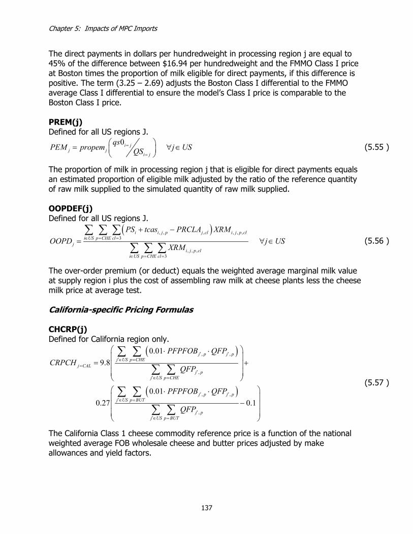
Chapter 5: Impacts of MPC Imports
137
The direct payments in dollars per hundredweight in processing region j are equal to 45% of the difference between $16.94 per hundredweight and the FMMO Class I price at Boston times the proportion of milk eligible for direct payments, if this difference is positive. The term (3.25 – 2.69) adjusts the Boston Class I differential to the FMMO average Class I differential to ensure the model’s Class I price is comparable to the Boston Class I price. PREM(j) Defined for all US regions J.
0 i jj j
i j
qsPEM propem j USQS=
=
= ∀ ∈
(5.55 )
The proportion of milk in processing region j that is eligible for direct payments equals an estimated proportion of eligible milk adjusted by the ratio of the reference quantity of raw milk supplied to the simulated quantity of raw milk supplied. OOPDEF(j) Defined for all US regions J.
( ), , , , , ,3
, , ,3
i i j p j cl i j p cl
i US p CHE clj
i j p cli US p CHE cl
PS tcas PRCLA XRMOOPD j US
XRM∈ = =
∈ = =
+ −= ∀ ∈∑ ∑ ∑
∑ ∑ ∑ (5.56 )
The over-order premium (or deduct) equals the weighted average marginal milk value at supply region i plus the cost of assembling raw milk at cheese plants less the cheese milk price at average test. California-specific Pricing Formulas CHCRP(j) Defined for California region only.
( )
( )
, ,
,
, ,
,
0.019.8
0.010.27 0.1
j p j pj US p CHE
j CALj p
j US p CHE
j p j pj US p BUT
j pj US p BUT
PFPFOB QFPCRPCH
QFP
PFPFOB QFP
QFP
′ ′′∈ =
=′
′∈ =
′ ′′∈ =
′′∈ =
⋅ ⋅
= + ⋅ ⋅
−
∑ ∑∑ ∑
∑ ∑∑ ∑
(5.57 )
The California Class 1 cheese commodity reference price is a function of the national weighted average FOB wholesale cheese and butter prices adjusted by make allowances and yield factors.
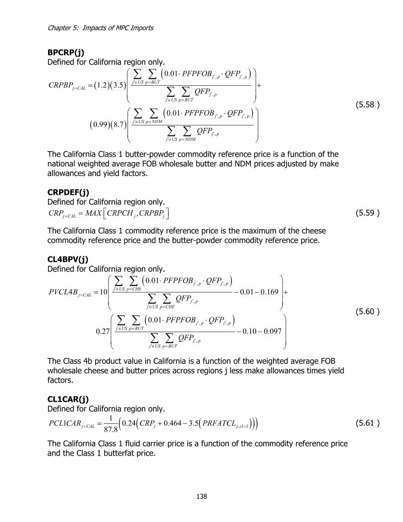
Chapter 5: Impacts of MPC Imports
138
BPCRP(j) Defined for California region only.
( )( )( )
( )( )( )
, ,
,
, ,
,
0.011.2 3.5
0.010.99 8.7
j p j pj US p BUT
j CALj p
j US p BUT
j p j pj US p NDM
j pj US p NDM
PFPFOB QFPCRPBP
QFP
PFPFOB QFP
QFP
′ ′′∈ =
=′
′∈ =
′ ′′∈ =
′′∈ =
⋅ ⋅
= + ⋅ ⋅
∑ ∑∑ ∑
∑ ∑∑ ∑
(5.58 )
The California Class 1 butter-powder commodity reference price is a function of the national weighted average FOB wholesale butter and NDM prices adjusted by make allowances and yield factors. CRPDEF(j) Defined for California region only.
,j CAL j jCRP MAX CRPCH CRPBP= = (5.59 )
The California Class 1 commodity reference price is the maximum of the cheese commodity reference price and the butter-powder commodity reference price. CL4BPV(j) Defined for California region only.
( )
( )
, ,
,
, ,
,
0.014 10 0.01 0.169
0.010.27 0.10 0.097
j p j pj US p CHE
j CALj p
j US p CHE
j p j pj US p BUT
j pj US p BUT
PFPFOB QFPPVCL B
QFP
PFPFOB QFP
QFP
′ ′′∈ =
=′
′∈ =
′ ′′∈ =
′′∈ =
⋅ ⋅
= − − + ⋅ ⋅
− −
∑ ∑∑ ∑
∑ ∑∑ ∑
(5.60 )
The Class 4b product value in California is a function of the weighted average FOB wholesale cheese and butter prices across regions j less make allowances times yield factors. CL1CAR(j) Defined for California region only.
( )( )( ), 111 0.24 0.464 3.5
87.8j CAL j j clPCL CAR CRP PRFATCL= == + − (5.61 )
The California Class 1 fluid carrier price is a function of the commodity reference price and the Class 1 butterfat price.

Chapter 5: Impacts of MPC Imports
139
Variables and Parameters
The variables and parameters used in the above equations are: QSi = Quantity of milk supplied in supply region I
XRMi,j,fp,cl = Quantity of raw milk shipped from supply region I to plant type P (in class CL) in processing region J
ρj,ip = Proportion of IP=cream and skim separated from milk received at plants in region J.
QMFSEPj,fp,ip = Volume of IP=cream and skim separated from raw milk received at plant type FP in region J.
QMFUSEj,fp,ip = Volume of IP=cream and skim used in FP at plant type FP in region J.
QUSEMIXj,fp,ip = Volume of IP=cream and skim used in IP=ice cream mix at FP=NDM in region J.
QIP j,ip,p = Quantity of intermediate product IP processed at plant type P in region J.
J.regionat IPproduct teintermedia inwater of Proportion , =OHipjθ2
Jregionat skim edconcentrat in solids total of Proportion =ConcSkimjθ
mix cream ice in used skim and cream of Proportion =∈ SkimCreamipj ,,δ
XIPj,jj,ip,p,pp = Quantity of intermediate product IP shipped from plant type P in region J to plant type PP in region JJ
XIPMjj,j,ip,fp,ql = Quantity of imported intermediate product IP shipped from region JJεROW to plant type FP in region J under quota level QL
QFPj,p = Quantity of final product P processed at plant type P in region J
Jregion in processed IPproduct teintermedia in Ccomponent of Proportion ,, =ipcjθ
Jregion in processed FPproduct final inwater of Proportion , =OHfpjθ2
Jregion in processed FPproduct final in Ccomponent of Retention ,, =fpcjψ
FPproduct final insalt of Proportion =Saltfpθ
Jregion in processed FPproduct final in Ccomponent of proportion Minimum =cfpj ,,γ

Chapter 5: Impacts of MPC Imports
140
XFPj,k,fp = Quantity of final product FP shipped from region J to demand region K
XFPGj,p = Quantity of final product FP shipped from region J to government purchase programs
QSMjεROW,p = Quantity of imports of final product P supplied by region J=ROW
XFPMjεROW,k,p,ql = Quantity of imports of final product P shipped from region J=ROW to US demand region K under quota level QL
xvolfp,xl = Limit of exports for final product FP under export subsidy level XL
XFPXj,kεROW,fp,xl = Quantity of final product FP exports shipped from US region J to demand region K=ROW under export subsidy level XL
QDk,p = Quantity of final product P demanded in demand region K
qlvl p,ql = Limit of imports for intermediate and final product P under import quota level QL
αi = Inverse raw milk supply parameter in supply region I
εi = Raw milk supply flexibility in supply region I
BLACTj = Blend price plus over-order premiums in region J (All-milk price in region J) at actual test
DPj = Direct payments under MILC per hundredweight of milk in region J
parametersupply product imported Inverse , =IMpjα
PSMj,p = Price of imported intermediate or final product.
PCLASSAj,cl = Class price of milk at actual test plus over-order premiums (actual milk cost to processors)
Jregion processing in
P typeplant to I regionsupply fromassembly milk raw ofCost =pjiTCAS ,,
PMFSj,fp,ip = Marginal value of IP=cream and skim at separation at plant type FP in region J
PMFUj,fp,ip = Marginal value of IP=cream and skim at use in final products at plant type FP in region J
PFPLTj,fp = Marginal (internal) value a unit of final product at plant type FP in region J
PMINREQj,c,fp = Marginal value of minimum required composition of component C in product FP in region J

Chapter 5: Impacts of MPC Imports
141
PMIXSPECj, fp, ip = Marginal value of minimum required composition of ice cream mix in region J
PMIXUSEj,ipεMIX,fp = Marginal value of cream and skim used in ice cream mix in region J
PBMKBUTj, ipεButtermilk, fpεButter = Value of buttermilk at butter plant in region J
Jregion processing in IPproduct ofcost processingUnit =,fpjPCIP
PIPFOBj,ip,fp = FOB wholesale price for intermediate product IP produced at plant type FP in processing region J
PFPFOBj,fp = FOB wholesale price for final product FP in processing region J
Jregion processing in FPproduct ofcost processingUnit , =fpjPCFP
PFPFOBj,p = FOB wholesale price for product P in processing region J
pppipjjjTCIP ,,,, = Cost of transporting intermediate product IP from plant type P in
processing region J to plant type PP in processing region JJ
QL level quotaunder Pproduct of imports on tariff valorem Ad, =qlpτ
QL level quotaunder Pproduct of imports on nrestrictio quota of valueMarginal , =qlpPQR
QL level quotaunder Pproduct of imports on tariffUnit =qlpTAR ,
K region demand to J
region processing from FPproduct final of ondistributi wholesale ofCost =fpkjTCFP ,,
PFPCIFkf,p = CIF wholesale price for final product FP in demand region K
xsubfp,xl = Unit export subsidy for final product FP under export subsidy level XL
PEXSfp,xl = Marginal value of constraint of quantity of FP exported under export subsidy level XL
βk,fp = Inverse wholesale demand parameter for final product FP in demand region K
ηk,fp = Final product FP demand flexibility in region K
Pproduct for price purchase government minimum Fixed =pPPMIN
PRFAT = Butterfat price from FMMO pricing formulas
PRSNF = SNF price from FMMO pricing formulas

Chapter 5: Impacts of MPC Imports
142
PROS = Other solids price from FMMO pricing formulas
PRPROT = Protein price from FMMO pricing formulas
PRFATCLj, cl = Price of butterfat for class CL in region J
PRSNFCLj, cl = Price of SNF for class CL in region J
PRSKMCLjεRST, cl = Price of skim for class CL in region J
PRCLAj, cl = Minimum class price for class CL in region J at actual test
PRCLSj, cl = Minimum class price for class CL in region J at standard test
PCLASSAj, cl = Actual cost of milk used class CL in region J at actual test, including premiums or deducts
PCLASSSj, cl = Actual cost of milk used class CL in region J at standard test, including premiums or deducts
OOPDj = Over-order premium in processing region J
PBLENDAj = Blend price of milk used in region J at actual test
PBLENDSj = Blend price of milk used in region J at standard test
TOTUTILj = Total utilization of cream and skim and interplant shipments in region J
CLASSUTILj,cl = Total utilization of cream and skim and interplant shipments in class CL in region J
PEMj = Proportion of milk in processing region J eligible for direct payments
paymentsdirect for eligible Jregion processing in milk of proportion Initial =jPROPEM PSi = Marginal value of raw milk at supply point I
CRPCHjεCAL= Commodity reference price for cheese from California pricing formulas
CRPBPjεCAL = Commodity reference price for butter-powder from California pricing formulas
CRPjεCAL = Commodity reference price for Class 1 from California pricing formulas
PVCL4bjεCAL = Class 4b product value price from California pricing formulas
PCL1CARjεCAL = Class 1 fluid carrier price from California pricing formulas


![RBEs and MPCs in MSC.nastran2[1]](https://static.fdocuments.us/doc/165x107/577d20d31a28ab4e1e93d88c/rbes-and-mpcs-in-mscnastran21.jpg)


