University of Huddersfield Repository

Ward, C.P., Dixon, R. and Goodall, Roger M.

Wheel­Rail Profile Condition Monitoring

Original Citation

Ward, C.P., Dixon, R. and Goodall, Roger M. (2010) Wheel­Rail Profile Condition Monitoring. In: UKACC International Conference on Control 2010, 7th ­ 10th September 2010, Coventry, UK.

This version is available at http://eprints.hud.ac.uk/id/eprint/17879/

The University Repository is a digital collection of the research output of theUniversity, available on Open Access. Copyright and Moral Rights for the itemson this site are retained by the individual author and/or other copyright owners.Users may access full items free of charge; copies of full text items generallycan be reproduced, displayed or performed and given to third parties in anyformat or medium for personal research or study, educational or not­for­profitpurposes without prior permission or charge, provided:

• The authors, title and full bibliographic details is credited in any copy;• A hyperlink and/or URL is included for the original metadata page; and• The content is not changed in any way.

For more information, including our policy and submission procedure, pleasecontact the Repository Team at: E.mailbox@hud.ac.uk.

http://eprints.hud.ac.uk/

Wheel-Rail Profile Condition Monitoring

Christopher P. Ward ∗ Roger M. Goodall ∗ Roger Dixon ∗

∗ Department of Electronic and Electrical Engineering, LoughboroughUniversity, Loughborough, Leicestershire, LE11 3TU, UK(e-mail:

c.p.ward@lboro.ac.uk; r.m.goodall@lboro.ac.uk; r.dixon@lboro.ac.uk)

Abstract: Increased railway patronage worldwide is putting pressure on rolling stock and in-frastructure to operate at higher capacity and with improved punctuality. Condition monitoringis seen as a contributing factor in enabling this and is highlighted here in the context of rollingstock being procured with high capacity data buses, multiple sensors and centralised control.This therefore leaves scope for advanced computational diagnostic concepts. The rail vehiclebogie and associated wheelsets are one of the largest and most costly areas of maintenance onrolling stock and presented here is a potential method for real time estimation of wheel-railcontact wear to move this currently scheduled based assessment to condition based assessment.This technique utilises recursive ‘grey box’ least squares system identification, used in a piecewiselinear manner, to capture the strongly discontinuous nonlinear nature of the wheel-rail geometry.

Keywords: Accelerometers, Fault Diagnosis/Detection, Kalman Filters, Nonlinear Systems,Piecewise Linear Analysis, Recursive Least Squares, Railways, Vehicle Dynamics

1. INTRODUCTION

Increased patronage of railways worldwide in the past twodecades has put pressure on rolling stock and engineeringinfrastructure to operate at a higher capacity and withincreased punctuality. This therefore creates a demand onmaintenance systems to reduce the time rolling stock is outof service due to condition checks and regular servicing.Contemporary trains are being built with high capacitycommunication buses and numerous sensors at importantlocations on the vehicle. This means there is scope for theapplication of advanced numerical methods for conditionmonitoring of key components in real time.

One such component is the railway vehicle bogie and itsassociated wheelsets, consisting of two wheels solidly fixedto an axle. This system is responsible for one of the largestareas of maintenance costs of the entire system and istherefore one of the key targets for condition monitoring.This paper covers; context of wheel-rail profile estima-tion; development of simulation models that include gaugewidth variation with the use of disturbance signals morerepresentative of the frequency content of real track geom-etry; and development of a recursive identification processusing a linear piecewise approach to identify rolling radiiand contact angles of the wheel-rail interaction instead ofthe effective conicity. This last point was previously brieflydescribed in Ward et al. (2010) and is expanded here.Further discussion is made of: a potential looped trackdisturbance estimation with geometry estimation concept;signal frequency content analysis of different wear statesof wheelsets along a section of track; and the potential useof creep force estimation to determine the condition of thewheel-rail interface, Charles et al. (2008c).

This work carries on research performed in various sourcesto determine the wheel-rail profile. Initially Li et al. (2003),Li et al. (2004) and Li et al. (2006) showed that con-

dition monitoring of suspension components such as sec-ondary dampers can be achieved in real time using Rao-Blackwellised Particle Filters (RBPF). This was less suc-cessful at monitoring the condition of wear of the wheelsetin combination with the rail, known as a linearised effectiveconicity function, λ. Further investigations of linear conic-ity estimation were covered in Selamat and Yusof (2009),with the limitation that the model was linear and that thelateral rail irregularity was known.

Ideas for the estimation of a nonlinear conicity were ex-plored initially in Charles et al. (2008c) using ExtendedKalman-Bucy Filtering (EKBF). Later Charles et al.(2008b) and Charles et al. (2008a) used a Piecewise CubicPolynomial (PCP) function in a least squares identificationof the nonlinear conicity. The Kalman filter technique hadweaknesses at larger relative displacements of the wheelsetto the rail and the system identification method requireda knowledge of the exact input to the system, the lateraltrack disturbance d. This last point may be unfeasible inapplication or may require estimation.

2. WHEELSETS AND CURRENT PRACTICE

Railway vehicles’ wheelsets and how they interact withthe railhead are the most fundamental component of arailway vehicle. Two coned and flanged wheels connectedsolidly to a central shaft provide: straight line guidanceto negate the effect of stochastic lateral rail irregularities;cornering performance; braking traction; accelerative trac-tion; and ride characteristics, Iwnicki (2006). Therefore,the condition of these components is of safety criticalimportance for the operation of the whole system. If thegeometry of the wheelset in combination with that of therailhead moves out of allowable tolerance, the rail vehiclecan become dynamically unstable and potentially causevehicle derailment, Wickens (2003). This relationship is

highly nonlinear as the wheel treads are not perfectlyconed and the railheads are not point contact, but domed,an example of which is shown in Figure 1.

Fig. 1. Wheel profile and railhead cross section

At present, the level of wear in the wheel tread andthe railhead are monitored separately with the use ofphysical measuring devices, such as the MiniProf system,Greenwood-Engineering (2010). This is time consuming,costly and could potentially miss a wheelset or railheadin dangerous condition in-between inspection intervals.Therefore, a system that can detect the level of wearin the wheel-rail contact geometry in real-time is highlydesirable. This would make use of cost effective and reliableinertial sensors positioned around the bogie system, withprocessing performed by advanced filtering.

Condition monitoring is currently becoming more preva-lent in rail vehicles. They are being manufactured withmultiple sensors, high capacity communication buses andpowerful processing capability. One such system in oper-ation is Bombardier Transportation Orbita, Bombardier(2010), which followed trends set in the aerospace andautomotive industries where knowledge of fleet conditioncan be built up through health monitoring systems. Theideas proposed here could be integrated into such a system.

3. WHEELSET AND VEHICLE MODELS

The research presented is in the proof of concept stage andso was initially developed using a simple model for simula-tion, consisting of a single wheelset and single suspendedmass (Figure 2). As the work progresses more complexmodels will be used. Due to minimal coupling betweenlateral, longitudinal and vertical planes, the wheelset dy-namics are considered with only lateral displacement, yawrotation and roll rotation, with the suspended mass con-taining only lateral displacement dynamics. A simplifiednonlinear model is taken from Garg and Dukkipati (1984),where the equation for the lateral dynamics of the wheelsetis

Fig. 2. Wheelset and mass model

my +2f22V

(y +

(rL + rR)

2φ− V ψ

)

+2f11

(1−

(rL + rR)

2r0

)ψ

+ 2f23

(ψ

V−

(δL − δR)

2r0

)

+W

((δL − δR)

2+ φ

)= Fsy

(1)

which consists of the longitudinal creep force, lateral creepforce, lateral/spin creep force and gravitational creep force.The yaw dynamics equation for the wheelset is

Iψ + IwyV

r0φ+

2l2f11r0

((rL − rR)

2l

)

−2f23V

(y +

(rL + rR)

2φ− V ψ

)

+ 2l2f11ψ

V− 2f33

(δL − δR)

2r0

−lW(δL + δR)

2ψ + 2f33

ψ

V= Msψ

(2)

which consists of the roll moment, longitudinal creepmoment, lateral/spin creep moment, spin creep momentand the gravitational stiffness moment. The equation forthe lateral dynamics of the suspended mass is

y =1

mm

(Fsy) (3)

the lateral suspension forces is

Fsy = ky(ym − y) + fy(ym − y) (4)

and the suspension yaw force is

Msψ = −kψψ − fψψ (5)

Parameters and states for all of the equations are given inTable A.1.

The significant nonlinearities in the equations are in theform of static geometric relationships of the rolling radiiand contact angles, rL rR δL δR. These are calculatedfor specific wheel-rail combinations by a Newton-Raphsoniterative process, Wickens (2003), and are function of therelative displacement of the wheelset to the railhead, (y−d). Example profiles for a P8 wheel profile and a 113A

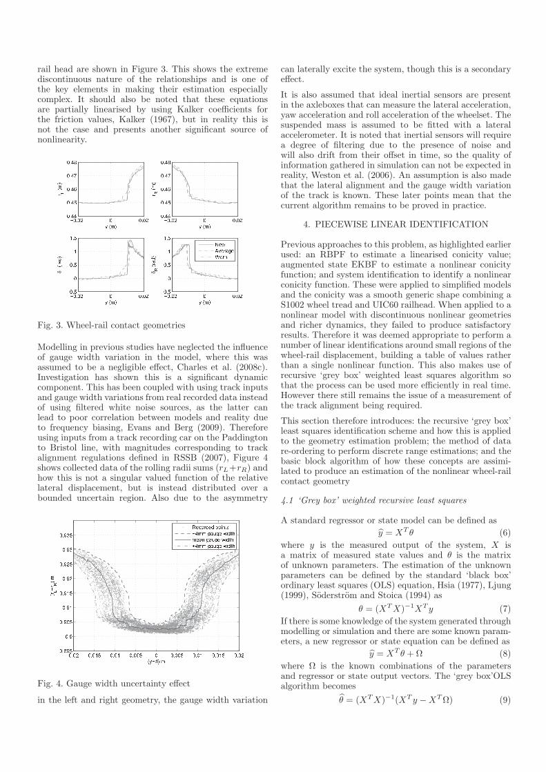
rail head are shown in Figure 3. This shows the extremediscontinuous nature of the relationships and is one ofthe key elements in making their estimation especiallycomplex. It should also be noted that these equationsare partially linearised by using Kalker coefficients forthe friction values, Kalker (1967), but in reality this isnot the case and presents another significant source ofnonlinearity.

!

"

δ

! #$ δ

" #$ % & ' ( )Fig. 3. Wheel-rail contact geometries

Modelling in previous studies have neglected the influenceof gauge width variation in the model, where this wasassumed to be a negligible effect, Charles et al. (2008c).Investigation has shown this is a significant dynamiccomponent. This has been coupled with using track inputsand gauge width variations from real recorded data insteadof using filtered white noise sources, as the latter canlead to poor correlation between models and reality dueto frequency biasing, Evans and Berg (2009). Thereforeusing inputs from a track recording car on the Paddingtonto Bristol line, with magnitudes corresponding to trackalignment regulations defined in RSSB (2007), Figure 4shows collected data of the rolling radii sums (rL+rR) andhow this is not a singular valued function of the relativelateral displacement, but is instead distributed over abounded uncertain region. Also due to the asymmetry

* * * * * * * * *

!+ " , - ) . / ' 0 ' . ) ' 0 ' . 1 ' 0 ' . Fig. 4. Gauge width uncertainty effect

in the left and right geometry, the gauge width variation

can laterally excite the system, though this is a secondaryeffect.

It is also assumed that ideal inertial sensors are presentin the axleboxes that can measure the lateral acceleration,yaw acceleration and roll acceleration of the wheelset. Thesuspended mass is assumed to be fitted with a lateralaccelerometer. It is noted that inertial sensors will requirea degree of filtering due to the presence of noise andwill also drift from their offset in time, so the quality ofinformation gathered in simulation can not be expected inreality, Weston et al. (2006). An assumption is also madethat the lateral alignment and the gauge width variationof the track is known. These later points mean that thecurrent algorithm remains to be proved in practice.

4. PIECEWISE LINEAR IDENTIFICATION

Previous approaches to this problem, as highlighted earlierused: an RBPF to estimate a linearised conicity value;augmented state EKBF to estimate a nonlinear conicityfunction; and system identification to identify a nonlinearconicity function. These were applied to simplified modelsand the conicity was a smooth generic shape combining aS1002 wheel tread and UIC60 railhead. When applied to anonlinear model with discontinuous nonlinear geometriesand richer dynamics, they failed to produce satisfactoryresults. Therefore it was deemed appropriate to perform anumber of linear identifications around small regions of thewheel-rail displacement, building a table of values ratherthan a single nonlinear function. This also makes use ofrecursive ‘grey box’ weighted least squares algorithm sothat the process can be used more efficiently in real time.However there still remains the issue of a measurement ofthe track alignment being required.

This section therefore introduces: the recursive ‘grey box’least squares identification scheme and how this is appliedto the geometry estimation problem; the method of datare-ordering to perform discrete range estimations; and thebasic block algorithm of how these concepts are assimi-lated to produce an estimation of the nonlinear wheel-railcontact geometry

4.1 ‘Grey box’ weighted recursive least squares

A standard regressor or state model can be defined as

y = XT θ (6)

where y is the measured output of the system, X isa matrix of measured state values and θ is the matrixof unknown parameters. The estimation of the unknownparameters can be defined by the standard ‘black box’ordinary least squares (OLS) equation, Hsia (1977), Ljung(1999), Soderstrom and Stoica (1994) as

θ = (XTX)−1XT y (7)

If there is some knowledge of the system generated throughmodelling or simulation and there are some known param-eters, a new regressor or state equation can be defined as

y = XT θ + Ω (8)

where Ω is the known combinations of the parametersand regressor or state output vectors. The ‘grey box’OLSalgorithm becomes

θ = (XTX)−1(XT y −XTΩ) (9)

This format is a ‘block’ identification, where all of the datacollected is used to determine the unknown parameters. Inthis application data from the system will be collected inreal time and as such an updating process is needed thatwill adapt with time as new data is collected. The ‘blackbox’ and ‘grey box’ OLS algorithms can be applied in suchas manner, Astrom (1989). A weighting factor can also beadded to ‘forget’ previous measurements, thus being moreor less receptive to new data. Initial conditions for the‘grey box’ recursive least squares version of the algorithmare set as

P(0) =(XT

(0)X(0)

)−1

(10)

θ(0) = P(0)

(XT

(0)y(0) −XT(0)Ω(0)

)(11)

where X(0) is the matrix of state values up to the startof the identification process, y(0) is the initial outputvector and θ(0) is the initial least squares estimation. Theestimation loop is then performed recursively as data isadded to the X matrix as

γ(i) =1

W +XT(i)P(i−1)X(i)

(12)

P(i) =(P(i−1) − γ(i)P(i−1)X

T(i)X(i)P(i−1)

) 1

W(13)

θ(i) =θ(i−1) +(γ(i)P(i−1)X

T(i)

((y(i) − Ω(i)

)

−(X(i)θ(i−1)

))) (14)

where 0 < W ≤ 1 is the updating weighting factor andi is the number of the iteration. This format also savescomputational expense as only the latest added values areacted upon rather than the entire data set.

In this application each estimation is performed using twomultiple-input-single-output identifications. The first is are-arrangement of the lateral wheelset dynamics (Equation1) to make the lateral acceleration y the subject, from thisthe known parameter equation becomes

Ω1 =

(−

2f22mv

−fy

m

)y +

(−ky

m

)y +

(fy

m

)ym

+

(ky

m

)ym +

(−

2f23mv

)ψ +

(−W

m

)φ

(15)

and the X matrix becomes

X1 =[ψ, φ, 1

](16)

The second estimation uses the wheelset yaw dynamics(Equation 2) in the form of the yaw acceleration ψ, fromwhich the known parameter equation becomes

Ω2 =

(−

2f23Iv

)y +

(−

2l2f11Iv

−2f33Iv

−fψ

I

)ψ (17)

and the corresponding X matrix is

X2 =[ψ, φ, 1

](18)

Estimates of the corresponding parameters can then bemanipulated to determine the parameter combinations(rL + rR), (rL − rR), (δL + δR) and (δL − δR).

4.2 Data splitting

The recursive least squares estimation of the previoussection is applied to discrete sections of data relative to thewheel-rail displacement. Therefore this data first requires

ordering from the main data stream. This separation isperformed relative to the displacement (y−d), therefore ifthe data is of the length n, the range of the data is definedas

a = max(y − d)−min(y − d) (19)

where b is the user defined division size, the number ofsections that the data is separated becomes

n =a

b(20)

The data is then partitioned into one of the n bins. If thenumber of bins is defined as j = 1 : n and the time intervalis defined as i, the current collected piece of data (y − d)iis checked to see if

aj > (y − d)i > a(j − 1) (21)

If this statement is true the data is stored in bin j.Correspondingly the data for all the other states at timei are stored in bins numbered j. This process occursrecursively so that as new data is collected it is checkedfor relative position and stored in the corresponding bin.

This separation of data works here due to the very stiffnature of the system. Meaning that there is very littletime delay present and therefore the states of the systemmatch up as the data transitions in and out of the divisionsections, though inevitably some correlation will be lost.

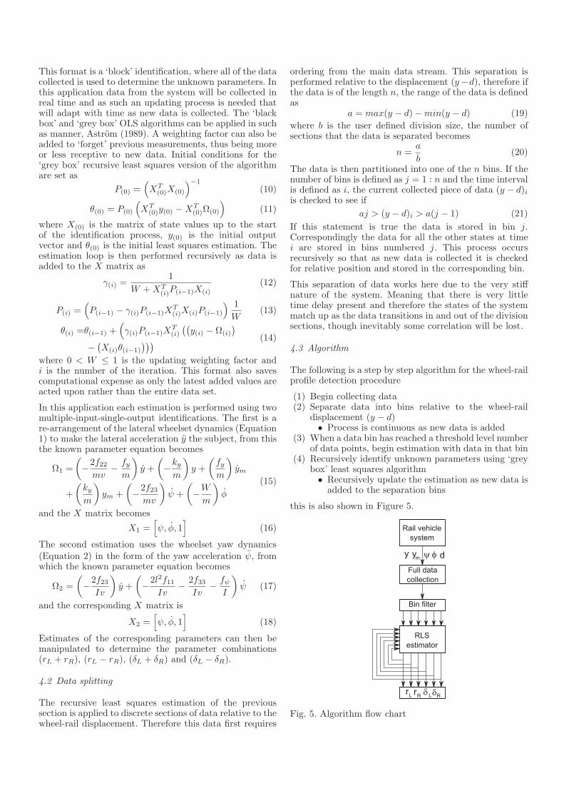
4.3 Algorithm

The following is a step by step algorithm for the wheel-railprofile detection procedure

(1) Begin collecting data(2) Separate data into bins relative to the wheel-rail

displacement (y − d)• Process is continuous as new data is added

(3) When a data bin has reached a threshold level numberof data points, begin estimation with data in that bin

(4) Recursively identify unknown parameters using ‘greybox’ least squares algorithm• Recursively update the estimation as new data is

added to the separation bins

this is also shown in Figure 5.

Fig. 5. Algorithm flow chart

5. EXAMPLE APPLICATION

The above algorithm was applied to the single wheelsetsystem and suspended mass in two configurations, the firstwith no gauge width variation as the second with gaugewidth variation. Values of the parameters used for thesimulation are also shown in Table A.1 where applicable.

Simulations were run with P8 shaped wheelsets in amedium state of wear having covered 117,000 miles on aclass 43 power car and a 113A railhead in a new state. Thesystem was excited by lateral misalignment of the railheadwith a standard deviation (STD) of approximately 2mm,and with a gauge width variation also with an STD ofapproximately 2mm. Both misalignments were recored onthe Paddington to Bristol line using a track recording car.

The estimation was first performed with no gauge widthvariation present. As expected this produces a good esti-mation of the model parameters, this is shown in Figure 6for the rolling radii sums, (rL + rR). Though not shown,the remaining three geometric combinations also give goodcorrelation.

* * * * * * !+ "

2 2 )2 1 3 / . . )Fig. 6. Estimation with no gauge width variation

The second estimation is performed with gauge widthvariation in the simulation. This does not produce as goodan estimation due to there now being uncertainty in theparameters. Figure 7 shows the estimation again for therolling radii sums. The estimation points now occupy anestimation space within the boundaries set by the gaugewidth variation. Although not shown the contact anglesum fails to converge completely. This may be due tothe parameter being highly dependent upon knowing thegauge width exactly.

6. FUTURE WORK AND POSSIBLE APPROACHES

The main issue with the algorithm highlighted in thispaper is the need to know the input irregularity andthe gauge width variation. This would be difficult andexpensive to practically measure in real time for eachwheelset using a vision or laser based system. It is possiblethat track recording data might be exploited but precisesynchronisation means that this is not straight forward.Another possible solution is to estimate the disturbance

* * * * * * !+ "

2 2 )2 1 3 / . . )Fig. 7. Estimation with gauge width variation

signal with an assumed geometric formation, then feedthis estimate into the identification. This would becomea looped process with the disturbance estimation runningat a faster rate than the geometric estimation, a schematicof which is shown in Figure 8. However this estimation will

Fig. 8. Looped estimator

also be a highly complex nonlinear algorithm.

To negate the need to have the exact disturbance signal,solutions could rely on a statistical analysis. Initial workhas begun to look at the frequency content of raw mea-sured signals for various conditions of wheelsets along thesame section of track. This has shown some difference andcould therefore be used to build a library that could bereferenced against signals collected in operation, thereforegiving an indication of the wear state. However this wouldrequire a great deal more user input. Similar possibilitiesare to analyse the force estimation that is proposed for lowadhesion estimation, Charles et al. (2008c).

7. CONCLUSION

This paper discussed a potential algorithm for the realtime estimation of the wheel-rail contact geometry in railvehicle systems. This interaction is important due to itgoverning the straight line running stability and corneringperformance of rail vehicles. The recursive least squaresalgorithm proposed uses a series of piecewise linear es-timations due to the strongly discontinuous nature of thecontact geometry, where the dynamic data is sectioned rel-ative to the wheel-rail displacement. With no gauge widthvariation this gives excellent correlation with the inputtedgeometry, but begins to decorrelate when uncertainty inthe gauge width is added to the system. The techniquealso relies upon a knowledge of the track disturbanceto perform the estimation that might not be practicablyfeasible.

Further proposals were made to negate the problemsof track alignment measurement, such as; estimation ofthe track disturbance using a known geometry; usingstatistical analysis of measured signals from the wheelsetthat correspond to specific wear states along a section oftrack; or using statistical information from the estimationof creep forces in the contact area.

ACKNOWLEDGEMENTS

The authors would like to thank Rail Research UnitedKingdom (RRUK) and the Engineering and Physical Sci-ence Research Council (EPSRC) who funded this research.Additional thanks to the Rail Technology Unit (RTU)at Manchester Metropolitan University (MMU) who pro-vided track and vehicle data for the study.

REFERENCES

Astrom, K. (1989). Adaptive control. Addison-Wesley, firstedition.

Bombardier (2010). Orbita - predictive assetmanagement, the future of fleet maintenance.http://www.bombardier.com/en/transportation/accessed 7th April 2010.

Charles, G., Dixon, R., and Goodall, R. (2008a). Condi-tion Monitoring Approaches to Estimating Wheel-RailProfile. In Proceedings of UKACC Control Conference,Manchester.

Charles, G., Goodall, R., and Dixon, R. (2008b). ALeast Mean Squared Approach to Wheel-Rail ProfileEstimation. In Proceedings of the 4th InternationalConference On Railway Condition Monitoring.

Charles, G., Goodall, R., and Dixon, R. (2008c). Model-based condition monitoring at the wheel-rail interface.Vehicle System Dynamics, 46(1), 415–430.

Evans, J. and Berg, M. (2009). Challenges in simulation ofrail vehicle dynamics. International Journal of VehicleMechanics and Mobility, (8), 1023–1048.

Garg, V. and Dukkipati, R. (1984). Dynamics of RailwayVehicle Systems. Academic Press, first edition.

Greenwood-Engineering (2010). MiniProf - the profileof measuring. http://www.greenwood.dk/miniprof.phpaccessed 7th April 2010.

Hsia, T. (1977). System Identification, Least-SquaresMethods. Lexington Books, first edition.

Iwnicki, S. (2006). Handbook of Railway Vehicle Dynamics.Taylor and Francis, first edition.

Kalker, J. (1967). On the Rolling Contact of Two ElasticBodies in the Presence of Dry Friction. Ph.D. thesis,Delft University of Technology, Delft, Netherlands.

Li, P., Goodall, R., and Kadirkamanathan, C. (2003).Parameter estimation of railway vehicle dynamic modelusing rao-blackwellised particle filter. In Proceedingsof the seventh European control conference, Cambridge,UK.

Li, P., Goodall, R., and Kadirkamanathan, C. (2004). Es-timation of parameters in a linear state space model us-ing a rao-blackwellised particle filter. IEE Proceedings-Control Theory and Applications, 151:727-738.

Li, P., Goodall, R., Weston, P., Ling, C., Goodman,C., and Roberts, C. (2006). Estimation of railwayvehicle suspension parameters for condition monitoring.Control Engineering Practice, 15:43-55.

Ljung, A. (1999). System Identification, Theory for theUser. Prentice Hall, second edition.

RSSB (2007). Track System Requirements GC/RT5021.Rail Safety and Standards Board Limited, third edition.

Selamat, H. and Yusof, R. (2009). Wheel-rail contactparameters estimation for a conical solid-axle railwaywheelset using least-absolute error with variable forget-ting factor method. In Proceedings of the 2009 IEEEInternational Conference on Industrial Technology.

Soderstrom, T. and Stoica, P. (1994). System Identifica-tion. Prentice Hall, second edition.

Ward, C., Weston, P., Stewart, E., Li, H., Goodall, R.,Roberts, C., Mei, T., Charles, G., and Dixon, R. (2010).Condition monitoring opportunities using vehicle basedsensors. Awaiting publication: IMechE proceedings, PartF: Rail and Rapid Transit.

Weston, P., Ling, C., Goodman, C., Roberts, C., Li, P., andGoodall, R. (2006). Monitoring lateral track irregularityfrom in-service railway vehicles. IMechE proceedings,Part F: Rail and Rapid Transit, 221(RRUK SpecialIssue), 89–100.

Wickens, A. (2003). Fundamentals of Rail Vehicle Dynam-ics: Guidance and Stability. Swets and Zeitlinger, firstedition.

Appendix A. PARAMETERS AND STATES OF THEWHEELSET MODEL

Parameter Description Value Units

f11 longitudinal creep coefficient 7.44e6 N

f22 lateral creep coefficient 6.79e6 N

f23 lateral/spin creep coefficient 13.7e3 Nm

f33 spin creep coefficient 0 Nm2

fy lateral damper coefficient 50e3 Ns/m

fψ yaw damper coefficient 0 Nms

I wheelset yaw inertia 700 kgm2

Iwy wheelset roll inertia 200 kgm2

l half wheelset width 0.7452 m

m wheelset mass 1250 kg

mm suspended mass 8000 kg

ky lateral suspension stiffness 0.23e6 N/m

kψ yaw suspension stiffness 2.5e6 Nm

V velocity 20 m/s

W wheelset weight 12263 N

r0 nominal rolling radius 0.45 m

rL left rolling radius - m

rR right rolling radius - m

y lateral acceleration - m/s2

y lateral rate - m/s

y lateral displacement - m

δL left contact angle - rad

δR right contact angle - rad

φ wheelset roll rate - rad/s

φ wheelset roll angle - rad

ψ wheelset yaw acceleration - rad/s2

ψ wheelset yaw rate - rad/s

ψ wheelset yaw angle - rad

Table A.1. Constants and States for the wheel-rail profile estimation