
University of Economics, Prague Faculty of Finance and ... · University of Economics, Prague...
133
University of Economics, Prague Faculty of Finance and Accounting Department of Banking and Insurance Field of study: Financial Engineering Interest Rate Modelling and Forecasting: Macro-Finance Approach Author of the Master Thesis: Bc. Adam Kuˇ cera Supervisor of the Master Thesis: doc. RNDr. Jiˇ r´ ı Witzany, Ph.D. Year of Defence: 2014
Transcript of University of Economics, Prague Faculty of Finance and ... · University of Economics, Prague...
University of Economics, Prague
Faculty of Finance and Accounting
Department of Banking and InsuranceField of study: Financial Engineering
Interest Rate Modelling and Forecasting:Macro-Finance Approach
Author of the Master Thesis: Bc. Adam Kucera
Supervisor of the Master Thesis: doc. RNDr. Jirı Witzany, Ph.D.
Year of Defence: 2014

Declaration of Authorship
The author hereby declares that the thesis ”Interest Rate Modelling and Fore-
casting: Macro-Finance Approach” was compiled independently by him, using
only the resources and literature properly marked and included in the attached
list of references.
Prague, May 27, 2014
Signature

Acknowledgments
The author is grateful to doc. RNDr. Jirı Witzany, Ph.D. for his comments
and support during writing the thesis. Equal thanks are admitted to all others
inspiring the author during his studies.

Abstract
The thesis compares various approaches to the term structure of interest rates
modelling. Several models are built, following two general frameworks: a dy-
namic Nelson-Siegel approach and an affine class of models. Based on an eval-
uation of dynamic properties of the estimated models, particularly in terms of
impulse-responses and a forecasting performance, effects of an explicit inclusion
of macroeconomic variables into the models are tested. The thesis shows, that
the benefit of such macro-finance extension of the models is varying in time, and
also differs for both approaches. However, it is shown that the models can be
considered as complementary, as the particular approaches are differently use-
ful under various macroeconomic conditions and financial markets situations.
Moreover, unusually long maturities are included into the term structure of
interest rates, and some of the models are shown to be able to forecast these
maturities as well, particularly in certain periods of time.
JEL Classification C38, C51, C58, E43, E47
Keywords Interest Rate, Yield Curve, Macro-Finance
Model, Affine Model, Nelson-Siegel
Author’s e-mail [email protected]
Supervisor’s e-mail [email protected]

Abstrakt
Diplomova prace porovnava ruzne prıstupy k modelovanı casove struktury
urokovych mer. V praci je sledovano nekolik modelu, odvozenych ze dvou
obecnych skupin: dynamicke interpretace Nelson-Siegel parametrizace, a afinnı
trıdy modelu. Na zaklade zhodnocenı dynamickych vlastnostı odhadnutych
modelu, vychazejıcıch zejmena z porovnanı impulse-response funkcı a predpoved-
nıch schopnostı modelu, je nasledne testovan prınos prımeho zahrnutı makroeko-
nomickych promennych do modelu. Prace ukazuje, ze prınos takoveho makro-
financnıho rozsırenı modelu se menı v case, a lisı se take pro obe skupiny
modelu. Nicmene je ukazano, ze modely lze povazovat za vzajemne se doplnujıcı,
jelikoz jednotlive prıstupy jsou odlisne uzitecne v ruznych makroekonomickych
a financnıch podmınkach. Pomocı nekterych modelu lze, zejmena v jistych
casovych obdobıch, zaroven predpovıdat i urokove mıry pro velmi dlouhe splat-
nosti.
Klasifikace JEL C38, C51, C58, E43, E47
Klıcova slova urokova mıra, vynosova krivka, makro-
financnı model, afinnı model, Nelson-Siegel
E-mail autora [email protected]
E-mail vedoucıho prace [email protected]

Contents
List of Tables viii
List of Figures x
Acronyms xii
1 Introduction 1
2 Basic Definitions and Notations 3
2.1 Bond Market, Yield and Interest Rate . . . . . . . . . . . . . . 3
2.2 Term Structure of Interest Rates . . . . . . . . . . . . . . . . . 9
2.3 Term Structure Models . . . . . . . . . . . . . . . . . . . . . . . 13
2.4 Methodology . . . . . . . . . . . . . . . . . . . . . . . . . . . . 18
3 Description of Models 20
3.1 Factors and Principal Component Analysis . . . . . . . . . . . . 20
3.2 Random Walk . . . . . . . . . . . . . . . . . . . . . . . . . . . . 23
3.3 Dynamic Nelson-Siegel Approach . . . . . . . . . . . . . . . . . 23
3.4 Affine Model . . . . . . . . . . . . . . . . . . . . . . . . . . . . . 30
4 Estimation 39
4.1 Data . . . . . . . . . . . . . . . . . . . . . . . . . . . . . . . . . 39
4.2 Random Walk . . . . . . . . . . . . . . . . . . . . . . . . . . . . 49
4.3 Dynamic Nelson-Siegel Approach . . . . . . . . . . . . . . . . . 50
4.4 Affine Models . . . . . . . . . . . . . . . . . . . . . . . . . . . . 60
5 Performance Evaluation 68
5.1 In-Sample Characteristics . . . . . . . . . . . . . . . . . . . . . 68
5.2 Predictive Performance . . . . . . . . . . . . . . . . . . . . . . . 72
5.3 Comparison with Similar Studies . . . . . . . . . . . . . . . . . 79

Contents vii
6 Conclusion 84
Bibliography 89
A Estimated Parameters I
B Predictions XXIX
List of Tables
2.1 Latent-Factors-Only Models . . . . . . . . . . . . . . . . . . . . 17
2.2 Macro-Finance Models . . . . . . . . . . . . . . . . . . . . . . . 18
3.1 Dynamic Nelson-Siegel Models . . . . . . . . . . . . . . . . . . . 30
4.1 ADF Test Results - Yields . . . . . . . . . . . . . . . . . . . . . 44
4.2 Variances and Correlation Matrix (reduced) . . . . . . . . . . . 44
4.3 Variance Explained by Principal Components . . . . . . . . . . 45
4.4 Eigenvectors Related to Principal Components . . . . . . . . . . 46
4.5 ADF Tests Results - Principal Components . . . . . . . . . . . . 46
4.6 ADF Test Results - Macroeconomic Variables . . . . . . . . . . 49
4.7 Random Walk Estimation & Forecasts . . . . . . . . . . . . . . 51
4.8 Nelson-Siegel RSS for Various λ Values . . . . . . . . . . . . . . 52
4.9 ADF Test Results - Latent Factors (βs) . . . . . . . . . . . . . . 54
4.10 NS-L-A Forecasts . . . . . . . . . . . . . . . . . . . . . . . . . . 57
4.11 NS-L-B Forecasts . . . . . . . . . . . . . . . . . . . . . . . . . . 58
4.12 NS-M-A Forecasts . . . . . . . . . . . . . . . . . . . . . . . . . . 59
4.13 NS-M-B Forecasts . . . . . . . . . . . . . . . . . . . . . . . . . . 60
4.14 AF-L Forecasts . . . . . . . . . . . . . . . . . . . . . . . . . . . 65
4.15 AF-M Forecasts . . . . . . . . . . . . . . . . . . . . . . . . . . . 66
5.1 In-Sample Fit Results . . . . . . . . . . . . . . . . . . . . . . . . 69
5.2 Predictions - Total Square Error . . . . . . . . . . . . . . . . . . 73
5.3 Prediction Rankings - Random Walk . . . . . . . . . . . . . . . 75
5.4 Prediction Rankings - NS-L-A . . . . . . . . . . . . . . . . . . . 75
5.5 Prediction Rankings - NS-L-B . . . . . . . . . . . . . . . . . . . 76
5.6 Prediction Rankings - NS-M-A . . . . . . . . . . . . . . . . . . . 76
5.7 Prediction Rankings - NS-M-B . . . . . . . . . . . . . . . . . . . 77
5.8 Prediction Rankings - AF-L . . . . . . . . . . . . . . . . . . . . 77
List of Tables ix
5.9 Prediction Rankings - AF-M . . . . . . . . . . . . . . . . . . . . 78
5.10 Predictions - RMSE . . . . . . . . . . . . . . . . . . . . . . . . . 79
A.1 Estimation results for equation beta1A: . . . . . . . . . . . . . . II
A.2 Estimation results for equation beta2A: . . . . . . . . . . . . . . II
A.3 Estimation results for equation beta3A: . . . . . . . . . . . . . . III
A.4 Estimation results for equation beta1B: . . . . . . . . . . . . . . V
A.5 Estimation results for equation beta2B: . . . . . . . . . . . . . . V
A.6 Estimation results for equation beta3B: . . . . . . . . . . . . . . VI
A.7 Estimation results for equation beta1A: . . . . . . . . . . . . . . IX
A.8 Estimation results for equation beta2A: . . . . . . . . . . . . . . X
A.9 Estimation results for equation beta3A: . . . . . . . . . . . . . . XI
A.10 Estimation results for equation IPI-A: . . . . . . . . . . . . . . . XII
A.11 Estimation results for equation CPI-A: . . . . . . . . . . . . . . XIII
A.12 Estimation results for equation M1-A: . . . . . . . . . . . . . . . XIV
A.13 Estimation results for equation USDI-A: . . . . . . . . . . . . . XV
A.14 Estimation results for equation beta1B: . . . . . . . . . . . . . . XVIII
A.15 Estimation results for equation beta2B: . . . . . . . . . . . . . . XIX
A.16 Estimation results for equation beta3B: . . . . . . . . . . . . . . XX
A.17 Estimation results for equation IPI-B: . . . . . . . . . . . . . . . XXI
A.18 Estimation results for equation CPI-B: . . . . . . . . . . . . . . XXII
A.19 Estimation results for equation M1-B: . . . . . . . . . . . . . . . XXIII
A.20 Estimation results for equation USDI-B: . . . . . . . . . . . . . XXIV
List of Figures
3.1 Relationship of the Factors . . . . . . . . . . . . . . . . . . . . . 21
3.2 Inclusion of the Factors in the Models . . . . . . . . . . . . . . . 22
3.3 Slope - Factor Loading for Various λ Values . . . . . . . . . . . 25
3.4 Curvature - Factor Loading for Various λ Values . . . . . . . . . 26
4.1 Term Structure: 1993-2002 . . . . . . . . . . . . . . . . . . . . . 41
4.2 Term Structure: 2003-2012 . . . . . . . . . . . . . . . . . . . . . 41
4.3 Yields Time Series . . . . . . . . . . . . . . . . . . . . . . . . . 42
4.4 ACF and PACF of Yields . . . . . . . . . . . . . . . . . . . . . 43
4.5 Principal Components Time Series . . . . . . . . . . . . . . . . 45
4.6 ACF and PACF of Principal Components . . . . . . . . . . . . 46
4.7 Macro Variables Time Series . . . . . . . . . . . . . . . . . . . . 49
4.8 ACF and PACF of Macro-Variables . . . . . . . . . . . . . . . . 50
4.9 Fitted and Observed Values - Nelson-Siegel for λA . . . . . . . . 52
4.10 Development of βs - Nelson-Siegel for λA . . . . . . . . . . . . . 53
4.11 Fitted and Observed Values - Nelson-Siegel for λB . . . . . . . . 53
4.12 Development of βs - Nelson-Siegel for λB . . . . . . . . . . . . . 54
4.13 IRF of NS-L-A and NS-L-B . . . . . . . . . . . . . . . . . . . . 58
4.14 IRF of NS-M-A and NS-M-B: part 1 . . . . . . . . . . . . . . . 60
4.15 IRF of NS-M-A and NS-M-B: part 2 . . . . . . . . . . . . . . . 61
4.16 IRF of AF-L . . . . . . . . . . . . . . . . . . . . . . . . . . . . . 63
4.17 Fitted and Observed Values - AF-L . . . . . . . . . . . . . . . . 64
4.18 IRF of AF-M . . . . . . . . . . . . . . . . . . . . . . . . . . . . 66
4.19 Fitted and Observed Values - AF-M . . . . . . . . . . . . . . . . 67
5.1 3M Yields Forecasting: One Month Prediction Horizon . . . . . 79
5.2 3M Yields Forecasting: Six Months Prediction Horizon . . . . . 80
5.3 3M Yields Forecasting: One Year Prediction Horizon . . . . . . 80
5.4 3Y Yields Forecasting: One Month Prediction Horizon . . . . . 81
List of Figures xi
5.5 3Y Yields Forecasting: Six Months Prediction Horizon . . . . . 81
5.6 3Y Yields Forecasting: One Year Prediction Horizon . . . . . . 82
5.7 30Y Yields Forecasting: One Month Prediction Horizon . . . . . 82
5.8 30Y Yields Forecasting: Six Months Prediction Horizon . . . . . 83
5.9 30Y Yields Forecasting: One Year Prediction Horizon . . . . . . 83
A.1 NS-L-A estimation results . . . . . . . . . . . . . . . . . . . . . I
A.2 NS-L-B estimation results . . . . . . . . . . . . . . . . . . . . . IV
A.3 NS-M-A estimation results - latent variables . . . . . . . . . . . VII
A.4 NS-M-A estimation results - macroeconomic variables . . . . . . VIII
A.5 NS-M-B estimation results - latent variables . . . . . . . . . . . XVI
A.6 NS-M-B estimation results - macroeconomic variables . . . . . . XVII
A.7 AF-L estimation results . . . . . . . . . . . . . . . . . . . . . . XXV
A.8 AF-M estimation results . . . . . . . . . . . . . . . . . . . . . . XXVIII
B.1 Predictions for maturity 3M . . . . . . . . . . . . . . . . . . . . XXIX
B.2 Predictions for maturities 6M, 1Y and 2Y . . . . . . . . . . . . XXX
B.3 Predictions for maturities 3Y, 5Y and 7Y . . . . . . . . . . . . . XXXI
B.4 Predictions for maturities 10Y, 20Y and 30Y . . . . . . . . . . . XXXII

Acronyms
ACF Autocorrelation Function
ADF Augmented Dickey-Fuller
AIC Akaike Information Criterion
CPI Consumers Price Index
DSGE Dynamic Stochastic General Equilibrium
FED Federal Reserve Board of Governors
HJM Heath-Jarrow-Morton Model
HQIC Hannah-Quinn Intormation Criterion
IPI Industrial Production Index
IRF Impulse-Response Function
LMM LIBOR Market Model
M1 Monetary Aggregate M1
OLS Ordinary Least Squares
PACF Partial Autocorrelation Function
PCA Principal Component Analysis
RMSE Root Mean Square Error
RSS Residual Sum of Squares
SIC Schwarz Information Criterion
USDI U.S. Dollar Index
VAR Vector Autoregression

Chapter 1
Introduction
The global financial crisis, which completely broke out at the moment the large
investment bank Lehman Brothers declared bankruptcy in September 2008, has
fully shown a large weakness of both macroeconomic models used in the central
banks and the approach of the financial markets players to the asset valuation
and the risk management: in their models, the areas of macroeconomics and
finance were not explicitly considered as interconnected. The problem has
been known already before the crisis, but only the huge collapse attracted
the necessary attention to it. Consequently, so-called macro-finance models,
incorporating both financial principles and the macroeconomic dynamics, are
becoming increasingly popular. The expected benefit of such models can be
well illustrated in terms of the pre-crisis situation. An explicit inclusion of the
macroeconomic dynamics into the models underlying the investment and risk-
management decisions could maintain a reasonable level of the risk-aversion on
the global markets, as the banks and hedge funds would be possibly able to
identify the pre-crisis boom as related to the over-heated economy and hence
very unstable. On the other hand, enlarging the macroeconomic models used
in central banks by the financial assets valuation principles might help the
monetary authority to synchronize its policy steps with the financial markets
situation, and to react on the economic reality swiftly, not ex post.
During the last fifteen years, a large progress in the macro-finance modelling
has been done, with the most important milestones mentioned throughout the
further text. The thesis compares the most frequent approaches to the term
structure modelling, both with and without an explicit inclusion of the macroe-
conomic variables. Through the models specification, estimation, and results
evaluation, the work intends to contribute to the macro-finance field in a few
1. Introduction 2
respects, reacting on some weaknesses of preceding studies:
First, most of the models are estimated using a data sample starting far
before 1990, usually covering most of the second half of the 20th century. How-
ever, since the models include global macroeconomic relations resulting from
behaviour of the economic subjects (most importantly the central banks in this
case), it is sometimes argued that such a long horizon could provide models not
resisting the Lucas Critique. Consequently, the thesis examines, whether it is
possible to estimate the models using only on the recent data, for which the cen-
tral banks objective functions can be considered as stable under the paradigm
of the inflation targeting. Second, the models rarely include maturities longer
than ten years. The thesis consequently examines, whether the models are
able to fit and predict also the longest part of the yield curve. Third, it can be
expected that individual models produce different results, in terms of their per-
formance, under various macroeconomic and financial markets conditions. For
this reason, the performance of the models is analysed also dynamically over a
certain period of time, allowing to examine the strength of various models in
different parts of the business cycle.
When performing the analysis, the thesis is structured in the following way:
The second chapter provides necessary basis. It starts with a definition of
the core terms and the notation used thorough the work, simultaneously ex-
plaining both theory and mathematics of the basic fixed income instruments
— bonds. It also introduces motivations and approaches related to the in-
terest rates modelling. The theoretical part is finished with an outline of the
quantitative methods used in the thesis.
The third chapter starts with a discussion of the factors underlying the
interest rate dynamics. Then it describes in a detail two general frameworks of
the term structure models — a dynamic Nelson-Siegel approach and affine-class
models. The theoretical background behind each of the groups is explained,
and the models are then built in both latent-factors-only and macro-finance
forms. For each model, an approach used for its estimation is also outlined.
The fourth chapter covers description of the used data and the estimation
of the models. Figures and tables are extensively used in order to illustrate
results of the estimations. The fifth chapter describes the properties of the
estimated models, both in terms of impulse-response functions and a predictive
performance. Moreover, the development of the accuracy of models in time is
inspected. The chapter also includes a comparison of the results with similar
studies. Finally, the last chapter summarizes findings of the thesis.
Chapter 2
Basic Definitions and Notations
2.1 Bond Market, Yield and Interest Rate
The thesis deals with a dynamic behavior and relationship of both macroeco-
nomic and financial variables. A brief and concise description of the variables
is the necessary first step, together with the introduction of the notation used
throughout the work.
The financial instruments underlying the topic of the thesis are bonds. A
bond can be defined as ”any interest-bearing or discounted government or cor-
porate security that obligates the issuer to pay the bondholder a specified sum of
money, usually at specific intervals, and to repay the principal amount of the
loan at maturity.” (Downes & Goodman 1998, pg. 59). An important special
type of bonds is a zero-coupon bond, which pays no cash flow except for the
principal amount at the maturity of the bond. Zero-coupon bonds are almost
always traded with a discount, i.e. with their price smaller than the principal
amount, whereas coupon-bearing bonds can be traded for a price either below
or above the principal amount.
The bond market is a place where a bond demand and a bond supply
meet. The demand side is formed by investors motivated to obtain a return
from the amount they are offering to fund-seekers creating the bond supply.
Such definition is valid for the primary bond market, where the bonds are
underwritten. Nevertheless, a secondary market also exists, where the supply
of bonds is formed by the subjects that are re-selling the bonds once purchased,
i.e. investors exiting the bond market. From a simplified point of view, the
secondary bond supply may be considered as a negative bond demand, therefore
it is possible to describe both bond markets together.
2. Basic Definitions and Notations 4
Generally, a motivation of the investors is to realize a yield. They enter the
bond market only if the yield resulting from the bond purchase, after adjusting
for the risk related to the investment, is higher then a risk-adjusted yield of
different investment opportunities. Contrary, the fund seekers enter the bond
market in order to minimize their costs of funding: to get the lowest possible
interest rate. The terms yield and interest rate can not be considered as equiv-
alent terms — basically not because of the method of their calculation, but
because of the economic motivation related to them. Consequently, as notes
Choudhry (2011), the terms yield curve and term structure of interest rates, as
defined below, are in general not exactly the same and a precise description of
them is necessary for an exact specification of the subject of the thesis.
Yield
Yield (in general) represents a rate of an increase or a decrease of resources that
a subject (investor) holds for purposes other than consumption. It is usually
expressed as relative change during a period of time. Investors want to invest
their resources into such an asset, real or financial, that offers maximal yield
within given risk category — alternatively, the investor wants to maximize
the risk-adjusted yield. One of the possibilities, where to invest, is the bond
market. Investors enter the bond market having an intuition about the yield
they want to achieve (required yield), which is usually different from the actual
yield realized on the market — an investor confirms a trade only if his required
yield is lower or the same as the observed market yield. The required yield is
a function of many variables, with the most important being:
time factor ρ — the ”core” compensation required by the investors for post-
poning their consumption into the future
expected inflation E [π] — included as the investor is concerned with the real
yield regardless to the changes of the price level
risk premium ξ — required for the uncertainty related to the investment; it may
be further split into:
� market risk premium ξM — related to the fact, that market condi-
tions may change, which would have an impact on the price of the
bond

2. Basic Definitions and Notations 5
� liquidity risk premium ξL — related to the risk that investor will not
be able to sell the bond on the secondary market without any costs
(time, transaction costs)
� credit risk premium ξC — reflecting the fact there is non-zero prob-
ability the counter-party will not be able to meet its obligations
related to the bond
Individual required yield yreq is then a function of the variables mentioned
above:
yreq = f (ρ, ξM , ξL, ξC , E [π]) (2.1)
The function 2.1 is unique for each investor. Moreover, it differs among various
instruments, since these are related to different risks and time dimension. To
make the analysis simple and consistent, the study focuses on a single instru-
ment: government bonds1. However, there will be bonds of various maturities
used in the thesis — the variance in the required yield for bonds differing only
in their maturity is often called term premium. The individual demand for
bonds is then determined by the difference between the required yield and the
yield observed on the bond market, together with other factors: individual
wealth, income, taxation, institutional factors (law enforcement, political sta-
bility, etc.). Moreover, the demand for bonds is also influenced by the yields
on alternative markets – a stock market, a foreign currencies market, and a
real assets (commodities, real estate,...) market. The aggregate bond demand
is then the sum of all individual demands.
Let Pc,t(τ) be a price2 of a coupon-bearing bond at a time t, maturing at
time T = t+ τ , with n coupon payments with rates c1, c2, . . . cn paid at times
t1, t2, . . . tn. If the bond is held until its maturity, its yield (yytm) per one
period is a function of the variables (parameters):
yytm = f (Pc,t(τ), t, τ, ci, ti) for i=1...n (2.2)
1It can be assumed that results of the thesis might be generalized for the whole bondmarket (particularly also corporate or municipal bonds), in case the higher risk premium ishandled properly.
2In the study, price will be always expressed as a percentage of the nominal value – it isnot necessary to deal with either the nominal value of the bond or the absolute value of thecoupons.

2. Basic Definitions and Notations 6
and can be defined as a solution of the following equation.
Pc,t(τ) =n∑i=1
ci
(1 + yytm)ti−t+
1
(1 + yytm)τ(2.3)
Usually, a few simplifications may be used: all the coupons are assumed to
be identical c = c1 = c2 = ... = cn, paid in regular periods starting one period
after t with the last coupon paid with maturity. If the maturity is expressed
in years, the period between two coupon payments is equal to τ/n. The price
can be consequently expressed in a simpler way:
Pc,t(τ) =n∑i=1
c
(1 + yytm)iτn
+1
(1 + yytm)τ(2.4)
The bond price can be further split into a so-called clean price and the accrued
interest. However, since only the zero coupon bonds will be analysed in the
further work, it is not necessary to describe the general coupon bonds into more
detail. The Equation 2.4 implicitly assumes that the interest period is identical
with the coupon period. However, it can be also convenient to express the
Pc,t(τ) using an infinitely small interest period, i.e. continuous compounding:
Pc,t(τ) =n∑i=1
ce−yytmiτn + e−yytmτ (2.5)
In case the coupon rate c = 0, the bond is called zero-coupon bond, denoted
as Pt(τ)(omitting the c subscript), and the yield to maturity can be expressed
directly from either Equation 2.4:
yytm = Pt(τ)−1τ − 1 (2.6)
or Equation 2.5:
yytm = − lnPt(τ)
τ(2.7)
Generally, the bonds with various maturities, having all other parameters
identical, have to be considered as different bonds, since the inputs to the
Equation 2.1 are not the same - their yields differ in the term premium. The
function of yield to maturity with respect to the maturity is then called a yield
curve, which will be described in detail below.
2. Basic Definitions and Notations 7
Interest Rate
The fund seekers, which form the supply side of the bond market, are trying
to find the cheapest way how to finance their needs. The cost of borrowing
the funds (i.e. price of the free funds) is represented by the interest rate. The
bigger the interest rate is, the more costly it is for a borrower to get funds, and
the more profitable it is for a creditor to provide them.
In case of the coupon bond paying n coupons, it is useful to split the cash
flows and replicate the bond by a set of n zero-coupon bonds (the one with
the longest maturity including also the notional), which are sold to n investors.
Since each of the investor faces different maturity, they require different yields
- put differently, the fund seeker pays different interest rate for each single
cash-flow. The price of the bond, i.e. the amount the fund-seeker obtains
when issuing the bond, is correspondingly determined as the future cash flows
discounted by individual interest rates:
Pc,t(τ) =c[
1 + rt(1τn
)] 1τn
+ . . .+c[
1 + rt
((n−1)τn
)] (n−1)τn
+1 + c
[1 + rt (τ)]τ(2.8)
Pc,t(τ) =n∑i=1
c[1 + rt
(iτn
)] iτn
+1
(1 + rt(τ))τ(2.9)
where rt(iτn
)is the interest rate set in the time t for an amount repayable in
time t+ iτn
, i = 1 . . . n.
Obviously, the Equation 2.9 is very similar to the Equation 2.4. However,
the forces changing the bond supply are different. The borrowers will indi-
vidually calculate interest rate they are willing to pay, depending on costs of
different funding resources (bank loans, shares etc.), and their credit capacity
related to their real investments opportunities. The bond will be issued only if
its realization on the market is not more expensive than the acceptable interest
rate.
In case of a zero-coupon bond, the Equation 2.9 (plugging 0 for c) allows
an analytical expression of rt(τ), which is equal to the right-hand side of the
Equation 2.6:
rt(τ) = Pt(τ)−1τ − 1 (2.10)

2. Basic Definitions and Notations 8
The same holds for continuous compounding and Equation 2.7:
rt(τ) = − lnPt(τ)
τ(2.11)
For purpose of construction of various interest rate models, it is necessary
to present also the concept of an instantaneous spot interest rate rt. It can
be defined as an interest rate of a loan or a bond repayable after an infinitely
small period:
rt = limτ→0
rt(τ) (2.12)
Another common step is to define the forward rate ft(T1, T2), which can be
expressed as interest rate set in time t, for period beginning at time T1 = t+ τ1
and ending at T2 = t + τ2, i.e. τ2 > τ1. In order to ensure no arbitrage
possibilities on the market, following equation must be fulfilled:
(1 + rt(τ2))τ2 = (1 + rt(τ1))
τ1 (1 + ft(T1, T2))(τ2−τ1) (2.13)
ft(T1, T2) =
[(1 + rt(τ2))
τ2
(1 + rt(τ1))τ1
]τ2−τ1− 1 (2.14)
Similarly for continuous compounding:
eτ2rt(τ2) = eτ1rt(τ1)e(τ2−τ1)ft(T1,T2) (2.15)
ft(T1, T2) =τ2rt(τ2)− τ1rt(τ1)
τ2 − τ1(2.16)
Also for the forward rate, the instantaneous version can be defined as a rate
for an infinitely short period between T1 a T2:
ft(T1) = limT2→T1
ft(T1, T2) (2.17)
For T1 equal to t, the forward rate is identical to the spot rate. Since
both forward rates and bond prices (zero-coupon bonds with notional equal
to one currency unit) are given directly by the spot interest rates (and vice
versa), knowledge only one of these three sets of variables provides knowledge
of all of them. For this reason, focusing directly on the continuous compound-
ing (discrete-time compounding would provide equivalent form) and combining
equations 2.11 and 2.15, following relationships between forward rates and bond
prices can be expressed in terms of k forward rates (respectively k− 1 forward
2. Basic Definitions and Notations 9
rates and a spot rate):
Pt(τ) = e−[τ1ft(t,T1)+(τ2−τ1)ft(T1,T2)+...+(τ−τk−1)ft(Tk−1,Tk)] (2.18)
In case the k will grow infinitely for fixed τ , i.e. the length of the (Tj−1, Tj)
intervals will became infinitesimally small and all the forward rates in the Equa-
tion 2.18 will become instantaneous, the price of a bond can be expressed as:
Pt(τ) = e−∫ t+τt ft(s)ds (2.19)
2.2 Term Structure of Interest Rates
As has been described in the previous section, a price of a bond Pc,t(τ) is deter-
mined by the interaction of the bond demand, i.e. investors maximizing their
yield to maturity yytm, and the bond supply — fund seekers minimizing their
costs represented by a set of interest rates {rt(τi)}ni=1. However, an individual
subject does not influence the price significantly, as he or she can be assumed to
be a price-taker. From his point of view, the market prices are given, implying
both yields and interest rates of various maturities.
The term structure of interest rates is a function of rt(τ) with respect to
τ — the maturity. The interest rates of various maturities usually differ, and
the graphic representation of the term structure can consequently reach vari-
ous shapes - it can be upward-sloping, flat, downward-sloping, or even partly
upward- and partly downward-sloping. The theoretical background of various
shapes will be explained below.
Similarly to the term structure of interest rates, the yield curve can be
expressed as a function o yield (yytm) with respect to the maturity of the bond.
Generally, the yield curve and the term structure of interest rates are different:
a bond with a price Pc,t(τ) implies whole set {rt(τi)}ni=1 related to the cash flows
resulting from the bond, whereas the single yield for the investor is determined
directly. Consequently, the yield (and resulting yield curve) is also influenced
by the structure of the cash flows, and can be seen as a sort of average of the
situation over the whole term structure. For this reason, it is more suitable to
use the term structure of interest rates, since each interest rate is related to
single cash flow.
Both terms — the yield curve and the term structure of interest rates — are
similar only in two cases: when the interest rate is the same for all maturities

2. Basic Definitions and Notations 10
(both the term structure and the yield curve are absolutely flat), and when the
bonds used for its construction are zero-coupon bonds. The former condition is
purely theoretical, but the latter can be often met, since the zero-coupon bonds
are often used in this way. For this reason, the terms will be used equivalently
in further text, always assuming they refer to the term structure of interest
rates (or yields) constructed from the zero coupon bonds.
Yield Curve Theories
During the time, there were many attempts to offer a theoretical explanation for
the shapes of the term structure of interest rates. The most important theories,
examining the yield curve from different points of view, are the expectations
hypothesis, the liquidity preference hypothesis, the market segmentation hy-
pothesis and the preferred habitat hypothesis. Concise and brief description of
them can be found in Cox et al. (1985), which is followed also below:
The expectations hypothesis3 considers the current observed forward rates as
an unbiased estimator of the future spot rates. After plugging the Equation 2.19
into the Equation 2.11, it becomes obvious that the rt(τ) is an average of the
forward rates over the period until maturity τ . Consequently, the upward-
sloping term structure of interest rates is explained by the expected growth of
the (instantaneous) spot rates; similarly for the other possible shapes of the
yield curve. However, this explanation coincides with the empirical fact that
the yield curve is upward-sloping most of the time, which would provide sys-
tematic error to the expectations. Moreover, the expectation hypothesis does
not incorporate any difference in risk among various maturities (i.e. assumes
zero term premium). These facts imply that the forward rates cannot be an
unbiased estimator of the future spot rates under the real probability measure4,
and the pure expectations hypothesis is insufficient.
Basic principles of the liquidity preference hypothesis have been stated al-
ready in the work of Hicks (1946), who improved the expectations hypothesis
by the risk related to various maturities. Due to the risk aversion, the in-
vestors require a positive risk premium ξ as entering the Equation 2.1, which
makes the bond price relatively smaller. Consequently, as obvious from the
Equation 2.19, this is equivalent with the instantaneous forward rates being
3Various types of the expectation hypothesis are described for example in Malek (2005).4Nevertheless, the forward rates can be used as an estimate of the future spot rates
assuming we are in a risk-neutral world, e.g. the expected value is given under the risk-neutral measure.
2. Basic Definitions and Notations 11
relatively higher than the expected spot rates. Since the long-term bonds are
related to a relatively higher risk accepted by the investors, they demand a
higher risk premium. Because of this, the long-term yields are relatively higher
than the short-term, which sufficiently explains the prevailing upward slope of
the yield curve.
Different point of view offers the market segmentation hypothesis, mentioned
by Culberison (1957). It assumes that the investors on markets of bond of var-
ious maturities are strictly different, not moving between the markets. The
supply and demand for these bonds are therefore not related among the mar-
kets, and there is no reason for the yields to be equal. This hypothesis does
not directly explain, why the term structure of interest rates is usually upward-
sloping, however, it can offer an intuition why the interest rates for various
maturities can be distinctly different (which is useful especially at the times of
financial crises).
Finally, the preferred habitat hypothesis, introduced by Modigliani & Sutch
(1966), joins all the other theories together, using the positive aspect of each of
them. It is able to both explain the prevailing positive slope of the yield curve
and offer a reasoning for its different shapes. All the theories are, rather than
competing, together forming a complex view on the mechanisms underlying the
shape of the term structure of interest rates.
Term Structure Construction
An important issue related to the analysis of the term structure of interest
rates is its construction. Since the yield curve (as a continuous function of the
maturity) is not fully observed and there can be identified only a small number
(usually not more than 20) of points — yields of zero bonds of several maturities
— on the market, the problem has to be handled properly. It is necessary
to use mathematical and/or statistical techniques to fit these observed values
with a continuous function, preferably defined on (0,∞). The most common
approaches to the zero-bond yield curve construction, described into more detail
for example in Filipovic (2009), are:
Bootstrapping is based on the coupon bond prices observed on market, be-
ginning with a calculation of one-year interest rate rt(1) from one-year
(zero-coupon) bond. The rate is then inserted into the Equation 2.9 for
a two-year coupon bond, leaving the two-year interest rate rt(2) the only
unknown variable. The process is recursively repeated, obtaining interest
2. Basic Definitions and Notations 12
rates of higher maturities based on the knowledge of the rates of shorter
maturities. The approach is, however, producing an output which may
be biased, because the coupon-bond and zero-coupon-bond markets are
not perfect substitutes, particularly due to different cash-flows structure
resulting from the bonds. This restricts the bootstrapping to be used as
a theoretical tool rather than practical.
Interpolation can be considered as purely mathematical method. Using polyno-
mial interpolation, single polynomial function is used to fit all observed
maturities (poles), which may, however, offer unsatisfactory results par-
ticularly for both extremely short and long maturities. A different method
is the spline interpolation, which uses polynomials of lower orders on mul-
tiple sub-intervals. Most frequently used are either a cubic spline func-
tion, creating function continuous up to its second order, or a B-spline
interpolation, with splines constructed as a weighed sum of recursively
defined base-spline functions.
Nelson-Siegel approach, defined by Nelson & Siegel (1987) and sometimes used
in its extended version offered by Svensson (1994), is perhaps the most
frequently used method for the yield curve construction, mainly for its
relative simplicity. The approach is based on a specific functional form
including four parameters, which can be used for fitting the observed
yields. The method is described into detail in the Section 3.3, together
with the most common estimation technique.
Stochastic interest rates models represent distinctly different approach. Com-
pared to the static character of the previous methods, the interest rate
models try to capture dynamics if interest rates, typically focusing on the
short rate dynamics in continuous time. The model is first specified, and
a bond price is derived, defined as a function of the maturity and various
parameters (capturing dynamics of the latent factors, i.e. usually drift,
volatility and the mean-reversion level of the short rate). After the model
is calibrated on the observed bond prices, it can be used to price bonds
of any maturity, which is equivalent to the calculation of the entire term
structure (see the Equation 2.11). Stochastic models will be in the thesis
represented by an affine-class model, described in the Section 3.4

2. Basic Definitions and Notations 13
2.3 Term Structure Models
Purposes for Term Structure Modelling
To be able to describe and classify various models of the terms structure of
interest rates, it is first necessary to distinguish between two different general
motivations for the interest rates modelling, as each of them requires a different
approach:
1. Financial assets valuation. Time t value V (t) of any financial asset
(typically a financial derivative) can be determined as an expected value
of an uncertain future value V (T ) discounted to the present:
V (t) =EP [V (T )]
eτyreq(2.20)
where τ = T − t is the time to maturity of the asset and the P subscript
denotes the expectations under the real probability measure. It is difficult
to model yreq, since it is from its definition individual for each investor and
depends on particular instrument, maturity, time, market situation etc.
Moreover, the determination of the expected value EP [V (T )] is equally
demanding. For this reason, so-called risk-neutral valuation has been de-
veloped. This approach is built on an assumption, that the market is
arbitrage-free and complete, which ensures there exists a unique measure
(risk-neutral), equivalent to the original. Under this new measure, the
expected rate of return of assets is equal to the risk-free rate. Conse-
quently, instead of expressing the expected future value under the real
probability measure P and discounting by a risk-adjusted rate yreq, the
risk-neutral probability measure Q is used and the value of the instrument
is obtained as the expected future value under this risk-neutral measure
discounted simply by the risk-free rate, which is assumed to be equal to
the instantaneous interest rate rt.5
V (t) =EQ [V (T )]
eτrt(2.21)
Assuming the risk-free interest rate is not fixed, but floating over time,
5Relation of the original real-world and the equivalent risk-neutral measures is basedon Girsanov theorem and related use Radon-Nikodym derivative, which are described forexample in Musiela & Rutkowski (2005), and will be used also in the Section 3.4.

2. Basic Definitions and Notations 14
the Equation 2.21 can be generalized into the form:
V (t) = EQ
[V (T )
e∫ Tt rsds
](2.22)
More precisely, instead of using an abstract ”discount factor” approach,
it is better to talk about a so-called numeraire. Numeraire is an asset in
terms of which the values of other assets are computed. Typical example
of a numeraire is the money market account M(t), having at the time
t = 0 value M(0) = 1, which is accrued by the risk-free instantaneous
interest rate, using continuous compounding. The value of the money
market in time t > 0 is then:
M(t) = 1 ∗ e∫ t0 rsds (2.23)
Under the risk-neutral measure, the original asset V (t) expressed in terms
of the numeraire (i.e. discounted by the money market account, there-
fore called also as a discounted process) has to be a martingale. For this
reason, the term risk-neutral measure is sometimes replaced by a term
equivalent martingale measure. Utilizing properties of martingales, ex-
pected future value of the discounted process is equal to its present value
(still under the risk-neutral measure Q):
V (t)
e∫ t0 rsds
= EQ
[V (T )
e∫ T0 rsds
](2.24)
which is equivalent to the Equation 2.22.
Specifically for the bond, it is useful to utilize the fact that the value of
any bond at maturity is equal to its notional (i.e. V (T ) = P (T ) = 1 in
terms of relative price). In order to maintain consistency in the notation
throughout the thesis, the time t price of a zero-coupon bond maturing
at the time T = t+ τ , with τ standing for time to maturity of the bond,
will be henceforth noted Pt(τ). The Equation 2.22 then simplifies into
the form:
Pt(τ) = EQ
[e−
∫ t+τt rsds
](2.25)
Obviously, in case of bonds, the stochastic evolution of the instanta-
neous interest rate rt is the only variable to be modelled in order to
2. Basic Definitions and Notations 15
capture dynamics of bond prices. Through the relationship captured in
the Equation 2.11, the whole term structure can be simply derived from
the calculated bond prices of various maturities.
2. Portfolio management. The previous approach observes the actual sit-
uation on the market, according to it models the risk-neutral dynamics of
the interest rates, and determines the value of a derivative, a bond or the
term structure of interest rates. Contrary to it, modelling of interest rates
for portfolio management purposes is based on an analysis of the mar-
kets in the context of their historical development and, moreover, offers
predictions of the future development. Where the risk-neutral approach
considers the whole market as an arbitrage-free system, the portfolio ap-
proach focuses on individual financial assets and tries to determine, which
of them should be included into (or excluded from) the portfolio, in order
to maximize future value of the portfolio, or, respectively, to minimize loss
resulting from holding particular instruments. The portfolio management
requires an analysis of the real-world probability dynamics of the vari-
ables. Instead of calibrating the models on the actual data, an estimation
of the time series parameters, typically using autoreggresive models in-
cluding the Vector Autoregression (VAR), is a frequent approach to term
structure modelling under this motivation. Consequently, the continu-
ous dynamics is for the estimation purposes often replaced by a discrete
specification of the models.
Since the aim of the thesis is to model the real dynamics of the interest
rates, rather than to price financial assets, the latter motivation can be picked
as the crucial for the thesis.
Interest Rates Models Classification
In order to be able to evaluate the results of the performance comparison of the
models introduced in Chapter 3 correctly, it is necessary to classify the models
first. As points out Rudebusch (2008), the term structure of interest rates can
be generally modelled in three ways:
From the financial point of view, modelling the short rate as a function of latent
factors, and longer rates through an introduction of the risk premium.
2. Basic Definitions and Notations 16
Focusing on the macroeconomic relations only, which considers the short rate to
be a product of the macroeconomic dynamics, and the long rates to be
given by expectations of the short rates.6
Combination of both, which yields the macro-finance models.
Detailed classification of the models is outlined in the Table 2.1 and Ta-
ble 2.2, following De Pooter et al. (2007), Filipovic (2009), Witzany (2012),
Malek (2005) and Stork (2012). The classification already follows the fact that
the thesis is focused on capturing the real-world dynamics. The first family
of models, latent-factors-only models, is divided into two groups. Statistical
models7 capture the development of yields of various maturities without a di-
rect inclusion of relationships between various maturities, which is what the
no-arbitrage models focus on, employing the no-arbitrage condition, when ex-
pressing the longer rates in terms of the short rate.8
Short rate models, as a category within the no-arbitrage models, are try-
ing to capture the dynamics of the instantaneous interest rate, which is then
used to determine bond prices directly from the Equation 2.25. The short
rate dynamics is given specified as a function of several latent factors — state
variables. A frequent approach is to set the short rate itself as the only one
latent factor, whose dynamics is then given explicitly by a certain stochastic
differential equation. However, particularly for the purposes of the forecast-
ing, more then one factor approach is often used (usually two or three factors
are included). Moreover, for computational purposes, the functional form is
usually set as affine. An affine three-factor model is further described in the
Section 3.4. Second category within the no-arbitrage class are so-called term-
structure models, which focus on the forward rates, either instantaneous as uses
Heath-Jarrow-Morton Model (HJM) developed by Heath et al. (1992), or for a
given periodicity, as captures LIBOR Market Model (LMM) based on Brace
et al. (1997).
It is necessary to note, that the borders between the models classes are
not strict: Dynamic Nelson-Siegel approach has also its no-arbitrage version,
6Since these models are purely macroeconomic, not considering the interest rate as afinancial variable, they will not be further discussed.
7Represented by the dynamic Nelson-Siegel model introduced by Diebold & Li (2006) andfurther described in the Section 3.3.
8Sometimes, the no-arbitrage models are considered to be only a sub-group of the shortrate models, specific in their ability to fit the observed data perfectly, thanks to enough freeparameters. Such classification is meaningful for purposes of the risk-neutral calibration, butnot for capturing the real-world dynamics. For this reason, the no-arbitrage models will inthe thesis include all models utilizing the no-arbitrage conditions.

2. Basic Definitions and Notations 17
some of the models (for instance Ho & Lee 1986 or Hull & White 1990) can
be considered as part of either HJM framework or a as short rate model. How-
ever, the classification offered here still offers a view on the basic characteristic
properties of the models.
Table 2.1: Latent-Factors-Only Models
Group Category Type Example
Statistical Dynamic Nelson-Siegel
No-ArbitrageShort Rate
One-Factor Vasicek (1977)Multi-Factor Fong & Vasicek (1991)
Term StructureCont. Compound. HJM
Simple Compound. LMM
Source: author’s own
The second family of the models are the macro-finance models, which, in
contrast with the latent-factors-only models, explicitly include macroeconomic
variables when modelling the interest rates dynamics. Rudebusch (2008) rec-
ognizes three possible approaches to their construction:
1. First, following the work of Ang & Piazzesi (2003) as a cornerstone in this
field, an affine no-arbitrage latent-factors-only model in a discrete-time
specification is modified. This modification is made quite simply: the
vector containing the latent state variables, which is assumed to follow a
VAR process, is enriched by the observed macroeconomic variables.
2. Second, a Dynamic Stochastic General Equilibrium (DSGE) model serves
as basis. In this model, the stochastic discount factors is directly derived
from the households’ optimization problem. This group of models is
distinctly different from the others, since it uses purely macroeconomic
framework to derive values of financial variables, whereas in the all other
cases, the originally financial models are extended by the macroeconomic
variables.
3. Third, the dynamic Nelson-Siegel approach, as mentioned above, may be
utilized, as proposed by Diebold et al. (2006). The way of the macro-
variables inclusion is similar to the approach followed in the first point:
the vectors of macroeconomic and latent variables are merged to ensure
the joint dynamics within the VAR process.
2. Basic Definitions and Notations 18
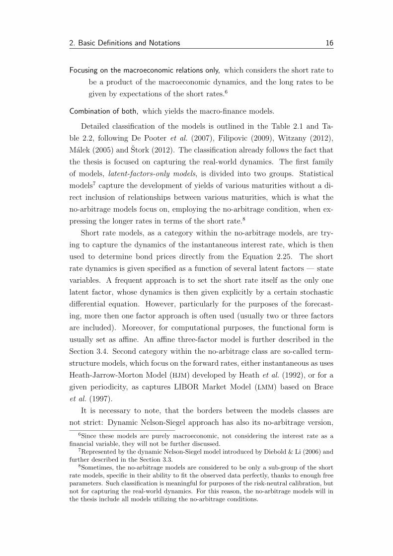
Moreover, the macro-finance models differ also in the character of the macroe-
conomic variables included. Two general approaches are possible: either ex-
plicit macro-variables time-series enter the model, or indices of key macroeco-
nomic areas, built for example by using Principal Component Analysis (PCA),
represent the macro-dynamics instead. This issue is further described in the
Chapter 4, when describing the data used for the practical analysis.
Table 2.2: Macro-Finance Models
Approach Factors’ Dynamics Time-Series Character
Affine model extension Non-structural: VARExplicitIndices
DSGE framework Structural: optimization Explicit
Nelson-Siegel extension Non-structural: VARExplicitIndices
Source: author’s own
In further chapters, the thesis will focus on a comparison of the performance
of various models, especially in terms of the estimation properties and the
forecasting ability. Two latent-factors-only models will be used, including both
the no-arbitrage approach represented by a three-factor affine model, and the
statistical dynamic Nelson-Siegel framework. Similarly, two related macro-
finance models will be introduced and their ability to beat the predictive power
of the latent-factors-only models will be tested —the macro-finance models will
be built as extensions of the affine and Nelson-Siegel latent-factors-only models.
In these models, only the explicit inclusion of the macroeconomic variables will
be considered.
2.4 Methodology
The thesis will continue in the following way: First, in the Chapter 3, the men-
tioned models will be described into a detail. When dealing with the dynamic
Nelson-Siegel framework, particular focus will be set on the possibilities to ob-
tain the optimal values of the parameters. Contrary, for the affine models, the
most challenging task will be to derive properly the discrete-time specification
of the model, following relevant literature and utilizing the fundamentals of the
financial mathematics and the stochastic calculus.
Second, after describing the data used for the analysis and splitting them

2. Basic Definitions and Notations 19
into training and testing samples, PCA will be used to reduce the dimensionality
of the yields. Afterwards, the models themselves will be estimated, using several
techniques:
� time series analysis, utilizing the Box & Jenkins (1970) methodology,
particularly the reduced-form VAR;
� Ordinary Least Squares (OLS) method;
� and numerical iterative methods.
Third, the estimations will be evaluated. The features of the estimations
themselves will be described, using Residual Sum of Squares (RSS) to compare
the models in terms of their ability to fit the observed values, and Impulse-
Response Function (IRF) to depict the qualitative properties of the estimations.
The estimations will be also used to construct predictions, and the forecasting
performance will be compared by calculating the total squared predictive error.
Finally, all the models will be re-estimated for a shorter data samples, and
the time development of the forecasting ability will be inspected. In this case,
the Root Mean Square Error (RMSE) will be used as the quantitative measure.
At the end, the results will be compared with outcomes of similar studies.
In the thesis, MATLAB and R-Studio are used when estimating the models
and producing the forecasts, as well as for construction of various charts.

Chapter 3
Description of Models
3.1 Factors and Principal Component Analysis
One of the biggest difficulties related to the yield curve modelling and fore-
casting seems to be the fact, that it is necessary to capture the dynamics of
many maturities (usually 10-15). This might be, due to the resulting over-
parametrization of a model, quite a problematic task. The common approach
is to model the dynamics of several latent (i.e. unobservable) factors, and de-
rive relations of the yields to these factors. For purposes of the financial assets
valuation, the task can be well simplified by calibrating a one-factor model,
typically Vasicek (1977) or Hull & White (1990) model. Since the dynamics
of rates of longer maturities are given by the no-arbitrage condition (applied
under a risk-neutral probability measure) in these cases, the model is able to
capture the dynamics using only one source of uncertainty – the short rate.
However, for purposes of a dynamic real-world analysis (as an opposite to
the risk-neutral pricing) and particularly forecasting, this approach might be
considered as inefficientRather than fitting the observed market situation, the
model should in this case also incorporate the exact relationship between the
yield curve shifts and changes of the factors driving these movements — since
various parts of the term structure have a different sensitivity to changes of
various underlying factors, it is necessary to allow multiple sources of the risk
to enter the models. It has been shown by Litterman & Scheinkman (1991)
that three factors are perfectly able to explain the dynamics of the whole yield
curve. The nature of these factors can be obtained by the PCA of yields, which
allows an elegant reduction of the dimension1 while setting a useful basis for
1It is implied directly by the nature of the PCA, that there does not exits any linear

3. Description of Models 21
building macro-finance models. The logic can be illustrated by the Figure 3.1.
Figure 3.1: Relationship of the Factors
Source: author’s own.
Representation of the entire yield curve by the three factors — principal
components (usually called Level, Slope and Curvature of the yield curve) —
can be considered as distinctively accurate. Litterman & Scheinkman (1991)
have shown that the three factors are able to explain more than 98% of the
total variance.2 The use of level, slope and curvature as the factors underlying
the yield curve movements is therefore beneficial in two ways:
� Only three variables are modelled, which solves the over-parametrization
problem.
� The new variables are tightly related to real macroeconomic and financial
factors driving the dynamics of the term structure.
The latter has been illustrated by Diebold & Li (2006), who have shown that
the level (the first component) is reflecting long-term inflation expectations,
whereas the slope (the second component) is connected to the real activity
and short-term inflation and growth expectations. The third component is
sometimes believed (Kollar 2011) to be related to the expectations of economic
growth and inflation in the medium time horizon.
Assuming the market is efficient, as defined by Fama (1970), market prices
(i.e. also bond yields ) should always capture all relevant available informa-
tion, including development of the macroeconomic variables. Consequently, for
purposes of the financial assets pricing, capturing dynamics of the latent fac-
tors (level, slope and curvature) is perfectly sufficient. However, such approach
does not include the particular relations of the macroeconomic variables and
transformation of the original variables incorporating more information (i.e. variance ofthe original data) than the first principal component, and a linear transformation with thetransformation vector orthogonal to the vector of the first transformation, which would beable to include more information than the second principal component, etc.
2A similar analysis will be performed also in the practical part of the thesis.

3. Description of Models 22
the term structure of interest rates. This can be a shortcoming for economic
subjects — typically central banks or governments — assessing an impact of
particular monetary or fiscal policy steps on the interest rates of various ma-
turities. This is where the macro-finance models are particularly useful, when
adding the macroeconomic variables directly into the models - their explicit
inclusion allows a simple analysis of the impact of monetary (or fiscal) policy
steps on the interest rates and its further propagation into the whole economy.
The difference between the latent-factors-only and the macro-finance models is
depicted by the Figure 3.2.
Figure 3.2: Inclusion of the Factors in the Models
Source: author’s own.
Four different models will be introduced in the following text, focusing on
their nature, derivation and an approach to their estimation and construction
of predictions.
Random walk will serve as a simple baseline, which the other models will be
assumed to outperform.
Dynamic Nelson-Siegel model, i.e. a model based on a specific utilization of the
Nelson-Siegel framework, will be estimated in two ways:
1. A simple dynamic version of the Nelson-Siegel representation of the
yield curve, including only the latent variables.
2. A macro-finance model explicitly including macro-variables into the
vector of factors driving the movements of the term structure of
interest rates.
Affine model, based on the no-arbitrage assumption, will be also built in two
forms, following the same logic:
1. An affine model including the three latent factors only.

3. Description of Models 23
2. And again its macro-finance extension with macro-variables included
in the vector of the factors — state variables.
3.2 Random Walk
To be able to assess the performance of both latent-factors-only and macro-
finance models, it is necessary to introduce a simple model serving as a baseline.
The yields of most maturities can be regarded as nonstationary, as will be shown
in the Section 4.1. For this reason, a random walk could be regarded as the most
simple baseline. Moreover, considering the random walk as a process the prices
are assumed to follow under the efficient market hypothesis (in compliance with
Fama 1965), testing the ability of other models to outperform the random walk
will implicitly create a naıve test of the market efficiency itself.3
The random walk (without a constant) can be written as:
rt (τ) = rt−1 (τ) + at,τ (3.1)
where at,τ represents a white noise process, i.e.
E [at,τ ] = 0
var [at,τ ] = σ2a,τ
cov [at,τ , as,τ ] = 0 for s 6= t
Predictions resulting from the random walk are very simple to obtain - they
are equal to the latest observation:
E [rt+1 (τ)] = E [rt (τ)] + E [at+1,τ ] = rt (τ) (3.2)
3.3 Dynamic Nelson-Siegel Approach
Basic Description
A pivotal work in this area is Diebold & Li (2006). Authors try to react on poor
results of no-arbitrage models in terms of predictive performance, assuming that
3It is, however, necessary to note, that the author is not aiming at proving or refusing thehypotheses of Eugene Fama, which are definitely going far behind the extent of the thesis.

3. Description of Models 24
leaving the no-arbitrage restrictions (used in the Section 3.4 when constructing
the affine model) may lead to more accurate forecasts.
The first step to take when building the model is to describe the basic
Nelson-Siegel framework, based on the work of Nelson & Siegel (1987). Authors
offered a statistical approach to the estimation of the term structure of interest
rates, which quickly became popular, mainly for its relative simplicity. The
main building block of the framework is a representation of the yield curve as
a function of the maturity in the following form:
r (τ) = β1 + β2
(1− e−λτ
λτ
)+ β3
(1− e−λτ
λτ− e−λτ
)(3.3)
where τ = T − t represents the time to maturity and β1, β2, β3 and λ are the
parameters to be estimated. Later, the Equation 3.3 was extended by Svensson
(1994), including an extra term to enhance the flexibility of the function when
fitting the term structure; however, the original form is often considered to be
flexible enough, which will be assumed also henceforth. The resulting estimated
term structure does not fit the observed values exactly — consequently the
bond prices implied by the Nelson-Siegel estimation may slightly deviate from
the observed ones. However, the specific exponential form of the function as
defined by the Equation 3.3 ensures substantial flexibility, which makes the
approach attractive.4
The three indexed beta parameters are of a special interest,5 since they can
be (and often are) considered as representatives of the main characteristics of
the term structure of interest rates — the latent factors:
� β1 is common for all maturities, so it represents the level of the term
structure.
� The expression directly following β2 (i.e. its factor loading) is decreasing
with growing maturity (approaching 1 with the maturity decreasing to
0, respectively going to 0 with the maturity approaching +∞), assuming
λ is positive. Positive β2 therefore implies short maturities being bigger
than the long ones and vice versa — and β2 can be therefore interpreted
as a negative slope of the term structure. The development of the β2
4Compared to the restricted ability of Vasicek (1977) or Cox et al. (1985) models to fitthe observed term structure of interest rates (Malek 2005).
5Whereas λ is set in order to ensure either an optimal shape of the yield curve or the bestfit of the original and model-implied yields, as will be described below.

3. Description of Models 25
factor loading, for maturities between 0 and 15 and various values of
lambdλ a, is outlined by the Figure 3.3
Figure 3.3: Slope - Factor Loading for Various λ Values
0 1 2 5 10 20 30
0
0.1
0.2
0.3
0.4
0.5
0.6
0.7
0.8
0.9
1
maturity
fact
or lo
adin
g
0.10.20.512510100
Source: author’s own.
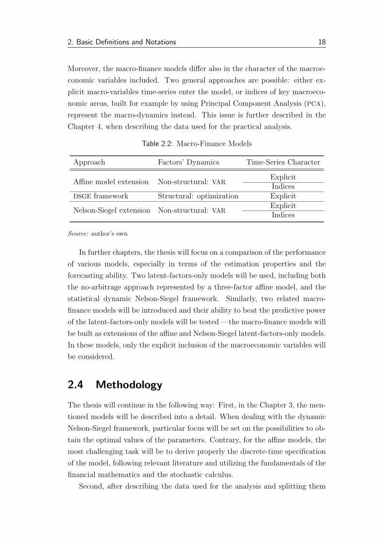
� The β3 factor loading is positive for positive λ and approaches zero for
maturities reaching either 0 or +∞. The maturity, for which the factor
loading is in its maximum, depends on the value of λ: with growing λ,
the maturity in which the maximum is obtained is decreasing. Conse-
quently, the third expression can be considered as a location of a ”hump”
in the term structure, whereas the β3 itself represents extent of the cur-
vatures. Setting the λ positive, yields of medium maturities will be rel-
atively higher than the short or long rates. Possible values of the factor
loading are illustrated by the Figure 3.4.
The interpretation of the β parameters is very close to the interpretation
of the first three principal components of the yield curve, as explained above.
Nelson-Siegel parametrization consequently offers an elegant and simple ap-
proach how to use the benefits of the Litterman & Scheinkman (1991) findings
in practice. The favourable properties of the Nelson-Siegel representation con-
firm also Diebold & Li (2006), when noting that this approach keeps the key
properties of the term structure, mostly in terms of implied forward rates and
the ability to fit well many possible shapes of the yield curve observed at the
market.
When fitting the yield curve on the observed data, one of the frequent
approaches is to estimate separately the β parameters, using OLS and assuming
3. Description of Models 26
Figure 3.4: Curvature - Factor Loading for Various λ Values
0 1 2 5 10 20 30−0.05
0
0.05
0.1
0.15
0.2
0.25
0.3
maturity
fact
or lo
adin
g
0.10.20.512510100
Source: author’s own.
the λ parameter to be fixed, then evaluate the accuracy of the fit, and find such
a λ maximizing the accuracy (can be measured by R-square of the OLS or by
the information criterion of the model).
Dynamic Version and Macro-Finance Extension
Diebold & Li (2006) introduced a new view on the Nelson-Siegel function.
Considering the β parameters as time-varying latent factors, the dynamics of
the yield curve can be derived from the dynamics of these latent factors. The
model is described by two equations (Diebold et al. 2006):
rt (τ) = β1,t + β2,t
(1− e−λτ
λτ
)+ β3,t
(1− e−λτ
λτ− e−λτ
)+ εr,t (τ) (3.4)
βt = α+ Γβt−1 + εβ,t (3.5)
where βt is a 3× 1 vector consisting of βt,1, βt,2 and βt,3; the scalar error terms
of the yields εr,t (τ) are forming a m × 1 vector error term εr,t (where m is
number of maturities τ in the sample), which is believed to follow N (0,Σr)
distribution with Σr being a m ×m covariance matrix; εβ,t is a 3 × 1 vector
error term related to the stochastic process of βt, assumed to follow aN (0,Σβ)
distribution (with Σβ of a dimension 3 × 3), and α and Γ are a 3 × 1 vector,
respectively a 3× 3 matrix of parameters.
The Equation 3.5 is simply a representation of a three-dimensional VAR
process with one lag, which can be considered as the most simple way how to
3. Description of Models 27
capture the development of βt, and will be used also in the thesis. One benefit of
the VAR model used in the Equation 3.5 is that the construction of the resulting
macro-finance model is very simple. The 3 × 1 vector of latent variables βt
including the latent factors level, slope and curvature can be enriched by a k-
dimensional vector θt including k macroeconomic variables, to form a (3 + k)×1
vector (henceforth denoted ηt). The original three-dimensional VAR process
will be modified into a (3+k)-dimensional (following Diebold et al. 2006):
[βt
θt
]= µ+ Φ
[βt−1
θt−1
]+ εη,t (3.6)
ηt = µ+ Φηt−1 + εη,t (3.7)
where µ, Φ and εη,t are similar to α, Γ and εβ,t, differing only in their dimen-
sions.
The macro-variables included in the vector θ do not influence the yields
directly (i.e. they are not included in the Equation 3.4), but only through
the impact on the development of the latent β factors, which then govern the
yields themselves. The macroeconomic variables are considered as exogenous,
and the macro-finance relationship is therefore only one-sided6, lacking the
reverse causality in the direction from the interest rates to the macroeconomic
variables. This simplification can reduce the performance of the model, as
a consequence of an omission of some transition channels, nevertheless the
simplicity of resulting model can be beneficial in terms of a robustness and a
good estimation performance, especially when focusing on the predictive power.
Estimation and Forecasting
Diebold & Li (2006), or similarly Kollar (2011) for the Czech yield curve,
proceed in the following way: First, for each period, the Nelson-Siegel function
is fitted on the observed maturities — i.e. the parameters of the Equation 3.4
are estimated for each period separately; β coefficients are allowed to vary,
whereas λ is kept fixed. Afterwards, the estimated β parameters, representing
the latent factors — level, slope and curvature — enter the model capturing
their dynamics: a reduced-form VAR model defined in the Equation 3.5 is
estimated, using a least-squares method. After an evaluation of the error term
6Which will be followed also in all other models included in the thesis
3. Description of Models 28
of the model in terms of diagnostic tests, properties of the estimated model can
be analysed, typically using IRF, to comment on the dynamics implied by the
model.
Different approach present Diebold et al. (2006), using the very nature of
the described model — it is a typical representative of a State-Space model
in the most basic form. Observed values are determined by unobservable (la-
tent) factors, which are following VAR(1) process. Following the methodology
of these models (for example in Pichler 2007), the Equation 3.4 can be called a
measurement equation, since it represents the process how the latent factors are
related to the measurable variables (yields); consequently, εr,t is a measurement
error. The Equation 3.5 is a state (transition) equation, which describes be-
havior of the latent variables, and includes the state equation errors εβ,t. Since
the relationship is linear, the two steps can be jointly estimated by Kalman
filter (Kalman 1960), which is a special method for constructing and using the
likelihood function in the State-Space models framework, even when the least
squares methods are not applicable (Pichler 2007).
The macro-finance extension is then constructed rather easily. The β pa-
rameters enter the Equation 3.6 instead of the original one, regardless to which
of the two approaches to the estimation is used - no change of the estimation
methods is necessary. A shock into a macroeconomic variable (either external
or resulting from a policy-making process) is directly (with a one-period lag)
propagated into the other macroeconomic variables and simultaneously into
the latent factors, which can be well depicted by the IRF. The latent factors
then directly determine the new shape of the yield curve.
After the models are estimated, the forecasts can be constructed by step-by-
step iterating the β (or η in the macro-finance model) vector through the transi-
tion equation 3.5 (respectively 3.7), utilizing the fact that E [εβ,t] = E [εη,t] = 0.
The forecasts of the yields themselves then result from the measure Equa-
tion 3.4.
It is useful to describe, returning to the start of the estimation, how to
obtain the fixed λ parameter. Since the parameter determines the maturity in
which the curvature factor is maximal (see Figure 3.4), Diebold & Li (2006)
simply argue the optimal λ should ensure the largest curvature for maturities
2-3 years, which are, according to the authors, the most appropriate from the
empirical point of view. More specifically, the authors find such a λ maximizing
the curvatureβ3 factor loading for 30 months maturity.
However, because the data scope analysed in the thesis includes quite vari-
3. Description of Models 29
able shapes of the yield curve (particularly after the 2009 crisis), as well as
a different ”hump” location for different periods, the approach to set λ as
mentioned above could be considered as unreasonable. Instead, λ may be de-
termined so that it ensures an optimal fit of estimated and observed values.
The procedure can be described in the following way:
1. An arbitrary λ1 is chosen.
2. For each period t, the β vector is obtained by a simple OLS method, using
the maturities in the given period as the observations:
βt =(XTX
)−1XTrt (3.8)
where:
βt =
β1,t
β2,t
β3,t
,
rt =
rt (τ1)
rt (τ2)...
rt (τm)
,
X =
1 1−e−λ1τ1
λ1τ11−e−λ1τ1
λ1τ1− e−λ1τ1
1 1−e−λ1τ2
λ1τ21−e−λ1τ2
λ12− e−λ1τ2
......
...
1 1−e−λ1τm
λ1τm1−e−λ1τm
λ1τm− e−λ1τm
with m = number of maturities in the sample.
3. Then, the difference between the estimated and observed values (residuals
et) is calculated as:
et = rt − rt = rt −Xβt (3.9)
4. Finally, returning to λ, the numerical methods are used to find its optimal
value, i.e. minimizing the residual sum of squares (RSS) over all periods:
minλ
n∑t=1
etTet (3.10)
where n is the number of the periods included in the sample.

3. Description of Models 30
To conclude, there will be multiple models belonging to the dynamic Nelson-
Siegel family estimated in the Section 4.3, and their results will be compared.
The different approaches are captured by the Table 3.1.
Table 3.1: Dynamic Nelson-Siegel Models
model name type λ setting
NS-L-A latent-factors-only curvature locationNS-L-B latent-factors-only optimal fitNS-M-A macro-finance curvature locationNS-M-B macro-finance optimal fit
Source: author’s own
3.4 Affine Model
Basic Description
Apart from the dynamic Nelson-Siegel approach, model introduced in this sec-
tion is using no-arbitrage assumption when determining the bond prices and
the term structure of interest rates itself. As explained in the previous chapter,
under the risk-neutral measure, the value of a bond is given directly by the
expected development of the instantaneous (short) rate:
Pt(τ) = EQ
[e−
∫ t+τt rsds
](3.11)
where EQ denotes the expectations under the risk-neutral measure. To be
able to explain the dynamics of the bond prices (and hence the whole term
structure) in time, it is necessary (as notes Piazzesi 2009) to solve two related
issues:
� to capture the dynamics of the short rate, and
� to link risk-neutral and real probability measures.
To deal with both tasks, an affine model will be used, as one of the most
frequent approaches to the interest rate modelling. Following the work of Duffie
& Kan (1996), the term structure model is called affine if the dynamics of the
short rate rt is an affine function of the state variables:
rt = a0 + aT1Lt (3.12)
3. Description of Models 31
where Lt is a l-dimensional vector of the state variables (or latent factors), a0
is a scalar parameter and a1 is a l-dimensional vector of parameters. In case
l = 1, the a one-factor (usually short rate) model is obtained, otherwise it can
be called as a multi-factor model. Using a simple example of Vasicek (1977)
model, a0 = 0, l = 1, a1 = 1 and the only latent factor is consequently the short
rate itself, whose evolution is then given by a particular stochastic differential
equation.
More generally, for both one-factor and multi-factor models, the dynamics
of Lt is given by the following equation:
dLt = K1 (k2 −Lt) dt+ ΣLStdW t (3.13)
where K1 and ΣL are l× l matrices and k2 is a l× 1 vector of parameters, and
St is a diagonal l × l matrix with elements being a function of Lt. Moreover,
W t is a l-dimensional Brownian motion, assuming the model is described still
under the risk-neutral measure Q. The diagonal elements (noting Sii the i-th
diagonal element) of the St matrix can be expressed in the form:
Sii =√b1,i + bT2,iLt (3.14)
Where b1,i is a scalar parameter and b2,i is a l × 1 vector of parameters.
The affine models further assume there are certain restrictions on the par-
ticular form of the Equation 3.13 (which are outlined for example in Malek
2005 for a one-factor model). Duffie & Kan (1996) show that in that case,
price of a bond can be expressed as an exponentially affine function in terms
of the state factors:
Pt(τ) = eB1(τ)+BT2 (τ)Lt (3.15)
Where B1(τ) and B2(τ) are deterministic functions of a maturity, i.e. for a
given maturity τ , they represent coefficients (a scalar and a vector)7. Moreover,
the functions can be obtained directly by solving a set of ordinary differential
equations (for a one-factor model again in Malek 2005).
7Sometimes, there is used a negative sign before B2(τ) term in the Equation 3.15, butthe results must be necessarily equivalent regardless to the chosen form.

3. Description of Models 32
Utilizing the Equation 2.11, the interest rates (for the maturity τ > 0) can
be expressed, after plugging for Pt(τ) from the Equation 3.15, in the form:
rt(τ) = − lnPt(τ)
τ= −B1(τ)
τ− B
T2 (τ)Ltτ
= C1(τ) +CT2 (τ)Lt (3.16)
It is important to remind, that all the above-defined parameters are related
to the dynamics under the risk-neutral measure. Conversion of the risk-neutral
measure may be performed using the already mentioned Girsanov theorem,
which is defined for example in Shreve (2004). Assuming λ is a l-dimensional
vector of market prices of risk8 related to the l state variables, the Girsanov
theorem implies that
dW t = dW t + λtdt (3.17)
where W t is a Brownian motion under the real probability measure. Then, the
Equation 3.13 can be, after plugging in for expression dW t from Equation 3.17,
rewritten under the real probability measure as
dLt = K1 (k2 −Lt) dt+ ΣLStλtdt+ ΣLStdW t (3.18)
Duffie & Kan (1996) assume, that the market price of risk is a function of the
state variables volatility, specifically:
λt = Sth (3.19)
where h is a l × 1 vector of constant parameters. After plugging into the
Equation 3.18 and using the definition of the St matrix, the dynamics of the
state variables modifies in the following way:
dLt = K1 (k2 −Lt) dt+ ΣLS2thdt+ ΣLStdW t (3.20)
dLt = M 1 (m2 −Lt) dt+ ΣLStdW t (3.21)
where M 1 and m2 are of the same dimensions as K1 and k2, and are directly
given by K1, k2, ΣL, h and parameters b1,i and b2,i from the St matrix, as
shows for example Kladıvko (2011).
8λ symbol has been used in a different context in dynamic Nelson-Siegel models, the no-tation is though not adjusted in order to comply with the common notation in the literature.
3. Description of Models 33
Consequently, after fitting the model under the risk-neutral measure, the
real-world behavior of the latent factors can be, thanks to the mentioned specific
relation of the market prices of risk and latent factors, obtained quite easily.
However, for example Duffee (2002) considers this restriction as too strict, and
offers an affine model allowing more realistic dynamics of the market price of
risk.
Discrete-Time Specification
Similarly to other studies, it may be convenient to capture the whole dynamics
in a discrete time. Simultaneously, following Ang & Piazzesi (2003), the general
affine model as described above will be given a specific form, allowing to obtain
the parameters for both Equation 3.16 and dynamics of the latent factors. In
the model, three latent factors are used, which is perfectly enough (see the
discussion about Litterman & Scheinkman (1991) findings included above).
First, it is necessary to specify the dynamics of the underlying latent factors
Lt, i.e. a discrete-time analogy to the equation Equation 3.13. Being still
inspired by Ang & Piazzesi (2003), the VAR process is used in this respect.
Including only one lag into the VAR equation, the resulting model can be truly
seen as an analogy of the continuous-time process (admitting that the following
notation is not an exact discrete approximation, but rather an intuition)9:
∆Lt = K1 (k2 −Lt) ∆t+ ΣL∆W t
Lt+1 = Lt +K1 (k2 −Lt) (t+ 1− t) + ΣL
(W t+1 − W t
)Lt+1 = K1k2 + (1−K1)Lt + ΣLεt+1
Lt+1 = γ0 + Γ1Lt + ΣLεt+1 (3.22)
where γ0 is a l×1 vector and Γ1 represents a l×l matrix of parameters, whereas
εt+1 is a l-dimensional random term assumed to follow N(0, I). Moreover, ΣL
term is in this case a l×l matrix of coefficients. It is also necessary to determine
the specific dynamics of the market price of risk. The l-dimensional vector λt
9In the model, the specific form of the volatility as announced by Duffie & Kan (1996) anddescribed above is not utilized. For this reason, the volatility coefficients ΣLSt are replacedin the notation simply by ΣL in order to simplify the functional form, keeping in mind thatthe ΣL term is different in both cases.

3. Description of Models 34
is here assumed to be affine in the state variables:
λt = λ0 + λ1Lt (3.23)
with λ0 being a l-dimensional vector and λ1 being a l× l matrix of parameters.
The discrete-time specification influences also the way the bond price is
expressed in terms of expectations under the risk-neutral measure. In the
discrete time, the bond price may be defined, analogically to the Equation 3.11,
looking one period forward:
Pt(τ + 1) = EQ
[Pt+1(τ)
ert
](3.24)
Obviously, it is necessary to convert the risk-neutral measure into the real-
world. This can be done via the Radon-Nikodym derivative, which is, together
with the Girsanov theorem, one of the basic building blocks of the risk-neutral
dynamics. Following steps are based mostly on Ang & Piazzesi (2003), Gisiger
(2010), Haugh (2010), Shreve (2004) and Malek (2005), employing the basics
of the stochastic calculus and the risk-neutral probability approach.10
The Radon-Nikodym derivative Z of the risk-neutral measure Q with re-
spect to real-world measure P can be defined as:
Z =dQ
dP(3.25)
It is further possible to define a Radon-Nikodym process Zt, which is assumed
to be a martingale under the P -measure:
Zt = EP [Z|Ft] (3.26)
where Ft is a filtration.
Consequently, using conditional expectations and employing the definition
of Z, following holds for any Ft+1-measurable random variable Xt:
EQ [Xt+1|Ft] =EP[dQdPXt+1|Ft+1
]EP[dQdP|Ft] =
EP [Zt+1Xt+1|Ft+1]
Zt(3.27)
The discrete-time dynamics of the Radon-Nikodym proces Zt is specified as a
10Since a complex description of the stochastic calculus and the risk neutrality issues wouldrequire a far larger space than possible to use in the thesis, only the most relevant facts andissues will be mentioned, referring to the included literature in the other cases.
3. Description of Models 35
log-normal process (Ang & Piazzesi 2003)
Zt+1 = Zte− 1
2λTt λt−λTt εt+1 (3.28)
The last assumption is a definition of a nominal pricing kernel Mt+1:
Mt+1 = e−rtZt+1
Zt(3.29)
Mt+1 = e−rt−12λTt λt−λTt εt+1 (3.30)
The second equation has been obtained by plugging in for Zt+1 from the Equa-
tion 3.28. The pricing kernel (called also a stochastic discount factor) is a key
(random) variable used to price (discount) the nominal assets in economy - un-
der the real probability measure. Using a naıve intuition, the pricing kernel may
be seen as a representation of the denominator from the Equation 2.20. In other
words, returning to the very beginning of the thesis, the general thought of an
individual required yield yreq as introduced in Equation 2.1, which depends on
a risk-free time factor ρ, an expected inflation E [π] and a risk premium ξ, is
explicitly formulated by the Equation 3.30, including the risk-free rate rt and
the market price of risk λt as exact specifications of (ρ+ E [π]) and ξ.
The specification of the pricing kernel as defined above, as well as the men-
tioned intuition behind, is implying a recursive equation for bond prices:
Pt(τ + 1) = EP [Mt+1Pt+1(τ)|Ft] (3.31)
which can be proven directly by merging equations 3.24, 3.27 and 3.29, replacing
Xt and Xt+1 by Pt(τ + 1) and Pt+1(τ):
Pt(τ + 1) = EQ
[Pt+1(τ)
ert
∣∣∣∣Ft]= EP
[Zt+1Pt+1(τ)
ertZt
∣∣∣∣Ft]= EP [Mt+1Pt+1(τ)|Ft]
Obviously, the Equation 3.31 is the representation of the Equation 3.24 under
the real probability measure, which is exactly what was aimed to obtain.
The only variable determining (recursively) the bond price Pt(τ+1) is hence
the pricing kernel Mt+1, specified by the Equation 3.30. On the other hand, the
pricing kernel is, apart from the random term εt+1, driven by the development
3. Description of Models 36
of the short rate rt and the market price of risk λt. Since both these variables
are expressed as an affine function of the latent factors Lt (see equations 3.12
and 3.23), the bond price itself can be obtained as a function of the latent
factors only (apart from the maturity).
Moreover, Ang & Piazzesi (2003) show, that the functions Pt(τ + 1) =
fτ (Lt), which are recursively defined for bonds of growing maturities, are ex-
ponentially affine, which proves that the model belongs to the affine class of
models. The functions B1(τ) and B2(τ) from the Equation 3.15 themselves
can be then shown (see Appendix A. from Ang & Piazzesi (2003) for a proof)
to be in the following recursive form:
B1(1) = −a0B2(1) = −a1 (3.32)
and
B1(τ + 1) = B1(τ) +BT2 (τ) (γ0 −ΣLλ0) +
1
2BT
2 (τ)ΣLΣTLB2(τ)− a0
BT2 (τ + 1) = BT
2 (τ) (Γ1 −ΣLλ1)− aT1 (3.33)
where the coefficients are those used in the equations 3.12, 3.22 and 3.23.
The interest rates can be the simply expressed as affine functions of the
latent factors, with C1(τ) and C2(τ) obtained simply from B1(τ) and B2(τ),
as defined in the Equation 3.16. Consequently, the whole model can be written
as
rt(τ) = C1(τ) +CT2 (τ)Lt + εr,t(τ) (3.34)
Lt = γ0 + Γ1Lt−1 + ΣLεt (3.35)
where the inclusion of εr,t(τ), assumed to be N(0, σt(τ)) distributed, is moti-
vated by allowing a possibility that there may be a random disturbances in the
relation of the latent factors and the interest rates.
Macro-Finance Extension
As point out De Pooter et al. (2007), the equations 3.34 and 3.35 are very
similar to the equations 3.4 and 3.5. This allows to give them the same inter-
pretation: they can be considered as measure and transition equations forming

3. Description of Models 37
a simple state-space model. Moreover, the transformation of the model, in-
cluding macroeconomic variables, is based on the same idea: the l-dimensional
vector Lt in the Equation 3.35 is extended by k macroeconomic variables, form-
ing a (l + k)-dimensional vector V t. However, being inspired by the approach
used by Ang & Piazzesi (2003), there is one important difference compared
to the dynamic Nelson-Siegel approach: the macroeconomic variables influence
the dynamics of the yields directly. In other words, macro-factors enter also the
Equation 3.34, whereas in the case of the previous group of model, the Equa-
tion 3.4 remained unchanged, with the macro-variables influencing the yields
only indirectly through the joint dynamics with the latent factors, as capture
equations 3.6 or 3.7.
The whole affine macro-finance model can be written in the form:
rt(τ) = C1(τ) + CT2 (τ)V t + εr,t(τ) (3.36)
V t = γ0 + Γ1V t−1 + ΣMεt (3.37)
where
V t =
[Lt
θt
](3.38)
with θt being the k-dimensional vector of added macroeconomic variables, εt
being a (k + l)-dimensional random error assumed to be N(0, I) distributed,
and other vectors and matrices being the extended versions of similar terms
from the equations 3.34 and 3.35. When compared to the latent-factors-only
form, different will be not only the VAR parameters γ0, Γ1 and ΣM , but since
they enter the Equation 3.33, also C1(τ) and C2 will differ.
Estimation and Forecasting
For the estimation of the models, an approach following Ang et al. (2006) and
De Pooter et al. (2007) will be used. Focusing on the latent-factors-only model,
the estimation includes several steps:
� First, the latent factors will be assumed to be represented by the first
three principal components of the yields. Based on these variables, the
parameters of theEquation 3.35 will be estimated - γ0 and Γ1 will be
3. Description of Models 38
obtained by the least squares method, and ΣL will be calculated from
the covariance matrix of the residuals, using Choleski decomposition.
� Second, the parameters a0 and a1 from Equation 3.12 will be calculated
by OLS, using the shortest observed yield as a proxy for the short rate.
� Last step is to obtain values of λ0 and λ1 such that the resulting yields
from the Equation 3.34 are as close to the observed yields as possible.
That means that after iterative plugging in for λ0 and λ1 into the Equa-
tion 3.32, using values of other parameters obtained from the previous
steps, B1 and B2 are calculated recursively for each maturity, as well as
C1 and C2. The fitted yields are then obtained from:
rt(τ) = C1(τ) + CT
2 (τ)Lt (3.39)
and λ0 and λ1 will result from:
minλ0,λ1
n∑t=1
m∑i=1
[rt(τi)− rt(τi)]2 (3.40)
where m is a number of maturities and n a number of periods included
in the sample.
For the macro-finance version, the estimation process will be exactly iden-
tical, using the vector V t instead of Lt. Finally, forecasts of the yield curve
may be constructed, using the estimated values of parameters. First, by itera-
tive plugging in for Lt (or V t) into an estimation of the Equation 3.35 (3.37),
forecasts of Lt+1 (V t+1) will be obtained. The values of yields predicted by the
model then result directly from an estimation of the Equation 3.34 (3.36).

Chapter 4
Estimation
4.1 Data
Interest Rates Data
In this thesis, U.S. zero-coupon bond yields are used to form the term structure
data, similarly to other studies. The data include end-of-month yields for bonds
of 10 maturities1: American Government Bills of three and six months and one
year maturities, US Notes (2, 3, 5, 7 and 10 years) and, finally, 20- and 30-years
US Government Bonds. In the period between February, 2002 and February,
2006, there were no data released for the longest maturity bonds (30Y), but
the U.S. Treasury offers calculated adjustments allowing to obtain data for the
30-years US bonds by extrapolating the 20-years bonds yields (U.S. Treasury
2014), which is used also in the thesis.
The data are obtained from the FRED (2014) database. The monthly
frequency was chosen to comply with the frequency of the macroeconomic vari-
ables, for which the monthly periodicity is the most frequent possible, as will
be discussed below. The data are already obtained in terms of yields (per
annum). More specifically, the FRED (2014) database uses constant maturity
rates, which are calculated by U.S. Treasury by interpolating the yield curve for
the non-inflation-indexed Treasury securities2. Approaches to the yield curve
1Originally, 11 maturities were included into the analysis, adding also one-month U.S.Bills; however, restricted availability of the data for this maturity before year 2001 resultedin a weaker performance of the models, and moreover, originally analysed period became tooshort to allow the comparison of the performance of the models under different macroeco-nomic conditions.
2The issue of obtaining the constant maturity rates is described into the more detail inthe footnotes at the end of FED (2014).

4. Estimation 40
construction from the available data is theoretically described in the Chapter 2,
and since it is not in the centre of attention of the thesis, the interest rates data
are used passively, without further discussion or adjustments.
The data include period starting in October, 1993 and ending in February,
2014, which covers 245 observed end-of-month dates. This particular period
was chosen for a few reasons:
� The period is long enough to provide the data allowing to use the chosen
modelling techniques.
� Simultaneously, the period is short enough to ensure it is eligible to as-
sume there were no systematic changes in terms of a theoretical function
describing the optimal reaction of the economic subjects on the economic
conditions, which is necessary for the stability of the macroeconomic re-
lationships, as requires the famous Lucas (1976) Critique. This fact is
very important particularly for the behavior of the central bank, which
can be assumed to operate under the inflation targeting monetary policy
paradigm during the whole period.
� Moreover, the economic conditions themselves have been changing during
the period, including both periods of economic expansions and shrinkages.
This allows to compare the performance of the models in various parts of
the business cycle.
The range of data will be split into a training sample, containing the data
until the end of 2012 (231 periods), and a testing sample including remaining
14 months. In further data analysis, only the training sample will be used,
and based on it, the models will be estimated and evaluated in terms of the
estimation properties. The testing sample will be reintroduced in the Chap-
ter 5, when will be used for an evaluation of the forecasting performance of the
models.
Afterwards, the same data will be the used again, estimating the models
on a shorter sample and rolling the estimation-forecasting process through the
whole data range. This facilitates comparison of the forecasting ability of the
models in different periods, as it can be expected that the benefit of adding the
macro-variables will vary with changing economic situation.
It is useful to outline the development of the term structure of interest rate
during the in-sample period 1993-2012. Figures 4.1 and 4.2 illustrate the key
shapes of the yield curve of the U.S. Government Bond yields in this period.
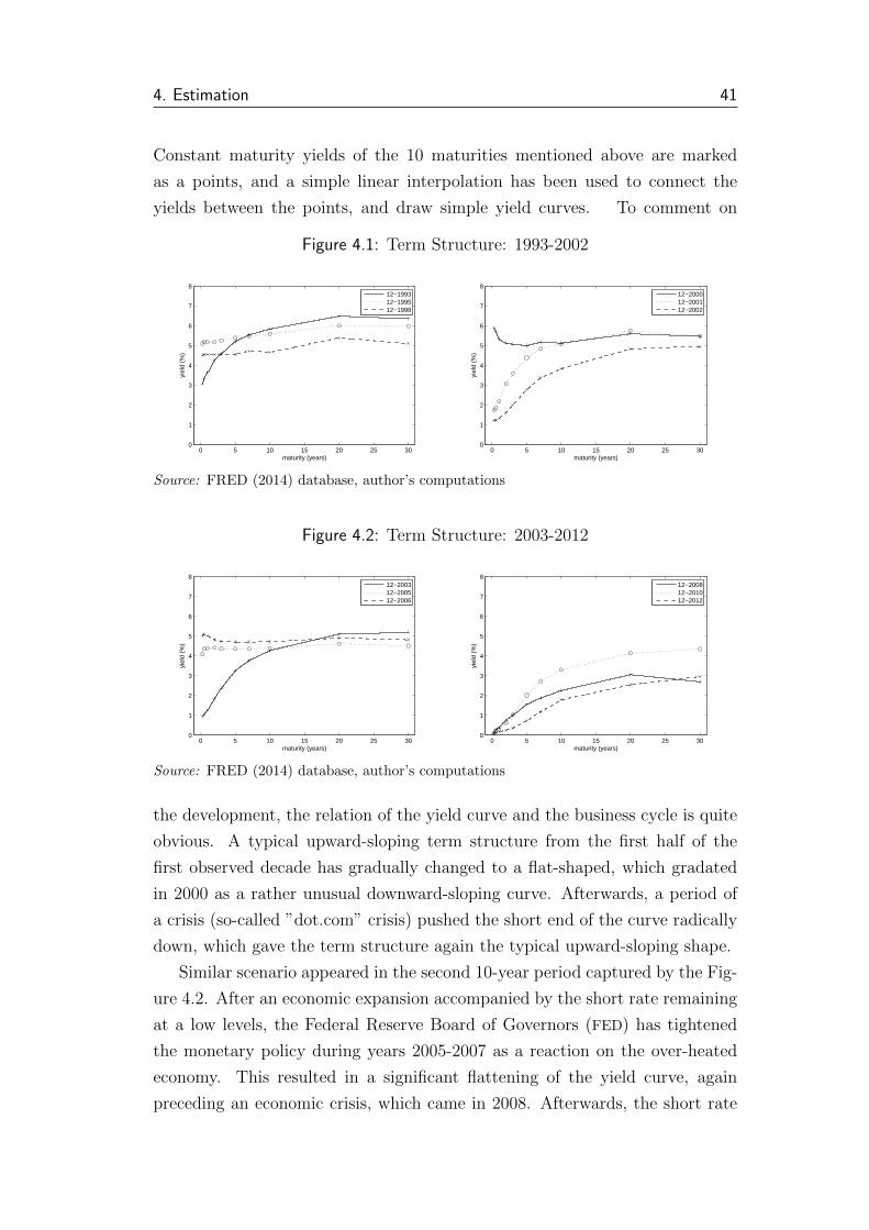
4. Estimation 41
Constant maturity yields of the 10 maturities mentioned above are marked
as a points, and a simple linear interpolation has been used to connect the
yields between the points, and draw simple yield curves. To comment on
Figure 4.1: Term Structure: 1993-2002
0 5 10 15 20 25 300
1
2
3
4
5
6
7
8
maturity (years)
yiel
d (%
)
12−199312−199512−1998
0 5 10 15 20 25 300
1
2
3
4
5
6
7
8
maturity (years)
yiel
d (%
)
12−200012−200112−2002
Source: FRED (2014) database, author’s computations
Figure 4.2: Term Structure: 2003-2012
0 5 10 15 20 25 300
1
2
3
4
5
6
7
8
maturity (years)
yiel
d (%
)
12−200312−200512−2006
0 5 10 15 20 25 300
1
2
3
4
5
6
7
8
maturity (years)
yiel
d (%
)
12−200812−201012−2012
Source: FRED (2014) database, author’s computations
the development, the relation of the yield curve and the business cycle is quite
obvious. A typical upward-sloping term structure from the first half of the
first observed decade has gradually changed to a flat-shaped, which gradated
in 2000 as a rather unusual downward-sloping curve. Afterwards, a period of
a crisis (so-called ”dot.com” crisis) pushed the short end of the curve radically
down, which gave the term structure again the typical upward-sloping shape.
Similar scenario appeared in the second 10-year period captured by the Fig-
ure 4.2. After an economic expansion accompanied by the short rate remaining
at a low levels, the Federal Reserve Board of Governors (FED) has tightened
the monetary policy during years 2005-2007 as a reaction on the over-heated
economy. This resulted in a significant flattening of the yield curve, again
preceding an economic crisis, which came in 2008. Afterwards, the short rate

4. Estimation 42
dropped again, making the term structure largely upward sloping. The severity
of the crisis have caused the longest rates to decrease gradually, however the
upward-sloped shape has remained until the end of the observed (in-sample)
period.
The development of the term structure dynamics can be illustrated also by
the Figure 4.3 including time series of yields of maturity 3 months (a proxy for
the short rate), 3 years, 10 years and 30 years (long rate).
Figure 4.3: Yields Time Series
12−1994 12−1997 12−2000 12−2003 12−2006 12−2009 12−20120
1
2
3
4
5
6
7
8
time
yiel
d (%
)
3M 3Y10Y30Y
Source: FRED (2014) database
The graphic representation suggests for nonstacionarity of the yields, which
can be supported by the Autocorrelation Function (ACF) and the Partial Au-
tocorrelation Function (PACF) of the yields (the maturities 3M, 3Y, 10Y and
30Y again chosen as representatives), as shows the Figure 4.4. However, re-
turning to the Figure 4.3, it seems that for the longer maturities, a linear
deterministic trend can be identified. This is proven by using the Augmented
Dickey-Fuller (ADF) test, with a linear trend and a constant.The null hypoth-
esis is a non-stationarity in this case. Results are included in the Table 4.1:
whereas the non-stationarity could not be rejected for the short and medium
maturities, opposite holds for the longest maturity, which is, according to the
test, clearly stationary (assuming a presence of the linear trend).
The yields are also highly correlated, with the correlation gradually de-
creasing for opposite parts of the yield curve. A reduced correlation matrix,
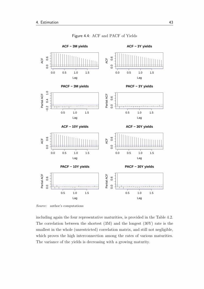
4. Estimation 43
Figure 4.4: ACF and PACF of Yields
0.0 0.5 1.0 1.5
0.0
0.6
Lag
AC
F
ACF − 3M yields
0.5 1.0 1.5
−0.
20.
41.
0
Lag
Par
tial A
CF
PACF − 3M yields
0.0 0.5 1.0 1.5
0.0
0.6
Lag
AC
F
ACF − 3Y yields
0.5 1.0 1.50.
00.
6
Lag
Par
tial A
CF
PACF − 3Y yields
0.0 0.5 1.0 1.5
0.0
0.6
Lag
AC
F
ACF − 10Y yields
0.5 1.0 1.5
0.0
0.6
Lag
Par
tial A
CF
PACF − 10Y yields
0.0 0.5 1.0 1.5
0.0
0.6
Lag
AC
F
ACF − 30Y yields
0.5 1.0 1.5
0.0
0.6
Lag
Par
tial A
CF
PACF − 30Y yields
Source: author’s computations
including again the four representative maturities, is provided in the Table 4.2.
The correlation between the shortest (3M) and the longest (30Y) rate is the
smallest in the whole (unrestricted) correlation matrix, and still not negligible,
which proves the high interconnection among the rates of various maturities.
The variance of the yields is decreasing with a growing maturity.
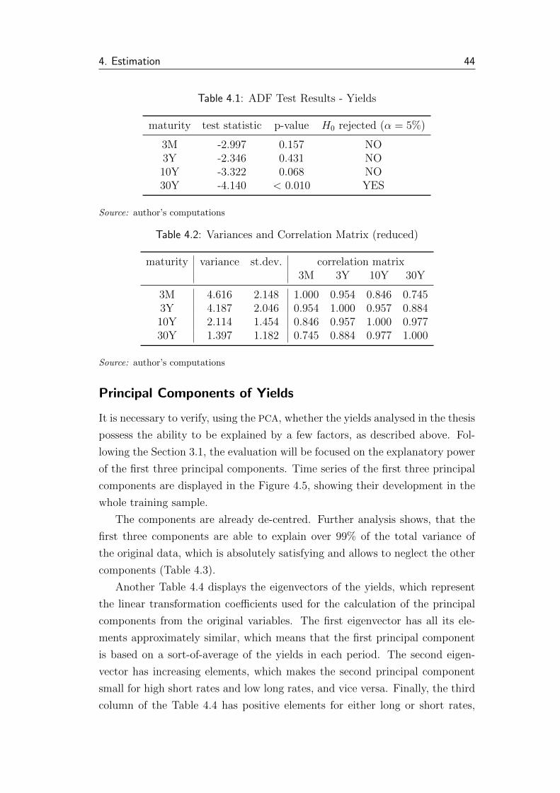
4. Estimation 44
Table 4.1: ADF Test Results - Yields
maturity test statistic p-value H0 rejected (α = 5%)
3M -2.997 0.157 NO3Y -2.346 0.431 NO10Y -3.322 0.068 NO30Y -4.140 < 0.010 YES
Source: author’s computations
Table 4.2: Variances and Correlation Matrix (reduced)
maturity variance st.dev. correlation matrix3M 3Y 10Y 30Y
3M 4.616 2.148 1.000 0.954 0.846 0.7453Y 4.187 2.046 0.954 1.000 0.957 0.88410Y 2.114 1.454 0.846 0.957 1.000 0.97730Y 1.397 1.182 0.745 0.884 0.977 1.000
Source: author’s computations
Principal Components of Yields
It is necessary to verify, using the PCA, whether the yields analysed in the thesis
possess the ability to be explained by a few factors, as described above. Fol-
lowing the Section 3.1, the evaluation will be focused on the explanatory power
of the first three principal components. Time series of the first three principal
components are displayed in the Figure 4.5, showing their development in the
whole training sample.
The components are already de-centred. Further analysis shows, that the
first three components are able to explain over 99% of the total variance of
the original data, which is absolutely satisfying and allows to neglect the other
components (Table 4.3).
Another Table 4.4 displays the eigenvectors of the yields, which represent
the linear transformation coefficients used for the calculation of the principal
components from the original variables. The first eigenvector has all its ele-
ments approximately similar, which means that the first principal component
is based on a sort-of-average of the yields in each period. The second eigen-
vector has increasing elements, which makes the second principal component
small for high short rates and low long rates, and vice versa. Finally, the third
column of the Table 4.4 has positive elements for either long or short rates,
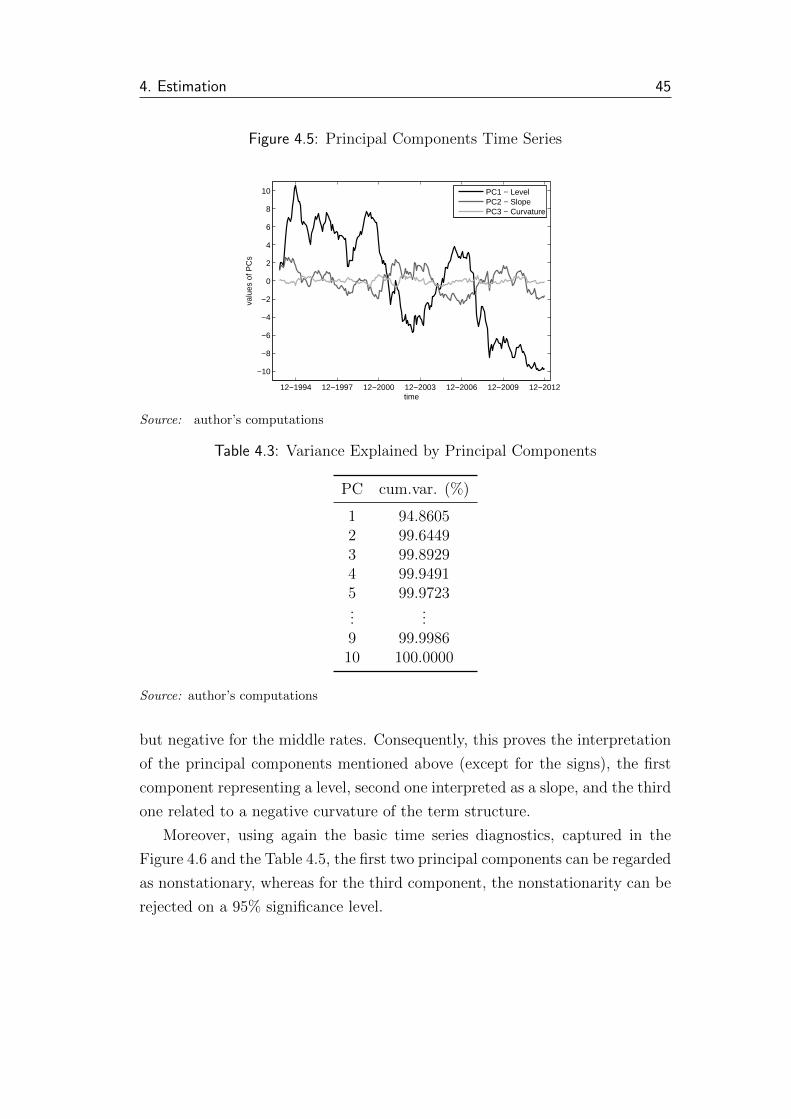
4. Estimation 45
Figure 4.5: Principal Components Time Series
12−1994 12−1997 12−2000 12−2003 12−2006 12−2009 12−2012
−10
−8
−6
−4
−2
0
2
4
6
8
10
time
valu
es o
f PC
s
PC1 − LevelPC2 − SlopePC3 − Curvature
Source: author’s computations
Table 4.3: Variance Explained by Principal Components
PC cum.var. (%)
1 94.86052 99.64493 99.89294 99.94915 99.9723...
...9 99.998610 100.0000
Source: author’s computations
but negative for the middle rates. Consequently, this proves the interpretation
of the principal components mentioned above (except for the signs), the first
component representing a level, second one interpreted as a slope, and the third
one related to a negative curvature of the term structure.
Moreover, using again the basic time series diagnostics, captured in the
Figure 4.6 and the Table 4.5, the first two principal components can be regarded
as nonstationary, whereas for the third component, the nonstationarity can be
rejected on a 95% significance level.
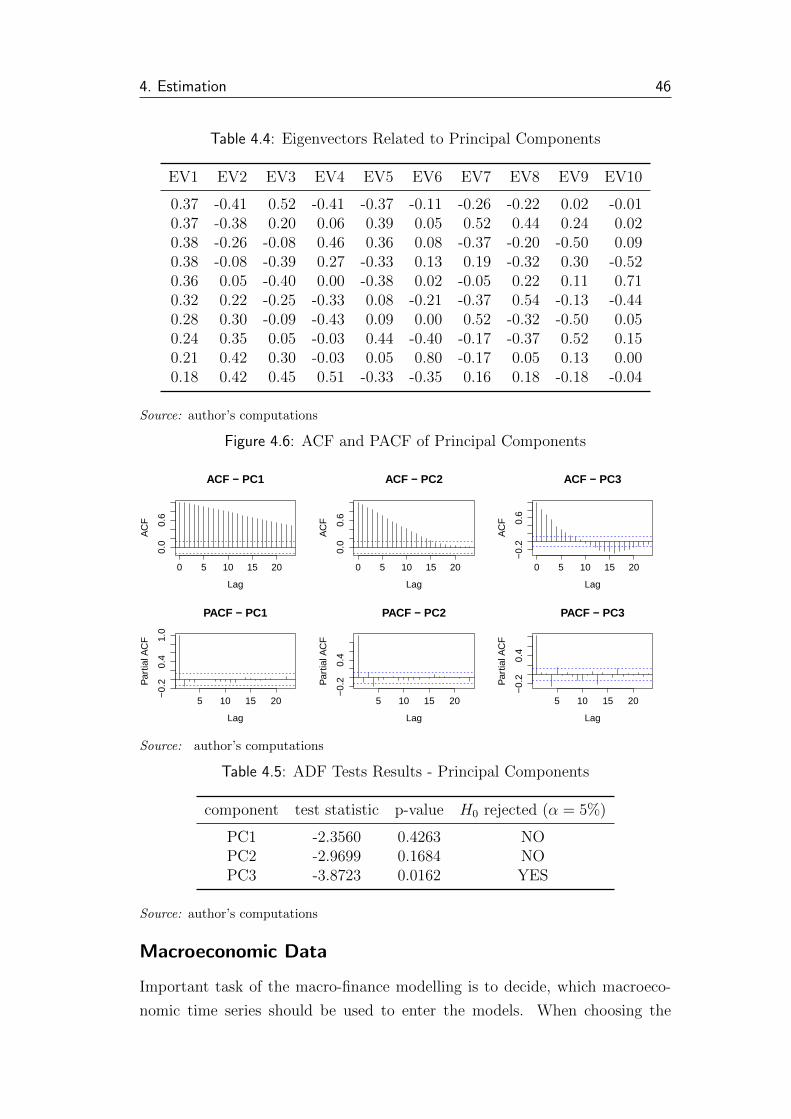
4. Estimation 46
Table 4.4: Eigenvectors Related to Principal Components
EV1 EV2 EV3 EV4 EV5 EV6 EV7 EV8 EV9 EV10
0.37 -0.41 0.52 -0.41 -0.37 -0.11 -0.26 -0.22 0.02 -0.010.37 -0.38 0.20 0.06 0.39 0.05 0.52 0.44 0.24 0.020.38 -0.26 -0.08 0.46 0.36 0.08 -0.37 -0.20 -0.50 0.090.38 -0.08 -0.39 0.27 -0.33 0.13 0.19 -0.32 0.30 -0.520.36 0.05 -0.40 0.00 -0.38 0.02 -0.05 0.22 0.11 0.710.32 0.22 -0.25 -0.33 0.08 -0.21 -0.37 0.54 -0.13 -0.440.28 0.30 -0.09 -0.43 0.09 0.00 0.52 -0.32 -0.50 0.050.24 0.35 0.05 -0.03 0.44 -0.40 -0.17 -0.37 0.52 0.150.21 0.42 0.30 -0.03 0.05 0.80 -0.17 0.05 0.13 0.000.18 0.42 0.45 0.51 -0.33 -0.35 0.16 0.18 -0.18 -0.04
Source: author’s computations
Figure 4.6: ACF and PACF of Principal Components
0 5 10 15 20
0.0
0.6
Lag
AC
F
ACF − PC1
5 10 15 20
−0.
20.
41.
0
Lag
Par
tial A
CF
PACF − PC1
0 5 10 15 20
0.0
0.6
Lag
AC
F
ACF − PC2
5 10 15 20
−0.
20.
4
Lag
Par
tial A
CF
PACF − PC2
0 5 10 15 20
−0.
20.
6
Lag
AC
F
ACF − PC3
5 10 15 20
−0.
20.
4
Lag
Par
tial A
CF
PACF − PC3
Source: author’s computations
Table 4.5: ADF Tests Results - Principal Components
component test statistic p-value H0 rejected (α = 5%)
PC1 -2.3560 0.4263 NOPC2 -2.9699 0.1684 NOPC3 -3.8723 0.0162 YES
Source: author’s computations
Macroeconomic Data
Important task of the macro-finance modelling is to decide, which macroeco-
nomic time series should be used to enter the models. When choosing the

4. Estimation 47
appropriate data, it is important to stick to the following points ensuring the
resulting models will be well-designed:
� It is necessary to synchronize the frequency of macroeconomic and finan-
cial data. For the thesis, it means to use the monthly periodicity, which
excludes the use of many series (particularly gross domestic product data,
which are released on a quarterly basis).
� Many authors (for example Choudhry 2011 or Diebold & Li 2006) men-
tion the relation of the yield curve behavior to the certain macroeco-
nomic dynamics. Authors either link the yields to several key variables
(Diebold & Li 2006, Kollar 2011), or to the factors extracted from a large
set of macroeconomic variables (commonly using the PCA) - for example
De Pooter et al. (2007), Monch (2006) or Ang & Piazzesi (2003). Regard-
less to the approach, the finally chosen variables often address following
aspects of the economy:
– business cycle position (production gap, level of unemployment etc.)
– domestic prices dynamics (expected and historical inflation in terms
of Consumers Price Index (CPI) or Producers Price Index, central
bank inflation target)
– monetary aggregates (money stock, reserves)
– foreign sector (exchange rates, foreign production, foreign interest
rates)
� Another caveat of including the macro variables is the fact that they
are usually released with a time delay, which has to be considered when
evaluating the predictive performance.
� As notes De Pooter et al. (2007), it is useful to work with the variables
in terms of their annual growth rates; the monthly growth rates tend to
be largely volatile, which might reduce their explanatory power.
Reflecting these facts, following variables will be used as representatives of
the key channels, through which the macro-economy impacts the term structure
of interest rates3:
3Inspired mostly by De Pooter et al. (2007) and Kollar (2011).

4. Estimation 48
Industrial Production Index (IPI) can be assumed to include the dynamics of the
business cycle situation of the economy. It moves in a similar way as the
growth of the gross domestic product, and, moreover, is calculated with
a monthly periodicity.
Consumer Price Index (CPI) is used as the most common measure of price changes.
Monetary Aggregate M1 (M1) can be believed to reflect both an intensity of the
monetary policy supportive/restrictive behavior and a response of the
financial institutions to it.4
U.S. Dollar Index (USDI), for the purposes of the thesis calculated as a trade-
weighted average of the exchange rates of the U.S.Dollar to the other
main global currencies, will be expected to represent the real effective
exchange rate of the currency.
In all cases, the annual growth rates are used. Sometimes, gap values (de-
viances from a long-term equilibria) are used in this causes, which is, however,
not suitable for purposes of the forecasting, due to a difficult determination of
the equilibrium value for the most recent variables - typically when the Hodrick-
Prescott filter is used to determine the equilibrium. Moreover, in case of M1,
the log-differences are used instead. Also, following the mentioned delay in the
data release, all macro-variables will be used in a one-period lag5. The time
series of the chosen variables captures theFigure 4.7.
When evaluating the time series properties, namely a stationarity of the
macro variables, the non-stationarity can be (on 95% significance level) re-
jected for all of them, using both the ACF functions for a graphical intuition
(Figure 4.8) and the ADF test for an exact evaluation (Table 4.6).
4A typical example of relevance of this variable is the situation in the Czech Republicat the end of the year 2013, when a side-product of the central bank interventions was aninflow of the additional money on the inter-bank market, which caused a downside shift ofthe Czech government bond yield curve.
5However, in the further text, in order to avoid a misleading indexing in the models, theone-period-lagged macroeconomic variables will be indexed as contemporary (i.e. Xt). Thiscan be supported by an argument, that instead of changing of the indexes, the interpretationis modified: variable Xt will be assumed to represent the value of the variable X released inthe time t.
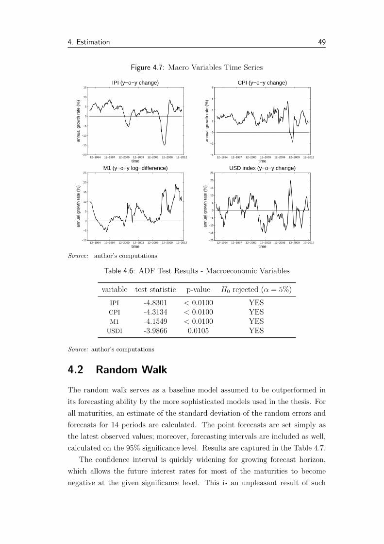
4. Estimation 49
Figure 4.7: Macro Variables Time Series
12−1994 12−1997 12−2000 12−2003 12−2006 12−2009 12−2012−20
−15
−10
−5
0
5
10
15
time
annu
al g
row
th r
ate
(%)
IPI (y−o−y change)
12−1994 12−1997 12−2000 12−2003 12−2006 12−2009 12−2012−4
−2
0
2
4
6
8
time
annu
al g
row
th r
ate
(%)
CPI (y−o−y change)
12−1994 12−1997 12−2000 12−2003 12−2006 12−2009 12−2012−10
−5
0
5
10
15
20
25
time
annu
al g
row
th r
ate
(%)
M1 (y−o−y log−difference)
12−1994 12−1997 12−2000 12−2003 12−2006 12−2009 12−2012−20
−15
−10
−5
0
5
10
15
20
25
time
annu
al g
row
th r
ate
(%)
USD index (y−o−y change)
Source: author’s computations
Table 4.6: ADF Test Results - Macroeconomic Variables
variable test statistic p-value H0 rejected (α = 5%)
IPI -4.8301 < 0.0100 YESCPI -4.3134 < 0.0100 YESM1 -4.1549 < 0.0100 YES
USDI -3.9866 0.0105 YES
Source: author’s computations
4.2 Random Walk
The random walk serves as a baseline model assumed to be outperformed in
its forecasting ability by the more sophisticated models used in the thesis. For
all maturities, an estimate of the standard deviation of the random errors and
forecasts for 14 periods are calculated. The point forecasts are set simply as
the latest observed values; moreover, forecasting intervals are included as well,
calculated on the 95% significance level. Results are captured in the Table 4.7.
The confidence interval is quickly widening for growing forecast horizon,
which allows the future interest rates for most of the maturities to become
negative at the given significance level. This is an unpleasant result of such
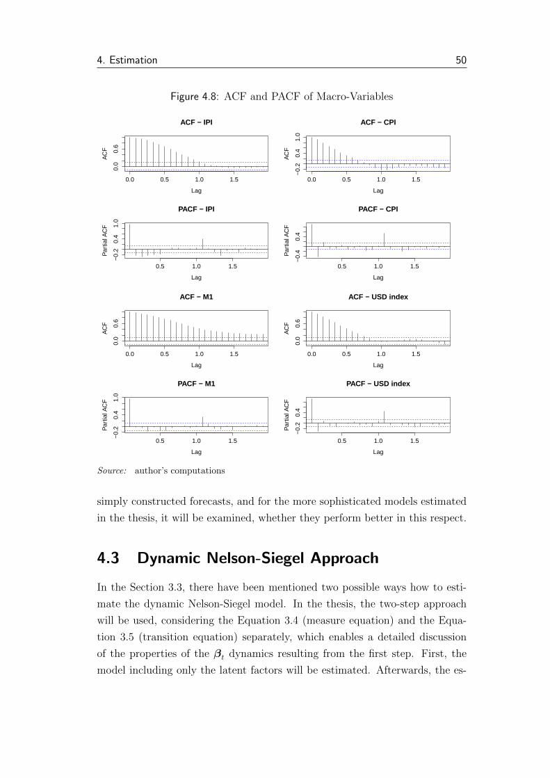
4. Estimation 50
Figure 4.8: ACF and PACF of Macro-Variables
0.0 0.5 1.0 1.5
0.0
0.6
Lag
AC
F
ACF − IPI
0.5 1.0 1.5
−0.
20.
41.
0
Lag
Par
tial A
CF
PACF − IPI
0.0 0.5 1.0 1.5
−0.
20.
41.
0
Lag
AC
F
ACF − CPI
0.5 1.0 1.5
−0.
40.
4
LagP
artia
l AC
F
PACF − CPI
0.0 0.5 1.0 1.5
0.0
0.6
Lag
AC
F
ACF − M1
0.5 1.0 1.5
−0.
20.
41.
0
Lag
Par
tial A
CF
PACF − M1
0.0 0.5 1.0 1.5
0.0
0.6
Lag
AC
F
ACF − USD index
0.5 1.0 1.5
−0.
20.
4
Lag
Par
tial A
CF
PACF − USD index
Source: author’s computations
simply constructed forecasts, and for the more sophisticated models estimated
in the thesis, it will be examined, whether they perform better in this respect.
4.3 Dynamic Nelson-Siegel Approach
In the Section 3.3, there have been mentioned two possible ways how to esti-
mate the dynamic Nelson-Siegel model. In the thesis, the two-step approach
will be used, considering the Equation 3.4 (measure equation) and the Equa-
tion 3.5 (transition equation) separately, which enables a detailed discussion
of the properties of the βt dynamics resulting from the first step. First, the
model including only the latent factors will be estimated. Afterwards, the es-

4. Estimation 51
Table 4.7: Random Walk Estimation & Forecasts
mat SD(a) PF1 LB1 UB1 PF6 LB6 UB6 PF14 LB14 UB14
3M 0.2303 0.05 -0.40 0.50 0.05 -1.06 1.16 0.05 -1.64 1.746M 0.2239 0.11 -0.33 0.55 0.11 -0.96 1.18 0.11 -1.53 1.751Y 0.2376 0.16 -0.31 0.63 0.16 -0.98 1.30 0.16 -1.58 1.902Y 0.2722 0.25 -0.28 0.78 0.25 -1.06 1.56 0.25 -1.75 2.253Y 0.2860 0.36 -0.20 0.92 0.36 -1.01 1.73 0.36 -1.74 2.465Y 0.2923 0.72 0.15 1.29 0.72 -0.68 2.12 0.72 -1.42 2.867Y 0.2869 1.18 0.62 1.74 1.18 -0.20 2.56 1.18 -0.92 3.28
10Y 0.2763 1.78 1.24 2.32 1.78 0.45 3.11 1.78 -0.25 3.8120Y 0.2511 2.54 2.05 3.03 2.54 1.33 3.75 2.54 0.70 4.3830Y 0.2415 2.95 2.47 3.42 2.95 1.79 4.11 2.95 1.18 4.72
mat = maturity; SD(a) = estimated standard deviation of the white noise;PF = point forecast; UB/LB = upper/lower bound on 95% confidence level;adjacent numbers represent prediction horizon in months
Source: author’s computations
timation will be replicated, extending the vector of the state factors by the
macroeconomic variables.
However, the very first task is to find the value of λ parameter, which plays
an important role in the Equation 3.4. Using the approach of Diebold & Li
(2006), maximizing the curvature for the maturity 30 months, the λA will result
directly from:
∂(
1−e−λAτλAτ
− e−λAτ)
∂τ
∣∣∣∣∣∣τ=2.5
= 0
After differentiating and plugging in for τ = 2.5, the λA is obtained from:
− 1
2.52λA+
2.5λAe−2.5λA + e−2.5λA
2.52λA+ λAe
−2.5λA = 0
Solving the equation numerically, the final result is:
λA.= 0.7173
Diebold & Li (2006) are using the maturity expressed in months instead, which
results in a significantly lower λA; however, after the value of λA is divided by
12, the results are similar.
The alternative approach is to obtain the optimal λ parameter value from
solving the expressions 3.8, 3.9 and 3.10. Some outputs of the minimization
problem6 are captured in the Table 4.8, the optimal λB has been found at the
6The minimization problem resulted in a single minima on the interval (0,170). For bigger

4. Estimation 52
value 0.5264.
Table 4.8: Nelson-Siegel RSS for Various λ Values
λB λA
λ: 0.001 0.1 0.5 0.5264 0.6 0.7173 1 10 100
RSS: 88.65 41.86 17.34 17.21 18.24 23.71 50.07 642.4 1070.1
Source: author’s computations
The preciseness of the fit is outlined by the Figure 4.9 for λA, respectively
by the Figure 4.11 for λB. Similarly, the development of the β parameters in
time is captured by the Figure 4.10 (and the Figure 4.12, respectively).
Figure 4.9: Fitted and Observed Values - Nelson-Siegel for λA
12−1994 12−1997 12−2000 12−2003 12−2006 12−2009 12−2012
0
1
2
3
4
5
6
7
8
time
yiel
d (%
)
3M fitted3M observed
12−1994 12−1997 12−2000 12−2003 12−2006 12−2009 12−2012
0
1
2
3
4
5
6
7
8
time
yiel
d (%
)
3Y fitted3Y observed
12−1994 12−1997 12−2000 12−2003 12−2006 12−2009 12−2012
0
1
2
3
4
5
6
7
8
time
yiel
d (%
)
10Y fitted10Y observed
12−1994 12−1997 12−2000 12−2003 12−2006 12−2009 12−2012
0
1
2
3
4
5
6
7
8
time
yiel
d (%
)
30Y fitted30Y observed
Source: author’s computations
As apparent from the figures, the level factor (β1) is almost equivalent in
both cases, whereas the other two factors slightly differ. Despite the fact they
have a similar interpretation, the βs resulting from the dynamic Nelson-Seigel
model differ from the principal components of the yields (Figure 4.5). The
values of λ, the matrix XTX is approaching singularity. It can be, however, intuitivelyassumed that the large values, related with an extremely fast exponential decay of the Nelson-Siegel function, cannot fit the values effectively, and the minimum can be hence consideredas the global minima for all positive λ. The optimal value has been obtained numerically inMATLAB.
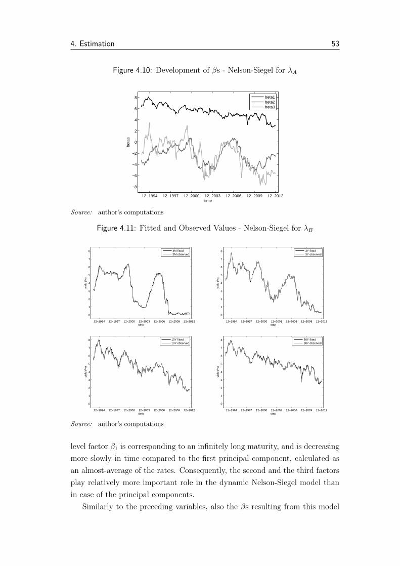
4. Estimation 53
Figure 4.10: Development of βs - Nelson-Siegel for λA
12−1994 12−1997 12−2000 12−2003 12−2006 12−2009 12−2012
−8
−6
−4
−2
0
2
4
6
8
time
beta
s
beta1beta2beta3
Source: author’s computations
Figure 4.11: Fitted and Observed Values - Nelson-Siegel for λB
12−1994 12−1997 12−2000 12−2003 12−2006 12−2009 12−2012
0
1
2
3
4
5
6
7
8
time
yiel
d (%
)
3M fitted3M observed
12−1994 12−1997 12−2000 12−2003 12−2006 12−2009 12−2012
0
1
2
3
4
5
6
7
8
time
yiel
d (%
)
3Y fitted3Y observed
12−1994 12−1997 12−2000 12−2003 12−2006 12−2009 12−2012
0
1
2
3
4
5
6
7
8
time
yiel
d (%
)
10Y fitted10Y observed
12−1994 12−1997 12−2000 12−2003 12−2006 12−2009 12−2012
0
1
2
3
4
5
6
7
8
time
yiel
d (%
)
30Y fitted30Y observed
Source: author’s computations
level factor β1 is corresponding to an infinitely long maturity, and is decreasing
more slowly in time compared to the first principal component, calculated as
an almost-average of the rates. Consequently, the second and the third factors
play relatively more important role in the dynamic Nelson-Siegel model than
in case of the principal components.
Similarly to the preceding variables, also the βs resulting from this model

4. Estimation 54
Figure 4.12: Development of βs - Nelson-Siegel for λB
12−1994 12−1997 12−2000 12−2003 12−2006 12−2009 12−2012
−8
−6
−4
−2
0
2
4
6
8
time
beta
s
beta1beta2beta3
Source: author’s computations
should be described in terms of the time series properties. The results of the
ADF tests are in the Table 4.9. For both λA and λB, β1 has been rejected
to be non-stationary, which was not possible for either β2 or β3 on the 95%
significance level.
Table 4.9: ADF Test Results - Latent Factors (βs)
variable test statistic p-value H0 rejected (α = 5%)
β1,A -3.7844 0.0206 YESβ2,A -2.8315 0.2266 NOβ3,A -2.6064 0.3212 NOβ1,B -3.6519 0.0292 YESβ2,B -2.7954 0.2417 NOβ3,B -3.1884 0.0907 NO
Source: author’s computations
Latent-Factors-Only Models
After the βs are extracted, the estimation of the model itself can be done. Be-
fore it, it is important to note, that the VAR model is used despite the fact,
that some of the variables (namely β2 and β3) were not rejected to be non-
stationary. However, Sims et al. (1990) has shown, that the use of the VAR
model for the datasets containing both stationary and non-stationary variables
is still possible without a loss of the model consistency or performing a spu-
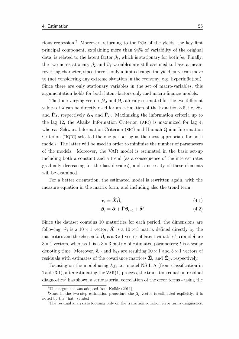
4. Estimation 55
rious regression.7 Moreover, returning to the PCA of the yields, the key first
principal component, explaining more than 94% of variability of the original
data, is related to the latent factor β1, which is stationary for both λs. Finally,
the two non-stationary β2 and β3 variables are still assumed to have a mean-
reverting character, since there is only a limited range the yield curve can move
to (not considering any extreme situation in the economy, e.g. hyperinflation).
Since there are only stationary variables in the set of macro-variables, this
argumentation holds for both latent-factors-only and macro-finance models.
The time-varying vectors βA and βB already estimated for the two different
values of λ can be directly used for an estimation of the Equation 3.5, i.e. αA
and ΓA, respectively αB and ΓB. Maximizing the information criteria up to
the lag 12, the Akaike Information Criterion (AIC) is maximized for lag 4,
whereas Schwarz Information Criterion (SIC) and Hannah-Quinn Intormation
Criterion (HQIC) selected the one period lag as the most appropriate for both
models. The latter will be used in order to minimize the number of parameters
of the models. Moreover, the VAR model is estimated in the basic set-up
including both a constant and a trend (as a consequence of the interest rates
gradually decreasing for the last decades), and a necessity of these elements
will be examined.
For a better orientation, the estimated model is rewritten again, with the
measure equation in the matrix form, and including also the trend term:
rt = Xβt (4.1)
βt = α+ Γβt−1 + δt (4.2)
Since the dataset contains 10 maturities for each period, the dimensions are
following: rt is a 10 × 1 vector; X is a 10 × 3 matrix defined directly by the
maturities and the chosen λ; βt is a 3×1 vector of latent variables8; α and δ are
3× 1 vectors, whereas Γ is a 3× 3 matrix of estimated parameters; t is a scalar
denoting time. Moreover, εr,t and εβ,t are resulting 10× 1 and 3× 1 vectors of
residuals with estimates of the covariance matrices Σr and Σβ, respectively.
Focusing on the model using λA, i.e. model NS-L-A (from classification in
Table 3.1), after estimating the VAR(1) process, the transition equation residual
diagnostics9 has shown a serious serial correlation of the error terms - using the
7This argument was adopted from Kollar (2011).8Since in the two-step estimation procedure the βt vector is estimated explicitly, it is
noted by the ”hat” symbol9The residual analysis is focusing only on the transition equation error terms diagnostics,

4. Estimation 56
Breusch-Godfrey LM-statistic, the null hypothesis of absence of the serial cor-
relation was rejected on a significance level higher than 99,9%. This indicates a
wrong specification of the model, which might be resolved by adding more lags
to the models. In this case, the four-lagged version VAR(4) (as offered by the
AIC) is sufficient to resolve the problem (unable to reject the null hypothesis of
absence of the serial correlation of the Breusch-Godfrey test even on the 90%
significance level), changing the βt process estimation into the form:
βt = α+ Γ1βt−1 + Γ2βt−2 + Γ3βt−3 + Γ4βt−4 + δt (4.3)
The estimated model still indicates problems with a normality (which may be
considered as typical for the financial data models), and a related rejection of
the null hypothesis of homoscedasticity (using Engle’s ARCH test). On the
other hand, the VAR model can be considered as stable, with no roots of the
characteristic polynomial lying outside the unit circle. Since the mentioned
problems can be expected to be present for all estimated models, the model
will be, for purposes of a relative comparison of the predictive performance,
used in this form.
The estimated parameters (i.e. vectors and matrices of parameters) are
included in the Appendix A, as well as the Figure A.1 capturing the actual and
fitted values resulting from the VAR model, a plot of residuals and their ACF
and PACF.
The second model NS-L-B, equivalent to the previous except for the λB used
in this case, results in very similar estimation properties as the first model. The
VAR(4) model is again used due to the serial autocorrelation in the error term of
the VAR(1) model; the non-normality and a slight heretoscedasticity are present
as well, but the model is still stable in terms of the unit roots. The estimated
parameters are in the Appendix A, with the actual and fitted values, residuals
dynamics and their ACF and PACF captured in the Figure A.2.
Using the estimated models, values for future 14 periods may be calculated.
This forecasting will proceed analogically to the two steps of estimations (but
in the opposite direction):
� First, the βt+h,A, for h = {1, 2...14} will be calculated by iterative plug-
since the measure equation error term has in the case of the two-step estimation rather atechnical character, and was sufficiently described in the section dealing with the estimationof λ parameter.

4. Estimation 57
ging into the Equation 4.3 with the parameters estimated for the NS-L-A
model.
� Then, pre-multiplying the βt+h,A vector by the XA matrix, the forecasts
of rt+h are obtained.
� The process is replicated also using the estimation of the transition equa-
tion NS-L-B, βt+h,B and XB.
Some of the estimations are displayed in the tables 4.10 and 4.11.
Table 4.10: NS-L-A Forecasts
PF1 LB1 UB1 PF6 LB6 UB6 PF14 LB14 UB14
β1,A 3.19 2.71 3.66 3.44 2.51 4.37 3.39 2.42 4.37β2,A -2.74 -3.4 -2.09 -2.99 -4.6 -1.39 -3.06 -5.48 -0.64β3,A -5.47 -6.91 -4.04 -5.1 -8.06 -2.14 -5.64 -8.98 -2.3
3M 0.24 -0.95 1.43 0.3 -2.34 2.93 0.15 -3.31 3.66M 0.11 -1.12 1.33 0.21 -2.49 2.9 0.03 -3.45 3.511Y -0.01 -1.27 1.26 0.16 -2.59 2.9 -0.06 -3.51 3.392Y 0.13 -1.11 1.37 0.36 -2.29 3.01 0.12 -3.12 3.363Y 0.45 -0.72 1.61 0.71 -1.75 3.17 0.48 -2.47 3.435Y 1.11 0.11 2.11 1.39 -0.69 3.47 1.19 -1.25 3.647Y 1.6 0.72 2.47 1.88 0.06 3.69 1.71 -0.38 3.8
10Y 2.05 1.28 2.81 2.32 0.76 3.88 2.19 0.41 3.9620Y 2.61 1.99 3.23 2.88 1.63 4.13 2.79 1.41 4.1730Y 2.8 2.23 3.37 3.07 1.93 4.21 2.99 1.75 4.23
notes: see Table 4.7
Source: author’s computations
Since the model is largely over-parametrized, a discussion of the values of
elements of the α and δ vectors and Γ matrices is not very useful. However,
it may be interesting to examine the impulse-response functions resulting from
the models — Figure 4.13. The implications resulting from the estimations and
the IRF, as well as the accuracy of the forecasts, will be into a detail described
in the Chapter 5 in the context of other models’ estimation and performance.
Macro-Finance Models
The macro-finance models, based on the dynamic Nelson-Siegel approach, will
utilize the already estimated λA and λB parameters, as well as βt,A, respectively
βt,B time-varying vectors. Different will be the transition equation, described
by the Equation 3.7, with the ηt including seven elements - three β latent

4. Estimation 58
Table 4.11: NS-L-B Forecasts
PF1 LB1 UB1 PF6 LB6 UB6 PF14 LB14 UB14
β1,B 3.44 2.98 3.9 3.66 2.77 4.55 3.63 2.68 4.58β2,B -3.18 -3.82 -2.55 -3.43 -5.1 -1.76 -3.56 -6.09 -1.04β3,B -4.71 -6.15 -3.27 -4.19 -6.96 -1.42 -4.64 -7.58 -1.7
3M 0.17 -0.97 1.31 0.19 -2.43 2.82 0.01 -3.48 3.56M 0.12 -1.06 1.29 0.18 -2.49 2.85 -0.02 -3.51 3.471Y 0.08 -1.14 1.3 0.21 -2.5 2.92 -0.01 -3.47 3.452Y 0.2 -1.04 1.44 0.41 -2.26 3.08 0.18 -3.12 3.473Y 0.44 -0.77 1.64 0.69 -1.86 3.25 0.46 -2.63 3.555Y 0.99 -0.1 2.08 1.28 -0.98 3.53 1.07 -1.59 3.737Y 1.47 0.49 2.44 1.75 -0.25 3.75 1.58 -0.74 3.89
10Y 1.97 1.12 2.81 2.24 0.53 3.96 2.1 0.14 4.0720Y 2.69 2.03 3.34 2.94 1.62 4.25 2.85 1.39 4.3230Y 2.94 2.34 3.53 3.18 2.01 4.35 3.11 1.82 4.4
notes: see Table 4.7
Source: author’s computations
Figure 4.13: IRF of NS-L-A and NS-L-B
xy$x
beta
1A
−0.
20.
00.
2
xy$x
beta
2A
−0.
20.
00.
2
xy$x
beta
3A
−0.
20.
00.
2
0 1 2 3 4 5 6 7 8 9 10
Orthogonal Impulse Response from beta1A
95 % Bootstrap CI, 100 runs
xy$x
beta
1A
−0.
20.
00.
2
xy$x
beta
2A
−0.
20.
00.
2
xy$x
beta
3A
−0.
20.
00.
2
0 1 2 3 4 5 6 7 8 9 10
Orthogonal Impulse Response from beta2A
95 % Bootstrap CI, 100 runs
xy$x
beta
1A
0.0
0.4
0.8
xy$x
beta
2A
0.0
0.4
0.8
xy$x
beta
3A
0.0
0.4
0.8
0 1 2 3 4 5 6 7 8 9 10
Orthogonal Impulse Response from beta3A
95 % Bootstrap CI, 100 runs
xy$x
beta
1B
−0.
20.
00.
2
xy$x
beta
2B
−0.
20.
00.
2
xy$x
beta
3B
−0.
20.
00.
2
0 1 2 3 4 5 6 7 8 9 10
Orthogonal Impulse Response from beta1B
95 % Bootstrap CI, 100 runs
xy$x
beta
1B
−0.
10.
10.
3
xy$x
beta
2B
−0.
10.
10.
3
xy$x
beta
3B
−0.
10.
10.
3
0 1 2 3 4 5 6 7 8 9 10
Orthogonal Impulse Response from beta2B
95 % Bootstrap CI, 100 runs
xy$x
beta
1B
0.0
0.4
xy$x
beta
2B
0.0
0.4
xy$x
beta
3B
0.0
0.4
0 1 2 3 4 5 6 7 8 9 10
Orthogonal Impulse Response from beta3B
95 % Bootstrap CI, 100 runs
Source: author’s computations
factors and four macroeconomic variables mentioned above: IPI, CPI, M1 and
USDI.
In the case of the macro-finance models NS-M-A and NS-M-B (which dif-
fer in the λ values as determined above), it comes out that the inclusion of
deterministic trend is unnecessary, or even biasing the model, leading to high
serial correlation of residuals. This may be considered as a signal, that the
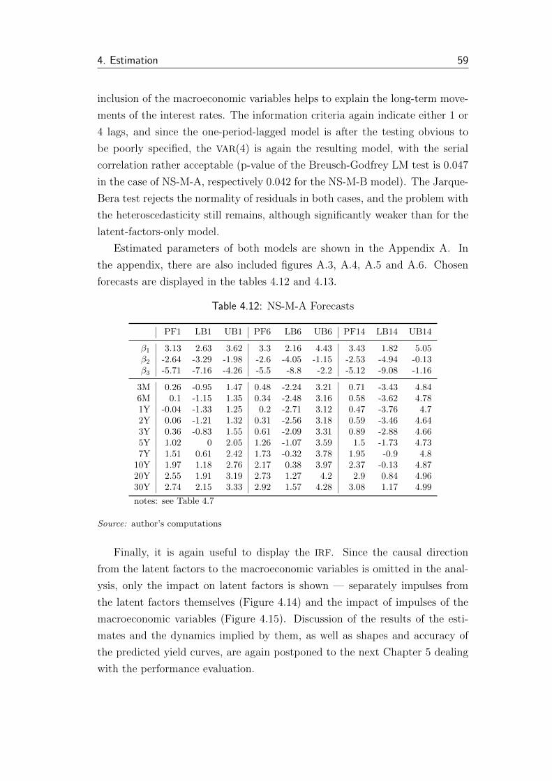
4. Estimation 59
inclusion of the macroeconomic variables helps to explain the long-term move-
ments of the interest rates. The information criteria again indicate either 1 or
4 lags, and since the one-period-lagged model is after the testing obvious to
be poorly specified, the VAR(4) is again the resulting model, with the serial
correlation rather acceptable (p-value of the Breusch-Godfrey LM test is 0.047
in the case of NS-M-A, respectively 0.042 for the NS-M-B model). The Jarque-
Bera test rejects the normality of residuals in both cases, and the problem with
the heteroscedasticity still remains, although significantly weaker than for the
latent-factors-only model.
Estimated parameters of both models are shown in the Appendix A. In
the appendix, there are also included figures A.3, A.4, A.5 and A.6. Chosen
forecasts are displayed in the tables 4.12 and 4.13.
Table 4.12: NS-M-A Forecasts
PF1 LB1 UB1 PF6 LB6 UB6 PF14 LB14 UB14
β1 3.13 2.63 3.62 3.3 2.16 4.43 3.43 1.82 5.05β2 -2.64 -3.29 -1.98 -2.6 -4.05 -1.15 -2.53 -4.94 -0.13β3 -5.71 -7.16 -4.26 -5.5 -8.8 -2.2 -5.12 -9.08 -1.16
3M 0.26 -0.95 1.47 0.48 -2.24 3.21 0.71 -3.43 4.846M 0.1 -1.15 1.35 0.34 -2.48 3.16 0.58 -3.62 4.781Y -0.04 -1.33 1.25 0.2 -2.71 3.12 0.47 -3.76 4.72Y 0.06 -1.21 1.32 0.31 -2.56 3.18 0.59 -3.46 4.643Y 0.36 -0.83 1.55 0.61 -2.09 3.31 0.89 -2.88 4.665Y 1.02 0 2.05 1.26 -1.07 3.59 1.5 -1.73 4.737Y 1.51 0.61 2.42 1.73 -0.32 3.78 1.95 -0.9 4.8
10Y 1.97 1.18 2.76 2.17 0.38 3.97 2.37 -0.13 4.8720Y 2.55 1.91 3.19 2.73 1.27 4.2 2.9 0.84 4.9630Y 2.74 2.15 3.33 2.92 1.57 4.28 3.08 1.17 4.99
notes: see Table 4.7
Source: author’s computations
Finally, it is again useful to display the IRF. Since the causal direction
from the latent factors to the macroeconomic variables is omitted in the anal-
ysis, only the impact on latent factors is shown — separately impulses from
the latent factors themselves (Figure 4.14) and the impact of impulses of the
macroeconomic variables (Figure 4.15). Discussion of the results of the esti-
mates and the dynamics implied by them, as well as shapes and accuracy of
the predicted yield curves, are again postponed to the next Chapter 5 dealing
with the performance evaluation.

4. Estimation 60
Table 4.13: NS-M-B Forecasts
PF1 LB1 UB1 PF6 LB6 UB6 PF14 LB14 UB14
β1 3.4 2.92 3.88 3.56 2.49 4.63 3.67 2.14 5.2β2 -3.11 -3.74 -2.48 -3.09 -4.57 -1.6 -2.97 -5.47 -0.46β3 -4.97 -6.42 -3.51 -4.69 -7.84 -1.55 -4.34 -7.95 -0.73
3M 0.18 -0.97 1.34 0.38 -2.27 3.04 0.63 -3.47 4.736M 0.11 -1.08 1.31 0.33 -2.4 3.05 0.58 -3.55 4.721Y 0.05 -1.19 1.29 0.28 -2.53 3.1 0.55 -3.6 4.712Y 0.14 -1.13 1.4 0.39 -2.45 3.22 0.67 -3.39 4.723Y 0.36 -0.87 1.59 0.62 -2.13 3.37 0.89 -2.97 4.755Y 0.91 -0.2 2.02 1.15 -1.32 3.63 1.41 -2.02 4.847Y 1.39 0.39 2.38 1.62 -0.6 3.84 1.85 -1.21 4.91
10Y 1.9 1.03 2.76 2.11 0.18 4.04 2.31 -0.36 4.9820Y 2.63 1.95 3.31 2.82 1.31 4.33 2.98 0.87 5.0930Y 2.89 2.28 3.5 3.07 1.7 4.43 3.21 1.29 5.13
notes: see Table 4.7
Source: author’s computations
Figure 4.14: IRF of NS-M-A and NS-M-B: part 1
xy$x
beta
1A
−0.
20.
20.
4
xy$x
beta
2A
−0.
20.
20.
4
xy$x
beta
3A
−0.
20.
20.
4
0 1 2 3 4 5 6 7 8 9 10
Orthogonal Impulse Response from beta1A
95 % Bootstrap CI, 100 runs
xy$x
beta
1A
−0.
10.
1
xy$x
beta
2A
−0.
10.
1
xy$x
beta
3A
−0.
10.
1
0 1 2 3 4 5 6 7 8 9 10
Orthogonal Impulse Response from beta2A
95 % Bootstrap CI, 100 runs
xy$x
beta
1A
0.0
0.2
0.4
0.6
xy$x
beta
2A
0.0
0.2
0.4
0.6
xy$x
beta
3A
0.0
0.2
0.4
0.6
0 1 2 3 4 5 6 7 8 9 10
Orthogonal Impulse Response from beta3A
95 % Bootstrap CI, 100 runs
xy$x
beta
1B
−0.
20.
00.
20.
4
xy$x
beta
2B
−0.
20.
00.
20.
4
xy$x
beta
3B
−0.
20.
00.
20.
4
0 1 2 3 4 5 6 7 8 9 10
Orthogonal Impulse Response from beta1B
95 % Bootstrap CI, 100 runs
xy$x
beta
1B
−0.
10.
10.
2
xy$x
beta
2B
−0.
10.
10.
2
xy$x
beta
3B
−0.
10.
10.
2
0 1 2 3 4 5 6 7 8 9 10
Orthogonal Impulse Response from beta2B
95 % Bootstrap CI, 100 runs
xy$x
beta
1B
0.0
0.2
0.4
0.6
xy$x
beta
2B
0.0
0.2
0.4
0.6
xy$x
beta
3B
0.0
0.2
0.4
0.6
0 1 2 3 4 5 6 7 8 9 10
Orthogonal Impulse Response from beta3B
95 % Bootstrap CI, 100 runs
Source: author’s computations
4.4 Affine Models
The estimation of the two affine models — latent-factors-only (henceforth noted
AF-L) model and macro-finance (AF-M) model — will follow the steps intro-
duced in the Section 3.4. The first three principal components have been al-
ready obtained in the Section 4.1, and based on them and the macroeconomic
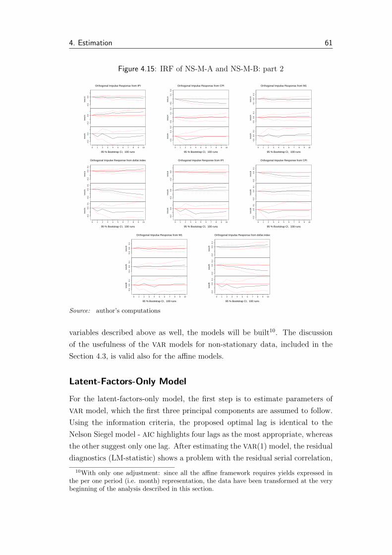
4. Estimation 61
Figure 4.15: IRF of NS-M-A and NS-M-B: part 2
xy$x
beta
1A
−0.
20.
0
xy$x
beta
2A
−0.
20.
0
xy$x
beta
3A
−0.
20.
0
0 1 2 3 4 5 6 7 8 9 10
Orthogonal Impulse Response from IPI
95 % Bootstrap CI, 100 runs
xy$x
beta
1A
−0.
10.
10.
2
xy$x
beta
2A
−0.
10.
10.
2
xy$x
beta
3A
−0.
10.
10.
2
0 1 2 3 4 5 6 7 8 9 10
Orthogonal Impulse Response from CPI
95 % Bootstrap CI, 100 runs
xy$x
beta
1A
−0.
10.
00.
1
xy$x
beta
2A
−0.
10.
00.
1
xy$x
beta
3A
−0.
10.
00.
1
0 1 2 3 4 5 6 7 8 9 10
Orthogonal Impulse Response from M1
95 % Bootstrap CI, 100 runs
xy$x
beta
1A
−0.
20.
00.
1
xy$x
beta
2A
−0.
20.
00.
1
xy$x
beta
3A
−0.
20.
00.
1
0 1 2 3 4 5 6 7 8 9 10
Orthogonal Impulse Response from dollar.index
95 % Bootstrap CI, 100 runs
xy$x
beta
1B
−0.
20.
0
xy$x
beta
2B
−0.
20.
0
xy$x
beta
3B
−0.
20.
0
0 1 2 3 4 5 6 7 8 9 10
Orthogonal Impulse Response from IPI
95 % Bootstrap CI, 100 runs
xy$x
beta
1B
−0.
20.
00.
1
xy$x
beta
2B
−0.
20.
00.
1
xy$x
beta
3B
−0.
20.
00.
1
0 1 2 3 4 5 6 7 8 9 10
Orthogonal Impulse Response from CPI
95 % Bootstrap CI, 100 runs
xy$x
beta
1B
−0.
10.
00.
1
xy$x
beta
2B
−0.
10.
00.
1
xy$x
beta
3B
−0.
10.
00.
1
0 1 2 3 4 5 6 7 8 9 10
Orthogonal Impulse Response from M1
95 % Bootstrap CI, 100 runs
xy$x
beta
1B
−0.
20.
00.
1
xy$x
beta
2B
−0.
20.
00.
1
xy$x
beta
3B
−0.
20.
00.
1
0 1 2 3 4 5 6 7 8 9 10
Orthogonal Impulse Response from dollar.index
95 % Bootstrap CI, 100 runs
Source: author’s computations
variables described above as well, the models will be built10. The discussion
of the usefulness of the VAR models for non-stationary data, included in the
Section 4.3, is valid also for the affine models.
Latent-Factors-Only Model
For the latent-factors-only model, the first step is to estimate parameters of
VAR model, which the first three principal components are assumed to follow.
Using the information criteria, the proposed optimal lag is identical to the
Nelson Siegel model - AIC highlights four lags as the most appropriate, whereas
the other suggest only one lag. After estimating the VAR(1) model, the residual
diagnostics (LM-statistic) shows a problem with the residual serial correlation,
10With only one adjustment: since all the affine framework requires yields expressed inthe per one period (i.e. month) representation, the data have been transformed at the verybeginning of the analysis described in this section.

4. Estimation 62
similarly to the previous model. The problem has been resolved by a use of the
VAR(4) process (with a constant and without a trend).11
Before proceeding further, it is necessary to convert the VAR(4) model to
its VAR(1) representation, in order to insert the estimated parameters directly
into the Equation 3.33 without any modification of the model. This is done by
rewriting the Equation 3.35, enriching the original symbols with tildes in order
to keep the further notation simple and consistent:
Lt = γ0 + Γ1Lt−1 + Γ2Lt−2 + Γ3Lt−3 + Γ4Lt−4 + ΣLεt
Lt−1 = 0 + ILt−1 + 0Lt−2 + 0Lt−3 + 0Lt−4 + 0
Lt−2 = 0 + 0Lt−1 + ILt−2 + 0Lt−3 + 0Lt−4 + 0
Lt−3 = 0 + 0Lt−1 + 0Lt−2 + ILt−3 + 0Lt−4 + 0
which can be converted into a matrix form:Lt
Lt−1
Lt−2
Lt−3
=
γ0
0
0
0
+
Γ1 Γ2 Γ3 Γ4
I 0 0 0
0 I 0 0
0 0 I 0
Lt−1
Lt−2
Lt−3
Lt−4
+
ΣL 0 0 0
0 0 0 0
0 0 0 0
0 0 0 0
εt
0
0
0
Lt = γ0 + Γ1Lt−1 + ΣLεt (4.4)
This transformation allows to keep the key equations of the affine model un-
changed. However, the vector of the latent factors included into the model has
changed, enriched by the three lags. Consequently, the vectors dimension l,
used throughout the Section 3.4, is modified into 4l — similarly for matrices.
Matrices γ0, Γ1 and ΣL, built from estimated parameters of the VAR pro-
cess, are listed in the Appendix A. There is included also the Figure A.7
capturing the development of the actual and fitted values, as well as the ACF
and the PACF of the residuals. The impulse-responses resulting from the VAR
model are shown by the Figure 4.16 - implications will be discussed in the
Chapter 5, when comparing all the models.
The next step is to estimate the dynamics of the short rate (Equation 3.12).
The vector of the latent factors includes also the lagged values resulting from
the VAR(4) adjustment. Since the shortest maturity included in the sample
is three months, this will be assumed to represent the short rate. Using OLS,
11Similarly to the Section 4.3, the general assumptions imposed on the error term arenot fulfilled in terms of the normality and the homoscedasticity; however, following similarstudies, the models are used despite to this fact, emphasising they are studied mainly fromtheir forecasting ability point of view, rather than examining the exact values of parameters.
4. Estimation 63
Figure 4.16: IRF of AF-L
xy$x
PC
1
0.00
0.04
0.08
xy$x
PC
2
0.00
0.04
0.08
xy$x
PC
3
0.00
0.04
0.08
0 1 2 3 4 5 6 7 8 9 10
Orthogonal Impulse Response from PC1
95 % Bootstrap CI, 100 runs
xy$x
PC
1
−0.
020.
01
xy$x
PC
2
−0.
020.
01
xy$x
PC
3
−0.
020.
01
0 1 2 3 4 5 6 7 8 9 10
Orthogonal Impulse Response from PC2
95 % Bootstrap CI, 100 runs
xy$x
PC
1
−0.
020.
000.
02
xy$x
PC
2
−0.
020.
000.
02
xy$x
PC
3
−0.
020.
000.
02
0 1 2 3 4 5 6 7 8 9 10
Orthogonal Impulse Response from PC3
95 % Bootstrap CI, 100 runs
Source: author’s computations
the estimates of the parameters a0 and a1 are obtained and included in the
Appendix A.
The last (and the most demanding) task is to find the optimal estimates of
λ0 and λ1 parameters values from the Equation 3.23. λ0 is in this case a 12-
dimensional vector, and λ1 is a 12×12-dimensional matrix of parameters, which
results in a high number (156) of parameters to be optimized jointly. However,
in the Equation 3.33 (which is crucial for the calculation of the optimal λ0
and λ1 values) the λ1 is pre-multiplied only by the ΣL matrix, which has zero
values for all rows or columns with the index higher than three: consequently,
without any impact on results, all rows of the λ1 matrix with the index higher
than three may be set to zero (similar argumentation holds for λ0 vector). This
reduces the number of the parameters to be estimates to only 39, which can be
considered as more eligible to enter the optimization procedure.
The procedure itself is built as follows: First, all the parameters are set to
their initial values equal to zero (following De Pooter et al. 2007). Then, since
the equation Equation 3.34 can be assumed to be differentiable with respect
to λ0 and λ1 (their elements), a gradient descent algorithm is used: in each
iteration, a partial derivative of the total difference between the observed and
model-implied yields (resulting from Equation 3.39) with respect to each of
the parameters to be optimized - relevant elements of λ0 and λ1 - is calculated
numerically, forming a gradient. Then, the new value of λ0 and λ1 is calculated
by subtracting the gradient from the previous values, multiplied by a speed
parameter, which is set as decreasing gradually to ensure both an acceptable
speed of the convergence and the best possible fit.12. Resulting λ0 and λ1 can
be found in Appendix A.
12The procedure was written manually in MATLAB. Final λ0 and λ1 were obtained atthe moment when a decrease of the RSS (Equation 3.40) between two iterations was smallerthan 10−6. This approach didn’t converge to the absolute minima of the function, and the
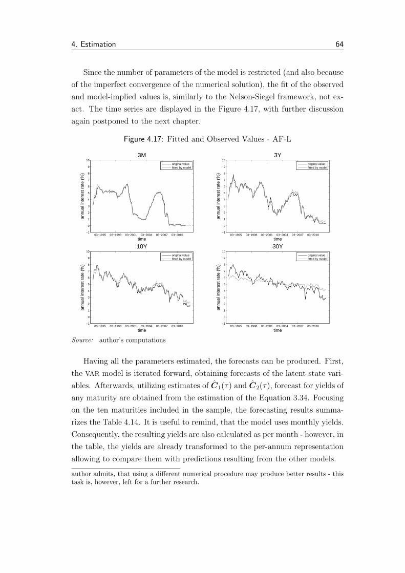
4. Estimation 64
Since the number of parameters of the model is restricted (and also because
of the imperfect convergence of the numerical solution), the fit of the observed
and model-implied values is, similarly to the Nelson-Siegel framework, not ex-
act. The time series are displayed in the Figure 4.17, with further discussion
again postponed to the next chapter.
Figure 4.17: Fitted and Observed Values - AF-L
03−1995 03−1998 03−2001 03−2004 03−2007 03−2010−1
0
1
2
3
4
5
6
7
8
9
10
time
annu
al in
tere
st r
ate
(%)
3M
original valuefitted by model
03−1995 03−1998 03−2001 03−2004 03−2007 03−2010−1
0
1
2
3
4
5
6
7
8
9
10
time
annu
al in
tere
st r
ate
(%)
3Y
original valuefitted by model
03−1995 03−1998 03−2001 03−2004 03−2007 03−2010−1
0
1
2
3
4
5
6
7
8
9
10
time
annu
al in
tere
st r
ate
(%)
10Y
original valuefitted by model
03−1995 03−1998 03−2001 03−2004 03−2007 03−2010−1
0
1
2
3
4
5
6
7
8
9
10
time
annu
al in
tere
st r
ate
(%)
30Y
original valuefitted by model
Source: author’s computations
Having all the parameters estimated, the forecasts can be produced. First,
the VAR model is iterated forward, obtaining forecasts of the latent state vari-
ables. Afterwards, utilizing estimates of C1(τ) and C2(τ), forecast for yields of
any maturity are obtained from the estimation of the Equation 3.34. Focusing
on the ten maturities included in the sample, the forecasting results summa-
rizes the Table 4.14. It is useful to remind, that the model uses monthly yields.
Consequently, the resulting yields are also calculated as per month - however, in
the table, the yields are already transformed to the per-annum representation
allowing to compare them with predictions resulting from the other models.
author admits, that using a different numerical procedure may produce better results - thistask is, however, left for a further research.

4. Estimation 65
Table 4.14: AF-L Forecasts
PF1 LB1 UB1 PF6 LB6 UB6 PF14 LB14 UB14
L1 -0.80 -0.91 -0.69 -0.79 -1.16 -0.43 -0.78 -1.36 -0.20L2 -0.12 -0.18 -0.06 -0.09 -0.24 0.05 -0.07 -0.26 0.12L3 -0.01 -0.04 0.02 -0.01 -0.06 0.03 -0.01 -0.06 0.04
3M 0.01 -0.33 0.35 -0.09 -1.27 1.09 -0.13 -2.04 1.796M -0.03 -0.41 0.36 -0.10 -1.30 1.09 -0.13 -2.06 1.811Y 0.05 -0.38 0.47 0.00 -1.22 1.21 -0.01 -1.98 1.962Y 0.39 -0.08 0.86 0.37 -0.92 1.66 0.38 -1.68 2.453Y 0.70 0.19 1.21 0.70 -0.67 2.07 0.73 -1.41 2.875Y 1.20 0.64 1.77 1.24 -0.23 2.71 1.30 -0.92 3.537Y 1.67 1.08 2.26 1.73 0.23 3.24 1.81 -0.42 4.05
10Y 2.35 1.76 2.94 2.43 0.95 3.91 2.53 0.38 4.6720Y 3.64 3.18 4.10 3.72 2.6 4.84 3.82 2.26 5.3730Y 4.20 3.88 4.52 4.26 3.49 5.04 4.33 3.27 5.40
notes: see Table 4.7
Source: author’s computations
Macro-Finance Model
Information criteria of the VAR model for the vector of state variables extended
by the macro-variables give the same results as in the previous case. However,
the model is not in this case specified well (it terms of the serial correlation
tests) for any reasonable lag, either with or without constant or even the time
trend. Following similar studies and keeping consistency thorough the thesis,
the model will be still estimated and commented on, utilizing the already men-
tioned flexibility of the VAR models. To reduce the number of parameters to
minimum, the VAR(1) model (again with a constant and without a time trend)
is henceforth estimated. Matrices ˆγ0,ˆΓ1 and ˆΣL, based on the estimated pa-
rameters of the VAR process, are included in the Appendix A, as well as the
Figure A.8 including the fitted values and the time series, ACF and PACF of
residuals. Moreover, Figure 4.18 includes the IRF of the model, with implica-
tions postponed to the next chapter.
The parameters of the short rate equation as well as ˆλ0 and ˆλ1 are obtained
in the very same way as in the case of the previous model. Fitted and observed
values are compared by the Figure 4.19. Moreover, the Table 4.15 includes a
sample of predictions, again for the 14-month horizon.
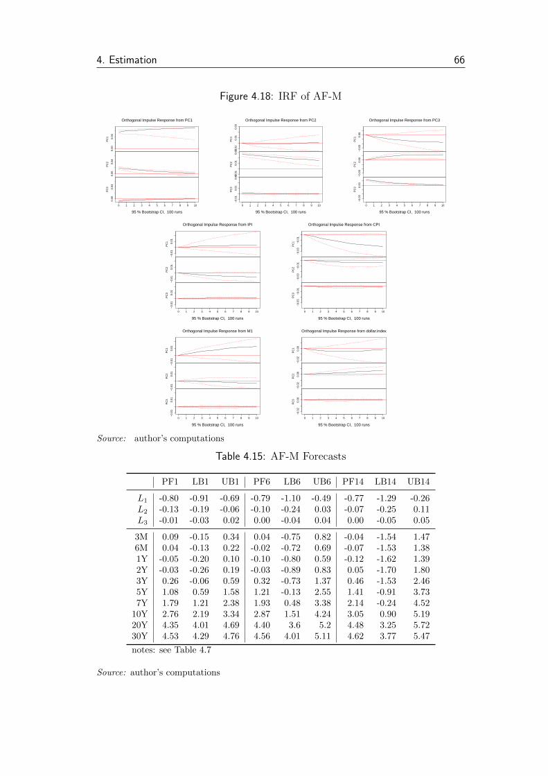
4. Estimation 66
Figure 4.18: IRF of AF-M
xy$x
PC
1
0.00
0.04
xy$x
PC
2
0.00
0.04
xy$x
PC
3
0.00
0.04
0 1 2 3 4 5 6 7 8 9 10
Orthogonal Impulse Response from PC1
95 % Bootstrap CI, 100 runs
xy$x
PC
1
−0.
010.
010.
03
xy$x
PC
2
−0.
010.
010.
03
xy$x
PC
3
−0.
010.
010.
03
0 1 2 3 4 5 6 7 8 9 10
Orthogonal Impulse Response from PC2
95 % Bootstrap CI, 100 runs
xy$x
PC
1
−0.
030.
00
xy$x
PC
2
−0.
030.
00
xy$x
PC
3
−0.
030.
00
0 1 2 3 4 5 6 7 8 9 10
Orthogonal Impulse Response from PC3
95 % Bootstrap CI, 100 runs
xy$x
PC
1
−0.
010.
01
xy$x
PC
2
−0.
010.
01
xy$x
PC
3
−0.
010.
01
0 1 2 3 4 5 6 7 8 9 10
Orthogonal Impulse Response from IPI
95 % Bootstrap CI, 100 runs
xy$x
PC
1
−0.
03−
0.01
xy$xP
C2
−0.
03−
0.01
xy$x
PC
3
−0.
03−
0.01
0 1 2 3 4 5 6 7 8 9 10
Orthogonal Impulse Response from CPI
95 % Bootstrap CI, 100 runs
xy$x
PC
1
−0.
010.
01
xy$x
PC
2
−0.
010.
01
xy$x
PC
3
−0.
010.
01
0 1 2 3 4 5 6 7 8 9 10
Orthogonal Impulse Response from M1
95 % Bootstrap CI, 100 runs
xy$x
PC
1
−0.
020.
00
xy$x
PC
2
−0.
020.
00
xy$x
PC
3
−0.
020.
00
0 1 2 3 4 5 6 7 8 9 10
Orthogonal Impulse Response from dollar.index
95 % Bootstrap CI, 100 runs
Source: author’s computations
Table 4.15: AF-M Forecasts
PF1 LB1 UB1 PF6 LB6 UB6 PF14 LB14 UB14
L1 -0.80 -0.91 -0.69 -0.79 -1.10 -0.49 -0.77 -1.29 -0.26L2 -0.13 -0.19 -0.06 -0.10 -0.24 0.03 -0.07 -0.25 0.11L3 -0.01 -0.03 0.02 0.00 -0.04 0.04 0.00 -0.05 0.05
3M 0.09 -0.15 0.34 0.04 -0.75 0.82 -0.04 -1.54 1.476M 0.04 -0.13 0.22 -0.02 -0.72 0.69 -0.07 -1.53 1.381Y -0.05 -0.20 0.10 -0.10 -0.80 0.59 -0.12 -1.62 1.392Y -0.03 -0.26 0.19 -0.03 -0.89 0.83 0.05 -1.70 1.803Y 0.26 -0.06 0.59 0.32 -0.73 1.37 0.46 -1.53 2.465Y 1.08 0.59 1.58 1.21 -0.13 2.55 1.41 -0.91 3.737Y 1.79 1.21 2.38 1.93 0.48 3.38 2.14 -0.24 4.52
10Y 2.76 2.19 3.34 2.87 1.51 4.24 3.05 0.90 5.1920Y 4.35 4.01 4.69 4.40 3.6 5.2 4.48 3.25 5.7230Y 4.53 4.29 4.76 4.56 4.01 5.11 4.62 3.77 5.47
notes: see Table 4.7
Source: author’s computations

4. Estimation 67
Figure 4.19: Fitted and Observed Values - AF-M
12−1994 12−1997 12−2000 12−2003 12−2006 12−2009 12−2012−1
0
1
2
3
4
5
6
7
8
9
10
time
annu
al in
tere
st r
ate
(%)
3M
original valuefitted by model
12−1994 12−1997 12−2000 12−2003 12−2006 12−2009 12−2012−1
0
1
2
3
4
5
6
7
8
9
10
time
annu
al in
tere
st r
ate
(%)
3Y
original valuefitted by model
12−1994 12−1997 12−2000 12−2003 12−2006 12−2009 12−2012−1
0
1
2
3
4
5
6
7
8
9
10
time
annu
al in
tere
st r
ate
(%)
10Y
original valuefitted by model
12−1994 12−1997 12−2000 12−2003 12−2006 12−2009 12−2012−1
0
1
2
3
4
5
6
7
8
9
10
time
annu
al in
tere
st r
ate
(%)
30Y
original valuefitted by model
Source: author’s computations
Chapter 5
Performance Evaluation
5.1 In-Sample Characteristics
The first feature of the models to be evaluated is their in-sample performance.
In the thesis, it is measured as an accuracy of the model in terms of the sum
of squared differences between the actual and fitted values — the RSS. For
the Nelson-Siegel based models, the in-sample fit is the same for both latent-
factors-only and macro-finance models, depending only on the chosen value of
λ - it is not influenced by the estimated VAR process parameters. Contrary,
the fitted yields resulting from the affine models can be obtained only after
estimating the process for the state variables, utilizing parameters of the VAR
model, and hence is different for both approaches. Results for the models
includes the Table 5.1, together with the graphical illustration as captured by
figures 4.9, 4.11, 4.17 and 4.19.
Results clearly show that the fit is distinctively better for the Nelson-Siegel
framework. The main reason has been already mentioned — the basic Nelson-
Siegel approach is static (it is rather a statistic approach than a model), with
the term structure fitted for each period separately. However, the resulting
latent factors then enter an unrestricted VAR process, which may result in poor
predictive results, as will be tested below. Contrary, the affine models are more
complex, starting with imposing restrictions on the dynamics of the variables
— then, the model is fitted within boundaries of these restrictions, which is
both less flexible and more computationally demanding.1 On the other hand,
it is possible that the cross-equation restrictions may result in a more precise
1As noted in the previous chapter, the author admits that the estimation of parametersλ0 and λ1 has not converged to the optimal point, which might be an additional reason forthe poor fit of the affine models.

5. Performance Evaluation 69
Table 5.1: In-Sample Fit Results
AF-L AF-M NS-A NS-B
3M 3.51 3.27 2.86 2.476M 6.57 5.17 0.78 0.681Y 7.97 7.74 2.79 1.742Y 8.44 11.01 1.95 1.523Y 12.44 20.40 0.33 0.455Y 17.71 43.77 2.29 1.007Y 16.14 54.48 2.41 1.29
10Y 15.34 79.15 2.56 1.9020Y 66.22 151.50 5.49 4.1830Y 108.69 163.27 2.07 1.80
note: RSS calculated from in-sample periods 4-231 (Jan 1994 - Dec 2012).
First three months were omitted because of the lags included in some models.
Source: author’s computations
estimation of the dynamics of the state variables, which would support the
predictive performance of the affine models.
Moreover, not surprisingly, the NS-B models fits the observed values better
than the NS-A model. This is resulting directly from the specification of the
λ parameter the models differ in - in case of NS-B, λ is estimated to ensure
an optimal fit, whereas in the other case, the λ is set in order to place the
”hump” into the most appropriate part of the yield curve. Focusing on the
affine models, the latent-factors-only model offers smaller RSS in case of longer
maturities (bigger than one year), whereas the short ones are fitted better by
the macro-finance model. In both affine cases, however, the fit is much worse
for the longest maturities than for the short ones.
To evaluate dynamic implications resulting from the estimated models, the
IRF of the VAR capturing development of the state variables will be used as a
both simple and representative tool. The responses are graphically captured by
the figures 4.13, 4.14 and 4.15 for the dynamic Nelson-Siegel models, and 4.16
and 4.18 for the affine approach. The most important findings are following:
NS-L-A and NS-L-B:
� An impulse from β1 might by related to structural changes in the be-
havior of economic subjects, changing either a required risk-premium
or a time preference of the subjects, often related to the expected
changes of the price level. This variable represents the level of the
5. Performance Evaluation 70
term structure — a yield for an infinite maturity in this case. As ob-
vious from the figures, the impact of the impulse is only temporary
- a positive shock into this variable is gradually fading, which might
be considered to be related to the business cycle dynamics. More-
over, as the positive shock represents the growth of the longest end
of the yield curve, it is accompanied by a growth of the slope (i.e. a
decrease of β2). The curvature first increases, but after six periods
(a half of a year), its dynamics change and it decreases instead.
� A positive shock from β2 - a decrease of a slope - may be represented
by a monetary policy step, typically in a period of a monetary pol-
icy restriction. Despite the fact that the short rate jumps up, IRF
implies that it has no effect on the long rate, which is in line with
the reality preceding the Lehman-Brothers crisis — the unsuccessful
attempts of FED to increase the longer rates in order to decelerate
the unhealthy economic boom.
NS-M-A and NS-M-B:
� Impulses from βs are in case of the macro-finance models very similar
to the previous, however the shocks are slightly more persistent.
� The impact of the macro-variables is also in line with the macroeco-
nomic reality. A positive shock in the production, growth of the price
level, increase of the money supply as well as a depreciation of the
U.S.Dollar are all related to the well-performing economy2. Follow-
ing such impulses, β1 — the level — is gradually slightly decreasing,
i.e. the longest rates are shifted down, which is traditionally related
to a decrease of the risk premium in the periods of conjuncture.
On the other hand, these parts of the economic cycle are related to
the already mentioned attempts of the central banks to restrict the
boom to a reasonable level, which results in a growth of the short
rate and hence a decrease of the slope of the term structure (and
growth of the β2 factor) - which is exactly what the IRF show.
AF-L:
� In the case of the affine models, the level variable, represented by
the first principal component, is calculated as a sort-of-average of all
2Either as a cause or an evidence
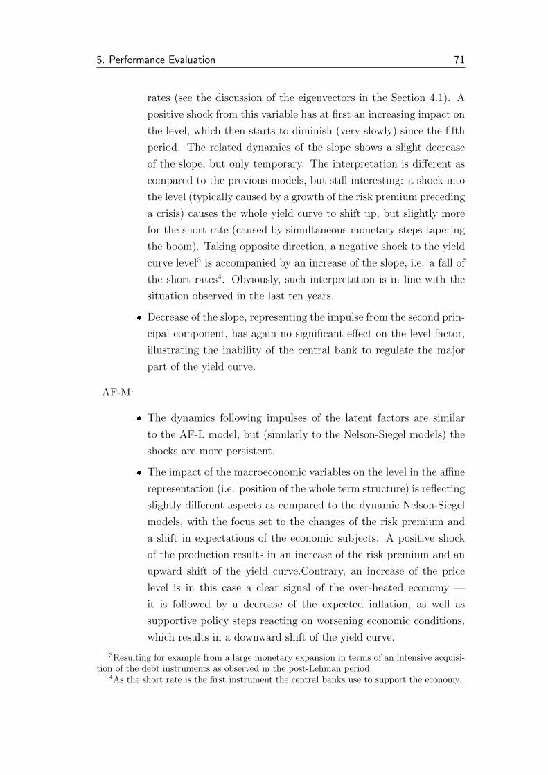
5. Performance Evaluation 71
rates (see the discussion of the eigenvectors in the Section 4.1). A
positive shock from this variable has at first an increasing impact on
the level, which then starts to diminish (very slowly) since the fifth
period. The related dynamics of the slope shows a slight decrease
of the slope, but only temporary. The interpretation is different as
compared to the previous models, but still interesting: a shock into
the level (typically caused by a growth of the risk premium preceding
a crisis) causes the whole yield curve to shift up, but slightly more
for the short rate (caused by simultaneous monetary steps tapering
the boom). Taking opposite direction, a negative shock to the yield
curve level3 is accompanied by an increase of the slope, i.e. a fall of
the short rates4. Obviously, such interpretation is in line with the
situation observed in the last ten years.
� Decrease of the slope, representing the impulse from the second prin-
cipal component, has again no significant effect on the level factor,
illustrating the inability of the central bank to regulate the major
part of the yield curve.
AF-M:
� The dynamics following impulses of the latent factors are similar
to the AF-L model, but (similarly to the Nelson-Siegel models) the
shocks are more persistent.
� The impact of the macroeconomic variables on the level in the affine
representation (i.e. position of the whole term structure) is reflecting
slightly different aspects as compared to the dynamic Nelson-Siegel
models, with the focus set to the changes of the risk premium and
a shift in expectations of the economic subjects. A positive shock
of the production results in an increase of the risk premium and an
upward shift of the yield curve.Contrary, an increase of the price
level is in this case a clear signal of the over-heated economy —
it is followed by a decrease of the expected inflation, as well as
supportive policy steps reacting on worsening economic conditions,
which results in a downward shift of the yield curve.
3Resulting for example from a large monetary expansion in terms of an intensive acquisi-tion of the debt instruments as observed in the post-Lehman period.
4As the short rate is the first instrument the central banks use to support the economy.
5. Performance Evaluation 72
� A more difficult task is to interpret the growth of the rates after
an increase of the money supply. This growth is gradual, and could
be related to changes of the expected inflation, which increases the
nominal rates. Finally, the impact of a currency depreciation on
the term structure is in the case of the AF-M model positive, which
might by related to the international capital flows.
A discussion of the dynamics of the third latent factor — curvature — is
intentionally omitted, since this variable is usually considered as both unim-
portant from the dynamic point of view and not easy to be given a intuitive
interpretation.
Obviously, the relations of the macroeconomic variables and interest rates
are based on many transition channels. However, intuitively, it can be signalled
by the interpretation of the IRF, that the dynamics implied by the affine mod-
els is more related to the financial markets situation (including the price of
risk, the monetary authority behavior on the markets, changes in expectations
etc.), whereas the Nelson-Siegel based models, not utilizing any restrictions
imposed on the rates and the market price of risk, are explaining rather the
general macroeconomic dynamics and a relation of the interest rates of various
maturities to the business cycle. This difference may be considered as implied
by the different definition of the level factor — in case of the affine models,
it represents a position of the whole yield curve, whereas the level within the
Nelson-Siegel approach is considered as an infinite maturity yield.
Most importantly, using the interpretation offered above, the dynamics ex-
plained by the macro-variables is offering an exact representation of the macro-
finance relations, i.e. impact of the macro-variables on different parts of the
yield curve, which is what was aimed to obtain by constructing the macro-
finance models.
5.2 Predictive Performance
The predictive performance will be first evaluated only for the single forecasting
period, with a detailed discussion of the results. However, such comparison is
not sufficient for an overall evaluation of the forecasting abilities of the models
— for this reason, all the models will be multiply re-estimated for shorter
periods rolling forward through the whole sample, which allows to conduct a
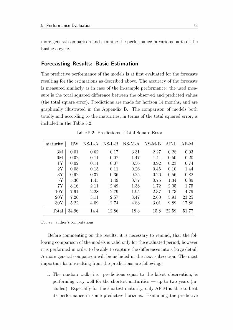
5. Performance Evaluation 73
more general comparison and examine the performance in various parts of the
business cycle.
Forecasting Results: Basic Estimation
The predictive performance of the models is at first evaluated for the forecasts
resulting for the estimations as described above. The accuracy of the forecasts
is measured similarly as in case of the in-sample performance: the used mea-
sure is the total squared difference between the observed and predicted values
(the total square error). Predictions are made for horizon 14 months, and are
graphically illustrated in the Appendix B. The comparison of models both
totally and according to the maturities, in terms of the total squared error, is
included in the Table 5.2.
Table 5.2: Predictions - Total Square Error
maturity RW NS-L-A NS-L-B NS-M-A NS-M-B AF-L AF-M
3M 0.01 0.62 0.17 3.31 2.27 0.28 0.036M 0.02 0.11 0.07 1.47 1.44 0.50 0.201Y 0.02 0.11 0.07 0.56 0.92 0.23 0.742Y 0.08 0.15 0.11 0.26 0.45 0.10 1.443Y 0.92 0.37 0.36 0.25 0.26 0.56 0.825Y 5.36 1.45 1.49 0.77 0.76 1.34 0.897Y 8.16 2.11 2.49 1.38 1.72 2.05 1.75
10Y 7.91 2.28 2.79 1.95 2.37 1.73 4.7920Y 7.26 3.11 2.57 3.47 2.60 5.91 23.2530Y 5.22 4.09 2.74 4.88 3.01 9.89 17.86
Total 34.96 14.4 12.86 18.3 15.8 22.59 51.77
Source: author’s computations
Before commenting on the results, it is necessary to remind, that the fol-
lowing comparison of the models is valid only for the evaluated period; however
it is performed in order to be able to capture the differences into a large detail.
A more general comparison will be included in the next subsection. The most
important facts resulting from the predictions are following:
1. The random walk, i.e. predictions equal to the latest observation, is
performing very well for the shortest maturities — up to two years (in-
cluded). Especially for the shortest maturity, only AF-M is able to beat
its performance in some predictive horizons. Examining the predictive

5. Performance Evaluation 74
quality into more detail, utilizing the Table 5.3 displaying the ranking of
the model for various combination of maturities and prediction horizons,
the model is the best predictor for either close horizon or short maturi-
ties. However, for longer maturities, almost all other models are able to
beat the naive predictions, especially for the horizon at least five months.
2. Focusing on the difference between the estimated models, similar tables
5.4 - 5.9 were created to offer a neat intuition about the performance.
Examining the difference between the Nelson-Siegel approach and affine
models, only for latent-factors-only models, the the NS-L-A and NS-L-B
models are better predictors for the short and medium horizon (across
all maturities5), whereas the AF-L model performs better for the longest
horizon. A reason for this lies in the fact, that the affine model implies
the term premium to be bigger than observed at the end of the in-sample
and the beginning of the out-of-sample period. However, since half of the
year 2013, the term premium is returning to the level expected by the
affine models.
3. Adding the macro-factors has a different impact on dynamic Nelson-Siegel
and affine models. In the first case, the macro-factors improve the per-
formance of the NS-L-A and NS-L-B models for the largest horizon, i.e.
extend the usefulness of these models — in some cases, it beats the AF-
L model performance. On the other hand, adding macro-factors to the
affine model leads to great a improvement of the model predictions for the
shortest maturity, as well as for the medium maturities (5Y-7Y), whereas
significantly decreases the performance quality for other maturities.
4. Finally, focusing purely on the Nelson-Siegel models, λB, based on the
optimal fit, provides better results for the longest maturities, whereas λA,
set according to the empirically observed curvature, performs better for
the medium maturities.
An important point of view offer also the forecasting intervals, calculated
on the 95% significance level, which are included in the Chapter 4 in the tables
displaying the samples of the predicted values. The widest prediction intervals
produced the models based on the dynamic Nelson-Siegel approach. On the
other hand, the affine models were particularly successful in this respect, with
the intervals much narrower than intervals calculated for the naive predictions.
5Except for the shortest maturities predicted well by the random walk.

5. Performance Evaluation 75
Moreover, adding the macro-factors improved this result, as the AF-M model
shows the best performance in terms of the width of the forecasting intervals.
Consequently, although the affine models predict (by the point forecasts) neg-
ative values of the interest rates slightly more frequently as compared to the
other models, the forecasting intervals generally do not allow (on the 95% sig-
nificance level) the interest rates to be negative as often as the other models
do.
Table 5.3: Prediction Rankings - Random Walk
maturityhorizon 3M 6M 1Y 2Y 3Y 5Y 7Y 10Y 20Y 30Y
1 1 3 1 1 5 4 4 5 5 12 3 3 1 1 1 1 1 2 5 23 2 1 2 1 1 1 1 1 5 34 1 1 3 2 2 1 1 1 1 25 1 1 3 4 4 7 7 6 5 46 2 1 2 6 6 7 7 7 6 47 1 1 2 4 6 7 7 7 6 58 2 1 2 6 6 7 7 7 6 69 2 1 2 4 7 7 7 7 6 610 1 1 3 3 7 7 7 7 6 611 1 1 2 3 5 7 7 7 7 712 2 2 1 3 7 7 7 7 7 713 1 3 1 2 7 7 7 7 6 514 1 1 1 2 7 7 7 7 6 5
Source: author’s computations
Table 5.4: Prediction Rankings - NS-L-A
maturityhorizon 3M 6M 1Y 2Y 3Y 5Y 7Y 10Y 20Y 30Y
1 6 4 5 5 2 6 5 1 3 42 4 2 6 4 6 6 5 5 3 43 5 3 5 2 6 7 6 5 2 44 5 4 1 4 6 7 6 5 4 45 5 4 1 3 5 6 5 4 2 26 5 3 1 1 5 1 2 2 2 37 5 4 1 2 5 1 2 2 3 38 5 4 1 4 2 1 2 3 3 49 5 4 1 1 2 1 2 3 4 410 5 3 1 1 2 3 3 2 4 311 5 3 3 2 2 4 3 4 4 412 4 1 3 5 4 5 5 5 6 613 5 1 4 4 3 5 5 5 5 414 4 2 4 4 4 5 5 5 5 4
Source: author’s computations
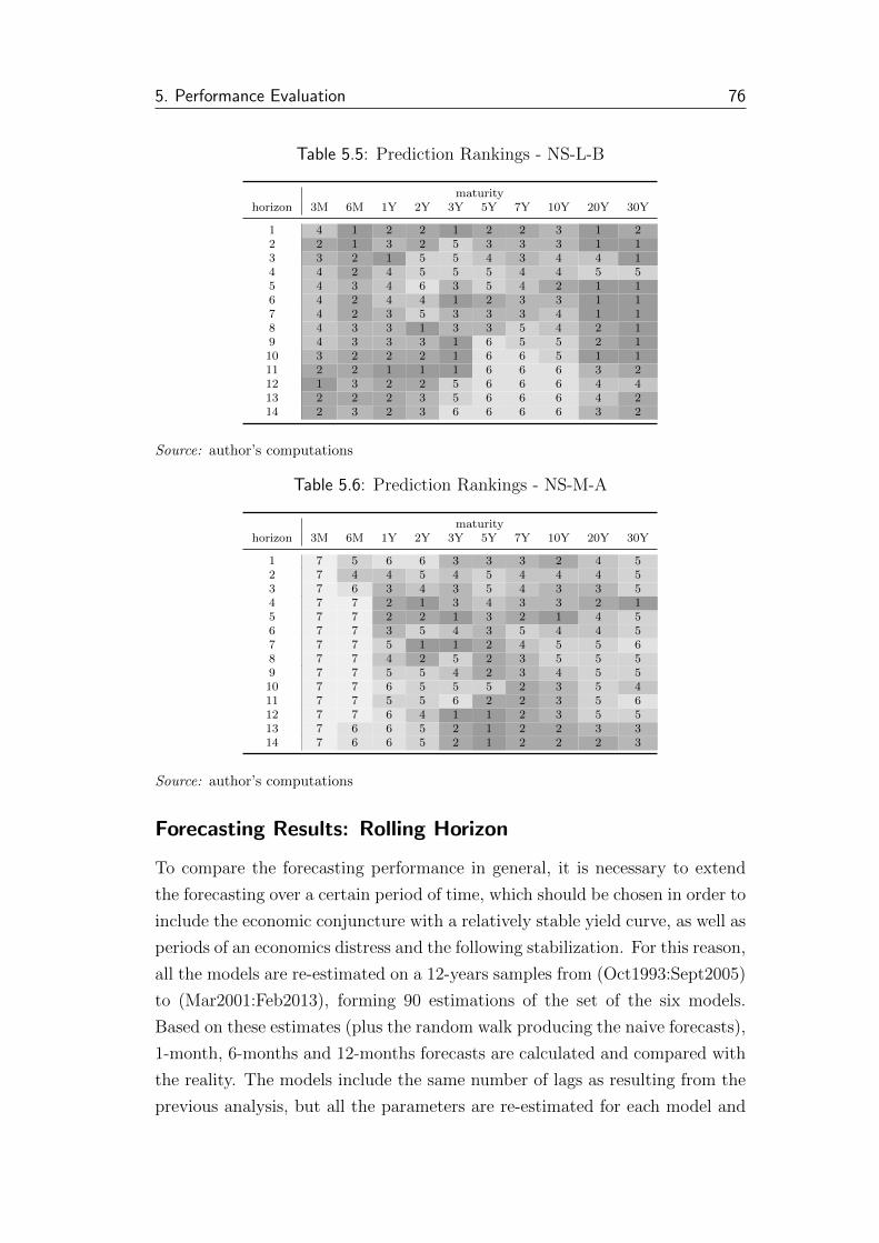
5. Performance Evaluation 76
Table 5.5: Prediction Rankings - NS-L-B
maturityhorizon 3M 6M 1Y 2Y 3Y 5Y 7Y 10Y 20Y 30Y
1 4 1 2 2 1 2 2 3 1 22 2 1 3 2 5 3 3 3 1 13 3 2 1 5 5 4 3 4 4 14 4 2 4 5 5 5 4 4 5 55 4 3 4 6 3 5 4 2 1 16 4 2 4 4 1 2 3 3 1 17 4 2 3 5 3 3 3 4 1 18 4 3 3 1 3 3 5 4 2 19 4 3 3 3 1 6 5 5 2 110 3 2 2 2 1 6 6 5 1 111 2 2 1 1 1 6 6 6 3 212 1 3 2 2 5 6 6 6 4 413 2 2 2 3 5 6 6 6 4 214 2 3 2 3 6 6 6 6 3 2
Source: author’s computations
Table 5.6: Prediction Rankings - NS-M-A
maturityhorizon 3M 6M 1Y 2Y 3Y 5Y 7Y 10Y 20Y 30Y
1 7 5 6 6 3 3 3 2 4 52 7 4 4 5 4 5 4 4 4 53 7 6 3 4 3 5 4 3 3 54 7 7 2 1 3 4 3 3 2 15 7 7 2 2 1 3 2 1 4 56 7 7 3 5 4 3 5 4 4 57 7 7 5 1 1 2 4 5 5 68 7 7 4 2 5 2 3 5 5 59 7 7 5 5 4 2 3 4 5 510 7 7 6 5 5 5 2 3 5 411 7 7 5 5 6 2 2 3 5 612 7 7 6 4 1 1 2 3 5 513 7 6 6 5 2 1 2 2 3 314 7 6 6 5 2 1 2 2 2 3
Source: author’s computations
Forecasting Results: Rolling Horizon
To compare the forecasting performance in general, it is necessary to extend
the forecasting over a certain period of time, which should be chosen in order to
include the economic conjuncture with a relatively stable yield curve, as well as
periods of an economics distress and the following stabilization. For this reason,
all the models are re-estimated on a 12-years samples from (Oct1993:Sept2005)
to (Mar2001:Feb2013), forming 90 estimations of the set of the six models.
Based on these estimates (plus the random walk producing the naive forecasts),
1-month, 6-months and 12-months forecasts are calculated and compared with
the reality. The models include the same number of lags as resulting from the
previous analysis, but all the parameters are re-estimated for each model and

5. Performance Evaluation 77
Table 5.7: Prediction Rankings - NS-M-B
maturityhorizon 3M 6M 1Y 2Y 3Y 5Y 7Y 10Y 20Y 30Y
1 5 2 3 4 4 1 1 4 2 32 6 5 2 3 3 2 2 1 2 33 6 5 4 3 4 2 2 2 1 24 6 6 5 3 4 2 2 2 3 35 6 6 5 1 2 1 1 3 3 36 6 6 5 3 3 6 6 6 3 27 6 6 6 6 2 6 6 6 4 28 6 6 6 5 4 6 6 6 4 39 6 6 7 6 5 5 6 6 3 210 6 6 7 6 6 2 5 4 2 211 6 6 7 7 7 3 5 5 2 312 6 6 7 6 2 3 4 4 3 313 6 7 7 6 4 3 3 4 1 114 6 7 7 7 3 3 3 3 1 1
Source: author’s computations
Table 5.8: Prediction Rankings - AF-L
maturityhorizon 3M 6M 1Y 2Y 3Y 5Y 7Y 10Y 20Y 30Y
1 3 7 4 3 7 7 6 6 6 62 5 7 5 6 7 7 6 6 6 63 4 7 6 6 7 6 5 6 6 64 3 5 6 6 7 6 5 6 6 65 3 5 6 5 6 4 3 5 6 66 3 5 6 2 2 4 4 1 5 67 3 5 4 3 4 4 5 1 2 48 3 5 5 3 1 5 4 2 1 29 3 5 4 2 3 4 4 1 1 310 4 5 4 4 3 4 4 1 3 511 4 5 4 4 4 5 4 2 1 112 5 5 4 1 3 4 3 2 1 113 4 5 3 1 1 4 4 1 2 614 5 5 3 1 1 4 4 1 4 6
Source: author’s computations
period separately6.
From the first view, the results are not much encouraging. Comparing the
Root mean square error (RMSE) calculated over the whole 90 forecasts per each
maturity and forecasting horizon, the random walk7 performs best in almost
all cases, as displays the Table 5.10 showing the total aggregated RMSE over
all maturities (the results are, nevertheless, similar also for the single maturi-
ties). Regardless to this fact, it is obvious, that in case of the Nelson-Siegel
6For the affine models AF-L and AF-M, the number of iterations when numerically com-puting some of the parameters had to be restricted, due to the technical limitations (theauthor has used an ordinary laptop). To estimate these models as precisely as the mainestimation described above, it would require more than four months of a pure computationaltime.
7i.e. naive forecasts set to be equal to the latest observation

5. Performance Evaluation 78
Table 5.9: Prediction Rankings - AF-M
maturityhorizon 3M 6M 1Y 2Y 3Y 5Y 7Y 10Y 20Y 30Y
1 2 6 7 7 6 5 7 7 7 72 1 6 7 7 2 4 7 7 7 73 1 4 7 7 2 3 7 7 7 74 2 3 7 7 1 3 7 7 7 75 2 2 7 7 7 2 6 7 7 76 1 4 7 7 7 5 1 5 7 77 2 3 7 7 7 5 1 3 7 78 1 2 7 7 7 4 1 1 7 79 1 2 6 7 6 3 1 2 7 710 2 4 5 7 4 1 1 6 7 711 3 4 6 6 3 1 1 1 6 512 3 4 5 7 6 2 1 1 2 213 3 4 5 7 6 2 1 3 7 714 3 4 5 6 5 2 1 4 7 7
Source: author’s computations
framework, adding macro-factors leads to on average slightly worse results than
in case of the latent-factors-only models. Moreover, the models based on λB
produce generally more accurate forecasts than these using λA. In case of the
affine models, the macro-extended model AF-M performs generally better than
the AF-L form.
However, when examining the performance in a bigger detail, certain fea-
tures of the predictive dynamics can be identified:
� For the short rate (3M), the naive forecasts (random walk) systematically
outperform the other models only for the period beginning with the fall
of the short rates in 2008 - the situation is captured by the figures 5.1
to 5.3 illustrating the development of the RMSE calculated on a rolling
9-months window. It is not surprising, that at the period of extremely
low (and rather not volatile) short rates, the naive forecasts perform best
(see the Figure 4.3 for a context). However, for the years preceding this
period, the random walk was rarely the best performing model. For 1-
month prediction horizon, the affine models produced the most accurate
forecasts, whereas for longer horizons (6 and 12 months), also the NS-L-A
and NS-L-B were successful, when very closely followed the development
of the AF-L model. Regardless the horizon, the macro-extended Nelson-
Siegel models show the worst performance for the shortest maturity.
� Moving to the middle rates (for example 3Y), the situation is outlined
by figures 5.4-5.6. For these maturities, the performance of AF-L and
AF-M models becomes poor (especially for the shortest horizon), and the

5. Performance Evaluation 79
Nelson-Siegel-based models are usually not able to beat the random walk
as well. The only exception is a period of growing rates during the years
2006 and 2007, when the AF-M model is performing the best.
� Finally, using the graphical illustration also for the longest yields (30Y)
in figures 5.7-5.9, the predictions of the longest rate resulting from all
the models are beating the naive forecasts in periods of changes on the
financial markets related to the change of the market price of risk, whereas
the random walk is performing best in the periods with a relatively stable
situation.
Table 5.10: Predictions - RMSE
modelhorizon RW NS-L-A NS-L-B NS-M-A NS-M-B AF-L AF-M
1 month 0.2510 0.2903 0.2780 0.3354 0.3250 1.0998 0.99976 month 0.7193 0.8451 0.8389 1.1378 1.1350 1.3941 1.280112 month 0.9878 1.2107 1.2032 1.8352 1.8340 1.7167 1.5694
note: RMSE calculated from out-sample periods September 2005 - February 2013.
Source: author’s computations
Figure 5.1: 3M Yields Forecasting: One Month Prediction Horizon
12−2005 12−2006 12−2007 12−2008 12−2009 12−2010 12−2011 12−20120
0.1
0.2
0.3
0.4
0.5
0.6
0.7
0.8
period of prediction
RM
SE
: 9−
perio
ds w
indo
w
random walkNS−L−ANS−L−BNS−M−ANS−M−BAF−LAF−M
Source: author’s computations
5.3 Comparison with Similar Studies
The implications of the forecasting performance evaluation can be well extended
by comparing the results with findings of similar studies, which were already
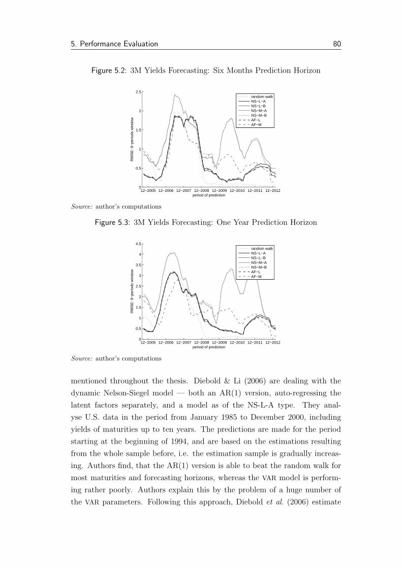
5. Performance Evaluation 80
Figure 5.2: 3M Yields Forecasting: Six Months Prediction Horizon
12−2005 12−2006 12−2007 12−2008 12−2009 12−2010 12−2011 12−20120
0.5
1
1.5
2
2.5
period of prediction
RM
SE
: 9−
perio
ds w
indo
w
random walkNS−L−ANS−L−BNS−M−ANS−M−BAF−LAF−M
Source: author’s computations
Figure 5.3: 3M Yields Forecasting: One Year Prediction Horizon
12−2005 12−2006 12−2007 12−2008 12−2009 12−2010 12−2011 12−20120
0.5
1
1.5
2
2.5
3
3.5
4
4.5
period of prediction
RM
SE
: 9−
perio
ds w
indo
w
random walkNS−L−ANS−L−BNS−M−ANS−M−BAF−LAF−M
Source: author’s computations
mentioned throughout the thesis. Diebold & Li (2006) are dealing with the
dynamic Nelson-Siegel model — both an AR(1) version, auto-regressing the
latent factors separately, and a model as of the NS-L-A type. They anal-
yse U.S. data in the period from January 1985 to December 2000, including
yields of maturities up to ten years. The predictions are made for the period
starting at the beginning of 1994, and are based on the estimations resulting
from the whole sample before, i.e. the estimation sample is gradually increas-
ing. Authors find, that the AR(1) version is able to beat the random walk for
most maturities and forecasting horizons, whereas the VAR model is perform-
ing rather poorly. Authors explain this by the problem of a huge number of
the VAR parameters. Following this approach, Diebold et al. (2006) estimate

5. Performance Evaluation 81
Figure 5.4: 3Y Yields Forecasting: One Month Prediction Horizon
12−2005 12−2006 12−2007 12−2008 12−2009 12−2010 12−2011 12−20120
0.5
1
1.5
2
2.5
period of prediction
RM
SE
: 9−
perio
ds w
indo
w
random walkNS−L−ANS−L−BNS−M−ANS−M−BAF−LAF−M
Source: author’s computations
Figure 5.5: 3Y Yields Forecasting: Six Months Prediction Horizon
12−2005 12−2006 12−2007 12−2008 12−2009 12−2010 12−2011 12−20120
0.5
1
1.5
2
2.5
period of prediction
RM
SE
: 9−
perio
ds w
indo
w
random walkNS−L−ANS−L−BNS−M−ANS−M−BAF−LAF−M
Source: author’s computations
the dynamic Nelson-Siegel model with the state variables vector enriched by
macroeconomic variables, forming a NS-M-A model. Authors do not examine
forecasting ability of the model, but conclude that the macroeconomic variables
have a strong impact on future yields.
Ang & Piazzesi (2003) use a much longer period — from June 1952 to De-
cember 2000, including maturities up to five years. Moreover, authors repre-
sent the macroeconomic situation by variables constructed as the first principal
components of two groups of macroeconomic variables, called inflation and real
activity. Based on the data, the models similar to AF-L and AF-M are created
(using a maximum likelihood method). Forecasting is made one step ahead,
and its results are following: for the maturity 3 months, the naive forecasts are
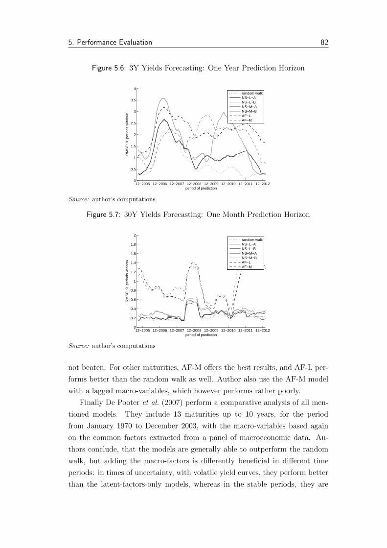
5. Performance Evaluation 82
Figure 5.6: 3Y Yields Forecasting: One Year Prediction Horizon
12−2005 12−2006 12−2007 12−2008 12−2009 12−2010 12−2011 12−20120
0.5
1
1.5
2
2.5
3
3.5
4
period of prediction
RM
SE
: 9−
perio
ds w
indo
w
random walkNS−L−ANS−L−BNS−M−ANS−M−BAF−LAF−M
Source: author’s computations
Figure 5.7: 30Y Yields Forecasting: One Month Prediction Horizon
12−2005 12−2006 12−2007 12−2008 12−2009 12−2010 12−2011 12−20120
0.2
0.4
0.6
0.8
1
1.2
1.4
1.6
1.8
2
period of prediction
RM
SE
: 9−
perio
ds w
indo
w
random walkNS−L−ANS−L−BNS−M−ANS−M−BAF−LAF−M
Source: author’s computations
not beaten. For other maturities, AF-M offers the best results, and AF-L per-
forms better than the random walk as well. Author also use the AF-M model
with a lagged macro-variables, which however performs rather poorly.
Finally De Pooter et al. (2007) perform a comparative analysis of all men-
tioned models. They include 13 maturities up to 10 years, for the period
from January 1970 to December 2003, with the macro-variables based again
on the common factors extracted from a panel of macroeconomic data. Au-
thors conclude, that the models are generally able to outperform the random
walk, but adding the macro-factors is differently beneficial in different time
periods: in times of uncertainty, with volatile yield curves, they perform better
than the latent-factors-only models, whereas in the stable periods, they are
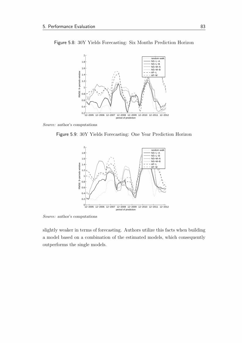
5. Performance Evaluation 83
Figure 5.8: 30Y Yields Forecasting: Six Months Prediction Horizon
12−2005 12−2006 12−2007 12−2008 12−2009 12−2010 12−2011 12−20120.2
0.4
0.6
0.8
1
1.2
1.4
1.6
1.8
2
period of prediction
RM
SE
: 9−
perio
ds w
indo
w
random walkNS−L−ANS−L−BNS−M−ANS−M−BAF−LAF−M
Source: author’s computations
Figure 5.9: 30Y Yields Forecasting: One Year Prediction Horizon
12−2005 12−2006 12−2007 12−2008 12−2009 12−2010 12−2011 12−20120
0.2
0.4
0.6
0.8
1
1.2
1.4
1.6
1.8
2
period of prediction
RM
SE
: 9−
perio
ds w
indo
w
random walkNS−L−ANS−L−BNS−M−ANS−M−BAF−LAF−M
Source: author’s computations
slightly weaker in terms of forecasting. Authors utilize this facts when building
a model based on a combination of the estimated models, which consequently
outperforms the single models.

Chapter 6
Conclusion
The thesis compares various approaches to the term structure of interest rates
modelling, focusing on the macro-finance models. The work is concerned with
capturing the real-world dynamics of the interest rates, with emphasis given to
the estimated models properties and a forecasting performance. Two widely-
used groups of models are first described: a dynamic Nelson-Siegel framework
and an affine class of models. Afterwards, the models are exactly specified
in several different ways, deriving both latent-factors-only and macro-finance
version for each of the groups of models. Moreover, the Nelson-Siegel based
models also vary by the two different ways to obtaining the fit-parameter λ.
A naıve model — the random walk — is used as a benchmark, as it produces
naive forecasts equal to the latest observation.
After the models are estimated on U.S. data, the estimation results show,
that the in-sample fit is better for the Nelson-Siegel based models as compared
to the affine models, mainly because of the parsimony of these models. How-
ever, it is shown that the models can be regarded as complementary, since the
latent factor representing the level of the yield curve is specified differently in
both cases — this is supported by an inspection of impulse responses result-
ing from the models, which are in line with both macroeconomic and financial
reality. An important implication from the impulse responses is also the fact,
that the explicit inclusion of the macroeconomic variables allows to examine
the impact of the macroeconomic variables on different parts of the yield curve.
The forecasts are performed in two ways — first, results of the estimated
models are used to create predictions for the most recent period, which is
then compared to the reality. It is shown, that the naive forecasts are not
outperformed for both shortest maturities and shortest prediction horizons —

6. Conclusion 85
except for the ability of the macro-extended affine model to beat the naive
forecasts in some cases. However, for longer maturities (above two years) and
a longer prediction horizon (more then four months), most of the estimated
models predict better than the naıve approach. Moreover, adding macro-factors
is rather beneficial for the affine models, whereas worsens results of the Nelson-
Siegel-based predictions. A certain complementarity of the models is again
present. Second, the models are re-estimated based on a rolling in-sample, with
forecasts resulting from them. Summing the results, the random walk performs
the best, followed by the Nelson-Siegel model, with the affine models performing
the worst. However, when focusing on the time-development of the forecasting
accuracy, the random walk is outperformed frequently, depending on the actual
conditions: For the shortest-maturity yields, the models are successful except
for the extremely low short rates as since the year 2009. Contrary, for the
longest maturities, the models are able to predict the reality well especially in
the times of changes on financial markets, with varying market price of risk.
As compared to similar studies, the biggest benefits of the thesis are fol-
lowing: First, maturities longer than 10 years are included, and the estimated
models are able to both capture their dynamics and produce reasonable fore-
casts. Second, it is shown that the dynamic Nelson-Siegel and affine models are
complementary into a significant extent, both of them performing differently
under various market and economic conditions; moreover, adding the macro-
factors is more beneficial for the affine models than for the Nelson-Siegel-based.
Third, it has been illustrated, that the fit-parameter of the dynamic Nelson-
Siegel model, based on an optimal in-sample fit, offers better predictive re-
sults as compared to the parameter value ensuring the optimal curvature of
the yield curve. Finally, the models were estimated on the most recent data,
which makes them stable in terms of structural changes and — since they try
to explain macroeconomic relations — can be regarded as resisting the Lucas
Critique. Consequently, the estimated relations of the variables, implying a
weak impact of the monetary policy steps on the longest maturities, can be
considered as generally valid.
In many cases, the analysis could be further extended. Different models
could be included into the analysis, for example a DSGE model with a term
structure specification, which would make the comparison more comprehen-
sive. Focusing on the included models, a different approach to the affine model
estimation could be used, particularly solving the difficulties related to the
numerical procedures.
Bibliography
Ang, A. & M. Piazzesi (2003): “A No-Arbitrage Vector Autoregression of
Term Structure Dynamics with Macroeconomic and Latent Variables.” Jour-
nal of Monetary Economics 50: p. 745–787.
Ang, A., M. Piazzesi, & M. Wei (2006): “What does the Yield Curve tell us
about GDP Growth?” Journal of Econometrics 131: p. 359–403.
Box, G. & G. Jenkins (1970): Time Series Analysis, Forecasting and Control.
San Francisco: Holden-Day.
Brace, A., D. Gatarek, & M. Musiela (1997): “The Market Model of
Interest Rates Dynamics.” Mathematical Finance 7: pp. 127–154.
Choudhry, M. (2011): Analysing and Interpreting the Yield Curve. Hoboken,
NJ, USA: Wiley.
Cox, J. C., J. E. Ingersoll, & S. A. Ross (1985): “A Theory of the Term
Structure of Interest Rates.” Econometrica 53(2): pp. 385–408.
Culberison, J. M. (1957): “The Term Structure of Interest Rates.” Quarterly
Journal of Economics 71: pp. 485–517.
De Pooter, M., F. Ravazzolo, & D. van Dijk (2007): “Predicting the
Term Structure of Interest Rates: Incorporating parameter uncertainty,
model uncertainty and macroeconomic information.” Technical Report TI
07-028/4, T.
Diebold, F. X. & C. Li (2006): “Forecasting the Term Structure of Govern-
ment Bond Yields.” Journal of Econometrics 130: pp. 337–364.
Diebold, F. X., G. D. Rudebusch, & S. B. Aruoba (2006): “The Macroe-
conomy and the Yield Curve: A Dynamic Latent Factor Approach.” Journal
of Econometrics 131: pp. 309–338.

Bibliography 87
Downes, J. & J. Goodman (1998): Dictionary of Finance and Investment
Terms. New York: Barron’s Educational Series, fifth edition.
Duffee, G. R. (2002): “Term Premia and Interest Rate Forecasts in Affine
Models.” The Journal of Finance 57(1): pp. 405–443.
Duffie, G. & R. Kan (1996): “A Yield-Factor Model of Interest Rates.”
Mathematical Finance 6: pp. 379–406.
Fama, E. F. (1965): “Random Walks In Stock Market Prices.” Financial
Analysts Journal 21(5): pp. 55–59.
Fama, E. F. (1970): “Efficient Capital Markets: A Review of Theory and
Empirical Work.” The Journal of Finance 25: p. 383–417.
FED (2014): “Federal Reserve statistical release - H.15 (519) Selected In-
terest Rates.” Statistical release, Board of Governors of the Federal Re-
serve System . [Online], accessed 20-March-2014. Available at http://www.
federalreserve.gov/releases/h15/current/h15.pdf.
Filipovic, D. (2009): Term-Structure Models: A Graduate Course. Springer,
Springer Finance edition.
Fong, H. G. & O. Vasicek (1991): “Fixed-income Volatility Management.”
The Journal of Portfolio Management 17(4): pp. 41–56.
FRED (2014): “Federal Reserve Economic Data.” Online database, Federal
Reserve Board of St. Louis. [Online], accessed 19-March-2014. Available at
http://research.stlouisfed.org/fred2/.
Gisiger, N. (2010): “Risk-Neutral Probabilities Explained.” Technical report,
University of Zurich. Lecture notes for master program MSc UZH ETH in
Quantitative Finance.
Haugh, M. (2010): “Introduction to Stochastic Calculus.” Technical report,
Columbia Universtity in the City of New York. Lecture notes for master
program Financial Engineering, lecture Continuous-Time Models.
Heath, D., R. Jarrow, & A. Morton (1992): “Bond Pricing and the Term
Structure of Interest Rates.” Econometrica 60: pp. 77–106.
Hicks, J. R. (1946): Value and Capital. London: Oxford University Press, 2nd
edition.

Bibliography 88
Ho, T. & S. Lee (1986): “Term Structure Movements and Pricing Interest
Claims.” Journal of Finance 41: pp. 1011–1029.
Hull, J. C. & A. D. White (1990): “Pricing Interest Rate Derivative Securi-
ties.” The Review of Financial Studies 3(4): p. 573–592.
Kalman, R. E. (1960): “A New Approach to Linear Filtering and Predic-
tion Problems.” Transactions of the ASME – Journal of Basic Engineering
82(Series D): pp. 35–45.
Kladıvko, K. (2011): Interest Rate Modeling. Ph.D. Thesis, University of
Economics, Prague.
Kollar, M. (2011): Macrofinance Modeling from Asset Allocation Perspective.
Ph.D. Thesis, University of Economics, Prague.
Litterman, R. & J. Scheinkman (1991): “Common Factors Affecting Bond
Returns.” The Journal of Fixed Income 1(1): pp. 54–61.
Lucas, R. J. (1976): “Econometric policy evaluation: A critique.” Carnegie-
Rochester Conference Series on Public Policy 1(1): pp. 19–46.
Malek, J. (2005): Dynamika urokovych mer a urokove derivaty. Praha: Eko-
press.
Monch, E. (2006): “Forecasting the Yield Curve in a Data-Rich Environ-
ment: A No-Arbitrage Factor-Augmented VAR Approach.” Working paper,
Humboldt University Berlin, Berlin.
Modigliani, F. & R. Sutch (1966): “Innovations in Interest Rate Policy.”
American Economic Review 56: pp. 178–197.
Musiela, M. & M. Rutkowski (2005): Martingale Methods in Financial
Modelling. Springer.
Nelson, C. R. & A. F. Siegel (1987): “Parsimonious Modeling of Yield
Curves.” Journal of Business 60(4): pp. 473–489.
Piazzesi, M. (2009): “Affine Term Structure Models.” In Y. Ait-Sahalia
& L. Hansen (editors), “Handbook of Financial Econometrics,” volume 1,
chapter 12. Elsevier.
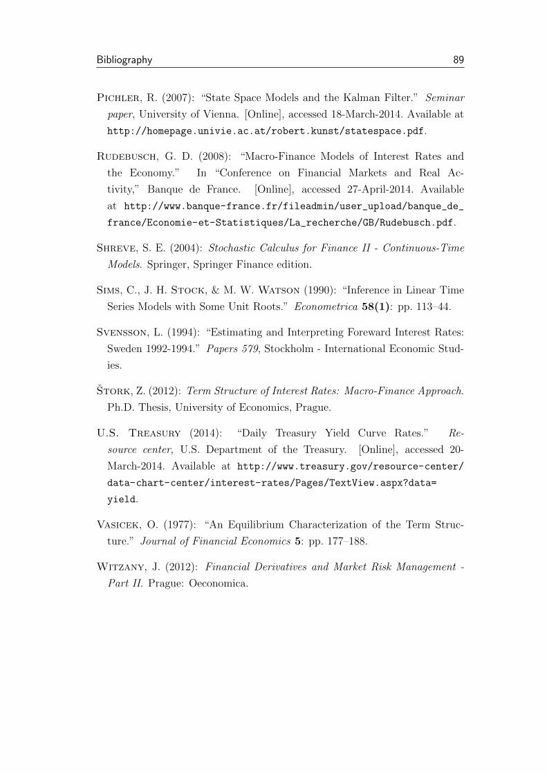
Bibliography 89
Pichler, R. (2007): “State Space Models and the Kalman Filter.” Seminar
paper, University of Vienna. [Online], accessed 18-March-2014. Available at
http://homepage.univie.ac.at/robert.kunst/statespace.pdf.
Rudebusch, G. D. (2008): “Macro-Finance Models of Interest Rates and
the Economy.” In “Conference on Financial Markets and Real Ac-
tivity,” Banque de France. [Online], accessed 27-April-2014. Available
at http://www.banque-france.fr/fileadmin/user_upload/banque_de_
france/Economie-et-Statistiques/La_recherche/GB/Rudebusch.pdf.
Shreve, S. E. (2004): Stochastic Calculus for Finance II - Continuous-Time
Models. Springer, Springer Finance edition.
Sims, C., J. H. Stock, & M. W. Watson (1990): “Inference in Linear Time
Series Models with Some Unit Roots.” Econometrica 58(1): pp. 113–44.
Svensson, L. (1994): “Estimating and Interpreting Foreward Interest Rates:
Sweden 1992-1994.” Papers 579, Stockholm - International Economic Stud-
ies.
Stork, Z. (2012): Term Structure of Interest Rates: Macro-Finance Approach.
Ph.D. Thesis, University of Economics, Prague.
U.S. Treasury (2014): “Daily Treasury Yield Curve Rates.” Re-
source center, U.S. Department of the Treasury. [Online], accessed 20-
March-2014. Available at http://www.treasury.gov/resource-center/
data-chart-center/interest-rates/Pages/TextView.aspx?data=
yield.
Vasicek, O. (1977): “An Equilibrium Characterization of the Term Struc-
ture.” Journal of Financial Economics 5: pp. 177–188.
Witzany, J. (2012): Financial Derivatives and Market Risk Management -
Part II. Prague: Oeconomica.

Appendix A
Estimated Parameters
NS-L-A
Figure A.1: NS-L-A estimation results
34
56
78
Diagram of fit and residuals for beta1A
0 50 100 150 200
−1.
00.
00.
5
0 2 4 6 8 10 12
0.0
0.8
Lag
ACF Residuals
2 4 6 8 10 12
−0.
10.
2
Lag
PACF Residuals
−5
−3
−1
1
Diagram of fit and residuals for beta2A
0 50 100 150 200
−1.
00.
00.
5
0 2 4 6 8 10 12
0.0
0.8
Lag
ACF Residuals
2 4 6 8 10 12
−0.
10
Lag
PACF Residuals
−6
−2
02
Diagram of fit and residuals for beta3A
0 50 100 150 200
−2
−1
01
2
0 2 4 6 8 10 12
−0.
20.
8
Lag
ACF Residuals
2 4 6 8 10 12
−0.
20.
1
Lag
PACF Residuals
Source: author’s computations

A. Estimated Parameters II
Table A.1: Estimation results for equation beta1A:
Estimate Std. Error t value Pr(> |t|)
beta1A.l1 1.0139933 0.1073265 9.448 < 2e-16beta2A.l1 0.0015088 0.0791861 0.019 0.9848beta3A.l1 0.0133321 0.0226547 0.588 0.5568beta1A.l2 -0.2488234 0.1488980 -1.671 0.0962beta2A.l2 0.0755234 0.1116589 0.676 0.4995beta3A.l2 -0.0150110 0.0324617 -0.462 0.6443beta1A.l3 0.2426650 0.1491001 1.628 0.1051beta2A.l3 -0.1536011 0.1140515 -1.347 0.1795beta3A.l3 -0.0294117 0.0325206 -0.904 0.3668beta1A.l4 -0.1854988 0.1031092 -1.799 0.0734beta2A.l4 0.0665581 0.0749128 0.888 0.3753beta3A.l4 0.0272309 0.0249150 1.093 0.2756const 1.2808763 0.3087691 4.148 4.84e-05trend -0.0030140 0.0007073 -4.261 3.05e-05
Source: R-studio, author’s computations
Table A.2: Estimation results for equation beta2A:
Estimate Std. Error t value Pr(> |t|)
beta1A.l1 -0.0361915 0.1484708 -0.244 0.8076beta2A.l1 0.9732143 0.1095425 8.884 2.73e-16beta3A.l1 0.0675338 0.0313395 2.155 0.0323beta1A.l2 0.4960026 0.2059790 2.408 0.0169beta2A.l2 0.1575704 0.1544639 1.020 0.3088beta3A.l2 0.0479330 0.0449060 1.067 0.2870beta1A.l3 -0.4426866 0.2062584 -2.146 0.0330beta2A.l3 -0.0194332 0.1577738 -0.123 0.9021beta3A.l3 -0.0751986 0.0449876 -1.672 0.0961beta1A.l4 0.0730462 0.1426367 0.512 0.6091beta2A.l4 -0.1729574 0.1036310 -1.669 0.0966beta3A.l4 0.0186514 0.0344663 0.541 0.5890const -0.7834363 0.4271375 -1.834 0.0680trend 0.0024783 0.0009785 2.533 0.0120
Source: R-studio, author’s computations

A. Estimated Parameters III
Table A.3: Estimation results for equation beta3A:
Estimate Std. Error t value Pr(> |t|)
beta1A.l1 1.087963 0.325185 3.346 0.00097beta2A.l1 0.721926 0.239923 3.009 0.00294beta3A.l1 0.944119 0.068641 13.755 < 2e-16beta1A.l2 -1.224839 0.451141 -2.715 0.00717beta2A.l2 -0.895088 0.338311 -2.646 0.00876beta3A.l2 -0.146735 0.098354 -1.492 0.13721beta1A.l3 -0.016959 0.451753 -0.038 0.97009beta2A.l3 0.032708 0.345561 0.095 0.92468beta3A.l3 0.207122 0.098533 2.102 0.03672beta1A.l4 0.106531 0.312407 0.341 0.73344beta2A.l4 0.238280 0.226976 1.050 0.29500beta3A.l4 -0.173485 0.075489 -2.298 0.02252const 0.658438 0.935528 0.704 0.48232trend -0.004781 0.002143 -2.231 0.02674
Source: R-studio, author’s computations

A. Estimated Parameters IV
NS-L-B
Figure A.2: NS-L-B estimation results3
45
67
8
Diagram of fit and residuals for beta1B
0 50 100 150 200
−1.
0−
0.5
0.0
0.5
0 2 4 6 8 10 12
0.0
0.8
Lag
ACF Residuals
2 4 6 8 10 12
−0.
10
Lag
PACF Residuals
−5
−3
−1
Diagram of fit and residuals for beta2B
0 50 100 150 200
−1.
00.
00.
50 2 4 6 8 10 12
0.0
0.8
Lag
ACF Residuals
2 4 6 8 10 12
−0.
10
Lag
PACF Residuals
−6
−2
02
4
Diagram of fit and residuals for beta3B
0 50 100 150 200
−2
−1
01
2
0 2 4 6 8 10 12
0.0
0.8
Lag
ACF Residuals
2 4 6 8 10 12
−0.
10
Lag
PACF Residuals
Source: author’s computations

A. Estimated Parameters V
Table A.4: Estimation results for equation beta1B:
Estimate Std. Error t value Pr(> |t|)
beta1B.l1 0.9758961 0.1056927 9.233 < 2e-16beta2B.l1 -0.0112432 0.0780282 -0.144 0.8856beta3B.l1 0.0178910 0.0216349 0.827 0.4092beta1B.l2 -0.2056409 0.1468627 -1.400 0.1629beta2B.l2 0.0903262 0.1128790 0.800 0.4245beta3B.l2 -0.0278579 0.0300483 -0.927 0.3549beta1B.l3 0.2326543 0.1470977 1.582 0.1152beta2B.l3 -0.1627541 0.1150401 -1.415 0.1586beta3B.l3 -0.0132403 0.0300067 -0.441 0.6595beta1B.l4 -0.1851969 0.1013710 -1.827 0.0691beta2B.l4 0.0677670 0.0754446 0.898 0.3701beta3B.l4 0.0229792 0.0231778 0.991 0.3226const 1.2980557 0.3085908 4.206 3.82e-05trend -0.0028650 0.0006945 -4.125 5.31e-05
Source: R-studio, author’s computations
Table A.5: Estimation results for equation beta2B:
Estimate Std. Error t value Pr(> |t|)
beta1B.l1 0.059199 0.145493 0.407 0.6845beta2B.l1 1.058078 0.107411 9.851 <2e-16beta3B.l1 0.060664 0.029782 2.037 0.0429beta1B.l2 0.396035 0.202166 1.959 0.0514beta2B.l2 0.100679 0.155385 0.648 0.5177beta3B.l2 0.043377 0.041363 1.049 0.2955beta1B.l3 -0.441115 0.202489 -2.178 0.0305beta2B.l3 -0.040605 0.158360 -0.256 0.7979beta3B.l3 -0.074092 0.041306 -1.794 0.0743beta1B.l4 0.077945 0.139544 0.559 0.5770beta2B.l4 -0.152191 0.103854 -1.465 0.1443beta3B.l4 0.017502 0.031906 0.549 0.5839const -0.755286 0.424795 -1.778 0.0768trend 0.002067 0.000956 2.162 0.0318
Source: R-studio, author’s computations
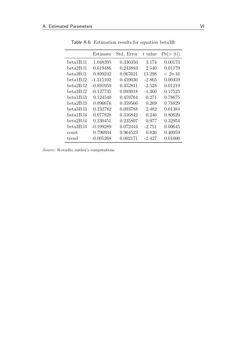
A. Estimated Parameters VI
Table A.6: Estimation results for equation beta3B:
Estimate Std. Error t value Pr(> |t|)
beta1B.l1 1.048395 0.330350 3.174 0.00173beta2B.l1 0.619486 0.243883 2.540 0.01179beta3B.l1 0.899242 0.067621 13.298 < 2e-16beta1B.l2 -1.315102 0.459030 -2.865 0.00459beta2B.l2 -0.891959 0.352811 -2.528 0.01219beta3B.l2 -0.127735 0.093918 -1.360 0.17525beta1B.l3 0.124540 0.459764 0.271 0.78675beta2B.l3 0.096676 0.359566 0.269 0.78829beta3B.l3 0.232782 0.093788 2.482 0.01384beta1B.l4 0.077828 0.316842 0.246 0.80620beta2B.l4 0.230451 0.235807 0.977 0.32954beta3B.l4 -0.199289 0.072444 -2.751 0.00645const 0.796934 0.964523 0.826 0.40959trend -0.005268 0.002171 -2.427 0.01606
Source: R-studio, author’s computations

A. Estimated Parameters VII
NS-M-A
Figure A.3: NS-M-A estimation results - latent variables3
45
67
8
Diagram of fit and residuals for beta1A
0 50 100 150 200
−0.
50.
00.
5
0 2 4 6 8 10 12
0.0
0.8
Lag
ACF Residuals
2 4 6 8 10 12
−0.
10
Lag
PACF Residuals
−5
−3
−1
1
Diagram of fit and residuals for beta2A
0 50 100 150 200
−1.
00.
00.
50 2 4 6 8 10 12
0.0
0.8
Lag
ACF Residuals
2 4 6 8 10 12
−0.
10
Lag
PACF Residuals
−6
−2
02
Diagram of fit and residuals for beta3A
0 50 100 150 200
−2
−1
01
2
0 2 4 6 8 10 12
0.0
0.8
Lag
ACF Residuals
2 4 6 8 10 12
−0.
10
Lag
PACF Residuals
Source: author’s computations
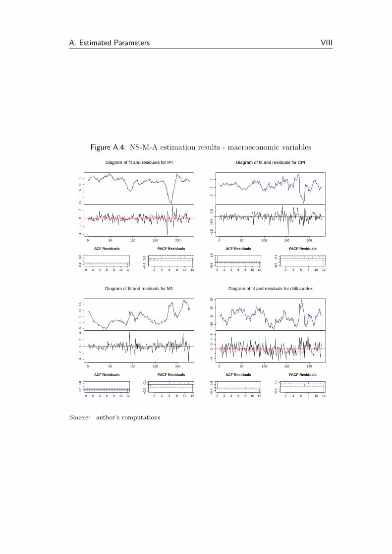
A. Estimated Parameters VIII
Figure A.4: NS-M-A estimation results - macroeconomic variables
−15
−5
05
Diagram of fit and residuals for IPI
0 50 100 150 200
−4
−2
02
0 2 4 6 8 10 12
−0.
40.
8
Lag
ACF Residuals
2 4 6 8 10 12
−0.
40.
0
Lag
PACF Residuals
02
4
Diagram of fit and residuals for CPI
0 50 100 150 200
−1.
5−
0.5
0.5
0 2 4 6 8 10 12
−0.
51.
0
Lag
ACF Residuals
2 4 6 8 10 12
−0.
50.
1Lag
PACF Residuals
−5
05
1015
Diagram of fit and residuals for M1
0 50 100 150 200
−4
−2
02
4
0 2 4 6 8 10 12
−0.
20.
8
Lag
ACF Residuals
2 4 6 8 10 12
−0.
30.
1
Lag
PACF Residuals
−10
010
20
Diagram of fit and residuals for dollar.index
0 50 100 150 200
−4
02
46
0 2 4 6 8 10 12
−0.
40.
8
Lag
ACF Residuals
2 4 6 8 10 12
−0.
40.
1
Lag
PACF Residuals
Source: author’s computations

A. Estimated Parameters IX
Table A.7: Estimation results for equation beta1A:
Estimate Std. Error t value Pr(> |t|)
beta1A.l1 1.065027 0.1157 9.205 <2e-16beta2A.l1 0.035073 0.087973 0.399 0.691beta3A.l1 0.036911 0.025172 1.466 0.144IPI.l1 -0.009958 0.021934 -0.454 0.65CPI.l1 -0.046912 0.052032 -0.902 0.368M1.l1 0.007334 0.016312 0.45 0.653dollar.index.l1 -0.003408 0.008401 -0.406 0.685beta1A.l2 -0.247524 0.159861 -1.548 0.123beta2A.l2 0.062193 0.120247 0.517 0.606beta3A.l2 -0.02725 0.035542 -0.767 0.444IPI.l2 0.013891 0.030797 0.451 0.652CPI.l2 0.041725 0.086345 0.483 0.629M1.l2 -0.024121 0.021408 -1.127 0.261dollar.index.l2 0.005681 0.012826 0.443 0.658beta1A.l3 0.280313 0.160372 1.748 0.082beta2A.l3 -0.112353 0.124705 -0.901 0.369beta3A.l3 -0.022411 0.035872 -0.625 0.533IPI.l3 -0.031735 0.030767 -1.031 0.304CPI.l3 -0.077255 0.085515 -0.903 0.367M1.l3 0.002024 0.021352 0.095 0.925dollar.index.l3 -0.01127 0.012811 -0.88 0.38beta1A.l4 -0.105135 0.114033 -0.922 0.358beta2A.l4 0.042888 0.085497 0.502 0.616beta3A.l4 0.002353 0.028272 0.083 0.934IPI.l4 0.023985 0.021924 1.094 0.275CPI.l4 0.042448 0.052751 0.805 0.422M1.l4 0.012842 0.015517 0.828 0.409dollar.index.l4 0.010244 0.008405 1.219 0.224const 0.181851 0.202665 0.897 0.371
Source: R-studio, author’s computations

A. Estimated Parameters X
Table A.8: Estimation results for equation beta2A:
Estimate Std. Error t value Pr(> |t|)
beta1A.l1 -0.1425564 0.1541078 -0.925 0.3561beta2A.l1 0.836459 0.1171756 7.139 1.75e-12beta3A.l1 0.0373072 0.0335278 1.113 0.2672IPI.l1 0.0337623 0.0292157 1.156 0.2492CPI.l1 0.0069091 0.0693049 0.1 0.9207M1.l1 -0.0068317 0.0217275 -0.314 0.7535dollar.index.l1 0.0040184 0.0111895 0.359 0.7199beta1A.l2 0.4940774 0.2129275 2.32 0.0213beta2A.l2 0.175288 0.1601633 1.094 0.2751beta3A.l2 0.0695838 0.0473405 1.47 0.1432IPI.l2 -0.0191166 0.0410205 -0.466 0.6417CPI.l2 -0.0899581 0.115008 -0.782 0.435M1.l2 0.0187666 0.0285144 0.658 0.5112dollar.index.l2 -0.0224014 0.0170836 -1.311 0.1913beta1A.l3 -0.4416754 0.213608 -2.068 0.04beta2A.l3 -0.0395218 0.1661017 -0.238 0.8122beta3A.l3 -0.0654249 0.0477803 -1.369 0.1725IPI.l3 0.0119574 0.0409809 0.292 0.7708CPI.l3 0.1269091 0.1139026 1.114 0.2665M1.l3 -0.007893 0.0284401 -0.278 0.7817dollar.index.l3 0.0263026 0.0170635 1.541 0.1248beta1A.l4 -0.0002758 0.1518876 -0.002 0.9986beta2A.l4 -0.0927531 0.1138781 -0.814 0.4163beta3A.l4 0.0487715 0.0376567 1.295 0.1968IPI.l4 -0.0048517 0.0292016 -0.166 0.8682CPI.l4 -0.0230025 0.0702622 -0.327 0.7437M1.l4 0.0013997 0.0206676 0.068 0.9461dollar.index.l4 -0.0130001 0.011195 -1.161 0.2469const 0.3054586 0.2699415 1.132 0.2592
Source: R-studio, author’s computations

A. Estimated Parameters XI
Table A.9: Estimation results for equation beta3A:
Estimate Std. Error t value Pr(> |t|)
beta1A.l1 1.25265 0.34049 3.679 0.000302beta2A.l1 0.80542 0.25889 3.111 0.00214beta3A.l1 0.98882 0.07408 13.348 <2e-16IPI.l1 -0.08226 0.06455 -1.274 0.204046CPI.l1 -0.18127 0.15313 -1.184 0.2379M1.l1 -0.02129 0.04801 -0.444 0.657853dollar.index.l1 -0.03766 0.02472 -1.523 0.12925beta1A.l2 -1.06897 0.47045 -2.272 0.024148beta2A.l2 -0.95125 0.35387 -2.688 0.007797beta3A.l2 -0.21673 0.1046 -2.072 0.039556IPI.l2 0.12619 0.09063 1.392 0.165375CPI.l2 0.20698 0.2541 0.815 0.416306M1.l2 0.06754 0.063 1.072 0.285018dollar.index.l2 0.07039 0.03775 1.865 0.063668beta1A.l3 -0.04039 0.47196 -0.086 0.931895beta2A.l3 0.17602 0.36699 0.48 0.63202beta3A.l3 0.26271 0.10557 2.489 0.013652IPI.l3 -0.11084 0.09055 -1.224 0.222366CPI.l3 0.01265 0.25166 0.05 0.959947M1.l3 -0.084 0.06284 -1.337 0.182849dollar.index.l3 -0.07183 0.0377 -1.905 0.058181beta1A.l4 0.11242 0.33559 0.335 0.737991beta2A.l4 0.13048 0.25161 0.519 0.60462beta3A.l4 -0.21199 0.0832 -2.548 0.011595IPI.l4 0.05798 0.06452 0.899 0.369927CPI.l4 0.02698 0.15524 0.174 0.862193M1.l4 0.04971 0.04566 1.089 0.277695dollar.index.l4 0.03374 0.02473 1.364 0.174036const -1.62638 0.59642 -2.727 0.006968
Source: R-studio, author’s computations

A. Estimated Parameters XII
Table A.10: Estimation results for equation IPI-A:
Estimate Std. Error t value Pr(> |t|)
beta1A.l1 -0.413094 0.38005 -1.087 0.27838beta2A.l1 -0.269675 0.288971 -0.933 0.35184beta3A.l1 0.09593 0.082684 1.16 0.24736IPI.l1 0.932933 0.07205 12.948 <2e-16CPI.l1 0.184864 0.170915 1.082 0.28074M1.l1 -0.007979 0.053583 -0.149 0.88177dollar.index.l1 0.03897 0.027595 1.412 0.15946beta1A.l2 1.0092 0.525107 1.922 0.05605beta2A.l2 0.688533 0.394984 1.743 0.08285beta3A.l2 0.103409 0.116748 0.886 0.37683IPI.l2 0.204581 0.101162 2.022 0.04449CPI.l2 -0.344505 0.283625 -1.215 0.22595M1.l2 -0.043635 0.07032 -0.621 0.53563dollar.index.l2 -0.093862 0.04213 -2.228 0.02701beta1A.l3 -0.467053 0.526786 -0.887 0.37636beta2A.l3 -0.104953 0.409629 -0.256 0.79805beta3A.l3 -0.103243 0.117833 -0.876 0.38199IPI.l3 0.023824 0.101064 0.236 0.81388CPI.l3 0.245826 0.280899 0.875 0.38256M1.l3 -0.017421 0.070137 -0.248 0.80409dollar.index.l3 0.004411 0.042081 0.105 0.91662beta1A.l4 -0.049085 0.374575 -0.131 0.89587beta2A.l4 -0.295727 0.280839 -1.053 0.29362beta3A.l4 -0.094926 0.092867 -1.022 0.30794IPI.l4 -0.2113 0.072015 -2.934 0.00374CPI.l4 -0.227622 0.173276 -1.314 0.19049M1.l4 0.080779 0.050969 1.585 0.11459dollar.index.l4 0.053167 0.027608 1.926 0.05557const 0.03441 0.665712 0.052 0.95883
Source: R-studio, author’s computations
A. Estimated Parameters XIII
Table A.11: Estimation results for equation CPI-A:
Estimate Std. Error t value Pr(> |t|)
beta1A.l1 0.157271 0.165636 0.949 0.34353beta2A.l1 -0.101837 0.125941 -0.809 0.41971beta3A.l1 -0.035127 0.036036 -0.975 0.33085IPI.l1 -0.005482 0.031401 -0.175 0.86158CPI.l1 1.285026 0.074489 17.251 <2e-16M1.l1 -0.016565 0.023353 -0.709 0.47895dollar.index.l1 -0.023474 0.012026 -1.952 0.05237beta1A.l2 -0.064059 0.228856 -0.28 0.77984beta2A.l2 0.222375 0.172144 1.292 0.19794beta3A.l2 0.074128 0.050882 1.457 0.14674IPI.l2 0.114941 0.044089 2.607 0.00983CPI.l2 -0.594818 0.123611 -4.812 2.96e-7M1.l2 0.019274 0.030647 0.629 0.53015dollar.index.l2 0.013332 0.018362 0.726 0.46865beta1A.l3 0.110232 0.229587 0.48 0.63166beta2A.l3 0.059775 0.178527 0.335 0.73811beta3A.l3 0.002229 0.051355 0.043 0.96542IPI.l3 -0.10798 0.044046 -2.452 0.01509CPI.l3 0.172639 0.122423 1.41 0.16006M1.l3 0.006854 0.030568 0.224 0.82281dollar.index.l3 -0.021671 0.01834 -1.182 0.23878beta1A.l4 -0.19743 0.16325 -1.209 0.22796beta2A.l4 -0.134652 0.122397 -1.1 0.27261beta3A.l4 -0.058922 0.040474 -1.456 0.14703IPI.l4 0.006446 0.031386 0.205 0.83749CPI.l4 0.035179 0.075518 0.466 0.64185M1.l4 -0.014738 0.022214 -0.663 0.50781dollar.index.l4 0.02104 0.012032 1.749 0.08191const 0.283294 0.290135 0.976 0.33005
Source: R-studio, author’s computations
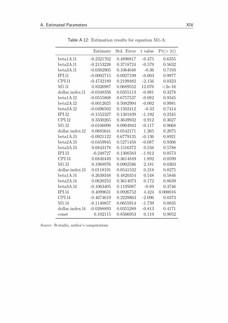
A. Estimated Parameters XIV
Table A.12: Estimation results for equation M1-A:
Estimate Std. Error t value Pr(> |t|)
beta1A.l1 -0.2321762 0.4890817 -0.475 0.6355beta2A.l1 -0.2153226 0.3718724 -0.579 0.5632beta3A.l1 -0.0382905 0.1064048 -0.36 0.7193IPI.l1 -0.0002715 0.0927199 -0.003 0.9977CPI.l1 -0.4742189 0.2199482 -2.156 0.0323M1.l1 0.8326987 0.0689552 12.076 <2e-16dollar.index.l1 -0.0348356 0.0355113 -0.981 0.3278beta1A.l2 -0.0555808 0.6757537 -0.082 0.9345beta2A.l2 -0.0012025 0.5082994 -0.002 0.9981beta3A.l2 -0.0496502 0.1502412 -0.33 0.7414IPI.l2 -0.1552327 0.1301839 -1.192 0.2345CPI.l2 0.3330265 0.3649932 0.912 0.3627M1.l2 -0.0106098 0.0904943 -0.117 0.9068dollar.index.l2 0.0685641 0.0542171 1.265 0.2075beta1A.l3 -0.0921122 0.6779135 -0.136 0.8921beta2A.l3 -0.0459945 0.5271458 -0.087 0.9306beta3A.l3 0.0843178 0.1516372 0.556 0.5788IPI.l3 -0.248727 0.1300583 -1.912 0.0573CPI.l3 0.6840449 0.3614849 1.892 0.0599M1.l3 0.1968976 0.0902586 2.181 0.0303dollar.index.l3 0.0118191 0.0541532 0.218 0.8275beta1A.l4 0.2639348 0.4820354 0.548 0.5846beta2A.l4 0.0620252 0.3614073 0.172 0.8639beta3A.l4 -0.1063405 0.1195087 -0.89 0.3746IPI.l4 0.4099631 0.0926752 4.424 0.000016CPI.l4 -0.4674619 0.2229863 -2.096 0.0373M1.l4 -0.1140857 0.0655914 -1.739 0.0835dollar.index.l4 -0.0288893 0.0355289 -0.813 0.4171const 0.102115 0.8566953 0.119 0.9052
Source: R-studio, author’s computations

A. Estimated Parameters XV
Table A.13: Estimation results for equation USDI-A:
Estimate Std. Error t value Pr(> |t|)
beta1A.l1 0.750963 1.019285 0.737 0.462143beta2A.l1 0.494768 0.775011 0.638 0.52395beta3A.l1 0.331411 0.221756 1.494 0.136641IPI.l1 -0.124842 0.193236 -0.646 0.518987CPI.l1 0.06406 0.458389 0.14 0.888999M1.l1 0.103181 0.143708 0.718 0.473609dollar.index.l1 1.267837 0.074008 17.131 <2e-16beta1A.l2 -1.227661 1.408324 -0.872 0.384418beta2A.l2 -0.69714 1.059336 -0.658 0.511244beta3A.l2 0.053637 0.313115 0.171 0.864161IPI.l2 -0.447531 0.271313 -1.649 0.100632CPI.l2 1.178531 0.760675 1.549 0.122901M1.l2 -0.090343 0.188597 -0.479 0.632448dollar.index.l2 -0.412151 0.112993 -3.648 0.000338beta1A.l3 0.788821 1.412825 0.558 0.577251beta2A.l3 0.600461 1.098614 0.547 0.585295beta3A.l3 -0.552163 0.316024 -1.747 0.08215IPI.l3 0.927752 0.271052 3.423 0.000753CPI.l3 -1.658987 0.753363 -2.202 0.028812M1.l3 0.076378 0.188106 0.406 0.685153dollar.index.l3 0.075684 0.11286 0.671 0.503253beta1A.l4 -0.511221 1.0046 -0.509 0.611403beta2A.l4 -0.48123 0.753201 -0.639 0.523618beta3A.l4 0.261161 0.249066 1.049 0.295658IPI.l4 -0.375264 0.193143 -1.943 0.053441CPI.l4 0.917627 0.464721 1.975 0.049706M1.l4 -0.097845 0.136698 -0.716 0.474973dollar.index.l4 0.004225 0.074045 0.057 0.954553const -0.088452 1.785421 -0.05 0.960538
Source: R-studio, author’s computations

A. Estimated Parameters XVI
NS-M-B
Figure A.5: NS-M-B estimation results - latent variables3
45
67
8
Diagram of fit and residuals for beta1B
0 50 100 150 200
−0.
50.
00.
5
0 2 4 6 8 10 12
0.0
0.8
Lag
ACF Residuals
2 4 6 8 10 12
−0.
10
Lag
PACF Residuals
−5
−3
−1
Diagram of fit and residuals for beta2B
0 50 100 150 200
−1.
00.
00.
50 2 4 6 8 10 12
0.0
0.8
Lag
ACF Residuals
2 4 6 8 10 12
−0.
10
Lag
PACF Residuals
−6
−2
02
4
Diagram of fit and residuals for beta3B
0 50 100 150 200
−2
−1
01
2
0 2 4 6 8 10 12
0.0
0.8
Lag
ACF Residuals
2 4 6 8 10 12
−0.
10
Lag
PACF Residuals
Source: author’s computations

A. Estimated Parameters XVII
Figure A.6: NS-M-B estimation results - macroeconomic variables
−15
−5
05
Diagram of fit and residuals for IPI
0 50 100 150 200
−4
−2
02
0 2 4 6 8 10 12
−0.
40.
8
Lag
ACF Residuals
2 4 6 8 10 12
−0.
40.
0
Lag
PACF Residuals
02
4
Diagram of fit and residuals for CPI
0 50 100 150 200
−1.
5−
0.5
0.5
0 2 4 6 8 10 12
−0.
51.
0
Lag
ACF Residuals
2 4 6 8 10 12
−0.
50.
1Lag
PACF Residuals
−5
05
1015
Diagram of fit and residuals for M1
0 50 100 150 200
−4
−2
02
4
0 2 4 6 8 10 12
−0.
20.
8
Lag
ACF Residuals
2 4 6 8 10 12
−0.
30.
1
Lag
PACF Residuals
−10
010
20
Diagram of fit and residuals for dollar.index
0 50 100 150 200
−4
02
46
0 2 4 6 8 10 12
−0.
40.
8
Lag
ACF Residuals
2 4 6 8 10 12
−0.
40.
1
Lag
PACF Residuals
Source: author’s computations

A. Estimated Parameters XVIII
Table A.14: Estimation results for equation beta1B:
Estimate Std. Error t value Pr(> |t|)
beta1B.l1 1.029331 0.113764 9.048 <2e-16beta2B.l1 0.027114 0.086544 0.313 0.7544beta3B.l1 0.037094 0.023762 1.561 0.1201IPI.l1 -0.006783 0.021261 -0.319 0.75CPI.l1 -0.040469 0.050465 -0.802 0.4236M1.l1 0.008559 0.015894 0.539 0.5908dollar.index.l1 -0.001695 0.008164 -0.208 0.8358beta1B.l2 -0.216342 0.15742 -1.374 0.1709beta2B.l2 0.074599 0.121353 0.615 0.5394beta3B.l2 -0.035845 0.032578 -1.1 0.2725IPI.l2 0.010134 0.029844 0.34 0.7346CPI.l2 0.037715 0.083768 0.45 0.653M1.l2 -0.027528 0.020852 -1.32 0.1883dollar.index.l2 0.002447 0.012464 0.196 0.8446beta1B.l3 0.272887 0.157818 1.729 0.0853beta2B.l3 -0.128221 0.125575 -1.021 0.3085beta3B.l3 -0.010733 0.032663 -0.329 0.7428IPI.l3 -0.026621 0.029824 -0.893 0.3732CPI.l3 -0.082999 0.083002 -1 0.3185M1.l3 0.006986 0.020795 0.336 0.7373dollar.index.l3 -0.008111 0.012437 -0.652 0.515beta1B.l4 -0.103879 0.111849 -0.929 0.3542beta2B.l4 0.045187 0.085987 0.526 0.5998beta3B.l4 0.004301 0.025946 0.166 0.8685IPI.l4 0.020133 0.021333 0.944 0.3465CPI.l4 0.044712 0.051191 0.873 0.3835M1.l4 0.009774 0.015122 0.646 0.5188dollar.index.l4 0.008737 0.008158 1.071 0.2855const 0.24222 0.202204 1.198 0.2324
Source: R-studio, author’s computations
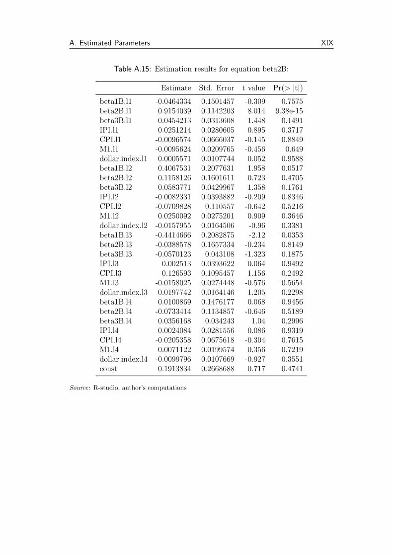
A. Estimated Parameters XIX
Table A.15: Estimation results for equation beta2B:
Estimate Std. Error t value Pr(> |t|)
beta1B.l1 -0.0464334 0.1501457 -0.309 0.7575beta2B.l1 0.9154039 0.1142203 8.014 9.38e-15beta3B.l1 0.0454213 0.0313608 1.448 0.1491IPI.l1 0.0251214 0.0280605 0.895 0.3717CPI.l1 -0.0096574 0.0666037 -0.145 0.8849M1.l1 -0.0095624 0.0209765 -0.456 0.649dollar.index.l1 0.0005571 0.0107744 0.052 0.9588beta1B.l2 0.4067531 0.2077631 1.958 0.0517beta2B.l2 0.1158126 0.1601611 0.723 0.4705beta3B.l2 0.0583771 0.0429967 1.358 0.1761IPI.l2 -0.0082331 0.0393882 -0.209 0.8346CPI.l2 -0.0709828 0.110557 -0.642 0.5216M1.l2 0.0250092 0.0275201 0.909 0.3646dollar.index.l2 -0.0157955 0.0164506 -0.96 0.3381beta1B.l3 -0.4414666 0.2082875 -2.12 0.0353beta2B.l3 -0.0388578 0.1657334 -0.234 0.8149beta3B.l3 -0.0570123 0.043108 -1.323 0.1875IPI.l3 0.002513 0.0393622 0.064 0.9492CPI.l3 0.126593 0.1095457 1.156 0.2492M1.l3 -0.0158025 0.0274448 -0.576 0.5654dollar.index.l3 0.0197742 0.0164146 1.205 0.2298beta1B.l4 0.0100869 0.1476177 0.068 0.9456beta2B.l4 -0.0733414 0.1134857 -0.646 0.5189beta3B.l4 0.0356168 0.034243 1.04 0.2996IPI.l4 0.0024084 0.0281556 0.086 0.9319CPI.l4 -0.0205358 0.0675618 -0.304 0.7615M1.l4 0.0071122 0.0199574 0.356 0.7219dollar.index.l4 -0.0099796 0.0107669 -0.927 0.3551const 0.1913834 0.2668688 0.717 0.4741
Source: R-studio, author’s computations
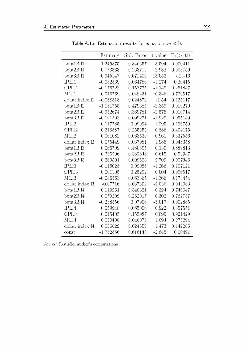
A. Estimated Parameters XX
Table A.16: Estimation results for equation beta3B:
Estimate Std. Error t value Pr(> |t|)
beta1B.l1 1.245875 0.346657 3.594 0.000411beta2B.l1 0.773333 0.263712 2.932 0.003759beta3B.l1 0.945147 0.072406 13.053 <2e-16IPI.l1 -0.082539 0.064786 -1.274 0.20415CPI.l1 -0.176723 0.153775 -1.149 0.251847M1.l1 -0.016769 0.048431 -0.346 0.729517dollar.index.l1 -0.038313 0.024876 -1.54 0.125117beta1B.l2 -1.131755 0.479685 -2.359 0.019279beta2B.l2 -0.952674 0.369781 -2.576 0.010714beta3B.l2 -0.191503 0.099271 -1.929 0.055149IPI.l2 0.117785 0.09094 1.295 0.196759CPI.l2 0.213387 0.255255 0.836 0.404175M1.l2 0.061082 0.063539 0.961 0.337556dollar.index.l2 0.075449 0.037981 1.986 0.048358beta1B.l3 0.066709 0.480895 0.139 0.889813beta2B.l3 0.235206 0.382646 0.615 0.53947beta3B.l3 0.269591 0.099528 2.709 0.007346IPI.l3 -0.115023 0.09088 -1.266 0.207121CPI.l3 0.001105 0.25292 0.004 0.996517M1.l3 -0.086563 0.063365 -1.366 0.173454dollar.index.l3 -0.07716 0.037898 -2.036 0.043083beta1B.l4 0.110261 0.340821 0.324 0.746647beta2B.l4 0.079209 0.262017 0.302 0.762737beta3B.l4 -0.238556 0.07906 -3.017 0.002885IPI.l4 0.059948 0.065006 0.922 0.357551CPI.l4 0.015405 0.155987 0.099 0.921429M1.l4 0.050408 0.046078 1.094 0.275294dollar.index.l4 0.036622 0.024859 1.473 0.142286const -1.752856 0.616148 -2.845 0.00491
Source: R-studio, author’s computations

A. Estimated Parameters XXI
Table A.17: Estimation results for equation IPI-B:
Estimate Std. Error t value Pr(> |t|)
beta1B.l1 -0.418929 0.385221 -1.088 0.27814beta2B.l1 -0.245557 0.293049 -0.838 0.40308beta3B.l1 0.101998 0.080461 1.268 0.2064IPI.l1 0.934568 0.071993 12.981 <2e-16CPI.l1 0.181627 0.170882 1.063 0.28913M1.l1 -0.008724 0.053818 -0.162 0.87139dollar.index.l1 0.038624 0.027643 1.397 0.16391beta1B.l2 1.016896 0.533047 1.908 0.05788beta2B.l2 0.726865 0.410917 1.769 0.07845beta3B.l2 0.08772 0.110314 0.795 0.42746IPI.l2 0.202305 0.101056 2.002 0.04666CPI.l2 -0.341713 0.28365 -1.205 0.22976M1.l2 -0.043193 0.070607 -0.612 0.54141dollar.index.l2 -0.093697 0.042206 -2.22 0.02756beta1B.l3 -0.492061 0.534393 -0.921 0.35828beta2B.l3 -0.158372 0.425214 -0.372 0.70995beta3B.l3 -0.110017 0.1106 -0.995 0.32108IPI.l3 0.024861 0.100989 0.246 0.80581CPI.l3 0.24652 0.281056 0.877 0.38148M1.l3 -0.017873 0.070414 -0.254 0.79989dollar.index.l3 0.004178 0.042114 0.099 0.92108beta1B.l4 -0.034646 0.378735 -0.091 0.92721beta2B.l4 -0.309361 0.291165 -1.062 0.28931beta3B.l4 -0.071587 0.087856 -0.815 0.41615IPI.l4 -0.210699 0.072237 -2.917 0.00395CPI.l4 -0.228186 0.17334 -1.316 0.18956M1.l4 0.081265 0.051204 1.587 0.11409dollar.index.l4 0.053347 0.027624 1.931 0.05489const 0.076933 0.684692 0.112 0.91065
Source: R-studio, author’s computations

A. Estimated Parameters XXII
Table A.18: Estimation results for equation CPI-B:
Estimate Std. Error t value Pr(> |t|)
beta1B.l1 0.160957 0.167895 0.959 0.33889beta2B.l1 -0.109462 0.127723 -0.857 0.39246beta3B.l1 -0.019793 0.035068 -0.564 0.57311IPI.l1 -0.005298 0.031378 -0.169 0.8661CPI.l1 1.285645 0.074477 17.262 <2e-16M1.l1 -0.01603 0.023456 -0.683 0.49514dollar.index.l1 -0.023339 0.012048 -1.937 0.05415beta1B.l2 -0.065198 0.232324 -0.281 0.77929beta2B.l2 0.239081 0.179095 1.335 0.18343beta3B.l2 0.049947 0.04808 1.039 0.30014IPI.l2 0.115645 0.044044 2.626 0.00932CPI.l2 -0.596178 0.123626 -4.822 0.00000282M1.l2 0.018982 0.030773 0.617 0.53806dollar.index.l2 0.013212 0.018395 0.718 0.47346beta1B.l3 0.113062 0.23291 0.485 0.62791beta2B.l3 0.06575 0.185326 0.355 0.72313beta3B.l3 0.002818 0.048204 0.058 0.95344IPI.l3 -0.109023 0.044015 -2.477 0.01409CPI.l3 0.173631 0.122496 1.417 0.15792M1.l3 0.006827 0.030689 0.222 0.82418dollar.index.l3 -0.021795 0.018355 -1.187 0.23649beta1B.l4 -0.20222 0.165068 -1.225 0.222beta2B.l4 -0.156037 0.126901 -1.23 0.22031beta3B.l4 -0.054729 0.038291 -1.429 0.1545IPI.l4 0.006337 0.031484 0.201 0.84068CPI.l4 0.035198 0.075549 0.466 0.6418M1.l4 -0.015076 0.022317 -0.676 0.50013dollar.index.l4 0.021144 0.01204 1.756 0.0806const 0.277749 0.298417 0.931 0.35312
Source: R-studio, author’s computations
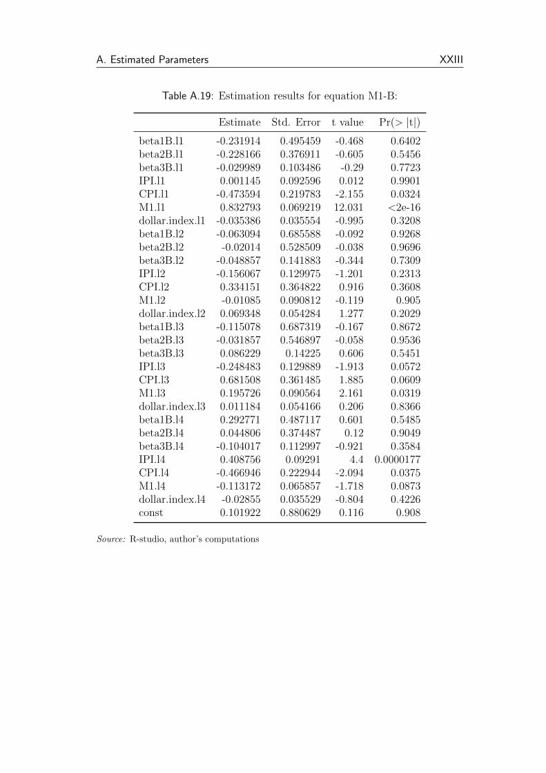
A. Estimated Parameters XXIII
Table A.19: Estimation results for equation M1-B:
Estimate Std. Error t value Pr(> |t|)
beta1B.l1 -0.231914 0.495459 -0.468 0.6402beta2B.l1 -0.228166 0.376911 -0.605 0.5456beta3B.l1 -0.029989 0.103486 -0.29 0.7723IPI.l1 0.001145 0.092596 0.012 0.9901CPI.l1 -0.473594 0.219783 -2.155 0.0324M1.l1 0.832793 0.069219 12.031 <2e-16dollar.index.l1 -0.035386 0.035554 -0.995 0.3208beta1B.l2 -0.063094 0.685588 -0.092 0.9268beta2B.l2 -0.02014 0.528509 -0.038 0.9696beta3B.l2 -0.048857 0.141883 -0.344 0.7309IPI.l2 -0.156067 0.129975 -1.201 0.2313CPI.l2 0.334151 0.364822 0.916 0.3608M1.l2 -0.01085 0.090812 -0.119 0.905dollar.index.l2 0.069348 0.054284 1.277 0.2029beta1B.l3 -0.115078 0.687319 -0.167 0.8672beta2B.l3 -0.031857 0.546897 -0.058 0.9536beta3B.l3 0.086229 0.14225 0.606 0.5451IPI.l3 -0.248483 0.129889 -1.913 0.0572CPI.l3 0.681508 0.361485 1.885 0.0609M1.l3 0.195726 0.090564 2.161 0.0319dollar.index.l3 0.011184 0.054166 0.206 0.8366beta1B.l4 0.292771 0.487117 0.601 0.5485beta2B.l4 0.044806 0.374487 0.12 0.9049beta3B.l4 -0.104017 0.112997 -0.921 0.3584IPI.l4 0.408756 0.09291 4.4 0.0000177CPI.l4 -0.466946 0.222944 -2.094 0.0375M1.l4 -0.113172 0.065857 -1.718 0.0873dollar.index.l4 -0.02855 0.035529 -0.804 0.4226const 0.101922 0.880629 0.116 0.908
Source: R-studio, author’s computations
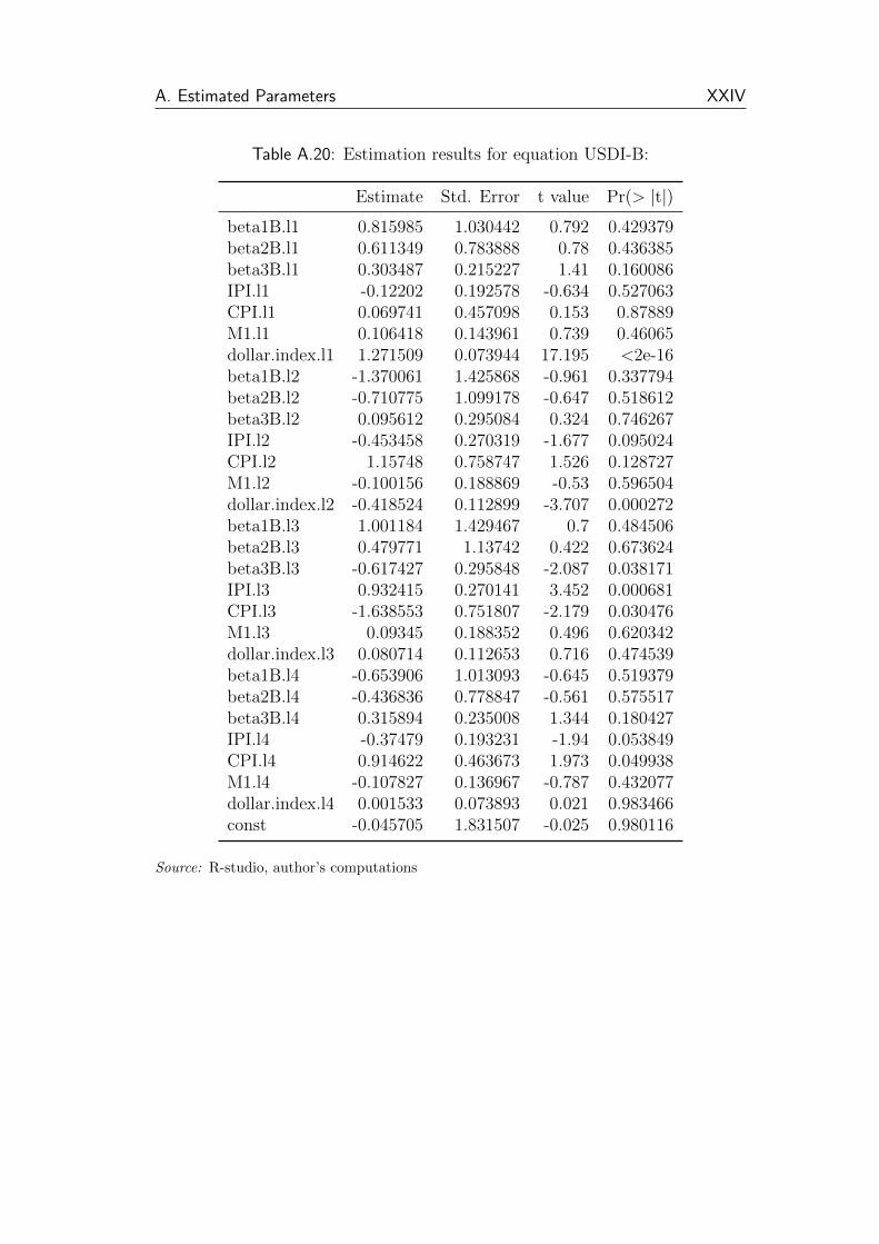
A. Estimated Parameters XXIV
Table A.20: Estimation results for equation USDI-B:
Estimate Std. Error t value Pr(> |t|)
beta1B.l1 0.815985 1.030442 0.792 0.429379beta2B.l1 0.611349 0.783888 0.78 0.436385beta3B.l1 0.303487 0.215227 1.41 0.160086IPI.l1 -0.12202 0.192578 -0.634 0.527063CPI.l1 0.069741 0.457098 0.153 0.87889M1.l1 0.106418 0.143961 0.739 0.46065dollar.index.l1 1.271509 0.073944 17.195 <2e-16beta1B.l2 -1.370061 1.425868 -0.961 0.337794beta2B.l2 -0.710775 1.099178 -0.647 0.518612beta3B.l2 0.095612 0.295084 0.324 0.746267IPI.l2 -0.453458 0.270319 -1.677 0.095024CPI.l2 1.15748 0.758747 1.526 0.128727M1.l2 -0.100156 0.188869 -0.53 0.596504dollar.index.l2 -0.418524 0.112899 -3.707 0.000272beta1B.l3 1.001184 1.429467 0.7 0.484506beta2B.l3 0.479771 1.13742 0.422 0.673624beta3B.l3 -0.617427 0.295848 -2.087 0.038171IPI.l3 0.932415 0.270141 3.452 0.000681CPI.l3 -1.638553 0.751807 -2.179 0.030476M1.l3 0.09345 0.188352 0.496 0.620342dollar.index.l3 0.080714 0.112653 0.716 0.474539beta1B.l4 -0.653906 1.013093 -0.645 0.519379beta2B.l4 -0.436836 0.778847 -0.561 0.575517beta3B.l4 0.315894 0.235008 1.344 0.180427IPI.l4 -0.37479 0.193231 -1.94 0.053849CPI.l4 0.914622 0.463673 1.973 0.049938M1.l4 -0.107827 0.136967 -0.787 0.432077dollar.index.l4 0.001533 0.073893 0.021 0.983466const -0.045705 1.831507 -0.025 0.980116
Source: R-studio, author’s computations
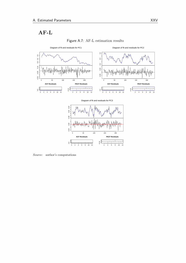
A. Estimated Parameters XXV
AF-L
Figure A.7: AF-L estimation results−
0.5
0.0
0.5
Diagram of fit and residuals for PC1
0 50 100 150 200−0.
20−
0.05
0.10
0 2 4 6 8 10 12
0.0
Lag
ACF Residuals
2 4 6 8 10 12
−0.
10
Lag
PACF Residuals
−0.
20.
00.
2
Diagram of fit and residuals for PC2
0 50 100 150 200
−0.
050.
05
0 2 4 6 8 10 12
0.0
Lag
ACF Residuals
2 4 6 8 10 12
−0.
10
Lag
PACF Residuals
−0.
060.
000.
04
Diagram of fit and residuals for PC3
0 50 100 150 200
−0.
040.
00
0 2 4 6 8 10 12
0.0
Lag
ACF Residuals
2 4 6 8 10 12
−0.
10
Lag
PACF Residuals
Source: author’s computations
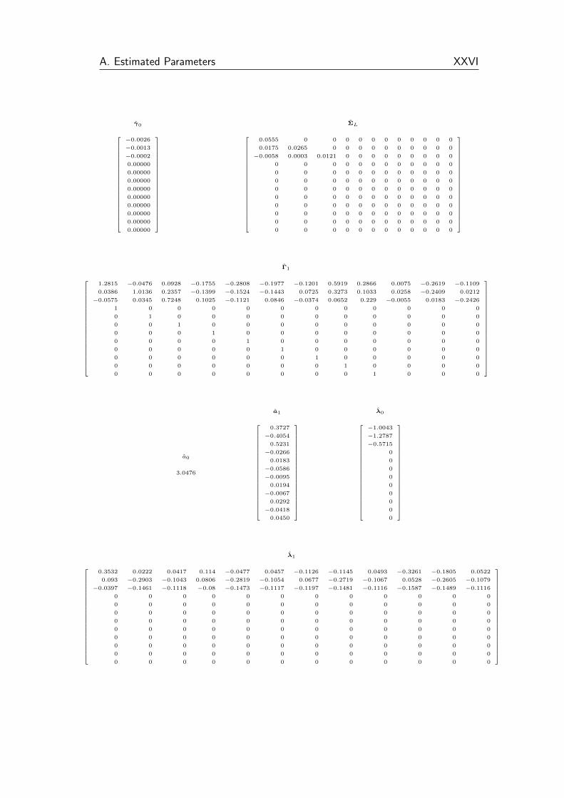
A. Estimated Parameters XXVI
γ0
−0.0026
−0.0013
−0.0002
0.00000
0.00000
0.00000
0.00000
0.00000
0.00000
0.00000
0.00000
0.00000
ΣL
0.0555 0 0 0 0 0 0 0 0 0 0 0
0.0175 0.0265 0 0 0 0 0 0 0 0 0 0
−0.0058 0.0003 0.0121 0 0 0 0 0 0 0 0 0
0 0 0 0 0 0 0 0 0 0 0 0
0 0 0 0 0 0 0 0 0 0 0 0
0 0 0 0 0 0 0 0 0 0 0 0
0 0 0 0 0 0 0 0 0 0 0 0
0 0 0 0 0 0 0 0 0 0 0 0
0 0 0 0 0 0 0 0 0 0 0 0
0 0 0 0 0 0 0 0 0 0 0 0
0 0 0 0 0 0 0 0 0 0 0 0
0 0 0 0 0 0 0 0 0 0 0 0
Γ1
1.2815 −0.0476 0.0928 −0.1755 −0.2808 −0.1977 −0.1201 0.5919 0.2866 0.0075 −0.2619 −0.1109
0.0386 1.0136 0.2357 −0.1399 −0.1524 −0.1443 0.0725 0.3273 0.1033 0.0258 −0.2409 0.0212
−0.0575 0.0345 0.7248 0.1025 −0.1121 0.0846 −0.0374 0.0652 0.229 −0.0055 0.0183 −0.2426
1 0 0 0 0 0 0 0 0 0 0 0
0 1 0 0 0 0 0 0 0 0 0 0
0 0 1 0 0 0 0 0 0 0 0 0
0 0 0 1 0 0 0 0 0 0 0 0
0 0 0 0 1 0 0 0 0 0 0 0
0 0 0 0 0 1 0 0 0 0 0 0
0 0 0 0 0 0 1 0 0 0 0 0
0 0 0 0 0 0 0 1 0 0 0 0
0 0 0 0 0 0 0 0 1 0 0 0
a0
3.0476
a1
0.3727
−0.4054
0.5231
−0.0266
0.0183
−0.0586
−0.0095
0.0194
−0.0067
0.0292
−0.0418
0.0450
λ0
−1.0043
−1.2787
−0.5715
0
0
0
0
0
0
0
0
0
λ1
0.3532 0.0222 0.0417 0.114 −0.0477 0.0457 −0.1126 −0.1145 0.0493 −0.3261 −0.1805 0.0522
0.093 −0.2903 −0.1043 0.0806 −0.2819 −0.1054 0.0677 −0.2719 −0.1067 0.0528 −0.2605 −0.1079
−0.0397 −0.1461 −0.1118 −0.08 −0.1473 −0.1117 −0.1197 −0.1481 −0.1116 −0.1587 −0.1489 −0.1116
0 0 0 0 0 0 0 0 0 0 0 0
0 0 0 0 0 0 0 0 0 0 0 0
0 0 0 0 0 0 0 0 0 0 0 0
0 0 0 0 0 0 0 0 0 0 0 0
0 0 0 0 0 0 0 0 0 0 0 0
0 0 0 0 0 0 0 0 0 0 0 0
0 0 0 0 0 0 0 0 0 0 0 0
0 0 0 0 0 0 0 0 0 0 0 0
0 0 0 0 0 0 0 0 0 0 0 0

A. Estimated Parameters XXVII
AF-M
ˆγ0
0.0085
0.0089
0.0043
0.4376
0.3108
0.0850
−1.6297
ΣM
0.0565 0.0000 0.0000 0.0000 0.0000 0.0000 0.0000
0.0186 0.0260 0.0000 0.0000 0.0000 0.0000 0.0000
−0.0060 0.0007 0.0125 0.0000 0.0000 0.0000 0.0000
0.0214 −0.1639 −0.0381 0.8929 0.0000 0.0000 0.0000
0.0205 0.0159 0.0263 −0.0054 0.4085 0.0000 0.0000
0.0453 −0.1196 −0.1882 −0.2425 −0.1423 1.0948 0.0000
0.0100 −0.1351 −0.1522 0.2242 −0.7809 −0.2006 2.2204
ˆΓ1
1.0145 0.0051 −0.2648 0.0015 −0.0092 0.0016 −0.0008
0.0010 0.9391 0.3156 −0.0015 −0.0022 −0.0002 0.0002
−0.0005 −0.0011 0.7958 0.0004 −0.0018 −0.0002 0.0000
0.3155 1.2358 −4.4190 0.9934 −0.2053 0.0159 −0.0304
0.1741 −0.2373 0.6042 0.0104 0.8529 0.0030 −0.0196
−1.2385 1.1659 3.8795 −0.0269 0.1638 0.9008 0.0386
−0.3722 −0.4108 −14.8225 −0.0179 0.6828 −0.0178 0.9598
ˆa0
0.2588
ˆa1
0.3650
−0.4117
0.5325
−0.0004
−0.0011
−0.0003
0.0001
ˆλ0
−0.2855
−0.2014
−0.1737
−0.1783
−0.1790
−0.3137
0.1828
ˆλ1
0.0854 −0.0048 −0.0045 0.0204 −0.1800 0.0081 −0.0063
−0.0007 0.0003 −0.0003 −0.0370 −0.0473 −0.0450 0.0082
−0.0069 0.0007 0.0000 −0.0278 −0.0269 −0.0187 0.0011
−0.0025 0.0006 −0.0002 −0.0075 −0.0313 0.0368 −0.0164
0.0110 −0.0011 −0.0007 −0.0013 0.0000 −0.0060 0.0056
0.0433 −0.0016 −0.0029 −0.0315 −0.2191 −0.0401 0.0045
−0.0234 0.0019 0.0012 −0.0210 0.0249 −0.0088 −0.0022
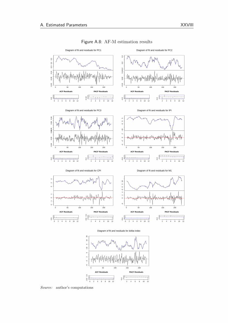
A. Estimated Parameters XXVIII
Figure A.8: AF-M estimation results
−0.
50.
00.
5Diagram of fit and residuals for PC1
0 50 100 150 200−0.
20−
0.05
0.10
0 2 4 6 8 10 12
0.0
Lag
ACF Residuals
2 4 6 8 10 12
−0.
10
Lag
PACF Residuals
−0.
20.
00.
2
Diagram of fit and residuals for PC2
0 50 100 150 200−0.
100.
000.
10
0 2 4 6 8 10 12
−0.
2
Lag
ACF Residuals
2 4 6 8 10 12
−0.
2
Lag
PACF Residuals
−0.
060.
000.
04
Diagram of fit and residuals for PC3
0 50 100 150 200−0.
040.
000.
04
0 2 4 6 8 10 12
−0.
2
Lag
ACF Residuals
2 4 6 8 10 12
−0.
2
Lag
PACF Residuals
−15
−5
05
Diagram of fit and residuals for IPI
0 50 100 150 200
−4
−2
02
0 2 4 6 8 10 12
−0.
4
Lag
ACF Residuals
2 4 6 8 10 12
−0.
4
Lag
PACF Residuals
02
4
Diagram of fit and residuals for CPI
0 50 100 150 200
−2
−1
01
0 2 4 6 8 10 12
−0.
5
Lag
ACF Residuals
2 4 6 8 10 12
−0.
60.
4
Lag
PACF Residuals
−5
05
10
Diagram of fit and residuals for M1
0 50 100 150 200
−4
02
4
0 2 4 6 8 10 12
−0.
4
Lag
ACF Residuals
2 4 6 8 10 12
−0.
4
Lag
PACF Residuals
−10
010
20
Diagram of fit and residuals for dollar.index
0 50 100 150 200
−6
−2
26
0 2 4 6 8 10 12
−0.
51.
0
Lag
ACF Residuals
2 4 6 8 10 12
−0.
4
Lag
PACF Residuals
Source: author’s computations
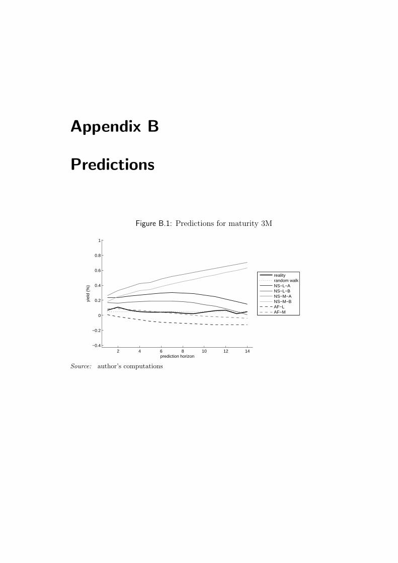
Appendix B
Predictions
Figure B.1: Predictions for maturity 3M
2 4 6 8 10 12 14−0.4
−0.2
0
0.2
0.4
0.6
0.8
1
prediction horizon
yiel
d (%
)
realityrandom walkNS−L−ANS−L−BNS−M−ANS−M−BAF−LAF−M
Source: author’s computations
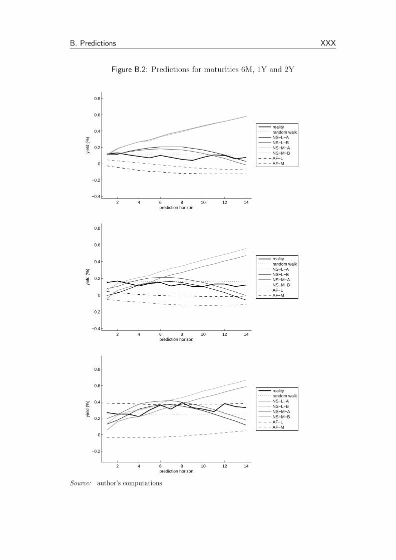
B. Predictions XXX
Figure B.2: Predictions for maturities 6M, 1Y and 2Y
2 4 6 8 10 12 14−0.4
−0.2
0
0.2
0.4
0.6
0.8
prediction horizon
yiel
d (%
)
realityrandom walkNS−L−ANS−L−BNS−M−ANS−M−BAF−LAF−M
2 4 6 8 10 12 14−0.4
−0.2
0
0.2
0.4
0.6
0.8
prediction horizon
yiel
d (%
)
realityrandom walkNS−L−ANS−L−BNS−M−ANS−M−BAF−LAF−M
2 4 6 8 10 12 14
−0.2
0
0.2
0.4
0.6
0.8
prediction horizon
yiel
d (%
)
realityrandom walkNS−L−ANS−L−BNS−M−ANS−M−BAF−LAF−M
Source: author’s computations

B. Predictions XXXI
Figure B.3: Predictions for maturities 3Y, 5Y and 7Y
2 4 6 8 10 12 14
0
0.2
0.4
0.6
0.8
1
prediction horizon
yiel
d (%
)
realityrandom walkNS−L−ANS−L−BNS−M−ANS−M−BAF−LAF−M
2 4 6 8 10 12 140.4
0.6
0.8
1
1.2
1.4
1.6
1.8
2
prediction horizon
yiel
d (%
)
realityrandom walkNS−L−ANS−L−BNS−M−ANS−M−BAF−LAF−M
2 4 6 8 10 12 14
1
1.2
1.4
1.6
1.8
2
2.2
2.4
2.6
prediction horizon
yiel
d (%
)
realityrandom walkNS−L−ANS−L−BNS−M−ANS−M−BAF−LAF−M
Source: author’s computations

B. Predictions XXXII
Figure B.4: Predictions for maturities 10Y, 20Y and 30Y
2 4 6 8 10 12 141.4
1.6
1.8
2
2.2
2.4
2.6
2.8
3
3.2
prediction horizon
yiel
d (%
)
realityrandom walkNS−L−ANS−L−BNS−M−ANS−M−BAF−LAF−M
2 4 6 8 10 12 14
2.5
3
3.5
4
4.5
prediction horizon
yiel
d (%
)
realityrandom walkNS−L−ANS−L−BNS−M−ANS−M−BAF−LAF−M
2 4 6 8 10 12 14
2.5
3
3.5
4
4.5
prediction horizon
yiel
d (%
)
realityrandom walkNS−L−ANS−L−BNS−M−ANS−M−BAF−LAF−M
Source: author’s computations