Une Approche Hybride de Simulation-Optimisation Basée sur ...

HAL Id: tel-00647353https://tel.archives-ouvertes.fr/tel-00647353

Submitted on 1 Dec 2011

HAL is a multi-disciplinary open accessarchive for the deposit and dissemination of sci-entific research documents, whether they are pub-lished or not. The documents may come fromteaching and research institutions in France orabroad, or from public or private research centers.

L’archive ouverte pluridisciplinaire HAL, estdestinée au dépôt et à la diffusion de documentsscientifiques de niveau recherche, publiés ou non,émanant des établissements d’enseignement et derecherche français ou étrangers, des laboratoirespublics ou privés.

Une Approche Hybride de Simulation-OptimisationBasée sur la fouille de Données pour les problèmes

d’ordonnancementAtif Shahzad

To cite this version:Atif Shahzad. Une Approche Hybride de Simulation-Optimisation Basée sur la fouille de Données pourles problèmes d’ordonnancement. Automatique / Robotique. Université de Nantes, 2011. Français.�tel-00647353�

https://tel.archives-ouvertes.fr/tel-00647353

https://hal.archives-ouvertes.fr

UNIVERSITÉ DE NANTES

École polytechnique de l’Université de Nantes

_____

ÉCOLE DOCTORALE

« SCIENCES ET TECHNOLOGIE DE L’INFORMATION ET MATHEMATIQUES »

Année 2011

Une Approche Hybride de Simulation-Optimisation

Basée sur la Fouille de Données pour les Problèmes d’ordonnancement

___________

THÈSE DE DOCTORAT Discipline : Génie Informatique

Spécialité : Automatique et Génie Informatique

Présentée et soutenue publiquement par

Muhammad Atif SHAHZAD Le 17 fév. 2011, devant le jury ci-dessous

Rapporteurs

Examinateurs

Henri PIERREVAL Professeur, IFMA, Clermont-Ferrand, France Jean-Charles BILLAUT Professeur, Université de Tours, France Abdelhakim ARTIBA Professeur, Université de Valenciennes, France Christos DIMOPOULOS Asst. Professor, Nicosia, Cyprus

Directeur de thèse : Pierre CASTAGNA Professeur, Université de Nantes, France Conencadrant : Nasser MEBARKI Maître de Conférences, Université de Nantes, France

ED : 503-119 (Uniquement pour STIM et SPIGA)

N° attribué par la bibliothèque

1 Acknowledgment

This dissertation would not have been possible without the guidance and the help of

several individuals who in one way or the other contributed and extended their valuable

assistance in the preparation and completion of this work.

I would like to thank Professor Henri PIERREVAL and Professor Jean-Charles BILLAUT

for accepting my request to examine this thesis as the official referees. I am also thankful

to Professor Abdelhakem ARTIBA and Associate Professor Christos DIMOPOULOS for

accepting the invitation to attend my thesis defense. I highly appreciate them all for

sparing some time and being flexible in the dates despite their busy schedules.

My utmost gratitude to my advisor Professor Pierre CASTAGNA, for his steadfast en-

couragement, kind concern and consideration during this work.

I would like to express the deepest appreciation to my thesis co-advisor,

Dr. Nasser MEBARKI who continually and convincingly conveyed a spirit of research. His

wide knowledge and logical way of thinking has been a great value for me. He provided

me with an untiring help, valuables suggestions and detailed and constructive insightful

comments throughout this work. Thank you very much for patiently correcting and edi-

ting my manuscript as well. Without his guidance and persistent help this dissertation

would have not been possible.

I greatly admire the persistent and meticulous attitude of Professor Jean-Jacque Loiseau,

incharge of the research team ACSED (Analyse et Commande des Systemes a Evenen-

ments Discrets). I wish to extend my warmest thanks to all members of the team for their

support and encouragement. In particular, I would like to thank Dr. Guillaume Pinot and

Dr. Olivier Boutin for offering their advice and suggestions whenever I needed them.

I would like to thank all the staff members at the IRCCyN for all their help, technical

and moral support.

2

Special thanks goes to Mme Somia ASHRAF, who encouraged me a lot to initiate this

work in France. Furthermore, I am greatly thankful to Miss Qudsia and Miss Brigette at

Alliance Francaise, Islamabad.

Where would I be without my family? My deepest gratitude goes to my family for their

unflagging love and support throughout my life; this dissertation is simply impossible

without them. I am greatly indebted to my father for his great care and attention, sparing

no effort to provide the best possible environment for me to grow up and showing me the

joy of intellectual pursuit ever since I was a child. Although he is no longer with us, he

is forever remembered. I have no suitable words to describe the everlasting love of my

mother. Her continuous support and unconditional love has been my greatest strength.

Despite all the hardships in the life, she provided with best possible environment and

the freedom to pursue my work thousands miles away. I am indebted to very loving and

kind support of my parents-in law as well. I owe loving thanks to my wife Aeysha and

my son Basim. Their support has been unconditional all these years; they have given up

many things for me to be at work; they have cherished with me every great moment,

supported me whenever I needed it and accompanying me through thick and thin. My

special gratitude to my brothers, my sisters and their families for their love and support.

Without their encouragement and support, it would have been impossible for me to finish

this work.

In my daily life, I have been blessed with a friendly and cheerful group of fellows. Thanks

are due to my friends, who have made each day of my stay in the city of Nantes, a new

experience for me. I treasured all precious moments we shared and would really like to

thank them all. Thanks to Raza for helping me (but not limited to this) to get on the road

to LATEX and provided an experienced ear for my doubts about working on thesis report.

Thanks to Kamran, for his fascinating discussions on the problems from whatever field

and to Quaid and Bilal for their witty presence and for the laughter and fun experiences we

have shared. Special thanks to Jamil Ahmed, Hassan Ijaz, Aamir Shehzad, Irfan Khokhar,

Amer Rasheed and their families for their company and continuous support. I am very

thankful to Sami ur-Rehman, Yasir Alam for being a great company and invaluable help

at many occasions. Thanks to everybody that has been a part of my life but I failed to

mention, thank you very much. There won’t be enough space if I’ll mention you all.

The financial support of the HEC (Higher Education Commission), Islamabad is grate-

fully acknowledged as well as Societe francaise d’exportation des ressources educatives

(SFERE) for providing administrative support.

Last but not the least, thanks to Almighty Allah for bestowing upon me the courage to

face the complexities of life and complete this project successfully.

�

1 Table of Contents

Introduction 3

1 Scheduling: A General Introduction 9

1.1 Introduction . . . . . . . . . . . . . . . . . . . . . . . . . . . . . . . . . . . 10

1.2 Elements of a Scheduling Problem . . . . . . . . . . . . . . . . . . . . . . . 11

1.3 Classes of Schedules . . . . . . . . . . . . . . . . . . . . . . . . . . . . . . . 18

1.4 Classification and Notations of Scheduling Problem . . . . . . . . . . . . . 22

1.5 Scheduling Phases . . . . . . . . . . . . . . . . . . . . . . . . . . . . . . . . 27

1.6 Job Shop Scheduling Problem . . . . . . . . . . . . . . . . . . . . . . . . . 27

1.7 Solving Methods . . . . . . . . . . . . . . . . . . . . . . . . . . . . . . . . 29

1.8 Conclusions . . . . . . . . . . . . . . . . . . . . . . . . . . . . . . . . . . . 32

2 A State of the Art Survey of Priority Dispatching Rules 33

2.1 Introduction . . . . . . . . . . . . . . . . . . . . . . . . . . . . . . . . . . . 33

2.2 Classification of Priority Dispatching Rules . . . . . . . . . . . . . . . . . . 35

2.3 Literature Reviews on Priority Dispatching Rules . . . . . . . . . . . . . . 38

2.4 Priority Dispatching Rules . . . . . . . . . . . . . . . . . . . . . . . . . . . 41

2.5 Comparative Studies and Important Factors . . . . . . . . . . . . . . . . . 48

2.6 Factors Affecting Performance of PDRs . . . . . . . . . . . . . . . . . . . . 50

2.7 Conclusions . . . . . . . . . . . . . . . . . . . . . . . . . . . . . . . . . . . 52

3 Correlation Among Tardiness Based Measures For PDRs 55

3.1 Introduction . . . . . . . . . . . . . . . . . . . . . . . . . . . . . . . . . . . 56

3.2 Tardiness Based Measures . . . . . . . . . . . . . . . . . . . . . . . . . . . 56

3.3 Experiments . . . . . . . . . . . . . . . . . . . . . . . . . . . . . . . . . . . 58

3.4 Results . . . . . . . . . . . . . . . . . . . . . . . . . . . . . . . . . . . . . . 60

3.5 Conclusions . . . . . . . . . . . . . . . . . . . . . . . . . . . . . . . . . . . 72

4 Learning based Approach in Scheduling: A Review 73

4.1 Introduction . . . . . . . . . . . . . . . . . . . . . . . . . . . . . . . . . . . 73

4.2 A General Overview of Literature on Learning Based Scheduling . . . . . . 74

4.3 Literature Review on Inductive Learning in Scheduling . . . . . . . . . . . 75

4.4 Parameters Influencing the Induction Algorithm . . . . . . . . . . . . . . 80

4.5 Conclusions . . . . . . . . . . . . . . . . . . . . . . . . . . . . . . . . . . . 81

5 Discovering Dispatching Rules For JSSP through Data Mining 85

5.1 Introduction . . . . . . . . . . . . . . . . . . . . . . . . . . . . . . . . . . . 86

5.2 Background . . . . . . . . . . . . . . . . . . . . . . . . . . . . . . . . . . . 86

5.3 Proposed Approach . . . . . . . . . . . . . . . . . . . . . . . . . . . . . . . 88

5.4 Experiments . . . . . . . . . . . . . . . . . . . . . . . . . . . . . . . . . . . 98

5.5 Results and Discussion . . . . . . . . . . . . . . . . . . . . . . . . . . . . . 100

5.6 Conclusions . . . . . . . . . . . . . . . . . . . . . . . . . . . . . . . . . . . 108

General Conclusions 111

A Priority Dispatching Rules 113

References 115

1 List of Figures

1.1 Temporal constraint: Absolute position and size of execution window . . . 12

1.2 Schedules for problem in Table 1.2 illustrating performance measures . . . 16

1.3 A bi-objective space with dominated and non-dominated solutions . . . . . 18

1.4 Classes of Schedules . . . . . . . . . . . . . . . . . . . . . . . . . . . . . . . 20

1.5 Schedules of the problem described in Table 1.3 . . . . . . . . . . . . . . . 21

1.6 A three machine flow shop, F3 . . . . . . . . . . . . . . . . . . . . . . . . 23

1.7 A three machine permutation flow shop,F3|prmu|− . . . . . . . . . . . . . 24

1.8 A three machine job shop, J3 . . . . . . . . . . . . . . . . . . . . . . . . . 24

1.9 Gantt diagram for a schedule for the problem in Table 1.7. . . . . . . . . . 29

1.10 Disjunctive graph representation of problem in Table 1.7 . . . . . . . . . . 29

1.11 Simplified Disjunctive graph representation of problem in Table 1.7 . . . . 30

1.12 Disjunctive graph representation of solution . . . . . . . . . . . . . . . . . 30

2.1 Classification Matrix of PDRs, adapted from (Kemppainen, 2005) . . . . . 39

3.1 Box plot of Tmax with (τ,η) = (7.5,90%) . . . . . . . . . . . . . . . . . . . . 61

3.2 Box plot of Tmax with (τ,η) = (12.5,90%) . . . . . . . . . . . . . . . . . . . 62

3.3 Box plot of Tmax with (τ,η) = (15,90%) . . . . . . . . . . . . . . . . . . . . 63

3.4 Box plot of Tmax with (τ,η) = (5,80%) . . . . . . . . . . . . . . . . . . . . . 64

3.5 Box plot of Tmax with (τ,η) = (7.5,80%) . . . . . . . . . . . . . . . . . . . . 64

3.6 Box plot of Tmax with (τ,η) = (8.75,80%) . . . . . . . . . . . . . . . . . . . 65

3.7 Tardiness distribution for rules of set 1 with corresponding (τ,η) . . . . . . 66

3.8 Tardiness distribution for rules of set 2 with corresponding (τ,η) . . . . . . 67

3.9 Comparison of Tmax and Trms for rules of set 1 . . . . . . . . . . . . . . . . 68

3.10 Comparison of Tmax and Trms for rules of set 2 . . . . . . . . . . . . . . . . 69

3.11 Comparison of Tmax and Trms for other rules . . . . . . . . . . . . . . . . . 70

5.1 The proposed framework . . . . . . . . . . . . . . . . . . . . . . . . . . . . 90

5.2 Simulation Module . . . . . . . . . . . . . . . . . . . . . . . . . . . . . . . 91

5.3 An Example of Generating Decision Tree from a Simple Training Block . . 93

5.4 Disjunctive Graph Solution Given by Tabu Search . . . . . . . . . . . . . . 96

5.5 Disjunctive Graph Solution Given by Rule Set . . . . . . . . . . . . . . . . 97

5.6 Standard Deviation based Discretization of for Lmax . . . . . . . . . . . 100

5.7 System Performance for T . . . . . . . . . . . . . . . . . . . . . . . . . . . 104

5.8 Box Plot of T for Test Instances . . . . . . . . . . . . . . . . . . . . . . . . 105

5.9 System Performance for Tmax . . . . . . . . . . . . . . . . . . . . . . . . . 106

5.10 Box Plot of Tmax for Test Instances . . . . . . . . . . . . . . . . . . . . . . 107

1 List of Tables

1.1 Some Performance Measures . . . . . . . . . . . . . . . . . . . . . . . . . . 15

1.2 An example problem to illustrate Regular measure . . . . . . . . . . . . . . 16

1.3 An example problem to illustrate classes of schedules . . . . . . . . . . . . 20

1.4 Some examples for the field α . . . . . . . . . . . . . . . . . . . . . . . . . 23

1.5 Some examples for the field β . . . . . . . . . . . . . . . . . . . . . . . . . 26

1.6a Some examples for the field γ . . . . . . . . . . . . . . . . . . . . . . . . . 26

1.6b Some MO examples for the field γ . . . . . . . . . . . . . . . . . . . . . . 27

1.7 An instance of a JSSP . . . . . . . . . . . . . . . . . . . . . . . . . . . . . 28

2.1 Relevant Literature Review on PDRs . . . . . . . . . . . . . . . . . . . . . 40

3.1 Simulation model parameters . . . . . . . . . . . . . . . . . . . . . . . . . 59

3.2 Operating conditions tested. . . . . . . . . . . . . . . . . . . . . . . . . . . 60

3.3 Confidence Interval for Correlation between Tmax and Trms . . . . . . . . . 71

4.1 Review of Literature . . . . . . . . . . . . . . . . . . . . . . . . . . . . . . 83

5.1 An Instance from the Test Data Set . . . . . . . . . . . . . . . . . . . . . . 96

5.2 Experimental Setup . . . . . . . . . . . . . . . . . . . . . . . . . . . . . . . 98

5.3 Selected Attributes for Tmax . . . . . . . . . . . . . . . . . . . . . . . . . . 99

5.4 A partial list of inferred rules for T . . . . . . . . . . . . . . . . . . . . . . 101

5.5 A partial list of inferred rules for Tmax . . . . . . . . . . . . . . . . . . . . 102

A.1 Priority Dispatching Rules . . . . . . . . . . . . . . . . . . . . . . . . . . . 113

1

GLOSSARY OF NOTATION

Sets

M Set of resources

J Set of jobs

O Set of operations

Oj Set of operations of jth job

♯ Cardinality of a set

f Set of Objectives

C Set of Constraints

Jj jth job

Mk kth machine

Ojk An operation of jth job to be processed on kth machine

Oj(i) ith operation of job Jj

Indices

j Index for job, jth job

k Index for machine, kthmachine

i Index for operation, ith operation of a given job

j,j Indexes for jobs

u,v Indexes for operations

Job Attributes

rj Ready time, Ready time of jth job

sj Start time of jth job

pj Total processing time of jth job

dj Due date of jth job.

dj Dead-line of jth job

Cj Completion time of jth job

oj Total number of operations of jth job.

Lj Lateness of jth job

Tj Tardiness of jth job

j Remaining processing time of jth job

ςj Slack of jth job

Wj Expected waiting time for jth job

�

2

Operation Attributes

pj(i) Processing time of ith operation of jth job

dj(i) Due date of ith operation of jth job

sj(i) Service start time of ith operation of jth job

Cj(i) Completion time of ith operation of jth job

pjk Processing time of an operation of jth job to be processed

on kth machine

djk Due date of an operation of jth job to be processed on

kth machine

sj(i) Service start time of an operation of jth job to be pro-

cessed on kth machine

Cjk Completion time of an operation of jth job to be proces-

sed on kth machine

Wj(i) Expected waiting time for ith operation of jth job

System parameters/Variables

t Current time

π A processing sequence

σ A schedule

τ Due-date tightness factor

ρ Due-date range

m Number of machines

n Number of jobs

nt Number of jobs in system at time t

µx Mean of x

E(x) Expectation of x

V ar(x) Variance of x

(x)+ max(x,0)

X set of input features.

�

1 Introduction

Over the last fifty years, scheduling theory has evolved as a major active area of research

attracting a wide spectrum of researchers ranging from computer and management scien-

tists to production engineers. There exist a significant amount of literature on a wide

variety of methods to solve different scheduling problems. These methods range from

industry-standard dispatching rules to state-of-the-art meta-heuristics and sophisticated

optimization algorithms.

Scheduling is concerned with solving a Constraint Optimization Problem (an optimization

problem with finite solution space for each of its instance (Colorni et al., 1996)).

The job shop problem is considered as one of the most general and well developed schedu-

ling problems with much practical significance. The problem is generally NP-hard (Non-

deterministic Polynomial-time hard) except for a very few special cases. Conway et al.

(1967) describes the problem as a fascinating challenge that is extremely hard to solve

despite its quite simple structure. The reason for computational intractability of job shop

scheduling problem is mainly its combinatorial nature besides many conflicting factors

that must be taken into account (Zobolas et al., 2008).

The history of solving job shop scheduling problem encompasses a wide spectrum of

approaches. Initially, the focus of researchers remained on the exact approaches. These

include the earlier efficient methods, mathematical methods and enumerative techniques.

Branch and bound are considered among the most successful exact methods, however

they demand phenomenal computing time to obtain an optimal solution (Zobolas et al.,

2008). Later on, an era of heuristic methodologies is observed, although simple dispatching

rules were already in use. Various bottleneck-based heuristics are developed during this

period. Thereafter, with the emergence of more sophisticated meta-heuristics and tech-

4 Introduction

niques based on artificial intelligence, substantial progress is made in late 80s and early 90s

(Jain and Meeran, 1998). Powerful meta-heuristics coupled with the computational power

of modern computer systems enabled to make use of these approaches on relatively larger

problems. However, Lawrence and Sewell (1997) found that the performance of these so-

lution methodologies deteriorates due to processing time uncertainty when compared to

dynamically updated heuristic schedules.

In dynamic scheduling, jobs are continually revealed during the process of schedule exe-

cution. Dynamic scheduling is closely related to real-time control, as decisions are to be

made based on the current state of the system. This on-line aspect greatly influences the

scheduling decisions as the schedule creation and schedule execution no longer remain two

different processes. Scheduling decisions are to be made in a very short time as the time

required to generate a schedule becomes relatively more important factor than merely

finding a best quality schedule in an extended period of time. Moreover, schedule is requi-

red to be highly reactive to cope with unanticipated circumstances. Priority dispatching

rules are considered as the best choice in such an environment mainly due to their ease

of implementation and intuitive appeal despite their poor performance in most of the

scheduling problems.

The priority dispatching rules based approach is the simplest and most used approach in

practice for dispatching jobs in real-time for processing on machines. Numerous studies

have been made on the nature, effectiveness and performance of different priority dis-

patching rules under varying scheduling conditions. Panwalker and Iskander (1977) has

reviewed 113 priority dispatching rules while new rules are continuously emerging. Howe-

ver, there is still a lack of satisfactory results in literature on the performance of priority

dispatching rules that would have lead to extensive real-world applications. Unfortunately,

the superiority of one scheduling rule to the other is not obvious and often conflicting re-

sults have been reported possibly due to different conditions and parameter-settings used

for the scheduling environment. Moreover, the performance of priority dispatching rules

is dependent on the performance criterion. An apparently highly efficient rule in regards

with one performance criteria may give very poor results for some other performance crite-

rion even under the same conditions. Even for the pragmatic priority scheduling approach,

the overall performance of priority dispatching rules diminishes due to the dynamic and

stochastic nature of the system.

Under the general title of Artificial Intelligence (AI), a series of new techniques emerged

in early 80s to solve the job shop scheduling problem (Jones and Rabelo, 1998). They in-

clude expert/knowledge-based systems, artificial neural networks and inductive learning.

These techniques generally employ both the quantitative and qualitative knowledge spe-

�

5

cific to problem domain as well as procedural knowledge of the solving methods. These

approaches are assumed to capture complex relationships and transform them into elegant

data structures for subsequent generation of heuristics. The heuristics obtained however,

are quite complex in most of the cases, as compared to priority dispatching rules. Moreo-

ver, systems based on these techniques are too time-consuming to build and quite complex

to maintain.

Knowledge acquisition is the basic step in developing the knowledge-base. The knowledge

source is usually a human expert, the simulation data or the historical data. A machine

learning technique employs this data as a set of training examples. These training examples

are used to train the machine-learning algorithm to acquire knowledge about the manufac-

turing system (Michalski et al., 1986, 1998). Intelligent decisions are then made (such as

selecting the best rule for each possible system state) in real time, based on this knowledge

(Nakasuka and Yoshida, 1992; Shaw et al., 1992; Yeong-Dae, 1994; Min and Yih, 2003).

The major drawbacks of priority dispatching rules include their performance-dependence

on the state of the system and non-existence of any single rule, superior to all the others

for all possible states the system might be in (Geiger et al., 2006). Meta-heuristics (e.g.

simulated annealing and tabu search) have an advantage over the priority dispatching

rules in terms of solution quality and robustness, however these are usually more difficult

to implement and tune, and computationally too complex to be used in a real time system.

Robust and better-quality solutions provided by meta-heuristics contain useful knowledge

about the problem domain and solution space explored. Such a set of solutions represents

a wealth of scheduling knowledge to the domain that can be transformed in a form of

decision tree or a rule-set. In this work, we propose an approach to exploit this scheduling

knowledge.

The proposed data mining-based approach discovers previously unknown dispatching rules

for job shop scheduling problem. An efficient meta-heuristic such as tabu search can

provide robust and better-quality solutions for a job shop scheduling problem that contains

useful knowledge about the problem domain and solution space explored. A set of such

solutions for different instances of a job shop scheduling problem represents a wealth of

scheduling knowledge to the domain. The idea is to exploit this scheduling knowledge and

to transform it in a form of decision tree or a rule-set. The rule-set may then be used as

a standard dispatching rule at the waiting lines of a job shop in an on-line manner.

�

6 Introduction

Thesis Organization

This thesis report is composed of five chapters. The first chapter presents the scheduling

problem and the basic concepts in the field of scheduling. The key elements, of which of

shop scheduling problem is composed as well as the notations used to characterize the

problem are recalled. Thereafter, we present different classes of schedules. Classification of

scheduling problems are then presented in order to distinguish different combinations of

scheduling environments, conditions and objectives. This follows with a formal definition

of job shop scheduling problem. Then the schedule visualization by Gantt diagram and

the scheduling problem representation using disjunctive graph formulation is described.

Finally, a general introduction to different methods used in solving job shop scheduling

problems are discussed.

The second chapter provides a state-of-the-art review on priority dispatching rules in

context with job shop scheduling environment. Frequently used classification schemes for

these pdrs found in literature are reviewed. This follows with a detailed discussion on the

structure and characteristics of most frequently used pdrs in literature.

In the third chapter, a simulation based analysis of tardiness based performance measures

for a set of frequently used pdrs is made in order to highlight the similarities/dissimilarities

in the behavior of pdrs. Tardiness based performance measures focus on different aspects

of a very important class of objectives in a manufacturing system. The first part of the

chapter presents these different tardiness based performance measures. These performance

measures are not independent of each other. Moreover, the relation among these perfor-

mance measures is generally not obvious even for simple scheduling strategies such as

priority dispatching rules. Based upon the behavior of different priority dispatching rules

in regards with these performance measures, we identify two sets of pdrs using the distri-

bution of the maximum tardiness (i.e. Tmax), a very important measure representing the

worst case behavior. The worst-case behavior in regards with tardiness is very difficult to

identify due to its value at a single-point only. However, it is possible to establish some

guidelines in predicting this worst-case behavior in regards with tardiness as well as the

width of the tardiness by evaluating root mean square tardiness (Trms). Results showing

the correlation among two very important measures, maximum tardiness (Tmax) and root

mean square tardiness (Trms) are presented along-with discussion on these results.

In chapter 4, a state-of-the-art survey on the application of learning based approaches

in the field of job shop scheduling is given. It provides an effective overview of the chal-

lenges and benefits related to the application of learning algorithms in solving scheduling

problems. The survey reveals that their is a lack of systematic use of the scheduling know-

�

7

ledge despite the fact that the approach has been acknowledged by most of the authors

as promising in scheduling domain. Moreover, it is generally not obvious how much a

certain set of scheduling data is relevant to the scheduling environment for desired ob-

jectives. The emergence of data mining has invoked the academic interest in analyzing

the complex problems like this in a more methodical way. A brief review of the factors

affecting the performance of inductive learning algorithm, for example feature selection

and discretization is given in the last part.

A data mining based approach to discover previously unknown priority dispatching rules

for job shop scheduling problem is presented in chapter 5. In the beginning, a brief des-

cription of some necessary background areas such as tabu search and data mining is given.

Then the proposed framework is presented along with the structure and functional de-

tails of the different modules. The approach is based upon seeking the knowledge that is

assumed to be embedded in the efficient solutions provided by the optimization module,

built using tabu search. The objective is to discover the scheduling concepts using data

mining and hence to obtain a set of rules capable of approximating the efficient solutions

for a job shop scheduling problem (JSSP). The data mining based scheduling framework

is implemented for a job shop problem with mean tardiness and maximum lateness as

the scheduling objectives. The results indicate the superior performance of the proposed

system relative to a number of priority dispatching rules and hence proves to be promising

approach.

�

1 Scheduling: A General

Introduction

1.1 Introduction . . . . . . . . . . . . . . . . . . . . . . . . . . . . 10

1.2 Elements of a Scheduling Problem . . . . . . . . . . . . . . . . 11

1.2.1 Jobs . . . . . . . . . . . . . . . . . . . . . . . . . . . . . . . . . . . . . . 11

1.2.2 Resources . . . . . . . . . . . . . . . . . . . . . . . . . . . . . . . . . . . 11

1.2.3 Constraints . . . . . . . . . . . . . . . . . . . . . . . . . . . . . . . . . . 12

1.2.4 Objectives . . . . . . . . . . . . . . . . . . . . . . . . . . . . . . . . . . . 13

1.3 Classes of Schedules . . . . . . . . . . . . . . . . . . . . . . . . 18

1.3.1 Feasible schedule . . . . . . . . . . . . . . . . . . . . . . . . . . . . . . . 19

1.3.2 Semi-active schedule . . . . . . . . . . . . . . . . . . . . . . . . . . . . . 19

1.3.3 Active schedule . . . . . . . . . . . . . . . . . . . . . . . . . . . . . . . . 19

1.3.4 Non-delay schedule . . . . . . . . . . . . . . . . . . . . . . . . . . . . . . 20

1.3.5 Optimal schedule . . . . . . . . . . . . . . . . . . . . . . . . . . . . . . . 20

1.4 Classification and Notations of Scheduling Problem . . . . . . . 22

1.4.1 α field: . . . . . . . . . . . . . . . . . . . . . . . . . . . . . . . . . . . . . 22

1.4.2 β field: . . . . . . . . . . . . . . . . . . . . . . . . . . . . . . . . . . . . . 25

1.4.3 γ field: . . . . . . . . . . . . . . . . . . . . . . . . . . . . . . . . . . . . . 25

1.5 Scheduling Phases . . . . . . . . . . . . . . . . . . . . . . . . . 27

1.5.1 Predictive Phase . . . . . . . . . . . . . . . . . . . . . . . . . . . . . . . 27

1.5.2 Reactive Phase . . . . . . . . . . . . . . . . . . . . . . . . . . . . . . . . 27

1.6 Job Shop Scheduling Problem . . . . . . . . . . . . . . . . . . . 27

1.6.1 Formal definition of JSSP . . . . . . . . . . . . . . . . . . . . . . . . . . 28

1.6.2 Graphical Representation . . . . . . . . . . . . . . . . . . . . . . . . . . 28

1.7 Solving Methods . . . . . . . . . . . . . . . . . . . . . . . . . . 29

1.7.1 Exact methods . . . . . . . . . . . . . . . . . . . . . . . . . . . . . . . . 30

1.7.2 Approximation methods . . . . . . . . . . . . . . . . . . . . . . . . . . . 30

1.8 Conclusions . . . . . . . . . . . . . . . . . . . . . . . . . . . . . 32

This chapter presents an overview of the scheduling domain and related concepts. The

key elements of shop scheduling problem and notations are presented. Different shop

scheduling environments along with classification of shop scheduling problems is given. A

10 Chapter 1. Scheduling: A General Introduction

formal definition of job shop scheduling problem (JSSP) and its representation are given.

Then a general introduction to different approaches used in solving JSSP are discussed.

1.1 Introduction

Scheduling is a decision-making process that is extensively encountered in a large variety

of systems. However it is widely used in manufacturing systems where it is generally

referred as machine scheduling. Machine scheduling is one of the most important issues in

the planning and operation of manufacturing systems. It is aimed at efficiently allocating

the available machines to jobs, or operations within jobs and subsequent time-phasing of

these jobs on individual machines (Shaw et al., 1992).

A solution to a scheduling problem represents a schedule (σ) that satisfies all the

constraints of the problem. A schedule is composed of following three major processes:

assignment : It is a process of allocating a machine to each task to be executed.

sequencing : It is the process of assigning an order of execution of the tasks on each

machine.

timetabling : It is the process of assigning a start time and finish time to each task.

However, these three processes may be dealt as separate problems, known as assignment

problem, sequencing problem and timetabling problem respectively (French, 1982).

Scheduling problems are generally very complex in nature due to their combinatorial na-

ture. However these problems are extensively studied in literature as benchmark problems

for the optimization methods apart from their own practical applications. Traditional ap-

proaches to solve scheduling problems use simulation, analytical models, heuristics or

combination of these methods.

Different components of a scheduling problem are the tasks, constraints, resources and

the objective functions. In the following, these key elements of a scheduling problem are

presented.

�

1.2 Elements of a Scheduling Problem 11

1.2 Elements of a Scheduling Problem

A scheduling problem is a typical representative of a combinatorial optimization class of

problems consisting of a set of jobs J , a set of resources M, a set of objectives f and a

set of constraints C.

1.2.1 Jobs

A job Jj is a fundamental entity described in time domain by a start time and fi-

nish time, that is executed for a processing time on one or more resources/machines

(Esquirol and Lopez, 1999).

Each job Jj consists of oj number of operations, {Oj(1),Oj(2),...,Oj(oj)} with each operation,

Oj(i) ( or Ojk) to be processed on a machine Mk during a processing time pjk. A job is

associated with a release date, rj, specifying the time before which no operation of the job

can be processed, a processing time, pj(=∑n

j=1 pj(i)), the time for which the job executes

on machine(s) and a due date, dj, the date at which job is promised to be completed.

The completion time of a job, Cj, is by which all the operations of the job complete its

execution on corresponding machines. Number of jobs in the problem is denoted as n

(= ♯J ) while number of jobs available for processing at any instant t, is denoted as nt.

Total number of operations,∑n

j=1 oj (= ♯O) in a scheduling problem generally reflect the

problem size.

1.2.2 Resources

A resource, Mk is any physical or virtual entity of limited capacity and/or availability,

allocated to the execution of jobs competing for it.

The term machine is generally used instead of resource in shop scheduling literature.

There are different types of resources. A resource can be classified as renewable and

consumable. Renewable resources become available again after use with the same capacity,

while consumable resources lose their capacity or disappear after use (Kind’t and Billaut,

2006).

�


Resources can also be classified as cumulative or disjunctive. Cumulative resources are

capable of processing more than one task in parallel while disjunctive resources can process

only one task at a time. Usually a limit on the capacity of the resources is the major

constraint besides others.

In this study, only renewable disjunctive resources are taken into account. Number of

machines denoted as m (= ♯M), also reflect the size of a scheduling problem.

1.2.3 Constraints

A constraint represents a restricted set of value that can be taken by a decision variable

involved in the problem. A solution of a scheduling problem must always satisfy the given

constraints. A solution that violates any of the constraints is not a feasible solution.

Constraints can be classified as temporal constraints and resource-capacity constraints.

Temporal Constraints

Temporal constraints are generally related to execution window of a job (or operations)

in time horizon. These constraints specify absolute position, relative position or structure

of this execution window.

0 1 2 3 4 5 6 7

Mk Jj

(a) Feasible schedule

0 1 2 3 4 5 6 7

Mk Jj

(b) Infeasible schedule

Figure 1.1 – Temporal constraint: Absolute position and size of execution window

Temporal constraints specify absolute position of the execution window for a job in time

horizon. This means that a job Jj can not start its execution before rj and must finish its

processing before dj. It may be specified as

rj 6 sj,Cj 6 dj,

where sj is the time at which jth job starts its execution. Figure 1.1 illustrates the exe-

cution of a job Jj with ready time rj = 0 and dead-line dj = 5. Figure 1.1(a) shows a

feasible schedule with respect to this constraint whereas an infeasible schedule is shown

in Figure 1.1(b).

�


Temporal constraints may also specify the relative positions of execution windows of dif-

ferent jobs on the same machine (known as precedence constraints), e.g. for the constraint

that Ogk must precede job Ohk (i.e. Ogk → Ohk) can be expressed as

Cgk 6 shk.

Temporal constraints specify the structure of this execution window i.e. whether it must

be in an integral form for an operation or may be split (preemption) on time scale.

Resource Constraints

These constraints specify the capacity and/or availability of a resources. They are also

referred as disjunctive constraints in the case of renewable resources. This means, for

example, that no more than one operation can be executed at the same time on a resource

of unit capacity. This type of constraint is expressed as

∀u,v ∈ O, M(u) = M(v) ⇒ Cu 6 sv or Cv 6 su.

1.2.4 Objectives

An objective reflects the desired characteristics in the solution to find, for a scheduling

problem by executing a given set of tasks on the machines in a certain sequence.

Generally, there are more than one possible solution to a problem. Each solution of the

problem has its own characteristics. The objectives take into account these characteris-

tics, for preferring one solution to the other. In some cases it is not possible to find all

the required characteristics in a single solution. However, in such cases some of the prefe-

rences may be relaxed to find the solution of the problem with relatively more important

characteristics, reflecting the objectives.

The objectives reflect the characteristics desired in the final schedule. Different perfor-

mance measures may be used for the evaluation of schedules in regards with the objectives

under consideration. These may be based upon completion times, due dates or inventory,

utilization costs etc.. Performance measures specify the extent to which the desired ob-

jectives are achieved. Two performance measures are equivalent if a schedule which is

�


optimal with respect to one is always optimal with respect to the other as well and vice

versa (French, 1982).

The two large families of objectives are:

– minimax, which represent the maximum value of a set of functions to be minimized,

and

– mini-sum, which represent a sum of functions to be minimized.

The most studied objective related to completion times is minimizing the completion time

of the entire schedule, known as makespan and denoted as Cmax. It is defined as

Cmax = max16j6n

Cj.

Cmax is one of the flow time based objectives where flow time of a job Jj is defined to

be the time that the job spends in the shop (French, 1982), and is represented as Fj.

Mean flow time (F ) and maximum flow time (Fmax) are among other flow time based

performance measures that are often used in scheduling problems. These measures are

defined respectively as follows:

F =ΣjFj

n,

Fmax = max16j6n

Fj.

An objective may also be a function of the due dates. One of the basic functions involving

due dates is lateness. The lateness of job j is defined as Lj = Cj−dj, which is positive when

job j is completed late and negative when it is completed early. An important example of

performance measure using lateness is maximum lateness, Lmax. It is defined as

Lmax = max16j6n

Lj.

Another very important function of due dates is tardiness, which can be measured through

several performance measures. The tardiness of a job is computed as

Tj = max(0,Lj).

The most used performance measure to evaluate the tardiness is the mean tardiness (T ).

�


It is defined as

T =ΣjTj

n.

Maximum tardiness, Tmax is another very important tardiness based measure that is equi-

valent to Lmax and defined as

Tmax = max16j6n

Tj.

It can be of great interest for the decision-maker in the shop as an indication of the worst

case behavior during a particular experiment.

The number of tardy jobs is defined as,

Uj =

1 if Lj > 0

0 otherwise

There is a unit penalty for each tardy job. It does not consider the amount of tardiness

involved for any job. An equivalent measure namely percentage tardiness (%T = ΣUj/n×

100) is also used extensively in literature.

The conditional mean tardiness described as

CMT =ΣjTj

ΣUj

.

measures the average amount of tardiness for the completed jobs which are found to be

tardy.

Name Notation Regular Type

Makespan Cmax yes minimax

Maximum tardiness Tmax yes minimax

Total tardiness ΣjTj yes mini-sum

Mean tardiness T yes mini-sum

Conditional mean tardiness CMT no mini-sum

Total weighted tardiness∑

j wjTj yes mini-sum

Table 1.1 – Some Performance Measures

�


Performance measures can be classified into regular ones and those that are not. A regular

measure of performance is one that is non-decreasing in the completion times C1,...,Cn.

Thus R is the function C1,C2, . . . ,Cn such that

C1 6 C ′1,C2 6 C ′

2, . . . ,Cn 6 C ′n, together

⇒ R {C1,C2, . . . ,Cn} 6 R {C ′1,C

′2, . . . ,C

′n}.

Maximum completion time (Cmax) and mean tardiness (T ) are examples of regular measure

whereas CMT is not a regular one. Table 1.1 lists a few performance measures.

Two different solutions are illustrated in Figure 1.2 for problem of Table 1.3. If we com-

pare, for example, the σ1 and σ2 schedules, although Cmax is higher for the σ2 schedule,

the CMT obtained is less for this schedule, i.e. Cmax(σ1) 6 Cmax(σ2) does not imply

CMT (σ1)6CMT (σ2). Hence CMT is a non-regular measure.

j rj pj dj

1 0 4 8

2 2 3 8

3 4 4 12

Table 1.2 – An example problem to illustrate Regular measure

0 1 2 3 4 5 6 7 8 9 10 11 12 13 14 15 16 17 18 19

1 2 3

(a) σ1: Cmax= 16, CMT= 3.5

0 1 2 3 4 5 6 7 8 9 10 11 12 13 14 15 16 17 18 19

1 2 3

(b) σ2: Cmax= 17, CMT= 3.33

Figure 1.2 – Schedules for problem in Table 1.2 illustrating performance measures

Single Objective Optimization

In a single objective scheduling problem, it is desired to find a feasible schedule with the

best possible quality of only one objective. Majority of the literature on scheduling tackles

�


the problems with a single objective.

Multi-objective Optimization

Generally, single objective scheduling problems make the major part of the literature in

machine scheduling domain. However, it is often desired to have multiple preferences for

a solution to find. These preferences may lead to conflicting objectives. Thus maximizing

one objective may degrade the other objectives to an unacceptable level. It is required to

find a compromise solution, satisfying all given objectives simultaneously, although may

not be optimal with respect to a single objective.

Multi-objective (MO) optimization is the process of simultaneously optimizing two or

more objectives subject to certain constraints. A multi-objective optimization problem is

defined by (Ehrgott and Gandibleux, 2000) as

min f(x), x ∈ X, where f(x) = [f1(x),f2(x),...,fp(x)]T

with each f(x) ∈ Y , p being the number of objectives, X is the set of all possible solutions

and Y is the objective space.

We speak of dominance of solutions as the way to compare the solutions of a multi-

objective problem. If x1,x2 ∈ X and ∀k,fk(x1) 6 fk(x2), with at least one strict inequality,

we say x1 dominates x2 (x1 ≻ x2) and f(x1) dominates f(x2). A feasible solution x ∈ X

is efficient or Pareto optimal if there is no other x ∈ X such that ∀k,fk(x) 6 fk(x) with

at least one strict inequality, i.e. there is no solution at least as good as x. As x is efficient

then f(x) is called non-dominated point (Ehrgott and Gandibleux, 2000). It is generally

required to generate a set of efficient solutions. The set of all efficient solutions is denoted

by XE, the representation of XE in objective space is called the efficient frontier or Pareto

front, and the set of all non-dominated points y = f(x) ∈ Y by YE. Figure 1.3 illustrates

the difference between dominated and non-dominated solutions in a bi-objective space.

There are different approaches, found in literature to solve multi-objective optimization

problem.

– Weighted sum approach: In this approach, a multi-objective problem is trans-

formed into single objective problem by aggregating all the objectives. This single

objective problem is then solved repeatedly with different parameter values. This is

the most commonly used technique to findXE.XE can be partitioned into supported

efficient solutions and non-supported efficient solutions, XSE and XNE respectively.

�


0 2 4 6 8 10 12

0

2

4

6

8

10

f1

f 2

Non-dominatedDominated

Figure 1.3 – A bi-objective space with dominated and non-dominated solutions

x ∈ XSE is an optimal solution of the following parameterized single objective pro-

blem for some non-negative λ = (λ1,λ2,...,λp),∀k

minx∈X

p∑

k=1

λkfk(x).

– ǫ-constraint approach: The ǫ-constraint method is another technique to solve

multi-objective optimization problems that consists of minimizing one of the objec-

tives with an upper bound constraints on the other objectives.

– Lexicographic approach: In this approach, the objectives are ranked in a cer-

tain priority order and then optimized in that order without degrading the already

optimized objectives.

– Pareto approach: This approach is aimed at generating the complete set of efficient

solutions.

1.3 Classes of Schedules

Assumptions have to be made with regard to what the scheduler may or may not require

when he generates a schedule. For example, it may be the case that a schedule must not

have any unforced idleness on any of the machines or vice versa.

The schedule space can be partitioned into subclasses on the basis of how different ope-

rations are executed on the time horizon. These classes help to rank different schedules

�

1.3 Classes of Schedules 19

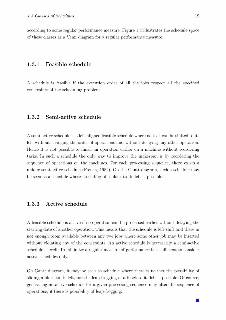
according to some regular performance measure. Figure 1.4 illustrates the schedule space

of these classes as a Venn diagram for a regular performance measure.

1.3.1 Feasible schedule

A schedule is feasible if the execution order of all the jobs respect all the specified

constraints of the scheduling problem.

1.3.2 Semi-active schedule

A semi-active schedule is a left-aligned feasible schedule where no task can be shifted to its

left without changing the order of operations and without delaying any other operation.

Hence it is not possible to finish an operation earlier on a machine without reordering

tasks. In such a schedule the only way to improve the makespan is by reordering the

sequence of operations on the machines. For each processing sequence, there exists a

unique semi-active schedule (French, 1982). On the Gantt diagram, such a schedule may

be seen as a schedule where no sliding of a block to its left is possible.

1.3.3 Active schedule

A feasible schedule is active if no operation can be processed earlier without delaying the

starting date of another operation. This means that the schedule is left-shift and there in

not enough room available between any two jobs where some other job may be inserted

without violating any of the constraints. An active schedule is necessarily a semi-active

schedule as well. To minimize a regular measure of performance it is sufficient to consider

active schedules only.

On Gantt diagram, it may be seen as schedule where there is neither the possibility of

sliding a block to its left, nor the leap frogging of a block to its left is possible. Of course,

generating an active schedule for a given processing sequence may alter the sequence of

operations, if there is possibility of leap-frogging.

�


Non-delay

Semi-active

Active

Feasible

Optimal

Figure 1.4 – Classes of Schedules

1.3.4 Non-delay schedule

A schedule is called non-delay if no machine is kept idle while an operation is waiting for

being processed on that machine. A non-delay schedule is necessarily an active schedule

and hence semi-active as well.

1.3.5 Optimal schedule

An optimal schedule is a schedule that gives the best possible value for some given perfor-

mance measure. There may be more than one optimal schedules for the same performance

measure. For more than one objective, the sense of optimality is quite different as explai-

ned in § 1.2.4. Note that at least one optimal schedule is active, however there need not

be an optimal schedule, which is non-delay.

Consider an example of a single machine problem with three single-operation jobs as given

in Table 1.3. Figure 1.5 illustrates these classes of schedules for this simple problem.

Schedule σ1 (Figure 1.5(a)) is not a semi-active schedule, because job 1 starts at t = 10,

j rj pj

1 0 4

2 2 3

3 4 4

Table 1.3 – An example problem to illustrate classes of schedules

�

1.3 Classes of Schedules 21

0 1 2 3 4 5 6 7 8 9 10 11 12 13 14 15

M1 2 3 1

(a) σ1: Non Semi-active schedule

0 1 2 3 4 5 6 7 8 9 10 11 12 13 14 15

M1 3 2 1

(b) σ2: Semi-active schedule

0 1 2 3 4 5 6 7 8 9 10 11 12 13 14 15

M1 2 3 1

(c) σ3: Active schedule

0 1 2 3 4 5 6 7 8 9 10 11 12 13 14 15

M1 1 2 3

(d) σ4: Non-Delay schedule

Figure 1.5 – Schedules of the problem described in Table 1.3

that could have started at t = 9 without violating any constraint, and without changing

the execution order of jobs on the machine. Since this ordering is not semi-active, it is

neither active nor non-delay.

Schedule σ2 (Figure 1.5(b)) is a semi-active schedule as no job can be slid towards its

left without reordering the tasks. It is not an active schedule. In fact, if job 3 is at first

position, the schedule can never be active as there will always be a room for job 1 before

job 3. As it is not active, so it is also not non-delay.

Schedule σ3 (Figure 1.5(c)) is an active schedule (and a semi-active as well) because no

job can be shifted towards its left without delaying other tasks. It is however, not a non

delay schedule as job 1 could have been processed on machine at t = 0, but machine is

kept idle.

Schedule σ4 (Figure 1.5(d)) is a non-delay (as well as active and semi-active) as machine

is never kept idle when a job was available.

�


1.4 Classification and Notations of Scheduling Pro-

blem

Based on the job arrival process, scheduling problems in which number of jobs are known

and fixed with all jobs having the same ready times are referred as static problems in

contrast to the dynamic problems in which jobs are continually revealed during the exe-

cution process (French, 1982).

Scheduling problems with all the variables describing the problem data (e.g. process times)

are known a priori are termed as deterministic problems in contrast to stochastic schedu-

ling problems where these variables are probabilistic in nature.

Scheduling problems can have single stage and multi-stage environments. In a single stage

environment, each operation goes through one machine only. In a multi-stage environment,

an operation can be executed by one of the machines of the same stage, so a machine has

to be selected first to perform the operation (Pinedo and Chao, 1999).

There are different notations used to classify scheduling problems. (Conway et al., 1967)

formulated a four field notation, A/B/C/D which is suitable for basic scheduling pro-

blems. In this notation, the field A represents number of jobs, B represents number of

machines, C represents the shop environment and D represents the scheduling objective.

MacCarthy and Liu (1993) improved this notation by proposing several modifications to

C descriptor. Graham et al. (1979) proposed a three field notation α, β and γ. This is the

most used descriptive method to represent a scheduling problem.

1.4.1 α field:

The α field describes the machine environment. It consists of α1 and α2 where α1 is the

type of shop and α2 is the number of machines in the problem and is optional. If this field

is empty, then the number of machines is the data of the problem. Some notations of α

field are given in Table 1.4.

Machine environments can be classified in two categories. In the first category, each job

requires one and only one machine. Single machine, identical parallel and unrelated parallel

machine environments fall into this category. In the second category, there are m different

work-centers with each work-center consisting of one or many parallel machines. Each

job Jj ∈ J consists of a set of operations Oj. Depending upon the routing policy of

�

1.4 Classification and Notations of Scheduling Problem 23

Table 1.4 – Some examples for the field α

α Description

φ Single machine, the value for the field α is “1”

Pm m Identical parallel machines

Qm m Parallel machines with different speeds

Rm m Unrelated parallel machines

Fm m machine flow shop

FFc c stages in series as a flow shop with each stage as Pm or Qm

Fπm Permutation flow shop of m machines

Jm m machine job shop

FJc c work-centers with each work center as Pm or Qm

Om m machine open shop

these operations on the machines, three different classes of machine environments can be

identified.

Flow shop

All jobs are to be processed sequentially on multiple machines where each job has to follow

the same route. Figure 1.6 demonstrates a three machine flow shop. A generalization of

flow shop is the flexible flow shop that consists of a number of stages in series with a

number of machines in parallel at each stage. There exist many variants of the flow shop

e.g. zero-buffer flow shop, flow shop with blocking, no-wait flow shop and the hybrid flow

shop. Academic research, however is more focused on a simplified version of flow shop, the

permutation flow shop where jobs are to to be processed in the same sequence by each of

the machine. A permutation flow shop is illustrated in Figure 1.7.

{J }nj=1 M1 M2 M3...

Figure 1.6 – A three machine flow shop, F3

Job shop

In a job shop, each job has its own predetermined route to follow. It is a generalization

of a flow shop (A flow shop is a job shop in which each job has the same route). Job shop

�


M1 M2 M3...

J3

J1

J2

J3

J1

J2

J3

J1

J2

Figure 1.7 – A three machine permutation flow shop,F3|prmu|−

has a special precedence relation of the form Oj1 → Oj2 → Oj3 → . . .Ojoj ,∀j ∈ J . A

generalization of the job shop is the flexible job shop with work-centers that have multiple

machines in parallel. Each job visits each machine at most once, however in a variant of

job shop, called recirculation job shop, a route may not go through all machines however

a job may have multiple visits on a machine for execution of its operations. The latter

case is represented by a rcrc entry in the β-field. A flexible job shop with recirculation is

considered the most complex machine environment from combinatorial point of view, and

is very common in semiconductor industry (Pinedo and Chao, 1999). Figure 1.8 illustrates

a simple job shop with three machines.

J1 M1

M2

M3

J2

J3

J1 : M1 M2 M3

J2 : M2 M1 M3

J3 : M3 M2

Figure 1.8 – A three machine job shop, J3

As in this study we focus on job shop problem, a detailed description of the job shop is

�

1.4 Classification and Notations of Scheduling Problem 25

given in § 1.6.

Open shop

In an open shop, there is no predefined sequence of operations among jobs i.e. jobs do

not have a predefined routing, instead it is established during the scheduling.

In a mixed shop, the machine routes of jobs can either be fixed or unrestricted. It can be

regarded as a mix of aforementioned shops.

1.4.2 β field:

The β field describes the constraints and particularities of the problem. For example:

Deadline These are imperative due-dates. A deadline is a due date for which tardiness

is not allowed.

Preemption Processing of a job on a machine may be interrupted and resumed at a

later time even on a different machine and already processed amount is not lost.

Precedence One or more jobs have to be completed before another job is allowed to

start.

Release Date The release date of job Jj, is the time when a job is arrived at the system

to be processed and the job cannot start its processing before release date.

Some possible entries of β field and their notations are given in Table 1.5.

Any other entry that may appear in the β field is self-explanatory. For example, pj = p

implies that all processing times are equal and dj = d implies that all due dates are equal.

Due dates, in contrast to release dates, are usually not explicitly specified in this field;

the type of objective function gives sufficient indication whether or not the jobs have due

dates.

1.4.3 γ field:

The γ ∈ {fmax,∑

f} field describes the objective function and is similar to the D des-

criptor of the notation of Conway et al. (1967).

�


Table 1.5 – Some examples for the field β

β Value Description

β1pmtn, φ

pmtn: preemption is allowed

φ: preemption is not allowed

β2res♯, φ

res♯: ♯ limited number of resources

φ: no resource limitation

β3

prec, tree, φ

prec: a precedence relation between jobs is speci-fied

tree: a tree like precedence relation between jobsis specified

φ: no precedence relation

β4rj, φ

rj: release dates are specified

φ: ∀j, rj = 0

β5J 6 p, φ

J 6 p: all jobs have at most p operations

φ: no restrictions on size of jobs

β6

pjk = 1, a 6 pjk 6 b, φ

pjk = 1: each operation has a unit processing time

a 6 pjk 6 b: processing time of each operation hasa lower bound a and an upper bound b

φ: no restriction on processing times

Table 1.6a – Some examples for the field γ

γ Description

Cmax Makespan

Tmax Maximum tardiness

ΣjTj Total tardiness

T Mean tardiness

Some are given in Table 1.6a. For multi-objective problems, list of objectives separated

by comma are used in γ field. For instance, a single machine problem with Cmax and T

can be noted as 1||Cmax,T . Moreover, based on the method to compute Pareto optimum,

different values for the γ field can be introduced, as shown in Table 1.6b.

�

1.5 Scheduling Phases 27

Table 1.6b – Some MO examples for the field γ

γ Description

♯(f1,...,fK) Enumeration of non-dominated solutions

Lex(f1,...,fK) Lexicographic optimisation of K objectives

Fl(f1,...,fK) Convex combination of K objectives

ǫ(f1,...,fK) ǫ-constraint method of K objectives

1.5 Scheduling Phases

1.5.1 Predictive Phase

The phase of a scheduling method that takes place before the actual execution of the

schedule is referred as predictive phase. This phase of the scheduling method is generally

not time constrained in terms of finding the solution and is applied to the model of the

real system as an off line method.

1.5.2 Reactive Phase

The reactive phase of a scheduling method takes place during the execution of the schedule.

The scheduling method during this phase, therefore can observe the occurrence of actual

events of the system. However the scheduling method during this phase must not be too

time consuming.

1.6 Job Shop Scheduling Problem

Our focus in this study is on a specific scheduling environment, namely job shop. Here we

shall describe the formal definition of a job shop scheduling problem (JSSP), graphical

representation, its complexity, different benchmark problems and a brief overview of

resolution approaches for JSSP.

�


1.6.1 Formal definition of JSSP

The job shop scheduling problem with multiple precedence constraints is a combinatorial

optimization problem composed of a finite set J of n jobs {Jj}nj=1 to be processed on a fi-

nite setM ofm resources {Mk}mk=1. A job Jj consists of a sequence Oj = (Oj1,Oj2,...Ojoj)

of oj operations with each operation Ojk as part of exactly one job Jj to be processed

during a processing time pjk > 0 on a resource Mk. A resource can execute only one

operation at a time. Solving a job shop problem is the task of assigning each operation,

a specific position on the time scale of specified machine while optimizing a set of given

performance measures (Conway, 1965b).

Generally size of the JSSP is given as m × n. An instance of a JSSP is given in table

Table 1.7.

Job rj machine sequence pjk

J1 0 M1, M2, M3 p11=10, p12=8, p13=4

J2 0 M2, M1, M4, M3 p22=8, p21=3, p24=5, p13=6

J3 0 M1, M2, M4 p31=4, p32=7, p34=3

Table 1.7 – An instance of a JSSP

1.6.2 Graphical Representation

1.6.2.1 Gantt Diagram

Gantt diagram is a very simple and extensively used tool to graphically present the exe-

cution order and timings of tasks on the machines throughout the time horizon. Gantt

diagram can be machine-oriented or job-oriented. In this study, all the Gantt diagrams

will be machine-oriented. An example of a machine-oriented Gantt diagram is shown in

Figure 1.9 for an arbitrary feasible solution for the problem instance given in Table 1.7.

1.6.2.2 Disjunctive Graph

Although Gantt diagram is an excellent monitoring tool of a schedule, it is inca-

pable of representing the problem itself. Disjunctive graph representation proposed by

(Roy and Vincke, 1981) is able to effectively represent a scheduling problem.

�

1.7 Solving Methods 29

0 1 2 3 4 5 6 7 8 9 10 11 12 13 14 15 16 17 18 19 20 21 22 23 24 25 26 27 28 29 30 31 32 33

M1 J3 J1 J2

M2 J2 J3 J1

M3 J2 J1

M4 J2 J3

Figure 1.9 – Gantt diagram for a schedule for the problem in Table 1.7.

A disjunctive graph is a 3-tuple G=(V,C,D) with V as set of vertices representing the set

of operations O and two special vertices as a source node and a terminal node, C as set

of conjunctive arcs representing the given precedence constraints between the operations

of the same job, and set of disjunctive arcs by D={{u,v}|u,v ∈ O,u 6= v,M(u) = M(v)}

represent the machine capacity constraints. Each arc has a weight, equal to the processing

time of the operation corresponding the vertex from which the arc emits. Figure 1.10

illustrates a disjunctive graph for a job shop problem with four machines and three jobs as

given in Table 1.7. For even a slightly larger problem, the disjunctive graph representation

gets too complicated to visualize. A relatively simplified version the disjunctive graph,

where instead of inter-connecting all the operations of the same machine by disjunctive

arcs, only one disjunctive arc is drawn, may be used (as shown in Figure 1.11). By setting

the direction of each arc such that there are no cycles in the disjunctive graph, a solution

to the problem is represented, as shown Figure 1.12.

O11 O12

p11O13

p12

O22 O21

p22O24

p21O23

p24

O31 O32

p31O34

p32

O⋄⋄

r1

r2

r3

O⋆⋆

p13

p23

p34

Figure 1.10 – Disjunctive graph representation of problem in Table 1.7

1.7 Solving Methods

There has been extensive research in a plethora of methods to solve JSSP. These methods

can be classified in three broad classes of exact, heuristic and AI based methods. An

excellent survey on these methods is presented by (Jain and Meeran, 1998). A brief review

�


O11 O12

p11O13

p12

O22 O21

p22O24

p21O23

p24

O31 O32

p31O34

p32

O⋄⋄

r1

r2

r3

O⋆⋆

p13

p23

p34

Figure 1.11 – Simplified Disjunctive graph representation of problem in Table 1.7

O11 O12

p11O13

p12

O22 O21

p22O24

p21O23

p24

O31 O32

p31O34

p32

O⋄⋄

r1

r2

r3

O⋆⋆

p13

p23

p34

Figure 1.12 – Disjunctive graph representation of solution

of different methods is presented in this section.

1.7.1 Exact methods

Exact methods are guaranteed to find an optimal solution for a finite size instance of

a combinatorial optimization problem in a bounded time. However, for a typical com-

binatorial optimization problem like JSSP, no algorithms exist to solve these problem

in polynomial time (Conway et al., 1967; French, 1982). Enumerative methods such as

branch and bound algorithms, mathematical programming (Integer Linear Programming

(ILP) and Mixed Integer Linear Programming (MILP)) are the most well-known methods

to solve scheduling problems like JSSP. Branch and bound methods are very sensitive

to individual instances and the initial bounds used. They are found to be unsuitable for

larger instances.

1.7.2 Approximation methods

The computational complexities required by exact methods lead the research to approxi-

mation methods. Solutions by such methods are obtained in reasonable computational

�

1.7 Solving Methods 31

times, however these are not guaranteed to be optimal. These can be divided into construc-

tive and iterative methods.

1.7.2.1 Constructive methods

In these methods, the schedule is generated gradually by adding schedulable operations to

an initially empty schedule. Priority dispatching rules (pdrs), such as First In First Out

(FIFO) and Earliest Due Date (EDD) etc. are among the most widely used constructive

heuristics for shop scheduling problems due to their ease of implementation and substan-

tially lower computational requirements. They give inferior quality schedules in general,

however some pdrs generate optimum schedules for some simple problems. There does not

exist a single rule that can be applied to all shop problem with a satisfying performance.

Moreover, it is not possible to estimate the performance of a pdr for a specific instance a

priori (Zobolas et al., 2008).

Shifting Bottleneck (SB) heuristic have been a very effective heuristic in job shop schedu-

ling. In SB heuristic, several single machine problems are solved to optimality. Bottleneck

machine is selected first for the optimization, where bottleneck machine is defined as

the machine having longest makespan as its optimum. The algorithm continues until all

machines are scheduled.

1.7.2.2 Iterative Methods

Iterative methods such as meta-heuristics efficiently and effectively explore the search

space driven by logical moves and knowledge of the effect of the move facilitating the

escape from locally optimum solutions (Blum and Roli, 2003). Two important ways to

classify the meta-heuristics are population based vs single point search and memory based

vs memory-less meta-heuristics (Jain and Meeran, 1998).

Most known meta-heuristic algorithms applied to JSSP include evolutionary algorithms

(EA), particle swarm optimization (PSO), ant colony optimization (ACO), scatter search,

exploratory local search, neural networks, simulated annealing (SA) and tabu search (TS).

Population based meta-heuristics work simultaneously on a set of solutions. Genetic al-

gorithms are the most important representatives of this class among others concerning

the literature on JSSP. However, Genetic algorithms are not found to be suitable for fine-

tuning of solutions close to optimal (Zobolas et al., 2008). PSO and ACO did not find any

significant success as well in this domain, except when hybridized with other methods.

�


Simulated annealing (SA) is one of the earliest proposed meta-heuristic. However, it is

unable to quickly achieve good solutions to JSSP. This is generally attributed to its generic

nature and memory-less functionality.

Tabu search has been shown to be a very powerful meta-heuristic for JSSP

(Nowicki and Smutnicki, 1996; Jain and Meeran, 1998; Watson et al., 2006;

Zobolas et al., 2008; Zhang et al., 2008). The main characteristic of tabu search is

its memory-usage which is an indication of intelligence employed during the search

process.

1.8 Conclusions

In this chapter, the basic notions of the scheduling domain are presented. More specifically,

the problem of job-shop is presented with its variants and representation schemes. Like

most of the real-world scheduling problems, job shop problem is NP-hard with a very few

exceptions. To solve job shop problems, numerous techniques have been applied belonging

to the category of either exact methods or approximate methods and in nature either

constructive or iterative. However, none of these methods is capable to show its supremacy

over others in all desired aspects of solving the problem. On one side, some of them are

too time-consuming to be adopted or very specific to the environment while on the other

hand, some of the methods perform very poorly despite being fast and/or generic. In the

next chapter, we present a review of a very important class of methods, called priority

dispatching rules, that gained much attraction of the researchers due to their extensive

use in real-time systems and ease of implementation.

�

2A State of the Art

Survey of Priority

Dispatching Rules

2.1 Introduction . . . . . . . . . . . . . . . . . . . . . . . . . . . . 33

2.2 Classification of Priority Dispatching Rules . . . . . . . . . . . 35

2.2.1 Structure Based Classification . . . . . . . . . . . . . . . . . . . . . . . . 35

2.2.2 Information Based Classification . . . . . . . . . . . . . . . . . . . . . . 35

2.3 Literature Reviews on Priority Dispatching Rules . . . . . . . 38

2.4 Priority Dispatching Rules . . . . . . . . . . . . . . . . . . . . 41

2.5 Comparative Studies and Important Factors . . . . . . . . . . . 48

2.5.1 A Review of Comparative Studies on PDRs . . . . . . . . . . . . . . . . 48

2.6 Factors Affecting Performance of PDRs . . . . . . . . . . . . . 50

2.6.1 Load Variation . . . . . . . . . . . . . . . . . . . . . . . . . . . . . . . . 50

2.6.2 Due Date Variation . . . . . . . . . . . . . . . . . . . . . . . . . . . . . 51

2.6.3 Method of Assigning Due Dates . . . . . . . . . . . . . . . . . . . . . . . 51

2.7 Conclusions . . . . . . . . . . . . . . . . . . . . . . . . . . . . . 52

For real-time management of waiting-lines in manufacturing system, priority dispatching

rules appear to be the most frequently used method. Over the years, numerous dispatching

rules have been proposed by the researchers. This chapter provides a survey of priority

dispatching rules that have been extensively used by researchers and practitioners. All the

rules presented in this chapter are described in Annex A.

2.1 Introduction

Although approximation methods to solve job shop scheduling problem do not guarantee

achieving optimal solutions, they are able to attain acceptable solutions within moderate

computing times and are therefore more suitable for larger problems. Koulamas (1994)

34 Chapter 2. A State of the Art Survey of Priority Dispatching Rules

states that there is abundant of optimization procedures available for a variety of stan-

dard scheduling environments such as single-machine, flow shop and job shop settings.

However, these procedures are generally limited to static problems of relatively smaller

in size (Panwalker and Iskander, 1977). Hence, more scheduling research introducing effi-

cient heuristics has been called for especially for large-size dynamic problems. According

to (Jain and Meeran, 1998), approximation procedures applied to job shop scheduling pro-

blem were first developed on the basis of priority dispatching rules (pdrs). Many different

terms such as priority rule, dispatch heuristic, and scheduling rule are used to refer to the

principles that determine the relative importance of a job among all waiting jobs when

selecting the next one for processing without inserting idle time. However, it is possible in

practice that some idle time is inserted in the schedules while waiting for a soon-to-arrive

urgent job instead of prioritizing back-logged jobs.

In the dispatching approach, each machine is loaded as soon as there is at least one

job awaiting service in front of the queue, eliminating any unnecessary idle time of the

resources. At each successive step all the operations which are available to be scheduled

are assigned a priority index and the operation with the highest priority index is chosen

to be sequenced. In most of the cases, this is referred as implicit scheduling decision based

approach, where the impact of each dispatching decision on the completion times of other

jobs is not monitored (Kemppainen, 2005).

The general approach for a dispatching rule, according to (Montana, 2005), is to define

a score associated with assigning a given task to a given resource and select the eligible

task that minimizes (or maximizes) that score for the chosen resource. (Haupt, 1989)

defines it as a policy with a specific sequencing decision, applied each time a resource gets

idle. According to him, priority rule-based scheduling approach considers the sequencing

decision as a set of independent decentralized one-machine problems.

A priority dispatching rule (pdr) determines a value of priority index, κj, for any job Jj

in a given scheduling situation, and of a ranking procedure using the priority indices for

selecting one of the schedulable jobs waiting on an idle machine to be started next (Baker,

1974; Panwalker and Iskander, 1977).

Dynamic scheduling uses dispatching rules to prioritize jobs waiting for processing at a

resource (Vieira et al., 2003). Due to their ease of implementation and their substantially

reduced computational requirement they remained a very popular technique despite of

their poor performance in the long run (Baker, 1974; French, 1982; Morton and Pentico,

1993). This approach is best when there is on-line scheduling (i.e. tasks being revealed

during execution), the fundamental time scale of the problem is short, and the future is

very uncertain (Montana, 2005).

�

2.2 Classification of Priority Dispatching Rules 35

This chapter provides a state-of-the-art review on priority dispatching rules in context

with job shop scheduling environment. In § 2.2, we present frequently used classification

schemes for pdrs found in literature. In § 2.2, different pdrs have been discussed. In the

next section a comparative analysis of these pdrs is made. In the last section we draw

some concluding remarks.

2.2 Classification of Priority Dispatching Rules

For identifying the characteristics and making a comparative study of the behavior of

different priority dispatching rules, it is important to classify the priority dispatching

rules. A number of classifications of pdrs have been presented in the literature that help

to improve the understanding of the status of research in this area. Generally, structural

based, information based or performance measure based classifications of pdrs are found

in literature. However, the classification is not unique as some pdrs may fall in multiple

classes.

2.2.1 Structure Based Classification

A structure based classification (Panwalker and Iskander, 1977) divides the pdrs in three

broad classes namely, basic rules, heuristic scheduling rules and other rules. Basic rules are

further categorized as simple, composite and weighted priority rules. Simple rules typically

use job-specific information like processing times, due dates or the queue length at next

machine for the job. The composite rules apply different pdrs to certain groups of jobs or

use different pdrs depending on the shop status and circumstances. The weighted prio-

rity rules combine different simple or composite rules by assigning parameterized weight

to each rule. The heuristic scheduling rules, such as CEXSPT, (although not considered

as pdrs by (Panwalker and Iskander, 1977)) involve a relatively complex consideration of

situations such as anticipated waiting times on subsequent machines and the effect of al-

ternate job routing etc. They may also include non-mathematical aspects such as inserting

a job in an idle time slot by visual inspection (Kemppainen, 2005). Other rules include

rules designed for specific shop, combination of priority indexes based on mathematical

functions of job parameters or those that are not categorized earlier.

�


2.2.2 Information Based Classification

Information based classification divides the pdrs in three classes based on information

content (Blackstone et al., 1982), scope and detail of information and time dependency.

Based on the Information Content

Pdrs based on individual piece of information related to job, queue or resource may be

grouped in the information content based class.

Based on the Scope and Detail

Scope and detail based classification groups the pdrs in local and global pdrs

(Hausman and Scudder, 1982). The rule is local, if the priority index is based on the

information of the current machine, queue and/or the attributes of the jobs in the queue

of current machine only. On the other hand, a global rule uses information concerning the

status of the shop, such as the length of the current queue relative to the average queue

length in the shop or system load etc. A global rule may further be sub-divided as indirect

global and direct global, based on how the global information is obtained (Vepsalainen,

1984). For indirect global pdrs, the information is derived from aggregate system indica-

tors (e.g. distribution of processing times) without any explicit reference to the attributes

of the specific jobs to be scheduled on subsequent machines. In contrast, direct global

rules use explicit, observable or anticipated global information pertaining to specific jobs

(e.g. queue length on the next machine).

Based on the the Horizon of Information

Based on the horizon of information, a pdr can be static or dynamic. For a static pdr,

priority index is fixed when the job is introduced and hence it is based on the initial data

only. So for a static rule, the information on which the priority index is assigned, is not

changing over time and for on-going scheduling process, it may be seen as information

from past. Dynamic priority index depends on the actual evolution of the system and

cannot be computed in advance (Moser and Engell, 1992). So for dynamic pdrs (some

of) the information content used to assign priority index is changing over time. However,

this information is from observable status of the shop only without any forecasting (hence

referred as myopic dynamic pdrs).

The concept can be extended to take future information by forecasting as well and then

providing a feedback for current scheduling decision to be made. On the basis of type of

�

2.2 Classification of Priority Dispatching Rules 37

information feedback, (Vepsalainen, 1984) divided the dynamic pdrs as anticipated status

feedback and performance feedback.

Anticipated status feedback The anticipated status of the shop in the future is used as

feedback, for example average queue lengths estimated through aggregate forecasts

or detailed forward simulation.

Performance feedback The anticipated performance of the rule over some forecasting

horizon is used as feedback to adjust its parameters .

Moser and Engell (1992) have classified the rules as being a-priori and a-posteriori, where

in a-priori rules the priority index is computed from jth operation alone in contrast to a-

posteriori rule which considers the situation which would arise if jth operation is scheduled

as the next operation. A-posteriori rules can be seen as general dynamic pdrs with feedback

(usually obtained by repeated forward simulations) .

Kutanoglu and Sabuncuoglu (1999) have classified pdrs into two categories: (1) single-pass

and (2) multi-pass. In single-pass heuristics, a single complete solution is built up one step

at a time. Most priority dispatching rules proposed in the literature can be considered in

this category. In multi-pass heuristics, an initial schedule is generated in the first pass,

and then the consecutive passes search, for improvement in performance e.g. iterative

dispatching.

The generic rules, that are not specific to a particular manufacturing facility, are classified

using a matrix form by (Kemppainen, 2005) where it is assumed that the positioning of a

rule within the classification predicts its performance as a coordinative mechanism, shown

in Figure 2.1. These categories are briefly described below.

Priority index fixed on entry based on job-specific information The pdrs re-

lying on static data typically use information on job attributes only. Examples

of such rules include earliest due date(EDD), number of operations (NOP), and

first come first served (FCFS). Some composite rules like average processing time

AVPRO also fall in this category.

Priority index fixed on entry using operations detail information SI, FIFO and

operational due date (ODD) rules fall in this category. Also there are other rules,

which can be implemented with operation-specific information.

Priority index fixed on entry using load and resource information Priority dis-

patching rules that use information about the machine for which the dispatching

decision is done fall in this category. For example, the value of the shortest setup

(SST) rule depends on both the machine and imminent operation.

�


Priority index updated by stage using job-specific information Many of the ge-

neric dispatch priority rules are stage-update-able, i.e. priority index values are

time-dependent. Examples include the modified due date (MDD) rule and SLACK

rule.

Priority index updated by stage using operations detail information This ca-

tegory includes several composite rules such as the process time plus process wait

(PT+PW) rule, CR/SI , S/RPT+SPT (Anderson and Nyirenda, 1990) and the dif-

ferent versions of the SLACK rule e.g. slack per number of operations (S/OPN), slack

per time allowable (S/RAT), and slack per remaining processing time (S/RPT).

Priority index updated by stage using load and resource information

Examples of dispatch priority rules that use information about the entire

production system in the calculation of job-specific priority values are the work in

the next queue (WINQ) and the number of jobs in the next queue (NINQ) rules.

The PT+WINQ rule introduced by (Holthaus, 1997) prioritizes jobs with the least

work in the current operation and lowest expected load in the next operation.

Priority index adapted by probing and job attribute information None of the

generic dispatch priority rules fall in this category. There are, however, modifications

of the conventional dispatching rules such as the high response ratio (HRN) rule by

(Selladurai et al., 1995) and the shortest expected processing time (SEPT) rule by

(Wein and Chevalier, 1992) that anticipate the processing and waiting times of jobs.

Priority index adapted by probing and operations detail data By controlling

the scheduling of jobs with long processing times and by employing both job-

based and operation-based due date information to expedite late jobs the CEXSPT

rule decreases the undesirable property of SPT that results in some very late jobs

(Schultz, 1989).

Priority index adapted by probing and load and resource information The

classification of two integrated trade-off heuristics COVERT and ATC rules,

depends on the lead time estimation method used. If job-specific lead times are

estimated using a multiple of processing time, the rules can be positioned to

category of pdrs that are updated by stage using operations detail information.

With lead time iteration these methods should be classified into this category.

�

2.3 Literature Reviews on Priority Dispatching Rules 39

EDD,NOP,FCFS

SPT,LPT,ODD

SST

MDD,SLACK

CR, MOD,S/OPN,CR/SI,

S/RPT+SPT

WINQ,PT+WINQ

CEXSPTBD,

MF, RR,Emery’sRule

Adaptedby probing

Updatedby stage

Fixedon entry

Jobattributes

Operationdetail

Load/Resources

COVE

RT,

ATC

Figure 2.1 – Classification Matrix of PDRs, adapted from (Kemppainen, 2005)

2.3 Literature Reviews on Priority Dispatching

Rules

The earliest work on pdrs was done by (Jackson, 1955, 1957; Smith, 1956;

Rowe and Jackson, 1956; Sisson, 1959; Giffler and Thompson, 1960; Baker and Dzielinski,

1960; Gere Jr, 1966). The algorithm of Giffler and Thompson (1960) is the common basis

of all pdrs and its importance is derived from the fact that it generates active schedules.

In active schedule, the processing sequence is such that no task can be started any earlier

without delaying some other task or violating the technological constraints. The procedure

commences by choosing a yet to be sequenced operation, Ojk, with the earliest completion

time, then it finds all the other operations that use the same machine Mk and which start

earlier than the completion time of Ojk. These operations are placed in a conflict set. An

operation is then selected from the conflict set and sequenced as early as possible. The

procedure is repeated until all operations have been sequenced. Pdrs are characterized by

the method applied to select operations from the conflict set where a random choice is

the simplest priority assignment.

Jackson (1955); Moore (1968) have presented the earliest reviews on the simulation of job

shop, discussing the use of priority dispatching rules.

�


Table 2.1 – Relevant Literature Review on PDRs

Reference Conditions Performancemeasures

Pdrs tested a

Schultz (1989) Job Shop, TWK b,η c=80%,90%

T , CMT , %T CEXSPT, MOD, COVERT, SPT,ODD, S/OPN, OCR

Moser and Engell (1992) T , Trms, Tmax WLS, ODD, CR, SL/OPN,CR+SPT, SPT-T, COVERT,WINQ

Raghu and Rajendran (1993) Open shop TWK withallowance factor of 4,5,6η=85%,95%

T , Trms, %T RR, SPT, EDD, MOD, ATC ,S/RPT + SPT, CR+SPT

Chang et al. (1995)

Holthaus (1997) TWK with allowancefactor of 2,4,6,8 η=85%,90%, 95%

T , Tmax, %T ,σ2T

AT, AT-RPT, FIFO, SPT,WINQ, RR, RAN(SPT,WINQ),PT+WINQ, PT+WINQ+SL,(PT+WINQ)/TIS

Kutanoglu and Sabuncuoglu(1999)

Job shop RATWK with6,9,12 η=60%, 80%, 90%

T FCFS, WSPT, WLWKR,EDD,MDD, SLACK, CD, S/OPN,MDSPRO, ODD, OSLACK,OCR,MOD, CEXSPT, W(CR+SPT),W(S/RPT+ SPT),COVERT

Horng and Chou (2002) η=80%, 90% TWK with4, 6

T , Tmax, %T ,σ2T

SPT, RR ,PT+WINQ, AT-RPT,PT+WIND+AT,PT+WINQ+AT+SL,PT+WIND+SL

Dominic et al. (2005) MF, SPT, EDD, WeightedCOVERT, ATC

Kemppainen (2005) Job shop RANSLK(0-6)η=85 %, 95%

T , Tmax, %T EDD, CR, ODD AVPRO, SPTSLACK, S/OPN, S/RPTAT-RPT, OPSLK/PT, ODD,PT+PW ATC, COVERT,CR+SPT, PT+WINQ,PT+WINQ+SL, RR,S/RPT+SPT

Weng and Ren (2006) Job shop TWK with 6,12η=80%, 85%, 90%, 95%,97%

T WR, FCFS, EDD, SPT,COVERT, ATC

Chiang and Fu (2007) T , Tmax, %T SPT, SRPT, LTWK, SPT/TWK,SLACK, EDD, MDD, ODD,MOD, COVERT, ATC,CR,PT+PW, PT+PW+ODD,WINQ, PT+WINQ+SLACK

a see § 2.4 and Annex Ab see § 2.6.3c Shop Utilization

Later on, (Conway et al., 1967; Jones, 1973; Holloway and Nelson, 1974; Baker, 1974)

provided thorough reviews of various dispatching rules and their performance in different

�

2.4 Priority Dispatching Rules 41

circumstances. However, (Panwalker and Iskander, 1977) has provided a most compre-

hensive survey of scheduling heuristics presenting 113 pdrs. They reviewed and classified

these pdrs along-with information about the scheduling environment and performance

measures used in earlier surveys. They concluded that in many cases, the results were

found conflicting due to difference in operating conditions and the underlying assump-

tions. They also observed that there are many rules that assign the same priority to two

or more jobs waiting to be processed, requiring their use in conjunction with other rules,

possibly as tie-breaking rules.

Blackstone et al. (1982) provide an extended discussion and summary of 34 pdrs, mostly

used in literature and industrial practice. They discussed various factors that influence

the performance of pdrs as well. In addition, a brief review of the ”‘secondary dispatching

heuristics”’- procedures that may be used to identify circumstances under which the job

selected by a dispatching rule should not be processed first.

Haupt (1989) reviewed 26 different pdrs (and a few pdrs for extended job shop en-

vironments), while classifying them based on the scope and time horizon. They also

described two standard procedures of combining the simple pdrs, namely additive and

alternative combinations, with a particular importance to the appraach proposed by

(O’Grady and Harrison, 1985).

Chan et al. (2002) provides a state-of-the art on different scheduling strategies using si-

mulation. They reviewed a number of publications on the use of pdrs, specifying the job

configurations used by the authors.

In the next section, we present some of the most used pdrs in practice as well as in

literature.

2.4 Priority Dispatching Rules

In this section, a few well-known pdrs - that have been extensively used in experimental

or analytical studies on scheduling- are discussed. The names of the rules may not be the

same as the names used by many researchers.

The FIFO (First In First Out) rule is considered to be a fair priority rule, especially in

service operations and extensively used as a benchmark rule in literature. It is expressed

as minj(Cj(i−1)). Job based version of the rule is FCFS (First Come First Served) and is

expressed as (minj(rj)).

�


SI 1 (Shortest Imminent) rule is probably the most widely tested pdr in literature. Conway

(1965a) was the first to summarize that it should be considered as the standard benchmark

for all dispatching studies, even though in his experiments the rule did not exhibit the

minimum value for any of the performance measures including average queue length and

average work-in-process measured with total work. The rule is expressed as, minj(pjk).

Obviously it requires a single, yet the most important piece of information, the processing

time from the local queue only.

In case of a single machine static problem, it minimizes the mean flow-time (maximizes

throughput), mean lateness (Conway, 1965a; French, 1982; Blackstone et al., 1982) and

for all due-dates to be equal or all jobs are to be inevitably finished late, this rule minimizes

T as well (Moser and Engell, 1992).

This rule performs well with externally set due dates in general. For internally set due

dates using TWK method (see § 2.6.3), it is found to be better than due date based rules

if due dates are set at less than seven times total processing time (Elvers, 1973). The rule

is found to be least sensitive to the due-date assignment method (Conway, 1965a) and

forecasting errors in due dates as well (Eilon and Hodgson, 1967). The major drawback of

this rule is that some jobs become very late. This results in a very high value for maximum

tardiness, Tmax and variation of the tardiness.

Eilon and Cotterill (1968); Eilon and Choudury (1975) proposed a modification of the SI

rule called the SIx rule, in order to alleviate the disadvantage of holding some jobs quite

long in the queue by SI. Two separate queues with one having priority over the other are

formed with both queues ranked by SI rule. Jobs with slack less than a control parameter,

Q (same for all jobs) are placed in the priority queue. Although the rule reduces the

variance of missed due-dates as compared to SI, the authors do not report testing the

rule against other tardiness-orientated rules, nor do they provide guidance for selecting Q

based on factors such as due-date tightness, shop utilization or the method of assigning

due-dates.

Oral and Malouin (1973) developed a similar rule, known as the SPT-T rule. The rule

combines the SI and S/OPN (defined later) rules in such a way as to retain the advantages

of both while avoiding their disadvantages. Specifically, a job’s priority is given by the

minimum of its imminent operation time plus a control parameter, γ, and its S/OPN (i.e.

min(SI+γ,S/OPN)). Thus as γ is increased, the rule effectively becomes the S/OPN rule.

Although the authors suggest a way to select γ, the procedure is extremely cumbersome

and makes the practical implementation of the rule unappealing.

1. Some authors (Haupt, 1989) used the acronym SPT (Shortest Processing Time)to represent SI rule,while other acronyms like TWORK or TWK (Total Work Content) are used by them for SPT

�


Schultz (1989) proposed an expediting heuristic (CEXSPT) which attempts to lessen the

undesirable properties of SI by controlling the jobs with long processing times. Job-based

and operation-based due date information is employed to expedite the late jobs. CEXSPT

partitions the waiting jobs into three queues according to whether a job is late (queue

1), behind schedule (queue 2) or ahead of schedule (queue 3). The job with the smallest

processing time in queue 1 is processed next unless doing so creates at least one new

late job, in which case, the job with the smallest processing time in queue 2 goes next

provided it does not create a new operationally late job. If it does, the job with the

smallest processing time in queue 3 is processed next.

EDD (Earliest Due Date) is one of the most important simple rule that formalizes a

natural, intuitive due-date behavior of everyday life. It is expressed as minj(dj). This

rule produces a lower variance for job lateness than FIFO and SI regardless of the due

date assignment method (Conway, 1965a). The performance of due date based rules such

as the EDD rule is excellent when there is enough production capacity. The EDD rule

finds a non-tardy schedule, if feasible. It minimizes the maximum tardiness in case of

a single machine (French, 1982). The performance of this rule is poor in regards with

mean tardiness except in lightly loaded conditions (Weng and Ren, 2006). In the next, we

discuss some rules based on due-dates.

Slack 2 (ςj) is defined as the time until the job is due less its remaining processing time

and is negative if the due date of the job has already passed.

The SLACK rule (or Minimum Slack Time (MST)) assigns the highest priority to the

job with the least slack. If the dynamic slack of a job Jj at some instant t is negative

(zero), Jj will definitely (most likely) be tardy. On the other hand, if the dynamic slack

is positive, the job may or may not be tardy, depending on how long the job will wait

at the remaining operations. If the dynamic slack exceeds some generous estimate of the

waiting time, job Jj is expected to complete on time. This rule is expressed as,

SLACK = minj(dj − t−

oj∑

i=l

pj(i))

where l is the operation number being executed at time t, for the job for which slack

value is being computed. This rule is designed for due-date-related objectives. Although

(Jones and Rabelo, 1998) found the basic SLACK rule to be superior to the SI rule in

general, however it is outperformed by SI for congested shops and tight due dates. One

reason for this behavior may be that when the slacks of all jobs are negative (i.e. all jobs

are late), SI performs very well, but SLACK still selects to first process the least dynamic

2. Sometimes static slack is defined as well, where instead of current time, the ready time, rj is used.

�


slack job, which may have a very long remaining processing time.

CR (Critical Ratio) rule gives priority to the job with the smallest remaining processing

time to total processing time ratio. It is expressed as,

CR = minj(

dj − t∑oj

i=l pj(i)).

Note that S/RPT is similar to CR rule, using the ratio of remaining slack to remaining

work (Anderson and Nyirenda, 1990). While both SLACK and CR tend to reflect a job’s

urgency in a more appropriate manner than this is done by the simple allowance, they

modify EDD in their own ways, SLACK referring to the difference and CR referring to the

fraction of a job’s allowance and its remaining work. CR might possibly be more appealing

version, because a “critical” job is defined as one with CR<1 (Haupt, 1989).

S/OPN is another ratio based rule, quite similar to the S/RPT. It is expressed as,

S/OPN = minj(dj − t−

∑oji=l pj(i)

oj − i− 1).

For ratio-based priority rules (like S/RPT, S/OPN), since a negative ratio is difficult to

interpret, they have the drawback that when the remaining allowance or slack is negative,

these rules behave contrary to their intent. For example, the intent of the S/OPN rule is to

give relatively higher priorities to the jobs which have more remaining operations because

they may encounter more queuing delay. However, when the slack becomes negative it

shows an undesired behavior as a result of assigning higher priorities to the jobs with

fewer remaining operations. Kanet (1982) resolved this anomaly by proposing the rule

called modified dynamic slack per remaining operation (MDSPRO).

Some rules utilize operation due dates. Among several ways of assigning operation due

dates, the work content method is generally suggested for mean tardiness (Baker 1984).

According to this method, the initial flow allowance of a job is allocated to the operations

proportional to their processing times. The rules such as EDD, SLACK and CR have their

operation due date versions (ODD, OSLACK and OCR). Kutanoglu and Sabuncuoglu

(1999) compared 17 priority rules concluding that the use of operational information such

as operation due dates and operation processing times instead of job-based counterparts

improves the performance of dispatching rules.

Several researchers have attempted to develop new rules by combining the simple rules

to benefit the useful characteristics of individual rules. The basic idea is to develop rules

which combine the processing time and due date information. Generally, combined rules

�


work by applying different pdrs to some specified groups of jobs or use different pdrs

depending on the shop status. These rules include MDD, CR/SI rule, COVERT, ATC

and MF etc.

In modified due date (MDD), the job’s original due date serves as the due date until the

job’s slack becomes zero, and then its earliest finish time acts as the modified due date

(Baker and Bertrand, 1982). It is expressed as,

minj

(max(dj,t+ pj)) .

Operation based version of MDD rule is the Modified Operation Due date (MOD) rule.

In MOD rule, priority is defined as its original operation due date or its earliest finish

time, whichever is larger. It is expressed as,

minj

(max(djk,t+ pjk)) .

where djk is the due date of operation Ojk to be processed on machine Mk. Thus when

all jobs are operationally late, MOD will dispatch on the basis of SI, and when all jobs

are ‘ahead of schedule’ (i.e., operation slack time greater than zero), MOD will dispatch

using ODD (operation due date). Since the former situation occurs more frequently when

due-dates are tight, the desired SI sequencing dominates. When due-dates are loose, the

majority of jobs are ahead of schedule and an effective tardiness-based rule, ODD, pre-

dominates. (Baker and Kanet, 1983) demonstrated that the MOD rule compares very

favorably with other dispatching rules and, as expected, is more robust to changes in

due-date tightness than other tardiness-orientated rules.

Anderson and Nyirenda (1990) composed new extensions of the MOD rule, namely

CR+SPT and S/RPT+SPT (we refer to them as CR/SI and S/RPT+SI, respectively).

CR/SI rule sets the operational date as a multiple of the processing time of the imminent

operation and the critical ratio of that job. Thus, the CR/SI rule can be expressed as,

minj

(max (dj,pjk × CR))

They showed that these rules performs better than the MOD rule in various conditions.

Both the rules have been found very competitive and have similar performance characte-

ristics, with the S/RPT +SI being more efficient in minimizing the number of tardy jobs

while the CR/SI rule being more efficient in minimizing mean tardiness (Jain and Meeran,

1998; Raghu and Rajendran, 1993; Kutanoglu and Sabuncuoglu, 1999). The CR/SI rule

functions similarly as the MOD rule, when jobs are on schedule (Kemppainen, 2005).

�


Carroll (1965) introduced the cost over time (COVERT) rule especially for the mean

tardiness problem. The COVERT rule calculates priority indices on the basis of the slack

and the expected waiting time of a job on subsequent machines. Expected waiting time

for a remaining operation Ojk is given as Wjk = b× pjk, where b is a lead time estimation

parameter. The COVERT priority index represents the expected incremental tardiness

per unit of imminent processing time. The expected tardiness is a relative measure of

how much tardiness a job might experience if it is delayed by one time unit. This rule is

expressed as

maxj

(

1

pj(i)

(

1−(dj − t−

∑oji=l pj(i))

+

h1

∑ojl=i Wj(l)

)+)

.

Expected waiting time,∑oj

l=iWj(l) needs look-ahead multiplier h1 as well as a lead time

estimation parameter, b for its computation in COVERT rule. (Russell et al., 1987) found

that the overall performance of the COVERT rule is best when it uses dynamic ave-

rage waiting times with a small look-ahead parameter (h1 = 1) Its success has been

delayed by the fact that only a minority of scheduling researchers has used it as a bench-

mark rule claiming the difficulty of choosing an appropriate value for the parameter,

even though it outperforms many dispatching priority rules in most of the performance

measures (Russell et al., 1987). The rule has been found superior in mean tardiness and

number of tardy jobs under both tight and loose due date conditions by (Chen and Lin,

1999).

Vepsalainen and Morton (1987) proposed the apparent tardiness cost (ATC) rule, which

uses an exponential function of operational slack. In the ATC rule, p[k] is the average

operation processing time of all the jobs currently waiting for machine k. As opposed

to the COVERT rule, the slack component (dj − t − h3

∑oji=l pj(i)) in the ATC rule has

already included a waiting time estimate (i.e. h3

∑oji=l pj(i)). Consequently, a job with less

slack may be expected to complete on time. This rule assigns job Jj a priority that is

equal to 1/pj if the job slack is negative or zero, and is exponentially reduced to zero from

1/pj as the job slack increases from zero. In other words, the job priority is reduced more

dramatically as the slack becomes positive but the priority reduction levels off as the slack

further increases. This rule is expressed as

maxj

(

1

pj(i)exp

(

−(dj − t− pj(i) − h2

∑oji=l+1 pj(i))

h3

∑oji=l pj(i)

)+)

where l is the current operation of jth job. The quantities h2 and h3 in the ATC rule are

user-defined constants. As in the COVERT rule, the ATC rule is also reduced to the SPT

rule if no job in a queue has a strictly positive slack. (Vepsalainen and Morton, 1987).

�


Chen and Lin (1999) proposed a rule, called MF (Multi-factor) rule inspired of COVERT,

with a more comprehensive way of calculating the expected waiting time that take into ac-

count the job routings alongwith processing times. The expected waiting time is calculate

as,

Wj(q) =

n( 6=k)∑

i=k

q∑

j=1

pj(i) −

q−1∑

j=1

pj(i)

Using this expected waiting time, MF rule can be expressed as,

maxj

(1

pj(i)(Wj(i) − (dj − t−

oj∑

i=l

pj(i)))

This rule does not depend on any multipliers like COVERT and ATC.

The weighted-loss-of-slack rule (WLS) proposed by (Moser and Engell, 1992) compares

the situation of all other operations in the queue if operation i would be scheduled. This

decision will cause a loss of slack for all other operations considered. This, however is only

critical if an operation would have negative slack afterwards. The queue is again divided

into two sub-queues. The high-priority queue contains those operations for which ςj <

maxj 6=i(pj) i.e. the operations which have negative slack or might get negative slack due

to the scheduling of some other operation before operation i. These critical operations are

ordered according to the WLS formula. The uncritical operations are scheduled according

to the ODD rule.

Raghu and Rajendran (1993) proposed a new rule referred as RR, that is based upon the

combination of processing time and slack per remaining processing time with weights as a

function of the utilization level of the shop. Under tight load conditions, the process time

component will be dominant, while the due date or slack component will be dominant

under light load conditions. The negative exponential term in the due date component

also serves to reduce the magnitude of the slack and thus reduces the disparity in the

magnitude of the process time and due date terms. In addition, the coefficients for the

process time and due date components are influenced by the shop utilization level, ren-

dering the coefficients dynamic in nature. Yet another indication of the utilization level

of the shop is the waiting time at the subsequent machines. The expected waiting time

beyond the next immediate machine Wjk is computed as follows : Assume that a job, Jj,

is taken up for processing on the current machine at the time instant t, then it joins the

queue on the next machine at t + pj(i). Let tnxt be the time at which the next machine

becomes free. The time at which the scheduling decision involving this job is made on the

next machine is at tnxt. The priority indices of all the jobs in the queue are calculated at

�


this time tnxt. Thus the expected waiting time of the jth job, at the next machine, is the

sum of the processing times of all the jobs which have a higher priority than j. This rule

is expressed as

(

dj − t−∑oj

i=l pj(i)

j

exp (−η) pj(i) + exp (η) pj(i) +Wnxt

)

.

Weng and Ren (2006) proposed a composite rule by combining SI, SLACK and SQNO

rules. In both the COVERT and ATC rules, if the slack of a job is less than or equal

to zero, a positive priority proportional to the absolute slack is assigned to the job and,

on the other hand, if the slack of a job is greater than zero, a priority of zero is used.

One problem with this is that if the slack of a job is slightly smaller than zero, the job

will definitely be tardy but its priority may be too small to recognize this fact. The rule

proposed by (Weng and Ren, 2006) rectifies this problem by modifying the slack-related

portion of priority assignment. Using relative queue size for the next queue instead of

absolute queue size (as in SQNO) amplifies the relative priority assigned to a short queue,

gives a better load balance on machines and improves the performance when queue size

differences are smaller compared to queue sizes (Weng and Ren, 2006).

In fact, the idea to combine simple priority terms to more complex rules opens a field of

great heuristic variety (Haupt, 1989). It might be reasonable to link any of the introduced

basic expressions, which would produce an immense number of possible priority functions.

(Haupt, 1989) characterizes two basic combination mechanisms. The additives and the

alternative combination. Ratios or products of rules are classified under simple rules.

As individual rules perform so poorly, and provide no clear conclusion with respect to

the criterion under study, more involved heuristics have been formulated. For example,

Viviers algorithm (Viviers, 1983) incorporates three levels of priority classes within the

SPT heuristic. The most common method of improving solution performance is to have a

probabilistic combination of individual pdrs. The earliest examples of such a strategy are

by (Crowston et al., 1963) and (Fisher and Thompson, 1963) . (Lawrence, 1984) compares

the performance of ten individual priority dispatch rules with a randomized combination of

these rules and shows that the combined method provides far superior results but requires

substantially more computing time. Other more sophisticated methods used to control the

choice of which rule to apply includes a genetic algorithm (Dorndorf and Pesch, 1995) and

fuzzy logic (Grabot et al., 1994).

�

2.5 Comparative Studies and Important Factors 49

2.5 Comparative Studies and Important Factors

There are numerous studies, that have discussed different pdrs, while making a comparison

among them, developing a new dispatching rule, modifying an existing rule or studying

the behavior of different pdrs under various operating conditions. Panwalker and Iskander

(1977) have listed 36 studies, describing the environment and conditions in which pdrs

have been tested. We shall present a review of some recent comparative studies in the first

subsection. After this, some of important factors that possibly influence the performance

of pdrs are discussed.

2.5.1 A Review of Comparative Studies on PDRs

Schultz (1989) compared his proposed rule, CEXSPT with SI, ODD, MOD, S/OPN,

COVERT and OCR in a dynamic job shop environment of four machines. He tested the

pdrs for F , T , %T and CMT under four level of due date tightness using TWK method

and two levels of shop load. The results for CEXSPT and COVERT were reported as the

best for all measures, with CEXSPT having an advantage of not requiring any parameter.

The results reported by him indicate that CEXSPT, COVERT and MOD were more

robust than other rules in regards with due date tightness, particularly for T and %T .

Anderson and Nyirenda (1990) presented two rules, CR/SI and S/RPT+SI and compared

the performance of these new rules with MOD, CEXSPT, COVERT and SI for the F ,

T , %T and CMT in job shop environment. They performed their experiments for seven

settings for due-date tightness parameter using TWK method and a single level for shop

utilization. For %T , S/RPT+SI is reported to be more effective than CR/SI, while for

CMT , CR/SI performed significantly better. Their proposed rules outperformed all the

other rules for T , exhibiting similar behavior.

Moser and Engell (1992) have discussed the results of comprehensive evaluations of pdrs

and have also presented a new rule based on the effect that a hypothetical selection of a

job has, on the other jobs waiting in the queue.

Using the data envelopment analysis, (Chang et al., 1996) assessed the efficiency of 42

dispatching rules that they had categorized into six groups based on information content.

They conclude that scheduling the shortest operation first increases the flexibility of a

resource for the further operations, and thereby improves its utilization. Scheduling the

earliest or the least slack operation first increases the possibility of finishing more jobs on

time.

�


Holthaus (1997) tested the relative performance of 10 pdrs, while proposing two new rules,

under three shop load levels and four different setting for due date tightness using TWK

method. They used F , T and %T as the performance measures.

Kutanoglu and Sabuncuoglu (1999) compared 17 priority rules concluding that the use

of operational information such as operation due dates and operation processing times

instead of job-based counterparts improves the performance of dispatching rules. Compo-

site rules integrating, for example, the SPT rule and the CR rule can be very effective

especially in reducing weighted tardiness (Kutanoglu and Sabuncuoglu, 1999)

Dominic et al. (2004) used five performance measures (T , F , Fmax, ΣUj and V ar(T )) to

test the performance of 9 simple pdrs in a six machine dynamic job shop environment.

They made use of TWK method for assigning due-dates with four levels for due date

tightness and two levels of shop-load.

Weng and Ren (2006) compared FIFO, EDD, SI, SLACK, S/RPT, SQNO (Shortest

Queue Next Operation), COVERT and ATC for T and F in a dynamic job shop en-

vironment with ten machines. Five levels of shop load and two levels of due date tightness

using Random TWK method. Reporting their proposed rule as the best performing rule

(especially in congested shops), they noticed, however that ATC performed poorly than

COVERT for T . The performance of these three rules improved in tight due-date condi-

tions for both performance measures.

Kemppainen (2005) demonstrated that a few dispatching rules consistently work best

in the common types of job shop problems in priority scheduling research. Based on

the analysis of the simulation results, ATC, COVERT, and CR+SPT rules were found

with dominating performance (note that CR+SPT does not necessitate any parameter

), especially with high load and tight due dates, while RR rule works well with medium

system load. The EDD rule gives low maximum tardiness in any problem instance, as

expected. Also the slack-based rules reduce very late orders, a relevant concern in practice

whereas processing time based rules (e.g. AVPRO(Average Processing time) and SPT)

cut down the portion of tardy jobs.

Table 2.1 lists the relevant reviewed literature on comparative analysis of pdrs for tardiness

based performance measures.

In practice, there is generally a lack of knowledge on the impact of making a a particular

scheduling decision, by applying a dispatching rule, on the desired objectives. The coor-

dination among different scheduling decisions and the effect of this coordination on the

performance measures is dependent on the fact that how much relevant to desired objec-

�

2.6 Factors Affecting Performance of PDRs 51

tives and consistent the priority index values are. Of course, this has a strong relation with

the scheduling environment and constraints. However, it is not a trivial task to predict

these coordinating factors except the identification of few guidelines. For example, a basic

level of coordination is by using an attribute such as due-date, consistently replicating the

same sequence of execution on a machine, compared to RANDOM rule. Or as a higher

level of coordination, adapting the priority index values using the information obtained

by probing the downstream queues over certain forecasting horizon (Kemppainen, 2005).

The question of relevance of a scheduling rule in regards with desired objectives is not

simple as well. However, local efficiency of the rule for a queue (e.g. SI minimizing flow-

time in one machine case), capability of the rule to trade-off against other objectives (like

COVERT) and use of lead time estimation methods to anticipate expected performance.

2.6 Factors Affecting Performance of PDRs

In this section, factors affecting the performance of pdrs are discussed. These include load

variation (LV), due date variation (DDV) and method of due date assignment.

2.6.1 Load Variation

The combined effects of job arrival distribution, job routing and processing times deter-

mine the system load. System load affects the queue lengths in job shop systems. If the

average queue length is too small, alternative pdrs become indiscriminate towards job se-

lection decision. On the other hand, too long queue lengths extend the transient conditions

over long time period. Many researchers have employed different load setting for the expe-

riments (Lejmi and Sabuncuoglu, 2002). In literature, commonly found values for system

load ranges from 60% to 95%. Results from Elvers and Taube (1983) indicate that relative

performance of pdrs is dependent on load level. Lejmi and Sabuncuoglu (2002) conclude

that LV has generally a negative impact on the performance measure of pdrs in regards

with tardiness (the degree of impact depends on LV pattern and magnitude) although

relative performance of pdrs is unaffected except MOD, MDD and ODD.

2.6.2 Due Date Variation

Lejmi and Sabuncuoglu (2002) characterizes two types of effects on MT due to due date

variation (DDV). Type-I effect is due to changes in corresponding completion times be-

�


cause of the possible change in the relative priority index of the job, while Type-II effect is

the due date itself (as tardiness is a function of due dates). Non due date based rules are

insensitive to type-I effect. For due date based rules, type-I effect has a negative impact on

tardiness based performance measures such as T , which gets even more severe in higher

load levels (Lejmi and Sabuncuoglu, 2002).

2.6.3 Method of Assigning Due Dates

Due dates are usually treated as given information and taken as input to a scheduling

problem. However, in actual practice, the due date can be a decision variable within the

domain of the scheduling problem (Cheng and Gupta, 1989). A variety of decision rules

has been suggested to assign due dates. The concern of some of the past research on due-

date assignment has been that of indicating the effects of varying degrees of tightness as

opposed to establishing procedures and measuring the effects of realistic or attainable due-

dates (Ovacik and Uzsoy, 1994). The due date assignment procedures can be discussed

under the following categories.

Exogenous Methods Due dates are set by some independent external agency and are

announced upon arrival of the job. Two types of due-date assignment methods have

been studied in this category:

1. Constant (CON): All jobs are given exactly the same flow allowance.

2. Random (RAN): The flow allowance for a job is randomly assigned. Clearly,

these two methods entirely ignore any information about the arriving job, jobs

already in the system, future jobs, or the structure of the shop itself.

Endogenous Methods In this case, the due dates are set internally by the scheduler

as each job arrives on the basis of job characteristics, shop status information and

an estimate of the job flow time. Following are some due date assignment methods

which fall into this category:

1. TWK: Due dates are based on total work content.

2. SLK: Jobs are given flow allowances that reflect equal waiting times or equal

slacks.

3. NOP: Due dates are determined on the basis of number of operations to be

performed on the job.

4. RATWK: Random Total Work Content is a more general and somewhat ran-

dom due date setting method that incorporates TWK, NOP and RAN.

�

2.7 Conclusions 53

(Conway, 1965a) demonstrated in his study that due-date assignment methods based

on job characteristics, such as processing time and number of operations, leads to poo-

rer performance than external due-date assignment methods which are not related to job

characteristics. In their study, (Eilon and Choudury, 1975) indicated that due-date proce-

dures that take into account the shop congestion information produce less mean tardiness

than procedures based only on job content. They also concluded that due-date priority

rules may perform better than non-due-date priority rules in terms of missed due-dates.

TWK and NOP methods perform better when combined together (Cheng and Gupta,

1989).

This study is not aimed at the exhaustive survey of due date setting methods, however

relative effects on the performance measures of selected pdrs has been discussed.

2.7 Conclusions

The chapter summarizes the prior research on priority dispatching rules with a focus to job

shop scheduling. The review of the literature reveals that different researchers have used

different experimental conditions to study the performance of the different pdrs. This

may account for apparently conflicting conclusions that are reported in the literature.

Therefore there is a need for a systematic study under a common set of conditions so that

a common basis of comparison is available to evaluate the research results.

Overall, based on the evidence of the extensive comparisons of pdrs in literature, there

is an opportunity to agree on a family of pdrs recommendable for a dynamic job shop.

Nevertheless, further research is needed in order to assess according to what constraints

these pdrs could be employed as the core for a standard job shop scheduling protocol.

One of the primary goals of this study is the identification of different families of pdrs

that perform well and robustly for tardiness based performance measures.

On the basis of the published results, no single pdr, in general, has been found superior in

dynamic job shop problems with tardiness-based criteria. Yet, some promising alternatives

as well as conflicting results published in prestigious journals are found. These observations

alone motivate the re-examination of the performance of different priority index rules in

relevant job shop test settings and to look for possible performance enhancement in these

efficient rules via minor modifications/combinations of pdrs or by use of heuristics.

For implementation purposes, it is also important to test what are the tolerances of

different pdrs to the detail and scope of information available. Additionally, sensitivity

�


of selected pdrs to different due date setting methods (and hence potentially different

types of usage) in a dynamic job shop environment would be investigated. It would be

interesting to investigate the predictability of on-time progress of jobs through the shop

by classifying the jobs and hence to assess, to what extent the system performance is

linked to the type of priority rules used (i.e. the effect of keeping operational due dates

on overall system performance in regards with selected pdrs).

�

3Correlation Among

Tardiness Based

Measures For PDRs

3.1 Introduction . . . . . . . . . . . . . . . . . . . . . . . . . . . . 56

3.2 Tardiness Based Measures . . . . . . . . . . . . . . . . . . . . . 56

3.3 Experiments . . . . . . . . . . . . . . . . . . . . . . . . . . . . 58

3.4 Results . . . . . . . . . . . . . . . . . . . . . . . . . . . . . . . 60

3.5 Conclusions . . . . . . . . . . . . . . . . . . . . . . . . . . . . . 72

One of the most important class of objectives to deal with in a manufacturing system

is related to the tardiness of jobs in relation to their due-dates. This can be measured

through several performance measures. These performance measures focus different as-

pects of this objective. However, it is not necessary that these performance measures are

independent of each other. Moreover, the relation among these performance measures is

generally not obvious even for simple scheduling strategies such as priority dispatching

rules (pdrs). It is desired to distinguish the behavior of different pdrs in regards with

tardiness based performance measures. We identify two sets of pdrs based upon the dis-

tribution of the maximum tardiness (i.e. Tmax), a very important measure representing

the worst case behavior. Experiments have shown that maximum tardiness and root mean

square tardiness of the system are positively correlated. This provides an opportunity to

predict the worst-case behavior of the manufacturing system in regards with tardiness as

well as the width of the tardiness by evaluating root mean square tardiness.

Part of this chapter was presented in the 13th IFAC Symposium on Information Control Problemsin Manufacturing (INCOM’09) (Shahzad and Mebarki, 2009)

56 Chapter 3. Correlation Among Tardiness Based Measures For PDRs

3.1 Introduction

Priority dispatching rules are widely used to dynamically schedule the operations in a shop.

However, their efficiency depends on the performance criteria of interest. Tardiness is an

important criteria in real systems which can be measured through several performance

measures. These measures are used to rank different scheduling strategies under different

conditions. However, the superiority of one strategy over the other is not obvious in

general, for a mix of performance measures and conditions. Usually certain guidelines are

adopted from the expertise of the scheduler, literature and/or historic scheduling data.

In this chapter a simulation based analysis of tardiness based performance measures for

a set of frequently used pdrs is made in order to highlight the similarities/dissimilarities

in the behavior of these pdrs. The worst-case behavior in regards with tardiness is very

difficult to identify due to its value at a single-point only. However, it is possible to

establish some guidelines in predicting this worst-case behavior. We use the properties of

root mean square tardiness to identify two different sets of rules.

The rest of the chapter is organized as follows. We will first discuss different tardiness

based performance measures frequently used in literature on job shop scheduling problem.

This follows with a description of experimental setup and the simulation procedure used.

In § 3.4, results showing the correlation among two very important measures, maximum

tardiness (Tmax) and root mean square tardiness (Trms) are presented along-with discussion

on these results. Finally, some conclusions are drawn which are presented in the last

section.

3.2 Tardiness Based Measures

Dynamic scheduling of manufacturing systems for due date based objectives has recei-

ved considerable attention from practitioners and researchers due to the importance of

meeting due dates in most industries (Raman et al., 1989). Unfortunately, the study of

due date based objectives is much more complicated than the flow-time based objectives

(Baker and Bertrand, 1982). To what extent the goal of keeping the due-dates is achie-

ved, is judged by tardiness based measures (French, 1982). However, there is no single

universally accepted measure on this dimension.

The tardiness of a job is computed as Tj = max(0,Cj − dj). It causes potential losses in

terms of bad reputation, higher stock-holdings, rush shipping costs and possibly contrac-

�

3.2 Tardiness Based Measures 57

tual penalties. To measure the effective performance of the system in regards with the

tardiness, there are several performance measures of interest. Generally it is not sufficient

to assess the performance of a schedule with a single tardiness based performance measure

alone.

The most used performance measure to evaluate the tardiness is the total tardiness (i.e.,

ΣjTj). While using simulation to compare two different scheduling strategies, the number

of completed jobs is usually fixed. Thus, in that case, the mean tardiness (i.e., T ) is

equivalent to the total tardiness. This measure represents an average level of customer

satisfaction in terms of delivery performance (Lejmi and Sabuncuoglu, 2002).

The number of tardy jobs (ΣUj) or an equivalent measure namely percentage tardiness

(%T = ΣUj/n × 100), is also extensively used in literature on comparative study of

pdrs. However this measure is risky as standalone measure due to its discrete nature and

resulting instability (Kemppainen, 2005).

The conditional mean tardiness (i.e., CMT =ΣjTjΣUj

) measures the average amount of

tardiness for the completed jobs which are found to be tardy. This performance measure

is, however, not regular. It means that it can decrease while the completion times are not

decreasing (French, 1982).

For the judgment of relative performance of pdrs in regards with tardiness, the shape of

the tardiness distribution must be considered. Overall performance of the system will be

disturbed heavily due to a very large delay for a job in comparison with a small constant

(or varying very little) tardiness values among several jobs (Moser and Engell, 1992). In

this case, the maximum tardiness, (i.e., Tmax = maxj Tj) can be of great interest for the

decision-maker in the shop. It is an indication of a worst case behavior of a rule during a

particular experiment.

The root mean square tardiness, defined as,

Trms =

√

1

nΣjT2

j

permits to differentiate a system which presents a little number of tardy jobs with higher

tardiness from a system which presents a lot of tardy jobs with low tardiness. This per-

formance measure exhibits higher values for the first kind of systems (Moser and Engell,

1992).

�


Finally, the variance of the distribution of the tardiness is defined as,

σ2T = E(Tj − T )

With stochastic models, tardiness (T ) being a real-valued random variable, its expectancy

is the first central moment and its variance is the second central moment. For the compu-

tational purpose, the variance of tardiness is equal to the mean of the squared tardiness

minus the square of the mean tardiness. Thus, we have

V ar(T ) = E(T 2)− (E(T ))2

=1

nΣjT

2j − T 2

= T 2rms − T 2.

This is used to measure the statistical dispersion of tardiness values.

Research investigations have focused primarily on the relative effectiveness of various dis-

patching rules in job shops. For due date based objectives, the relative performance is

affected by the the quality of the due date assignment methods (Sha and Liu, 2005), the

due date tightness and due date variations (Lejmi and Sabuncuoglu, 2002). For example,

tighter due dates tend to produce larger values for T and %T , while keeping other condi-

tions unchanged (Carroll, 1965). The relative ranking of pdrs is thus affected by such

varying conditions for some specified tardiness based measure. It is the structure of the

pdr-the constituent attributes making the pdr- that reflects its behavior for a particular

performance measure.

We want to distinguish the behavior of different pdrs in regards with tardiness based

performance measures. In the next section, we present a set of experiments conducted on

a set of pdrs for Tmax and Trms in a job shop scheduling environment, in order to identify

two distinct behaviors that relate to %T and T .

3.3 Experiments

We consider the model of an unweighted job shop that is frequently used in the litera-

ture to evaluate the performance of pdrs (Eilon and Cotterill, 1968; Baker and Kanet,

1983; Baker, 1984; Russell et al., 1987; Schultz, 1989; Pierreval and Mebarki, 1997;

Mebarki and Shahzad, 2008).

Table 3.1 summarize the parameter settings used in the simulation model. The system

�

3.3 Experiments 59

is a four machine job-shop. Each machine can perform only one operation at a time.

The number of operations of the jobs processed in the system follows a discrete uniform

distribution between 2 and 6. The routing of each job is fixed and assigned randomly with

limited revisits policy. More precisely, when a job leaves a machine and needs another

machine for the execution of subsequent operation, each machine has the same probability

to be the next, except the one just released, which cannot be chosen. The processing times

of operations on machines follow a negative exponentially distributed with a mean of one.

The arrival of jobs in the system is modeled as a Poisson process and are simulated over

long time periods. Since shop utilization, η is given as,

η =λ

µ

where λ is the job arrival rate and µ is the service rate of jobs, given as

µ =1

p= 1

We have the shop utilization rate equal to the arrival rate for this particular model, i.e.

the job release dates are used to control the desired level of job load. Due dates of jobs

are determined using the Total Work Content (TWK) method (Baker, 1984). Operation

due dates are set in proportion to the operation processing times. From the review made

in Chapter 2, we have selected 12 rules which are either extensively used (such as FIFO,

EDD, SLACK) or which perform very well for tardiness based measures (see Table 3.1 for

a list of these rules).

There are 2×3 = 6 configurations to be simulated (see Table 3.2) for each pdr. Two levels

of shop load were defined. A moderate shop load level, which corresponds to a utilization

rate of 80% for the resources, and a high level of shop load, which corresponds to utilization

rate of 90%. For each load level, three different levels of due-date were established. Each

given due date tightness (e.g., tight, moderate or loose) is computed in a proportion

depending on the utilization rate of the resources (Schultz, 1989; Pierreval and Mebarki,

1997).

Firstly, the performance measures for the set of pdrs were collected for 5,000 jobs over

100 replications with a warm-up period of 1,000 time units (corresponding approximately

to 500 jobs) under given operating conditions. Then one long simulation for 500,000 jobs

is carried out to obtain the distributions of tardiness values for these pdrs under the same

operating conditions.

�


Table 3.1 – Simulation model parameters

Parameter Value

Number of machines 4

Number of completed jobs 5,000 and 5,00,000

Number of operations U[2,6]

Warm-up period 1,000 time units

Number of replications 100 and 1

Job routings random with limited revisiting

Release dates EXP[ 1η]

Operation processing times EXP[1]

Tie-breaking rule First in Queue

Due date assignment method TWK

3.4 Results

Figure 3.1-3.6 present the boxplots of Tmax for the set of pdrs under different operating

conditions for 100 replications. For each rule, there are 6 boxplots, each one corresponding

to a particular operating condition, e.g. the boxplot of Figure 3.1 represents high level of

shop load (i.e. =90%) and tight due dates, Figure 3.2 represents high level of shop load

and moderate due dates and so on.

From these box-plots, we can identify two sets of rules based on their behavior in regards

with Tmax.

– FIFO, EDD, SLACK, CR noted as set 1 for which Tmax is quite low with less degree

of dispersion and there are very few outliers.

– SI, SPT, MOD, MF noted as set 2 for which there is a much higher degree of

dispersion for Tmax with larger number of extreme outliers.

For example, in the case of SI rule under high load and tight due date conditions, inter-

quartile range (IQR is the range within which the middle 50% of the ranked data is found)

is 301.5 (=744.3-442.5) with two extreme outliers at 2369.3 and 2446.5. On the other hand,

for SLACK rule under similar conditions, IQR is merely 19.8 with only one mild outlier

at 97.6.

�

3.4 Results 61

Table 3.2 – Operating conditions tested.

Factor Levels Number of levels

Utilization rate of the re-sources (η)

80%, 90% 2

Due date tightness (τ)

tight due dates (7.5 forη=90% and 5 forη=80%)

moderate due dates(12.5 for η=90% and7.5 for η=80%)

loose due dates (9.5 forη=90% and 8.75 forη=80%)

3

Pdrs tested

FIFO, SI, SPT, EDD,SLACK, CR, CRSI, CO-VERT, MOD, CEXSPT,ATC, MF

12

FIF

O

EDD

SLACK

CR SI

SPT

MOD

MF

CRSI

COVERT

CEXSPT

ATC

0

500

1,000

1,500

2,000

2,500

Tm

ax

Figure 3.1 – Box plot of Tmax with (τ,η) = (7.5,90%)

For the other rules (CR/SI, COVERT, CEXSPT, ATC) it can be observed that these

rules change their behavior in regards with the varying conditions of load and due date

tightness. For tight due date settings, the behavior of these rules compares to rules of set

�

FIF

O

EDD

SLACK

CR SI

SPT

MOD

MF

CRSI

COVERT

CEXSPT

ATC

0

500

1,000

1,500

2,000

2,500Tm

ax


1. However, as the due date dates get looser, these rules tend to behave like rules of set 2.

This behavior is inherent to the structure of these rules (and hence generally referred as

trade-off heuristics). For example CR/SI does not take into account the amount of relative

lateness and it has two different behaviors for late jobs and non-late jobs.

Under higher loading conditions, the performance of the pdrs deteriorate however, there

is no significant impact on the relative ranking of the pdrs.

The corresponding distribution plots of the tardiness values, obtained through single long

simulation run, for these two sets of rules are shown in Figure 3.7 and Figure 3.8. These

distribution plots for a single long simulation run clearly show two different kinds of

behaviors for rules of set 1 and rules of set 2. Our measures show that for rules of set 1,

the tardiness values are quite evenly distributed in contrast to the rules of set 2 where the

concentration of tardiness is only on a few jobs, that are very tardy, justifying the high

value of maximum tardiness for rules of set 2. This is a typical behavior that is measured

by Trms, as mentioned earlier. In order to check if the two sets of rules previously identified

in regards with the Tmax, can also be discriminated by using the Trms, it is decided to

measure the relative performance of these benchmark pdrs in regards with the Trms.

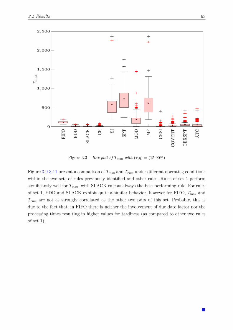
3.4 Results 63

FIF

O

EDD

SLACK

CR SI

SPT

MOD

MF

CRSI

COVERT

CEXSPT

ATC

0

500

1,000

1,500

2,000

2,500Tm

ax

Figure 3.3 – Box plot of Tmax with (τ,η) = (15,90%)

Figure 3.9-3.11 present a comparison of Tmax and Trms under different operating conditions

within the two sets of rules previously identified and other rules. Rules of set 1 perform

significantly well for Tmax, with SLACK rule as always the best performing rule. For rules

of set 1, EDD and SLACK exhibit quite a similar behavior, however for FIFO, Tmax and

Trms are not as strongly correlated as the other two pdrs of this set. Probably, this is

due to the fact that, in FIFO there is neither the involvement of due date factor nor the

processing times resulting in higher values for tardiness (as compared to other two rules

of set 1).

�


FIF

O

EDD

SLACK

CR SI

SPT

MOD

MF

CRSI

COVERT

CEXSPT

ATC

0

100

200

300

400

500

Tm

ax

Figure 3.4 – Box plot of Tmax with (τ,η) = (5,80%)

For stochastic models, it is required to construct a confidence interval for a parameter

estimate in statistical inferences. Bootstrapping procedure is used to obtain 95% confi-

dence intervals for the correlation coefficients between Tmax and Trms, which are presented

in Table 3.3. For SI rule, for example, under moderate load and tight due date condi-

tions, the confidence limits for the correlation coefficient is 0.814 (lower limit) and 0.918

(upper limit). Table 3.3 presents strong quantitative evidence that Tmax and Trms are

positively correlated. Moreover, this evidence does not require any strong assumptions

about the probability distribution of the correlation coefficient. It is also observed that

this correlation is stronger under High load and loose due date settings for all the rules.

The root mean square tardiness (Trms) is a very interesting measure as it permits to

differentiate a system with a little number of tardy jobs having higher values for tardiness

from a system with a lot of tardy jobs having low tardiness. It can also be used along with

mean tardiness to compute the variance of the tardiness. Moreover, it gives an indication

of the relative performance of the rules for Tmax as Trms is found to be strongly correlated

with the maximum tardiness.

�

3.4 Results 65

FIF

O

EDD

SLACK

CR SI

SPT

MOD

MF

CRSI

COVERT

CEXSPT

ATC

0

100

200

300

400

500Tm

ax


FIF

O

EDD

SLACK

CR SI

SPT

MOD

MF

CRSI

COVERT

CEXSPT

ATC

0

100

200

300

400

500

Tm

ax


�

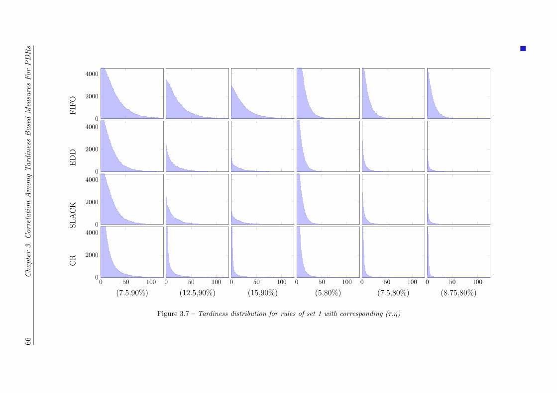
66Chapter

3.Correlation

Amon

gTardinessBased

MeasuresFor

PDRs

0

2000

4000

0

2000

4000

0

2000

4000

0 50 1000

2000

4000

0 50 100 0 50 100 0 50 100 0 50 100 0 50 100

FIFO

EDD

SLACK

CR

(7.5,90%) (12.5,90%) (15,90%) (5,80%) (7.5,80%) (8.75,80%)

Figure 3.7 – Tardiness distribution for rules of set 1 with corresponding (τ,η)

�

3.4Resu

lts67

0

2000

4000

0

2000

4000

0

2000

4000

0 50 1000

2000

4000

0 50 100 0 50 100 0 50 100 0 50 100 0 50 100

SI

SPT

MOD

MF

(7.5,90%) (12.5,90%) (15,90%) (5,80%) (7.5,80%) (8.75,80%)

Figure 3.8 – Tardiness distribution for rules of set 2 with corresponding (τ,η)

�


(7.5,90%) (12.5,90%) (15,90%) (5,90%) (7.5,90%) (8.75,90%)

40

60

80

100

120

140

160

180

200

220

Tmax

FIFOEDD

SLACKCR

(7.5,90%) (12.5,90%) (15,90%) (5,90%) (7.5,90%) (8.75,90%)

0

100

200

300

400

500

600

700

Trms

FIFOEDD

SLACKCR

(a) Tmax

(b) Trms

Figure 3.9 – Comparison of Tmax and Trms for rules of set 1

�

3.4 Results 69

(7.5,90%) (12.5,90%) (15,90%) (5,90%) (7.5,90%) (8.75,90%)

200

400

600

800

1,000

1,200

1,400

1,600

1,800

2,000

Tmax

SISPTMODMF

(7.5,90%) (12.5,90%) (15,90%) (5,90%) (7.5,90%) (8.75,90%)

0

500

1,000

1,500

2,000

Trms

SISPTMODMF

(a) Tmax

(b) Trms

Figure 3.10 – Comparison of Tmax and Trms for rules of set 2

�


(7.5,90%) (12.5,90%) (15,90%) (5,90%) (7.5,90%) (8.75,90%)

200

400

600

800

1,000

1,200

1,400

1,600

Tmax

CRSICOVERTCEXSPTATC

(7.5,90%) (12.5,90%) (15,90%) (5,90%) (7.5,90%) (8.75,90%)

0

50

100

150

200

250

300

350

Trms

CRSICOVERTCEXSPTATC

(a) Tmax

(b) Trms

Figure 3.11 – Comparison of Tmax and Trms for other rules

�

3.4 Results 71

Table 3.3 – Confidence Interval for Correlation between Tmax and Trms

(7.5,90%) (12.5,90%) (15,90%) (5,80%) (7.5,80%) (8.75,80%)

FIFO0.85529 0.85963 0.85604 0.74663 0.75248 0.75248

[0.7926,0.89986] [0.79261,0.90482] [0.78931,0.90291] [0.64096,0.84518] [0.64177,0.86386] [0.64177,0.86386]

SI0.89076 0.90969 0.91798 0.82116 0.85957 0.85957

[0.81299,0.94655] [0.84568,0.95843] [0.85023,0.96146] [0.73265,0.89054] [0.7919,0.91477] [0.7919,0.91477]

SPT0.87495 0.88438 0.88884 0.77426 0.80669 0.80669

[0.81709,0.91214] [0.83268,0.91846] [0.84133,0.92192] [0.68927,0.83444] [0.73219,0.86285] [0.73219,0.86285]

EDD0.87681 0.91346 0.89915 0.82829 0.88431 0.88431

[0.80323,0.92411] [0.87314,0.93581] [0.85284,0.92789] [0.73672,0.89456] [0.84067,0.91658] [0.84067,0.91658]

SLACK0.87442 0.92353 0.9143 0.82894 0.92511 0.92511

[0.80542,0.91772] [0.89158,0.9479] [0.88377,0.94044] [0.74006,0.89895] [0.89416,0.94954] [0.89416,0.94954]

CR0.88691 0.94371 0.94926 0.80228 0.92711 0.92711

[0.81835,0.92796] [0.91115,0.96202] [0.91001,0.96929] [0.71576,0.86626] [0.88473,0.959] [0.88473,0.959]

CR/SI0.92886 0.95837 0.98692 0.87255 0.95654 0.95654

[0.88921,0.96166] [0.91968,0.97568] [0.96101,0.99877] [0.80903,0.91708] [0.93018,0.97198] [0.93018,0.97198]

CoverT0.91365 0.9529 0.93416 0.85643 0.90983 0.90983

[0.8615,0.94638] [0.92114,0.97366] [0.88398,0.97113] [0.77751,0.91454] [0.83947,0.95133] [0.83947,0.95133]

MOD0.88924 0.93424 0.95677 0.86473 0.89796 0.89796

[0.83239,0.93016] [0.89132,0.96964] [0.93001,0.96886] [0.80519,0.90954] [0.85873,0.92713] [0.85873,0.92713]

CEXSPT0.92407 0.95033 0.95927 0.83688 0.90615 0.90615

[0.88205,0.96247] [0.90848,0.97623] [0.91218,0.98616] [0.7736,0.88755] [0.8533,0.93747] [0.8533,0.93747]

ATC0.92855 0.95065 0.9859 0.8715 0.94496 0.94496

[0.89352,0.95382] [0.91384,0.96863] [0.9693,0.99507] [0.81272,0.91484] [0.91124,0.96844] [0.91124,0.96844]

MF0.9091 0.92447 0.925 0.80034 0.83919 0.83919

[0.84872,0.95256] [0.86551,0.96275] [0.86443,0.96358] [0.70001,0.87661] [0.75322,0.90042] [0.75322,0.90042]

�


3.5 Conclusions

In this chapter, we have discussed tardiness based performance measures using a set of pdrs

that are extensively used in the literature on scheduling. From their relative performance

for the maximum tardiness, two sets of rules have been identified, FIFO, EDD, SLACK

and CR from one side and SI, SPT, MOD and MF on the other side. The behavior for the

rules of the first set is to exhibit a large number of tardy jobs with low tardiness, which

is exactly opposite to that for the rules of the second set. There are some rules (CRSI,

COVERT, CEXSPT and ATC) exhibiting these two behaviors under different conditions.

For tight due date setting, these rules behave more like the rules of set 1 while under loose

due date setting, their behavior tends towards rules of set 2. This kind of discrimination

is typically found through the Trms.

We found results that show a strong correlation between the Tmax and the Trms for a set

of pdrs that are extensively used in literature on scheduling. This correlation is found

to be relatively stronger in congested shops. The worst case performance in regards with

tardiness of a particular priority dispatching rule may therefore be predicted by evaluation

of Trms which can be used along with the mean tardiness to compute the variance of the

tardiness. So, the Trms can be used to rank the priority dispatching rules in regards with

the Tmax and the width of the tardiness.

�

4Learning based

Approach in Scheduling:

A Review

4.1 Introduction . . . . . . . . . . . . . . . . . . . . . . . . . . . . 73

4.2 A General Overview of Literature on Learning Based Scheduling 74

4.3 Literature Review on Inductive Learning in Scheduling . . . . 75

4.4 Parameters Influencing the Induction Algorithm . . . . . . . . 80

4.4.1 Feature Extraction and Selection . . . . . . . . . . . . . . . . . . . . . . 80

4.4.2 Discretization . . . . . . . . . . . . . . . . . . . . . . . . . . . . . . . . . 81

4.5 Conclusions . . . . . . . . . . . . . . . . . . . . . . . . . . . . . 81

This chapter gives a state-of-the-art survey on the use of learning based approaches in

the field of job shop scheduling. It provides an effective overview of the challenges and

benefits related to the application of learning algorithms in solving scheduling problems.

The survey reveals that their is a lack of systematic use of the scheduling knowledge

despite the fact that the approach has been acknowledged by most of the authors as

promising in scheduling domain. Moreover, it is generally not obvious how much a certain

set of scheduling data is relevant to the scheduling environment for desired objectives.

The emergence of data mining has invoked the academic interest in analyzing the complex

problems like this in a more methodical way.

4.1 Introduction

Scheduling is an important and complex activity in manufacturing that quickly crosses

the human cognitive capabilities even by a slight increase in its size. Machine learning

Part of this chapter was presented in the 8th International Conference of Modeling and Simula-tion (MOSIM’10) (Shahzad and Mebarki, 2010) (has been pre-selected for publication in EngineeringApplication of Artificial Intelligence, ISSN: 0952-1976, Imprint: ELSEVIER).

74 Chapter 4. Learning based Approach in Scheduling: A Review

simulates the human learning to assist in analyzing complex problems like scheduling.

Data mining integrates machine learning and modern database managements systems for

the discovery of new knowledge.

In recent years, several studies have focused on use of data mining as one of the approach

to understand the scheduling activities in a manufacturing system.

This chapter reviews the literature on the application of inductive learning algorithms and

their relative merits in the field of scheduling. The aim is to discuss the major contributions

in solving the scheduling problems and to identify their strengths and weaknesses. Case-

based reasoning, neural networks and inductive learning are the main approaches that

have been adapted to the scheduling problems.

Inductive learning approaches are considered to be more intuitive and hence gained much

attraction. Learning algorithms are greatly influenced by a number of parameters including

feature extraction, feature selection and discretization. Feature extraction involves the

creation of new attributes through transformation or combination of the primitive features.

Feature selection is the task of finding the most relevant subset of features for a classifier

to seek fewer features and maximum class separability.

The remainder of this chapter is organized as follows. We present a general overview of

literature on learning algorithms used in scheduling in § 4.2. A survey of the publications

applying inductive learning methods to scheduling problems is given in § 4.3. A brief

review of discretization, binning methods and feature selection is presented in § 4.4. In

the last section, some concluding remarks on this review are presented.

4.2 A General Overview of Literature on Learning

Based Scheduling

As there does not exist a pdr that is globally better than all the others (Lee et al., 1997),

numerous techniques based on the approach for dynamic selection of pdrs at the right mo-

ment according to the systems’ conditions and production objectives were proposed. This

approach is referred as multi-pass adaptive scheduling (MPAS) approach (Shiue and Guh,

2006a). Priore et al. (2001) categorized MPAS strategies as look-ahead simulation based

and knowledge based.

In the simulation based approach, the rule is chosen at the right moment by simu-

lating a set of pre-established dispatching rules and selecting the one that gives the

�

4.3 Literature Review on Inductive Learning in Scheduling 75

best performance (see for example, (Wu Richard and David, 1988; Wu and Wysk, 1989;

Ishii and Talavage, 1991; Yeong-Dae, 1994; Pierreval and Mebarki, 1997; Jeong and Kim,

1998)). The selected pdr is then used for a scheduling period of shorter length that may

be fix or dynamically sized according to system performance.

The second approach, from the field of artificial intelligence, employs a set of earlier sys-

tem simulations (training examples) to determine what the best rule is for each possible

system state. These training examples are used to train a machine-learning algorithm to

acquire knowledge about the manufacturing system (Michalski et al., 1986, 1998). Intel-

ligent decisions are then made in real time, based on this knowledge (see for example,

(Nakasuka and Yoshida, 1992; Shaw et al., 1992; Yeong-Dae, 1994; Min and Yih, 2003)).

The main algorithm types from the field of machine learning used in scheduling problems

include case-based reasoning (CBR), neural networks and inductive learning (Priore et al.,

2006). CBR is a kind of analogy-making that exploits the experience gained from the si-

milar problem-solving cases of the past (Watson, 1995). Lamatsch et al. (1988) employed

the same principle and incorporated reduction digraphs to search for a matching pro-

blem. Schmidt (1998) merged case-based reasoning with the theory of scheduling to solve

production planning and control problems using an interactive problem-solving frame-

work. However, due to extremely complex nature of scheduling problems, this approach

is considered inadequate (Aytug et al., 1994).

Inductive learning is broadly categorized as unsupervised and supervised inductive lear-

ning. In an unsupervised inductive learning, the learner is given only unlabeled examples,

the observations and it seeks to determine how the data is organized. On the other hand,

supervised learning is the machine learning task of inferring a function from supervised

training data. The training data consists of a set of training examples. Each example is a

pair consisting of an input object (typically a vector) and a desired output value. A su-

pervised learning algorithm analyzes the training data and produces an inferred function,

which is called a classifier. The next section gives a state-of-the-art on the use of inductive

learning in production scheduling.

4.3 Literature Review on Inductive Learning in Sche-

duling

Inductive learning in production scheduling has primarily been devoted to issues such as

selecting the best dispatching rule using simulation data. (Aytug et al., 1994) presented a

�


comprehensive review of different machine learning techniques with emphasis on inductive

learning methods applied in scheduling.

Pierreval and Ralambondrainy (1988) used the induction algorithm GENREG proposed

by (Ralambondrainy, 1988) to obtain a set of rules with best mean tardiness as target

concept on simulation data for flow shop environment. They acknowledged that the iden-

tified rules may not be strong enough, however it is mentioned that the approach is a

promising one especially when there is a lack of knowledge of the problem domain.

Nakasuka and Yoshida (1989) employed a learning algorithm named as Learning Aided

Dynamic Scheduler (LADS), capable of automatically generating new useful attributes for

on-line rule selection in a production line. The algorithm can handle quantitative as well as

qualitative type attributes. Selection of useful attributes is done using a local knowledge-

base (of each machine). They concluded that the good switching of rules can effectively

draw strong features of each individual rule. They also observed that incorporating a

mechanism to identify more informative problem sets increases the learning efficiency.

Shaw et al. (1992) developed pattern-directed scheduler (PDS) to monitor the scheduling

activity for changes in manufacturing patterns (combinations of various parameters that

together represent a given state of the system). Their system performed better than the

best dispatching rule considered for mean tardiness, under similar conditions. However

for higher number of machines and lower switching frequency of the selected rules, the

performance of system degraded.

Piramuthu et al. (1994) proposed a mechanism based on same principle to select among

a given set of heuristics using a well-known data mining algorithm C4.5, proposed by

(Quinlan, 2003) for decision tree generation for a flow shop. They considered both the

dispatching at individual machines and releasing jobs into the system. They investigated

the performance of PDS over a range of values for coefficient of variation of process

time and identified that their results were superior for large process time variations at

bottleneck machines. They observed that pattern-directed scheduling based decision trees

were not able to significantly improve upon the results. Moreover, these results are not

generalized.

Priore et al. (2001) used induction learning to select a heuristic through a set of training

examples created by using different values of the control attributes and identifying the

relevant manufacturing patterns. They observed that on certain occasions, the obtained

heuristic was bettered by the SPT or the EDD rule. A major cause of such behavior

is identified as the transitory changes of the control attributes. This effect is reduced by

assigning a weight function to each selected rule and triggering a rule only when its weight

�


reaches a certain lower limit.

Later, (Priore et al., 2006) compared inductive learning based on C4.5 algorithm with

other machine learning techniques for a selected flexible manufacturing system. They

incorporated a generator module to create new control attributes in order to reduce the

test error rate.

Li and Olafsson (2005) used decision-tree induction in their proposed approach to discover

the key scheduling concepts by applying data mining techniques on historic scheduling

data and to generate scheduling rules. Instead of selecting a particular pdr, they used the

dominance between two jobs (which job should be dispatched first) as the target concept

to be learned. This knowledge is then transformed in a form of dispatching lists. They

studied a single machine problem with Cmax as scheduling objective and compared the

performance with standard benchmark pdrs. They, however did not perform any selection

of the subset of data to be used for learning.

The review of the literature on knowledge based approach for MPAS reveals that the

usual practice involves the implementation of a pre-defined set consisting of a number of

candidate rules in a discrete event simulation model of the system under consideration,

and comparing their performance using simulation experiments under varying values of

system parameters characterizing the system dynamics. A set of best performing rules

under varying conditions are taken as training examples to be input to the learning sys-

tem. Intelligent decisions are then made in real time based on the knowledge obtained

through the learning system. Generally, examination of the simulation results suggests

changes to the selected rule-set, requiring repetition of at least a subset of the simula-

tion experiments. This, of course, assumes that all the dispatching rules are known in

advance and that the performance of these rules can accurately be simulated. Exception

to this usual approach include (Koonce and Tsai, 2000; Geiger et al., 2006; Huyet, 2006).

In most of these studies, simulation is not used for the generation of knowledge (although

it is employed in intermediate steps).

Lee et al. (1997) proposed to combine the strengths of genetic algorithm and induction

learning for developing a job shop scheduling system. Genetic algorithm used the heuristic

space as the search space. However they limited the learning process only to job release,

referring the difficulties to develop dispatching knowledge-bases for the dispatching phase.

Koonce and Tsai (2000) applied data mining on solutions generated by a genetic algorithm

(GA) based scheduling and developed a rule set approximating the GA scheduler. The

Attribute Oriented Induction approach was used to characterize the relationship between

the operations’ sequences and their attributes. The approach outperformed SPT, however

�


the obtained rules were unable to match the performance of GA scheduler.

Dimopoulos and Zalzala (2001) used genetic programming (GP) to evolve sequencing poli-

cies that combine known sequencing rules and problem specific information. They studied

a single machine scheduling problem with the objective of minimizing the total tardiness.

Various sets of problems are used for training the proposed GP-based algorithm for the

evolution of a dispatching rule. Nine dispatching rules were evolved with comparable per-

formance to man-made dispatching rules on training and validation problem set. However

the approach lacks transparency for a human scheduler in making decisions.

Ho and Tay (2005) made use of genetic programming as well for evolving effective compo-

site dispatching rules for solving a flexible JSSP with recirculation, with the objective of

minimizing total tardiness. They generated five pdrs for variable due date settings that are

reported to perform marginally well over the EDD in 74% to 85% of problem instances.

Their framework had the same drawback of lack of transparency as well as redundancy

of parameters in the evolved rules.

Geiger et al. (2006) proposed a genetic programming based system, named SCRUPLES

that combines an evolutionary learning mechanism with a simulation model to discover

new priority dispatching rules. They studied single machine scheduling problem with

three different objectives of minimizing∑

Ci, Lmax and∑

Ti. A framework for more

complex scheduling environments is also presented. They observed that number of jobs to

be scheduled has no significant impact on the performance of the system

Huyet and Paris (2004) proposed a methodology based on synergistic action of evolutio-

nary optimization and induction graph learning method to search for relevant knowledge

of manufacturing system. Optimization process provides increasingly efficient solutions

during its search. These solutions are then classified by the learning process using cer-

tain solution characteristics. These characteristics are highlighted in the learning process

to characterize the attractive areas of search space as well. They experimented with an

assembly kanban system for its optimal configuration.

Later, (Huyet, 2006) implemented the same approach for configuration of a job shop and

compared the results with a classical evolutionary optimization via simulation approach.

They generated some profiles for the system that contribute to characterization of high-

performance solutions.

As is evident from the prior work, the major contribution of learning in production sche-

duling is focused on selection of the best dispatching rule for specific conditions. Different

learning algorithms are used to extract the desired knowledge, with no algorithm capable

�


of outperforming others for all system conditions. The major drawback has been to ignore

the question of relevance of the solutions considered for the knowledge generation. The

contents of the scheduling knowledge play a major role in improving the efficiency of the

learning algorithm. However, it is generally not obvious which solutions would be more

relevant with respect to defined scheduling objectives in a particular environment. Simu-

lated data, historical data or data generated by some meta-heuristic like GA remained

the source of this scheduling knowledge. Huyet and Paris (2004) considered the problem

of relevance of scheduling knowledge while using GA to generate it.

A few studies focused on discovering new rules using GP and data mining. The proposed

approach relies on the solutions generated by tabu search. However instead of restricting

the focus on the pdr-space, dominance relations of competing jobs is identified, making use

of a set of pre-defined attributes. This differs from the selection of a pdr, where a selected

pdr is known to exist in the pool of candidate rules and is then used for dispatching jobs

during a certain length of scheduling period.

�


4.4 Parameters Influencing the Induction Algorithm

4.4.1 Feature Extraction and Selection

Feature extraction involves the creation of new attributes through transformation or

combination of the primitive features. Some of the important observations drawn

from literature review (Kwak and Yih, 2004; Metan et al., 2010; Zhao and Liu, 2007;

Siedlecki and Sklansky, 1993; Chen and Yih, 1996) are as under:

1. higher number of features is not necessarily beneficial for performance improvement.

2. Transformations or combinations of primitive features do not always guarantee bet-

ter performance.

3. Each attribute must consider some important information about the system under

consideration.

4. Attribute values must be computable at the right time with available information

at that time.

5. Generally, there exist feature interaction for a given subset of features, i.e. a feature

is not directly relevant to the target concept, rather it forms another feature subset

that is correlated to the target concept.

High dimensionality poses a challenge to learning tasks. Due to irrelevant features, clas-

sification algorithms tend to over-fit training data and degrade the generalization ability

(Guyon and Elisseefi, 2003; Shiue and Guh, 2006b). Feature selection is the task of finding

the most relevant subset of features for a classifier to seek fewer features and maximum

class separability (Kwak and Yih, 2004).The relevant features are those that are predictive

of the class whereas redundant features are those that are although predictive of the class

but are highly correlated with other predictive features (see (John et al., 1994) for de-

tails). Feature selection is an important issue in classification problems that leads to more

accurate and parsimonious models making it necessary to carefully examine the effect of

each attribute individually and combined with others (Chiu and Yih, 1995; Chen and Yih,

1996).

The two major approaches in feature selection are the filter and wrapper approaches

(John et al., 1994). The filter approach selects features independent of the objective func-

tion of the problem and ignores the effects of selected features on the performance of the

objective function (Kwak and Yih, 2004). The wrapper approach takes into account the

�

4.5 Conclusions 81

eventual objective function in its feature selection, however this approach may not be

computationally feasible with a large number of features (Hen et al., 2002).

4.4.2 Discretization

Some attributes may contain so many values that the mining algorithm cannot easily

identify interesting patterns in the data, from which to create a model. In these cases, one

can discretize such data to enable the use of the algorithms to develop a mining model.

Discretization is the process of dividing a scale variable into a small number of intervals,

or bins, where each bin is mapped to a separate category of the discretized variable.

The discretization process can significantly influence the effectiveness of a classification al-

gorithm, however it is virtually ignored in the machine learning literature (Kerber, 1992).

There is an extensive amount of literature on the discretization, however most of the

algorithms are static in nature, not taking into account the actual values. The interval

boundaries, hence may occur in the places that do not facilitate the accurate classifi-

cation. The simplest of these methods include equal-width-interval and equal-frequency-

intervals. Some more involved discretization methods include 1R algorithm (Holte, 1993),

ChiMerge (Kerber, 1992), StatDisc (Richeldi and Rossotto, 1995), Minimum Description

length principle Cut (MDLPC) (Fayyad and Irani, 1993), CONTRAST (van De Merckt,

1993) and FUSINTER (Rabaseda, 1996). Dougherty et al. (1995) provides an excellent

review of these discretization methods.

4.5 Conclusions

In this chapter, an overview of application of different approaches from the field of machine

learning in scheduling is presented with an emphasis on the inductive learning method.

Generally, in MPAS strategies employing machine learning, the performance of a set of

pre-defined pdrs on given objective function(s) is obtained through simulation. Best per-

forming pdrs under different conditions are selected as training examples for the learning

algorithm. The selection of training examples, in this case, is merely based on the perfor-

mance of a pdr relative to the set of pdrs simulated .

Case Based Reasoning (CBR), Artificial Neural Networks (ANN) and Inductive learning

are the main techniques among others, that are used for scheduling . CBR and its variants

�


are found to be inadequate due to very complex nature of scheduling problems and its

inability of generalization. ANN (especially Hopefield networks) require excessive com-

putation times despite their inherent parallelism. GA based schemes also suffer from the

problem of relevance and generality. The genetic programming (GP) based approaches

are found to be extremely sensitive to the selection of parameters and lacking the trans-

parency.

Decision Tree (DT) based inductive learning , on the other hand, is relatively simple yet

powerful technique capable of producing good results without compromising the transpa-

rency in decision-making process.

�

4.5Con

clusion

s83

Table 4.1 – Review of Literature

Reference Approach Learning PerformanceMeasures

Features Discretization Application

Pierreval and Ralambondrainy (1988) Simulation/Learning GENREG T 9 - Simplified FlowShop

Nakasuka and Yoshida (1989) Simulation/Learning LADS Cmax,ΣjTj 13 No FMS with transportation

Piramuthu et al. (1994) Simulation/Learning C4.5, PDS F 5 No Flow shop with machinefailure

Priore et al. (2001) Simulation/Learning InductiveLearning

T 4 Flow shop, Job shop

Priore et al. (2006) Simulation/Learning C4.5,BPNN,CBR T , F 7 No FMS with transportation

Metan et al. (2010) Simulation/DataMining

C4.5 T 26 No Job Shop

Lee et al. (1997) GA/Learning C4.5 ΣjTj 4 No Job shop

Koonce and Tsai (2000) GA/Data Mining AttributeOrientedInduction

Tmax 4 No Job shop

Dimopoulos and Zalzala (2001) GP ΣjTj 5 No Single Machine

Harrath et al. (2002) GA/Data Mining C4.5 5 Yes Job Shop

Kwak and Yih (2004) Simulation/DataMining

C4.5 ΣUj 11 No FMS

Huyet and Paris (2004) GA/Learning C4.5 JIT 22 No Job shop

Ho and Tay (2005) GP 7 No Job Shop

Li and Olafsson (2005) Simulation/DataMining

C4.5 Cmax 4 Yes Single Machine

Geiger et al. (2006) GP ΣjCj,Lmax,ΣjTj

17 No Single Machine, Flowshop.

Huyet (2006) GA/Learning C4.5 JIT 22 No Job shop

Shiue and Guh (2006a) GA/Learning ANN/C4.5 F ,ΣUj 30 No FMS

�

5Discovering Dispatching

Rules For JSSP through

Data Mining

5.1 Introduction . . . . . . . . . . . . . . . . . . . . . . . . . . . . 86

5.2 Background . . . . . . . . . . . . . . . . . . . . . . . . . . . . . 86

5.2.1 Tabu Search . . . . . . . . . . . . . . . . . . . . . . . . . . . . . . . . . 87

5.2.2 Data Mining . . . . . . . . . . . . . . . . . . . . . . . . . . . . . . . . . 88

5.3 Proposed Approach . . . . . . . . . . . . . . . . . . . . . . . . 88

5.3.1 Optimization Module . . . . . . . . . . . . . . . . . . . . . . . . . . . . 90

5.3.2 Simulation Module . . . . . . . . . . . . . . . . . . . . . . . . . . . . . . 91

5.3.3 Learning Module . . . . . . . . . . . . . . . . . . . . . . . . . . . . . . . 93

5.3.4 Control Module . . . . . . . . . . . . . . . . . . . . . . . . . . . . . . . . 95

5.3.5 Example . . . . . . . . . . . . . . . . . . . . . . . . . . . . . . . . . . . . 95

5.4 Experiments . . . . . . . . . . . . . . . . . . . . . . . . . . . . 98

5.4.1 System Attributes . . . . . . . . . . . . . . . . . . . . . . . . . . . . . . 99

5.5 Results and Discussion . . . . . . . . . . . . . . . . . . . . . . . 100

5.5.1 Obtained Rule-sets . . . . . . . . . . . . . . . . . . . . . . . . . . . . . . 100

5.5.2 Performance Metrics . . . . . . . . . . . . . . . . . . . . . . . . . . . . . 101

5.5.3 Results for Mean Tardiness (T ) . . . . . . . . . . . . . . . . . . . . . . . 103

5.5.4 Results for Maximum Tardiness (Tmax) . . . . . . . . . . . . . . . . . . 103

5.6 Conclusions . . . . . . . . . . . . . . . . . . . . . . . . . . . . . 108

A data mining based approach to discover previously unknown priority dispatching rules

for job shop scheduling problem is presented in this chapter. This approach is based

upon seeking the knowledge that is assumed to be embedded in the efficient solutions

provided by the optimization module built using tabu search. The objective is to discover

the scheduling concepts using data mining and hence to obtain a set of rules capable of

approximating the efficient solutions for a job shop scheduling problem (JSSP). A data

mining based scheduling framework is presented and implemented for a job shop problem

Part of this chapter was presented in the 8th International Conference of Modeling and Simulation(MOSIM’10) (Shahzad and Mebarki, 2010) (has been pre-selected in Engineering Application of ArtificialIntelligence, ISSN: 0952-1976, Imprint: ELSEVIER).

86 Chapter 5. Discovering Dispatching Rules For JSSP through Data Mining

with mean tardiness and maximum lateness as the scheduling objectives. The results

indicate the superior performance of the proposed system relative to a number of priority

dispatching rules and hence proves to be promising approach.

5.1 Introduction

The major drawbacks of pdrs include their performance-dependence on the state of the

system and non-existence of any single rule, superior to all the others for all possible states

the system might be in (Geiger et al., 2006). Meta-heuristics (e.g., simulated annealing,

tabu search etc) have an advantage over pdrs in terms of solution quality and robustness,

however these are usually more difficult to implement and tune, and computationally too

complex to be used in a real time system.

Robust and better-quality solutions provided by meta-heuristics contain useful knowledge

about the problem domain and solution space explored. Such a set of solutions represents a

wealth of scheduling knowledge to the domain that can be transformed in a form of decision

tree or a rule-set. Here, we propose an approach to exploit this scheduling knowledge. In

our approach, we seek this scheduling knowledge through a data mining module to identify

a rule-set by exploring the patterns in the solution set obtained by an optimization module

based on tabu search, a very efficient meta-heuristic for JSSP in particular. This rule-set

approximates the output of the optimization module when incorporated in a simulation

model of the system. This rule-set is subsequently used to make dispatching decisions in

an on-line manner.

This chapter is organized as follows. A brief description of some necessary background

areas such as tabu search and data mining is given in § 5.2. The proposed framework is

presented in § 5.3 along with the details of the different modules. In § 5.4 , the design of

experiments for the proposed framework is given. The results and discussions are provided

in section § 5.5 . Conclusions and some perspectives of this study are presented in the last

section.

5.2 Background

Some background areas must be discussed before presenting the proposed framework.

These include Tabu search; one of the most effective metaheuristic to solve JSSP and

data mining; a knowledge discovery approach.

�

5.2 Background 87

5.2.1 Tabu Search

Tabu search (TS) algorithms are among the most effective approaches for solving JSSP

(Jain and Meeran, 1998) using a memory function to avoid being trapped in a local op-

timum (Zhang et al., 2008). Most state-of-the-art algorithms for JSSP include some sort

of tabu search functionality (Zobolas et al., 2008). However, neighborhood structures and

move evaluation strategies play the central role in the effectiveness and efficiency of the

tabu search for the JSSP (Jain et al., 2000). In contrast to myopic nature of PDRs, meta-

heuristics such as tabu search can attack the problem more rigorously and intelligently

due to relatively higher level of domain knowledge. As a consequence, the decisions made

by the proposed system reflect the use of this valuable knowledge.

The fundamental element underlying tabu search is the use of flexible memory that ac-

quires domain and search space relevant information and profits from it as well (Laguna,

1994). The basic tabu search procedure is quite simple. A feasible initial solution is used

as a starting point and is set as current seed and the best solution. Depending upon the

neighborhood structure, a finite number of neighbors of the current seed are found, that

represent the candidate solutions. Through the performance evaluation of those candidate

solutions that are are not tabu (one that is obtained through a forbidden move) or those

that do not satisfy aspiration criteria (to overrule the tabu status), the best one is selected

as the new current seed. This selection is called a move added to tabu list, while removing

the oldest move from this list. New seed solution assumes the place of current best, if it

is better than it. The procedure is iterated until the stop criterion is met.

A huge number of variations in this basic procedure of tabu search can be found in

literature. The most common variation include flexible tabu length, neighbor structure,

multi-start search, aspiration and stopping criteria etc. Neighborhood structure is the

most crucial ingredient of a particular tabu search algorithm. It is a mechanism to obtain a

new set of neighbors by applying small perturbations to the current solution (Zhang et al.,

2007).

Neighborhood structure is directly effective on the efficiency of TS algorithm (Jain et al.,

2000). A neighborhood structure is a mechanism which can obtain a new set of neighboring

solutions by applying small perturbations to a given solution. Each neighbor solution is

reached immediately from a given solution by a move.

The earliest implementations of tabu search in JSSP include (Taillard, 1994;

Dell’Amico and Trubian, 1993; Barnes and Chambers, 1995). The TSAB (Tabu Search

Algorithm with Back jump tracing) method Nowicki and Smutnicki (1996) however, in-

�


troduced a real breakthrough in terms of efficiency and effectiveness for the JSSP. The

i-TSAB technique proposed by Nowicki and Smutnicki (1996) improves upon the ear-

lier algorithm and represents the current-state-of the-art for JSSP. Later, (Watson et al.,

2005, 2006) analyzed the reasons of effectiveness of tabu search in JSSP. Some hybrid

methods are also proposed to further improve the efficiency. These include the work of

(Pezzella and Merelli, 2000), who combined tabu search with shifting bottleneck heuristic

and (Zhang et al., 2008) proposing a very effective hybrid tabu-search simulated annealing

method.

5.2.2 Data Mining

Data mining is an essential step in process of knowledge discovery from data (KDD),

however the two terms are often used interchangeably. Data mining is the process of

discovering interesting knowledge from large amounts of data stored in databases, data

warehouses, or other information repositories (Han and Kamber, 2002). The data mining

approach is particularly applicable for large, complex production environments, where the

complexity makes it difficult to model the system explicitly.

From the viewpoint of our approach, data mining can specifically be considered as the

analysis of a data set, referred as training data set in order to identify previously unknown

and potentially useful hidden patterns and to discover relationships among the various

elements of this data set. The aim is to classify the cases in another data set, referred as test

data set, by mapping the newly discovered relationships on them. The discovery process

can be termed as descriptive data mining, while the classification of test data set using

the discovered relationships can be viewed as predictive data mining (Choudhary et al.,

2009).

We use decision tree based learning as the data mining step as it is simple to understand

and interpret, requires little data preparation, able to handle both numerical and cate-

gorical data, uses a white box model, possible to validate a model using statistical tests,

robust and performs well with large data in a short time. Induction of decision tree, or ID3

(Iterative Dichotomiser 3) (Quinlan, 1986) is one of the most powerful mining algorithm

used in machine learning (Koonce and Tsai, 2000; Dudas et al., 2009; Priore et al., 2006).

Revised versions of ID3 include GID3 (Generalized ID3), ID4, ID5, C4.5 (Quinlan, 2003)

and C5.0 (Quinlan, 2003).

�

5.3 Proposed Approach 89

5.3 Proposed Approach

We propose a hybrid simulation-optimization based approach coupled with data mining

for job shop scheduling problem. The goal of the proposed system is to generate a set of

rules for making dispatching decisions in a job shop scheduling environment.

First of all control module generates number of problem instances relevant to real sche-

duling system. This may be replaced by historical data of the manufacturing system.

These problem instances are stored in an instance database. The optimization module

generates solutions for a subset of these instances. This subset of job shop instances is

referred as initial training data set. The solutions to these instances generated by an op-

timization module are in fact a set of good scheduling decisions that may be made for

the manufacturing system. However these good decisions are not evident before these are

implemented and corresponding performance measures have been computed. In order to

identify and extract the characteristics of these good scheduling decisions, a simulation

module is employed which associates a performance measure to each decision taken by

the optimization module. This refined set of characteristics of scheduling decisions refers

to a relevant scheduling knowledge. The scheduling knowledge is stored in a scheduling

database and employed by a learning process to construct a decision tree. This decision

tree is then used to dispatch the jobs-awaiting service in an on-line manner. The decision

tree is dynamically updated, whenever necessary through a control module. The control

module transmits the knowledge of good scheduling decisions to the optimization module

as well to improve its own performance at subsequent levels.

Figure 5.1 demonstrates the interaction of these modules in the proposed framework.

There are two important aspects of the proposed system besides merely providing a sche-

dule,

1. to provide an insight to the scheduling decisions made by the optimization module

and

2. to improve upon the efficiency of the optimization module by utilizing the output

of learning module.

Scheduling procedures such as pdrs and meta-heuristics do not provide, in general, any

justification of the decisions made, no matter how good or bad they are. This lack of

transparency is not only undesirable in practice but also a great hindrance to understand

the difference between good and bad scheduling decisions. Identifying the characteristics

�


of good scheduling decisions generated by an optimization process is thus desired. Our

proposed system is aimed at providing transparency in its scheduling decisions.

The proposed system takes benefit from this white-box effect, by making use of the relevant

scheduling knowledge in optimization process. The meta-heuristics such as tabu search

use a neighborhood mechanism to reduce the search space. Optimization process can make

use of this knowledge to create more restricted and potentially stronger neighborhoods.

Figure 5.1 – The proposed framework

In the following, the structural detail of each module as well as interaction of these modules

is explained.

5.3.1 Optimization Module

The optimization module is aimed at providing the most relevant solutions to the schedu-

ling problem. A tabu search, (Nowicki and Smutnicki, 1996) based optimization module

generates a set of efficient solutions for a set of problem instances. Since these efficient

solutions are obtained through a series of some logical moves of the meta-heuristic, they

�


have some general characteristics that may describe the relationship between operations

and their sequential order in a particular solution. These characteristics are a form of

schedule knowledge, like dispatching rules. The aggregation of corresponding set of effi-

cient solutions for each problem instance may then be used as the training data set for the

data mining algorithm for discovery of scheduling knowledge. However, it is not expected

from this module to identify a priori, the reasons of superiority of one solution to another.

The optimization module works in an off-line manner, however it continually provides

with more and more schedules to the problem instances generated by the control module.

5.3.2 Simulation Module

There are three key functions of the simulation module. Figure 5.2 shows the working of

simulation module. The main simulator that is in-loop with learning module, takes the

schedule generated by optimization module. This schedule is transformed into a set of

decisions, i.e. whether a job is dispatched before some other job. Each decision is charac-

terized by a vector of attribute-value pairs, where attributes are the selected attributes

and the values are obtained through this simulator. A collection of these vectors is referred

as a training block (Chong et al., 2004), (see § 5.3.2.1 ).

Finally, the simulator associates a relative performance measure to a decision made in

the schedule. This is done by considering some alternative decisions at each dispatching

decision point. These alternative decisions are taken from a multi-pass simulator, that

measures the performance of a pre-defined set of pdrs. Each time a dispatching decision

is made, it is compared with the best possible decision by the multi-pass simulator. Based

on this comparison, a relative value of performance is associated with the decision. In

this way, equivalent schedules are incorporated in the training data set. Both of these

simulators take on the same set of problem instances.

5.3.2.1 Training Block

A training block, Bi is a matrix of the form

Bi =

[

x z

]

�


σTSMain

Simulator

χx

x1x2

...xp

χ1 χ2 χ3 . . . χl z1x11 x12 x13 . . . x1l z11

x21 x22 x23 . . . x2l z12

......

......

xp1 xp2 xp3 . . . xpl z1p

pdrsMultipassSimulator

PerformanceMeasures

Figure 5.2 – Simulation Module

with

x =

[

x1 x2 x3 . . . xp

]T

and

z =

[

z1 z2 z3 . . . zq

]T

where p is the number of positive examples in a training block and q is the number of

objectives considered. Each row in x is composed of values of the selected attributes at

any instant, whereas each z represents the target concept to be learned. The minimum

training block is {x1,z1}T . Each element (x,z)∈ Bi represents an example from which we

can learn. We refer to each such example or a row in Bi as a positive training example.

Each xk is an l-dimensional row vector, i.e., ∃k,1 6 k 6 p,

xk =

[

xk1 xk2 xk3 . . . xkl

]

where l is the number of selected attributes with each attribute χ appearing as a column

vector in Bi.

For z = z1, z becomes a p-dimensional column vector, i.e.

[

z11 z21 z13 . . . z1p

]T

,∀k,zk ∈ {0,1}

zk (zk := precedesu,v,q) is a binary variable representing the processing order of two jobs

u, v on machine q, i.e. zk = 1 represents u → v and vice versa.

Each training block, Bi is a chronological sequence of consecutive x’s and corresponding

�


z’s, before another sequence of consecutive x’s follows. A union of these training blocks is

the training data set, B used by the learning module, and is expressed as

B =

[

B1 B2 B3 . . . Bn

]T

.

There is another simulation model, within the simulation module, that serves the purpose

of an observer to the manufacturing system. It records the performance of the system

in response to the scheduling decisions taken. This information is used by a controller

module for subsequent generation of training data. Since the actual scheduling decisions

are taken on the basis of dispatching list generated by learning module, the performance

of the system may differ significantly even for the same training data set.

5.3.3 Learning Module

As the solutions in the solution-set used by learning module are restricted to perform above

certain threshold, focus remains on the more relevant search space. Figure 5.3 illustrates

the working of learning module. The learning module takes the refined relevant scheduling

knowledge from the scheduling database. This knowledge constitutes the learning set on

which the induction process is built. This process aims at predicting a class of scheduling

decisions that may be most accurately generalized.

χ1 χ2 χ3 z1

v1 v5 v6 0

v3 v4 v6 0

v2 v5 v8 1

v1 v5 v8 0

v3 v5 v7 1

v3 v4 v6 0

v2 v4 v7 1

v3 v4 v8 0

χ1

0

v1

1

v2

{0,1}

0

v4

1

v5

v3

Figure 5.3 – An Example of Generating Decision Tree from a Simple Training Block

The learning module deciphers the scheduling data so as to make a particular decision

as transparent as possible. It is quite easy to understand the process of classification of

scheduling decisions when it is represented as a decision tree. This is the key advantage of

the decision tree based learning and the major reason to adopt this method in the proposed

�


framework. Learning module uses C4.5 algorithm for mining the implicit information in

the solutions found by optimization module.

The relevant scheduling knowledge is provided in the form of training blocks from the

scheduling database. The collection of these training blocks is used by the learning module

as initial training data. However, considerable amount of transformation is required before

it is possible to mine any useful knowledge from the data.

Construction of a proper training data set is a very crucial point in the entire Knowledge

Discovery from Data (KDD) process. From the data mining perspective in JSSP, the

target concept to be learned is to determine which job should be dispatched first within

a set of schedulable jobs on the same machine at a particular instant. Extracting this

knowledge from the training data set would allow us to dispatch the next job at any given

time and thereafter to create dispatching lists for any set of jobs.

Finally, the decision tree induced using the learning algorithm can be applied directly to

the same JSSP to validate the explored knowledge and as a predictive model to predict

the target concept. A set of scheduling problem instances with similar distribution of

processing time is to be used as a test data set for the scheduling knowledge discovered.

The overall sequence of operations obtained by these rules is translated to a schedule using

a schedule generator. Thus, the tree will, given any two jobs, predict which job should

be dispatched first and can be thought of as a new, previously unknown rule. In addition

to the prediction, decision trees and decision rules reveal insightful structural knowledge

that can be used to further enhance the scheduling decision.

The training blocks provide valuable information about the current status of the system.

It is the selection of proper attributes, that can provide with efficient training blocks

to help in generating a better quality decision tree. Attribute selection is the task of

finding the most reasonable subset of attributes for a classifier to seek fewer attributes

and maximum class separability (Kwak and Yih, 2004). This process is also critical for

the effectiveness of the subsequent model induction by eliminating certain redundant and

irrelevant attributes. It is indeed unlikely that the attributes that are recorded as part of

the available data are the attributes that are the most relevant or useful for data mining

process. Thus, creation of new attributes must be considered.

There exist a strong relation among the sequencing of operations due to precedence

constraints, however, considering only two (operations of the) jobs on the same machine

among schedulable jobs (the predecessor (if any) of whom are already dispatched) at any

instance for the comparison reduces this dependency effect. Proper selection of attributes

plays an important role to reduce this dependency as well.

�


Both the creation of new attributes and selection of attributes (we call the both process

combined as attribute extraction) are primarily linked with the objectives of the JSSP.

Tardiness based objectives require different attributes to be taken into account while flow-

time based objectives have different requirements. For instance, deadline related statistics

and counters are more suited for tardiness based objectives.

Arithmetic combinations of primitive attributes can also be used to generate new useful

attributes. However a large set of attributes is not desirable, as the attributes are generally

not independent of each other, making the process computationally impractical. Several

heuristics such as backward stepwise heuristic, forward stepwise group heuristic have been

proposed to limit the selected subset of attributes while maintaining a certain performance

level.

5.3.4 Control Module

A control module generates the relevant scheduling problem instances. These instances

may represent historical data of the manufacturing system. An on-line controller module

takes the relevant dispatching decisions from the dispatching database, to be implemented

in actual manufacturing system.

As a scheduling decision is implemented in a manufacturing system, an online performance

monitoring is done, to decide whether a new training block is generated for the recent de-

cisions or not. If the actual performance of the system degrades below a certain threshold,

controller triggers the learning process for the updating of dispatching database.

A control sub-module is employed for providing feed-back to the optimization module.

Feedback to optimization module serves the purpose of improving its own performance at

subsequent levels.

5.3.5 Example

In Table 5.1, an instance of a 6× 6 problem is given. This instance is taken from training

problem set and is solved by the tabu search for mean tardiness (T ). The solution provided

by Tabu Search (TS) is illustrated using disjunctive graph representation in Figure 5.4.

Corresponding to each disjunctive arc, we get as many examples to learn as there are

number of jobs at time t, waiting in the queue corresponding to the machine represented by

�


disjunctive arc. This forms a training block for this particular instance, to be incorporated

in training data set B.

For illustrative purpose, same instance is solved by RS for T and shown in Figure 5.4. It

is observed that only 14 out of 30 disjunctive arcs coincide in these two graphs, making

only 17 out of 36 operations to be processed on the same sequence. However, the earliest

non-coincident arc is the first arc on machine 4 (O34 → O64 in Figure 5.5). Fixing this

arc direction as given by TS and applying an active scheduler immediately gives the same

solution as given by TS. This is not true in general, however fixing the earlier arcs for a

solution provided by RS results in much closer or identical sequence to the one provided

by TS.

Table 5.1 – An Instance from the Test Data Set

J Mj,pj

J1 3,4 1,6 2,8 4,5 6,8 5,7 22

J2 6,4 2,1 1,10 3,1 4,2 5,3 26

J3 1,1 2,4 4,2 6,2 3,1 5,1 25

J4 1,6 2,3 4,9 3,8 5,9 6,8 23

J5 5,3 2,4 6,6 1,7 3,7 4,3 18

J6 1,4 2,1 4,2 3,10 5,4 6,5 28

O13 O114

O126

O148

O165

O158

O26 O224

O211

O2310

O241

O252

O31 O321

O344

O362

O332

O351

O41 O426

O443

O439

O458

O469

O55 O523

O564

O516

O537

O547

O61 O624

O641

O632

O6510

O660

O⋄⋄

00

0

00

0

O⋆⋆

73

1

8

35

Figure 5.4 – Disjunctive Graph Solution Given by Tabu Search

�


O13 O114

O126

O148

O165

O158

O26 O224

O211

O2310

O241

O252

O31 O321

O344

O362

O332

O351

O41 O426

O443

O439

O458

O469

O55 O523

O564

O516

O537

O547

O61 O624

O641

O632

O6510

O660

O⋄⋄

00

0

00

0

O⋆⋆

73

1

8

35

Figure 5.5 – Disjunctive Graph Solution Given by Rule Set

�


5.4 Experiments

Table 5.2 summarizes the experimental setup used. Two sets of 6 × 6 similarly sized

instances of a static job shop problem with different seed values are used as training

data-set I and test data-set I. All jobs are available simultaneously at time zero. Discrete

uniform distribution between 1 and 10 is used to generate the operation processing times.

The job due dates are determined using two parameters τ and ρ, where τ determines the

expected number of tardy jobs (and hence the average tightness of the due dates) and ρ

specifies the due date range. Once these parameters have been specified, the job due dates

are generated from the discrete uniform distribution given as

dj = UNIFORM(µ−µρ

2,µ+

µρ

2)

where µ = (1− τ)E[Cmax] is the mean due date. E[Cmax] denotes the expected makespan

for the problem instance and is calculated by estimating the total processing time required

by all operations divided by the number of machines. Note that this assumes no idle time

on machines, and hence will be an optimistic estimate of Cmax. We consider τ = 0.3 and

ρ = 0.5. T (Mean Tardiness ) and Tmax (Maximum Tardiness) are used as the scheduling

objectives.

Table 5.2 – Experimental Setup

Parameter Value

Data Sets Training Data-set (I), Test Data-set (I)

Problem size 6× 6

Number of training instances, ♯I 100

Number of test instances, ♯I 50

Release dates, rj 0

Operation processing times, pj(i) U[1,10]

Due-dtaes, dj UNIFORM(µ− µρ

2,µ+ µρ

2)

Objectives, f T , Tmax

�

5.4 Experiments 99

5.4.1 System Attributes

Selection of the relevant attributes has a key role in obtaining the appropriate perfor-

mance level from knowledge-based systems. The selected attributes have the following

characteristics:

– The attributes are related to tardiness based performance measures.

– It is preferred to define attributes in relative values instead of absolute values.

– The attributes with high variation are discretized.

Table 5.3 lists the attributes used in the experiments. The selection of these attributes is

based on earlier research (see for example, (Kwak and Yih, 2004; Cho and Wysk, 1993;

Chen and Yih, 1996)). However, it is acknowledged that a simple model is not capable to

generate and guarantee near-optimal subset of attributes. A more rigorous approach for

the combinatorial attribute selection may be used at the cost of extra computational com-

plexity(see (Siedlecki and Sklansky, 1989) for review and limitations of other approaches).

Table 5.3 – Selected Attributes for Tmax

ExpressionDescription

nt Number of jobs in the system at any instant t.

max − Difference between maximum and average remaining processing times.

np

ntPercentage of jobs with long processing times.

nd

ntPercentage of jobs with relatively loose due dates.

Average remaining processing time.

ς Average remaining time until due-dates.

ς

Relative tightness ratio.

E(f) Expected value of Tmax

Some of the attributes are system related, that are not specifically related to a prticular

job or a specif set of jobs. A few attributes are specific only to the jobs considered for the

comparison.

For static job shop problems, as we considered in this chapter, nt = n at rj for all jobs.

Higher the nt, greater is the size of training block and there are more and more examples

�


for that instance to learn the target concept.

∆ j, and max − uses the remaining processing time for direct comparison of two jobs,

as an average measure and relative value among all the jobs in system. It is important

to note that it is the combined effect of these attributes along-with others, that plays a

role in strengthening their relation with the target concept. For example, in relation

with nt and max − affects thenp

nt. Hence it is very difficult to identify a relationship

of an attribute with the target concept. The predicted value of the performance measure

is also used as an attribute, however it is again not independent from the other selected

attributes.

For this study, we used the binning method, which is an unsupervised discretization

method. Based on the values of the mean and standard deviation of the distribution of

the specified attribute(s), we generate a field with banded categories. Figure 5.6 illustrates

a ±3 standard deviation based discretization for an attribute to generate seven bins.

However, creating banded categories based on standard deviations may result in some

bins being defined outside the actual data range and even outside the range of possible

data values.

**

−42.4 −28.5 −14.5 13.4 27.3 43.2

Figure 5.6 – Standard Deviation based Discretization of for Lmax

5.5 Results and Discussion

5.5.1 Obtained Rule-sets

A set of 19 rules for the T and a set of 57 rules Tmax are generated by the proposed system

using 100 training blocks of different sizes from the similarly sized problem instances. The

differences in the size of the training blocks is due to the fact that the generated training

blocks are dependent on the machine precedence constraints of the problem instance as

well as the solution method. A partial list of the rules induced is given in Table 5.4 and

Table 5.5. The prediction accuracy of these rule sets for T and Tmax is found to be 79.52%

and 69.93% respectively.

�

5.5 Results and Discussion 101

Table 5.4 – A partial list of inferred rules for T

No. Rule

Rule 1 for 0 ∆ςj <= 1 ∧ Bin(∆pj)in[1] ∧∆ςj > −12 ⇒ 0

Rule 2 for 0 ∆ςj <= 1 ∧ Bin(∆pj)in[2] ⇒ 0

Rule 3 for 0 ∆ςj > 1 ∧ Bin(∆pj)in[−1] ∧∆ςj > 11 ⇒ 0

Rule 4 for 0 ∆ςj > 1 ∧ Bin(∆pj)in[0] ∧ Bin(∆ j)in[−2] ∧∆CRj = 0.469 ⇒ 0

Rule 5 for 0 ∆ςj > 1 ∧ Bin(∆pj)in[0] ∧ Bin(∆ j)in[−1] ∧ <= 31.333 ⇒ 0

Rule 6 for 0 ∆ςj > 1 ∧ Bin(∆pj)in[0] ∧ IRBin(∆pj)in[−1] ∧ > 31.333 ∧ <=218.800 ∧∆ςj > 8 ⇒ 0

Rule 7 for 0 ∆ςj > 1 ∧ Bin(∆pj)in[0] ∧ Bin(∆ j)in[−1] ∧ > 31.333 ∧ >218.800 ⇒ 0

Rule 8 for 0 ∆ςj > 1 ∧ Bin(∆pj)in[0] ∧ Bin(∆ j)in[0] ⇒ 0

Rule 9 for 0 ∆ςj > 1 ∧ Bin(∆pj)in[1 2] ⇒ 0

Rule 1 for 1 ∆ςj <= 1 ∧ Bin(∆pj)in[−2 − 1 0] ⇒ 1

Rule 2 for 1 ∆ςj <= 1 ∧ Bin(∆pj)in[1] ∧∆ςj <= −12 ⇒ 1

Rule 3 for 1 ∆ςj > 1 ∧ Bin(∆pj)in[−2] ⇒ 1

Rule 4 for 1 ∆ςj > 1 ∧ Bin(∆pj)in[−1] ∧∆ςj <= 11 ⇒ 1

Rule 5 for 1 ∆ςj > 1 ∧ Bin(∆pj)in[0] ∧ Bin(∆ j)in[−3] ⇒ 1

Rule 6 for 1 ∆ςj > 1 ∧ Bin(∆pj)in[0] ∧ Bin(∆ j)in[−2] ∧∆CRj0.469 ⇒ 1

Rule 7 for 1 ∆ςj > 1 ∧ Bin(∆pj)in[0] ∧ Bin(∆ j)in[−1] ∧ > 31.333 ∧ <=218.800 ∧∆ςj <= 8 ⇒ 1

5.5.2 Performance Metrics

Performance of the proposed system is measured in relative terms and is indicated by two

measures namely ηf1 and ηf2 . η1 indicates performance of obtained rule-set and the set of

pdrs relative to solution provided by tabu search on the objective function f for set of

training problem instances (I). Average value of ηf1 over I is given as,

ηf1 =

f(r,I)−f(TS,I)f(TS,I)

if f(r,I) > 0

0 otherwise

where

r ∈ {FIFO,SI,SPT,EDD,SLACK,CR,

CR/SI,COV ERT,CEXSPT,ATC,MF}

, TS: Tabu Search, RS: Rule-Set obtained and I: set of training problem instances used.

For example, Tmax(r,I) represents the set of Tmax values for all the problem instances of

�


Table 5.5 – A partial list of inferred rules for Tmax

No. Rule

Rule 1 for 0 E(Tmax) 6 0 ∧ 6 126.200 ∧ > 102.400 ⇒ 0

Rule 2 for 0 E(Tmax) 6 0 ∧ 6 126.200 ∧ > 102.400 ∧ pmax−

pmax> 13.560 ∧

np

nt6

0.500 ⇒ 0

Rule 3 for 0 E(Tmax) > 0 ∧np

nt6 0.200 ∧ ς 6 −25 ∧ 6 1379.200 ∧ pmax−

pmax6

−231.360 ⇒ 0


nt6 0.200 ∧ ς 6 −25 ∧ 6 1379.200 ∧ pmax−

pmax>

−231.360 ∧ pmax−

pmax6 −213.600 ∧ ς 6 −29 ∧ > 1351.200 ⇒ 0


nt6 0.200 ∧ ς 6 −25 ∧ 6 1379.200 ∧ pmax−

pmax>

−231.360 ∧ pmax−

pmax6 −213.600 ∧ ς > −29 ∧ E(Tmax) > 91 ⇒ 0


pmax6 13.560 ⇒ 1


pmax> 13.560 ∧

np

nt>

0.500 ⇒ 1

Rule 3 for 1 E(Tmax) 6 0 ∧ > 126.200 ⇒ 1


nt6 0.200 ∧ ς 6 −25 ∧ 6 1379.200 ∧ pmax−

pmax>

−231.360 ∧ pmax−

pmax6 −213.600 ∧ ς 6 −29 ∧ 6 1351.200 ⇒ 1


nt6 0.200 ∧ ς 6 −25 ∧ 6 1379.200 ∧ pmax−

pmax>

−231.360 ∧ pmax−

pmax6 −213.600 ∧ ς > −29 ∧ E(Tmax) <= 91 ⇒ 1

training set I using the set of pdrs in set r.

Note that ηf1 is an indication of the average performance of TS algorithm relative to pdrs.

On the other hand, ηf2 refers to the performance of obtained rule-set relative to considered

set of pdrs and is given as,

ηf2 =

f(r,I)−f(RS,I)

f(RS,I)if f(r,I) > 0

0 otherwise

Lower value of ηf1 for a pdr given for any problem instance means that solution by that

pdr is close to the one provided by TS algorithm. In this case, the performance of the

system relative to pdr (given by ηf2 ) appears to be degraded however, the fact is that its

performance is close to the optimum reached by TS. Consequently, a lower value of ηf2 is

observed for that instance despite of obtaining a good schedule. This negatively affects on

the average performance. This means that instances with higher value for ηf1 for the pdrs

are more representative of the real performance of the proposed system. Higher value for

ηf2 , in this case, indicates good performance of the system relative to pdrs and vice versa.

�


5.5.3 Results for Mean Tardiness (T )

Figure 5.7(a) and Figure 5.7(b) show the plots for ηT1 and ηT2 respectively. For T , the RS

performs well over all pdrs with SI as the second best performer. However, the SLACK

rule is the worst performer for this objective. Figure 5.8 presents the boxplot providing a

comparative overview of the T values across the test instances. This graphic provides the

distribution of actual values of T for all pdrs, RS and TS.

For the comparison of performance on individual instances, we found that out of 50 test

instances, for only 28 instances, the RS provided better solutions than any other pdr with

best solution among pdrs for that instance. On the average, these better solutions were

found to be 14% more efficient than the best solution by the best pdrs on those instance.

However the computational time to solve all test instances is relatively higher for RS,

assuming the time required for each pdr to be the same.

5.5.4 Results for Maximum Tardiness (Tmax)

In Figure 5.9(a) and Figure 5.9(b) the plots for ηTmax1 and ηTmax

2 are presented respectively.

It is observed that the results of mined rule-set are superior to the pdrs for the Tmax

measure.

For a set of fifty test instances, plot of η2, shown in Figure 5.9(b), reflects the fact that the

rule-set is consistently a better performer among all the pdrs used with slack rule as the

closest competitor. This is due to the nature of selected attributes used in the algorithm.

There is a considerable room of improvement in performance of rule-set, as can be seen

from plot of η1 shown in Figure 5.9(a), that may be obtained through better attribute

selection. Figure 5.10 presents the box-plot providing a comparative overview of the Tmax

values across the test instances, providing the distribution of Tmax for all pdrs, RS and

TS.

�


FIFO SI SPT EDD SLACK CR CRSI COVERT MOD CEXSPT ATC MF RS

0

5 · 10−2

0.1

0.15

0.2

0.25

0.3

0.35

ηT 1

FIFO SI SPT EDD SLACK CR CRSI COVERT MOD CEXSPT ATC MF

0

2 · 10−2

4 · 10−2

6 · 10−2

8 · 10−2

0.1

0.12

0.14

0.16

0.18

ηT 2

(a) ηT1

(b) ηT2

Figure 5.7 – System Performance for T

�


T

FIFO SI SPT EDD SLACK CR CRSI COVERT MOD CEXSPT ATC MF RS TS

5

10

15

20

25

30

35

40

45

50

55

60

65

70

75

Figure 5.8 – Box Plot of T for Test Instances

�


FIFO SI SPT EDD SLACK CR CRSI COVERT MOD CEXSPT ATC MF RS

0

2 · 10−2

4 · 10−2

6 · 10−2

8 · 10−2

0.1

0.12

0.14

0.16

0.18

ηTmax

1

FIFO SI SPT EDD SLACK CR CRSI COVERT MOD CEXSPT ATC MF

0

2 · 10−2

4 · 10−2

6 · 10−2

8 · 10−2

0.1

0.12

0.14

0.16

ηTmax

2

(a) ηTmax1

(b) ηTmax2

Figure 5.9 – System Performance for Tmax

�


Tmax

FIFO SI SPT EDD SLACK CR CRSI COVERT MOD CEXSPT ATC MF RS TS

5

10

15

20

25

30

35

40

45

50

55

60

65

70

75

Figure 5.10 – Box Plot of Tmax for Test Instances

�


5.6 Conclusions

We have proposed a data mining based framework for job shop scheduling problems. The

structure as well as functioning of different components of the proposed system are ex-

plained. Different modules of the proposed framework are implemented using different

software. For the optimization module, we implemented the Tabu Search algorithm in

C++. Rockwell ARENA is used to build the simulation module. For the discretization

of attributes and the learning algorithm C5.0, SPSS Clementine is used. For some of the

routines for the control module, data engineering and integration of different modules,

MATLAB programming environment is used. Two rule-sets are obtained for two perfor-

mance measures namely mean tardiness and maximum lateness. Finally, the results for a

test set of job shop instances are presented for these two measures.

The approach focuses on the identification of the critical parameters and states of a parti-

cular dynamic scheduling environment that contribute to the construction of some efficient

solution. It is not always possible to obtain or to implement the optimal solutions for a

complex dynamic real-world sized JSSP due to constantly varying conditions. However,

through this approach several alternative solutions could be proposed that are sufficiently

efficient. The proposed methodology is based upon the implicit assumption about the

ability of tabu search to move intelligently in the solution space while providing the op-

portunity, at the same time, to learn the embedded knowledge about the thinking lines

behind these intelligent moves.

The performance of the rule-set generated are found to be superior to all the dispatching

rules considered for both T and Tmax.

The proposed approach is not only quite complicated to develop but an effective imple-

mentation of this approach on the real system requires a very careful examination of each

and every parameter of the scheduling system. Moreover, for real-time scheduling systems

the computational time required is relatively higher than that for pdrs but not prohibiting

like meta-heuristics.

It is observed that the performance of the system degrades substantially if the system

in unable to perform effectively during the earlier period of scheduling in contrast to

later scheduling decisions. This is justified due to the nature of the JSSP problem, as the

subsequent scheduling decisions are heavily affected by earlier decisions made.

It is also good to know how the obtained knowledge can be used in-process to reorient

the tabu search for some large size instances of the problem. We believe that it is possible

�

5.6 Conclusions 109

to more effectively benefit from it by making an analysis of long term memory of TS

algorithm.

Proper feature selection in regards with scheduling objective under consideration is the

key factor for the successful implementation of the proposed framework. Feature selection

for different objectives and their combinations has to be rigorously explored to obtain

compact and efficient rule set.

The size of the problem used for training as well as test data set plays an important role

in the relative performance of the proposed system. As the pdrs are generally used in

large dynamic scheduling systems, the true performance of the system relative to pdrs is

biased towards pdrs. Using larger problems in optimization modules can reduce this bias,

however this comes at extra (rather impractical) computational overhead.

Performance of the proposed system in different loading conditions is to be explored

further. Although it is expected to perform relatively better in heavy shop-load conditions.

This is due to the fact that more scheduling decisions would be taken by the mined rule-set

in heavy shop-load conditions.

�

1 General Conclusions

The primary focus of this work is on the scheduling in job-shop environment. Dynamic

scheduling imposes rather strict requirements on the selection of the scheduling method

to be used. This is primarily due to the constraint on the schedule-generation/repair time.

However, the quality of the schedule is required to maintain a certain level as reflected

by performance measures for desired objectives. So, there is an inherent trade-off between

the response-time and the quality of the schedule in the case of dynamic scheduling.

Dynamic scheduling use priority dispatching rules for their quick reaction to changes

in system and for their ease of implementation. Numerous rules have been proposed in

literature on scheduling as well as used in practice. In chapter 2, different classifications of

the dispatching rules are presented. we have described in detail, some of the dispatching

rules that are extensively used. From this review, we have chosen a set of 12 benchmark

rules.

As priority dispatching rules are based on some combinations of primitive attributes, their

behavior towards the desired objectives may be assessed by analyzing these attribute.

Tardiness based measures are no exception to this. These measures strive to valuate the

achieved level of the objectives, that are based on due-dates.

Based on the behavior of pdrs on the relative performance on maximum tardiness, two

sets of rules have been identified, FIFO, EDD, SLACK and CR from one side and SI,

SPT and MOD on the other side. The behavior for the rules of the first set is to exhibit

a large number of tardy jobs with low tardiness, which is exactly opposite to that for

the rules of the second set. There are some rules (CRSI, COVERT, CEXSPT, ATC, MF)

exhibiting these two behaviors under different conditions. For tight due date setting, these

rules behave more like the rules of set 1 while under loose due date setting, their behavior

112 General Conclusions

tends towards rules of set 2. This kind of discrimination is typically found through the

Trms. Therefore, we gathered the statistics on this measure as well for all the simulations.

We found results that show a strong correlation between the Tmax and the Trms for the set

of pdrs. Moreover, it is observed that, this correlation is relatively stronger in congested

shops. This means, that the worst case performance in regards with tardiness of a parti-

cular priority dispatching rule may be predicted by evaluation of Trms which can be used

along with the mean tardiness to compute the variance of the tardiness. So, for a relative

ranking of the priority dispatching rules in regards with the Tmax, the Trms can be used.

The major problem with priority dispatching rules is their inability to produce high quality

schedules due to their myopic nature. Moreover, for a system with high degree of variation

in its operating conditions, a set of rules is to be identified and used for dispatching

decisions. On the other hand, optimum-seeking off-line approaches like meta-heuristics are

able to generate schedules of much better quality than traditional priority dispatching rules

at the cost of greater computation times. Further more, meta-heuristics require special

information about the problem to be solved. As a consequence, the better-quality solutions

provided by meta-heuristics contain useful knowledge about the problem domain and the

solution space explored by them. A combined set of solutions to a collection of problem

instances, represents a wealth of scheduling knowledge about the problem domain. In our

approach, we seek this scheduling knowledge through a data mining module to identify a

rule-set by exploring the patterns in the solution set obtained by an optimization module

based on tabu search, a very efficient meta-heuristic for JSSP in particular. This rule-set

approximates the output of the optimization module when incorporated in a simulation

model of the system. This rule-set is subsequently used to make dispatching decisions in

an on-line manner. The performance of the rule-set generated are found to be superior to

all the dispatching rules considered for both T and Tmax.

The proposed approach is not only quite complicated to develop but an effective imple-

mentation of this approach on the real system requires a very careful examination of each

and every parameter of the scheduling system. Moreover, for real-time scheduling systems,

the computational time required is relatively higher than that for pdrs but not prohibiting

like meta-heuristics.

It is observed that the performance of the system degrades substantially if the system

in unable to perform effectively during the earlier period of scheduling in contrast to

later scheduling decisions. This is justified due to the nature of the JSSP problem, as the

subsequent scheduling decisions are heavily affected by earlier decisions made.

�

A Priority Dispatching

Rules

Table A.1 – Priority Dispatching Rules

Rule Definition Rank Priority Index

AVPRO Average processingtime

minpjoj

FIFO First In First Out min Cj(i−1)

FCFS First Come FirstServed

min rj

SPT Shortest ProcessingTime

min pj

SI Shortest Imminentprocessing time

min pj(i)

EDD Earliest Due Date min dj

NOP Number of operations min oj

ODD Operation due date min dj(i)

SST Shortest setup-time min Setupjik

CR Critical ratio mindj−t

∑oj

i=lpj(i)

CR/SI min pjk ×max(dj−t

∑oj

i=lpj(i)

,1)

MDD Modified due date min max(dj,t+ pj)

MOD Modified OperationDue date

min max(djk,t+ pjk)

SLACK Slack min dj − t−∑oj

i=l pj(i)

SI/SLACK/SQNO Weng and Ren (2006) max 1pj(i)

(h1ς∗j + h2RQNOji)

WLS Weighted loss of slack min dj − t−∑oj

i=l pj(i)

S/OPN Slack per remainingoperation

mindj−t−

∑oj

i=lpj(i)

oj−j+1

114 Chapter A. Priority Dispatching Rules

Rule Definition Rank Priority Index

S/RAT Slack per allowabletime

mindj−t−

∑oj

i=lpj(i)

dj−t

S/RPT Slack per remainingprocessing time

mindj−t−

∑oj

i=lpj(i)

∑oj

i=lpj(i)

S/RPT+SPT min pjk ×max(dj−t−

∑oj

i=lpj(i)

∑oj

i=lpj(i)

,1)

ATC Apparent TardinessCost

max 1pj(i)

exp

(

−(dj−t−pj(i)−h2

∑oj

i=l+1 pj(i))

h3∑oj

i=lpj(i)

)+

CEXSPT ConditionallyExpedited SPT

−

Partition into three queues, late queue, ope-rationally late queue and ahead of schedulequeue, with SI as selection criterion withinqueues. Shifting of job to other queues is notallowed.

COVERT Cost Over Time max 1pj(i)

(

1−(dj−t−

∑oj

i=lpj(i))

+

h1∑oj

l=iWj(l)

)+

MF Multi-Factor max 1pj(i)

(

Wj(i) − (dj − t−∑oj

i=l pj(i)))

a

RR Raghu and Rajendran(1993)

min(

dj−t−∑oj

i=lpj(i)

jexp (−η) pj(i) + exp (η) pj(i) +Wnxt

)

b

aWj(q) =∑n( 6=k)

i=k

∑q

j=1 pj(i) −∑q−1

j=1 pj(i)bWnxt=Expected waiting time of job j on next machine

�

1References

Anderson, E. and Nyirenda, J., 1990, “Two rules to minimize tardiness in a job

shop,” International Journal of Production Research 28, no. 12, pp. 2277–2292.

Aytug, H., Bhattacharyya, S., Koehler, G. J., et al., 1994, “A review of machine

learning in scheduling,” IEEE Transactions on Engineering Management 41, no. 2,

pp. 165–171.

Baker, C. and Dzielinski, B., 1960, “Simulation of a simplified job shop,”Manage-

ment science 6, no. 3, pp. 311–323, ISSN 0025-1909.

Baker, K., 1974, Introduction to sequencing and scheduling , Wiley New York, ISBN

0471045551.

Baker, K., 1984, “Sequencing rules and due-date assignments in a job shop,”Mana-

gement Science 30, no. 9, pp. 1093–1104.

Baker, K. and Kanet, J., 1983, “Job shop scheduling with modified due dates,”

Journal of Operations Management 4, no. 1, pp. 11–22.

Baker, K. R. and Bertrand, J. W. M., 1982, “A dynamic priority rule for scheduling

against due-dates,” Journal of Operations Management 3, no. 1, pp. 37 – 42, ISSN

0272-6963.

Barnes, J. and Chambers, J., 1995, “Solving the job shop scheduling problem with

tabu search,” IIE transactions 27, no. 2, pp. 257–263, ISSN 0740-817X.

Blackstone, J., Phillips, D., and Hogg, G., 1982, “A state-of-the-art survey of dispat-

ching rules for manufacturing job shop operations,” International Journal of Pro-

duction Research 20, no. 1, pp. 27–45, ISSN 0020-7543.

Blum, C. and Roli, A., 2003, “Metaheuristics in combinatorial optimization: Over-

view and conceptual comparison,”ACM Computing Surveys (CSUR) 35, no. 3, pp.

268–308.

Carroll, D., 1965, Heuristic sequencing of jobs with single and multiple components ,

Doctoral thesis, Sloan School of Management, MIT.

Chan, F., Chan, H., and Lau, H., 2002, “The state of the art in simulation study on

116 References

FMS scheduling: a comprehensive survey,” The International Journal of Advanced

Manufacturing Technology 19, no. 11, pp. 830–849, ISSN 0268-3768.

Chang, S., Lu, Q., Tang, G., et al., 1995, “On decomposition of the total tardiness

problem* 1,”Operations Research Letters 17, no. 5, pp. 221–229, ISSN 0167-6377.

Chang, Y., Sueyoshi, T., and Sullivan, R., 1996, “Ranking dispatching rules by data

envelopment analysis in a job shop environment,” IIE transactions 28, no. 8, pp.

631–642, ISSN 0740-817X.

Chen, C. C. and Yih, Y., 1996, “Indentifying attributes for knowledge-based deve-

lopment in dynamic scheduling environments,” International Journal of Production

Research 34, no. 9, pp. 1739–1755.

Chen, S.-j. and Lin, L., 1999, “Reducing total tardiness cost in manufacturing cell

scheduling by a multi-factor priority rule,” International Journal of Production Re-

search, Vol. 37, No. 13pp, pp. 2939–2956.

Cheng, T. and Gupta, M., 1989, “Survey of scheduling research involving due date

determination decisions,” European Journal of Operational Research 38, no. 2, pp.

156–166, ISSN 0377-2217.

Chiang, T. and Fu, L., 2007, “Using dispatching rules for job shop scheduling with

due date-based objectives,” International Journal of Production Research 45, no. 14,

pp. 3245–3262, ISSN 0020-7543.

Chiu, C. and Yih, Y., 1995, “A learning-based methodology for dynamic scheduling

in distributed manufacturing systems,”International Journal of Production Research

33, no. 9, pp. 3217–3232.

Cho, H. and Wysk, R., 1993,“A robust adaptive scheduler for an intelligent worksta-

tion controller,”International Journal of Production Research 31, no. 4, pp. 771–789.

Chong, C., Sivakumar, A., and Gay, R., 2004, “Simulation-based scheduling for

dynamic discrete manufacturing,” Simulation Conference, 2003. Proceedings of the

2003 Winter , vol. 2, IEEE, pp. 1465–1473, ISBN 0780381319.

Choudhary, A., Harding, J., and Tiwari, M., 2009, “Data mining in manufacturing:

a review based on the kind of knowledge,” Journal of Intelligent Manufacturing 20,

no. 5, pp. 501–521, 10.1007/s10845-008-0145-x.

Colorni, A., Dorigo, M., Maffioli, F., et al., 1996, “Heuristics from nature for hard

combinatorial optimization problems,” International Transactions in Operational

Research 3, no. 1, pp. 1–21, ISSN 1475-3995.

Conway, R. W., 1965a, “Priority dispatching and job lateness in a job shop,” The

Journal of Industrial Engineering 16, no. 4, pp. 228–237.

Conway, R. W., 1965b, “Priority dispatching and work-in-process inventory in a job

�

117

shop,”The Journal of Industrial Engineering 16, no. 3, pp. 123–130.

Conway, R. W., L.Maxwell, W., and W.Miller, L., 1967, Theory Of Scheduling ,

Dover Publications ,Inc, New York.

Crowston, W., Glover, F., Gerald, L., et al., 1963, Probabilistic and Parametric

Learning Combinations of Local Job Shop Scheduling Rules , Defense Technical In-

formation Center.

Dell’Amico, M. and Trubian, M., 1993, “Applying tabu search to the job-shop sche-

duling problem,”Annals of Operations Research 41, no. 3, pp. 231–252, ISSN 0254-

5330.

Dimopoulos, C. and Zalzala, A. M. S., 2001, “Investigating the use of genetic pro-

gramming for a classic one-machine scheduling problem,” Advances in engineering

software 32, pp. 489–498.

Dominic, P., Kaliyamoorthy, S., and Kumar, M., 2004, “Efficient dispatching rules

for dynamic job shop scheduling,”The International Journal of Advanced Manufac-

turing Technology 24, no. 1, pp. 70–75, ISSN 0268-3768.

Dominic, P., Kaliyamoorthy, S., and Kumar, M., 2005, “A Genetic Algorithm Ap-

plied to a Classic Job-Shop Scheduling Problem,” International Journal of Systems

Science 28, no. 1, pp. 25–32.

Dorndorf, U. and Pesch, E., 1995,“Evolution based learning in a job shop scheduling

environment,” Computers & Operations Research 22, no. 1, pp. 25–40, ISSN 0305-

0548.

Dougherty, J., Kohavi, R., and M, 1995, “Supervised and unsupervised discretiza-

tion of continuous features,” 12th International Conference on machine Learning

(ICML), pp. 194–202.

Dudas, C., Ng, A., and Bostrom, H., 2009, “Information Extraction from Solution

Set of Simulation-based Multi-objective Optimisation using Data Mining,” .

Ehrgott, M. and Gandibleux, X., 2000, “A survey and annotated bibliography of

multiobjective combinatorial optimization,”OR Spectrum 22, no. 4, pp. 425–460.

Eilon, S. and Choudury, I., 1975,“Experiments with SI rule in Job Shop Scheduling,”

Simulation, Vol. 24, pp. 45.

Eilon, S. and Cotterill, D. J., 1968, “A modified SIrule in job shop scheduling,”

International Journal of Production Research 7, no. 2, pp. 135–145.

Eilon, S. and Hodgson, R., 1967, “Job shops scheduling with due dates,” Internatio-

nal Journal of Production Research 6, no. 1, pp. 1–13.

Elvers, D., 1973, “Job shop dispatching using various due date setting criteria,”

Production and Inventory Management 14, no. 4, pp. 62–69.

�

118 References

Esquirol, P. and Lopez, P., 1999, L’odonnancement , Paris.

Fayyad, U. and Irani, K. B., 1993, “Mult Interval Discretization of Continuous-

Valued Attributes for Classification Learning,” 13th Joint Conference on Artificial

Intelligence, pp. 1022–1027.

Fisher, H. and Thompson, G., 1963, “Probabilistic learning combinations of local

job-shop scheduling rules,” Industrial Scheduling pp. 225–251.

French, S., 1982, Sequencing and Scheduling: An Introduction to the Mathematics

of the Job Shop, Ellis Horwood Ltd.

Geiger, C. D., Uzsoy, R., and Aytug, H., 2006, “Rapid Modeling and Discoveriny of

Priority Dispatching Rules: An Autnomous Learning Approach,” 9, no. 1, pp. 7–34.

Gere Jr, W., 1966, “Heuristics in job shop scheduling,”Management Science 13, no.

3, pp. 167–190, ISSN 0025-1909.

Giffler, B. and Thompson, G., 1960, “Algorithms for solving production-scheduling

problems,”Operations Research 8, no. 4, pp. 487–503, ISSN 0030-364X.

Grabot, B., Geneste, L., and Dupeux, A., 1994, “Multi-heuristic scheduling: three

approaches to tune compromises,”Journal of Intelligent Manufacturing 5, no. 5, pp.

303–313, ISSN 0956-5515.

Graham, R., Lawler, E., Lenstra, J., et al., 1979, “Optimization and approximation

in deterministic machine scheduling: a survey,” Annals of Discrete Mathematics 5,

no. 1, pp. 287–326.

Guyon, I. and Elisseefi, A., 2003, “An Introduction to Variable and Feature Se-

lection,” Journal of Machine Learning Research 3, no. 7-8, pp. 1157–1182, ISSN

1532-4435.

Han, J. and Kamber, M., 2002, Data Mining Concepts and Techniques , 2nd ed.,

Diane Cerra.

Harrath, Y., Chebel-Morello, B., and Zerhouni, N., 2002, “A genetic algorithm and

data mining based meta-heuristic for job shop scheduling problem,” IEEE Interna-

tional Conference on Systems, Man and Cybernetics p. 6.

Haupt, R., 1989, “A Survey of Priority Rule-Based Scheduling,” OR Spectrum 11,

no. 1, pp. 3–16.

Hausman, W. and Scudder, G., 1982, “Priority scheduling rules for repairable inven-

tory systems,”Management Science 28, no. 11, pp. 1215–1232, ISSN 0025-1909.

Hen, C.-C., Yih, Y., and Wu, Y.-C., 2002, “Auto-bias selection for developing

learning-based scheduling systems,” International Journal of Production Research

37, no. 9, pp. 1987–2002.

�

119

Ho, N. B. and Tay, J. C., 2005, “Evolving Dispatching Rules for solving the Flexible

Job-Shop Problem,” 2005 IEEE Congress on Evolutionary Computation pp. 2848–

2855.

Holloway, C. and Nelson, R., 1974, “Job shop scheduling with due dates and variable

processing times,”Management Science 20, no. 9, pp. 1264–1275, ISSN 0025-1909.

Holte, R. C., 1993, “Very Simple Classification Rules Perform Well on Most Com-

monly Used Datasets,”Machine Learning 11, pp. 63–90, ISSN 0885-6125.

Holthaus, O., 1997, “Deisgn of Efficient Job Shop Scheduling Rules,”Computers and

Industrial Engineering 33, no. 1, pp. 249–252.

Horng, H. and Chou, S., 2002, “Comparing dispatching rules in an open shop-a

simulation study,” Submitted to IIE Annual Conference, Citeseer.

Huyet, A. L., 2006, “Optimization and analysis aid via data-mining for simulated

production systems,”European Journal of Operational Research 173, no. 3, pp. 827–

838, doi: DOI: 10.1016/j.ejor.2005.07.026.

Huyet, A. L. and Paris, J. L., 2004, “Synergy between evolutionary optimization

and induction graphs learning for simulated manufacturing systems,” International

Journal of Production Research 42, no. 20, pp. 4295 – 4313.

Ishii, N. and Talavage, J. J., 1991,“A transient-based real-time scheduling algorithm

in FMS,” International Journal of Production Research 29, no. 12, pp. 2501–2520.

Jackson, J., 1955, “Scheduling a production line to minimize maximum tardiness.

Research Report 43,”

Jackson, J., 1957, “Simulation research on job shop production,” Naval Research

Logistics Quarterly 4, no. 4, pp. 287–295, ISSN 1931-9193.

Jain, A., Rangaswamy, B., and Meeran, S., 2000, “New and stronger job-shop neigh-

bourhoods: A focus on the method of Nowicki and Smutnicki (1996),” Journal of

Heuristics 6, no. 4, pp. 457–480.

Jain, A. S. and Meeran, S., 1998,“A State-of-the-Art Review of Job-Shop Scheduling

Techniques,” pp. 1–48.

Jeong, K. and Kim, Y., 1998, “A real-time scheduling mechanism for a flexible ma-

nufacturing system: using simulation and dispatching rules,” International Journal

of Production Research 36, no. 9, pp. 2609–2626.

John, G. H., Kohavi, R., and Pfleger, K., 1994, “Irrelevant Features and the Subset

Selection Problem,” 11th International Conference on Machine Learning , pp. 121–

129.

Jones, A. and Rabelo, L. C., 1998, “Survey of Job Shop Scheduling Techniques,” .

�

120 References

Jones, C., 1973,“An economic evaluation of job shop dispatching rules,”Management

Science 20, no. 3, pp. 293–307, ISSN 0025-1909.

Kanet, J. J., 1982, “Note–On Anomalies in Dynamic Ratio Type Scheduling Rules:

A Clarifying Analysis,”Management Science 28, no. 11, pp. 1337–1341, ISSN 0025-

1909.

Kemppainen, K., 2005, Priority scheduling revisited - dominant rules, protocols and

integerated order management , Doctoral thesis, Helsinki School of Economics.

Kerber, R., 1992, “Chimerge: Discretization of numeric attributes,” Proceedings of

the Tenth National Conference on pp. 123–128.

Kind’t, V. T. and Billaut, J. C., 2006, Multicriteria Scheduling Theory Models and

Algorithms , Springer.

Koonce, D. A. and Tsai, S.-C., 2000, “Using data mining to find patterns in genetic

algorithm solutions to a job shop schedule,” Comput. Ind. Eng. 38, no. 3, pp. 361–

374, 361517.

Koulamas, C., 1994, “The total tardiness problem: review and extensions,” Opera-

tions research pp. 1025–1041, ISSN 0030-364X.

Kutanoglu, E. and Sabuncuoglu, I., 1999, “An analysis of heuristics in a dynamic

job shop with weighted tardiness objectives,” int. j. prod. res., 37, pp. 165–187.

Kwak, C. and Yih, Y., 2004, “Data-mining approach to production control in the

computer-integrated testing cell,”Robotics and Automation, IEEE Transactions on

20, no. 1, pp. 107–116.

Laguna, M., 1994, “A guide to implementing tabu search,” Investigacion Operativa

4, no. 1, pp. 5–25.

Lamatsch, A., Morlock, M., Neumann, K., et al., 1988, “SCHEDULE: an expert-like

system for machine scheduling,”Ann. Oper. Res. 16, pp. 425–438, ISSN 0254-5330.

Lawrence, S., 1984, “Resource constrained project scheduling: an experimental in-

vestigation of heuristic scheduling techniques (Supplement),”

Lawrence, S. and Sewell, E., 1997,“Heuristic, optimal, static, and dynamic schedules

when processing times are uncertain,” Journal of Operations Management 15, no.

1, pp. 71–82, ISSN 0272-6963.

Lee, C.-Y., Piramuthu, S., and Tsai, Y.-K., 1997,“Job shop scheduling with a genetic

algorithm and machine learning,” International Journal of Production Research 35,

no. 4, pp. 1171–1191, ISSN 0020-7543.

Lejmi, T. and Sabuncuoglu, I., 2002, “Effect of load, processing time and due date

variation on the effectiveness of scheduling rules,” International Journal of Produc-

tion Research 40, no. 4, pp. 945 – 974.

�

121

Li, X. and Olafsson, S., 2005, “Discovering Dispatching Rules using Data Mining,”

Journal of Scheduling 8, no. 6, pp. 515–527.

MacCarthy, B. and Liu, J., 1993, “Addressing the gap in scheduling research: a re-

view of optimization and heuristic methods in production scheduling,” International

Journal of Production Research 31, no. 1, pp. 59–79.

Mebarki, N. and Shahzad, A., 2008, “A procedure to compute a probabilistic bound

for the maximum tardiness using stochastic simulation,” Proceedings of the 17th

World Congress, The International Federation of Automatic Control , Seuol, Korea,

pp. 10534–10539.

Metan, G., Sabuncuoglu, I., and Pierreval, H., 2010, “Real time selection of schedu-

ling rules and knowledge extraction via dynamically controlled data mining,” Inter-

national Journal of Production Research 48, no. 23, pp. 69096938.

Michalski, R. S., Bratko, I., and Bratko, A., eds., 1998, Machine Learning and Data

Mining; Methods and Applications , John Wiley & Sons, Inc., New York, NY, USA,

ISBN 0471971995.

Michalski, S. R., Carbonell, G. J., and Mitchell, M. T., eds., 1986, Machine learning

an artificial intelligence approach volume II , Morgan Kaufmann Publishers Inc.,

San Francisco, CA, USA, ISBN 0-934613-00-1.

Min, H.-S. and Yih, Y., 2003, “Selection of dispatching rules on multiple dispatching

decision points in real-time scheduling of a semiconductor wafer fabrication system,”

International Journal of Production Research 41, no. 16, pp. 3921–3941, ISSN 0020-

7543.

Montana, D., 2005, “A Comparison of Combinatorial Optimization and Dispatch

Rules for Online Scheduling,” Proceeding of the 2nd Multidisciplinary Conference

on Scheduling: Theory and Application, Citeseer, pp. 353–362.

Moore, J., 1968, “An n job, one machine sequencing algorithm for minimizing the

number of late jobs,”Management Science 15, no. 1, pp. 102–109, ISSN 0025-1909.

Morton, T. and Pentico, D., 1993, Heuristic scheduling systems: with applications to

production systems and project management , Wiley-Interscience, ISBN 0471578193.

Moser, M. and Engell, S., 1992, “A surrvey of priority rules for FMS scheduling and

their performance for the benchmark problem,” Proceeding of the 31st Conference

on Decision and Control , vol. 1, IEEE, pp. 392–397.

Nakasuka, S. and Yoshida, T., 1989, “New framework for dynamic scheduling of

production systems,” Industrial Applications of Machine Intelligence and Vision,

1989., International Workshop on, pp. 253–258.

Nakasuka, S. and Yoshida, T., 1992, “Dynamic scheduling system utilizing machine

�

122 References

learning as a knowledge acquisition tool,” International Journal of Production Re-

search 30, no. 2, pp. 411–431.

Nowicki, E. and Smutnicki, C., 1996, “A fast taboo search algorithm for the job shop

problem,”Manage. Sci. 42, no. 6, pp. 797–813, 256054.

O’Grady, P. and Harrison, C., 1985, “A general search sequencing rule for job shop

sequencing,” International Journal of Production Research 23, no. 5, pp. 961–973,

ISSN 0020-7543.

Oral, M. and Malouin, J., 1973, “Evaluation of the shortest processing time sche-

duling rule with truncation process,” IIE Transactions 5, no. 4, pp. 357–365, ISSN

0740-817X.

Ovacik, I. M. and Uzsoy, R., 1994, “Exploiting shop floor status information to

schedule complex job shops,” Journal of Manufacturing Systems 13, no. 2, pp. 73–

84, doi: DOI: 10.1016/0278-6125(94)90023-X.

Panwalker, S. and Iskander, W., 1977, “A survey of dispatching rules,” Operations

Research 25, pp. 45–61.

Pezzella, F. and Merelli, E., 2000, “A tabu search method guided by shifting bottle-

neck for the job shop scheduling problem,”European Journal of Operational Research

120, no. 2, pp. 297–310, ISSN 0377-2217.

Pierreval, H. and Mebarki, N., 1997, “Dynamic selection of dispatching rules for

manufacturing system scheduling,” International Journal of Production Research

35, no. 6, pp. 1575–1591.

Pierreval, H. and Ralambondrainy, H., 1988, “Generation of Knowledge About the

Control of a Flow Shop using Data Analysis Oriented Learning Techniques and

Simulation,” Tech. Rep. 897.

Pinedo, M. and Chao, X., 1999, Operations scheduling with applications in manu-

facturing and services , Irwin/McGraw-Hill, ISBN 0072897791.

Piramuthu, S., Raman, N., and Shaw, M. J., 1994, “Learning-based scheduling in a

flexible manufacturing flow line,” IEEE Transactions on Engineering Management

41, no. 2, pp. 172–182.

Priore, P., de La Fuente, D., Gomez, A., et al., 2001, “Dynamic Scheduling of Ma-

nufacturing Systems with Machine Learning,” International Journal of Foundations

of Computer Science 12, no. 06, pp. 751–762, ISSN 01290541.

Priore, P., de la Fuente, D., Puente, J., et al., 2006, “A comparison of machine-

learning algorithms for dynamic scheduling of flexible manufacturing systems,”En-

gineering Applications of Artificial Intelligence 19, no. 3, pp. 247–255.

Quinlan, J., 1986, “Induction of decision trees,”Machine learning 1, no. 1, pp. 81–

�

123

106.

Quinlan, J., 2003, C4. 5: programs for machine learning , Morgan Kaufmann.

Rabaseda, S., 1996, Contributions a l’extraction automatique de connaissances: ap-

plication a l’analyse clinique de la marche, Ph.D. Thesis.

Raghu, T. and Rajendran, C., 1993, “An Efficient Dynamic Disptching Rule for

Scheduling in a Job Shop,” International Journal of Production Economics 32, pp.

301–313.

Ralambondrainy, H., 1988, “The algorithm GENREG for generating rules from sym-

bolic or numerical data,” Tech. rep., iNFO:INFO-OH 1988-10 RR-0910.

Raman, N., Talbot, F. B., and Rachamadugu, R. V., 1989, “Due date based schedu-

ling in a general flexible manufacturing system,”Journal of Operations Management

8, no. 2, pp. 115 – 132, ISSN 0272-6963.

Richeldi, M. and Rossotto, M., 1995, “Class-Driven Statistical Discretization of

Continuous Attributes,” Proceedings of the 8th European Conference on Machine

Learning , ECML ’95, Springer-Verlag, London, UK, pp. 335–338, ISBN 3-540-59286-

5.

Rowe, A. J. and Jackson, J. R., 1956, “Research Problems in Production Routing

and Scheduling,” Journal of Industrial Engineering 7, no. 4, pp. 116–121.

Roy, B. and Vincke, P., 1981, “Multicriteria analysis : survey and new directions,”

European Journal Of Operational Research 8, pp. 207–218.

Russell, R., Dar-El, E., and Taylor, B., 1987, “A comparative analysis of the CO-

VERT job sequencing rule using various shop performance measures,” International

Journal of Production Research 25, no. 10, pp. 1523–1540.

Schmidt, G., 1998, “Case-based reasoning for production scheduling,” International

Journal of Production Economics 56-57, pp. 537 – 546, ISSN 0925-5273, production

Economics: The Link Between Technology And Management.

Schultz, C. R., 1989, “An expediting heuristic for the shortest processing time dis-

patching rule,” International Journal of Production Research 27, pp. 31–41.

Selladurai, V., Aravindan, P., Ponnambalam, S., et al., 1995,“Dynamic simulation of

job shop scheduling for optimal performance,” International Journal of Operations

& Production Management 15, no. 7, pp. 106–120, ISSN 0144-3577.

Sha, D. and Liu, C., 2005, “Using data mining for due date assignment in a dyna-

mic job shop environment,” The International Journal of Advanced Manufacturing

Technology 25, no. 11, pp. 1164–1174, ISSN 0268-3768.

Shahzad, A. and Mebarki, N., 2009, “A Study of Tardiness Based Measures for

Benchmark Priority Dispatching Rules Used in Dynamic Job Shop,” 8th Internatio-

�

124 References

nal Conference of Modeling and Simulation - INCOM’09 , vol. 2, pp. 1143–1149.

Shahzad, A. and Mebarki, N., 2010, “Discovering Dispatching Rules for Job Shop

Scheduling Problem through Data Mining,” 8th International Conference of Mode-

ling and Simulation - MOSIM’10 , vol. 2, pp. 1143–1149.

Shaw, M. J., Park, S., and Raman, N., 1992, “Intelligent scheduling with machine

learning capabilities: The induction of scheduling knowledge,” IIE Transactions 24,

no. 2, pp. 156–168.

Shiue, Y.-R. and Guh, R.-S., 2006a, “Learning-based multi-pass adaptive scheduling

for a dynamic manufacturing cell environment,” Robotics and Computer-Integrated

Manufacturing 22, no. 3, pp. 203–216.

Shiue, Y.-R. and Guh, R.-S., 2006b, “The optimization of attribute selection in deci-

sion tree-based production control systems,”The International Journal of Advanced

Manufacturing Technology 28, no. 7, pp. 737–746.

Siedlecki, W. and Sklansky, J., 1989, “A note on genetic algorithms for large-scale

feature selection,” Pattern Recognition Letters 10, no. 5, pp. 335–347, ISSN 0167-

8655.

Siedlecki, W. and Sklansky, J., 1993, “Handbook of pattern recognition & computer

vision,”Chap. On automatic feature selection, pp. 63–87, World Scientific Publishing

Co., Inc., River Edge, NJ, USA, ISBN 981-02-1136-8.

Sisson, R., 1959,“Methods of sequencing in job shops-a review,”Operations Research

7, no. 1, pp. 10–29, ISSN 0030-364X.

Smith, W., 1956, “Various optimizers for single-stage production,” Naval Research

Logistics Quarterly 3, no. 1-2, pp. 59–66, ISSN 1931-9193.

Taillard, E., 1994, “Parallel taboo search techniques for the job shop scheduling

problem,”ORSA journal on Computing 6, pp. 108–108, ISSN 0899-1499.

van De Merckt, F., 1993, “Decision Trees in nemerical Attribute Spaces,” 13th Joint

Conference on Artificial Intelligence, pp. 1016–1021.

Vepsalainen, A. P. J., 1984, State Depandent Priority Rules for Scheduling , Phd.

Vepsalainen, A. P. J. and Morton, T. E., 1987, “Priority Rules for Job Shops with

weighted Tardiness Cost,”Management Science 33, no. 8, pp. 1035–1047.

Vieira, G. E., Herrmann, J. W., and Lin, E., 2003, “Rescheduling manufacturing

systems: A framework of strategies, policies, and methods,” Journal of Scheduling

6, no. 1, pp. 39–62.

Viviers, F., 1983, “A decision support system for job shop scheduling,” European

Journal of Operational Research 14, no. 1, pp. 95–103, ISSN 0377-2217.

�

125

Watson, I., 1995, “An introduction to case-based reasoning,”Progress in Case-Based

Reasoning (I. Watson, ed.), vol. 1020 of Lecture Notes in Computer Science, pp. 1–

16, Springer Berlin / Heidelberg.

Watson, J., Howe, A., and Darrell Whitley, L., 2006, “Deconstructing Nowicki and

Smutnicki’s i-TSAB tabu search algorithm for the job-shop scheduling problem,”

Computers & Operations Research 33, no. 9, pp. 2623–2644, ISSN 0305-0548.

Watson, J., Whitley, L., and Howe, A., 2005, “Linking search space structure, run-

time dynamics, and problem difficulty: A step toward demystifying tabu search,”

Journal of Artificial Intelligence Research 24, no. 1, pp. 221–261, ISSN 1076-9757.

Wein, L. and Chevalier, P., 1992, “A broader view of the job-shop scheduling pro-

blem,”Management science 38, no. 7, pp. 1018–1033, ISSN 0025-1909.

Weng, M. and Ren, H., 2006, “An efficient priority rule for scheduling job shops to

minimize mean tardiness,” IIE Transactions 38, pp. 789–795.

Wu, S. and Wysk, R., 1989, “An application of discrete-event simulation to on-line

control and scheduling in flexible manufacturing,” International Journal of Produc-

tion Research 27, no. 9, pp. 1603–1623.

Wu Richard, A. and David, S., 1988, “Multi-pass expert control system-a

control/scheduling structure for flexible manufacturing cells,” Journal of manufac-

turing systems 7, no. 2, pp. 107–120.

Yeong-Dae, M., 1994, “Simulation-based real-time scheduling in a flexible manufac-

turing system,” Journal of Manufacturing Systems 13, no. 2, pp. 85–93.

Zhang, C., Li, P., Guan, Z., et al., 2007, “A tabu search algorithm with a new neigh-

borhood structure for the job shop scheduling problem,” Computers & Operations

Research 34, no. 11, pp. 3229–3242, ISSN 0305-0548.

Zhang, C., Li, P., Rao, Y., et al., 2008,“A very fast TS/SA algorithm for the job shop

scheduling problem,”Computers and Operations Research 35, no. 1, pp. 282–294.

Zhao, Z. and Liu, H., 2007, “Searching for interacting features,” Proceedings of the

20th International Joint Conference on AI (IJCAI-07), pp. 1156–1161.

Zobolas, G., Tarantilis, C., and Ioannou, G., 2008, “Exact, Heuristic and Meta-

heuristic Algorithms for Solving Shop Scheduling Problems,” Metaheuristics for

Scheduling in Industrial and Manufacturing Applications pp. 1–40.

�

Une Approche Hybride de Simulation-Optimisation Basée sur la Fouille de Données pour les problèmes d’ordonnancement

Une approche hybride basée sur la fouille de données pour découvrir de nouvelles règles de priorité pour le problème d'ordonnancement job-shop est présentée. Cette approche est basée sur la recherche de connaissances supposées être intégrés dans les solutions efficaces fournies par un module d'optimisation préalablement mis en œuvre et utilisant la recherche tabou. L'objectif est de découvrir les principes directeurs de l’ordonnancement à l'aide de la fouille de données et donc d'obtenir un ensemble de règles capables d’obtenir des solutions efficaces pour un problème d'ordonnancement. Une structure basée sur fouille de données est présentée et mise en œuvre pour un problème de job shop avec comme objectifs le retard maximum et le retard moyen. Les résultats obtenus sont très prometteurs. Mots clés : Simulation, Optimisation, Ordonnancement, Règles de priorité,

Fouille de données, Recherche tabou, Job shop

A Hybrid Simulation/Optimization Approach to Scheduling Control using Data Mining

A data mining based approach to discover previously unknown priority dispatching rules for job shop scheduling problem is presented. This approach is based upon seeking the knowledge that is assumed to be embedded in the efficient solutions provided by the optimization module built using tabu search. The objective is to discover the scheduling concepts using data mining and hence to obtain a set of rules capable of approximating the efficient solutions for a job shop scheduling problem (JSSP). A data mining based scheduling framework is presented and implemented for a job shop problem with maximum lateness and mean tardiness as the scheduling objectives. The results obtained are very promising.

Keywords: Simulation, Optimization, Scheduling, Priority Dispatching Rules, Data Mining, Tabu Search, Job Shop

Discipline : Génie Informatique Spécialité : Automatique et Génie Informatique

N° : ED 503-119

Une Approche Hybride de Simulation-Optimisation Basée sur ...

Documents

Transcript of Une Approche Hybride de Simulation-Optimisation Basée sur ...