Research ArticleUAV Path Planning Based on Improved A∗ and DWA Algorithms

Xiong Bai,1 Haikun Jiang,2 Junjie Cui,1 Kuan Lu ,1 Pengyun Chen ,1 and Ming Zhang3

1School of Mechatronic Engineering, North University of China, Taiyuan 030051, China2Shandong Product Quality Inspection Research Institute, Jinan 250000, China3School of Energy and Power Engineering, North University of China, Taiyuan 030051, China

Correspondence should be addressed to Kuan Lu; elukuan@163.com and Pengyun Chen; chenpengyun@nuc.edu.cn

Received 17 June 2021; Accepted 1 September 2021; Published 16 September 2021

Academic Editor: Joseph Majdalani

Copyright © 2021 Xiong Bai et al. This is an open access article distributed under the Creative Commons Attribution License,which permits unrestricted use, distribution, and reproduction in any medium, provided the original work is properly cited.

This work proposes a path planning algorithm based on A∗ and DWA to achieve global path optimization while satisfyingsecurity and speed requirements for unmanned aerial vehicles (UAV). The algorithm first preprocesses the map for irregularobstacles encountered by a UAV in flight, including grid preprocessing for arc-shaped obstacles and convex preprocessing forconcave obstacles. Further, the standard A∗ algorithm is improved based on UAV’s flight environment information andmotion constraints. Further, the DWA algorithm’s limitations regarding local optimization and long planning time aremitigated by adaptively adjusting the evaluation function according to the UAV’s safety threshold, obstacles, and environmentinformation. As a result, the global optimal path evaluation subfunction is constructed. Finally, the key points of the globalpath are selected as the subtarget points of the local path planning. Under the premise of the optimal path, the UAV real-timepath’s efficiency and safety are effectively improved. The experimental results demonstrate that the path planning based onimproved A∗ and DWA algorithms shortens the path length, reduces the planning time, improves the UAV path smoothness,and enhances the safety of UAV path obstacle avoidance.

1. Introduction

Unmanned aerial vehicles (UAVs) are widely used in indus-try, life sciences, logistics, and other fields. In recent years,path planning has emerged as a critical problem for UAVs.UAV path planning sets the start and end points in theUAV environment map and plans a collision-free, optimal,and safe path using a relevant path planning algorithm.

At the core of the UAV, path planning is the path plan-ning algorithm. Based on the employed planning scenarios,path planning can be divided into global path planningand local path planning. Global path planning utilizes theenvironment map with known obstacles, while local pathplanning relies on the environment map with unknownobstacles. The main algorithms used in global path planningare, for example, A∗ [1, 2], Dijkstra [3], and RPT [4]. Thelocal path planning algorithms include dynamic windowalgorithms (DWA) [5, 6], artificial potential field method(APF) [7, 8], and ant colony algorithm (ACO) [9]. Manyscholars researching the UAV path planning assume that

the obstacles in the UAV environment are regular in shape(e.g., circle or rectangle). However, disregarding the obsta-cles’ irregularities prevents accurate representation andplanning of the UAV flight path.

Lyu et al. proposed a path planning algorithm based ongraph search. The improved algorithm uses the Floydalgorithm to weight different paths, which greatly reducesthe number of path points and effectively improves thesmoothness of the path [10]. Turker et al. study the problemof UAV radar evasion by regarding a radar as a circular no-fly zone and realizing the path planning on a two-dimensional plane via the simulated annealing algorithm[11]. Yao and Wang propose an adaptive ant lion optimiza-tion algorithm for path planning [12]. The authors verifiedthe proposed algorithm’s effectiveness but only consideringcircular and rectangular no-fly zones. Thus, it is more suit-able for maps with ideal obstacle boundaries [12]. Similarly,Xu et al. model obstacles as circular no-fly zones and opti-mize the planning path based on the Laguerre diagram[13]. Boulares and Barnawe et al. proposed a regression

HindawiInternational Journal of Aerospace EngineeringVolume 2021, Article ID 4511252, 12 pageshttps://doi.org/10.1155/2021/4511252

algorithm, which used the predicted trajectory of the missingtarget to plan the path of the UAV search task [14]. Belkadiet al. proposed a distributed UAV trajectory generationstrategy, which solved some problems in a group of UAVcontrol and can be applied to large-scale search, monitoring,inspection, and rescue [15]. Huang et al. proposed a coordi-nated path planning method for multiple UAVs based on k-order smoothing and constructed a complex environmentcomposed of multiple threat sources. Using the improvedant colony algorithm, a k-order smoothing algorithm is pro-posed to obtain a more flexible path [16].

DWA is a commonly used local path planning algo-rithm, which has good obstacle avoidance ability. However,it is prone to falling into a local optimum and not reachingthe specified target point. Moreover, the increase in com-plexity of the UAV application scene and environmentmay render the standard DWA incapable of solving thecomplex path planning problem. Consequently, DWA typi-cally needs to be improved through combination with globalpath planning algorithms.

According to Yulong et al., in solving the UAV pathplanning problem, the decoupling strategy is introduced,and the messenger UAV path planning problem is describedas a dynamic traveling salesman problem with neighbor-hood [17]. Huo et al. proposed a hybrid differentialsymbiotic organisms search algorithm (HDSOS), whichcombines the differential evolution mutation strategy withthe improved symbiotic organisms search (SOS) strategy[18]. The algorithm maintains the systems’ local searchcapability while simultaneously achieving a good globalsearch performance [18]. To solve the problem of UAVroute planning under different threats in a complex environ-ment, Phung and Ha proposed a particle swarm optimiza-tion algorithm that not only is superior to the classicalparticle swarm optimization, phase swarm optimization,and quantum swarm optimization but also outperformsthe genetic algorithm [19]. Jeauneau et al. proposed twomethods for UAV path planning in a real 3D environment.A single path is provided based on the A-star method, andmultiple paths are provided by the genetic algorithm usingPareto Frontier (PF). The generated paths must meet thedynamic characteristics of vehicles [20].

When establishing the environment, the studied litera-ture regards the planning space as too perfect, rendering itimpractical. Such path planning algorithms are suitable forsimple environmental maps. Considering that most obsta-cles in the real environment are irregular in shape and UAVsare often regarded as particles, the direct application of thelisted methods requires expanding the range of obstaclesand affects the planning results. Thus, an improvement isrequired.

To support path planning in complex environments, thispaper first studies the irregular obstacles that a UAV mayencounter in a flight. Such a process includes grid processingof arc obstacles and convex processing of concave obstacles.Next, the cost function is improved by using the obstacleweight coefficient in the environment map. The standardA∗ algorithm is advanced by incorporating the UAV motionconstraints and a safety threshold. While considering the

incompatibility of speed and safety in DWA, the algorithmis improved through an adaptive speed evaluation functionthat considers the density of obstacles and the safety thresh-old. Finally, critical nodes in the global path planning aretaken as local subobjective points to improve the algorithmwhile relying on the improved A∗ and DWA algorithms.As a result, the optimal, shortest path with greater smooth-ness from the start to the end is planned.

2. Environment Modeling andObstacle Pretreatment

Most of the obstacles in the flight environment of UAV areirregular in shape, and UAV is often regarded as a particle.The UAV flight environment is directly regarded as a regularmap, which is easy to expand the range of obstacles andaffect the planning results, so the environment map is firstprocessed.

2.1. Grid Method for Airspace Modeling. Assuming that theUAV’s altitude is constant during flight, the UAV motion inthree-dimensional space is simplified to two-dimensionalmotion. Suppose that the following UAV path-planning con-ditions are known:

(1) Starting point and target point

(2) UAV’s physical performance limitations

(3) Information regarding irregular obstacles

Further, note that a cruising UAV can be regarded as aparticle.

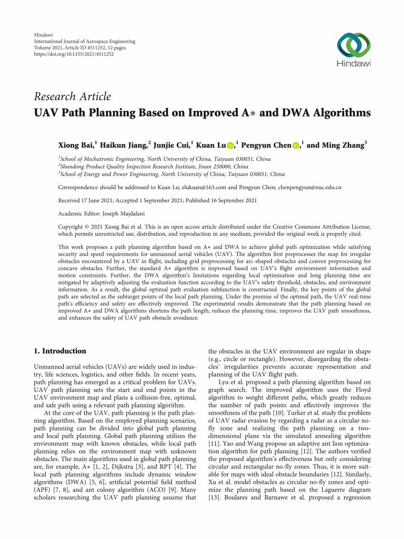
2.2. Gridding Treatment of Arc Obstacles. This paper utilizesthe idea of a rough set to obtain a polygon approximatingthe arc-shaped obstacles [21]. The main method first deter-mines a grid of the arc obstacle’s outer edge line, along withits positioning grid. Then, the polygon processing is per-formed, and each arc grid’s positioning points are con-nected, as shown in Figure 1(b). The specific steps are asfollows:

(Step 1) Determine the outer edge line (L) of the arcobstacle (B). Further, determine the grid posi-tion of each arc line Li, and denote the markedgrid elements as Mi. Regard the centers of themarked grid elements as the locating points,and denote them as Pi, i = 1, 2,⋯, n, where nis the number of segments of the outer edge line

(Step 2) Connect the locating points P1, P2,⋯, Pn, P1,obtaining the polygon P1P2 ⋯ PnP1 by regard-ing each M1,M2,⋯,Mn,M1 clockwise fromthe starting marked grid element. Conse-quently, obtain the result of obstacle B polygonprocessing, B ≈ P1, P2 ⋯ PnP1

2.3. Convex Filling of Concave Polygon Obstacles. The convexfilling process commences by determining the coordinates ofeach polygon vertex in the grid graph. Starting from the first

2 International Journal of Aerospace Engineering

grid element, the polygon vertices are denoted S1, S2,⋯, Sm,where m is the number of vertices of the polygon. If theinner angle formed by the two adjacent edges is greater than180 degrees, the corresponding vertex Si is a concave point.Otherwise, the vertex is a convex point. In the path-searching algorithm, if the path point falls into the concavearea, the next path point must be placed outside the concavearea to complete the flight mission. Concave areas affect theUAV path quality and increase the number of invalid pathpoints, affecting the solution speed.

Figure 2 shows an example of the convex filling process.The steps are as follows.

(Step 1) Determine the concave polygon’s vertices S1,S2,⋯, S7, and judge the concavity and convex-ity of each vertex according to the concavityand convexity rules (Figure 2(a))

(Step 2) Based on Step 1, start from the starting convexpoint S1, and connect other convex pointsclockwise, yielding the polygon S1S3S4S5S6S1as the convex result (i.e., F ≈ S1S3S4S5S6S1).Then, the obstacles are gridded according tothe arc obstacles, as shown in Figure 2(b)

3. Improved A∗ Algorithm

There are many turning points and large angles in the pathplanned via the standard A∗, which is not conducive to aUAV flight. Thus, this work improves the standard A∗according to the motion characteristics and environmentalinformation of UAVs in flight.

3.1. Improvement of the Heuristic Function. The evaluationfunction of A∗ is composed of a cost function gðnÞ and aheuristic function hðnÞ, and the algorithm’s optimal search-

ing performance depends on the selection of the heuristicfunction. The improved A∗ algorithm introduces the obsta-cle weight coefficient into the heuristic function, as shown inEquation (2). The obstacle weight coefficient expresses thegrid map complexity, and the environmental informationis analyzed.

The obstacle weight coefficient is defined as the propor-tion of the number of obstacles in the current map and thenumber of grid cells in the whole grid map. Let N standfor the number of obstacle grid cells and denote UAV start-ing and ending coordinates as ðxs, ysÞ and ðxg, ygÞ, respec-tively. The obstacle weight coefficient is defined as

K = N

xs − xg�� ��� �

× ys − yg��� ���� �  K ∈ 0, 1ð Þð Þ, ð1Þ

f nð Þ = a ∗ g nð Þ + π

2 − arctan K� �

∗ h nð Þ, ð2Þ

where gðnÞ is the cost from the starting node to the currentnode, hðnÞ is the heuristic function value from the currentnode to the target node, ðxn, ynÞ are the current node’s coor-dinates, and a is the weight of the cost function gðnÞ. Thecoefficient a is calculated as the ratio of the distance fromthe current node to the target point and the distance fromthe starting node to the target point.

According to equation (2), the improved algorithm setsthe weight of the adaptive heuristic function. When theobstacle weight coefficient K is small, the weight of the heu-ristic function is increased. The A∗ algorithm reduces thesearch space, improves the speed of path planning, andeffectively reduces the inflection points and turning pointsof the path. When the obstacle weight coefficient is large,reduce the weight of the heuristic function and increase the

(a)

MiPi

B

L

(b)

Figure 1: Comparison of the gridding treatment for arc-shaped obstacles. (a) Before treatment. (b) After treatment.

3International Journal of Aerospace Engineering

search space to avoid the algorithm falling into localoptimization.

3.2. Determining the UAV Safety Distance. The improved A∗sets the safety distance between the path node and the obsta-cle to prevent the UAV from colliding with the obstacle. Asshown in Figure 3, the vertical distance OE (the vertical dis-tance from point O to line KG) from the obstacle to the pathis compared with the preset safety distance to judge whetherthe planned path is safe and feasible.

Suppose the coordinates of node K are ðx1, y1Þ, and thecoordinates of target node G are ðx2, y2Þ. Denote the coordi-nates of obstacle node O as ðx3, y3Þ and the coordinates ofnode F as ðx4, y4Þ. The length of line segment OF, denotedas l, is the distance between the obstacle and line segmentKG along the longitudinal axis. The angle between line KGand the x-axis is α, whereas d denotes the distance fromthe obstacle to the path. The specific principle is as follows:

l = y3 − y4j j, ð3Þ

y4 =y2 − y1x2 − x1

x3 − x1ð Þ + y1

� �, ð4Þ

α = arctan y1 − y2x1 − x2

��������, ð5Þ

d = l cos α: ð6ÞThe distance d from the obstacle to the path is calculated

following equation (6). Let D denote the safety threshold.Then, distance d is compared with the safety distance D todetermine whether the path can be used as an alternativepath. If d ≤D, the path is abandoned. Then, according tothe improved A∗ algorithm, continue to search for newnodes until the optimal path is found. Otherwise (i.e., whend >D), the path is selected.

3.3. Path Smoothing Optimization. As emphasized previ-ously, because the algorithm search principle and subnodesearch direction of standard A∗ algorithm are 8-node

S1

S2

S4

S3

S5

S6

S7

(a)

S1

S2

S4

S3

S5

S6

S7

(b)

Figure 2: The convex filling of a concave polygon. (a) Before treatment. (b) After treatment.

y

C x

K d

E

F

l

O

S

G

Figure 3: Safety distance design.

y

O x

G

S7

S8

S6

S5S

4

S3S

2

S1

S

Figure 4: Floyd algorithm smoothing path comparison.

4 International Journal of Aerospace Engineering

expansion direction, the path planned by the algorithm isnot conducive to UAV flight. Further, path planning takesa long time, and the search route is close to the obstacle’sedge. The improved A∗ algorithm combines the Floyd algo-rithm with the A∗ algorithm, effectively reducing the num-ber of turning points in the UAV path [22], improving theUAV movement efficiency, and meeting the UAV applica-tion requirements. Considering the kinematic model tojudge whether the derived path is more suitable than theoriginal regarding distance, time, and angle, the algorithmoptimization path comparison is shown in Figure 4.

As shown in Figure 4, the standard A∗ algorithm yieldsthe path (S, S1, S2, S3, S4, S5, S6, S7, S8,G). This path has manyinflection points, resulting in poor smoothness.

The Floyd smoothing algorithm can be used to eliminateredundant path nodes, effectively reducing the number ofturns and optimizing the path length. The Floyd algorithmcombines the UAV motion characteristics to improve thepath smoothness. By judging whether there is an obstaclebetween the two nodes, as well as considering the securitythreshold D and the distance d between the two nodes con-nected to the obstacle, one can determine whether the pathis feasible. Finally, the path (S, S1, S7,G) is obtained.

Building on the described principles, the standard A∗algorithm and the improved A∗ algorithm are simulatedand verified, and the obtained paths are shown in Figure 5.

The path planned by the standard A∗ algorithm(Figure 5(a)) has many redundant nodes and road sections,and its turning angles are large. As a result, the path lengthis 75.1543 km, which is suboptimal (i.e., not the shortest)and does not conform to the UAV operation rules. In con-trast, the path planned by the improved A∗ algorithm(Figure 5(b)) is relatively smooth, and its length equals72.0735 km. Thus, the improved algorithm achieves a4.1% improvement in the path length. Moreover, a certainsafety distance can be observed between the global pathand the obstacles, which is more conducive to the UAVmovement.

4. Improved DWA

In the local path planning, the standard DWA algorithmonly specifies the position of the target point, failing to con-sider unknown obstacles. Moreover, when there are manyobstacles, the path planning algorithm easily falls into thelocal optimum, resulting in an increase in the global pathlength. The improved A∗ algorithm regards the global path’skey nodes as subtarget points of the local path. Then, theenvironmental information is used to adjust the weight coef-ficient in the speed evaluation subfunction. Consequently,UAVs can successfully avoid unknown obstacles and reachthe target point safely and efficiently.

4.1. Motion Model. The basic idea of DWA [6, 23, 24] is topredict the UAV’s velocity vector space and state vectorspace at a particular time, simulate the UAV’s trajectory atthe predicted time, and finally select the optimal trajectorybased on the evaluation function. Assuming that the UAVis moving in a uniform manner at every time interval Δt,the UAV kinematics model is as follows:

x tnð Þ = x t0ð Þ +ðtnt0

Vr tð Þ cos θ tð Þ½ �dt,

y tnð Þ = y t0ð Þ +ðtnt0

Vr tð Þ sin θ tð Þ½ �dt,

θ tnð Þ = θ t0ð Þ + ω tð ÞΔt,

8>>>>>>><>>>>>>>:

ð7Þ

where xðtnÞ, yðtnÞ, and θðtnÞ are the position coordinatesand attitude angle coordinates of UAV in world coordinatesat time t and VrðtÞ is the dynamic window (further intro-duced in the next section).

4.2. UAV Speed Sampling. DWA models the UAV’s obstacleavoidance problem as an optimization problem with velocityconstraints, including nonholonomic constraints, environ-mental obstacle constraints, and UAV dynamic constraints.

50

40

30

20

10

00 10 20 30 40 50

(a)

50

40

30

20

10

00 10 20 30 40 50

(b)

Figure 5: Comparison of the standard A∗ and the improved A∗ path planning results. (a) Standard A∗ algorithm. (b) Improved A∗algorithm.

5International Journal of Aerospace Engineering

The DWA’s velocity vector space diagram is shown inFigure 6. The abscissa and ordinate represent the UAVangular velocity (w) and the UAV linear velocity (v). Inaccordance, vmax and vmin denote the maximum and mini-mum linear velocity, whereas wmax and wmin are the maxi-mum and minimum angular velocities. The whole area isVs, the white area (Va) represents the safe area, and Vd isthe UAV speed range considering motor torque limitationin the control cycle. Finally, Vr is the UAV dynamic windowdetermined by the intersection of the listed three sets.

According to the UAV speed limit, Vs is the set of theUAV’s linear velocity and angular velocity fitting withinthe maximum dynamic window range:

Vs = v,wð Þ vmin≤v≤vmax,wmin≤w≤wmax

�� : ð8Þ

The UAV’s motion trajectory can be subdivided intoseveral linear or circular motions. In order to ensure thesafety of UAV, under the condition of maximum decelera-tion, the current speed of UAV shall be able to hover in acertain accuracy range in the air before encountering obsta-cles, and the speed shall approach 0. The linear velocity andangular velocity set Va near obstacles is defined as

Va = v,wð Þ v≤ffiffiffiffiffiffiffiffiffiffiffiffiffiffiffiffiffi2dist v,wð Þ _vb

p,w≤

ffiffiffiffiffiffiffiffiffiffiffiffiffiffiffiffiffiffi2dist v,wð Þ _wb

p���n o, ð9Þ

where _vb is the UAV’s maximum linear deceleration, _wb isthe UAV’s maximum angular deceleration, and distðv,wÞis the shortest distance between the path and the obstacle.

The UAV motor torque’s limitations influence the max-imum and minimum attainable velocities v and w in a cer-tain time t. Thus, the dynamic window needs to be furtherreduced. Given the current linear velocity vc and angularvelocity wc, the dynamic window Vd at the next periodmeets the following requirements:

Vd = v,wð Þ vc− _vbΔt≤v≤vc+ _vaΔt,wc− _wbΔt≤w≤ _waΔt

�� , ð10Þ

where _va is the UAV’s maximum linear acceleration and _wais the UAV’s maximum angular acceleration.

The final speed range is the set at the intersection of thethree discussed sets, and the dynamic window Vr is definedas follows:

Vr = Vs ∩Va ∩Vd: ð11Þ

The continuous velocity vector space (Vr) is discretizedbased on the number of linear velocity and angular velocitysamples to obtain the discrete sampling points (v,w). Foreach sampling point, the UAV motion trajectory at the nextmoment is predicted using the UAV kinematics model (seeFigure 7).

4.3. Adaptive DWA Algorithm. DWA controls the speedusing the weight coefficient (β) in the speed evaluation sub-function. If β is too large, the UAV is very fast, but the safetyis reduced. In contrast, if β is too small, the UAV’s speed isinsufficient, but the safety is very high. Considering the rela-

tionship between UAV safety and speed, the improvedDWA algorithm adaptively calculates the speed evaluationfunction’s weight coefficient while relying on environmentalinformation. The UAV’s sensors are utilized to collectenvironmental information. The obstacle density and thedistance between the UAV and the obstacles in the environ-ment are used to calculate the speed evaluation function’sweight coefficient. The weight coefficient is adjusted toachieve higher speed in safe areas, whereas the speed isreduced in dangerous areas to enhance UAV flight safety.

4.3.1. Safety Threshold for Obstacle Detection. The distance Lbetween different obstacles is calculated using the distanceand angle between obstacles and the UAV. The specific cal-culation formula is as follows:4

L =ffiffiffiffiffiffiffiffiffiffiffiffiffiffiffiffiffiffiffiffiffiffiffiffiffiffiffiffiffiffiffiffiffiffiffiffiffiffiffiffiffiffiffiffiffiffiD2i +D2

j − 2DiDj cos θð Þq

, Di ≤Dj, ð12Þ

where Di and Dj are the distances between i-th and j-thobstacles and the UAV and θ is the angle between theUAV and the obstacles.

The distance between different obstacles serves to judgewhether the UAV can pass through the obstacles. When Lequals more than twice the two obstacles’ expansion dis-tance, the UAV can pass between the obstacles.

4.3.2. Adaptive Function Calculation. The UAV safetydepends on the shortest distance between the UAV andthe obstacle (denoted Dmin), which serves as the input for

Va

Vs

v

Vd

wmin

Vr

wmax w

Figure 6: Schematic diagram of the velocity vector space.

Y (m)

X (m)

(vc – v

bΔt, w

c + w

aΔt)

(vc + v

bΔt, w

c + w

aΔt)

(vc + v

aΔt, w

c – w

bΔt)

(vc – v

bΔt, w

c – w

bΔt)

(vc, w

c)

Figure 7: UAV trajectory prediction.

6 International Journal of Aerospace Engineering

the adaptive dynamic function. The threshold Dl is definedas

Dl = n ⋅vmax_v

� �, ð13Þ

where vmax is the UAV’s highest speed, _v is the UAV’s linearacceleration, and n is the parameter. Dl is directly propor-tional to the maximum speed vmax and inversely propor-tional to the linear acceleration _v. Thus, the stronger theUAV’s braking force, the smaller the threshold. The fasterthe speed, the larger the threshold, ensuring the UAV’ssafety.

The relationship between the speed evaluation function’sweight coefficient βr and input Dmin is as follows:

βr = β0‐ηeDmin/Ds , Dmin ≤Ds, β0,Dmin >Ds

: ð14Þ

If the UAV flight is within the safety threshold (i.e. theshortest distance Dmin between the UAV and the obstacleis less than the UAV safety threshold, the UAV flight speedwas reduced (according to the nature of exponential func-tion). If the UAV flies outside the safety threshold (i.e., theshortest distance Dmin between the UAV and obstacles isgreater than the UAV safety threshold), the UAV flightspeed is set according to the maximum speed weight, asshown in equation (14).

β0 is the maximum speed weight, Ds is the safety thresh-old, and η is the adjustment parameter. When Ds is greaterthan Dmin, the speed weight increases monotonically withthe input Dmin, i.e., βr = β0. When Ds is less than Dmin, thespeed weight is an exponential function of Ds and Dmin. Asthe ratio of Dmin and Ds decreases, βr increases. Otherwise,if Dmin/Ds increases, βr decreases.

4.3.3. Improved Evaluation Function. The standard DWAalgorithm does not refer to the UAV’s global path but onlyplans the target points. Moreover, in the case of numerousobstacles, the process easily falls into a local optimum, yield-ing a larger path distance. The distðv,wÞ weight in theevaluation function moves the UAV trajectory away fromobstacles, resulting in a locally optimal trajectory andincreasing the global moving distance. If the correspondingweighting coefficient (γ) is directly reduced, the UAV facedwith the unknown obstacles cannot avoid them in time,leading to the collision.

To solve the described problems, the azimuth evaluationfunction headingðv,wÞ is designed, which integrates theglobal path’s nodes. Let velðv,wÞ denote the evaluation func-tion of the current simulation speed. Two different obstacleevaluation functions, dist sðv,wÞ and dist dðv,wÞ, aredesigned. dist sðv,wÞ is defined as the evaluation functionfor predicting the shortest distance between the end pointof the trajectory and the globally known obstacle. Similarly,dist dðv,wÞ is the evaluation function for predicting theshortest distance between the end point of the trajectoryand the unknown obstacle. The trajectory evaluation func-tion is as follows:

G v,wð Þ = α ⋅ heading v,wð Þ + βr ⋅ vel v,wð Þ + γ ⋅ dist s vwð Þ+ λ ⋅ dist d v,wð Þ,

ð15Þ

where α, βr, γ, and λ are the coefficients of the four evaluations.

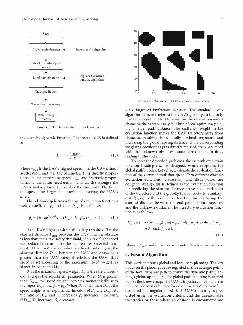
5. Fusion Algorithm

This work combines global and local path planning. The keynodes on the global path are regarded as the subtarget pointsof the local dynamic path to ensure the dynamic path plan-ning’s global optimality. The global path planning is carriedout on the known map. The UAV’s trajectory information inthe next period is calculated based on the UAV’s current lin-ear speed and angular speed. Each UAV trajectory is pre-dicted using the evaluation criteria, and the unreasonabletrajectories or those where an obstacle is encountered are

Start

Global path planning

Extract the critical pathnodes

Local path planning

Improved A⁎ algorithm

Track prediction

The optimal trajectory

Improved dynamicwindow algorithm

Path findingsuccess

Figure 8: The fusion algorithm’s flowchart.

50

40

30

20

10

00 10 20 30 40 50

Figure 9: The initial UAV airspace environment.

7International Journal of Aerospace Engineering

discarded. The path evaluation subfunction evaluates a cer-tain path, and the evaluation values are accumulated. Thetrajectory with the lowest cost is deemed as the optimal tra-jectory. If the current optimal trajectory is passable, theUAV moves with the speed corresponding to the optimaltrajectory. The UAV avoids the encountered obstacles basedon the obstacle avoidance rules. The flowchart of theimproved algorithm is shown in Figure 8.

6. Simulation Experiment and Analysis

6.1. Experiment Environment. The main simulation environ-ment consisted of an Intel (R) Core I i5-8265U CPU@1.60GHz, Windows10, and the simulations were con-ducted in MATLAB. A 50 km × 50 km path planning areaand the corresponding grid map were established to verifythe algorithm’s effectiveness. The UAV’s maximum turning

Table 1: Path planning results when the obstacles are known.

Algorithm Path length (km) Time (s) Speed increase rate

Improved A∗ algorithm 73.9423 0.2405

Standard DWA algorithm 77.8257 3427.26731.6%

Fusion of the improved A∗ and DWA algorithms 75.6582 2531.638

Table 2: Path planning results when the obstacles are unknown.

Algorithm Path length (km) Time (s) Speed increase rate

Improved A∗ algorithm 73.9423 0.2405

Standard DWA algorithm 78.5025 3023.20634.2%

Fusion of the improved A∗ and DWA algorithms 76.5843 1942.824

50

40

30

20

10

00 10 20 30 40 50

(a)

50

40

30

20

10

00 10 20 30 40 50

(b)

50

40

30

20

10

00 10 20 30 40 50

(c)

Figure 10: Comparison of the path planning algorithms on known maps. (a) Improved A∗ algorithm. (b) Standard DWA algorithm. (c)Fusion of improved A∗ and DWA algorithms.

8 International Journal of Aerospace Engineering

angle was assumed to equal π/4. In the simulation, the gridgranularity was set so that N = 1 km, the safety thresholdequaled 0.8 km, and the UAV’s starting and ending coordi-nates were (0.5, 0.5) and (49.5, 49.5). The UAV’s flight envi-ronment is obtained by grid processing of arc obstacles andconvex processing of concave obstacles. The UAV’s initialairspace is shown in Figure 9.

6.2. Simulation Studies on Path Planning with Known andUnknown Obstacles

6.2.1. Path Planning in the Initial Airspace Environment. Thesimulation experiment compared the improved A∗ algo-rithm, the standard DWA algorithm, and the fusion of A∗and DWA algorithms to obtain the planning time and theresulting path’s length. The results are shown in Table 1.

The simulation results (Table 2 and Figure 10) demon-strate that the improved A∗ algorithm plans a globally opti-mal path. Compared with the improved A∗ algorithm, thepath planned using the standard DWA algorithm issmoother but not globally optimal. Further, the plannedpath is not based on the planned global path, meaning thereare several redundant paths. In Figure 10(c), the DWA algo-

rithm combines the global path planning and considers theenvironmental information during the UAV’s flight. Conse-quently, the weight coefficient of the speed evaluationsubfunction is adaptively adjusted, effectively reducing theUAV path planning time. Simultaneously, the obstacles aredistinguished to reduce the impact of the known obstacleson the evaluation function, and the planned path is shortand close to the global planning path.

According to Table 1, the length of the path plannedusing the fusion of improved A∗ and DWA algorithm isreduced by 2.8% compared to that obtained via the standardDWA algorithm. Further, the planning time is reduced by26.3%, and the average UAV’s flight speed is increased by31.6%.

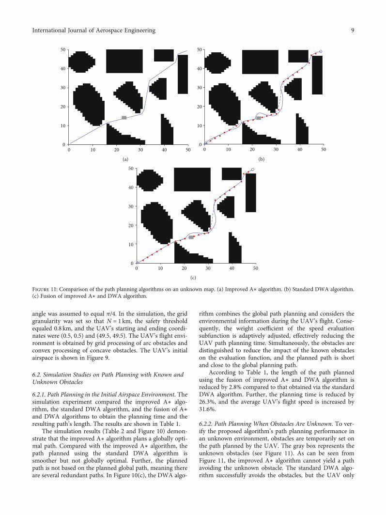
6.2.2. Path Planning When Obstacles Are Unknown. To ver-ify the proposed algorithm’s path planning performance inan unknown environment, obstacles are temporarily set onthe path planned by the UAV. The gray box represents theunknown obstacles (see Figure 11). As can be seen fromFigure 11, the improved A∗ algorithm cannot yield a pathavoiding the unknown obstacle. The standard DWA algo-rithm successfully avoids the obstacles, but the UAV only

50

40

30

20

10

00 10 20 30 40 50

(a)

50

40

30

20

10

00 10 20 30 40 50

(b)

50

40

30

20

10

00 10 20 30 40 50

(c)

Figure 11: Comparison of the path planning algorithms on an unknown map. (a) Improved A∗ algorithm. (b) Standard DWA algorithm.(c) Fusion of improved A∗ and DWA algorithm.

9International Journal of Aerospace Engineering

starts to bypass the obstacles when near them, enhancing theprobability of a collision. In the case depicted inFigure 11(b), the UAV cannot fly along the initially plannedglobal path, and there are many redundant paths, increasingthe UAV’s flight distance. By combining the improved A∗algorithm and DWA algorithm, the local path planningcan be realized, and the unknown obstacles can be avoidedeffectively. The local path is similar to the global path, prov-ing that a smooth and safe path can be obtained.

Similar to the experiment reported in Section 6.2.1, thesimulation experiment compared the improved A∗ algo-

rithm, the standard DWA algorithm, and the fusion of A∗and DWA algorithms. The obtained path planning timeand the path length are shown in Table 2.

As seen in Table 2, the improved A∗ and DWA algo-rithm reduces the planned path’s length by 2.4% comparedwith the standard DWA algorithm. Further, the planningtime decreases by 35.7%, whereas the average UAV’s flightspeed increases by 34.2%.

Next, environmental maps of different sizes were createdto obtain environments of different complexity. The mapranges were set to 10 ∗ 10, 20 ∗ 20, 30 ∗ 30, 40 ∗ 40, and

80

70

60

Fusion of improved A⁎ and DWA algorithm

Standard DWA algorithm

50

40

Dist

ance

(km

)30

20

10

010⁎10 20⁎20

Number30⁎30 40⁎40 50⁎50

Figure 12: The relationship between the map size and the length of the paths yielded by the two algorithms.

Fusion of improved A⁎ and DWA algorithm

Standard DWA algorithm

10⁎10 20⁎20Number

30⁎30 40⁎40 50⁎50

3500

3000

2500

2000

Tim

e (s)

1500

1000

500

0

Figure 13: The relationship between the map size and the planning time planning of the two algorithms.

10 International Journal of Aerospace Engineering

50 ∗ 50. The shortest path length and path planning timeunder different environmental maps were extracted(Figures 12 and 13).

As shown in Figure 12, the increase in map size results inan increase in the UAV’s flight path. Compared with thestandard DWA algorithm, the average path planned by thefusion of the improved A∗ and DWA algorithms is reducedby 4.22%. The advantages of the improved A∗ and DWAalgorithm become more pronounced with the increase inmap size. Figure 13 shows that the path planning time ofthe fused improved A∗ and DWA algorithms is significantlyshorter than that of the standard DWA. In addition, theincrease in map size highlights the advantages of the pro-posed improved A∗ and DWA algorithm, signaling thatthe algorithm is more conducive to the UAV’s path planningin a wide range.

7. Conclusion

This work alleviates the shortcomings in terms of smooth-ness and security of the path planned using the standardA∗ algorithm and tackles the problem of the standardDWA algorithm regarding its proneness to falling into alocal optimum. The paper proposes a path planning algo-rithm that combines the improved A∗ algorithm and theDWA algorithm, leveraging the two algorithms’ advantagesand reducing their limitations. The main conclusions areas follows:

(1) Through grid modeling of an irregular map, thiswork establishes grid processing of arc obstaclesand convex processing of concave obstacles

(2) Environment information and motion constraintsare utilized to improve the A∗ algorithm. Whencompared to the standard A∗ algorithm, the pathplanned by the improved A∗ algorithm is smoother,and the UAV’s motion safety is guaranteed

(3) An adaptive DWA is designed to dynamically adjustthe path evaluation function using the safety thresh-old, UAV information, and environmental informa-tion regarding the obstacles

(4) The key nodes in the global path planned by theimproved A∗ algorithm serve as the subtargets forthe local path planning. Such a design ensures theoptimal global path and improves the UAV’s real-time path planning efficiency and safety

(5) The experimental results show that the pathplanning based on the fusion of improved A∗ andDWA algorithms effectively reduces the path length,shortens the UAV’s path planning time, andimproves both the path smoothness and the safetyof the local obstacle avoidance

Data Availability

The data used to support the findings of this study areavailable from the corresponding author upon request.

Conflicts of Interest

The authors declare that there is no conflict of interestregarding the publication of this paper.

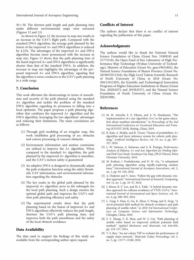
Acknowledgments

The authors would like to thank the National NaturalScience Foundation of China (Grant Nos. 51909245 and51775518), the Open Fund of Key Laboratory of High Per-formance Ship Technology (Wuhan University of Technol-ogy), Ministry of Education (Grant No. gxnc19051802), theNatural Science Foundation of Shanxi Province (Grant No.201901D211244), the High-Level Talents Scientific Researchof North University of China in 2018 (Grant No.304/11012305), the Scientific and Technological InnovationPrograms of Higher Education Institutions in Shanxi (GrantNos. 2020L0272 and 2019L0537), and the Natural ScienceFoundation of North University of China (Grant No.XJJ201908).

References

[1] M. M. Attoyibi, F. E. Fikrisa, and A. N. Handayani, “Theimplementation of a star algorithm (A∗) in the game educa-tion about numbers introduction,” in Proceedings of the 2ndInternational Conference on Vocational Education and Train-ing (ICOVET 2018), Beijing, China, 2019.

[2] R. Kala, A. Shukla, and R. Tiwari, “Fusion of probabilistic A∗algorithm and fuzzy inference system for robotic path plan-ning,” Artificial Intelligence Review, vol. 33, no. 4, pp. 307–327, 2010.

[3] L. W. Santoso, A. Setiawan, and A. K. Prajogo, PerformanceAnalysis of Dijkstra, A∗ and Ant Algorithm for Finding Opti-mal Path Case Study: Surabaya City Map, [Ph.D.Tthesis], PetraChristian University, 2010.

[4] M. Kothari, I. Postlethwaite, and D. W. Gu, “A suboptimalpath planning algorithm using rapidly-exploring randomtrees,” International Journal of Aerospace Innovations, vol. 2,no. 1, pp. 93–104, 2010.

[5] A. Özdemir and V. Sezer, “Follow the gap with dynamic win-dow approach,” International Journal of Semantic Computing,vol. 12, no. 1, pp. 43–57, 2018.

[6] J. Moon, B.-Y. Lee, and M.-J. Tahk, “A hybrid dynamic win-dow approach for collision avoidance of VTOL UAVs,” Inter-national Journal of Aeronautical and Space Sciences, vol. 19,no. 4, pp. 889–903, 2018.

[7] L. Tang, S. Dian, G. Gu, K. Zhou, S. Wang, and X. Feng, “Anovel potential field method for obstacle avoidance and pathplanning of mobile robot,” in 2010 3rd International Confer-ence on Computer Science and Information Technology,Chengdu, China, 2010.

[8] S. Y. Zhang, Y. K. Shen, and W. S. Cui, “Path planning ofmobile robot based on improved artificial potential fieldmethod,” Applied Mechanics and Materials, vol. 644-650,pp. 154–157, 2014.

[9] T. S. Rao, “An ant colony TSP to evaluate the performance ofsupply chain network,” Materials Today: Proceedings, vol. 5,no. 5, pp. 13177–13180, 2018.

11International Journal of Aerospace Engineering

[10] D. Lyu, Z. Chen, Z. Cai, and S. Piao, “Robot path planning byleveraging the graph-encoded Floyd algorithm,” Future Gener-ation Computer Systems, vol. 122, pp. 204–208, 2021.

[11] T. Turker, O. K. Sahingoz, and G. Yilmaz, “2D path planningfor UAVs in radar threatening environment using simulatedannealing algorithm,” in 2015 International Conference onUnmanned Aircraft Systems (ICUAS), Denver, CO, USA, 2015.

[12] P. Yao and H. Wang, “Dynamic adaptive ant lion optimizerapplied to route planning for unmanned aerial vehicle,” SoftComputing, vol. 21, no. 18, pp. 5475–5488, 2017.

[13] Z. Xu, R. Wei, K. Zhou, Q. Zhang, and R. He, “Laguerre graphself-optimize path planning algorithm for UAVs in irregularobstacle environment,” in 2016 IEEE Chinese Guidance, Navi-gation and Control Conference (CGNCC), Nanjing, China,2016.

[14] M. Boulares and A. Barnawi, “A novel UAV path planningalgorithm to search for floating objects on the ocean surfacebased on object's trajectory prediction by regression,” Roboticsand Autonomous Systems, vol. 135, article 103673, 2021.

[15] A. Belkadi, H. Abaunza, L. Ciarletta, P. Castillo, andD. Theilliol, “Distributed path planning for controlling a fleetof UAVs : application to a team of quadrotors ∗∗research sup-ported by the Conseil Regional de Lorraine, the Ministére deL’Education Nationale, de l’Enseignement Supérieur et de LaRecherche, and the National Network of Robotics Platforms(ROBOTEX), from France,” IFAC-PapersOnLine, vol. 50,no. 1, pp. 15983–15989, 2017.

[16] L. Huang, H. Qu, P. Ji, X. Liu, and Z. Fan, “A novel coordi-nated path planning method using k -degree smoothing formulti-UAVs,” Applied Soft Computing, vol. 48, pp. 182–192,2016.

[17] D. Yulong, X. Bin, C. Jie et al., “Path planning of messengerUAV in air-ground coordination,” IFAC-PapersOnLine,vol. 50, no. 1, pp. 8045–8051, 2017.

[18] L. Huo, J. Zhu, Z. Li, and M. Ma, “A hybrid differential symbi-otic organisms search algorithm for UAV path planning,” Sen-sors, vol. 21, no. 9, 2021.

[19] M. D. Phung and Q. P. Ha, “Safety-enhanced UAV path plan-ning with spherical vector-based particle swarm optimiza-tion,” Applied Soft Computing, vol. 107, article 107376, 2021.

[20] V. Jeauneau, L. Jouanneau, and A. Kotenkoff, “Path plannermethods for UAVs in real environment,” IFAC-PapersOnLine,vol. 51, no. 22, pp. 292–297, 2018.

[21] Z. Yuan, H. Chen, T. Li, Z. Yu, B. Sang, and C. Luo, “Unsuper-vised attribute reduction for mixed data based on fuzzy roughsets,” Information Sciences, vol. 572, pp. 67–87, 2021.

[22] J. Wang, Y. Sun, Z. Liu, P. Yang, and T. Lin, “Route planningbased on Floyd algorithm for intelligence transportation sys-tem,” in 2007 IEEE International Conference on IntegrationTechnology, Shenzhen, China, 2007.

[23] X. Ji, S. Feng, Q. Han, H. Yin, and S. Yu, “Improvement andfusion of A∗ algorithm and dynamic window approach con-sidering complex environmental information,” Arabian Jour-nal for Science and Engineering, vol. 46, no. 8, pp. 7445–7459, 2021.

[24] D. Feng, L. Deng, T. Sun, H. Liu, H. Zhang, and Y. Zhao, LocalPath Planning Based on an Improved Dynamic WindowApproach in ROS, Springer, 2021.

12 International Journal of Aerospace Engineering