An Evaluation of UAV Path Following Algorithms

P.B. Sujit, Srikanth Saripalli, J.B. Sousa

Abstract— Path following is the simplest desired autonomousnavigation capability for UAVs. Several approaches have beendeveloped in the literature for path following. However, thereis no adequate information on the comparison analysis ofthese algorithms. In this paper, we compare five path followingalgorithms that are easy to implement, take less implementationtime and are robust to disturbances. The comparison of theseguidance laws is carried out through simulations using the totalcross-track error and control effort performance metrics.

I. INTRODUCTION

With low cost sensors, electronics and airframes, there is agreat interest in using unmanned aerial vehicles (UAVs) forseveral non-military applications like habitat mapping, aerialphotogrammetry, agriculture, marine sciences, etc. Most ofthese missions require the UAV to autonomously followpredefined paths at constant height. The common paths beingstraight line paths and circular orbits (called as loiter). Thepath following algorithms must be accurate in following thepath and robust to wind disturbances.

In the literature, several path following algorithms havebeen well developed for unmanned aerial vehicles, underwa-ter vehicles, surface vehicles and ground vehicles. The basicfunctionality of path following for any type of unmannedvehicle is the same as the guidance laws developed for pathfollowing use kinematic constraints with constant velocity.Although, several types of path following algorithms areavailable in the literature, there is no adequate informationon the comparison between different algorithms in terms ofperformance or the implementation time.

In this paper, we provide an overview of path followingproblem, describe different path following algorithms fromthe literature and characterize their performance based onaccuracy, robustness and control effort. The selected pathfollowing algorithms are carrot following algorithm, non-linear guidance law (NLGL) [1], vector field based pathfollowing (VF) [2], linear quadratic regulator based pathfollowing (LQR) [3], and pure pursuit and line-of-sight basedpath following (PLOS) [4]. These algorithms were mainlyselected due to their simplicity and ease of implementation.

There are several other types of path following algorithmsusing guidance approaches [5], [6], and advanced controlconcepts [7], [8], [9], [10], [11], [12]. The PLOS and

P.B. Sujit is a Research Scientist in the Department of Electrical andComputer Engineering, University of Porto, Portugal - 4200-165. Email- sujit@fe.up.pt

Srikanth Saripalli is Asst. Professor in the School of Earth andSpace Exploration, University of Arizona, Tempe, AZ 85287. Email -srikanth.saripalli@asu.edu

J.B. Sousa is Asst. Professor in the Department of Electrical andComputer Engineering, University of Porto, Portugal - 4200-165. Email- jtasso@fe.up.pt

LQR based path following algorithms consider some ofguidance concepts similar to [5], [6]. The NLGL and VF pathfollowing algorithms have been proven theoretically usingLyapunov based stability conditions in [1], [2] similar to[7], [8], [9], [10], [11]. Silva and Sousa [12] use dynamicprogramming approach which is difficult to implement.Since the selected path following algorithms [1], [2], [3],[4] address some principles used in other path followingalgorithms, we do not consider them for analysis. In thispaper, by using a kinematic model and simulating variouspath following strategies we are able to demonstrate theadvantages and disadvantages of each one of them and studythe effect of change in parameters.

A. Path following problemGiven a path, initial location p = (x, y) of the aerial

vehicle along with its heading angle (ψ), the path followingproblem is to determine the commanded heading angle (ψd)for the vehicle such that by following (ψd), the UAV accu-rately tracks the path as the mission progresses. Typically,for most of the missions either straight line paths or circularorbit paths are used. The straight line paths can be defined asa set of waypoints (as shown in Fig 1(a)). The angle formedby waypoints Wi and Wi+1 is called the line-of-sight (LOS)angle. Figure 1(b) shows the initial geometry for a circularorbit also called loiter following. Assume that the UAV is ata distance d from the path. This distance d is called as cross-track error. Apart from minimizing the cross-track error, theUAV must ensure that ψ is same as the LOS angle θ. Theobjective of the path following algorithms is to minimized → 0 and |ψ − θ| → 0, where |.| represents the absolutevalue as the mission time t→∞.

B. OrganizationThe rest of the paper is organized as follows. In Section II,

we describe different path following algorithms for straightline and loiter paths, and analyze their behavior for differentparameter variations. In Section III, we compare the per-formance of path following algorithms and we conclude inSection IV.

II. PATH FOLLOWING ALGORITHMS

The two most commonly used paths for UAVs are straightlines and loiter paths. Both the type of paths are usuallydefined on a xy plane with constant altitude and speed. Underthis assumption, we can model the UAV kinematics as

x = va cosψ + vw cos(ψw) = vg cosχ,

y = va sinψ + vw sin(ψw) = vg sinχ,

ψ = χ = u, (1)

2013 European Control Conference (ECC)July 17-19, 2013, Zürich, Switzerland.

978-3-952-41734-8/©2013 EUCA 3332

(a) (b)

x

y

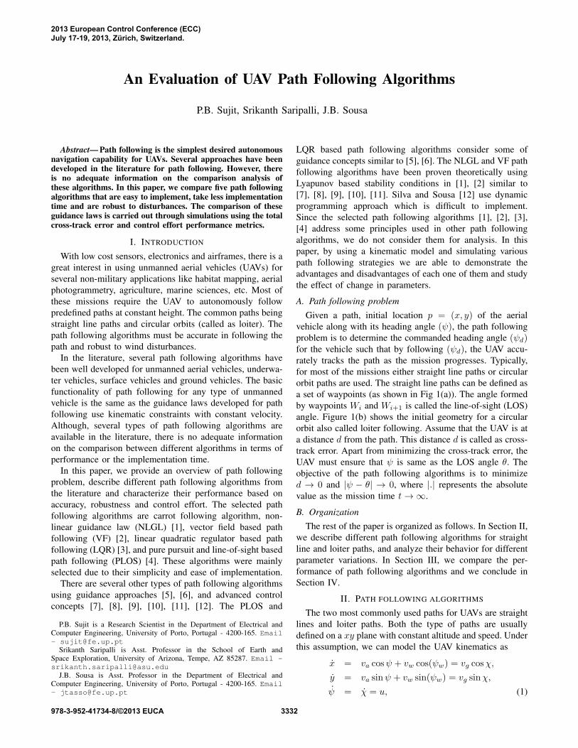
Fig. 1. (a) The UAV has to follow a straight line path (b) The UAV hasto follow a loiter or orbit of radius r

where va m/s is the UAV airspeed, ψ is the UAV headingheading angle, ψ is the heading angle rate which is con-strained by −ωmax < ψ < ωmax, vw m/s is the wind speedin the ψw rad direction and u is the control. When the windcomponent is not considered then va and ψ are used, whileunder the influence of wind, the equations with ground speedvg =

√(va cosψ + vw cosψw)2 + (va sinψ + vw sinψw)2

and course angle χ = atan2(y, x) are considered. Thekinematic model of the UAV represents a Dubins car model[18]. For all the simulations in this paper, we considerva = 15m/s with minimum turning radius of 45m. Theconsidered loiter circle is of radius r = 100m.

In order to analyze the working principle of the algorithmsand performance under different parameter conditions, weconsidered the kinematic model without wind for simplicity.However, in Section III, we will consider the presence ofwind for performance comparison.

A. Carrot chasing algorithm

A simplest approach to follow a desired path is to intro-duce a virtual target point (VTP) on the path and direct theUAV to chase VTP. As the engagement progresses, the UAVapproaches towards the path and eventually follow the path.In this approach, the VTP is called the Carrot and the UAVchases the carrot, hence the name Carrot chasing algorithm.

1) Straight line following: Consider a straight line asshown in Figure 1(a). Following a straight line path involvestwo steps: (i) determining the cross-track error (d) and (ii)updating the location of the virtual target. Let the cross-trackerror of the path be d. The VTP (s) is located at a distanceδ from q as shown in Figure 1(a). The UAV desired heading(ψd) is updated based on the location of s. The process offinding new ψd continues until the UAV reaches Wi+1. Theprocedure to update the location of VTP and ψd is given inAlgorithm 1.

The control input u in Algorithm 1 uses a proportionalcontroller with gain κ > 0. The path parameter δ can modifythe performance of the carrot chasing algorithm as shown inFigure 2(a). For low δ = 0− 10, the UAV is forced to movetowards the LOS and it takes longer time to settle on thepath resulting in higher cross-track error. With increase in δthe UAV is able to settle on the path quickly, thus reducingthe cross-track error. However, with large δ, the cross-track

Algorithm 1 Algorithms for carrot chasing algorithmStraight Line following

1: Initialize: Wi = (xi, yi),Wi+1 = (xi+1, yi+1), p =(x, y), ψ

2: Ru = ||Wi − p||, θ = atan2(yi+1 − yi, xi+1 − xi)3: θu = atan2(y − yi, x− xi), β = θ − θu4: R =

√R2

u − (Ru sin(β))2

5: (x′t, y′t)← ((R+ δ) cos θ, (R+ δ) sin θ) % s = (x′t, y

′t)

6: ψd = atan2(y′t − y, x′t − x)7: u = κ(ψd − ψ)

Loiter following1: Initialize: O = (xl, yl), r, p, ψ2: d = ||O − p|| − r3: θ = atan2(y − yl, x− xl)4: (x′t, y

′t)← (r cos(θ + λ), r sin(θ + λ)) % s = (x′t, y

′t)

5: ψd = atan2(y′t − y, x′t − x)6: u = κ(ψd − ψ)

0 50 100 150 200 250 300 350 400

0

50

100

150

200

250

300

350

400

X in meters

Y i

n m

eter

s

path

δ=0

δ=10

δ=30

δ=50

(a)

−150 −100 −50 0 50 100 150 200−150

−100

−50

0

50

100

150

X in meters

Y in m

ete

rs

λ=0.2

loiter path

λ=0.4λ=0.1

λ=0

λ=1

(b)

Fig. 2. Performance of the carrot chasing algorithm with variation in δand λ (a) UAV trajectories for different δ (b) The vehicle trajectories whenλ is varied.

again increases but the time taken to reach W1 decreases asthe UAV moves ahead towards W1.

2) Loiter: In loiter maneuver, the UAV is tasked to circlearound a point (O) with a standoff distance of r meters asshown in Figure 1(b). To loiter, the UAV must be locatedon the circle and its heading direction must be orthogonalto the line Oq. Assume the UAV is located at p and thecross-track error is d = ||O − p|| − r. Using the cross-trackerror information and the direction of loiter, we can generatea VTP (s in the Figure 1(b)). The procedure to update theUAV and the VTP is given in Algorithm 1.

The path parameter λ needs to be selected properly toensure quicker path convergence. When λ = 0, the UAVis unable to track the path as the desired VTP alwayspoints orthogonal to the UAV position causing it to performsinusoidal path along the loiter as shown in Figure 2(b).When λ is increased to λ = 0.1, 0.2, 0.4 radians, the UAVtracks the loiter circle quickly. However, with further increasein λ = 1 radian, the UAV is unable to track the path as theVTP is always further away.

B. Non-linear guidance law

The non-linear guidance law (NLGL) was developed byPark et al. [1], which uses the VTP concept, but the mecha-

3333

(a)

x

y

(b)

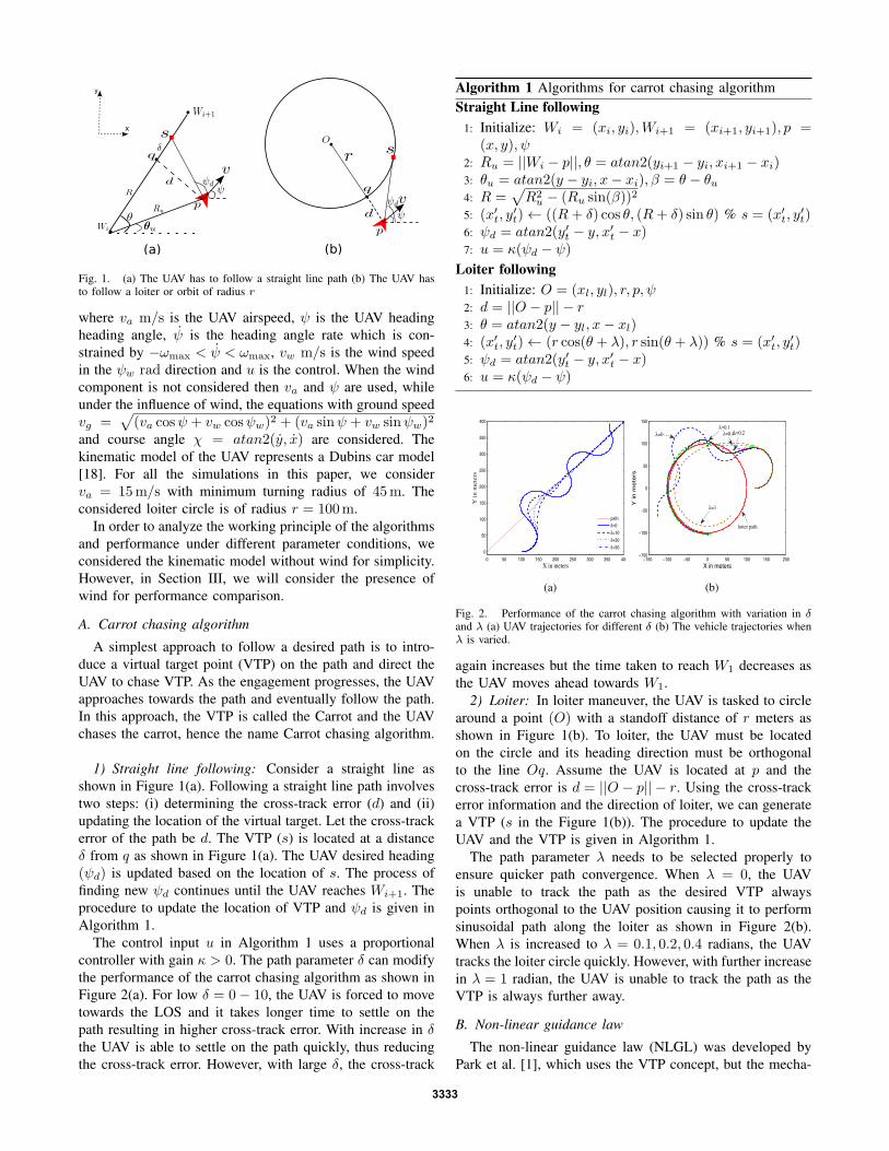
Fig. 3. (a) Determining the intersection point for VTP q and q′ (b)Geometry for pure pursuit and LOS based path following algorithm

0 50 100 150 200 250 300 350 4000

50

100

150

200

250

300

350

400

X in meters

YX

in m

ete

rs

L =30

L =50

L =80

L =120

L =100

UAVPath

(a)

−150 −100 −50 0 50 100 150 200−150

−100

−50

0

50

100

150

X in meters

Y in

me

ters

L =30L =50

L=80 L =100

Loiter pathUAV position

(b)

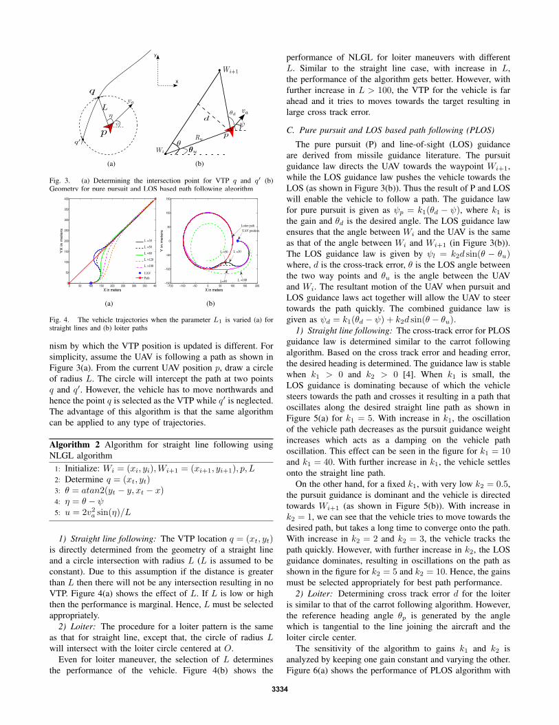
Fig. 4. The vehicle trajectories when the parameter L1 is varied (a) forstraight lines and (b) loiter paths

nism by which the VTP position is updated is different. Forsimplicity, assume the UAV is following a path as shown inFigure 3(a). From the current UAV position p, draw a circleof radius L. The circle will intercept the path at two pointsq and q′. However, the vehicle has to move northwards andhence the point q is selected as the VTP while q′ is neglected.The advantage of this algorithm is that the same algorithmcan be applied to any type of trajectories.

Algorithm 2 Algorithm for straight line following usingNLGL algorithm

1: Initialize: Wi = (xi, yi),Wi+1 = (xi+1, yi+1), p, L2: Determine q = (xt, yt)3: θ = atan2(yt − y, xt − x)4: η = θ − ψ5: u = 2v2a sin(η)/L

1) Straight line following: The VTP location q = (xt, yt)is directly determined from the geometry of a straight lineand a circle intersection with radius L (L is assumed to beconstant). Due to this assumption if the distance is greaterthan L then there will not be any intersection resulting in noVTP. Figure 4(a) shows the effect of L. If L is low or highthen the performance is marginal. Hence, L must be selectedappropriately.

2) Loiter: The procedure for a loiter pattern is the sameas that for straight line, except that, the circle of radius Lwill intersect with the loiter circle centered at O.

Even for loiter maneuver, the selection of L determinesthe performance of the vehicle. Figure 4(b) shows the

performance of NLGL for loiter maneuvers with differentL. Similar to the straight line case, with increase in L,the performance of the algorithm gets better. However, withfurther increase in L > 100, the VTP for the vehicle is farahead and it tries to moves towards the target resulting inlarge cross track error.

C. Pure pursuit and LOS based path following (PLOS)

The pure pursuit (P) and line-of-sight (LOS) guidanceare derived from missile guidance literature. The pursuitguidance law directs the UAV towards the waypoint Wi+1,while the LOS guidance law pushes the vehicle towards theLOS (as shown in Figure 3(b)). Thus the result of P and LOSwill enable the vehicle to follow a path. The guidance lawfor pure pursuit is given as ψp = k1(θd − ψ), where k1 isthe gain and θd is the desired angle. The LOS guidance lawensures that the angle between Wi and the UAV is the sameas that of the angle between Wi and Wi+1 (in Figure 3(b)).The LOS guidance law is given by ψl = k2d sin(θ − θu)where, d is the cross-track error, θ is the LOS angle betweenthe two way points and θu is the angle between the UAVand Wi. The resultant motion of the UAV when pursuit andLOS guidance laws act together will allow the UAV to steertowards the path quickly. The combined guidance law isgiven as ψd = k1(θd − ψ) + k2d sin(θ − θu).

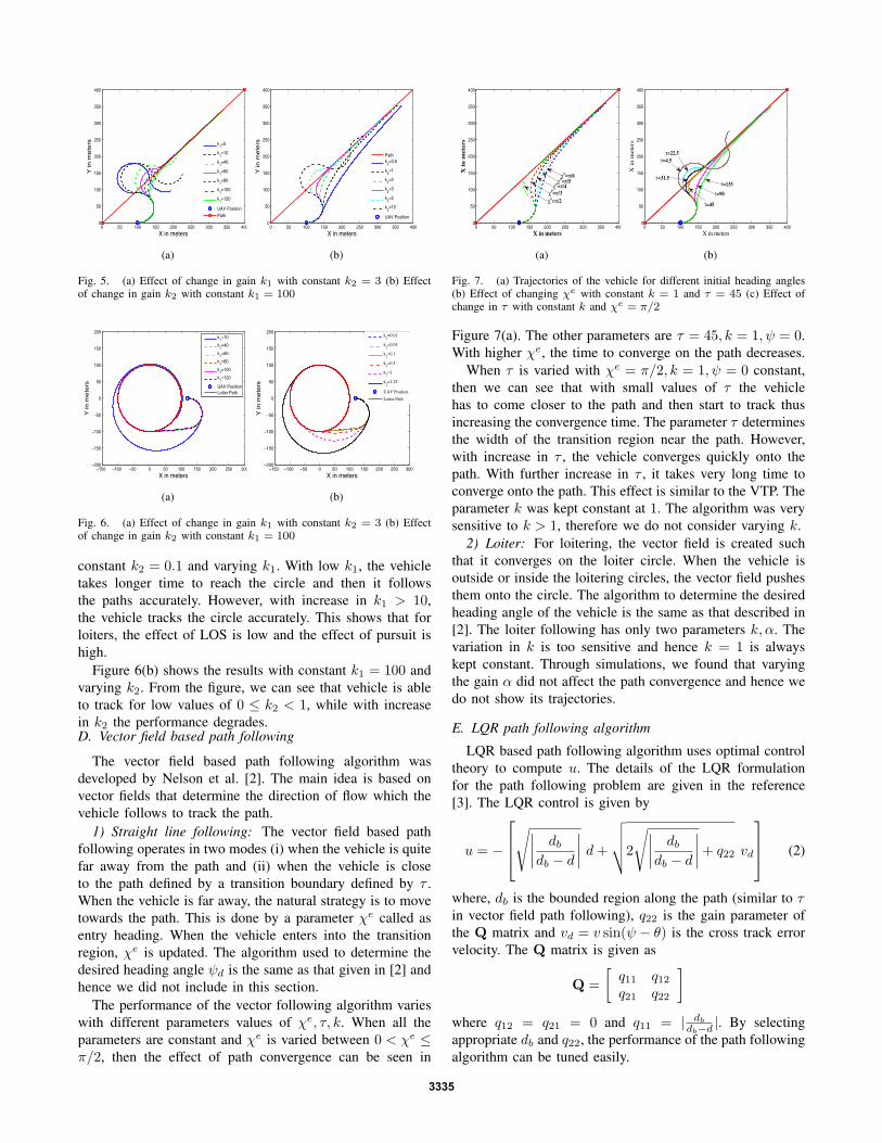
1) Straight line following: The cross-track error for PLOSguidance law is determined similar to the carrot followingalgorithm. Based on the cross track error and heading error,the desired heading is determined. The guidance law is stablewhen k1 > 0 and k2 > 0 [4]. When k1 is small, theLOS guidance is dominating because of which the vehiclesteers towards the path and crosses it resulting in a path thatoscillates along the desired straight line path as shown inFigure 5(a) for k1 = 5. With increase in k1, the oscillationof the vehicle path decreases as the pursuit guidance weightincreases which acts as a damping on the vehicle pathoscillation. This effect can be seen in the figure for k1 = 10and k1 = 40. With further increase in k1, the vehicle settlesonto the straight line path.

On the other hand, for a fixed k1, with very low k2 = 0.5,the pursuit guidance is dominant and the vehicle is directedtowards Wi+1 (as shown in Figure 5(b)). With increase ink2 = 1, we can see that the vehicle tries to move towards thedesired path, but takes a long time to converge onto the path.With increase in k2 = 2 and k2 = 3, the vehicle tracks thepath quickly. However, with further increase in k2, the LOSguidance dominates, resulting in oscillations on the path asshown in the figure for k2 = 5 and k2 = 10. Hence, the gainsmust be selected appropriately for best path performance.

2) Loiter: Determining cross track error d for the loiteris similar to that of the carrot following algorithm. However,the reference heading angle θp is generated by the anglewhich is tangential to the line joining the aircraft and theloiter circle center.

The sensitivity of the algorithm to gains k1 and k2 isanalyzed by keeping one gain constant and varying the other.Figure 6(a) shows the performance of PLOS algorithm with

3334

0 50 100 150 200 250 300 350 4000

50

100

150

200

250

300

350

400

X in meters

Y in m

ete

rs

k1=5

k1=10

k1=40

k1=60

k1=80

k1=100

k1=120

UAV PositionPath

(a)

0 50 100 150 200 250 300 350 4000

50

100

150

200

250

300

350

400

X in meters

Y in m

ete

rs

Pathk

2=0.5

k2=1

k2=2

k2=3

k2=5

k2=10

UAV Position

(b)

Fig. 5. (a) Effect of change in gain k1 with constant k2 = 3 (b) Effectof change in gain k2 with constant k1 = 100

−150 −100 −50 0 50 100 150 200 250 300−200

−150

−100

−50

0

50

100

150

200

X in meters

Y in m

ete

rs

k

1=10

k1=40

k1=60

k1=80

k1=100

k1=120

UAV PositionLoiter Path

(a)

−150 −100 −50 0 50 100 150 200 250 300−200

−150

−100

−50

0

50

100

150

200

X in meters

Y in

mete

rs

k

2=0.01

k2=0.05

k2=0.1

k2=0.5

k2=1

k2=1.25

UAV Position

Loiter Path

(b)

Fig. 6. (a) Effect of change in gain k1 with constant k2 = 3 (b) Effectof change in gain k2 with constant k1 = 100

constant k2 = 0.1 and varying k1. With low k1, the vehicletakes longer time to reach the circle and then it followsthe paths accurately. However, with increase in k1 > 10,the vehicle tracks the circle accurately. This shows that forloiters, the effect of LOS is low and the effect of pursuit ishigh.

Figure 6(b) shows the results with constant k1 = 100 andvarying k2. From the figure, we can see that vehicle is ableto track for low values of 0 ≤ k2 < 1, while with increasein k2 the performance degrades.D. Vector field based path following

The vector field based path following algorithm wasdeveloped by Nelson et al. [2]. The main idea is based onvector fields that determine the direction of flow which thevehicle follows to track the path.

1) Straight line following: The vector field based pathfollowing operates in two modes (i) when the vehicle is quitefar away from the path and (ii) when the vehicle is closeto the path defined by a transition boundary defined by τ .When the vehicle is far away, the natural strategy is to movetowards the path. This is done by a parameter χe called asentry heading. When the vehicle enters into the transitionregion, χe is updated. The algorithm used to determine thedesired heading angle ψd is the same as that given in [2] andhence we did not include in this section.

The performance of the vector following algorithm varieswith different parameters values of χe, τ, k. When all theparameters are constant and χe is varied between 0 < χe ≤π/2, then the effect of path convergence can be seen in

0 50 100 150 200 250 300 350 4000

50

100

150

200

250

300

350

400

X i

n m

eter

s

X in meters

χe=π/2χe=π/3

χe=π/4χe=π/5

χe=π/6

(a)

0 50 100 150 200 250 300 350 4000

50

100

150

200

250

300

350

400

X i

n m

eter

s

X in meters

τ=4.5τ=22.5

τ=31.5

τ=45

τ=90

τ=135

(b)

Fig. 7. (a) Trajectories of the vehicle for different initial heading angles(b) Effect of changing χe with constant k = 1 and τ = 45 (c) Effect ofchange in τ with constant k and χe = π/2

Figure 7(a). The other parameters are τ = 45, k = 1, ψ = 0.With higher χe, the time to converge on the path decreases.

When τ is varied with χe = π/2, k = 1, ψ = 0 constant,then we can see that with small values of τ the vehiclehas to come closer to the path and then start to track thusincreasing the convergence time. The parameter τ determinesthe width of the transition region near the path. However,with increase in τ , the vehicle converges quickly onto thepath. With further increase in τ , it takes very long time toconverge onto the path. This effect is similar to the VTP. Theparameter k was kept constant at 1. The algorithm was verysensitive to k > 1, therefore we do not consider varying k.

2) Loiter: For loitering, the vector field is created suchthat it converges on the loiter circle. When the vehicle isoutside or inside the loitering circles, the vector field pushesthem onto the circle. The algorithm to determine the desiredheading angle of the vehicle is the same as that described in[2]. The loiter following has only two parameters k, α. Thevariation in k is too sensitive and hence k = 1 is alwayskept constant. Through simulations, we found that varyingthe gain α did not affect the path convergence and hence wedo not show its trajectories.

E. LQR path following algorithm

LQR based path following algorithm uses optimal controltheory to compute u. The details of the LQR formulationfor the path following problem are given in the reference[3]. The LQR control is given by

u = −

√∣∣∣∣ db

db − d

∣∣∣∣ d+√√√√2

√∣∣∣∣ dbdb − d

∣∣∣∣+ q22 vd

(2)

where, db is the bounded region along the path (similar to τin vector field path following), q22 is the gain parameter ofthe Q matrix and vd = v sin(ψ − θ) is the cross track errorvelocity. The Q matrix is given as

Q =

[q11 q12q21 q22

]where q12 = q21 = 0 and q11 = | db

db−d |. By selectingappropriate db and q22, the performance of the path followingalgorithm can be tuned easily.

3335

−150 −100 −50 0 50 100 150 200 250 300−200

−150

−100

−50

0

50

100

150

200

X in meters

Y in m

ete

rs

Pathq

22=0.1

q22

=0.5

q22

=1

q22

=5

q22

=10

q22

=20

UAV Position

(a)

0 50 100 150 200 250 300 350 4000

50

100

150

200

250

300

350

400

X in meters

Y in m

ete

rs

Pathq

22=0.1

q22

=0.5

q22

=1

q22

=2

q22

=5

q22

=10

UAV Position

(b)

Fig. 8. Performance of the adaptive LQR path following algorithm for (a)loiter path with different q22 values and (b) with different q22 values for astraight line path

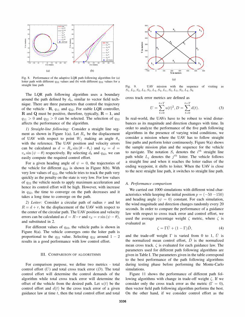
The LQR path following algorithm uses a boundaryaround the path defined by db, similar to vector field tech-nique. There are three parameters that control the trajectoryof the vehicle - R, q11 and q22. For stable LQR controller,R and Q must be positive, therefore, typically, R = 1, andq11 > 0 and q22 > 0 can be selected. The selection of q22affects the performance of the algorithm.

1) Straight-line following: Consider a straight line seg-ment as shown in Figure 1(a). Let Ru be the displacementof UAV with respect to point W1 making an angle θuwith the reference. The UAV position and velocity errorscan be calculated as d = Ru sin (θ − θv) and vd = d =va sin (ψ − θ) respectively. By selecting db and q22, we caneasily compute the required control effort.

For a given heading angle of ψ = 0, the trajectories ofthe vehicle for different q22 is shown in Figure 8(b). Withvery low values of q22, the vehicle tries to track the path veryquickly as the penalty on the state is very low. For low valuesof q22 the vehicle needs to apply maximum acceleration andhence its control effort will be high. However, with increasein q22, the time to converge on the path decreases and ittakes a long time to converge on the path.

2) Loiter: Consider a circular path of radius r and letR = d+ r, be the displacement of the UAV with respect tothe center of the circular path. The UAV position and velocityerrors can be calculated as d = R−r and vd = v sin (ψ − θ),and substituted in 2.

For different values of q22, the vehicle paths is shown inFigure 8(a). The vehicle converges onto the loiter path isproportional to the q22 value. Selecting q22 around 1 − 2results in a good performance with low control effort.

III. COMPARISON OF ALGORITHMS

For comparison purpose, we define two metrics - totalcontrol effort (U ) and total cross track error (D). The totalcontrol effort will determine the control demands of thealgorithm while total cross track error will determine theoffset of the vehicle from the desired path. Let u(t) be thecontrol effort and d(t) be the cross track error of a givenguidance law at time t, then the total control effort and total

−100 0 100 200 300 400 500 600−100

0

100

200

300

400

500

600

X in meters

Y in

met

ers

S1

S2

S3

S4

S5

L1

L2

L3L

4

S6

(a)

Fig. 9. UAV mission with the sequence of visiting asS1, L2, S2, L3, S3, L4, S4, L1, S5, L3, S3, L4, S6

cross track error metrics are defined as

U =t=T∑t=0

u(t)2, D =t=T∑t=0

d(t). (3)

In real-world, the UAVs have to be robust to wind distur-bances as its magnitude and direction changes with time. Inorder to analyze the performance of the five path followingalgorithms in the presence of varying wind conditions, weconsider a mission where the UAV has to follow straightline paths and perform loiter continuously. Figure 9(a) showsthe sample mission plan and the sequence for the vehicleto navigate. The notation Si denotes the ith straight linepath while Lj denotes the jth loiter. The vehicle followsa straight line and when it reaches the loiter radius of theending waypoint, it shifts to loiter. When the UAV is closeto the next straight line path, it switches to straight line path.

A. Performance comparison

We carried out 1000 simulations with different wind char-acteristics while keeping the initial position p = (−50 −150)and heading angle (ψ = 0) constant. For each simulation,the wind magnitude and direction changes randomly every 20seconds. In order to compare the performance of a guidancelaw with respect to cross track error and control effort, weused the average percentage weight ζ metric, where ζ isevaluated as

ζ = ΓU + (1− Γ)D, (4)

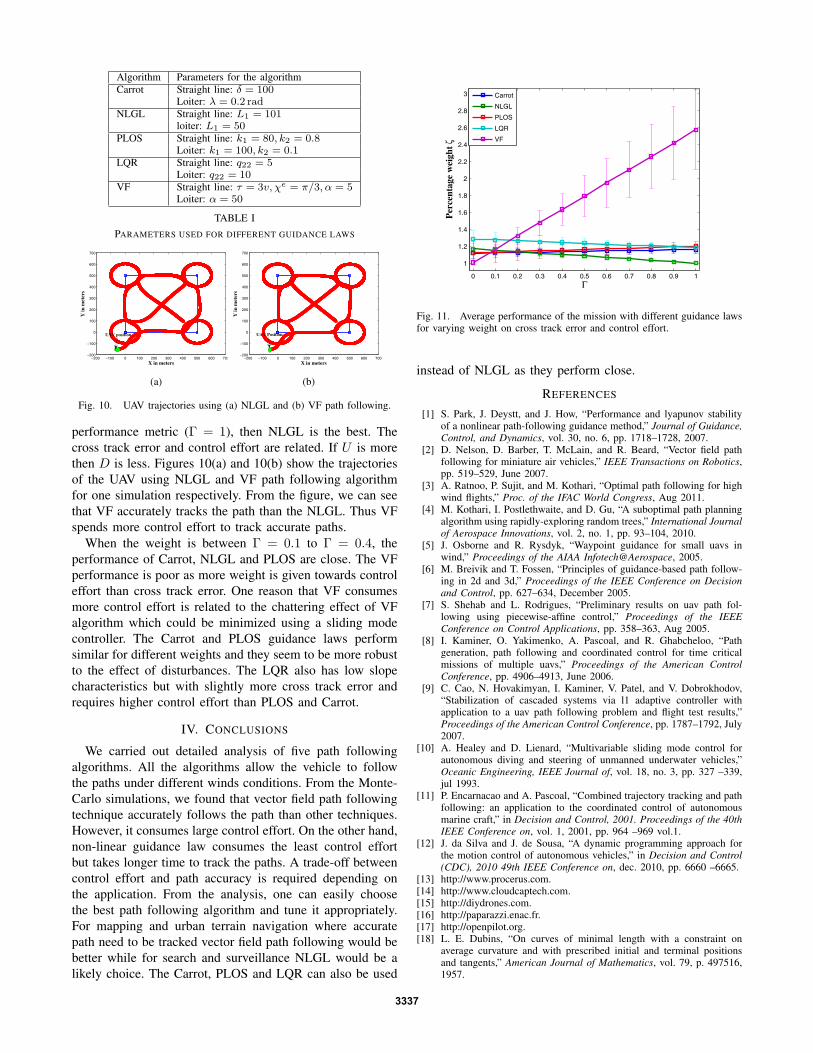
and the trade-off weight Γ is varied from 0 to 1, U isthe normalized mean control effort, D is the normalizedmean cross track. ζ is evaluated for each guidance law. Theparameters used for different path following algorithms aregiven in Table I. The parameters given in the table correspondto the best performance of the path following algorithmsduring testing phase before performing the Monte-Carlosimulations.

Figure 11 shows the performance of different path fol-lowing algorithms with change in trade-off weight ζ. If weconsider only the cross track error as the metric (Γ = 0),then vector field path following algorithm performs the best.On the other hand, if we consider control effort as the

3336

Algorithm Parameters for the algorithmCarrot Straight line: δ = 100

Loiter: λ = 0.2 radNLGL Straight line: L1 = 101

loiter: L1 = 50PLOS Straight line: k1 = 80, k2 = 0.8

Loiter: k1 = 100, k2 = 0.1LQR Straight line: q22 = 5

Loiter: q22 = 10VF Straight line: τ = 3v, χe = π/3, α = 5

Loiter: α = 50

TABLE IPARAMETERS USED FOR DIFFERENT GUIDANCE LAWS

−200 −100 0 100 200 300 400 500 600 700−200

−100

0

100

200

300

400

500

600

700

X in meters

Y in

met

ers

UAV position

(a)

−200 −100 0 100 200 300 400 500 600 700−200

−100

0

100

200

300

400

500

600

700

X in meters

Y in

met

ers

UAV Position

(b)

Fig. 10. UAV trajectories using (a) NLGL and (b) VF path following.

performance metric (Γ = 1), then NLGL is the best. Thecross track error and control effort are related. If U is morethen D is less. Figures 10(a) and 10(b) show the trajectoriesof the UAV using NLGL and VF path following algorithmfor one simulation respectively. From the figure, we can seethat VF accurately tracks the path than the NLGL. Thus VFspends more control effort to track accurate paths.

When the weight is between Γ = 0.1 to Γ = 0.4, theperformance of Carrot, NLGL and PLOS are close. The VFperformance is poor as more weight is given towards controleffort than cross track error. One reason that VF consumesmore control effort is related to the chattering effect of VFalgorithm which could be minimized using a sliding modecontroller. The Carrot and PLOS guidance laws performsimilar for different weights and they seem to be more robustto the effect of disturbances. The LQR also has low slopecharacteristics but with slightly more cross track error andrequires higher control effort than PLOS and Carrot.

IV. CONCLUSIONS

We carried out detailed analysis of five path followingalgorithms. All the algorithms allow the vehicle to followthe paths under different winds conditions. From the Monte-Carlo simulations, we found that vector field path followingtechnique accurately follows the path than other techniques.However, it consumes large control effort. On the other hand,non-linear guidance law consumes the least control effortbut takes longer time to track the paths. A trade-off betweencontrol effort and path accuracy is required depending onthe application. From the analysis, one can easily choosethe best path following algorithm and tune it appropriately.For mapping and urban terrain navigation where accuratepath need to be tracked vector field path following would bebetter while for search and surveillance NLGL would be alikely choice. The Carrot, PLOS and LQR can also be used

0 0.1 0.2 0.3 0.4 0.5 0.6 0.7 0.8 0.9 1

1

1.2

1.4

1.6

1.8

2

2.2

2.4

2.6

2.8

3

Γ

Per

cent

age

wei

ght ζ

Carrot

NLGL

PLOS

LQR

VF

Fig. 11. Average performance of the mission with different guidance lawsfor varying weight on cross track error and control effort.

instead of NLGL as they perform close.

REFERENCES

[1] S. Park, J. Deystt, and J. How, “Performance and lyapunov stabilityof a nonlinear path-following guidance method,” Journal of Guidance,Control, and Dynamics, vol. 30, no. 6, pp. 1718–1728, 2007.

[2] D. Nelson, D. Barber, T. McLain, and R. Beard, “Vector field pathfollowing for miniature air vehicles,” IEEE Transactions on Robotics,pp. 519–529, June 2007.

[3] A. Ratnoo, P. Sujit, and M. Kothari, “Optimal path following for highwind flights,” Proc. of the IFAC World Congress, Aug 2011.

[4] M. Kothari, I. Postlethwaite, and D. Gu, “A suboptimal path planningalgorithm using rapidly-exploring random trees,” International Journalof Aerospace Innovations, vol. 2, no. 1, pp. 93–104, 2010.

[5] J. Osborne and R. Rysdyk, “Waypoint guidance for small uavs inwind,” Proceedings of the AIAA Infotech@Aerospace, 2005.

[6] M. Breivik and T. Fossen, “Principles of guidance-based path follow-ing in 2d and 3d,” Proceedings of the IEEE Conference on Decisionand Control, pp. 627–634, December 2005.

[7] S. Shehab and L. Rodrigues, “Preliminary results on uav path fol-lowing using piecewise-affine control,” Proceedings of the IEEEConference on Control Applications, pp. 358–363, Aug 2005.

[8] I. Kaminer, O. Yakimenko, A. Pascoal, and R. Ghabcheloo, “Pathgeneration, path following and coordinated control for time criticalmissions of multiple uavs,” Proceedings of the American ControlConference, pp. 4906–4913, June 2006.

[9] C. Cao, N. Hovakimyan, I. Kaminer, V. Patel, and V. Dobrokhodov,“Stabilization of cascaded systems via l1 adaptive controller withapplication to a uav path following problem and flight test results,”Proceedings of the American Control Conference, pp. 1787–1792, July2007.

[10] A. Healey and D. Lienard, “Multivariable sliding mode control forautonomous diving and steering of unmanned underwater vehicles,”Oceanic Engineering, IEEE Journal of, vol. 18, no. 3, pp. 327 –339,jul 1993.

[11] P. Encarnacao and A. Pascoal, “Combined trajectory tracking and pathfollowing: an application to the coordinated control of autonomousmarine craft,” in Decision and Control, 2001. Proceedings of the 40thIEEE Conference on, vol. 1, 2001, pp. 964 –969 vol.1.

[12] J. da Silva and J. de Sousa, “A dynamic programming approach forthe motion control of autonomous vehicles,” in Decision and Control(CDC), 2010 49th IEEE Conference on, dec. 2010, pp. 6660 –6665.

[13] http://www.procerus.com.[14] http://www.cloudcaptech.com.[15] http://diydrones.com.[16] http://paparazzi.enac.fr.[17] http://openpilot.org.[18] L. E. Dubins, “On curves of minimal length with a constraint on

average curvature and with prescribed initial and terminal positionsand tangents,” American Journal of Mathematics, vol. 79, p. 497516,1957.

3337