Trends, RB-k Assign 8,9
14
Trends –assignment 8 & Randomized Block Design – assignment 9 For discussion during our first Easter class day… Have a restful, blessed, reflective week…
description
Trends, RB-k Assign 8,9
Transcript of Trends, RB-k Assign 8,9

Trends –assignment 8&
Randomized Block Design – assignment 9For discussion during our first Easter class day…
Have a restful, blessed, reflective week…

AS
failure
failure
trendAfailuretrendAfailure
AS
trendtrend
trend
trendtrendjtrendtrend
MS
MSF
dfdfdfSSSSSS
MS
MSF
c
nSSYc
j
/
/
2
2
;
;
Trends Analysis - Formulas
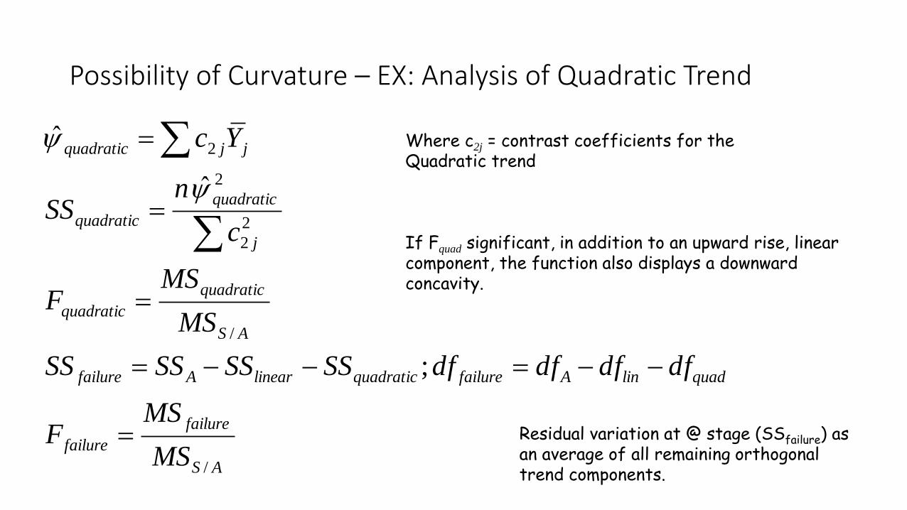
Possibility of Curvature – EX: Analysis of Quadratic Trend
AS
failure
failure
quadlinAfailurequadraticlinearAfailure
AS
quadratic
quadratic
j
quadratic
quadratic
jjquadratic
MS
MSF
dfdfdfdfSSSSSSSS
MS
MSF
c
nSS
Yc
/
/
2
2
2
2
;
ˆ
ˆ
Where c2j = contrast coefficients for the Quadratic trend
If Fquad significant, in addition to an upward rise, linear component, the function also displays a downward concavity.
Residual variation at @ stage (SSfailure) as an average of all remaining orthogonal trend components.

Higher order trends…
...3
3
2
210
'
2
210
'
jjjj
jjj
XbXbXbbY
XbXbbY
Single concavity or bend – quadratic concave up or concave down (inverted U)
Residual variation evaluated by Ffailure = average of all remaining orthogonal trend components (additional trends could be masked)
Finding the simplest function that describes the data
Capturing tendency for function to rise or fall over range of X and tendency for function to be curved
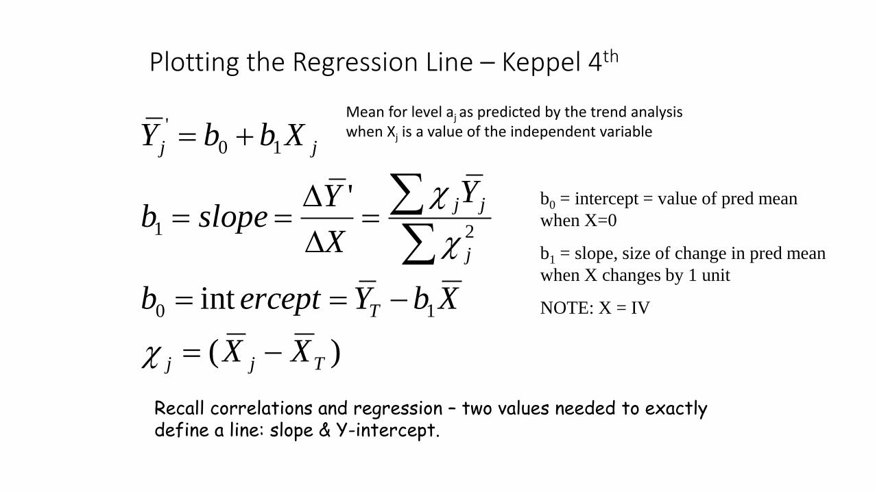
Plotting the Regression Line – Keppel 4th
)(
int
'
10
21
10
'
Tjj
T
j
jj
jj
XX
XbYerceptb
Y
X
Yslopeb
XbbY
Recall correlations and regression – two values needed to exactly define a line: slope & Y-intercept.
Mean for level aj as predicted by the trend analysis when Xj is a value of the independent variable
b0 = intercept = value of pred mean
when X=0
b1 = slope, size of change in pred mean
when X changes by 1 unit
NOTE: X = IV

...'
...
)(
int
'
3
3
2
210
3
3
2
210
10
21
10
'
jjjj
Tjj
T
j
jj
jj
XbXbXbbY
XbXbXbbY
XX
XbYerceptb
Y
X
Yslopeb
XbbY
To get values for b2 regress Y mean for group j onto Xj and Xj
2
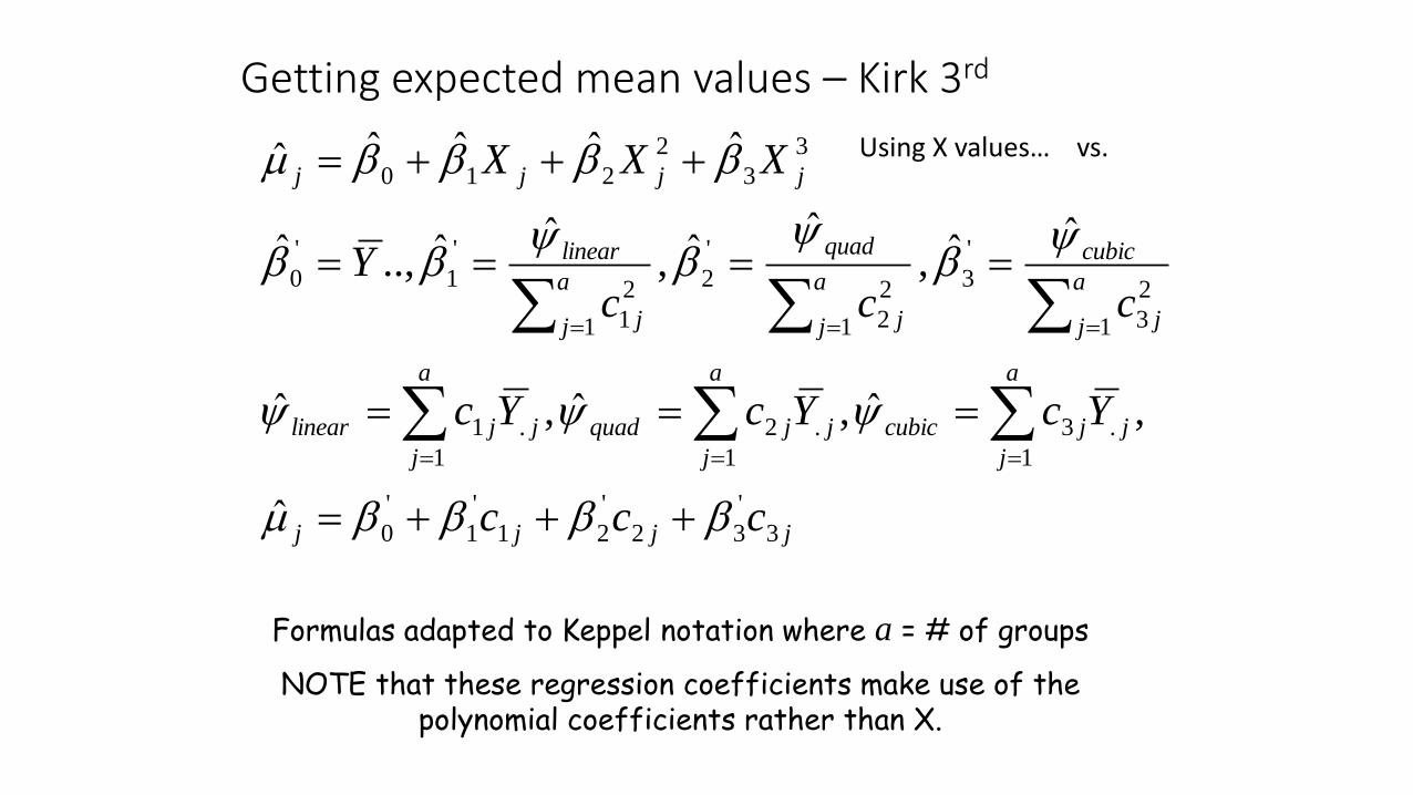
Getting expected mean values – Kirk 3rd
jjjj
a
j
jjcubic
a
j
jjquad
a
j
jjlinear
a
j j
cubic
a
j j
quad
a
j j
linear
jjjj
ccc
YcYcYc
cccY
XXX
3
'
32
'
21
'
1
'
0
1
.3
1
.2
1
.1
1
2
3
'
3
1
2
2
'
2
1
2
1
'
1
'
0
3
3
2
210
ˆ
,ˆ,ˆ,ˆ
ˆˆ,ˆ
ˆ,ˆˆ..,ˆ
ˆˆˆˆˆ
Formulas adapted to Keppel notation where a = # of groups
NOTE that these regression coefficients make use of the polynomial coefficients rather than X.
Using X values… vs.

Holy Week Assignment 8
• Trends Analysis
1. Do a trends analysis on the data in the next slide – see up to what trend is significant
2. Summarize the results in an ANOVA table (complete the table provided)
3. Calculate for the predicted means for each trend component found
4. Plot the predicted means and explain what the analyses and graphs seem to indicate (the plot of the means assuming only a linear trend is provided)

none 10 min 20 min 30 min 40 min 50 min 60 min2 11 8 10 7 10 121 7 8 8 9 13 110 6 10 9 8 9 153 8 7 6 12 11 7
-1 4 8 10 8 5 142 7 5 6 7 9 104 5 6 8 4 8 12
-2 7 6 5 10 10 123 4 9 5 9 8 132 6 5 8 6 7 14
mean 1.4 6.5 7.2 7.5 8 9 12
A Health Center undertook a study to see whether walking more would actually result in significantly more weight loss than walking for shorter periods of time. Seventy volunteers who wanted to lose weight were randomly assigned to one of seven conditions: no walking or walking daily for 10, 20, 30, 40 50, or 60 minutes. The number of pounds lost after a two-week period are indicated in the table above.
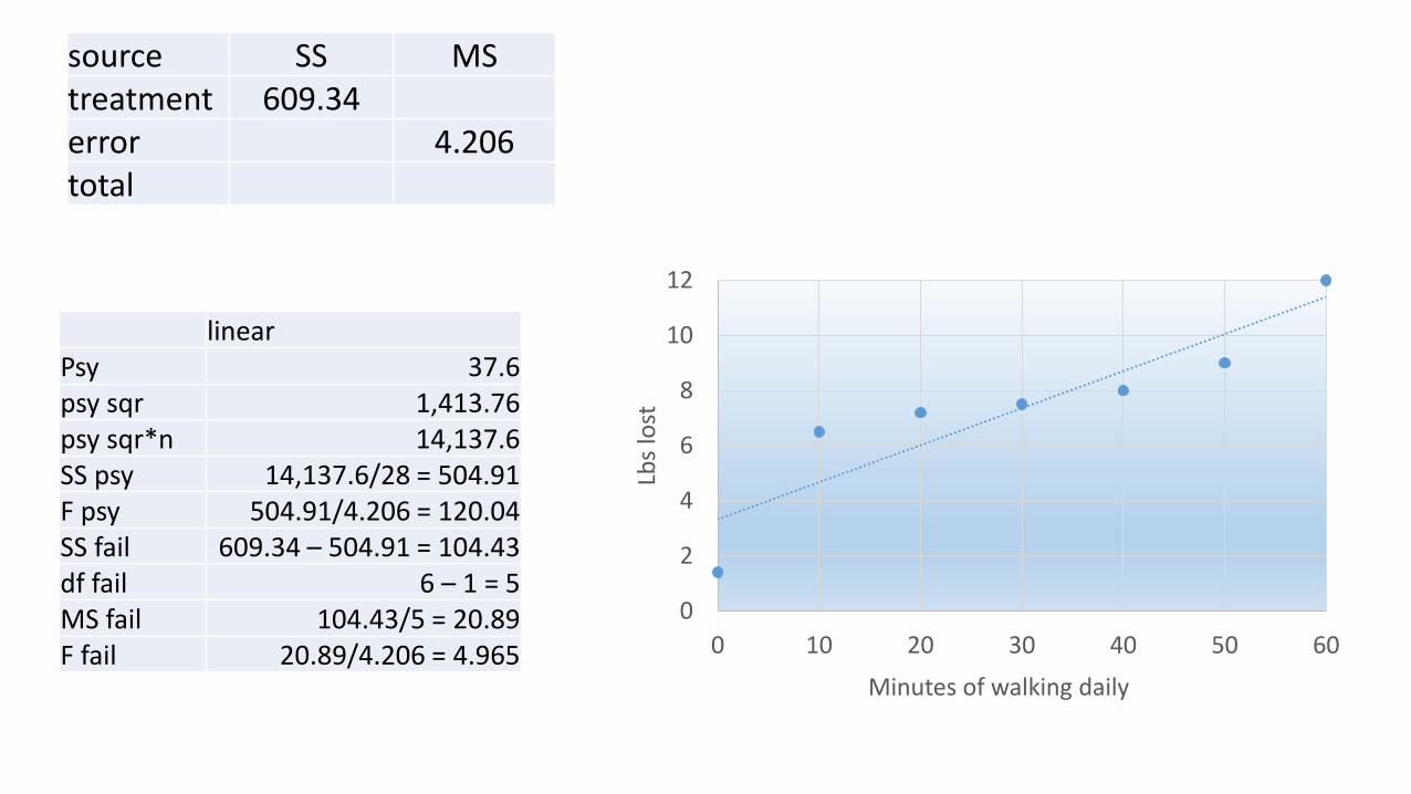
source SS MStreatment 609.34error 4.206total
linearPsy 37.6psy sqr 1,413.76psy sqr*n 14,137.6SS psy 14,137.6/28 = 504.91F psy 504.91/4.206 = 120.04SS fail 609.34 – 504.91 = 104.43df fail 6 – 1 = 5MS fail 104.43/5 = 20.89F fail 20.89/4.206 = 4.965
0
2
4
6
8
10
12
0 10 20 30 40 50 60Lb
s lo
st
Minutes of walking daily

source SS df MS F F crit (.05)treatment 609.343 6 101.557 24.144 2.25
linear 504.914 1 504.914 120.036 4.00failure 104.429 5 20.886 4.965 2.37
quadraticfailure
cubicfailure
error 265 63 4.206total 874.343 69 12.672
Holy Week Assignment 9
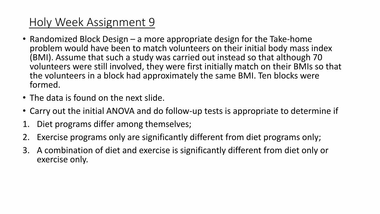
• Randomized Block Design – a more appropriate design for the Take-home problem would have been to match volunteers on their initial body mass index (BMI). Assume that such a study was carried out instead so that although 70 volunteers were still involved, they were first initially match on their BMIs so that the volunteers in a block had approximately the same BMI. Ten blocks were formed.
• The data is found on the next slide.
• Carry out the initial ANOVA and do follow-up tests is appropriate to determine if
1. Diet programs differ among themselves;
2. Exercise programs only are significantly different from diet programs only;
3. A combination of diet and exercise is significantly different from diet only or exercise only.

More appropriate – use a Block design, Subjects matched on BMI prior to random assignment to treatment conditions
block as usual
walking daily 20
min zumba 3Xcount
calories hi protein no carbsbal
diet+walk1 4 10 8 7 10 11 122 -2 5 5 4 5 4 73 -1 7 5 6 5 4 104 0 8 6 7 6 5 115 1 8 6 8 6 6 126 2 9 7 8 8 6 127 2 9 8 9 8 7 138 2 10 8 9 8 7 149 3 11 9 10 9 7 14
10 3 13 10 12 10 8 15

Carrying out follow-up tests for the RB-k design
• Transform the sets of scores for the Block into a single contrast score (much like the Ds in the Two Dependent Samples design)
• Use these contrast scores to calculate for the
• Average contrast score (much like the average D or )
• Standard Error of the observed average contrast score (much like the SED-bar or )
• Calculate for GEM (in this case, a t)
• Check for its significance (df = df residual)
D
DSE