THE CHORE WARS:

HOUSEHOLD BARGAINING AND LEISURE TIME

Leora Friedberg * University of Virginia and National Bureau of Economic Research, lfriedberg@virginia.edu

Anthony Webb

Center for Retirement Research, Boston College, webbaa@bc.edu

December 2005

ABSTRACT Stress over the use of time is a hallmark of American life today. We analyze the role of bargaining in explaining how spouses divide up leisure and chore time. Unlike many other outcomes of household decision-making, time use is easy to observe and to assign to individuals using data from the new American Time Use Survey. Moreover, the ATUS provides a measure of the hourly wage, which we use as a proxy for bargaining power. These factors make for a powerful test of bargaining models. We estimate the effect of a spouse’s relative wages on time use during the weekend, when substitution effects from wages should be much smaller, and controlling for household income, to deal with income effects of wages. We undertake several strategies to isolate the effect of bargaining from that of specialization. We find that, as wives’ relative wages in two-earner households rise, they enjoy significantly more leisure and spend significantly less time doing chores. A one-standard deviation increase in wives’ wage share leads to 18.6 more minutes of total leisure and 14.5 minutes less of chores on a weekend day. While somewhat small relative to total time available, these effects are concentrated in particular leisure activities (especially general relaxing and watching TV) and chores (cooking and cleaning). Wives also spend more time with family members as their relative wages rise, while the reverse is true for husbands. These results hold up when we limit the sample to households in which both spouses work full-time, which reduces potentially confounding influences arising from specialization or non-separability of weekday and weekend time use. The estimated bargaining effects are largest for childless couples, for whom specialization is least likely to be important. * Corresponding author. Department of Economics, University of Virginia, P.O. Box 400182, Charlottesville, VA 22904-4182. 434-924-3177 (phone), 434-982-2904(fax). We are grateful to Dan Hamermesh, Marjorie McElroy, Jay Stewart, Jennifer Ward-Batts, and seminar participants at the National Bureau of Economic Research 2005 Summer Institute and Syracuse University for very helpful comments.

I. INTRODUCTION Stress over the use of time is a hallmark of life today, as made clear by titles from the popular press like “The Overworked American” (Schor 1991) and “The Second Shift” (Hochschild and Machung 1990). Yet, comprehensive American data to shed light on this issue has been lacking until recently. In January 2005, the U.S. Bureau of Labor Statistics released the first year of the American Time Use Survey (ATUS) of 20,000 individuals. Many of the most pressing issues involving time use arise within families – who works and how much, who takes care of children and house, and how do conflicts over these issues get resolved. We use new data on time use to study the impact of household bargaining on the time that spouses spend doing chores and enjoying leisure. Models of household bargaining have two important implications for our understanding of individual welfare. First, the welfare of household members depends on the distribution of bargaining power. Second, household decisions cannot be modeled as the outcome of a single agent maximizing utility. A growing literature offers evidence that bargaining power influences household decisions. Indirect evidence against “unitary” decision-making links variables that are assumed to influence the distribution of bargaining power within the household to household outcomes. These “income-pooling” tests investigate whether the distribution of income between spouses affects outcomes like the amount and allocation of spending on women’s and children’s clothes versus men’s clothes, on alcohol and tobacco, and on food and like children’s well-being.1

Studying time use offers important advantages over earlier tests of income pooling. One difficulty of these tests is finding outcomes that are assignable – that clearly increase the utility of one spouse and not the other. Consumption of most goods is difficult to observe (because we have data on expenditure, not consumption) and to assign (either because it is public in nature or because it is private but observed at the household, not individual level). When the assignability of outcomes is ambiguous, income-pooling tests involve a joint test of household bargaining along with heterogeneity in preferences over outcomes. Time spent on leisure and chores, though, is easy to observe and assign using data from the ATUS. In addition, it is a more interesting outcome in its own right than many of the past studies were able to analyze. Another problem arising in tests of income pooling is observing threat points – utility that spouses would enjoy if they did not cooperate. It has been common to use data on income assignable to a spouse as a proxy for threat points. Absent the availability of interesting natural experiments, though, it is usually difficult to attribute household income other than labor earnings to particular spouses. Studies that analyze earnings require an assumption about separability between labor supply and the outcome being studied.2 An advantage of the ATUS 1 Phipps and Burton (1998), Browning et al (1994), Lundberg, Pollak and Wales (1997), and Ward-Batts (2003) studied clothing spending. Phipps and Burton, Hoddinot and Haddad (1995), and Ward-Batts studied alcohol and tobacco spending. Lundberg, Starz, and Stillman (2003) and Duflo and Udry (2004) studied food spending. Schultz (1990), Thomas (1990), (1994), Haddad and Hoddinott (1994), Rose (1999), Duflo (2003) and Duflo and Udry studied child outcomes like health and education. Friedberg and Webb (2005) use actual data on bargaining power to understand more about the link between determinants and outcomes of household bargaining. 2 Phipps and Burton, Browning et al, and Browning and Chiappori (1999) assume separability between earnings and spending on men’s versus women’s clothing. Lundberg, Starz, and Stillman assume separability between labor

1

in this regard is that it provides a measure of the hourly wage through its link to the Current Population Survey (CPS). Therefore, we can use the hourly wage instead of total earnings as an explanatory variable to proxy for threat points. This eliminates the problem that hours (on the right-hand side) is jointly determined with leisure (on the left-hand side). However, another important problem is heightened when studying time use. The hourly wage affects leisure and housework choices through conventional income and substitution effects, which may be amplified if spouses specialize in working in the market versus working at home in a way that is correlated with their wages. This makes it challenging to isolate the impact of the wage specifically on bargaining power and hence time use. We take a few steps to address these confounding effects. First, we control for total household income in order to deal with income effects. Second, we focus on time use during the weekend and on holidays, when substitution and specialization effects are probably smaller, given that most people concentrate their work hours during the week. Third, we repeat our estimation for various subsamples in which spouses are less likely to be engaging in specialization. Thus, we estimate the extent to which higher-wage spouses consume more leisure and do less housework on typical days off, compared to lower-wage spouses (though the ATUS surveyed one member of each household, so we do not observe time use of people married to each other). Moreover, we focus on individuals in two-earner couples. We do not consider one-earner couples because it is far from clear how bargaining considerations affect labor force participation decisions, and such considerations complicate the already thorny problem of missing wages for non-workers. Consequently, it should be kept in mind that our sample likely includes the people who have the most to gain, in terms of improving their bargaining position, from working. For our sample of respondents in two-earner households, we find statistically significant effects of relative wages on time that women spend enjoying leisure and doing chores. In our preferred specifications, a one standard deviation increase in a wife’s wage raises her total leisure time per weekend day by 18.3 minutes and reduces her total time spent doing chores by 14.5 minutes. While these effects are small relative to total time available in a day, they are larger relative to the time spent in the specific activities in which the effects are concentrated. Women with higher wages spend significantly more time relaxing, watching TV, and with their families. In contrast, men’s overall time use is much less sensitive to relative wages. We observe significant effects for a few male activities, some of them with surprising signs. Men with higher relative wages tend to spend more weekend time engaged in personal non-sleep activities (which includes bathing, grooming, and sex), in exercise and sports, and in fixing things around the house, and they tend to spend less time with their families. The gender-related heterogeneity in estimated bargaining effects suggests that, if our method is valid, it can be used to identify differences in preferences for many specific activities by gender.

force participation and spending on food. Natural experiments provide clean evidence but are limited to particular settings, like the shift in child welfare transfers from fathers to mothers in the U.K. (Lundberg, Pollak, and Wales), the major increase in old age pensions received by blacks in South Africa (Duflo), and the impact of rainfall on crops farmed by men versus women in Côte d’Ivoire (Duflo and Udry).

2

We consider some additional specifications to rule out other explanations. Our results persist when we limit the sample to couples in which both spouses work full-time. This suggests that the estimates do not simply reflect either non-separability between weekday and weekend time use or differences in preferences or household productivity that are correlated with relative wages. Lastly, the effects of relative wages on weekend time use are strongest for childless people, who should be less likely to specialize in a way that is correlated with wages. The rest of this paper is organized as follows. Section II discusses theoretical issues related to time use and household bargaining. Section III describes our data from the new American Time Use Survey. Section IV presents the estimation results, and Section V concludes. II. THEORETICAL CONSIDERATIONS In this section we discuss the theory that will guide the formulation of our empirical specifications, which can be viewed as demand equations for different types of time use. We present, first, a model of time use for individuals that highlights substitution and income effects of wages. Next, we present a non-bargaining model of time use within households that features specialization effects of wages. After that, we discuss models of household bargaining which reveal the bargaining effects in which we are interested. We finish with a discussion of how to identify the bargaining effects of wages on time use. A. Time use decisions of individuals Suppose that an individual has the utility function

U(X, L, C)

where X is consumption of the market-produced good, L is leisure, and C is consumption of household services (chores). The individual also faces the following money, time, and technical constraints:

money budget: Y + wiH = pXX + ∑kmkk Cp

time budget: T = H + ∑kikC~ + L

chores production function: C = ∑∑ == + Kk~k

mk

k~

1kik

ik CC~ω .

Money is derived from non-labor income Y and from working a number of hours H at hourly wage wi, and it is spent on a market-produced good X with price pX and some market-produced services with prices pm

kC k. A fixed time budget T is allocated among work H, some chores ikC~ , and leisure L. Lastly, services produced at home or purchased in the market are added

together to form a composite C, after multiplying time spent on k with a productivity multiplier , which is a shadow or “service wage” for that activity.i

kω3

Assume that X is the numeraire good. This yields the problem of choosing L, i

kC~ , and – how much time to spend on leisure and chores and money to spend on services – to maximize

mkC

3 The same implications will arise from incorporating heterogeneity in disutility of producing or in utility of consuming various services, none of which can be separately identified in our estimation.

3

U(Y+wi(T -∑ ikC~ -L)- , L, ∑ m

kk Cp ∑∑ + mk

ik

ik CC~ω ) .

The first-order constraints governing the production or purchase of household services are

(a) 0UωUwC~

UC

ikX

iik

≤+−=∂

∂ (b) 0UUpCU

CXkmk

≤+−=∂

∂ ,

where UX and UC refer to the partial derivatives of the utility function with respect to X and C. Condition (a) shows that the individual will spend time doing chores when the marginal utility from that effort equals the wage times the marginal utility of the market-produced good X, while condition (b) shows that she will purchase household services when their marginal utility equals their price times the marginal utility of X.4

Combining (a) and (b) yields three possible outcomes for each type of service k:

k is produced at home: (a) met with equality, not (b) ⇒ ik

k

i

ωpw

<

k is purchased in market: (b) met with equality, not (a) ⇒ k

iik p

wω <

k is not consumed: (a), (b) not met with equality ⇒ C

Xi

ik

kU

Uwω

,p1

<

A service will be either purchased or produced when the marginal utility from services is high (relative to that of consuming X and given both its price and the individual’s market and service wages). A particular service will be purchased (produced) when the individual is relatively unproductive (productive) at this chore, given her wage deflated by the price of purchasing the service. We can solve the first-order conditions simultaneously to obtain demand functions for X, L, C that depend on endowments (Y, T ) and real and shadow prices (wi, pk ,ω k). Assuming that all goods are normal, these will yield the following standard comparative static effects of an increase in the individual’s wage w:

1. compensated substitution effect of own wi: ↑ wi ⇒ ↑ H ⇒ ↓ ( iC~ + L) 2. income effect of own wi: ↑ wi ⇒ ↑ L, ↑ X, ↑ C m ⇒ ↓ iC~

Through the compensated substitution effect, the individual will work more, crowding out other uses of time L and . Through the income effect, the individual will consume more of all three goods by purchasing more market goods X and household services C

iC~ m and taking more leisure L;

and as both leisure L and C m rise, time spent on chores will fall. iC~

B. Time use decisions in households without bargaining Incorporating this framework within households adds several complications. In this subsection, we highlight the feature that many services are household public goods – if one spouse spends time on chores, the other benefits. 4 According to the final first-order condition, the individual will choose leisure L such that its marginal utility equals the wage times the marginal utility of market-produced goods which can be purchased with wi.

4

Household benchmark. Consider first the unrealistic case in which a spouse makes exogenous decisions regarding production of household services. We will label these services produced by a spouse (or other family member) and assume that they substitute perfectly for chores done by the individual or purchased in the market. Now, a change in the spouse’s wage w

okC

o affects the spouse’s production of household services as outlined above and yields the following comparative static effects on the individual’s choices:

3. compensated substitution effect of spouse’s wo: ↑ wo ⇒ ↓ Co ⇒ ↑ iC~

4. income effect of spouse’s wo: ↑ wo ⇒ ↑ C m ⇒ ↓ iC~

An increase in o’s wage will lead o to spend less time on chores through the compensated substitution effect, leading i to spend more time on chores. o will spend more money purchasing and less time producing household services through the income effect, with total consumption of C rising under the normal good assumption, so i will spend less time on chores. Thus, the income effect of an increase in one’s own or one’s spouse’s wage is to increase leisure and decrease time spent on chores. The substitution effect of an increase in one’s own wage decreases both leisure and time spent on chores, while the substitution effect of an increase in one’s spouse’s wage decreases one’s own leisure and increases time spent on chores. Specialization. If spouses differ in their market wages and/or service wages (or preferences, though we do not model this), then specialization is Pareto efficient. Consider a social planner maximizing the sum of the spouses’ identical utility functions. The social planner chooses Xi, Lj,

, and for j={i,o} to maximize jkC~ m

kC

V = Ui(Xi, Li, ) ∑∑∑ ++ mk

ok

ok

ik

ik CC~ωC~ω

+ Uo(Y+wi(T - -L∑ ikC~ i)+wo(T - -L∑ o

kC~ o)-Xi-∑ mkk Cp , Lo, ) . ∑∑∑ ++ m

kok

ok

ik

ik CC~ωC~ω

We will focus on the first-order conditions governing choices about services:

(a) 0UwUω2C~

VX

iC

iki

k≤−=

∂∂ (b) 0UwUω2

C~V

Xo

Coko

k≤−=

∂∂

(c) 0UpU2CV

XkCmk

≤−=∂

∂ .

Now, we have four possible outcomes for each type of household service k:

k is produced at home by i: (a) met with equality, not (b), (c) ⇒ ik

k

i

i

ik

o

ok ω

pw ,

wω

wω

<<

k is produced at home by o: (b) met with equality, not (a), (c) ⇒ ok

k

o

o

ok

i

ik ω

pw ,

wω

wω

<<

k is purchased in market: (c) met with equality, not (a), (b) ⇒k

ook

k

iik p

wω ,pwω <<

5

k is not consumed: (a), (b), (c) not met with equality ⇒C

Xo

ok

i

ik

kU2

Uwω

,wω

,p1

< .

More total services will be consumed, compared to the individual’ problem solved earlier, since a given quantity raises utility of both spouses. A particular service will be purchased when both individuals are relatively unproductive at this chore, their wages are relatively high, and the price of the service is relatively low. A service will be produced by a spouse with a relatively high service wage and low market wage, relative to the other spouse wages and the price. The possibility of substitution between spouses in household production increases the scope of the compensated substitution effect of the market wage outlined earlier. Consider the condition

i

ik

k wω

p1

< determining that i, when living alone, will do a particular chore. An increase in i’s

market wage wi may make this condition binding, in which case the service will either be purchased or foregone. In a household with a spouse, there is there is another option – the service may be produced by the other spouse instead of purchased or foregone – reflected in the

additional condition i

ik

o

ok

wω

wω

< , and either condition may become binding as wi rises. This will

make each spouse’s decisions more elastic to wages. Another issue to consider is the possible correlation among wi, wo, ωi, and ωj. For a given person, there is little evidence about the extent to which productivity at market and household work is negatively correlated (a powerful intellect that is rewarded in the marketplace may be negatively correlated with manual dexterity that is productive in the house) or positively correlated (manual dexterity may be productive in both the marketplace and the house). Furthermore, individuals may choose to marry people with negatively correlated skills, which enhances gains from specialization. This would confound identification of a bargaining effect of wages, since specialization could help explain why the lower wage spouse does more chores – though not why the higher wage spouse takes more leisure. However, empirical studies find strong evidence of positive and perhaps growing assortative mating on market wages and education (Winkler 1998). If spouse’s have similar skills, then that reduces the scope for specialization, which reduces concerns about specialization in our empirical analysis. C. Time use decisions in households with bargaining Now, we consider how spouses make joint decisions about the allocation of household resources, including time. At this point, we will ignore the public good aspect of chores, so that they are simply another private good to be bargained over.5 We will not derive the formal properties of individual demand functions, as in McElroy and Horney (1981), but we will simply emphasize the role of threat points. The canonical model of cooperative bargaining developed by McElroy and Horney (1981) and Manser and Brown (1981) assumes that spouses work together to maximize household surplus

5 Adding a public good does not change the qualitative implications of many bargaining models, as long as spouses have different preferences over their consumption or production (Lundberg and Pollak 1996); nor does interdependent utility, as long as spouses do not care excessively for their partners over themselves.

6

and then engage in Nash bargaining over the surplus. In this game, the outcome maximizes the Nash social welfare function N, which is the product of each spouse’s surplus from marriage:

N = (Ui-Ri)*(Uo-Ro),

where Uj and Rj are spouse j’s utility from marriage and reservation utility, or threat point. In the common divorce threat model, the threat point represents utility from divorce.6

As an example, suppose that Uj = Yj, so utility equals one’s share of exogenous household income Y, with Y = Yi+Yo. Then N can be written as N = (Y-Yi-Ro)*(Yi-Ri), and the equilibrium is

Yi = 2

RRY oi −+ ,

subject to Yj ≥ Rj. A general result is that a spouse’s allocation of income increases with non-labor income and their own threat point and decreases with the other spouse’s threat point. Chiappori (1988, 1992) developed an empirical approach to analyze household bargaining without specifying the exact bargaining process. He assumed a Pareto efficient sharing rule φ(wi,wo,Y) that determines the allocation of exogenous income Y, as in the model above, in order to analyze the second stage of decision-making, where each spouse maximizes their individual utility subject to the allocation rule. In the resulting choice problem, individuals make their consumption decisions separately but with Y in an individual’s money budget constraint replaced by φ i, where φ i = Y -φ o represents spouse i’s share of Y. Chiappori (1992) showed that the resulting demand functions depend on φ i instead of Y but otherwise have the same properties as those outlined above. Subsequent work (Browning et al 1994, Browning and Chiappori 1999) tested the model using information on labor market earnings as a “distribution factor” assumed to influence the sharing rule but not other outcomes of bargaining. D. Empirical approach Estimating the effect of bargaining. Our empirical specifications can be viewed as linear demand equations for different types of time use. We will include wage variables to identify the effect of bargaining along with income and demographic variables. The discussion of bargaining supports our assumptions that we can identify the effects of threat points without modeling bargaining itself and using data on wages as a proxy.7 In the simple Nash bargaining game above, each spouses’ threat point enters linearly in the equilibrium allocation, but more complicated utility functions will yield nonlinear effects. Also, we do not know exactly how wages influence threat points. Thus, we will try specifications with linear wages, log wages, and relative wages as approximations of more complicated functional forms. By way of comparison, Bittman et al (2003) undertook a related study using Australian and earlier American data. They estimated the effect of each spouse’s share of income on weekly

6 Lundberg and Pollak (1993) proposed threat points resulting from a non-cooperative game within marriage. Most tests of income pooling, like ours, involve income controlled by spouses whether they are married or divorced and so are unable to distinguish between their model and the standard divorce threat model. 7 Pollak (2005) emphasized that the wage and not labor earnings should be used as a proxy for the threat point, since hours choices are an outcome of the bargaining process.

7

time use, but they did not address many identification issues. We discuss how we deal with these important identification problems next. Income, substitution, and specialization effects. As we outlined above, wages of both spouses affect time use independent of bargaining. We take three steps in the estimation to address confounding income and substitution effects, which may be amplified by specialization. First, we focus on time use during the weekend and on holidays, so we assume that substitution effects then are much smaller when most people in our sample are not working.8 Moreover, the gains from specialization should also be smaller on weekends when time use is less constrained. Second, we control for total household income in order to deal with income effects. However, we recognize that household income is not actually exogenous. It includes not just non-labor income but also earnings and hence work hours H of each spouse. This will induce a mechanical correlation between wages and the left-hand side time use variables – a higher wage, holding household income constant, must imply a reduction in hours of work and hence more time for leisure L and chores Σ iC~ . Moreover, H depends on wages further through the bargaining effect on time use in which we are interested. To deal with these issues, we propose transformations of the wage and household income variables. We will try using spouses’ relative wages, the goal being to isolate the bargaining effect of relative wages while eliminating any mechanical correlation arising because the wage level influences household income and hence time use. We will also try a specification that purges the household income variable of the effects of wages and hours. We do so by regressing household income on both spouses’ wages and usual weekly hours and including the residual as a control variable in the time use regressions.9 This approach addresses the problem that bargaining affects household income via its influence on time use. One last possibility that we will consider is that non-labor income itself might be tainted. Some part of non-labor income may be controlled by one spouse or the other and hence correlated with bargaining power. Also, non-labor income may be endogenously determined by household bargaining (through savings decisions, for example). Lacking a reasonable instrument for non-labor income, we will try a specification that omits it altogether. This specification rests on the assumption, illustrated in the simple Nash bargaining game outlined above, that the threat points that determine the sharing rule are not correlated with the level of household surplus (and income). As it turns out, the specification of the wage variable affects the estimates to some extent, but the specification of the household income variable does not. A third step that we take is to estimate results for limited subsamples in which specialization is less likely. These subsamples include couples in which both spouses work full-time (since they have a demonstrably reduced scope for specialization) and couples with no children (since childbearing is specialized). 8 Based on our idea, Hamermesh (2005) found supporting evidence for this assumption in the ATUS. We show later that higher wages in our sample are associated with more weekday work and less weekend work. 9 As an alternative, we could use the wages and usual weekly hours data to impute household earnings. Because we do not know how well the reported hourly wage captures total cash compensation, nor how well usual weekly hours captures annual hours of work, we prefer the less parameterized approach that we have proposed.

8

Bargaining and labor supply. Another major concern is that labor supply choices may influence threat points. For example, if there are sunk costs of entering the labor force that generate some stickiness in labor supply, it would strengthen the bargaining position of a working over a non-working spouse and influence dynamic labor force participation decisions. Similarly, courts might consider earnings and not just wages in dividing household assets upon divorce, which may favor a non-working over a working spouse. Such considerations have complicate efforts to consider one-earner households in our analysis. First, the current bargaining game may be very different in households where one spouse chose, in an earlier stage of the game, not to work. This suggests that we should not combine one and two-earner households in the same regressions. Second, if it is difficult for a nonworking spouse to exercise the threat of working, then it is not clear how potential market wages relate to a nonworker’s threat point. Third, if the relevant threat point is some function of the potential wage, perhaps discounted for costs of entry, we can offer no useful exclusion restrictions to impute the missing wage, since we take an inclusive approach in considering covariates for our time use regressions. Fourth, if the relevant threat point is close to zero, then we have little to no variation in one spouse’s wage, generating an identification problem in distinguishing the bargaining effect of the other spouse’s relative wage from the effect of household income. Given this host of difficulties, we have chosen to focus exclusively on respondents in two-earner couples. We recognize, nonetheless, that our sample likely includes those individuals who have the most to gain, in terms of improving their bargaining position, from working. Given these considerations, the bargaining effects that we estimate for childless couples may be the cleanest, with observed market wages being most closely aligned to current threat points. Many such couples have not or will not face the more complicated dynamic game that may determine labor supply and subsequent bargaining positions when couples have children. Non-separability. A final identification concern rests on another omitted factor that may explain our results. Time use on weekdays and weekends is not separable – so that a higher-wage spouse who works harder during the week may be more tired and demand more leisure on weekends. Re-estimating the results with the sample limited to households in which both spouses work full-time will help address this concern, along with the possibility noted earlier that wages in part reflect specialization effects. In both cases, the proposed solution is to focus such couples inn which spouses are more likely to be homogeneous in their relative productivity and preferences across activities. Our main results continue to stand in this specification, though there are some differences in estimated effects of wages on specific activities. In sum, we assume that the relative strength of spouses’ threat points determines the split of household surplus and in turn time use. The resulting prediction that we seek to test is that the higher one’s wage, relative to one’s spouse’s, the more of the marital surplus that one will enjoy, which translates into spending more time in leisure and less time doing chores. We will analyze this prediction for individuals in two-worker couples, and we will consider various specifications of the wage and household income variables.

9

III. DATA A. The American Time Use Survey The U.S. government has only recently begun to produce a survey of time use for a large nationally representative sample. A random sample of civilian non-institutionalized households leaving each month’s Current Population Survey (CPS) are chosen to participate in the American Time Use Survey (ATUS), and an adult is randomly sampled from each household to be surveyed about their time use in a single 24-hour period. A day of the week is pre-assigned to each person, with oversamples of weekend days. People are contacted for eight consecutive weeks on the day following their pre-assigned day of the week in order to secure the interview. The first year of ATUS data covers 2003. The overall response rate in the ATUS was 57%, yielding a sample of 20,720 respondents. According to the ATUS documentation, “the primary reason for nonresponse is that the designated persons are tired from participating in the CPS survey” (p.10, American Time Use Survey User’s Guide). Of obvious concern is that the busier respondents are, the less likely they are to take time to respond to the ATUS. We present evidence below that this does not appear to generate any systematic bias in our results. Abraham et al (2005) found that observed characteristics likely to be correlated with busyness – like usual weekly hours of work and presence of children – had little effect on response rates. Much of the ATUS sample of 20,720 is not suitable for our analysis, such as respondents who were not married, who had other adults besides their spouse or disabled adults in the household, and who did not have wage data for themselves or their spouses from the CPS. We undertook the following restrictions to arrive at the sample that we analyze:

1. We eliminated households of individuals or cohabiting couples (resulting in a sample of 9,550). Cohabiting couples might make decisions differently than married couples. 2. We eliminated households with any member other than the married couple who was over the age of 16 (resulting in 9,176), since other adults might contribute time and/or money to the household and thus alter the time use of respondents. 3. We eliminated households in which a member recorded in the ATUS was not recorded in the CPS, since we need CPS data for other household members (resulting in 8,850). 4. We eliminated households not already eliminated in #3 in which the ATUS respondent was reported as unmarried in the CPS, since we need wage data on both spouses from the CPS (resulting in 8,744). 5. We eliminated households not already eliminated in #2 in which the household was reported as containing a subfamily in addition to the main family (resulting in 8,736). 6. We eliminated households in which either spouse was reported as disabled in the CPS or ATUS, since time use decisions in such households may be very different (resulting in 8,287).10

7. We eliminated households in which the ATUS respondent could not account for more than 30 minutes of their daily activities, indicated by a Tier 1 code of 50 (resulting in 7,669). 8. We focus on respondents in two-worker households (resulting in a sample of 3,965).11

10 We use information from both the ATUS and the CPS on disability (defined by whether it makes someone unable to work). Disability reported at the time of the ATUS was more current but not defined as uniformly as in the CPS, particularly for the spouse. 11 This is defined by whether the respondent was employed and at work (TELFS=1) and whether the spouse was employed (TESPEMPNOT==1). Information on whether the spouse was at work is not reported.

10

9. We focus on respondents for whom we could compute non-missing non-zero values for the hourly wage for both spouses using CPS data (resulting in 2,804).12

10. Of those respondents, 1,434 were interviewed about time use on weekends or holidays, consisting of 685 male respondents and 749 female respondents. B. Measuring time use ATUS interviewers recorded every activity done during the assigned day, categorized by type of activity, start and stop time, location, and presence of others. We classified every household activity in one of four categories: leisure (L), chores (C), work (H), and emergencies (E). For the most part, we followed the ATUS in grouping activities. We made slight changes to the ATUS definitions of some activities, but the estimation results presented below were not sensitive to these distinctions. We exclude emergencies in most of our analysis below, since they add noise and probably tell us little about regular time use patterns Our classification of activities is summarized below and detailed in the Appendix. Leisure: • Personal care, sleep • Volunteer activities • Eating, drinking (including as part of job) • Phone, mail, e-mail with family, friends • Socializing, relaxing, leisure (same) • Education (if “for personal interest”) • Sports, exercise, recreation (same) • Personal care services • Religious, spiritual activities • Associated travel Chores: • Household activities • Professional services • Caring for, helping household, non- • Household services household members • Government services • Consumer purchases • Associated travel Work: • Working, work-related activities • Associated travel • Education (if “for degree”) Emergencies and other exclusions: • Personal care emergencies • Activities that cannot be coded • Obtaining police, fire services • Associated travel • Civic obligations

12 The hourly wage is computed as usual weekly earnings divided by usual weekly hours. The same information appears again in the ATUS for the respondent but not the spouse, so we use the older CPS data for both. Those whose usual weekly hours varied were assigned a value of 40 if they reported in a follow-up question that their usual hours were full-time or 20 if they reported part-time or (in two cases) varying. Of the 3,965 respondents remaining after step #8, 13 had a value of zero for their own or their spouse’s usual weekly earnings and hence the wage; 468 respondents had a missing value for usual earnings; 429 had a missing value for the spouse’s usual earnings; and 251 had missing values for both; resulting in the 2,804 respondents remaining after step #9.

11

C. Measuring other covariates The ATUS reports a great deal of data obtained from the outgoing CPS survey, which took place 2-5 months earlier. We use wage data, computed as either hourly earnings if reported, or weekly earnings divided by usual weekly hours of work. The CPS also reports household income data collected in the fifth month of the survey and grouped in 16 categories; in most specifications we include dummy values for each range value. Time use will also depend on the number and age of children in the household. More children, especially young ones, means more time or money is required for childcare, while older children may help with household chores. Therefore, it is important to control for the presence and age of children; we also try estimating regressions separately by presence and age of children. Lastly, we will control for education, race, age, and season of the year. IV. RESULTS We estimate OLS regressions of the determinants of time spent in leisure L and producing household services C on weekends and holidays. Our sample consists of individuals in two-worker households. We estimate all specifications separately for men and women, since their time use patterns appear very different. Our hypothesis is that the higher a spouses wage is, the more time they enjoy in leisure and the less time they spend doing chores. A. Raw statistics Table 1 shows characteristics of the estimation samples, consisting of working men and women who have working spouses and wage data for both and who were surveyed on weekends or holidays. Men have higher wages than women, with average hourly wages of 21.76 and 16.77, respectively. The average hourly wage of their spouses is almost identical, at 17.41 for wives of male respondents and 21.49 for husbands of female respondents, while the modal range of household income was $75,000-99,999. The average age of respondents is just over 40, again with almost identical means for respondent vs. spouse husbands and wives. The fact that wives of male respondents look a great deal like female respondents, and the same for husbands of female respondents, substantially reduces concerns about sample selection bias. As we noted earlier, response rates could depend on busyness and hence wages. We might expect less busy, and hence lower-wage, people to respond more readily, and specialization suggests that their spouses would be relatively busier and higher-wage. The symmetry that we just noted yields evidence against this source of bias. Table 2 shows general time use patterns of our sample of weekend respondents, compared to weekday respondents selected according to the same criteria. In general, men spend more time working and less time doing chores on both weekdays and weekends compared to women, while men have less leisure time on weekdays and more on weekends than women do. On weekend days, men (women) work an average of 108 (84) minutes, take leisure of 1059 (1023) minutes, and do chores for 272 (331) minutes.13 The extra time available for leisure and chores on the weekends is 420 minutes for men and 327 minutes for women. 13 All of these gender differences in aggregate time use are statistically significant.

12

Table 2 also reports detailed time use within these broad categories, according to classifications in Appendix Table 2. Weekend leisure consists of, roughly, over 500 minutes of sleeping, 86 minutes of eating, around 20 minutes (for women) and 40 minutes (for men) of sports and exercise, and around 30 minutes of religious and volunteering activities. Men spend another 330 minutes and women around 280 minutes in general relaxation and leisure. This broad category breaks down into 120 minutes (for women) and 180 minutes (for men) watching TV, a little under 60 minutes socializing with family and friends, 20 minutes reading and writing, and around 15 minutes each of attending social events and arts/entertainment events. Chores can be grouped into three major types – doing work around the house, taking care of people, and shopping. We grouped work around the house as either “women’s” chores (cooking, cleaning, laundry, household organization) or “men’s” chores (repairs and maintenance inside and outside, lawn and garden, working on vehicles and appliances) as an easy shorthand, and also based on observed patterns. Women spend 144 minutes on “women’s” chores on weekend days, while men spend 57 minutes on “women’s” chores. Conversely, women spend only 27 minutes on “men’s” chores and men spend 86 minutes. Women spend more time than men caring for household members (63 vs. 45 minutes) and shopping (79 vs. 66 minutes). Almost everyone in our sample has some positive amount of time allocated to the broad categories of leisure and chores. In other regressions, we will focus on much narrower activities for which some or many people report zero time spent. Some of the same issues about the treatment of these zeroes arises in using short-term expenditure data to study consumption (cf. Ward-Batts 2003). Some zeroes are generated by people who are completely uninterested in the activity, as explained by the inequality restrictions in the model we presented earlier (which we view as applying to average time use over an interval like a month). Other zeroes are generated because people did not participate in an activity on that particular day, while over a longer period they do. A tobit would be appropriate for the “non-participant” model, but OLS is consistent for the “infrequent participant” model. We will present OLS estimates, but ultimately we will discuss tobit results as well. B. Estimation results, overall time use In this subsection, we discuss different specifications of the wage and household income variables and then the estimated effects in our preferred specification. Various specifications for women (Table 3). The left hand side variable in Table 3 is total minutes spent by women taking leisure (top panel) and doing chores (bottom panel). The table reports key coefficient estimates from different specifications of the wage and household income variables. Estimates that are statistically significant at a level of 90% or better are outlined in dashed boxes. Estimated effects of the other independent variables (children, education, age, race, season) change little across these specifications and will be discussed later as part of the main specification. Higher relative wages significantly raise women’s leisure time and reduce their chore time across the specifications in Table 3. Column (1) includes linear controls for own hourly wage wi, spouse’s wage wo, and household income dummies. The coefficient of own wage on leisure time

13

is 2.99 (0.73), implying that each dollar raises the average women’s leisure time by 2.99 minutes per weekend day, while a one standard deviation increase of $11.20 raises it by 33.6 minutes.14

Column (2) controls instead for the individual’s wage share oi

i

www+

, the own wage divided by

the sum of the own plus spouse’s wage. Here, bargaining will be identified purely from the individual’s share of the household’s total earnings potential, while all level effects of wages will be absorbed by household income. This specification results in a statistically significant and somewhat smaller effect of relative wages than in column (1). This may confirm our concern about a mechanical positive correlation between wage levels and leisure, since a higher wage with constant household income requires a decline in hours of work. The coefficient estimate of 146.5 (57.8) on the wage share implies that a one standard deviation increase of 0.139 will raise wives’ leisure time by 20.4 minutes per weekend day. We will say more about the magnitude of the estimated effects when we discuss the main specification shortly. Notably, the estimates jump by a few minutes if we control separately in column (3) for the sum of wages, which is the denominator of the wage share variable.15 The total wage raises leisure significantly by 1.3 minutes per dollar, while it has a smaller and insignificant negative effect on chores. The specifications in columns (4) and (5) keep the wage share while using transformations of household income. The estimated effect of wages remains almost the same, but the R2 declines. Column (4) replaces household income dummies with residual household income, which is meant to capture non-labor income after regressing household income on both spouses’ wages and usual weekly hours. This has an insignificant effect on leisure time and a significant (and wrong-signed) positive effect on chore time.16 Column (5) omits household income entirely. Very similar changes in the wage variable occur across the specifications in the lower panel of Table 3, where the left-hand side variable is minutes spent on chores. Given the similarities of the results between across the last four columns, we have chosen column (2) as our preferred specification for the rest of the paper. Preferred specification for men and women (Table 4). Table 4 reports the results from the specification taken from column (2) in Table 3 (and repeated here), with left-hand side variables of leisure and chore time for men and women. The effects of relative wages are statistically significant and of the expected sign for women, as noted earlier. The coefficient estimate of 146.5 (57.8) implies that a 10 percentage point increase in a woman’s wage share raises her leisure time by 14.65 minutes per weekend day. A one standard deviation increase in the wage

14 The magnitudes of the estimated effects are very similar if we control for logs instead of levels of wages, but the R2 is lower. Friedberg and Webb (2005) found that wives’ earnings have a greater direct effect on reported bargaining power than husbands’ earnings do in the Health and Retirement Study. 15 Arguably, education is pre-determined in relation to wages, so it may yield better identification of bargaining effects. However, if we control for an individual’s “education share” (defined using highest completed grade in the same way as wages), it is often wrong-signed and insignificant, with or without including the wage share. This parallels Friedberg and Webb (2005), who found that relative education did not affect reported bargaining power, although relative earnings did. 16 A one standard deviation increase in residual household income (of 17.1 thousand dollars) raises time spent on chores per weekend day by 19.8 minutes.

14

share (which, for example, would move it from a mean of 0.441 to 0.580) raises it by 20.4 minutes, while shifting her wage share from 25% to 75% raises it by 73.3 minutes. The estimated coefficient on the wage share on women’s chore time is -108.5 (56.1).17 This implies that a one standard deviation increase in a woman’s wage share is expected to reduce her time spent doing chores by 13.6 minutes per weekend day, while shifting her wage share from 25% to 75% raises it by 54.3 minutes. While a negative correlation between skill in market and home production could explain why lower wage wives do more chores through specialization rather than bargaining, it would not explain why higher wage wives take more leisure, since specialization would lead them to work more. The estimated effects for men are very small and wrong-signed, so, on the whole, bargaining affects men’s time use much less than women’s.18 However, we find great variety in the impact of relative wages on time spent in specific activities and with family members, including some significant effects for men, in results that we will discuss shortly. A few other covariates have significant effects. Household income dummies in Table 4 are jointly significant but exhibit absolutely no clear monotonic pattern.19 Children, especially younger ones, significantly reduce parents’ and raise chore time (which includes child care). Children under the age of 6 reduce leisure time by 60-80 minutes per weekend day (and more so for women), while children aged 6 and over reduce leisure time by 40-45 minutes.20

Own and spouse’s education have some significant but non-monotonic effects, and we do not know whether they act as another proxy for bargaining power or reflect heterogeneity in time use preferences. Men who did not finish high school take significantly more leisure and their wives take less, while women with postgraduate degrees take less leisure and their husbands take less as well. Race has significant effects for men but not women.21 Black men take significantly and substantially more leisure (93.6 minutes per weekend day) and do less chores (46.6 minutes), as do black women but with smaller and insignificant estimated effects. Other non-white non-black men do significantly less chores (73.5 minutes), while non-white non-black women take less

17 The estimated effects of covariates on leisure versus chores need not be equal in absolute value because there are other categories of time use (work and emergencies), for which we report results in Table 5. 18 When we used seemingly unrelated regression for leisure and chores, the estimated standard errors fell by a few minutes or less. When we used quantile regression, we found that estimated effect of the wage share on wives’ leisure time declines a little, while the effect on wives’ chore time intensifies a little, at higher quantiles of the wage share. 19 For example, being in the modal household income category of $75,000-99,999 has very small and statistically insignificant effects on average time use. 20 When households include kids under the age of 6, men spend 81.8 minutes more on child care and 59.3 minutes less on leisure, on average (controlling for everything else reported in Table 4), with little change in time devoted to other chores or work; women spend 110.0 minutes more on child care, 81.0 minutes less on leisure, and 21.5 minutes less on other chores. When households include kids aged 6 and over, men spend 22.2 minutes more on child care, along with 29.2 minutes more on other chores and 43.0 less on leisure; women devote 29.0 minutes more to child care, 10.7 minutes more (though this amount is not statistically significant) to other chores and 45.3 less to leisure. While the R2 of the regression is a little lower if we control for number rather than presence of kids, doing so suggest that each child under the age of 6 reduces mothers’ and fathers’ leisure time by 56.3 and 37.6 minutes, respectively, while each child aged 6 and over reduces it by 22.1 minutes and 21.0 minutes. 21 Spouse’s race did not have a statistically distinguishable effect from own race.

15

leisure and do more chores, but not significantly so. Older husbands reduce leisure time and raise chore time for both spouses by 2-3 minutes for each year of age, while older wives have the opposite effect, raising leisure and reducing chores time of both spouses by a similar amount. C. Estimation results, specific activities (Table 5) We find great variety in how relative wages influence time spent in specific activities and with family members. The significant bargaining effects are concentrated in a few areas, and some of them are quite important in magnitude relative to average time spent in such activities. Moreover, these effects differ by gender, and some are surprising. The revealed heterogeneity shows that we can use the estimated bargaining effects to identify differences in preferences between men and women for many specific activities. Table 5 estimates the same specification as Table 4, reporting only the coefficient on the wage share, with many different categories of leisure and chores on the left-hand side. We will judge these results by the magnitude of the estimated coefficients, while noting that they lose some precision as the focus narrows. Work and emergencies. Table 5 begins by reporting the estimated effects of the wage share on aggregate time spent working and on emergencies, in addition to results for leisure and chores that were shown previously. Notably, the wage share has small and highly insignificant effects on time spent working. When we go back to the specification with each spouse’s wage entered linearly so as to test for substitution effects, the effects of own wages on time spent working are negative (that is wrong-signed) for both men and women, while the effects of spouses’ wages are negative (and right-signed) but small and insignificant.22 These results support our assumption that substitution effects of wages are not of concern on weekends. The effects of the wage share on time spent in emergencies are negative and very small with large standard errors, so it seems reasonable to separate such activities from the others that we consider. Types of leisure. Next, Table 5 reports the estimated effects of the wage share on particular types of leisure and chores.23 The interesting effects for women’s leisure are concentrated in the “general leisure” category, while other categories like sleeping, eating (whether at home or away), exercise, and religious activities are unresponsive. Recall as a baseline that the estimated effect of the wage share on total leisure time is 146.5 (57.8). The estimated effect on all subcategories will sum to that total (though small ones are in fact omitted from Table 5). In comparison, the estimated effect on the subcategory of “general leisure” is bigger, at 167.9

22 With time spent working on the left-hand side, the estimated coefficients on own and spouse’s wages are -1.10 (0.95) and -1.06 (0.75) for men and -1.17 (0.56) and -0.60 (0.56) for women If we control for own and spouse’s industry, occupation, and class of job, the effects of wages on work time move closer to zero for men but more negative for women. If we distinguish between paid work done out of the house versus at home, the coefficients on own and spouse’s wages for men are -1.71 (0.89) and -0.87 (0.72) for the former versus 0.61 (0.36) and -0.19 (0.28) for the latter. Thus, we have evidence of a significant but very small substitution effect of own wages on doing paid work at home (with a one standard deviation gain raising men’s time spent working at home by 7.0 minutes); but in contrast, the coefficient on own wage remains negative for women doing paid work at home and away. 23 The estimated effects of any particular covariate on subcategories will add up to equal the estimated effect for the entire category. However, we omitted minor categories of time use in Table 5, all of which appear in Table 2. We will consider estimating tobits instead of linear regressions for these narrowly defined categories; preliminary estimates show that this does not alter the statistical significance of the wage effects that are of interest.

16

(47.6), so that a one standard deviation increase in wage share raises time spent on this activity by 23.4 minutes. This represents 8.3% of the average 280 minutes spent on “general leisure” and, to look at it another way, explains 13.2% of each standard deviation of 177 minutes. Table 5 further breaks down this effect on “general leisure” into coefficients of 25.3 (28.4) on socializing and spending time at home with family and friends, 30.6 (20.7) on going out for arts and entertainment, and 94.8 (38.2) on “relaxing and leisure”. This last subgroup can be broken down yet again into 27.6 (14.0) on relaxing, thinking, doing nothing, and smoking and 73.6 (35.0) on watching TV – so that a one standard deviation increase in the wage share raises time spent in these activities by 37.8% and 7.9%, respectively. While aggregate leisure time of men is not affected by the wage share, a few specific activities are. The wage share has an effect of 31.4 (13.1) on non-sleep personal care (which includes grooming, bathing, and sex). This implies a 12.4% increase for a one standard deviation increase in the male wage share. While the coefficient of 37.9 (33.3) on time spent participating in sports and exercise is not significant here, it is in some later specifications. Types of chores. For reference, the estimated effect of the wage share on aggregate time spent by women doing chores is -108.5 (56.1). As shown in Table 5, this consists of -91.2 (38.6) for “women’s” chores and -23.9 (17.9) for “men’s” chores, countered by positive but insignificant effects on caring for household and non-household members. The effect of a one standard deviation increase in the wage share on “women’s chores” is a -8.9% reduction. Among “women’s” chores, the coefficients are -45.8 (30.1) for cleaning, -26.6 (18.8) for food preparation, and -18.8 (15.1) for household organization and other tasks; some of these effects are statistically significant in later specifications. Again, aggregate chore time for men is not affected by the wage share, but there are a few strong effects on specific activities which move in unexpected directions. In the expected direction and not that small but insignificant is the estimated effect on time spent shopping for goods of -46.9 (29.4) (with an almost significant coefficient of -15.7 (9.7) on shopping for food and -29.6 (26.0) on shopping for other than food and gas). Unexpectedly, the estimated effect of the wage share on time spent doing “men’s” chores is positive and fairly large, at 51.3 (39.9), which breaks down to 52.9 (21.8) for repairs and maintenance inside the house and 22.3 (24.0) for lawn and garden work, but -21.3 (22.4) for repairs and maintenance outside the house. A one standard deviation increase in the male wage share raises total time spent on “men’s” chores by 8.4% of the average and time spent on repairs and maintenance in the house by 38.5%. We may infer that men like to spend time doing such activities.24 In contrast, the estimated effect on time spent caring for household children is negative, at -25.7 (22.0). Later on, some significant negative effects of the male wage share on time spent with children emerge. Time spent with family. Now, we consider time spent with particular family members, rather than time spent engaged in specific activities. The “who” information reported at the end of Table 5 was collected for all activities except work, sleep, grooming, and “personal activities”

24 If we add a control for home ownership, it has a statistically significant effect but almost no impact on the estimated wage share effects. It might be desirable to control for home ownership in order to capture wealth effects, but on the other hand home ownership may be an outcome of bargaining.

17

(sex, using the bathroom, etc.). As the wage share shifts from men to women, spouses spend significantly more time together. The estimated effect of a woman’s wage share on time spent with husbands is 138.6 (72.9), so a one standard deviation increase raises it by 19.3 minutes, or 4.7%, and the effect of a man’s wage share on time spent with wives is -62.0 (84.1). We find later that these effects are stronger for full-time working couples and especially for couples with no children. This is the only evidence we can provide that spouses influence the activities of one another directly, rather than reacting to the others’ decisions as in noncooperative bargaining. Regarding children, as relative wages of women rise, they spend a little more time with their children but less time providing secondary child care. As relative wages of men rises, they spend considerably less time with their children at all. We find later that these effects vary substantially with the age of the child. Conclusions. We conclude that bargaining generally has more of an effect on women’s weekend time use than on men’s. As wives’ wages increase relative to their husbands’, they spend more time relaxing, watching TV, and with their husbands and less time engaged in “women’s” chores. At the same time, as husbands’ wages rise, they spends more time in personal grooming and fixing things inside the house and spend less time with their families. The effects are substantial in some categories of time use, and the overall effects are important if the marginal utility of leisure is relatively steep. D. Estimation results, specific subsamples In this subsection, we report additional specifications and robustness checks. First, we try to rule out other explanations for our results. We find many similar or stronger bargaining effects on specific categories of time use when we focus on those individuals who work full-time and whose spouses work full-time. This suggests that the estimates do not simply reflect specialization or non-separability between weekday and weekend time use. We also find that the effects of relative wages on aggregate weekend time use are strongest for childless people, but significant effects on some specific activities arise for those with children as well. Sample of full-time workers (Tables 6, 7). It is possible that people who work harder during the week (and have a higher wage share) are simply more tired and less productive at household chores on the weekend – so that time use on weekdays and weekends is not separable. We tried two different approaches to deal with this concern. In Table 6, we limited the sample to people in households with both spouses working full-time (35 hours or more per week) in the CPS, as opposed to working at all. Another purpose of limiting the sample in this way is to focus on spouses who are more homogeneous in their market work and therefore less likely to be engaging in specialization in household work. In this sample, the estimated wage share effects on women’s overall time use are somewhat smaller, at 107.5 (80.7) for leisure time and -76.3 (74.7) for chore time. Yet, the notable effects of relative wages on specific activities from Table 5 remain largely unchanged or stronger in Table 6, though standard errors have risen for the smaller sample. The overall decline in the wage share effect is concentrated in other activities that remain statistically insignificant.

18

For example, the declines for women’s leisure activities are greatest for spending time with family and friends and for engaging in sports and exercise. However, the effect of the wage share on men’s personal non-sleeping time and on women’s “general leisure” hardly changed, while the effect on relaxing/ thinking/doing nothing grew substantially from 27.6 (14.0) to 57.7 (22.6). The reduced coefficient for chores is driven by moderate but, again, statistically insignificant increases in the coefficients on taking care of household children and on shopping. Yet, the estimated effect on time spent doing “women’s” chores remained almost unchanged; and within this category the coefficient on cleaning dropped, while the coefficient on cooking jumped from -26.6 (18.8) to -59.2 (27.7) and became significant. Lastly, Table 6 shows how estimates of time spent with family members change when we limit the sample. Many of the wage share effects became more extreme, positive for women and negative for men. For example, the coefficient on spending time with spouses rose from 138.6 (72.9) to 173.8 (103.1) for women. The only exception is that the coefficients on secondary child care dropped for both but especially for women, from -56.9 (65.9) to -126.1 (85.4). In Table 7, we try another approach by going back to the full sample of working spouses and including a control for each spouse’s usual weekly hours from the CPS. It has little effect on the estimated wage share coefficients, changing them from 146.5 (57.8) to 165.4 (60.0) for women’s weekend leisure time and from -108.5 (56.1) to -96.0 (57.9) for women’s chore time. In sum, while the effects of the wage share on aggregate leisure and chore time of women fell when we limited the sample to both spouses working full-time, the declines occurred in categories that remain insignificant, and most of the significant effects on specific activities stayed the same or grew bigger. These results do not support alternate hypotheses about specialization or non-separability of weekend and weekday time use. Weekday time use. Our results for the more homogenous sample discussed above help to rule out the possibility that productivity or preferences for market versus home production are negatively correlated. Another way to address concerns about unobservable heterogeneity – that women with higher wage shares and men with lower wage shares have systematically different preferences for time use – is to compare weekend with weekday estimates. These results are reported in Table 8. The wage share has a much smaller and insignificant effect on women’s leisure time on weekdays than on weekends, while it has a large positive effect on time working (suggesting a strong substitution effect) and a large negative effect on time spent doing chores. The coefficients for particular weekday activities are substantially different in Table 8 than for weekends in Table 5, and they remain small across all types of leisure activities. Meanwhile, the wage share now has large and statistically significant negative, instead of positive, effects on time spent with family members. Also of note, the positive effect of wage share on time men spend on interior repairs and maintenance does not appear on weekdays. Thus, most of the effects of the wage share are quite different during the week. The large negative effect of the wage share on women’s time doing chore, which is what makes way when high wage-share women spend more time working, is concentrated in “women’s” chores and in caring for household children. We cannot completely rule out the hypothesis that heterogeneity in preferences and household productivity explain the weekend results, since

19

women with higher wage shares do less cooking and cleaning on both weekdays and weekends; but the major differences in most of the wage share effects, especially on leisure, suggest that heterogeneity in preferences are not driving the key results. Heterogeneity involving children. Another set of results addresses heterogeneity related to the presence and age of household children. The scope for specialization by childless couples is much more limited, compared to childbearing and childrearing. In fact, the bargaining effects that we estimate are strongest for childless people, but significant effects on some specific activities arise among those with children as well. In Table 9 we divide the sample into respondents with children under the age of 6, with children but none under the age of 6, and without any children. We report results for aggregate time use and for a small subset of specific activities – those for which the coefficient estimate was at least as large as the standard error. For respondents with small children, shown in the first set of results, the coefficient for women’s leisure time remains similar at 136.1 (88.8), but the coefficient on women’s chores becomes positive and highly insignificant. The estimated coefficient for “general leisure” remains significant but falls to 124.0 (71.9), with substantial declines for relaxing and doing nothing and for watching TV, but with an increase for socializing with family and friends from 25.3 (28.4) to 61.5 (47.8). The coefficient on men’s chore time remains insignificant but is substantially more negative, at -130.0 (116.3); this change is diffused across many types of chores. Lastly, the wage share has a much greater effect on some of the “who” categories. The effect on time spent with the spouse falls for men from -62.0 (84.1) to -179.0 (168.3) and rises for women from 138.6 (72.9) to 232.6 (121.7), which is now statistically significant. The effect is even greater for time spent with her children, rising to 363.4 (117.7) overall and 183.1 (124.6) for secondary child care, the only positive result in that category. Applying the same metric as we did earlier, a one-standard deviation increase in the wage share raises time spent with children by 50.6 minutes. For respondents without small children but with children aged 6 and over, the coefficient of the wage share on women’s leisure time is inconsequential, but the coefficient on women’s chore time reaches -164.7 (110.1). Men now have significant positive effects of the wage share on some of their leisure activities (socializing with family and friends and participating in sports and exercise). And in sharp contrast, a woman’s wage share has negative effects on spending time with children while a man’s has positive effects on spending time with spouses. Both have large negative effects of the wage share on secondary child care, reaching -238.8 (171.1) for men and -244.5 (171.4) for women. Lastly, the wage share has major, highly significant effects on time use of childless respondents – with these effects again observed for wives and not husbands. The coefficient on women’s total leisure time is 261.6 (85.2) and on women’s total chores time is -180.3 (78.7), so a one standard-deviation increase in the wage share results in 36.4 more minutes of leisure and 25.1 minutes less of chores. It has very substantial effects on women’s time watching TV, with a coefficient of 201.2 (61.0), and doing “women’s” chores, at -106.0 (56.6). And, as the wage share shifts from women to men, it substantially increases time that spouses spend together, with a coefficient of 235.0 (125.1) for women. A further breakdown shows that these effects are entirely concentrated (and are even bigger) among couples in which wives are over the age of 40 (with the one standard-deviation effects on leisure and chores reaching 42.7 and 28.8 minutes).

20

As we discussed earlier, labor supply decisions and bargaining outcomes may be part of a simultaneous game. However, this seems like less of a concern for childless couples, since children impose strong constraints on time use and involve considerable specialization. It is possible, then, that the bargaining effects that we estimate for childless couples are not only the strongest – and specifically appear for couples older than childbearing age – but the “cleanest”. The results also indicate the possibility of important dynamics involved with bargaining, since wage effects shift as children are born and age. V. CONCLUSIONS A growing literature offers evidence that the distribution of bargaining power within a household influences household spending decisions. Studying the allocation of leisure and chore time between spouses offers important advantages over the previous research. Time use is easy to observe and assign using data from the new American Time Use Survey. Also, the ATUS provides a measure of the hourly wage through its link to the Current Population Survey. Using the hourly wage instead of total earnings as a proxy for threat points eliminates the problem that hours (on the right-hand side) is jointly determined with leisure (on the left-hand side). In our estimates we control for household income to deal with income effects of wages and study time use on weekends, when substitution effects from wages appear to be much smaller. We find that, as wives’ wages in two-earner households rise, wives enjoy significantly more leisure – especially general relaxing and watching TV – and spend significantly less time doing chores – especially cooking and cleaning. A one standard deviation increase in a wife’s wage raises her total leisure time per weekend day by 18.3 minutes and reduces her total time spent doing chores by 14.5 minutes. Women with higher wages also spend significantly more time with their families. We observe significant effects for a few male activities, some of them with surprising signs. Men with higher relative wages tend to spend more weekend time engaged in personal non-sleep activities (which includes bathing, grooming, and sex), in exercise and sports, and in fixing things around the house, and they tend to spend less time with their families. These results show that we can use this approach to identify differential preferences for specific activities by gender. We consider some additional specifications to rule out other explanations, and we find considerable heterogeneity in bargaining effects by presence and age of children. One way to extend this line of research would be to find exogenous variation in threat points to provide identification from something other than own wages. Some possibilities include cross-state variation in policies involving welfare benefits, divorce laws, child support enforcement laws, and many others discussed in McElroy (1990).25 Besides that, it may be possible to use this data to understand more about how bargaining is related to the determination of labor supply.

25 This possibility is currently limited by the short time period that the ATUS covers. As a prelude to such an analysis, the results for women in Table 4 get stronger (with larger coefficients and no increase in standard errors) when we include dummies for U.S. state of residence. These dummies are jointly statistically significant in explaining leisure but not chores.

21

APPENDIX Appendix Table 1 shows how we classified time use activities into the following categories: Leisure (L), Chores (C), Work (H), and Emergencies (E). The table lists ATUS activities in the order in which they are classified and, by way of comparison, their official grouping into ATUS classifications (American Time Use Survey User’s Guide 2004 pp.41-42).

APPENDIX TABLE 1 Classification of ATUS activities

ATUS code Description Our classification ATUS classification

01 except … personal care L 0105 personal care emergencies E personal care

02 except … household activities C household activities 020903 020904 household & personal mail,

messages, & e-mail L telephone calls, mail, & e-

mail 0299 household emergencies E household activities 03 care for & help household

members C caring for & helping

household members 04 care for & help non-household

members C caring for & helping non-

household members 05 except … work & work-related activities H 050201-050203 socialize, eat, sports as part of job L

working & work-related activities

06 except ... educational activities H or L 060101 060301 060401

education “for degree” H

060102 060302 060402

education “for personal interest” L educational activities

07 consumer purchases C 08 except ... professional & personal care svcs C 0805 personal care services L 09 household services C 10 except ... government services & civic

obligations C

100101 100301 use, wait to use police & fire svcs E

purchasing goods & services

1002 100303 do, wait to do civic obligations & participation

E organizational, civic, & religious activities

11 eat & drink L eating & drinking 12 socialize, relax, & leisure L 13 sports, exercise, & recreation L leisure & sports

14 religious & spiritual activities L 15 volunteer activities L

organizational, civic, & religious activities

16 except ... telephone calls C 160101 160102 telephone calls w/ family, friends L

telephone calls, mail, & e-mail

17 travel assigned to associated activities above 50 data codes E other activities, n.e.c.

22

Notes: • We follow the ATUS in grouping travel with the activity for which the travel took place. We assigned travel that was not associated with a particular activity to adjacent activities. • We follow the ATUS in distinguishing household and personal mail, messages, and e-mail from other household activities. While the ATUS groups them in a category with telephone calls, we group all such communications with friends and family as Leisure and other communications as Household services. • We follow the ATUS in grouping “consumer purchases”, “professional and personal care services”, “household services”, and most subcategories of “using government services” together as part of Household services. The ATUS distinguishes “civic obligations and participation” from other categories of “using government services” and groups that with religious and volunteer activities; we group it with Emergencies. We classify using “police and fire services” as part of Emergencies as well. • We group educational activities, which the ATUS keeps distinct, as part of either leisure or work, depending on whether the activities are identified as being “for personal interest” or “for degree”. Whenever one or the other of several codes that make this distinction appeared, other educational activities were attributed to the same category. • We ignored information on the length of time that the last activity continued into the following 24-hour period. In many of our estimation results, we broke down leisure and chores into finer categories according to the following classification:

APPENDIX TABLE 2 Subclassification of ATUS activities classified as Leisure and Household services

ATUS code Description

Leisure activities 0101 Personal care – sleep 01, except 0101 0105 0805

Personal care – other (grooming, sex)

11 Eating & drinking 020903 020904 160101 160102

General leisure – mail, e-mail, phone w/ family, friends

1201 General leisure – socializing, spending time w/ family, friends 1202 General leisure – attending social events 120301 120302 General leisure – relaxing & leisure – relaxing, thinking, doing

nothing, smoking, taking drugs 120303 120304 General leisure – relaxing & leisure – watching TV 120307 120308 General leisure – relaxing & leisure – games, computer use 120312 120313 General leisure – relaxing & leisure – reading, writing other 1203 General leisure – relaxing & leisure – other (music, hobbies) 1204 General leisure – going out for arts & entertainment other 12 General leisure – other (waiting associated with 1301 130301 130401 Sports, exercise, & recreation – participating

23

other 13 Sports, exercise, & recreation – watching, other 14 Religious & spiritual activities 15 Volunteering

Chores 0201 “Women’s” chores – cleaning 0202 “Women’s” chores – food preparation 020902 020999 0305 “Women’s” chores – laundry, household organization, helping

household adults, other 0203 020905 “Men’s” chores – fixing things inside (interior maintenance &

decoration, home security) 0204 020502 “Men’s” chores – fixing things outside (exterior maintenance &

decoration, pool & hot tub) other 0205 “Men’s” chores – lawn & garden 0207 0208 “Men’s” chores – cars, tools, appliances (repair & maintenance) 020901 Household finances 0301 Caring for household members – children – general (physical care,

reading, playing, talking, attending children’s events) 0302 160103 Caring for household members – children – educational 170301 Caring for household members – children – driving 0303 0399 Caring for household members – children – other (children’s health) 0206 Caring for household members – pets 0304 Caring for household members – caring for other adults 0401 0402 0403 Caring for non-household members – children 0405 Caring for non-household members – other adults – helping 170402 170499 Caring for non-household members – other adults – driving 0404 0499 Caring for non-household members – other adults – caring, other 070101 070103 170701 Shopping – for goods – food 070102 Shopping – for goods – gasoline other 07 1707 Shopping – for goods – food 0801 09 160106 160107

Shopping – for household services (childcare, cleaning, lawn services, pet care, home maintenance)

other 08 16 10 as noted above

Shopping – for other services (professional services, government services, phone calls with sales people & other service providers)

REFERENCES Abraham, Katherine, Aaron Maitland, and Suzanne Bianchi. 2005. “Nonresponse in the American Time Use Survey: Who is Missing from the Data and How Much Does It Matter?” Manuscript, University of Maryland. American Time Use Survey User’s Guide 2004. Bureau of Labor Statistics and U.S. Census Bureau. November 2004. Bittman, Michael, Paula England, Liana Sayer, Nancy Folbre, and George Matheson. 2003. “When Does Gender Trump Money? Bargaining and Time in Household Work.” American

24

Journal of Sociology 109 (1): 186-214. Browning, Martin, Francois Bourguignon, Pierre-André Chiappori, and Valérie Lechene. 1994. “Income and Outcomes: A Structural Model of Intrahousehold Allocation.” Journal of Political Economy. 102 (6): 1067-96. Browning, Martin, and Pierre-André Chiappori. 1994. “Efficient Intra-Household Allocations: A General Characterisation and Empirical Tests.” Econometrica. 66 (6): 1241-1278. Chiappori, Pierre-André. 1988. “Rational Household Labor Supply.” Econometrica 56: 63-89. Chiappori, Pierre-André. 1992. “Collective Labor Supply and Welfare.” Journal of Political Economy 100: 437-467. Duflo, Esther. 2003. “Grandmothers and Granddaughters: Old Age Pension and Intra-Household Allocation in South Africa.” World Bank Economic Review 17 (1): 1-25. Duflo, Esther, and Christopher Udry. 2004. “Intrahousehold Resource Allocation in Cóte d’Ivoire: Social Norms, Separate Accounts and Consumption Choices.” National Bureau of Economics Research Working Paper No. 10498. Friedberg, Leora, and Anthony Webb. 2005. “An Empirical Investigation of Household Bargaining.” Draft, University of Virginia. Haddad Lawrence, and John Hoddinott. 1994. “Women’s Income and Boy-Girl Anthropometric Status in the Cóte d’Ivoire.” World Development 22 (4): 543-553. Hamermesh, Daniel. 2005. “Why Not Retire? The Time and Timing Costs of Market Work.” Manuscript, University of Texas at Austin. Hochschild, Arlie Russell, and Anne Machung. 1990. “The Second Shift.” Avon Books, paperback edition. Hoddinott, John and Lawrence Haddad. 1995. “Does Female Income Share Influence Household Expenditures? Evidence from Cóte d’Ivoire.” Oxford Bulletin of Economics and Statistics 57(1): 77-96. Lundberg, Shelly, and Robert Pollak. 1993. “Separate Spheres Bargaining and the Marriage Market.” Journal of Political Economy 101 (6): 988-1010. Lundberg, Shelley, and Robert Pollak. 1996. “Bargaining and Distribution in Marriage.” Journal of Economic Perspectives 10 (4): 139-158. Lundberg, Shelley, Robert Pollak, and Terence Wales. 1997. “Do Husbands and Wives Pool Resources: Evidence from the UK Child Benefit.” Journal of Human Resources 32 (3): 463-480.

25

Lundberg, Shelley, Richard Starz, and Steven Stillman. 2003. “The Retirement Consumption Puzzle: A Marital Bargaining Approach.” Journal of Public Economics 87 (5-6): 1119-1218. Manser, Marilyn, and Murray Brown. 1980. “Marriage and Household Decision Making: A Bargaining Analysis.” International Economic Review 21: 31-44. McElroy, Marjorie. 1990. “The Empirical Content of Nash-Bargained Household Behavior.” Journal of Human Resources 25 (4): 559-583. McElroy, Marjorie and Mary Horney. 1981. “Nash-Bargained Decisions: Toward a Generalization of the Theory of Demand.” International Economic Review 22 (2): 333-349. Phipps, Shelley, and Peter Burton. 1998. “What’s Mine is Yours? The Influence of Male and Female Incomes on Patterns of Household Expenditure.” Economica 65: 599-613. Pollak, Robert. 2005. “Bargaining Power in Marriage: Earnings, Wage Rates and Household Production.” National Bureau of Economic Research Working Paper No. 11239, April. Rose, Elaina. 1999. “Consumption Smoothing and Excess Female Mortality in Rural India.” Review of Economics and Statistics 81 (1): 41-49. Schor, Juliet. 1991. The Overworked American: The Unexpected Decline of Leisure. Basic Books. Schultz, T. Paul. 1990. “Testing the Neoclassical Model of Family Labor Supply and Fertility.” Journal of Human Resources 25 (4): 599-634. Thomas, Duncan. 1990. “Intra-Household Resource Allocation: An Inferential Approach.” Journal of Human Resources 25 (4): 635-664. Thomas, Duncan. 1994. “Like Father, Like Son, Like Mother, Like Daughter: Parental Resources and Child Height.” Journal of Human Resources 29 (4): 950-988. Ward-Batts, Jennifer. 2003. “Out of the Wallet and into the Purse: Using Micro Data to Test Income Pooling.” Claremont Colleges Working Paper No. 2003-10. Winkler, Anne. 1998. “Earnings of Husbands and Wives in Dual-Earner Families.” Monthly Labor Review 121 (4): 42-48.

26

TABLE 1 Sample means and standard deviations

Men Women

hourly wage 21.76 (11.60) 16.77 (11.20) spouse’s hourly wage 17.41 (10.60) 21.49 (12.35) household income [modal answer] $75,000-99,999 $75,000-99,999 hourly wage . (own + spouse’s hourly wage)

0.557 (0.139) 0.441 (0.139)

any kids age < 6 0.302 0.303 any kids age ≥ 6 0.455 0.450 self spouse self spouse education: didn’t finish high school 0.053 0.044 0.031 0.064 high school diploma 0.242 0.247 0.262 0.267 some college 0.295 0.307 0.327 0.290 Bachelor’s degree 0.276 0.269 0.247 0.238 post-graduate 0.134 0.134 0.134 0.142 age 42.6 (10.1) 40.5 (9.8) 40.4 (10.0) 42.2 (10.1) race: white 0.874 0.925 black 0.088 0.041 other nonwhite 0.038 0.033 hispanic 0.072 0.092 season: winter 0.277 0.271 spring 0.255 0.220 summer 0.215 0.276 fall 0.253 0.232 sample size N 685 749

Data from the 2003 American Time Use Survey. This table reports statistics on the independent variables included in regressions reported in later tables. Standard deviations are reported in parentheses for variables that are not binary. Sample selection criteria are described in detail in the text. The sample includes non-disabled married individuals who work, whose non-disabled spouses work, who have earnings data from the CPS, and who were interviewed on the weekend or on a holiday. Variables are defined as follows. The hourly wage is defined using CPS data as usual weekly earnings divided by usual weekly hours, with more detail reported in the text. Household income is recorded in the discrete CPS variable HUFAMINC, merged into the ATUS. Age, gender, and kid variables are defined using ATUS roster data; education, race, and ethnicity variables are defined using CPS data merged into the ATUS. Season is defined based on the month of the year in which the respondent was surveyed by the ATUS.

27

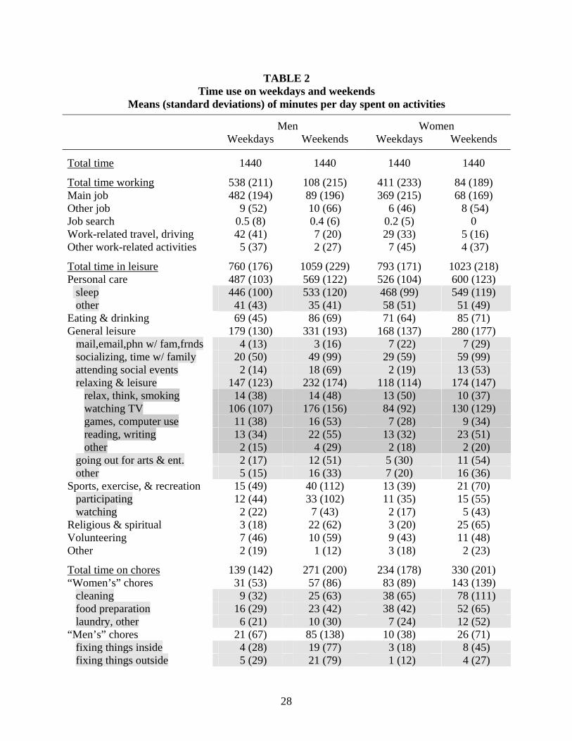
TABLE 2 Time use on weekdays and weekends

Means (standard deviations) of minutes per day spent on activities

Men Women Weekdays Weekends Weekdays Weekends

Total time 1440 1440 1440 1440

Total time working 538 (211) 108 (215) 411 (233) 84 (189) Main job 482 (194) 89 (196) 369 (215) 68 (169) Other job 9 (52) 10 (66) 6 (46) 8 (54) Job search 0.5 (8) 0.4 (6) 0.2 (5) 0 Work-related travel, driving 42 (41) 7 (20) 29 (33) 5 (16) Other work-related activities 5 (37) 2 (27) 7 (45) 4 (37)

Total time in leisure 760 (176) 1059 (229) 793 (171) 1023 (218) Personal care 487 (103) 569 (122) 526 (104) 600 (123) sleep 446 (100) 533 (120) 468 (99) 549 (119) other 41 (43) 35 (41) 58 (51) 51 (49) Eating & drinking 69 (45) 86 (69) 71 (64) 85 (71) General leisure 179 (130) 331 (193) 168 (137) 280 (177) mail,email,phn w/ fam,frnds 4 (13) 3 (16) 7 (22) 7 (29) socializing, time w/ family 20 (50) 49 (99) 29 (59) 59 (99) attending social events 2 (14) 18 (69) 2 (19) 13 (53) relaxing & leisure 147 (123) 232 (174) 118 (114) 174 (147) relax, think, smoking 14 (38) 14 (48) 13 (50) 10 (37) watching TV 106 (107) 176 (156) 84 (92) 130 (129) games, computer use 11 (38) 16 (53) 7 (28) 9 (34) reading, writing 13 (34) 22 (55) 13 (32) 23 (51) other 2 (15) 4 (29) 2 (18) 2 (20) going out for arts & ent. 2 (17) 12 (51) 5 (30) 11 (54) other 5 (15) 16 (33) 7 (20) 16 (36) Sports, exercise, & recreation 15 (49) 40 (112) 13 (39) 21 (70) participating 12 (44) 33 (102) 11 (35) 15 (55) watching 2 (22) 7 (43) 2 (17) 5 (43) Religious & spiritual 3 (18) 22 (62) 3 (20) 25 (65) Volunteering 7 (46) 10 (59) 9 (43) 11 (48) Other 2 (19) 1 (12) 3 (18) 2 (23)

Total time on chores 139 (142) 271 (200) 234 (178) 330 (201) “Women’s” chores 31 (53) 57 (86) 83 (89) 143 (139) cleaning 9 (32) 25 (63) 38 (65) 78 (111) food preparation 16 (29) 23 (42) 38 (42) 52 (65) laundry, other 6 (21) 10 (30) 7 (24) 12 (52) “Men’s” chores 21 (67) 85 (138) 10 (38) 26 (71) fixing things inside 4 (28) 19 (77) 3 (18) 8 (45) fixing things outside 5 (29) 21 (79) 1 (12) 4 (27)

28

lawn & garden 8 (36) 34 (83) 5 (29) 12 (47) cars, tools, appliances 4 (29) 12 (44) 1 (7) 1 (10) Household finances 2 (10) 3 (30) 3 (18) 2 (13) Caring for household members 45 (79) 46 (93) 77 (98) 62 (100) children 41 (79) 42 (92) 71 (98) 55 (99) general 30 (69) 37 (83) 51 (75) 48 (88) educational 4 (17) 2 (14) 6 (21) 2 (12) driving 6 (16) 3 (16) 12 (24) 4 (16) other 1 (9) 1 (14) 2 (17) 2 (20) pets 4 (13) 4 (17) 4 (14) 7 (24) caring for other adults 1 (9) 0.1 (3) 1 (14) 0.4 (5) Caring for non-hhold members 9 (39) 12 (50) 13 (54) 17 (60) children 2 (15) 3 (21) 5 (33) 5 (31) other adults 8 (37) 9 (46) 8 (43) 12 (51) helping 4 (26) 6 (38) 2 (16) 5 (35) driving 3 (17) 2 (13) 3 (17) 4 (19) caring, other 1 (10) 1 (17) 3 (30) 2 (21) Shopping 30 (58) 64 (96) 47 (72) 78 (97) goods 23 (48) 60 (94) 36 (63) 74 (95) household services 1 (10) 1 (15) 2 (12) 1 (10) other 5 (26) 3 (18) 9 (30) 3 (17) Other 2 (24) 4 (23) 2 (11) 3 (24)

Total time in emergencies 2 (24) 2 (15) 2 (9) 2 (15)

Total time spent ... With family members 231 (169) 535 (266) 308 (203) 564 (252) household 217 (159) 515 (266) 286 (195) 531 (261) non-household 14 (71) 20 (78) 22 (77) 33 (107) With spouse 166 (146) 437 (266) 172 (161) 408 (260) spouse only, no one else 100 (128) 193 (218) 97 (129) 186 (222) With any kids 113 (142) 297 (289) 187 (204) 324 (299) own household kids 106 (139) 273 (291) 172 (200) 291 (304) providing secondary child care to own kids < age 13

94 (147) 272 (311) 155 (208) 284 (316)

With friends 14 (60) 45 (124) 22 (72) 43 (120)

N 662 685 708 749

Data from the 2003 American Time Use Survey. Each column reports the time use of a different sample from the ATUS. Time use is reported in average minutes per day. Standard deviations are reported in parentheses. Sample selection criteria are described in detail in the text. The sample includes non-disabled married individuals who work, whose non-disabled spouses work, who have earnings data from the CPS. The classification of time use is described in the Appendix. “Leisure, redefined” and “chores, redefined” begin with the definitions of leisure and chores reported in Appendix Table 1 and switch the categories “caring for household children” and “‘men’s’ chores” from chores to leisure.

29

TABLE 3 Impact of wages on women’s minutes per day in leisure, chores on weekends

OLS regression results for selected variables, preliminary specifications

Dependent variable: Minutes of leisure per day on weekends and holidays

Selected independent variables (1) (2) (3) (4) (5)

hourly wage wi 2.99 (0.73) - - - - spouse’s hourly wage wo -0.39 (0.74) - - - -

- 146.5 (57.8) 153.3 (57.6) 140.2 (58.1) 150.6 (58.3) wage share oi

i

www+

total wage wi+wo - - 1.27 (0.50) - - household inc dummies? [p-value on joint F test]

yes [0.0749]

yes [0.1706]

yes [0.0408]

no no

residual hhold inc (000’s) - - - -0.495 (0.500) - residual squared - - - 0.018 (0.020) -

R2 0.0999 0.0914 0.0984 0.0800 0.0737

Dependent variable: Minutes of chores per day on weekends and holidays

hourly wage wi -1.77 (0.69) - - - - spouse’s hourly wage wo 0.94 (0.72) - - - -

- -108.5 (56.1) -110.6 (56.2) -108.2 (55.5) -113.2 (55.6)wage share oi

i

www+

total wage wi+wo - - -0.38 (0.48) - - household inc dummies? [p-value on joint F test]

yes [0.0000]

yes [0.0000]

yes [0.0000]

no no

residual hhold inc (000’s) - - - 1.235 (0.455) - residual, squared - - - -0.005 (0.016) -

R2 0.1139 0.1109 0.1116 0.0860 0.0725

Data from the 2003 American Time Use Survey. Each column reports results from a separate regression, differing by the specification of the covariates reported in the table. The sample consists of non-disabled married women who work, whose non-disabled husbands work, and who have earnings data from the CPS. Specific sample selection criteria are described in the text. N = 749. The dependent variable in each regression in the upper and lower panels is, respectively, minutes of leisure or chores per day on weekends and holidays. Additional covariates are the same as those in Table 4. Huber-White standard errors are reported in parentheses. Coefficient estimates in cells that are outlined with dashes are statistically significant at the 90% level or higher. Variables are defined in Table 1. The classification of time use is described in the Appendix.

30

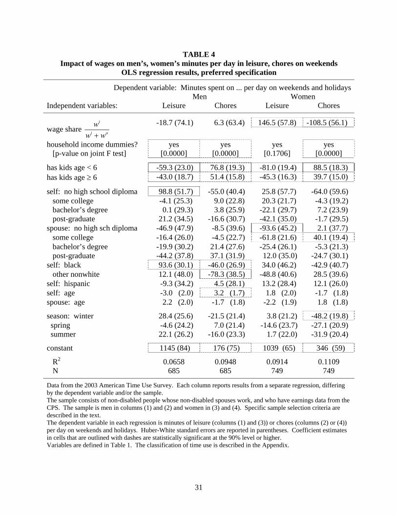
TABLE 4 Impact of wages on men’s, women’s minutes per day in leisure, chores on weekends

OLS regression results, preferred specification

Dependent variable: Minutes spent on ... per day on weekends and holidays Men Women Independent variables: Leisure Chores Leisure Chores

-18.7 (74.1) 6.3 (63.4) 146.5 (57.8) -108.5 (56.1) wage share oi

i

www+

household income dummies? [p-value on joint F test]

yes [0.0000]

yes [0.0000]

yes [0.1706]

yes [0.0000]

has kids age < 6 -59.3 (23.0) 76.8 (19.3) -81.0 (19.4) 88.5 (18.3) has kids age ≥ 6 -43.0 (18.7) 51.4 (15.8) -45.3 (16.3) 39.7 (15.0)

self: no high school diploma 98.8 (51.7) -55.0 (40.4) 25.8 (57.7) -64.0 (59.6) some college -4.1 (25.3) 9.0 (22.8) 20.3 (21.7) -4.3 (19.2) bachelor’s degree 0.1 (29.3) 3.8 (25.9) -22.1 (29.7) 7.2 (23.9) post-graduate 21.2 (34.5) -16.6 (30.7) -42.1 (35.0) -1.7 (29.5) spouse: no high sch diploma -46.9 (47.9) -8.5 (39.6) -93.6 (45.2) 2.1 (37.7) some college -16.4 (26.0) -4.5 (22.7) -61.8 (21.6) 40.1 (19.4) bachelor’s degree -19.9 (30.2) 21.4 (27.6) -25.4 (26.1) -5.3 (21.3) post-graduate -44.2 (37.8) 37.1 (31.9) 12.0 (35.0) -24.7 (30.1) self: black 93.6 (30.1) -46.0 (26.9) 34.0 (46.2) -42.9 (40.7) other nonwhite 12.1 (48.0) -78.3 (38.5) -48.8 (40.6) 28.5 (39.6) self: hispanic -9.3 (34.2) 4.5 (28.1) 13.2 (28.4) 12.1 (26.0) self: age -3.0 (2.0) 3.2 (1.7) 1.8 (2.0) -1.7 (1.8) spouse: age 2.2 (2.0) -1.7 (1.8) -2.2 (1.9) 1.8 (1.8)

season: winter 28.4 (25.6) -21.5 (21.4) 3.8 (21.2) -48.2 (19.8) spring -4.6 (24.2) 7.0 (21.4) -14.6 (23.7) -27.1 (20.9) summer 22.1 (26.2) -16.0 (23.3) 1.7 (22.0) -31.9 (20.4)

constant 1145 (84) 176 (75) 1039 (65) 346 (59)

R2 0.0658 0.0948 0.0914 0.1109 N 685 685 749 749

Data from the 2003 American Time Use Survey. Each column reports results from a separate regression, differing by the dependent variable and/or the sample. The sample consists of non-disabled people whose non-disabled spouses work, and who have earnings data from the CPS. The sample is men in columns (1) and (2) and women in (3) and (4). Specific sample selection criteria are described in the text. The dependent variable in each regression is minutes of leisure (columns (1) and (3)) or chores (columns (2) or (4)) per day on weekends and holidays. Huber-White standard errors are reported in parentheses. Coefficient estimates in cells that are outlined with dashes are statistically significant at the 90% level or higher. Variables are defined in Table 1. The classification of time use is described in the Appendix.

31

TABLE 5 Impact of wages on minutes per day in specific activities on weekends

OLS regression results, coefficient on wage share, specification from Table 4

Dependent variable: Minutes spent on various activities per day on weekends and holidays

Coefficient on wage share Men Women

Total time working 14.9 (68.8) -31.7 (50.8)

Total time in leisure -18.7 (74.1) 146.5 (57.8) [ 20.4, 2.0%]

Total time on chores 6.3 (63.4) -108.5 (56.1) [-15.1, -4.6%]

Total time in emergencies -2.5 (3.6) -6.2 (5.8)

Types of leisure Personal care -1.4 (38.1) -20.5 (32.6) sleep -32.8 (35.9) -23.2 (30.8) other 31.4 (13.1) [ 4.4, 12.4%] 2.7 (14.0) Eating & drinking -7.7 (19.4) -6.3 (18.4) General leisure -11.9 (61.0) 167.9 (47.6) [ 23.4, 8.3%] mail, e-mail, phone w/fam,friends -0.7 (7.2) 3.2 (7.2) spend time w/ family, friends 27.0 (30.4) 25.3 (28.4) attending social events 3.6 (19.9) 3.2 (13.4) relaxing & leisure -42.3 (49.7) 94.8 (38.2) [ 13.2, 7.6%] relaxing, thinking, smoking 2.1 (12.0) 27.6 (14.0) [ 3.8, 37.8%] watching TV -5.3 (43.9) 73.6 (35.0) [ 10.2, 7.9%] games, computer use -0.7 (17.9) -0.0 (9.1) reading, writing -31.0 (20.0) -2.5 (13.6) going out for arts & entertainment 4.1 (15.5) 30.6 (20.7) Sports, exercise, & recreation 23.0 (36.0) -8.6 (18.7) participating 37.9 (33.3) -12.5 (14.9) watching -15.1 (12.8) 4.0 (11.5) Religious & spiritual -26.3 (23.0) 1.7 (16.5) Volunteering 8.5 (17.4) 15.4 (15.2)

Types of chores “Women’s” chores -12.5 (28.2) -91.2 (38.6) [-12.7, -8.9%] cleaning -11.3 (19.4) -45.8 (30.1) food preparation -6.2 (13.6) -26.6 (18.8) household organization, other 4.9 (7.4) -18.8 (15.1) “Men’s” chores 51.3 (39.9) -23.9 (17.9) fixing things inside 52.9 (21.8) [ 7.4, 38.5%] -13.2 (11.2) fixing things outside -21.3 (22.4) -10.3 (7.1) lawn & garden 22.3 (24.0) -1.3 (12.3) cars, tools, appliances -2.6 (12.7) 0.9 (2.9) Household finances 28.0 (27.3) -2.6 (4.2)

32

Caring for household members -22.2 (24.8) 10.4 (24.1) children -23.9 (24.3) 12.3 (23.4) general -25.7 (22.0) 17.8 (21.0) educational -3.5 (4.9) -0.4 (4.0) driving 1.9 (4.5) -2.4 (4.2) pets 1.2 (4.2) -2.0 (5.4) other adults 0.5 (0.4) 0.1 (1.3) Caring for non-household members 3.9 (14.6) 16.0 (16.3) children 2.6 (7.7) -2.4 (9.9) other adults 1.3 (12.7) 18.4 (13.3) caring 4.7 (4.1) 1.4 (5.2) helping -0.0 (10.8) 8.7 (9.2) driving -3.5 (3.2) 5.6 (4.6) Shopping -40.2 (30.5) -8.8 (25.9) for goods -46.9 (29.4) -8.6 (25.6) food -15.7 (9.7) -6.7 (8.6) gasoline -1.7 (1.3) -0.0 (0.6) other -29.6 (26.0) -2.0 (24.2) for household services 1.7 (4.0) 4.1 (2.6) for other services 5.0 (9.9) -4.3 (4.2)

Total time spent ... with family members -84.2 (82.8) 178.6 (65.4) [ 24.9, 4.4%] household -93.0 (82.1) 153.8 (69.5) [ 21.4, 4.0%] non-household 8.7 (30.6) 24.8 (28.1)

with spouse -62.0 (84.1) 138.6 (72.9) [ 19.3, 4.7%] with spouse only, no one else 15.8 (57.4) 147.3 (54.1) [ 20.5, 11.0%]

with any kids -105.5 (70.8) 31.6 (61.9) with own household kids -65.5 (66.8) 21.8 (59.2) providing secondary child care to own kids < age 13

-94.8 (71.3) -56.9 (65.9)

with friends -30.8 (35.4) -3.6 (31.4)

N 685 749

Data from the 2003 American Time Use Survey. Each cell reports the coefficient estimate and standard error on the wage share, obtained from separate regressions that differ by the dependent variable. The dependent variable in each regression is minutes spent on specific activities or with specific people per day on weekends and holidays. All other details are the same as those in Table 4. Huber-White standard errors are reported in parentheses. Coefficient estimates in cells that are outlined with dashes are statistically significant at the 90% level or higher. The classification of time use is reported in the Appendix. Information on the presence of others was not collected for the following activities: sleeping, grooming, personal activities, and work.

33

TABLE 6 Impact of wages on weekend time use, sample in which both spouses work full-time

OLS regression results, specification from Table 4

Dependent variable: Minutes spent on various activities per day on weekends and holidays

Coefficient on wage share Men Women

Total time working 17.4 (91.3) -32.7 (66.7)

Total time in leisure -36.5 (96.0) 107.5 (80.7)

Total time on chores 18.3 (84.6) -76.3 (74.7)

Types of leisure Personal care – other 36.4 (16.1) 14.7 (17.4) General leisure 1.8 (81.1) 169.9 (64.6) socialize, spend time w/ family, friends 36.6 (42.4) -0.6 (36.5) attending social events 12.7 (32.7) 13.4 (16.6) relaxing & leisure -83.3 (65.6) 89.1 (56.9) relaxing, thinking, smoking 14.6 (13.7) 57.7 (22.6) watching TV -14.1 (64.1) 62.6 (55.2) Sports, exercise, & rec – participating 85.1 (56.2) -40.0 (25.7)

Types of chores “Women’s” chores 39.1 (38.9) -93.4 (52.9) cleaning 16.0 (27.3) -27.2 (37.9) food preparation 11.2 (19.2) -59.2 (27.7) “Men’s” chores 40.2 (57.5) -15.5 (22.9) fixing things inside 87.8 (35.3) -6.8 (14.8) lawn & garden -11.0 (36.9) -6.8 (16.3) Caring for household members – children -40.6 (31.7) 26.4 (33.2) Shopping – for goods -29.3 (44.3) 8.4 (36.0)

Total time spent … with family members – household -56.2 (108.8) 173.5 (95.2) with spouse -88.7 (114.0) 173.8 (103.1) with any kids -122.9 (87.4) 59.0 (81.1) with own household kids -52.1 (83.0) 53.1 (77.1) provide 2ndary child care to own kids < 13 -104.9 (93.3) -126.1 (85.4)

N 450 470

Data from the 2003 American Time Use Survey. Each cell reports the coefficient estimate on the wage share, obtained from separate regressions that differ by the dependent variable. The specifications are the same as in Table 5 and 6, except the sample here is restricted to full-time workers (those with usual weekly hours of 35 or more). Huber-White standard errors are reported in parentheses. Coefficient estimates in cells that are outlined with dashes are statistically significant at the 90% level or higher.

34

TABLE 7 Impact of wages and usual weekly work hours on weekend time use

OLS regression results, specification from Table 4

Coefficient on wage share Coefficients on own, spouse’s usual weekly hours Men Women

Total time working -27.5 (70.2) -66.2 (52.7) 5.3 (1.2) -0.1 (0.9) 2.4 (0.6 -0.1 (0.7)

Total time in leisure -0.2 (74.9) 165.4 (60.0) -4.6 (1.1) -1.2 (0.9) -1.7 (0.7) -0.6 (0.9)

Total time on chores 29.2 (63.0) -96.0 (57.9) -0.8 (0.8) 1.2 (0.8) -0.5 (0.6) 0.6 (0.9)

N 685 749

Data from the 2003 American Time Use Survey. Each cell reports the coefficient estimate on the wage share, obtained from separate regressions that differ by the dependent variable. All of these regressions include as regressors usual weekly hours of each spouse and dummies for observations without usual weekly hours data (which occurs for 4.5% of the male sample and 6.9% of the female sample); otherwise, the specifications are the same as in Table 4. Huber-White standard errors are reported in parentheses. Coefficient estimates in cells that are outlined with dashes are statistically significant at the 90% level or higher. Variable definitions are reported in the text. Sample selection criteria are reported in the notes to Table 1 and in the text. The classification of time use is reported in the Appendix.

35

TABLE 8 Impact of wages on weekday time use

OLS regression results, specification from Table 4

Dependent variable: Minutes spent on various activities per day on weekdays

Coefficient on wage share Men Women

Total time working 65.1 (64.9) 250.7 (65.9)

Total time in leisure 0.5 (55.9) -50.7 (47.3)

Total time on chores -57.4 (39.3) -196.7 (49.1)

Types of leisure Personal care – other 2.9 (18.1) 21.5 (14.3) General leisure -21.9 (38.4) -29.0 (38.8) socialize, spend time w/ family, friends -11.0 (13.1) -11.9 (16.8) attending social events 2.9 (7.2) -9.7 (7.2) relaxing & leisure -5.5 (35.7) -26.7 (31.0) relaxing, thinking, smoking 9.9 (11.8) -3.7 (7.6) watching TV -20.6 (30.7) -31.7 (28.4) Sports, exercise, & rec – participating -6.2 (14.5) 5.6 (10.3)

Types of chores “Women’s” chores -19.8 (14.4) -79.3 (23.8) cleaning -9.3 (8.6) -40.0 (18.5) food preparation -19.1 (8.1) -29.3 (10.8) “Men’s” chores 8.3 (16.7) -12.3 (10.6) fixing things inside -5.0 (8.1) 2.3 (3.6) lawn & garden 11.8 (8.7) -13.1 (8.4) Caring for household members – children -24.4 (19.3) -77.5 (22.2) Shopping – for goods -12.9 (15.0) -23.5 (18.3)

Total time spent … with family members – household -58.2 (48.7) -123.7 (54.7) with spouse -47.2 (46.0) 21.7 (45.9) with any kids -33.9 (39.1) -163.3 (49.8) with own household kids -31.0 (37.1) -170.3 (47.0) provide 2ndary child care to own kids < 13 -60.9 (46.5) -132.3 (51.5)

N 662 708

Data from the 2003 American Time Use Survey. Each cell reports the coefficient estimate on the wage share, obtained from separate regressions that differ by the dependent variable. The specifications are the same as in Table 5 and 6, except the sample here is restricted to full-time workers (those with usual weekly hours of 35 or more). Huber-White standard errors are reported in parentheses. Coefficient estimates in cells that are outlined with dashes are statistically significant at the 90% level or higher.

36

TABLE 9 Impact of wages on weekend time use, samples distinguished by number, age of children

OLS regression results, specification from Table 4

Coefficient on wage share Men Women

Has kids age < 6

Total time working 85.2 (145.4) -175.4 (108.1)

Total time in leisure L 54.3 (129.2) 136.1 (88.8)

Total time on chores C -137.0 (116.0) 48.7 (108.0)

N 207 227

L personal care – other 35.8 (28.7) L personal care – other -25.6 (18.0) general – socialize w/ fam -66.2 (53.2) general leisure 124.0 (71.9) general – r & l – TV 99.6 (76.7) general – socialize w/ fam 61.5 (47.8) general – r & l – relaxing 29.8 (19.1) With spouse -179.0 (168.3) With spouse 232.6 (121.7) own child 363.4 (117.7) providing 2ary child care 183.1 (124.6)

Has kids, none age < 6

Total time working -177.8 (122.5) 183.1 (108.0)

Total time in leisure L 107.6 (141.9) -26.1 (139.5)

Total time on chores C 61.6 (115.9) -164.7 (110.1)

N 225 236

L general – socialize w/ fam 121.1 (49.5) L personal care – other 29.1 (22.8) sports – participating 105.7 (59.7) general – r & l – relaxing 35.0 (18.7) C “men’s” – fixing inside 37.0 (33.0) C “women’s” – cleaning -94.3 (78.3) “men’s” – lawn & garden 51.3 (43.4) With spouse 176.2 (155.0) With own child -212.4 (131.9) providing 2ary child care -238.8 (171.1) providing 2ary child care -244.5 (171.4)

No kids

Total time working 86.5 (104.4) -69.0 (73.9)

Total time in leisure L -102.8 (118.8) 261.6 (85.2)

Total time on chores C 25.4 (98.8) -180.3 (78.7)

N 253 286

L personal care – other 39.6 (18.2) L general – r & l – TV 201.2 (61.0) general – socialize w/ others 40.2 (33.3) sports – participating -39.7 (30.5) C “women’s” – cleaning -26.2 (22.2) C “women’s” -106.0 (56.6)

37

“men’s” 114.2 (68.1) “women’s” – cleaning -57.4 (49.8) “men’s” – fixing inside 78.5 (41.2) “women’s” – cooking -39.8 (24.9) shopping – for goods -83.0 (46.0) “men’s” -48.7 (31.3) shopping – for goods -56.3 (42.1) With spouse -151.5 (128.4) With spouse 235.0 (125.1)

Data from the 2003 American Time Use Survey. Each cell reports the coefficient estimate on the wage share, obtained from separate regressions that differ by the dependent variable. The samples in these regressions differ by the number and age of household children; otherwise, the specifications are the same as in Table 4. Huber-White standard errors are reported in parentheses. Coefficient estimates in cells that are outlined with dashes are statistically significant at the 90% level or higher. Variable definitions are reported in the text. Sample selection criteria are reported in the notes to Table 1 and in the text. The classification of time use is reported in the Appendix.

38