The University of North Carolina at Chapel Hill 1 Multiresolution Methods in Path Planning Russell...

The University of North Carolina at Chapel Hill

1

Multiresolution Methods in Path Planning

Russell GayleNovember 5th, 2003

COMP 290-058


2

Outline

• Quick overview of multiresolution methods and algorithms

• Multiresolution Path Planning for Mobile Robots (1986)

• Multiresolution Rough Terrain Path Planning (1997)

• Local Multiresolution Path Planning (2003)


3

Multiresolution Overview

• The goal of multiresolution methods: reduce computational complexity by reducing problem complexity

• Usually involves some preprocessing of the input data which may take a substantial amount of time

• Can take data at different “resolutions” to create a multiresolution structure

• For each method, we can derive error metrics to help decide the best level of detail to use


4

Multiresolution Modeling

• Many methods exist in regards to modeling. These are some – Image Pyramids– Volume Methods– Subdivision Surfaces– Vertex Decimation– Vertex Clustering– Edge Contraction– Vertex Clustering– Wavelet Surfaces


5

Image Pyramids

• One of oldest and simplest techniques, usually simply storing the same image at different resolutions– We can get the next

level by averaging blocks of pixels in the previous level Image source: http://www.ipf.tuwien.ac.at/fr/buildings/diss/node105.html


6

Subdivision Surfaces

• In general, takes a coarse mesh and refines it based on some algorithm or constraints– Doo-Sabin, Catmull-

Clark, and many more

Image source: http://www.ke.ics.saitama-u.ac.jp/xuz/mid-subdivision.html

…


7

Vertex Decimation

• Works in from fine to coarse• At each iteration, select a vertex, remove it and

the faces adjacent to it, re-triangulate the ‘hole’ in the mesh

Remove this vertex


8

Vertex Clustering

• Merge all vertices within a grid cell into one vertex

Image source: http://graphics.cs.uiuc.edu/~garland/papers/STAR99.pdf


9

Edge Contraction

• Given two vertices, move them together along the edge adjacent to each Merge these two


10

Wavelet Surfaces

• Typically very costly and difficult– Has many constraints and mesh

preparation steps which may introduce error into the highest level of detail

Image source: M. Eck, T. DeRose, T. Duchamp, H. Hoppe, M. Lounsbery, and W. Stuetzle. Multiresolution analysis of arbitrary meshes. In Computer Graphics (Proceedings of SIGGRAPH 95), Auguest 1995.


11

Other multiresolution methods• By iteratively applying

some of the earlier techniques, we can get many levels of detail

• Multiresolution can involve many other methods or structures– Hierarchal Levels of

Detail (HLOD)– Contact Levels of Detail

(CLOD)– Space Decomposition

• Quadtree, Octree, wavelets, etc

Image source: http://www.cs.unc.edu/~walk/hlod/


12

Outline

• Overview of multiresolution methods and algorithms





13

Multiresolution Path Planning for Mobile Robots

S. Kambhampati and L.S. Davis, IEEE Journal of Robotics and Automation, Vol. RA-2, No. 3.

1986.


14

Algorithm Idea

• Based on cell decomposition methods

• Idea: Partition space into a quadtree then use a staged search to exploit the hierarchy

• Note: – We assume 2D space and non-rotating

mobile robots


15

Definitions and Terminology

• A quadtree is a decomposition of 2D space into blocks– Each node may have either 4 or zero

children– A free node is a node representing a

region of freespace– An obstacle node represents a region of

obstacles– A gray node represents a region that has

both freespace and obstacles. Only these nodes need to have children.


16

Definitions and Terminology, cont’d

– For a gray node G, S(G) is the subtree rooted at G, and L(G) is the number of leaf nodes in S(G)

– The gray content of G is number of obstacle pixels in the region represented by G and the grayness of G is the percentage of obstacle pixels in that region.


17

Definitions and Terminology, cont’d• A pruned quadtree allow leaf nodes

to be gray– This represents the same space as a

quadtree but at a lower resolution

• It takes O(n) time to build a complete quadtree, where n is the number of smallest regions (pixels, in the case of this paper)


18

Quadtree Example

Space Representation Equivalent quadtree


19

Quadtree Example


Free nodeGray node

NW childNE SW

SE


20

Quadtree Example


Obstacle Node

G

S(G)


21

Quadtree Example


Each of these steps are examples of pruned quadtrees, or the space at different resolutions


22

Quadtree Example



23

Quadtree Example


Complete quadtree


24

Quadtree-Based Path Planning• Preprocessing

– Step 1• Grow the obstacles by radius of the robot’s cross

section – This essentially computes the robot’s configuration

space and reduces it to a point robot, making it sufficient to find a path of empty nodes

• Convert the result into a quadtree

– Step 2• Compute a distance transform of the free nodes

(from the center of the region represented by a node to the nearest obstacle)

– This takes O(n) time, where n is the number of leaf nodes in quadtree


25

Basic Planning Algorithm

• Given start and goal points– Determine the nodes S and G which

contains these points– Compute the minimum cost path from S

to G through free nodes using the A* graph search


26

Path Planning Heuristic• Evaluation function for a node c

– is the cost of the path from S to c– is the cost estimate of the remaining

path to G

• should depend on the actual distance traveled thus far and the clearance to obstacle

• Define as where is the cost to c’s predecessor p and is the cost of the segment from p to c

)()()( chcgcf )(cg

)(ch

)(cg

)(cg ),(')()( cpgpgcg )( pg ),(' cpg


27

Path Planning Heuristic, cont’d• The actual cost from p to c can be given by

– is the actual distance between nodes p and c, given by half of the sum of their node sizes

– is the additional cost by including node c on the path, which should depend on the clearance to obstacles

– The is a positive constant which controls how the path will avoid obstacles

• Let – is the distance to the nearest obstacle, given by

the preprocessed distance transform, is the max of all such distances

)(),(),(' cdcpDcpg ),( cpD

)(cd

)(00)( max ccd )(0 c

max0


28

Path Planning Heuristic, cont’d• We can define as the Euclidean distance

between the midpoints of the regions represented by nodes c and G, since any path between these nodes will be at least this long this distance

• Note: The heuristic power of h increases as decreases.

)(ch


29

Basic Node Expansion

• We must have a way to decide which nodes we can move to next– Pick only horizontal or vertical neighbors

to the current best node• With diagonal neighbors, the only path

between two nodes may come very close or clip obstacle corners

– If the neighbor is gray, then find the nonobstacle leaf nodes (if they exist) and consider these as neighbors


30

Basic Planning Results


31

Advantages

• Easy to compute an optimal path through the nodes, but a simple path made by connecting centers of neighboring nodes in the path will work too

• Reduces the number of grid cells to consider

• Quadtree representation overhead is relatively small and is simple to compute

• Allows for staged planning!


32

Staged Planning

• This method results from the observation that the in the basic algorithm, there is likely to be lots of small obstacle nodes

• Fix this problem by first planning on coarser scales, i.e. a pruned quadtree– Now we have gray leaf nodes, and neighbors

may have a mixture of obstacles in free space in them

– We keep the original for when we need to inspect on a finer scale

• Finish the planning the path within the gray nodes in a second stage


33

Handling Gray Leaf Nodes

• In staged planning, three new problems arise as we expand our path

– Neighbor of the current best is gray– The current best is gray

• Must do work so that we can expand the path within the current node once a neighbor is known

– Processing the first stage path to get a final path


34

Case 1: Gray Leaf Neighbors

• Let B be the current best node, and N be a gray neighbors of B– If B is free, then we can enter node N if

and only if there is a free node m in S(N) adjacent to B

– If B is gray, then we can enter node N if there is a free node e in S(B) adjacent to m• Note: Entering a node does not imply that it

is passable


35

Case 1 cont’d

• If we decide to use N, we need a way to include its path complexity in the heuristic– In practice, any measure dependent upon

the gray content will be a good choice• For instance, let c(N), the complexity of N, be

• Another could include the actual number of obstacle nodes in S(N)

)()()( Nsize

NcontentgrayNc


36

Case 2: Expanding Gray Nodes• If the current node B is gray, we

must solve two problems– For each of the neighbors N of B, we

must ensure that we can connect the predecessor P of B to N

– We each N that we can reach, we must estimate the shortest path through B to N as part of the heuristic for N• This path may not be straight since B is gray


37

Case 2 cont’d

• First identify the exit node p of P (which is found when P was expanded

• Find a free node f in B that is adjacent to p– If there is more than one such node, pick

the one nearest to our goal– We may have to test more than one such

node if the other free nodes that are adjacent to p are not adjacent to f


38

Case 2 cont’d

• For all free nodes in B, compute a distance transform from f– Do this such that we only set values for nodes

reachable from f, setting the rest to infinity– We can also store the distance to obstacles here

• Identify which neighbor N can be reached and store the exit node e for each neighbor– We must ensure the following properties

• The distance associated with node e is finite• N can be entered from e

– There can be more than one such e, choose the one with the smaller distance to f


39

Case 2 Heuristic

• Place N on the list of possible ways to go

• For the overall search, we need a heuristic for the path from B to N– We can use the g-value from B’s

predecessor and the distance transform value

– If N is gray, we can use the estimate from Case 1 for h for path complexity


40

Case 3: Developing first stage path• For each gray node B on the first

stage path– Find B’s entry node f– If N is the successor of B, find the exit

location of B (or the entry of N) e– Find the shortest path between e and f by

backing up to f through neighbors having the smallest distance transform values

– Place this path between B’s predecessor P and N in the final path


41

Example for Cases 2 and 3


42

Creating Good Pruned Quadtrees• Selecting a good pruning strategy is

important – Ideally, we want gray nodes representing

relatively obstacle free nodes– Metrics such as grayness tell us nothing

about the distribution of obstacles– Large nodes may have low grayness but

lots of obstacles– More complex strategies may be too

costly


43

Some Quadtree Pruning Strategies• By grayness

– If the grayness of a node G falls below a threshold, prune out S(G)

– May allow both large and sparse nodes

• By size and grayness– If a node G is small enough and its

grayness falls below a threshold, prune out S(G)

– Fixes large node problem, however sparse nodes may remain


44

Pruning Strategies, cont’d

• Truncate below a fixed level– Make any gray node G at a fixed level in the

quadtree into a leaf node, prune out S(G)– Can use a histogram to select level, but this

may allow large nodes with lots of small obstacles

• By L(G) (leaf nodes in S(G))– Higher L(G) usually means higher the

fragmentation in G– Use a threshold to make gray nodes with low

L(G) into leaf nodes, pruning out S(G)– Simpler to compute L(G) than grayness


45

Staged Planning ResultsNon-staged planning Grayness thresholding


46

Results, cont’dGrayness and Size

Thresholding Fixing the level


47

Results, cont’dL(G) thresholding


48

Results, cont’dComparison of non-staged planning and staged by pruning with thresholding L(G)


49

Conclusions

• Staged planning resulted in much faster time due to a large reduction in necessary number of nodes to expand

• Speedup is dependent upon the fragmentation of the environment; staged planning saves the most when the environment is highly scattered


50

Outline






51

Multiresolution Rough Terrain Motion Planning

D. K. Pai and L.-M. Reissell, IEEE Transactions on Robotics and

Automation, 1997.


52

Introduction

• Goal: Navigate a robot without violating terrain dependent constraints

• Idea: Decompose the terrain via a wavelet decomposition, using the wavelet coefficients in error metrics

• We represent the terrain as a function f(u,v) Example terrain: Elevation map of

St. Mary Lake region


53

Terrain Roughness

• We desire to find paths that go over sections that are well approximated by the wavelets– We will call these areas smooth, and

poorly approximated sections are rough– Why wavelets?

• Various wavelets nicely keep track of approximation error

• They’re well studied and the amount by which they smooth is well easily quantified


54

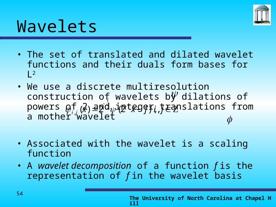
Wavelets

• The set of translated and dilated wavelet functions and their duals form bases for L2

• We use a discrete multiresolution construction of wavelets by dilations of powers of 2 and integer translations from a mother wavelet

• Associated with the wavelet is a scaling function• A wavelet decomposition of a function f is the

representation of f in the wavelet basis

jijxx ii

ji ,),2(2)( 2,


55

Wavelets

• Wavelet coefficients are coefficients of the wavelet decomposition of the form

• Scaling coefficients are those of the form

• Wavelets are usually associated with a pair of a filters, typically a scaling filter H and a wavelet filter G. Once we have a decomposition, reconstruction is performed with dual filters H’ and G’

• Note: terminology can differ depending on source

jiij ff ,,)(

jiij ffs ,,)(


56

Wavelet decomposition

• We decompose a signal by passing it through a each of these filters in a prescribed manner

• Each si is an approximation of our original signal f (the scaling coefficients) at resolution i, and each wi is the wavelet coefficients which can be used as a metric of how the approximation at level i differs from level i-1

fH

G

s1

w1

H

G

s2

w2

H

G

….

….


57

1D Wavelet Example

Input Signal (Using a level 2 coiflet)


58

1D Wavelet Example

H

G

Level 1 Decomposition


59

1D Wavelet Example

H

G



60

1D Wavelet Example


Showing all the wavelet coefficients as well as the level 4 scaling coefficients

You can see that that scaling coefficients (a4) capture the underlying idea of the original signal


61

Wavelet-based Heuristic

• We establish a heuristic based on the rule: Do not cross areas with large higher resolution wavelet coefficients. – For smooth parts of the terrain, the L2 approximation

error decays rapidly towards finer scales– For noisy parts, the higher resolution coefficients are

uniformly large, but the lower resolution coefficients take on the shape of the underlying signal

– Based on the wavelet used, areas of high variation will show up more prominently in the wavelet coefficients


62

Path costs

• Must watch out for “the ravine effect.”– If there is a small region of uniformly high cost

(a ravine, for instance), then certain metrics such as max cost will cause every path to have the same cost

• Instead, use Dsmax(p), for a path p

– Dsmax(p) =list of costs for each node in p in sorted order

– We can define a <= operator for this, and by tracking each part of the path we eliminate the ravine effect


63

Algorithms

• This papers give algorithms for each of the following to solve the terrain planning problem– Terrain preprocessing– Obstacle computation– Path finding– Path refinement


64

Terrain Preprocessing

• Compute a 2D wavelet decomposition on the sampled terrain f, giving a sequence of scaling coefficients ( ) and wavelet coefficients ( ) for each level l– The scaling coefficients give us approximate

terrain surfaces at different levels– Note that in the 2D case, we have 3 sets of

wavelet coefficients, , , and for horizontal, vertical, and diagonal respectively

ljslj

Hlj V

lj Dlj


65

One level of Terrain Approximation

s is the approximate surface (scaling coefficients) and w is the errors (wavelet coefficients)


66

Obstacle Computation

• We want to restrict the path on several criteria– Terrain slope

• Can’t go across terrain that is too steep– Contact constraints

• Must have a certain number of contacts with the ground

– Static stability constraints• The robot’s center of gravity must be supported

– Collision avoidance constraints• Parts of the robot can’t intersect the terrain or other

parts of the robot

• Go through the surface and label regions as obstacles or free


67

Terrain Obstacles ExampleSlope obstacles (slopes more than about 22 degrees)


68

Path Finding

• Essentially a Dijkstra’s single source shortest path algorithm. Uses the path cost from earlier

• Correctness comes from fact that Dsmax behaves like non-negative addition with the operator


69

Path Refinement

• Takes path p from initial level l• Expand p into channel P with margin m

– If p is a level l path, a cell with index(u,v) is in P if some cell (i,j) is in p and and

– At the next level l -1, mark cells not in P as obstacles, and update terrain obstacles in P

– Perform the path finding algorithm from before with costs from level l -1• This construction greatly reduces the amount of

data to explore at given level

miu )(mjv )(


70

Results

• Notation: – (a -> b) is the path found starting at

coarse level b and refined to a


71

Results

(4 -> 4) path


72

Results

(3 -> 4) path


73

Results

(2 -> 4) path


74

Conclusions

• Advantages– Relatively quick for large terrains– Smaller errors favors not too much to consider

during refinements– Paths tend to prefer large, smooth sections for

travel

• Disadvantages– Wavelet decomposition can take a long time– Smoothness of surfaces dependent upon

wavelet basis


75

Outline






76

Local Multiresolution Path Planning

Behnke, S. Proceedings of RoboCup 2003 International Symposium.


77

Idea

• Do not try to solve entire problem at once, but only use information immediately available

• Use higher resolutions for the configuration space closer to robot, and lower resolutions for space farther away

• Great for constraints seen in applications like RoboCup

• Similar to the quadtree approach


78

Basic Method

• Once again, A* search for the least cost path to the target

• Assign a cost to grid cells that is dependent upon the distant to each obstacle, let it decrease linearly to zero as we move farther away– Sensors can provide these values

quickly, but the certainty decreases for objects farther away


79

Non-Uniform Resolution

• We construct the grid by placing multiple grids of size MxM concentrically– The inner part, [1/4M,3/4M][1/4M,3/4M],

is left empty at this resolution, and the next finest resolution is placed there, until the highest resolution is reached

– This greatly reduces the number of grid cells when compared to a uniform resolution


80

Grid ExampleUniform resolution grid Multiresolution grid

Multiple resolutions shown side by side


81

Additional Heuristics

• We must assign a heuristic that represents both the grid and path cost– Use the grid cost from before as a base

cost– Set the heuristic to be the Euclidean

distance to the target, weighted by the base cost.


82

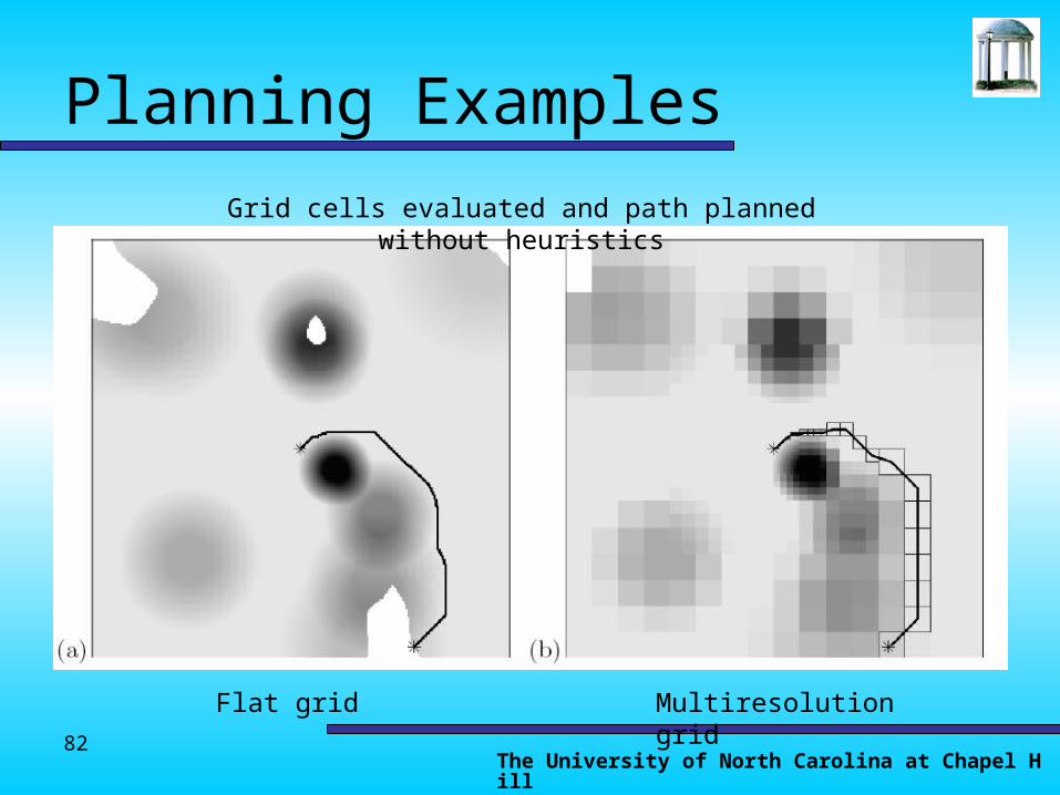
Planning Examples

Flat grid Multiresolution grid

Grid cells evaluated and path planned without heuristics


83

Planning Examples

Flat grid Multiresolution grid

Grid cells evaluated and path planned with heuristics


84

Continuous Path Planning and Execution

• Simulate initial velocity of the robot by placing an obstacle behind it– The larger the obstacle, the larger the

initial velocity

• Re-plan the path based on sensor data– As we move closer to once far away

obstacles, we gain precision about that obstacle and can update the path accordingly


85

Different Initial Conditions

Differing Initial Velocities

Paths made based on different initial values


86

Conclusions

• Much fewer grid cells must be inspected

• The planner runs quickly, allowing for paths to be recomputed in real time– This works because only the part of the

path computed in detail (near the robot) is executed immediately

• The quick run time may allow for a similar algorithm in greater dimensions


87

The University of North Carolina at Chapel Hill 1 Multiresolution Methods in Path Planning Russell...

Documents

Transcript of The University of North Carolina at Chapel Hill 1 Multiresolution Methods in Path Planning Russell...