A Theory for Multiresolution Signal Decomposition: The ...ee225b/sp10/handouts/mallat-good... · A...

Department of Computer & Information Science

Technical Reports (CIS)

University of Pennsylvania Year

A Theory for Multiresolution Signal

Decomposition: The Wavelet

Representation

Stephane G. MallatUniversity of Pennsylvania

University of Pennsylvania Department of Computer and Information Science Techni-cal Report No. MS-CIS-87-22.

This paper is posted at ScholarlyCommons.

http://repository.upenn.edu/cis reports/668

A THEORY FOR MULTlRESOLUTlON SIGNAL DECOMPOSITION: THE WAVELET REPRESENTATION

S. G. Mallat MS-CIS-87-22

GRASP LAB 103

Department Of Computer and Information Science School of Engineering and Applied Science

University of Pennsylvania Philadelphia, PA 191 04-6389

May 1987

Acknowledgements: This work is supported in part NSF-CEWDCR82-19196 A02, NSF-CER MCS-8219196, NSFIDCR-8410771, Air ForcelF49620-85-K-0018, ARMY DAAG-29-84-K-0061, DAA29-84-9-0027 and DARPA NO01 4-85-K-0807 P002.

A THEORY FOR MULTIRESOLUTION SIGNAL DECOMPOSITION :

THE WAVELET REPRESENTATION

STEPHANE G . MALLAT

GRASP lab, Dept of Computer and Information Science University of Pennsylvania Philadelphia, PA 19104-6389

Net address: [email protected]

ABSTRACT

It is now well admitted in the computer vision litemture that a multiresolution decomposition provides a useful image representation for vision algorithms. In this paper we show that the wavelet theory recently developed by the mathematician Y. Meyer enables us to understand and model the concepts of resolution and scale. In computer vision we generally do not want to analyze the images at each resolution level because the information is redundant. After processing the signal at a resolution ro , it is more efficient to analyze only the additional details which are available at a higher resolution rl . We prove that this difference of information can be computed by decomposing the signal on a wavelet orthonormal basis and that it can be efficiently calculated with a pyramid transform. This can also be interpreted as a division of the signal in a set of orientation selective frequency channels. Such a decomposition is particularly well adapted for computer vision applications such as signal coding , texture discrimination , edge detection , matching algorithms and fractal analysis.

1. Introduction In the physical world, the important structures to recognize are of very different sizes. Furthermore,

depending on the distance to the focal plane of a video camera, these elements will appear at different scales on the image. In computer vision we would like to analyze each structure and at the same time process the minimum amount of details necessary to recognize them. One strategy is to process gradually the details with an increasing resolution until the recognition is achieved. For this purpose Witkin [28] has created the scale space representation in which the image appears at several resolutions (or scales) ( r , ) ~ ~ , a (rj < T , + ~ ) . With this representation, after analyzing the image at a given resolution r, , for more details we have to process the image at a higher resolution r,+l . The images at resolutions r, and r;+l give a lot of redundant information. It would be more efficient to process only the additional details available at the resolution r,+l , which we shall call the detail signal at resolution r,+l . For this purpose we will define a new discrete representation called the wavelet representation which provides a coarse approximation of the signal (resolution ro) plus the detail signals at the successive resolutions r; for l l j < N .

The concepts of scale and resolution are interdependent in computer vision. The resolution of an object image gives the minimum size of the object details which will be distinguishable in the image. It is a function of the number of photoreceptors which have measured the light reflected by the object. As there is a finite number of photoreceptors per unit area in the camera focal plane, the resolution will thus depends

This work is supported in part by NSF-CE-82-19196 Am, NSF/DCR-8410771, Air ForceF49620-85-K-0018, ARMY DAAG-29-84-K-0061, and DARPAJONR N0014-85-K-0807.

on the size (or scale) of the projection of the object on this plane. In this paper we will first model the scaling transform which modifies the resolution of the image components. This will then enable us to mathematically define the detail signal at each resolution through a new interpretation of the wavelet theory. Wavelets are particular functions studied by the mathematician Y. Meyer [19] which allow us to build interesting orthonormal bases of L2(Rn) . We will show that the detail signal can be computed by decomposing the original signal on such an orthonormal basis and that it can be efficiently calculated with a pyramid architecture using quadrature mirror filters. The wavelet representation is complete and we will give a similar algorithm for reconstructing the original signal from its decomposition. Like Marr's [18] model the wavelet representation can be interpreted as a decomposition of the original signal into a set of independent orientation selective frequency channels. For two-dimensional signals such as images we will present a separable decomposition which privileges the horizontal and vertical orientations. However the mathematical model enables us to build non-separable representations with as many orientation tunings as desired.

The wavelet representation has many applications in computer vision and signal processing in general. We will describe in particular how it can be used for signal matching , data compression , edge detection , texture discrimination and fractal analysis. Finally, the wavelet representation will be compared with the DOG and Gabor representations currently used in computer vision and having some similar features. We have tried in this paper to give the mathematical insights of the model without justifying in details all the results. The main steps of the theorem proofs are given in the appendices.

2. Scaling transform

We shall hereunder define a scaling transform for one-dimensional signals but the definitions and theorems can be extended to any dimension. We will then study more precisely the two-dimensional case for image processing applications.

2.1. Characterization and modeling

Let T, be the scaling transform which associates to any signal an approximation at a resolution r . Intuitively the resolution r gives the minimum size of the details which can still be found in the approximation, r being defined with respect to a certain distance unit. As described in the introduction, we want to compute the approximation of the original signal at different resolutions and then calculate the detail signals. Koenderink [13] has shown that in order to obtain consecutive detail signals carrying approxima- tively a constant amount of information, the sequence of resolutions should vary exponentially :

(ri)jsz (r > 1) . In order to simplify the computer implementation we will choose r = 2 , but the model can be extended for any r E Q .

We will suppose that our original signal f(x) has a finite energy :

It is well known that there exists an inner product in the vector space L2(R) .

In the computer vision literature certain authors such as Yuille & Poggio [30] and Koenderink [13] have defined several principles forcharacterizing a scaling transform. Hereunder we will describe six such principles with their mathematical interpretation and build a global model characterizing a scaling transform. Having selected the sequence of resolution levels , we will restrict our analysis to the scaling transforms T , which approximate a signal at a resolution 2j .

T , is a linear transformation and if g(x) is the approximation of a signal at the resolution 2i than g(x) is invariant by T , .

T , can thus be interpreted as a projection operator on a particular vector space V, included in L2(R) . Vj is the set of all possible approximated signals at the resolution 2r . We will suppose that the projection

is orthogonal (we can always find an inner product for which this is true).

Causality: The approximation of a signal at resolution 2J+l contains all the necessary informations to build the same signal at a smaller resolution 2J .

Since T p is a projection operator on V, this principle is equivalent to :

A scaling transform does not privilege a priori any particular resolution level. The approximations at different resolutions should thus be derived from one another by using a constant scaling factor. For the sequence of resolutions (2J),,Z this scaling factor is 2 .

+ ' j = Z , g ( x ) e V j <=> g(2x)€Vj+l. (2)

An approximation of a signal at a resolution 2i can be characterized by 2J samples per unit of length.

Because of the previous principle this assertion is valid for all j E Z if it is true for j= 0 . It can thus be written

3 I. isomorphism from Vo onto 12(Z) (3) +a0

where 12(Z)={(ai)iEz / .C, IaiI2 <+) I-

When a function is translated by a length proportional to 2J , its approximation at the resolution 2J is translated by the same length and it will be characterized by the same samples which are translated as well.

Because of (2) it is sufficient to express the above principle for j = 0 . * ~ ( x ) E L2(R) ,-Yk E Z To(f(x))=g(x) <=> To(f (x-k))=g(x-k) (4)

-'k€Z , + ' f ( x ) ~ VO Io(g(x) )=(ai ) iez <=> Io(g(x-k))=(ai-k)i,z. (5)

When the resolution increases towards + the approximated signal converges towards the original signal. Conversely when the resolution decreases to zero, the approximated signal contains less and less information and should ultimately converge towards zero.

Since the approximated signal at a resolution 2J is equal to the orthogonal projection on a space V, , when j increases the space Vi should ultimately cover almost all the initial vector space L2(R) . When j decreases, it should shrink up to the vector space [0) . Property (1) enables us to write this :

j=+- J- ,y Vj is dense in L2(R) and n V, = {O) . I=-- j-

We will call any set of vector spaces ,€ , which verifies the properties (1) to (6) a multiresolution vector space sequence.

From these six principles, we have shown that a scaling transform at a resolution 2J is an orthonor- ma1 projection on a space V, of a multiresolution vector space sequence. In order to compute this orthonormal projection for any signal f(x) , we need to find an orthonormal basis of V, . The following theorem shows that such an orthonormal basis can be computed from a unique function which totally characterizes the multiresolution vector space sequence.

Let V, , be a multiresolution space sequence, then there exists a unique function $(x) called a '"OrernC 1

scaling function such that for any j E Z if @ (x) = 64(2Jx ) then

[$' (X - 2-Jn) ] , is an orthonormal basis of Vj .

Appendix 1 gives the intermediate steps of the proof. We can therefore build an orthonormal basis of any Vj by scaling the function $(x) with a coefficient 2J and translating the resulting function on a grid whose interval is proportional to ZJ . The orthogonal projection on Vj can now be computed by decomposing the signal f(x) on this orthonormal basis.

Let Pv, be the orthogonal projection operator on the vector space V, and let $A (x) = $' (x -Tin) ,

The approximation of the signal f(x) at the resolution 2J is thus characterized by the set of samples :

[ < f .$i>]..,.

As an example we will compute these coefficients for a function f(x) which is constant on a large interval. f(x) = c for x E [2-jn - N ,2-J n + MI with N , M >> ZJ and f(x) = 0 outside this interval.

We can show (appendix 2 (45)) that

For such a function, to have coefficients of same value at all resolutions we need to multiply them by 6 . For any signal f(x) , the set of samples

will be called a discrete approximation of f(x) at the resolution 2J . Since computers can only process discrete signals we will concentrate on these discrete approximations, which completely characterize the continuous approximations. Since

Sj is thus also equal to the convolution of f(x) with W (-x) , sampled at the rate 2J .

s,= [ ~ ( f ( x ) x ~ ( - x ) ) ( 2 - ~ n ) ] (9)

As predicted by the fourth principle, we are now able to characterize the approximation of a signal at a resolution 2J with a discrete signal of 2J samples per length unit.

Fig. 1 shows an exponentially decreasing scaling function. Its Fourier transform has the shape of a low-pass filter, hence equation (8) can be interpreted as a low-pass filtering of the signal. Indeed, we remove all the details smaller than 2J which correspond to the higher frequencies of the signal. We are now going to study a practical procedure to compute the discrete approximations at different resolutions.

2.2. Implementation of a scaling transform

In computer vision as often in signal processing we can only process discrete signals. The measuring device low-passes the input continuous signal and the digitizer provides a uniform sampling at the output. The distance unit will be taken equal to the sampling interval. We can thus consider that these samples give a discrete approximation of the original signal at the resolution 1 : SO.

scanng vuncnon scaring tunctlon touner 1 ransform

[ . . I , . . I . . . . I -5 0 5 -10 0 10

Absclssa Omega

Fig. 1. Example of scaling function with its Fourier transform. It decreases exponentially in the spatial

domain and like in the frequency domain. 3

The causality principle shows that from So we can compute a11 the S, for j < 0 . We shall now prove that this can be performed with a simple recursive algorithm.

For +(x) a scaling function, [ ~ + l ( x ) ] ,=, is an orthonormal basis of V,+l so

+j(x) E Vj c Vj+l can be decomposed in this basis:

thus, < +A , +i+l> = < +ol , +pPh > (1 1)

so* writing the inner product of f(x) with the functions of both sides of equation (9) and multiplying by 42/+l , we have

Let H be a discrete filter with impulse response

and H be the symmetrical filter with impulse response k(n ) = h (-n ) ,

Equation (13) shows that S, can be computed by convolving S,+l with H and by keeping every other sample of the output. All the S, for j < 0 can thus be computed from So by repeating this process for all j < 0 . This is called a pyramid transform. In practice the measuring device only gives a finite number N of samples. We can then easily show that each discrete signal S, (j < 0) will have 2 /N samples. Fig. 2 shows the discrete approximated signal S, of a continuous signal f(x) , for j = 0 , -1 , -2 , -3 . We have approximated the impulse response of the filter H shown in Fig. 3 by taking h(n) = 0 for Inl > 8 . The continuous approximated signals T u ( f ) have been calculated with equation (7) . When the resolution decreases the smaller details of f(x) gradually disappear.

Let us insert equations (1 1) and (12) in (10) . For j = - 1 and n = 0 we have :

Let $(w) and H(o) be respectively the Fourier transform of $(x) and the discrete Fourier transform of h(n) . The Fourier transform of equation (14) can be written

This equation gives a simple relation between the filter H and the corresponding scaling function $ ( x ) . Based on this equation, the following theorem gives a complete characterization of the filter H and shows that given such a filter it is possible to build $(x) . This will enable us to numerically compute some scaling functions. In computer vision we often need to analyze the signal locally both in the spatial and frequency domains. For this purpose, we will look for scaling functions which are well localized in both

1 domains. In particular we will suppose that @(x) = 0 (7) in order to simplify the statement of the X

theorem .

Theorem 2 Let $ ( x ) be a scaling function and H a dlscrete filter with impulse response

h (n) = & <$fl ,$a > and discrete Fourier transform H(o) . H is a low pass filter with the following properties :

(a) H (o) is 2n periodic , differentiable and I H (0) I = 1 . (b) I ~ ( o ) l ~ + IH(wn)I2= 1

Conversely let H be a discrete filter with Fourier transform H(w) satisfying (a) , (b) and such that (c) I H (o) I f 0 for o E [O , n/2]

then, $(a) = fl H (2-P o ) P =

(16)

is the Fourier transform of a scaling function, and

Appendix 2 gives some indications to prove this theorem. The filters which verify the property (b) are called quadrature filters. We can find an extensive description of such filters and numerical methods to synthesize them in the signal processing literature [5,20,25]. Given a quadrature filter H which verifies (a) , (b) and (c) we can then compute the corresponding scaling function with equation (16) . It is possible to choose the filter H so that the scaling function $(x) will be well localized in both the frequency and spatial domains. In appendix 3 we give a class of symmetrical scaling functions which are

1 exponentially decreasing and whose Fourier transforms decrease like l;- for n E N . The scaling func- o tion shown in Fig. 1 is one of them. We can also find quadrature filters H having a Finite Impulse Response (h(n) = 0 for Inl > no) [%I. This leads to non symmetrical scaling functions which have a compact support [3] in the spatial domain. Fig. 3 shows the H filter of the scaling function given in Fig. 1.

3. The wavelet representation

3.1. Detail signal modeling

We do not want to process the signal at each resolution because the information is redundant. It is more efficient to successively process the details which can be found at the resolution 2i+l but not at the resolution 2J . The approximations of the signal at the resolution 2i+l and 3 are given respectively by the orthogonal projection of the signal on Vitl and V, . By applying the projection theorem we can easily show that the detail signal at the resolution 2J+l are given by the orthogonal projection of the original signal on a vector space 0, such that:

0, is orthogonal to Vj

oj s v, = v,+l . For computing this orthogonal projection for any signal f(x) we need to find an orthonormal basis of 0, .

~ont~nuous Approx at nesolutlon 1 ~ ~ s c r e t e Approx at nesolutlon 1

~ontlnuous ~ p p r o x at neso~utlon I I Z ulscrete ApprOX at nesolutlon I I Z

I _ . _ . I . . . . I _ . .

0 100 200 Abscissa

-

.-- . - C

A. -. - r s -

: 75 * -- - .- .- * - .A ' -+:3- :. ?. .

--- -.- - - 2

- < r : I . I . . . . I . . .

1

F U

0.5 C t I

: O :

v p -0.5 U 6

-1

t l . . . . I . I .

0 100 200 Absclssa

0 100 200 0 100 200 Absclssa Absclssa

- 1

S a

- m 0.5 P

0 O -

v a I

- u -0.5 0 s

- -1 I . . . . I . . . . I _ . .

-1 I . . . . I . , . . I . . .

0 100 200 Absclssa

r ; . . . . I . . . . I . . . 0 100 200

Absclssa

~ont~nuous ApprOX at neso~ut~on IILI u~screte ApprOX at nesolut~on ,/a

I . . . . . . . . I . . .

0 100 200 Absclssa

v a 1 -0.5 U 8 S 1, l ; , , , , , ~ , - ; ; ; , . , : , ~ , , m - ~ ~ ; , ; . -

-1

0 50 100 150 200 250 Absclssa

Fig. 2. The left and right images are respectively [he graphs of S, and T,(f ) for j = 0 , -1 , -2 , -3 (resolution 1 ,112 ,114 , 118). When the resolution decreases smaller details gradually disappear.

n unpulse nesponse

0.6 r

n ulscrete tourler I ransrorm

I

C . . ! . . . . I I . . . .

-2 0 2 Omega

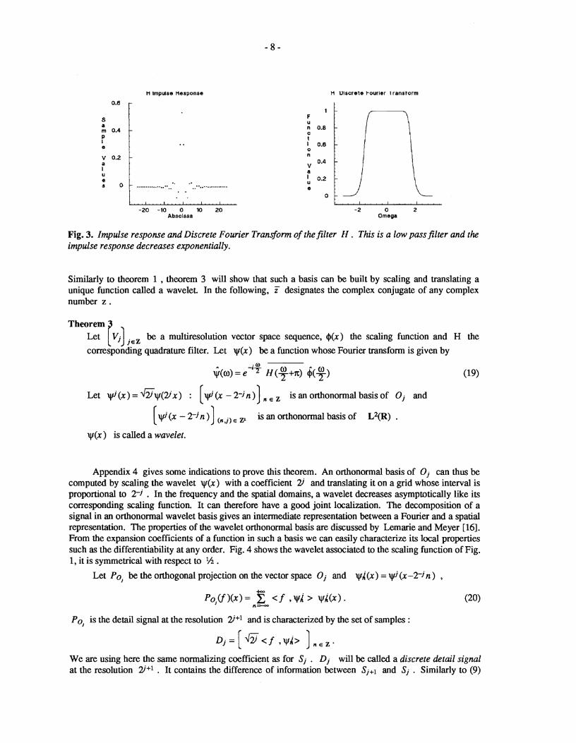
Fig. 3. Impulse response and Discrete Fourier Transform of the filter H . This is a low pass filter and the impulse response decreases exponentially.

Similarly to theorem 1 , theorem 3 will show that such a basis can be built by scaling and translating a unique function called a wavelet. In the following, Z designates the complex conjugate of any complex number z .

j s z be a mulLiresolution vector space sequence, 4(x) the scaling function and H the

corresponding quadrature filter. Let ~ ( x ) be a function whose Fourier transform is given by

Let $ ( ~ ) = 6 ~ ( 2 J x ) : [ ~ I J ( X - 2 - j n ) ] n e , isanorthonormalbasisof 0, and

[ ~ ( x - Z J ~ ) ] b j , e z2 is an orthonormal basis of L2(R) .

~ ( x ) is called a wavelet.

Appendix 4 gives some indications to prove this theorem. An orthonormal basis of Oj can thus be computed by scaling the wavelet ~ ( x ) with a coefficient 2J and translating it on a grid whose interval is proportional to 2-J . In the frequency and the spatial domains, a wavelet decreases asymptotically like its corresponding scaling function. It can therefore have a good joint localization. The decomposition of a signal in an orthonormal wavelet basis gives an intermediate representation between a Fourier and a spatial representation. The properties of the wavelet orthonormal basis are discussed by Lemarie and Meyer [16]. From the expansion coefficients of a function in such a basis we can easily characterize its local properties such as the differentiability at any order. Fig. 4 shows the wavelet associated to the scaling function of Fig. 1, it is symmetrical with respect to ?h .

Let PO, be the orthogonal projection on the vector space 0, and ~ i ( x ) = (x-2-Jn ) ,

Po, is the detail signal at the resolution 2J+l and is characterized by the set of samples :

We are using here the same normalizing coefficient as for S, . D, will be called a discrete detail signal at the resolution 2i+l . It contains the difference of information between S,+l and S, . Similarly to (9)

wavelet MOIUIUS or wavelet tourler I ransform

[ . . I . . . . ) . . . I . .

-5 0 5 -10 0 10 Absclssa Omega

Fig. 4. Example of wavelet with the modulus of its Fourier transform. It decreases exponentially in the 1 spatial domain and like in the frequency domain.

we can prove that

~ ( x ) can also be viewed as a band pass filter and equation (19) shows that the detail signal at each resolution correspond to a particular frequency band of the signal.

We can now easily prove by induction that for any J < 0 , the original discrete signal So can be represented by the set of discrete signals

SJ (q)/Sjcl 1 . This is called a wavelet representation. It gives a reference signal at a low resolution SJ and the detail signals at the resolutions 3 for J S j I - 1 . It can be interpreted as a decomposition of the original signal in an orthonormal wavelet basis or as a decomposition of the signal in a set of independent frequency channels like in Marr 's 1181 human vision model. The independence is due to the orthogonality of the wavelet functions. However it is very difficult to have a real understanding of the model in terms of frequency decomposition because the frequency channels overlap and there is some aliasing. We can control this aliasing thanks to the orthogonality of our decomposition functions. This is why the tools of functional analysis give a better understanding of this decomposition. However, we will see that if we neglect this aliasing problem the interpretation in the frequency domain provides an intuition for understanding to the model.

3.2. Implementation of the wavelet representation

We are first going to show in this paragraph that we can compute the wavelet representation with a pyramid transform. As for S, , D, can indeed be easily derived from S,+l . W ~ ( X ) E Oj c Vj+1 , SO it can be expanded in an orthonormal basis of Vj+1

Like for (1 1) , by changing variable in the inner product integral we can prove that :

hence, by taking the inner product of f(x) with the functions of both sides of equation (22) we get :

Let G be the discrete filter with impulse response

and G be the symmetrical filter with impulse response g ( n ) = g (-n ) ,

Equation (25) shows that we can compute D, by convolving S,+l with the filter G and keeping every other sample of the output.

1 : suppress every two sample

: convolve with filter X

Fig. 5. Pyramid architecture for computing the wavelet representation of a one-dimensional signal.

Similarly to (15) , if we insert equations (23) and (24) in (22) , for j= -1 and n = 0 we have

Let G (o) be the discrete Fourier transform of g(n) . The Fourier transform of equation (26) can be written :

From equation (19) of theorem 3 we can then derive that

G (a) = e-io H (wn) and thus g (n ) = (- 1)'-" h (1-n )

G is the mirror filter of H , it is a high-pass filter.

li lrnpulse nesponse MOOUIUS 01 U U I S C r ~ 1 ~ FOUrIer 1 ranstorm

-2 0 2 Omega

Fig. 6. Impulse response and Discrete Fourier Transform of the filter G . This is a high pass filter and the impulse response decreases exponentially.

Fig. 6 shows the mirror filter G of the filter H given in Fig. 3. In signal processing G and H are called [51 quadrature mirrorfilters. Equation (25) can be interpreted as a high-pass filtering of the discrete signal Sj . S,+l is decomposed into S, and D, which respectively keeps the lower and higher frequencies. If the original signal has N samples, D, as well as S, will have 2 - N samples, so the wavelet representation

has the same number of samples as So

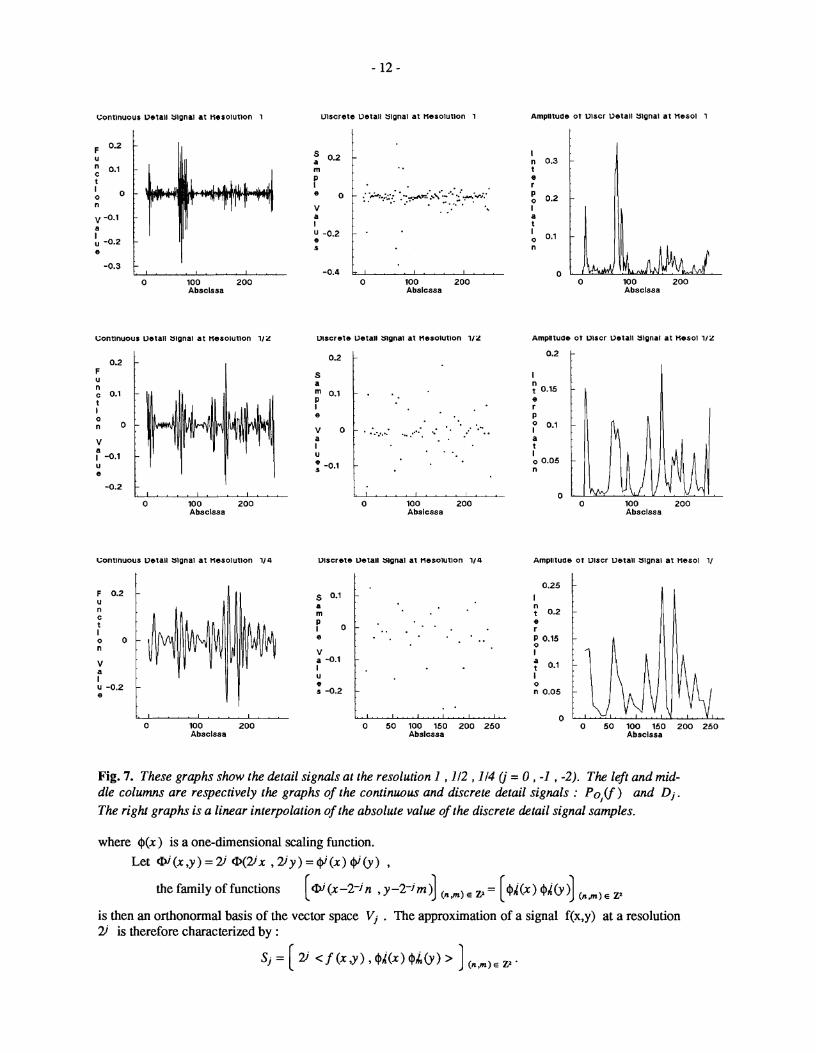
Fig. 7 shows the detail signals of the signal So at the top of Fig. 2. The middle and the left graphs of Fig. 7 are respectively the discrete and continuous detail signals Dj and Po,(f) . We have approximated the filter G shown in Fig. 6 by taking g(n) = 0 for Inl > 8 . Po,(f) can be easily calculated from Dj with equation (19) . On the left column of Fig. 7 we have plotted a-linear interpolation of the absolute value of the detail signal samples. A signal edge contains high frequencies and thus corresponds to the amplitude peaks of the detail signals. Depending on how straight the edge is, the peak will be found at the resolution 1 or 112 . However the highest peak at the resolution 1 is due to the "texture" between the abscissa 60 and 80 and not to an edge. This kind of problem which arises for any edge detector shows that we need a more sophisticated model to separate the edges from the rest of the signal. The differentia- tion between edges and textures depends on the scale of observation. What can be labeled an edge at one scale can be considered as a texture component at a smaller scale. We hence believe that a multiresolution analysis of signals can improve edge detection.

We know that the wavelet representation is complete and are now going to prove that the original discrete signal can onstructed with a pyramid transform. From assertions (17) and (18) we can easily derive that is an orthonormal basis of Vj+l . Therefore, @/+l(x) can be decomposed in this basis

By taking the inner product of each side of equation (29) with the function f(x) and inserting equations (10) and (23) , we have

Introducing (12) and (25) in this expression, we get f

Equation (31) shows that Sj+l can be reconstructed by putting zeros in between each sample of S, and D j , convolve them respectively with the filters H and G , add the two outputs and finally multiply the result by 2 . The original discrete signal So can then be reconstructed by repeating this procedure for J S j < 0 as illustrated by the block diagram in Fig. 8. Fig. 9 shows the reconstruction of the discrete signal So given in Fig. 2 from its wavelet representation (J = -3) . By comparing the two graphs , we can see that the quality of the reconstruction is very good. The smooth as well as the most irregular parts of the signal are well rebuilt. This illustrates the numerical stability of the decomposition and reconstruction processes.

4. Extension to two dimensions The wavelet model can be easily generalized to any dimension n E N' [ll] but we will study in

particular the two-dimensional case for image processing applications. The signal is now a function f (x ,y ) E L2(R2). We define identically a sequence of multiresolution vector spaces and the approximation of a signal f(x,y) at a resolution 3 is still equal to its orthogonal projection on the corresponding vector space V, . In this paper we will only study the particular case of two-dimensional scaling transformations which are built by scaling the signal both along the x and y axis. For computer implementation this will indeed allow us to compute a two-dimensional wavelet representation with separable filters, which reduces the computation complexity. Furthermore in such an approach we privilege the detail signal in the horizontal and vertical directions which are often the predominant directions of the image structures. Such scaling transforms are characterized by scaling functions which can be written

0

-0.3 I . . . . I _ . I . . 0 100 200

Absclssa

-0.2 1

I . , . . I . . . I . . . 0 100 200

Absclssa

0 100 200 Abslcssa

" 0 100 200

Absclssa

u~scre le vetall bwgnal at nesolutlon 112 Ampntuae of v~scr uetall signal at uesol llz

, , ; . . . . l . , . . l . . .

0 100 ZOO Abslcssa

0 100 200 Absclssa

0 100 200 Absclssa

., 0 50 100 150 200 250 0 50 100 150 200 250

Abslcssa Abscissa

Fig. 7. These graphs show the detail signals at the resolution 1 ,112 ,114 fj = 0 , -1 , -2). The left and middle columns are respectively the graphs of the continuous and discrete detail signals : Po,( f ) and D;. The right graphs is a linear interpolation of the absolute value of the discrete detail signal samples.

where @(x ) is a one-dimensional scaling function. Let @(x,y) =2 @ ( a x , 2 y ) = @ ( x ) w(y) ,

the family of functions [a (x-2-jn , y -2-J m )] I, ,, , = [ O ~ ( X ) 9t (y )] (,,,, , , is then an orthonormal basis of the vector space V; . The approximation of a signal f(x,y) at a resolution 2J is therefore characterized by :

If 2 put one zero between each sample : convolve with fllter X : multlply by 2

Fig. 8. Pyramid architecture in one dimension for reconstructing the original signal from its wavelet decomposition.

Fig. 9. The left graph is the discrete reconstruction of the approximated signal at the resolution I . The right graph gives the corresponding continuous signal. The quality of the reconstruction can be appreciat- ed by comparing these graphs with the top graphs of Fig. 2.

neconstr o t L'ontlnuous Approx at nesol 1 neconstr or u~scre te Approx at nosol 1

Similarly to (8) , in two dimensions we normalize the expansion coefficients with 2 because

1 1

F S u a

0.5 m 0.5 C t P I

I 0 :: O v a v I

f -0.5 u -0.5 e

U 0

s

-1 -1

Fig. 10 gives the discrete approximations of an image for j = 0 , -1 , -2 , -3 . Like in the one-dimensional case, the detail signal at the resolution 2r+' is equal to the orthogonal

projection of the signal on a vector space Oi characterized by equations (17) and (18) . The following theorem gives a simple extension of theorem 3 and defines an orthonormal basis of 0, in order to compute the orthogonal projection.

- ? :. . - i

*+-: -- : f

0 - : 5 .

:-y* -. -%

- .- . - ..? - - Y - . . -. -. b- ,- - - 2

- 5 -: I I . I .

0 100 200 0 100 200 A b s c l s s a A b s c l s s a

Fig. 10. Approximations of an image at the resolution 1 ,112 ,114 ,118 (j = 0 , -1 , -2 , -3).

Theorem 4 Let Q(x ,y) = @(x) $ 6 ) be a two-dimensional scaling function and yr(x) the one-dimensional wavelet associated to the one dimensional scaling function @(x) . Then the family of functions

is an orthonormal basis of Oj and

is an orthonormal basis of L2(R2) .

Appendix 5 gives the intermediate steps of the proof. The difference of information between Sj+l and Sj is now given by three detail signal images:

Like in the onedimensional case, we will suppose that the output of the image digitizer is equal to So . For any J c 0 , the discrete image can be thus be completely represented by the -35 + 1 discrete images :

[ SJ ( D j l ) ~ ~ + l 9 ( D ? ) J ~ + I 9 ( ~ j ? J S j + l ] . This is the wavelet representation in two dimensions. SJ is the reference coarse image and the D,! give the detail signal for the different orientations and resolutions. If the original image has N2 pixels the images Sj-l , Dt-1 , D$l , D,& will have each 2-N2 (i c 0) pixels. The total number of pixels in this new representation is equal to the number of pixels of the original image, so we do not increase the volume of data.

Similarly to (9) and (21) , Sj and the signal details D,L can also be written

The expressions (32) , (33) , (34) and (35) show that in two dimensions, S, and the D,! are given by separable filtering of the signal along both the x and y axis. The wavelet decomposition can thus be interpreted as a signal decomposition in a set of independent, spatially oriented frequency channels. We can easily derive from our one-dimensional analysis that this wavelet representation can also be computed with a pyramid transform as shown in Fig. 11. It corresponds to a separable quadrature mirror filter decomposition [29]. We successively filter the rows and the columns of the S, images at each resolution with the filters H and G defined previously.

columns

columns

rows

[ : convolve (rows or columns) with the filter X

: suppress every two columns

: suppress every two rows

Fig. 11. Pyramid architecture for computing the wavelet representation of a two-dimensional signal.

Supposing that o(x) and ~ ( x ) are respectively a perfect low-pass and band-pass filter, Fig. 12(a) shows in the frequency domain how the discrete signal Sj+l is decomposed into S j , D ) ,D; and D? . S, corresponds to the lowest frequencies, D ) gives the vertical high frequencies (horizontal edges) at the resolution 3 + l , 0; the horizontal high frequencies (vertical edges) and D/3 the high frequencies in both directions (comers) . This is well illustrated by the decomposition of a white square on a black back- ground shown in Fig. 13(b). All of the two-dimensional wavelet decompositions shown in this paper have been computed with the one-dimensional filters shown in Fig. 3 and Fig. 5. The arrangement of the D,! images is shown in Fig. 12(b). The black, grey and white pixels respectively correspond to negative, zero and positive coefficients. In Fig. 13(c) we have shown the absolute value of the detail signal samples. The black pixels correspond to zero whereas the white ones have the highest amplitude. As expected, the detail signal samples have high amplitude respectively on the horizontal edges, the vertical edges and the comers of the square. Fig. 14(b) shows the wavelet representation of a natural scene image for J = -3 , and Fig. 14(c) gives the absolute value of the detail signal samples. The arrangement of the images is explained in Fig. 12(b). Like in one dimension, the maximum amplitude of the detail signals samples correspond to edges and rough textures area but it also provides an orientation discrimination.

The image 14(a) was provided by the Qualibrated Imaging Lab at CMU funded by the National Science Foundation.

Fig. 12. (a) Repartition in the frequency domain of the discrete images . (b) Arrangement of the D,! and Sj in the wavelet representation images.

I I n (c)

Fig. 13. (a) Original image. (b) Wavelet representation for J = -2 . (c) Absolute value of the detail signal pixels.

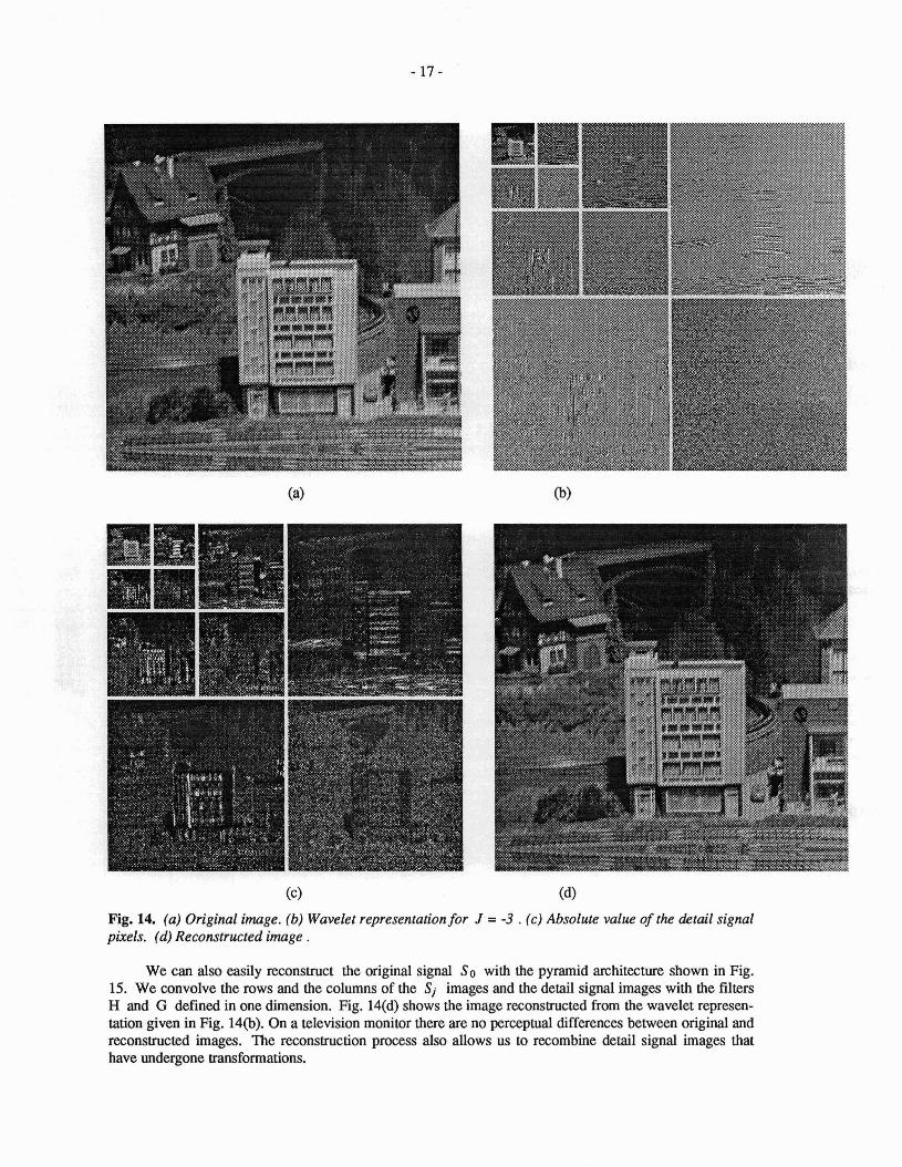
Fig. 14. (a) Original image. (b) Wavelet representation for J = -3 . (c) Absolute value of the &tail signal pixels. (d) Reconstructed image .

We can also easily reconstruct the original signal So with the pyramid architecture shown in Fig. 15. We convolve the rows and the columns of the S, images and the detail signal images with the filters H and G defined in one dimension. Fig. 14(d) shows the image reconstructed from the wavelet representation given in Fig. 14(b). On a television monitor there are no perceptual differences between original and reconstructed images. The reconstruction process also allows us to recombine detail signal images that have undergone transformations.

rows columns

rows columns

: convolve (row or column) with filter X

ITfl : put one row of zeros between each row - : put one column of zeros between each column

: multiply by 4

Fig. 15. Pyramid architecture in two dimensions for reconstructing the original signal from its wavelet decomposition.

5. Applications of the wavelet representation

In a wavelet representation the detail signals reveal some information about edges, oriented textures and gross structures which are not as easily accessible in the original image. The image is decomposed in a set of detail signals which contain the information about all the physical structures which appear specifi- cally at a given resolution. For the separable scaling transform we have considered, the detail signal images give the horizontal, the vertical edges and the "comers" at each resolution. SJ gives locally the DC component of the image. This representation enables us to select a priori the relevant image information for a particular goal. Let us suppose we want to analyze a photograph taken by a satellite whose distance to the earth is known. We can compute at which resolution will appear the patterns we are looking for and therefore select the relevant detail signal images which contain the interesting information. In order to recognize a continent it is clear that we only need a very coarse description of the image which can be found in SJ and the D," (k=1,2,3) for j small. Conversely, to characterize the local vegetation we just have to analyze the D," for j big.

Another important application is signal matching. The goal is to find the position of a given pattern in an image. This kind of problem arises when we try to find some feature correspondence between several images in order to extract the depth or to measure the local motion. We can compute the wavelet representation of both the reference pattern and the image and then correlate the two representations with a coarse-to-fine strategy. First the coarser levels of the representations are put in correspondence and if the matching seems admissible we continue with the higher resolution image details. For most cases, the coarse resolution information is sufficient to eliminate the mismatches so we do not have to process the finer details, which saves computation. The orientation discrimination of our representation has some interesting applications when there is a preferred orientation in the matching problem. If we want to match a pair of stereo images for example, we know that the disparity is horizontal so the matching has to be found on a horizontal line called epipolar line. Such a matching can only be achieved by using the horizontal high frequencies (vertical edges) so we do not have to correlate the D) images.

In order to speed up the algorithms as well as save memory, it is important to reduce as much as possible the amount of data necessary to code the image. The orthogonality of the wavelet functions insures that we do not keep any redundant information, consequently we do not increase the number pixels for representing the same image. In addition, as can be seen on the images 13(b) and 14(b) , the variance of

the detail signal images is much smaller (by two or three orders of magnitude) than the variance of the original image. With standard signal processing techniques, [29], we can thus reduce considerably the number of quantization levels while having the same quantization noise. Humans have different sensitivity to the image noise depending on the frequency band where it occurs. They are most sensitive at middle frequencies and not so sensitive at very low or very high frequencies [15]. The detail signal at each resolution corresponds to a particular frequency band of the image, we can thus adapt the level of the quantization noise to the human sensitivity in the corresponding frequency band [2].

We have seen that the wavelet representation could be used for edge detection. We are now going m describe the potential applications for texture discrimination. In psychophysics Julesz [12] has shown that humans analyze textures by decomposing them with a set -of basic functions called textons. These textons are spatially local, they have a particular spatial orientation and a narrowfrequency tuning. The wavelet representation can also be interpreted as a texton decomposition where each texton is equal to one function of the wavelet orthonormal basis. Indeed, these functions have all the discriminative abilities required by the Julesz theory. It is easy to show that the detail signal at the resolution 9 of a certain texture is equal to the detail signal at the resolution 2+' of the same texture seen from twice the distance. It is thus possible to analyze the texture gradient due to perspecte by comparing the detail signals when the resolution varies. In the decomposition studied in this paper we only have two orientation tunings but we could build a wavelet representation having as many orientation tunings as desired by using non-separable wavelet orthonormal bases [ll]. Fig. 16(a) shows three textures synthesized by J. Beck. The human can not preattentively discriminate the middle from the right texture but can separate the left texture. In this example, the human discrimination is based mainly on the orientation of these textures as their frequency content is very similar. With a first order statistical analysis of the wavelet representation shown in Fig. 16(b), we can also discriminate the left texture but not the two others. It illustrates the ability of our representation to differentiate textures on orientation criteria. This is of course only one aspect of the problem and a more sophisticated statistical analysis is needed for modeling textures [7]. Although several psychophysical stu- dies have shown the importance of a signal decomposition in several frequency channels [9,1], there still is no statistical model to combine the information provided by the different channels. From this point of view, the wavelet mathematical model might be helpful to transpose some tools currently used in functional analysis to characterize the local regularity of functions.

Mandelbrot [17] has shown that some natural texture images can be modeled by fractal noise. A fractal noise F(x) is an ergodic random process which is self-similar

3 H > 0 , +'r E R , F (x) and r H F (rx) are statistically identical.

A realization of F(x) will thus look similar at any scale and for any resolution. Fractals do not provide a general model which can be extended for any kind of textures, however Pentland [24] has shown that for a fractal texture the psychophysical perception of roughness can be quantified with the fractal dimension. Fig. 17(a) shows a realization of a fractal noise which looks like a cloud. Its fractal dimension is 2.5 . Fig. 17(b) gives the absolute value of the detail signal pixels; we can see that the detail signals are similar at the different scales. The S-3 image gives the local DC component of the image which would correspond to the local differences of illuminations for a cloud. We are now going to show that the fractal dimension can easily be computed from the wavelet representation. We will give the proof for a one-dimensional fractal noise but it can be easily extended to G o dimensions. The power spectrum of a fractal noise is given by [I71

The fractal dimension is related to the exponent H by

D = T + l - H

where T is the topological dimension of the space in which x varies (for ima es T = 2). We have seen

output. The power spectrum of the filtered signal is ? in (21) that the detail signals Dj are obtained by filtering the signal with 2J v j ( - x ) and sampling the

Fig. 16. (a) JBeck textures : only the left texture is preattentively discriminable. (6) Absolute value of the wavelet representation for J = -3 : the left texture can be discriminated with a first order statistical analysis of the detail signals.

Pj(tO)=P(tO) l\ir(2-'0)1~ . After sampling at a rate 9 , the power spectrum is given by 1221

Let 07 be the variance of the detail signal Dj ,

By inserting equations (37) and (38) in (39) and using the change of variable a' = 2 0 in this integral we can prove that

07 = 22" 0;+1 . (40) 0 2

For a fractal, the ratio -5 should thus be constant. Equation (40) enables us to compute H and then 0,+1

the hctal dimension D ;nay be computed with equation (36). This proof does not use any specific property of the wavelets and the same result can be derived with other functions such as the Gabor functions [lo]. In two dimensions we can derive an equation similar to (40) for each orientation tuning of the detail signal. For the fractal shown in Fig. 17(a) we have calculated these ratios in each orientation for the first three levels. The maximum error on the fractal dimension derived from each of these ratios was 3% .

We will now briefly compare the wavelet representation with some others which have similar properties and are currently used in computer vision. The Difference Of Gaussians representation is computed by filtering the image with a set of filters equal to the difference of two gaussians of different variance. Such a representation can be interpreted as a decomposition of the signal into a set of non-oriented frequency channels and can also be built with a pyramid architecture [21]. Since the decomposition functions are not orthogonal the DOG representation increases the number of pixels by a factor of 4/3. There is no

Fig. 17. (a) Fractal noise. (b) Wavelet representation for J = -3 . The detail signals are similar for each resolution.

model which enables one to handle easily the redundancy of this representation, so it artificially increases computations. Moreover this representation does not have any orientation discriminability which is incon- venient for some computer vision applications such as texture segmentation.

Recently Daugmann [4] has reintroduced the Gabor representation for decomposing images. The Gabor filters are fixed variance Gaussians modulated by sinusoidal waves of different frequencies. They ate orientation selective and have an optimal joint resolution in the spatial and frequency domains and have orientation tunings. We will briefly summarize some arguments discussed by A.Grosmann [8] explaining some numerical instabilities of this representation. A Gabor decomposition is similar to a Fourier expansion but it is local because of the Gaussian window. For a signal which varies quickly with respect to the size of the window, a Gabor expansion behaves essentially like a discrete Fourier transform. It is well known that the Fourier expansion of irregular signals is very unstable because it adds many high frequency sinusoidal waves, of comparable amplitude and rapidly varying phase. The same problem appears in the Gabor expansions and J.Morlet [8] has shown for example that the Gabor coefficients could not give a robust characterization of seismic signals. In image processing such signals would correspond to the irregular textures. Some researchers [27] are now modifying the variance of the Gaussian window in the Gabor representation but it is not clear whether this new representation is complete or what its properties are.

6. Conclusion In this paper we have described a mathematical model which enables us to understand the concept of

resolution and how it relates to scale. We have seen that it is possible to compute the difference of information between different resolutions and thus define a new complete representation called the wavelet representation. It corresponds to an expansion of the original continuous signal in a wavelet orthonormal basis but can also be interpreted as a decomposition in a set of independent frequency channels with orientation tunings. The wavelet functions can be well localized both in the spatial and frequency domains so that this decomposition gives an intermediate representation between both domains. The representation is not redundant because the wavelet functions are orthogonal; it thus keeps constant the number of pixels to

code the image. The wavelet representation can be efficiently implemented with a pyramid architecture using quadrature mirror filters and the original signal can also be reconstructed with a similar architecture. The numerical stability is well illustrated by the quality of the reconstruction.

The orientation selectivity of this representation is useful for many applications. We have discussed in particular the application of the wavelet representation to signal matching, data compression, edge detection, texture discrimination and fractal analysis. Computer vision applications have been emphasized but this representation can also be helpful for pattern recognition in other domains. Grossmann and Kronland- Martinet [14] are currently working on speech recognition and J.Morlet on seismic signal analysis. The wavelet orthonormal bases are also studied both in pure and applied mathematics and have found some applications in Quantum Mechanics with the work of T. Paul [23] and P. Federbush [6].

Acknowledgments I would to like to thank particularly R. Bajcsy for her advice and guidance throughout this research,

and Y. Meyer for his help with the mathematical aspects of this paper. I am also grateful to J. Vila for his comments.

Appendices

In these appendices we will give the intermediate steps for proving the theorems without going into the mathematical details. Appendix 1 gives the proof of theorem 1 and some of the results are used in appendix 2 to prove theorem 2. Appendix 3 describes a particular class of scaling functions among which the scaling function used in this paper was chosen. Appendix 4 and 5 give the proof of theorem 3 and 4.

Appendix 1

Proof of theorem 1 We will prove theorem 1 for j = 0 but the result can be extended for any j E Z by using equation (2) Following equation (3) and (5) ,

I

1 i f k = O A ~ ( x ) E V o suchthat Io(g)=eo where E O ( ~ ) =

Any function f ( x ) E V o can thus be written

Let g(o) and f ( w ) be the Fourier transform of g(x) and f(x) , +-

f ( o ) = M ( o ) g ( w ) with M ( o ) = x a k e i k a k-

(41)

We are looking for a function @(x) E Vo such that k , z is an orthonormal family. With the Poisson formula we can show that it is equivalent to

From equations (41) and (42) we can thus derive a necessary condition on &a) :

Q(w) = Mo(o) i (o) with Mo(o) = E l ( w 2 k d l [k- 1 -" (43)

The continuity of the isomorphism l o enables us to find two constants C 1 and Cz such that

C J

We can then conclude from (44) that (43) defines a unique function @(x ) where @(x -k ) k , z is orthonormal and complete in Vo . I 1

Appendix 2

Proof of theorem 2 (a) : H (a) is a discrete Fourier transform and is therefore 2n: periodic.

1 1 @ ( x ) = 0 (F) SO < @gl , $2 > = 0 (?) hence H (o) is differentiable.

It is possible to prove that the property (6) of a multiresolution vector space sequence implies that

We have seen in (14) that

thus IH(0)I = 1 . (b) : From equation (42) and (46) we can derive that

IH(o)12+ IH((wn))I2= 1 .

Conversely we are going to show that the equation

Qo) = Q H (2-p o) P=

defines the Fourier transfo of a caling function. We need to prove that: E LYR) and 7 ,(x 9 ae , is an orthonormal basis of a vector space V,

,€, is a multiresolution vector space sequence.

Property (a) is equivalent to : f

Let us define the sequence of functions of L2(R) gp (o) ,>, such that I 1 gP(o )=f i~ (2 -pw) for < 2 x , and &(o)=0 for l w l 2 l x . (49)

converges towards 14(o) 1 almost everywhere. We can easily prove that r

By using the hypothesis (c) of it is then possible (elaborate) to apply the theorem of dominated convergence to the sequence and therefore prove that @(a) verifies (48) .

To prove that [v,] ,€, is a multiresolution vector space sequence we need to show that the assertions (1) to (6) apply. We can derive (46) from the hypothesis (47) . It can then be shown that + u p ) E Z2 , U(X) is a linear combination of the functions [4j(x)] nE, so Vj c V,+l ,

Equations (2) to (5) are not difficult to prove. (6) can be derived (elaborate) from property (45).

Appendix 3

In this appendix we describe a class of symmetrical scaling functions first discovered by P.Lemarie

and G.Battle, which decrease exponentially in the spatial domain and like 1- in the frequency domain. 0"

Let

We can compute the close form of C, (61) by taking the successive derivatives of the formula

A Franklin scaling function of order n is defined by I

It is then possible to show that N x ) = 0 (e"m'x') where a,, is a positive coefficient depending on n. For a Franklin scaling function of order n, the vector space V, is the set of all functions which are n - 2 times continuously differentiable and equal to a polynomial of degree n - 1 on the intervals [2-j k ,2-J (k+l ) ] . Fig. 1 shows a Franklin scaling function of order 4 .

Appendix 4

Proof of theorem 3 . This theorem will also be proved for j = 0 . We are looking for a sequence of functions which would be an orthonormal basis of O0 . We have seen in (26) that

\ i r ( 2 ~ ) = G ( w ) ~ ( o ) . f >

(51)

Similarly to (42) , Lv(x -n )j .. is orthonormal if and only if

thus I G ( o ) I 2 + IG(wrc)I2= 1 . (52) I >

(18) each function of the family ..z must be orthogonal to each function of .. z . With the Poisson formula this +'=

+n E Z C @ ( w 2 n n) v ( w 2 n rc) = 0 n-

which is equivalent to -

H (o) G (w) + H ( w n ) G ( w n ) = 0 . (53)

Conversely we can prove that the relations (51) , (52) and (53) are also sufficient for building a wavelet orthonomal basis of 0 . A solution of (52) and (53) is given by

G ( o ) = e"O H ( w n ) .

From (6) , (17) and (18) one can easily derive that for j # j', 0, is orthogonal to Of and

L2(R) = 8 0, .

Since is an orthonormal basis of 0, , [ y ~ ~ ( x - 2 - ~ n ) ] , j , . is therefore

Appendix 5

Proof of theorem 4

We will prove in this appendix that the family of functions :

[ 0 1 ( x ) y ~ c v ) , ~ l ( ~ ) @ i ( V ) . v l ( x ) v i c v ) ] (,,,).,.

is an orthonormal basis of 0, . Let V,1 and 0: be respectively the vector space generated by [ ~ ( x ) ] , and [ @ i ( x ) ] , .

Let us write 0 the tensor product of vector spaces,

v. ]+I- -v.l ]+I BVbl =(oj' 8vi') a (O; Qvj9

hence Vj+l=(Vf OV;) Q (V) 0 0 ) ) Q ( 0 1 B V j ' ) O ( 0 ; 0 0 1 ) .

v j = v i ' 0vi' thus O,=(V,J 630; ) 0 ( 0 ) r8Vi ' ) Q (Oi' 0 0 1 ) .

We can therefore conclude that the family (54) is an orthonormal basis of 0 , .

References

[l] J. Beck, A. Sutter and R. Ivry, "Spatial frequency channels and perceptual grouping in texture segre- gation," CVGIP, vol. 3, Feb. 1987.

[2] P.J. Burt, A. E. Adelson, "The laplacian pyramid as a compact image code" IEEE Trans. Communi- cations vol. 31, pp 532-540, Apr. 1983.

[3] I. Daubechies, "Orthonormal bases of compactly supported wavelets," Bell lab., 1987.

[4] J. G. Daugmann, "Six formal properties of two dimensional anisotropic visual filters. Structural principles and frequency / orientation selectivity," IEEE Trans. System Man and Cybernetics, vol. 13, Sept. 1983.

[5] D. Esteban and Galand C., "Applications of quadrature mirror filters to split band voice coding scheme," Proc. ICASSP May 1983.

[6] P. Federbush, "Quantum field theory in ninety minutes," Dept. Math. Uni. of Michigan, 1986.

[7] A. Gagalowicz, "Vers un modele de textures," These de docteur d'etat, INRIA, France, May 1983.

[8] P. Goupillaud, A. Grosmann and J. Morlet, "Cycle octave and related transform in seismic signal analysis," vol. 32, pp85-102, 1985186.

[9] N. Graham, "Psychophysics of spatial frequency channels," pp. 215-262, Erlbaum, Hilldasle, N.J., 1981.

[lo] D. Heeger and A. Pentland, "Measurement of fractal dimension using Gabor filters," Tech. Rep. TR 391, SRI A1 center.

[Ill S. Jaffard, P. G. Lemarie, S. Mallat and Y. Meyer, "Multiscale analysis," Centre Math., Ecole Polytechnique, Paris, 1986.

[12] B. Julesz, "Textons, the elements of texture perception and their interaction," Nature vol. 290, Mar. 1981.

[13] J. Koenderink "The structures of images," Bwlogical Cybernetics, Springer Verlag, 1984. [14] R. Kronland-Martinet, J. Morlet and A. Grosmann, "Analysis of sound patterns through wavelet

transform," International Journal on Pattern Analysis and Artifzcial Intelligence, vol. I , Jan. 1987.

[15] J. Kulikowski and A. Gorea, "Complete adaptation to patterned stimuli: A necessary and sufficient condition for Weber's law of contrast," Vision Res., vol. 18, pp. 1223-1227,1978.

[I61 P. G. Lemarie and Y. Meyer, "OndeIettes et bases hilbertiennes," Revista Mathematics Ibero- Americana, vol. 2, 1986.

[17] B. Mandelbrot, The fractal geometry of nature, W . H . Freeman and co., New-York, 1983.

[18] D. Marr, Vision W. H. Freeman and co., 1982.

[I91 Y. Meyer, "Principe d'incertitude, bases hilbertiennes et algebres d' operateurs," Bourbaki seminar, n. 662, 1985-86.

[20] P. Millar and C. Paul, "Recursive quadrature mirror filters; criteria specification and design method," IEEE Trans. ASSP, vol. 33, pp. 413-420, Apr. 1985.

[21] P. Burt, "Fast filter transforms for image processing," CGZP, vol. 16, pp. 20-51,1981.

[22] A. Papoulis, Probability, random variables and stochastic processes, Mc Graw-Hill Book, New- York, 1984.

[23] T. Paul, "Affine coherent states and the radial Schrodinger equation. Radial harmonic oscillator and hydrogen atom," sent for publ.

[24] A. Pentland, "Fractal based description of natural scenes," IEEE Trans. PAMI, vol. 6 , pp. 661-674, 1986.

[25] G. P i n i and V. Zingarelli, "Analytical formula for design of qudrature mirror filters," IEEE Trans. ASSP, vol. 32, pp. 645-648, Jun. 1984.

[26] M. J. Smith and T. P. Barnwell, "Exact reconstruction techniques for tree-structured subband coders," IEEE Trans. ASSP, vol. 34, Jun. 1986.

[27] M. Turner, "Texture discrimination by Gabor functions," Biological Cybernetics, vol. 55, pp. 71-82, 1986.

[28] A. Witkin, "Scale space filtering," Proc. Int. Joint Conf. Articial Intell., 1983.

[29] J. W. Woods and S. D. O'Neil, "Subband coding of images," IEEE Trans. ASSP, vol. 34, Oct. 1986.

[30] A. Yuille and T. Poggio, "Scaling theorems for zero crossings," IEEE Trans. PAMI, vol. 8, Jan. 1986.

A Theory for Multiresolution Signal Decomposition: The ...ee225b/sp10/handouts/mallat-good... · A...

Documents

Transcript of A Theory for Multiresolution Signal Decomposition: The ...ee225b/sp10/handouts/mallat-good... · A...