THE ROLE OF LOCAL AND REGIONAL FACTORS IN THE …
178
University of Missouri, St. Louis University of Missouri, St. Louis IRL @ UMSL IRL @ UMSL Dissertations UMSL Graduate Works 5-8-2007 THE ROLE OF LOCAL AND REGIONAL FACTORS IN THE THE ROLE OF LOCAL AND REGIONAL FACTORS IN THE FORAGING ECOLOGY OF BIRDS ASSOCIATED WITH POLYLEPIS FORAGING ECOLOGY OF BIRDS ASSOCIATED WITH POLYLEPIS WOODLANDS WOODLANDS Grace Patricia Servat-Valenzuela University of Missouri-St. Louis, [email protected] Follow this and additional works at: https://irl.umsl.edu/dissertation Part of the Biology Commons Recommended Citation Recommended Citation Servat-Valenzuela, Grace Patricia, "THE ROLE OF LOCAL AND REGIONAL FACTORS IN THE FORAGING ECOLOGY OF BIRDS ASSOCIATED WITH POLYLEPIS WOODLANDS" (2007). Dissertations. 588. https://irl.umsl.edu/dissertation/588 This Dissertation is brought to you for free and open access by the UMSL Graduate Works at IRL @ UMSL. It has been accepted for inclusion in Dissertations by an authorized administrator of IRL @ UMSL. For more information, please contact [email protected].
Transcript of THE ROLE OF LOCAL AND REGIONAL FACTORS IN THE …

University of Missouri, St. Louis University of Missouri, St. Louis
IRL @ UMSL IRL @ UMSL
Dissertations UMSL Graduate Works
5-8-2007
THE ROLE OF LOCAL AND REGIONAL FACTORS IN THE THE ROLE OF LOCAL AND REGIONAL FACTORS IN THE
FORAGING ECOLOGY OF BIRDS ASSOCIATED WITH POLYLEPIS FORAGING ECOLOGY OF BIRDS ASSOCIATED WITH POLYLEPIS
WOODLANDS WOODLANDS
Grace Patricia Servat-Valenzuela University of Missouri-St. Louis, [email protected]
Follow this and additional works at: https://irl.umsl.edu/dissertation
Part of the Biology Commons
Recommended Citation Recommended Citation Servat-Valenzuela, Grace Patricia, "THE ROLE OF LOCAL AND REGIONAL FACTORS IN THE FORAGING ECOLOGY OF BIRDS ASSOCIATED WITH POLYLEPIS WOODLANDS" (2007). Dissertations. 588. https://irl.umsl.edu/dissertation/588
This Dissertation is brought to you for free and open access by the UMSL Graduate Works at IRL @ UMSL. It has been accepted for inclusion in Dissertations by an authorized administrator of IRL @ UMSL. For more information, please contact [email protected].

THE ROLE OF LOCAL AND REGIONAL FACTORS IN THE FORAGING ECOLOGY OF BIRDS ASSOCIATED WITH POLYLEPIS WOODLANDS
THE ROLE OF LOCAL AND REGIONAL FACTORS IN THE FORAGING ECOLOGY OF BIRDS ASSOCIATED WITH POLYLEPIS WOODLANDS
Grace P. Servat
Master of Science, University of Missouri at St. Louis, St. Louis-August 1995
A dissertation submitted to the Graduate School of the University of Missouri at St. Louis
in partial fulfillment of the requirements for the Doctoral degree in Arts and Sciences
July 25, 2006 Advisory Committee Bette Loiselle, Ph.D. Advisor John G. Blake, Ph.D. Robert Ricklefs, Ph.D. George Taylor, Ph.D. External Committee Member
ii

ABSTRACT
THE ROLE OF LOCAL AND REGIONAL FACTORS IN THE FORAGING
ECOLOGY OF BIRDS ASSOCIATED WITH POLYLEPIS WOODLANDS
Understanding the extent to which patterns of functional structure and organization
are repeated in space and time and the level or scale at which different factors (local and
regional) operate to explain community patterns are of central importance in studies of
community ecology.
In this dissertation, I studied the extent of spatial variation in foraging ecology of
birds in the Polylepis community, a unique vegetation association of the Andes, in regard to
variation in local (e.g.,, vegetation structure, floristic composition, food resource availability)
and regional factors (e.g.,, biogeography). I used a pluralistic approach with detailed studies
of foraging ecology of nine insectivorous bird species (and the assemblage they conform)
across twelve disjunct Polylepis woodlands embedded in three biogeographic regions of the
Peruvian Andes. I focused the study on foraging ecology (i.e., maneuvers and microhabitat
use) because the ways in which individuals forage influenced their performance. Natural
selection should favor those strategies that maximize fitness, or some proxy of fitness, e.g.,,
rate of resource acquisition, production of offspring.
I examined the extent of spatial variation in foraging ecology at species and
assemblage levels. At species level, I assessed intraspecific variation using two foraging niche
components: breadth and plasticity, both of which provide complementary information at
different spatial scales and levels of organization (e.g., species, populations). Niche breadth
measures if the species is a specialist (i.e., uses a relatively limited fraction of the range of
available resources) or generalist (i.e., uses a relatively large fraction of available resources)
relative to other community members or species in a clade. Niche plasticity evaluates how
restricted or plastic are intraspecific regularities in the niche. Thus, a species is restricted if
its niche is consistent across populations, and plastic when niche regularities across
populations break down. Results indicate that foraging niches of bird species varied in a
continuum from specialist-restricted (i.e., consistently narrow foraging niche) to generalist-
plastic (i.e., highly variable and broad niche). With the exception of one specialist-restricted
iii

species (Oreomanes fraseri), foraging ecology of bird species seemed to be influenced mostly
by fluctuations in food resources, floristic composition, and vegetation structure. In
particular, variation in food resources was a predictor of foraging ecology in seven of the
nine bird species studied. Lack of variation in foraging of specialist-restricted species,
despite fluctuations in local factors, may be a consequence of past events in the evolutionary
history of the species that set a limit to the range of possible responses within a population,
constraining the foraging niche.
At the insectivorous assemblage level, I assessed variation in structure using the
conventional guild approach (e.g., guild classification, number of guilds) with the underlying
assumption that species with similar ecological attributes act or respond to environmental
variation in similar ways. I focused on two factors that may influence assemblage structure:
food resources (i.e., arthropod abundance in microhabitats where birds forage) and the
potential effect of biological interactions (i.e., competition). The relative importance of food
resources was assessed by relating site similarities in food resource abundance and site
similarities in richness and abundance of birds within guilds. The potential role of
competition was assessed using null models to determine if patterns of niche overlap among
species in the assemblages were consistent with competition theory. Results indicate that
niche overlap patterns in the assemblage may respond to competitive interactions (i.e.,
assemblage niche overlap was significantly higher than expected by chance). However, food
resources seemed to be of relative less importance in structuring bird assemblages in the
Polylepis community. Guild identities were largely consistent among Polylepis woodlands, with
bark foragers, foliage foragers, and aerial foragers present at most sites. However, the
number and identity of species associated with each guild was not necessarily consistent due
to regional differences in species richness and intrapopulation variation in foraging ecology.
Studies that describe the extent of spatial variation in the structure of communities and the
factors in which the community is embedded are insightful, yet scarce. The present study
acknowledges the complexity of communities as a dynamic collection of species integrated
to varying degrees by ecological and historical factors.
iv

ACKNOWLEDGMENTS
Foremost, I would like to thank T. Erwin, my family and my advisor B. Loiselle for
their support along this long journey. I thank B. Loiselle and the members of my
committee: J. Blake, R. Ricklefs, and G. Taylor for providing scientific advice and
constructive criticism to this study, as well as, thoughtfully reviewing the manuscript. I also
want to thank M. Kessler and all the Blake-Loiselle students in special J. Goerck, L. M.
Renjifo, D. Cadena, L. Lohmann, and J. Perez-Eman for their reviews on the proposal
and/or early versions of the manuscripts, and P. Feria for her support and help with GIS-
based figures. In the field, I benefited from the help of M. Servat, T. Erwin, W. Mendoza, J.
Ochoa, W. Palomino, and many enthusiastic students at Universidad Nacional San Antonio
Abad del Cusco and Universidad Nacional de San Agustin de Arequipa. Funds for this
study were obtained from the International Center for Tropical Ecology at the University of
Missouri-St. Louis (UMSL), the Department of Biology at UMSL, the Carnes Award from
the American Ornithological Union, the St. Louis Rainforests Advocates, and the National
Science Foundation (Award No. 9724719).
v

to Terry
vi

TABLE OF CONTENTS
LOCAL AND REGIONAL PATTERNS OF FLORISTIC COMPOSITION AND VEGETATION STRUCTURE OF POLYLEPIS WOODLANDS IN THE PERUVIAN ANDES......................................................................................................1
METHODS.................................................................................................................... 5 Regional settings ............................................................................................................................5 Local settings.................................................................................................................................6 General study design......................................................................................................................7 Floristic composition and vegetation structure .................................................................................7 Local factors..................................................................................................................................9 Regional factors .......................................................................................................................... 10 Geographic distance .................................................................................................................... 10 Data analysis............................................................................................................................. 11
RESULTS......................................................................................................................14 Floristic composition patterns...................................................................................................... 14 Vegetation structure patterns ...................................................................................................... 16
DISCUSSION ...............................................................................................................17 Floristic composition ................................................................................................................... 17 Vegetation structure ................................................................................................................... 20
REFERENCES ............................................................................................................22
INTRASPECIFIC VARIATION IN THE FORAGING NICHE OF BIRDS ASSOCIATED WITH POLYLEPIS WOODLANDS: THE INFLUENCE OF LOCAL AND REGIONAL FACTORS ......................................................................56
METHODS...................................................................................................................61 Study system............................................................................................................................... 61 Regional settings ......................................................................................................................... 62 Local settings.............................................................................................................................. 63 General study design................................................................................................................... 64 Study birds................................................................................................................................. 64 Variation in local factors............................................................................................................ 66 Data analysis............................................................................................................................. 69 Variation in ecological factors..................................................................................................... 72
vii

RESULTS......................................................................................................................75 Proportional use of foraging categories ......................................................................................... 75 Foraging niche breadth: specialist or generalist?........................................................................... 77 Foraging niche plasticity: restricted or plastic? ............................................................................. 77 Variation in ecological factors..................................................................................................... 78 Local and regional factors and foraging of insectivorous birds ...................................................... 79
DISCUSSION ...............................................................................................................80 Ecological and evolutionary implications of different foraging strategies ........................................ 83
REFERENCES ............................................................................................................86
BIRD ASSEMBLAGE STRUCTURE IN THE POLYLEPIS COMMUNITY..... 125
METHODS................................................................................................................. 129 The study system ...................................................................................................................... 129 The bird assemblage ................................................................................................................. 130 Assemblage structure ................................................................................................................ 132 The potential role of food resource abundance and competition ................................................... 133
RESULTS.................................................................................................................... 134 Assemblage structure ................................................................................................................ 134 Diversity and abundance of insectivorous birds.......................................................................... 136 The relative importance of food resources and competitive interactions in assemblage structure .... 136
DISCUSSION ............................................................................................................. 137 The role of food resource abundance in bird assemblage structure ............................................... 138
REFERENCES .......................................................................................................... 140
viii
LIST OF FIGURES Figure 1.1. Map of the Peruvian Andes showing study regions, Polylepis R. & P. woodlands,
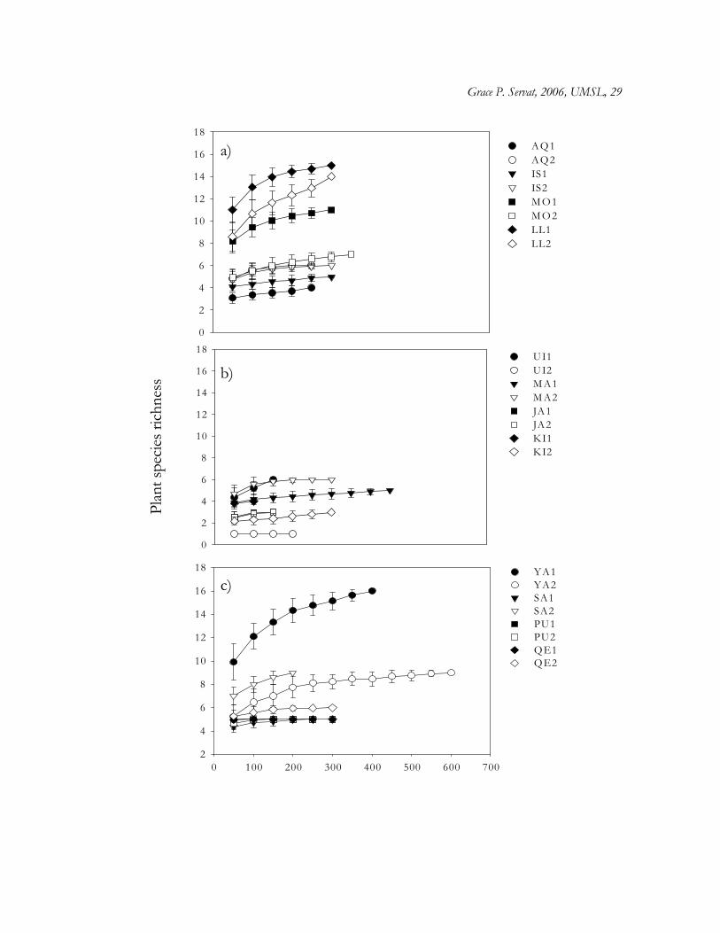
and climate stations mentioned in text. ....................................................................................... 26 Figure 1.2. Plant species richness as a function of species abundance across Polylepis
woodlands plots based on rarefaction analyses.......................................................................... 28 Figure 1.3. Pair-site similarities (Sorensen’s coefficients) in floristic composition of Polylepis
woodlands and regions. .................................................................................................................. 30 Figure 1.4. Arrangement of plots along the first and second axes obtained from Bray Curtis
ordination of floristic composition (presence/absence of 53 plant species) across 24 plots.............................................................................................................................................................. 32
Figure 1.5. Arrangement of plots along the first and second axes obtained from Bray Curtis ordination of 12 vegetation structure variables across 24 plots. ............................................. 34
Figure 1.6. Relative contribution of local and regional factors on floristic composition and vegetation structure of Polylepis woodlands. ................................................................................ 36
Figure 2.1. Schematic diagrams of population niche breadth (A) and plasticity (B). ............ 97 Figure 2.2. Map of the Peruvian Andes......................................................................................... 99 Figure 2.3. Proportional use of foraging categories by arboreal-insectivore birds associated
with Polylepis woodlands. ............................................................................................................... 101 Figure 2.4. Levin’s mean niche breadth (+ SD) for each population of insectivorous bird
species associated with Polylepis woodlands. Low or high values of nic .............................. 103 Figure 2.5. Foraging niche plasticity of insectivorous bird species. ....................................... 105 Figure 3.1. Arrangement of individuals along the first and second axes from Bray Curtis
ordination (based on 25 foraging categories used by birds) of each Polylepis forest. ......... 149 Figure 3.2. Bird species richness (mean + SD) in assemblages, as a function of sample size
compared by rarefaction curves .................................................................................................. 151 Figure 3.3. Bird abundance among guilds in Polylepis woodlands........................................... 153 Figure 3.4. Abundance of bird species and total arthropod abundance (= food resources)
in associated microhabitats........................................................................................................... 155
ix

LIST OF TABLES Table 1.1. Polylepis species present at each woodland and region and local factors measured
at each plot. ....................................................................................................................................... 38 Table 1.2. Mean, variance, and 95 % confidence intervals of plant species richness obtained
by rarefaction .................................................................................................................................... 40 Table 1.3. Multivariate hierarchical ANOVA results for plant species and individuals
number............................................................................................................................................... 42 Table 1.4. Results of Mantel tests.................................................................................................... 44 Table 1.5. Factor loadings for vegetation structure variables along axis 1 and 2. .................. 46 Table 1.6. Multivariate hierarchical ANOVA results for 11 vegetation structure variables. 48 Table 2.1. Polylepis woodlands in the Andes of Peru selected for the present study and dates
of data collection during the two years of study. ..................................................................... 107 Table 2.2. Insectivorous species associated with Polylepis woodlands. ................................... 109 Table 2.3. Inter and intraspecific variation in niche breadth of arboreal-insectivore birds
across forests nested within three regions................................................................................. 111 Table 2.4. Foraging strategies of insectivorous birds. Data in the table includes foraging
niche breadth (Levin’s index) and plasticity results for each bird species........................... 113 Table 2.5. Food resources abundance (arthropods/microhabitat). Hierarchical MANOVA
results for arthropod abundance................................................................................................. 115 Table 2.6. Floristic composition across Polylepis woodlands. ................................................... 117 Table 2.7. Multivariate hierarchical ANOVA results for horizontal vegetation structure
variables. .......................................................................................................................................... 119 Table 2.8. Hierarchical MANOVA results for vertical vegetation structure variables. ...... 121 Table 2.9. Mantel tests using 999 permutations and the program Permute (Casgrain 1998).
........................................................................................................................................................... 123 Table 3.1. Species number in avian assemblages of insectivore forest-interior birds
associated with Polylepis woodlands............................................................................................. 157 Table 3.2. Foraging guilds .............................................................................................................. 159 Table 3.3. Observed and simulated niche overlap values based on foraging categories used
by species in avian assemblages................................................................................................... 161
x

APPENDICES Appendix 1.1. Plant families and species present in Polylepis woodlands in the study area. . 51 Appendix 3.1. Scores (high and low) of foraging categories (in bold) along the first and
second axes of Bray Curtis ordination for each Polylepis woodland...................................... 162
xi

INSECTIVOROUS BIRD SPECIES ASSOCIATED WITH POLYLEPIS WOODLANDS IN THE ANDES OF PERU
xii

Grace P. Servat, 2006, UMSL, 1
CHAPTER ONE
LOCAL AND REGIONAL PATTERNS OF FLORISTIC COMPOSITION AND VEGETATION STRUCTURE OF POLYLEPIS WOODLANDS IN THE
PERUVIAN ANDES
The relative contribution of local, regional and historical processes in structuring
biological communities continues to be a debated issue in community ecology (Latham and
Ricklefs 1993, Ricklefs and Schluter 1993, Francis and Currie 1998, Ricklefs and Latham
1999, Kelt 1999). Local contemporary processes have often been invoked to be of prime
importance in structuring extant communities and, therefore, community attributes are
expected to be strongly correlated with particular local physical and biotic features (Connell
1978, Huston 1979, Keddy 1989, Palmer 1991, Zobel 1992, Aarssen 1992, Tilman and
Pacala 1993). In recent years, conceptual models of community structure have broadened,
and patterns and processes on regional (i.e., biogeography) and historical (i.e., history of
taxa) levels have also been considered to structure ecological communities (Ricklefs 1987,
Cornell and Lawton 1992, Ricklefs and Schluter 1993, Schluter and Ricklefs 1993, Losos
1994, Caley and Schluter 1997, Karlson and Cornell 1998, Losos et al. 1998).
Studies on several taxa support the hypothesis that contemporary communities are
the result of the complex role of the local and regional environment and the evolutionary
and historical relationships of the taxa involved (e.g., Darwin’s finches, Grant 1986;
Caribbean Anolis lizards, Losos 1994, Losos et al. 1998; stream fishes, Angermeier and
Winston 1998; desert rodents, Kelt 1999; plants in calcareous grasslands, Pärtel and Zobel
1999). Consequently, understanding present structure and organization of communities

Grace P. Servat, 2006, UMSL, 2
require multiple analytical approaches that incorporate the local, regional, and historical
factors, as well as chance events in which the community is embedded (Vuilleumier and
Simberloff 1980, Ricklefs 1987, Ricklefs and Schluter 1993, Angermeier and Winston 1998).
Yet, generalizations about the relative importance of particular processes in explaining
community structure and organization depend to a great extent on the ability to delimit the
community itself, and on an adequate knowledge of the patterns of variation of community-
level attributes in space and time.
The high Andes of South America provide an ideal setting to examine the patterns
of spatial variation in fundamental attributes of plant community structure such as floristic
composition and vegetation structure. The diverse topography of Andean mountains results
in a complex mosaic of areas that vary in microclimate, soils, aspect, exposure, and wind
conditions (Walter and Medina 1969, Smith A. 1972, 1977, Smith B. 1988, Sarmiento 1986,
Smith and Young 1987, Young 1992, Fjeldså and Kessler 1996, Young and León 1999), as
well as frequency and intensity of natural (i.e., landslides, Gentry 1982, 1992) and
anthropogenic disturbances (Ellenberg 1958a, 1958b, Laegaard 1992, Hensen 1993, Kessler
1995, Fjeldså and Kessler 1996). This complex set of local conditions creates opportunities
for specialization and adaptation, and has likely led to the heterogeneous distribution of
plants across the Andes (Young 1992, Young and León 1999). However, despite
considerable local variation may occur in Andean systems, patterns of species distribution
across regions may be more regular as a result of shared environmental history. For
instance, the Andes are composed of several independent structural units separated by low
valleys that represent important barriers for dispersal of high elevation elements (Simpson
1975). The movements of plants into high mountain habitats and their subsequent

Grace P. Servat, 2006, UMSL, 3
speciation likely proceeded differently in each section of the Andes. Therefore, the
phytogeographical history of the Andean flora includes shifting climatic zones, vicariant
events, dispersal of montane species, and spread of taxa from other continental floras
(Chardon 1938, Vuilleumier 1971, Simpson 1975, 1983, Ruthsatz 1977, Cleef 1981, Simpson
and Todzia 1990, Kessler 1995, Taylor 1995).
Throughout the high Andes of Peru (ca. 3500-4800 m), forests dominated by the
arborescent genus Polylepis R. & P. (Rosaceae) formed a distinctive and clearly defined
community of exceptional interest in ecology and biogeography. In this community,
woodlands dominated by one and sometimes two or three sympatric Polylepis species
(characterized by gnarled shape with thick and rough, densely laminated bark) occur as small
islands in gorges, on slopes, and along cliff edges. The microclimate, productivity, and
species composition of the woodlands contrast sharply with surrounding grassland habitats
(Weberbauer 1945, Troll 1959, Koepcke H. 1961, Simpson 1979, Vuilleumier 1984, Smith
D. 1988, Kessler 1995, Fjeldså and Kessler 1996). Contemporary patterns of distribution of
Polylepis woodlands have been attributed to microclimatic and physiological requirements of
the plants (Weberbauer 1945, Troll 1959, 1968, Koepcke H. 1961, Walter and Medina 1969,
Simpson 1979, Vuilleumier 1984, Rauh 1988). Alternatively, it has been suggested that these
woodlands are relicts of a habitat that was more widespread during the late Pleistocene (i.e.,
10,000-20,000 years ago) and has become fragmented due to anthropogenic disturbances
(Ellenberg 1958a, 1958b, Beck and Garcia 1991, Fjeldså 1992a, Hensen 1993, Kessler 1995).
The scattered distribution of Polylepis woodlands throughout the Andes provides a
set of discrete and relatively simple systems in terms of plant species composition, when

Grace P. Servat, 2006, UMSL, 4
compared to more species-rich forests at lower elevation, thus facilitating studies on floristic
composition and vegetation structure.
To date, few studies have looked at patterns of spatial variation in floristic
composition and vegetation structure within a local and regional context (Gentry 1982,
1992, 1995, Hensen 1993, Dillon et al. 1995, Sklenar and Jorgensen 1999). Therefore, little is
known about the relative importance that particular local and regional processes play in
structuring Andean communities. Describing patterns of floristic composition and
vegetation structure in contemporary Polylepis woodlands is of considerable importance to
determine the potential mechanisms that likely generate and maintain the structure of the
plant assemblage in this community. Local contemporary patterns of floristic composition
and vegetation structure in Polylepis woodlands might stem from local conditions that favor
the presence of some species in some sites more than in others. Consistent patterns in the
relationship of local floristic composition or vegetation structure to site conditions would
support the hypothesis that local processes are the major determinants of plant assemblage
organization. Conversely, local patterns of floristic composition and vegetation structure
may also stem from regional factors such as large-scale environmental conditions or
physical/biotic barriers to dispersal, in addition to the history of the taxa that make up the
assemblage. Similar patterns of floristic composition and vegetation structure in Polylepis
woodlands within, but not among regions would provide support for a major role for
regional and/or historical processes in determining plant assemblage organization.
The present study is aimed toward documenting the degree of spatial variation in
floristic composition and vegetation structure of plant assemblages across a series of Polylepis
woodlands located in three regions of the Peruvian Andes. The main objectives are: (a) to

Grace P. Servat, 2006, UMSL, 5
describe how Polylepis woodlands vary in floristic composition and vegetation structure
across sites and regions, (b) to determine the scale (local and/or regional) that best explains
patterns of floristic composition and vegetation structure, and (c) to develop hypotheses
regarding the potential causal mechanisms (processes) that influence patterns of floristic
composition and vegetation structure in Polylepis woodlands and the scale at which they
operate.
METHODS
Regional settings
The Andes are differentiated longitudinally into a series of parallel mountain systems
divided along their length into distinct tectonic segments recognizable by surface and
structural features, volcanism, geophysical evidence, and boundaries (Jenks 1956, Petersen
1958, Ham and Herrera 1963, James 1971, Simpson 1975, Smith D. 1988). Three different
regions of the Peruvian Andes were selected for the present study: the Cordilleras Blanca,
Occidental, and Vilcanota. The Marañon River separates the western Cordillera Occidental,
and the eastern Cordillera Oriental (James 1971, Smith 1988) between the Huancabamba
and Abancay deflections (Fig. 1). Each of these mountain systems is composed of a series
of segments. The northern portion of C. Occidental (Ancash Department) is C. Blanca.
Towards the south, (Lima Department) there is a separate segment, hereafter called C.
Occidental (Fig. 1). C. Oriental is also composed of separate segments, including Cordillera
Vilcanota, one of the three study regions (Fig. 1). Despite geological differences, all these
mountain systems reached their present altitude in the Pleistocene or late Tertiary.

Grace P. Servat, 2006, UMSL, 6
The regions selected for this study are recognized to differ biogeographically
(Koepcke H. 1961, Koepcke M. 1961, Simpson 1975, Berry 1982, Lamas 1982, Smith D.
1988, Fjeldså 1992a, 1992b, 1993). In addition, C. Blanca and C. Vilcanota have been
hypothesized to be glacial Pleistocene refuges for a number of taxa (Fjeldså and Kessler
1996) and areas of ecoclimatic stability that have promoted speciation processes (Fjeldså et
al. 1999).
The climate in tropical mountains is characterized by small annual variation in mean
temperature, large variation of daily temperature, and a seasonal pattern of cloudiness and
precipitation (Johnson 1976, Sarmiento 1986). The monthly and annual precipitation and
humidity are quite variable from site to site due to topography (Kessler 1995) but in general,
a dry season characterized by low precipitation and humidity occurs from late April to early
November and a wet season from late November to early April, when moisture is carried
from the Amazon basin by tropical easterlies and clouds form locally by heating of slopes
(Johnson 1976, Smith D. 1988). Climatic data from high mountain areas are scarce and
fragmentary information on temperature, precipitation, and humidity is available only from
stations located in valleys (Smith, D. 1988, Arce 1992, Galiano 1995) (Fig. 1).
Local settings
Within each region, I selected four Polylepis woodlands > 50 ha in size and above
3500 m elevation. At these elevations, distinct woodlands dominated by Polylepis species and
separated by Puna grasslands are a prominent feature of the landscape (Lamas 1982, Kessler
1995). Sites within the same region were selected based on similarities in moisture
conditions and tree architecture of dominant Polylepis species (Table 1). The 12 woodland

Grace P. Servat, 2006, UMSL, 7
sites selected for the present study were: 1) C. Blanca: Aquilpo and Ishinca (dominated by P.
weberbauerii), Morococha and Llanganuco (P. sericea); 2) C. Occidental: Maticuna and Japani
(P. incana), Yaui and Quichas (P. weberbauerii); and, 3) C. Vilcanota: Yanacocha, Sacsamonte,
Pumahuanca, Quenuamonte (P. racemosa) (Fig. 1).
General study design
I studied floristic composition and vegetation structure using a hierarchical sampling
design with four independent woodlands within each of three regions (Cordillera Blanca, C.
Occidental, and C. Vilcanota) (Total woodlands = 12). In each woodland, two sets of four
transects (100 m length and placed 50 m apart from each other) were established in the
forest interior (hereafter referred as plots), separated by at least 500 m (Total plots = 24).
Each plot was located in a homogeneous place regarding aspect and degree of slope. Data
on floristic composition and vegetation structure were taken in eight randomly placed 20 x 5
m belts embedded within the four main transects on each plot (covering a total of 0.08 ha).
Data were combined across the eight 20 x 5 m belts; the experimental unit was each plot.
Floristic composition and vegetation structure
Data on floristic composition and vegetation structure were taken across Polylepis
woodlands from May to December 1997, months that correspond to the dry season and
beginning of the rainy season. Since Polylepis species and most vegetation are evergreen,
changes in season are not expected to have a great impact in the present study.
Floristic composition.- To compare floristic composition across study plots and
woodlands I identified all trees (>10 cm dbh) and shrubs (<10 cm dbh and > 50 cm height)

Grace P. Servat, 2006, UMSL, 8
found in belt transects. The presence (“1”) or absence (“0”) of each plant species was then
included in a plot by plant species matrix for analyses. I built a “floristic composition
distance matrix” to obtain a measure of resemblance between plot pairs using Sorensen’s
similarity coefficient. I used species accumulation curves to examine whether the number of
plant species reached an asymptote. Voucher specimens for all woody plant species were
collected and deposited at the Vargas Herbarium at Universidad Nacional de San Antonio
Abad in Cusco, and the Weberbauer Herbarium at Universidad Nacional Mayor de San
Marcos in Lima.
Vegetation structure.- Aspects of vegetation structure were derived based on
measurements of all woody plants (> 50 cm height). The following structural variables were
calculated to obtain a single measure for each plot per site:
a. Tree size class and mean tree height (HEIGHT).- I measured dbh and height for each
tree in belt transects. I assigned trees to one of three size categories: > 10-20 cm dbh
(DBH1), > 20-30 cm dbh (DBH2), and > 30 cm dbh (DBH3). Height was measured for
each tree encountered using a telemetric graduated pole (12 m, Hastings Telescoping
Measuring Rod); mean tree height was then calculated at the plot level. For analyses, I
combined measures of all trees regardless of species identity.
b. Total basal area (TBA).- I used basal area as a measure of tree species coverage.
TBA was calculated by converting measures of diameter at breast height (dbh) of all trees to
circular area. Tree basal area was then summed across transects to obtain TBA per plot (800
m2).
c. Tree density (TD) and shrub density (SD).- I counted the number of trees (> 10 cm
dbh) within each of the eight 20 x 5 m belts, summed values across all belts within a plot

Grace P. Servat, 2006, UMSL, 9
and divided the total by the area of the plot (800 m2) to get density estimates. I estimated
density of shrubs (< 10cm dbh and > 50 cm height) in a similar manner.
d. Foliage height density (FHDEN) and foliage height diversity (FHD).- Every 20 m along
each of the four 100 m transects within a plot (total n = 24 points per plot), I took
measurements of foliage height density along "vertical" transects with a telemetric graduated
pole. The number of times vegetation “intersected” the pole in a radius of 25 cm was
recorded at the following intervals: 0-2 m (FHDEN1), > 2-6 m (FHDEN2), and > 6-10 m
(FHDEN3). Vegetation contacts were summed within each interval across points and then
divided by total contacts across all heights to obtain a proportion of foliage density
occurring within different heights. The proportion of the vegetation in each interval was
used to calculate foliage height diversity values using the Shannon-Wiener Index
(MacArthur and Horn 1969, James and Shugart 1970).
I built a “vegetation structure distance matrix” to obtain a measure of resemblance
between plot pairs using Sorensen’s dissimilarity coefficient.
Local factors
Many local factors have been suggested to account for contemporary patterns of
distribution of Polylepis woodlands, including features related to topography, edaphic
conditions and microclimate (Simpson 1979, Smith D. 1988, Kessler 1995). Microclimatic
data for Polylepis woodlands, however, and for most Andean forests, is lacking. For the
present study, local conditions were based on a qualitative assessment of each plot. I
obtained data on two topographic features: degree and aspect of slope; and one edaphic
feature: soil texture (Table 1).

Grace P. Servat, 2006, UMSL, 10
Topography.- The aspect and degree of slope influence the amount of solar radiation
received, hence the temperature and moisture regimes (Smith D. 1988). I measured aspect
and degree of slope with a compass and categorized aspect (1=SW, 2=W, 3=N, 4=S, 5=E,
6=NE) and degree of slope (1=50-60o, 2=30-45o, and 3=10-20o) at each plot.
Edaphic conditions.- High Andean soils have variable texture, and the distribution of
plant species may respond to soils with different levels of stone coverage, since previous
studies have shown that stones provide protection mainly due to an increase in soil
temperature (Smith D. 1988). Soil texture was categorized by the percent cover of stones on
the ground; categories included: 1=>50% coverage, 2=>10-50%, and 3=<10%.
Data obtained from local factors were used to construct a “local distance matrix”
using Sorensen’s dissimilarity values between plot pairs.
Regional factors
The study relies on the integration of floristic composition and vegetation structure
patterns nested within three distinct biogeographic regions. I built a “regional distance
matrix” by examining each plot pair and scoring “0” if plots belong to same region and “1”
if they differed.
Geographic distance
I included a measure of geographical distance to understand overall trends of
floristic composition and vegetation structure. I used a map of the Peruvian Andes and
measured the linear distance between the 276 possible pair plots, with the aid of Geographic
Information Systems (ESRI 1992-1997) to build a “geographic distance matrix”.

Grace P. Servat, 2006, UMSL, 11
Data analysis
I analyzed data on floristic composition and vegetation structure of Polylepis
woodlands using univariate and multivariate statistics. I used a combination of hierarchical
Analysis of Variance (ANOVA), Bray Curtis ordination techniques, and Mantel tests to
assess the relative importance of the local and regional factors in explaining patterns of
floristic composition and vegetation structure.
Rarefaction curves.- I used rarefaction analyses (Hurlbert 1971, Simberloff 1972,
Gotelli and Graves 1996) to build species accumulation curves using the EcoSim Program,
Version 5.53 (Gotelli and Entsminger 2000). The program draws a designated random
sample of individuals from a given species abundance distribution to estimate species
richness in regard to sampling effects. Simulations were repeated 1000 times to provide
mean, variance and 95% confidence intervals of species richness at each forest plot based
on different abundance levels to facilitate comparisons among woodland sites and regions.
Analysis of variance models.- To examine if patterns of vegetation structure vary in
woodlands nested within region or across regions, I used a General Linear Model (GLM)
(SPSS 1999) to do hierarchical Multivariate Analysis of Variance (MANOVA) that included
11 vegetation structure variables (TBA, TD, SD, FHDEN1, FHDEN2, FHDEN3, FHD,
HEIGHT, DBH1, DBH2, and DBH3). I used the same analysis of variance model to
examine floristic composition, including total plant species number and total number of
individuals as variables. Normality of each variable was tested using Wilk-Shapiro tests and
variables were logarithmically transformed when necessary. Plots within woodlands were
used as replicates in the design and the null hypothesis was that vegetation structure
variables did not differ across woodlands or regions. More specifically, a significant among

Grace P. Servat, 2006, UMSL, 12
group (F2,9) component will indicate the relative importance of regional factors (i.e., large-
scale environmental conditions, physical/biotic barriers to dispersal, and history of the taxa)
in explaining floristic composition and vegetation structure patterns. If "among forests
within regions" component (F9,12) is found to be significant, then this will indicate the
relative importance of local factors (i.e., aspect and exposure of slope, soil texture) in
shaping floristic composition and vegetation structure. If both terms were found to be
significant then both local and regional processes could be implicated as important
predictors of vegetation structure patterns in Polylepis woodlands. Results of hierarchical
MANOVA were followed by Tukey tests to identify which woodlands and regions were
significantly different from each other.
Bray Curtis ordination.- I analyzed patterns of similarity in floristic composition among
forest plots independently from patterns of similarity in vegetation structure variables using
Bray Curtis ordination (PC-ORD Version 4, McCune and Mefford 1999). I used Sorensen’s
percent dissimilarity as a measure of distance between plots. This index is commonly used
with ecological data because it retains sensitivity in heterogeneous data sets and gives less
weight to outliers (McCune and Mefford 1999). I used the variance regression method for
end point selection and Euclidean distance for axis projection geometry (Beals 1984, Greig-
Smith 1983, McCune and Mefford 1999). The 11 vegetation structure variables (columns)
across 24 study plots (rows) were relativized by column totals to give equal importance to all
variables. The variables for the floristic composition matrix were the presence or absence of
each plant species (columns) across the 24 study plots (rows).
Mantel tests.- I used Mantel tests, a regression approach that compares the
relationship between distance matrices (Mantel 1967, Burgman 1987, Sokal and Rohlf 1995),

Grace P. Servat, 2006, UMSL, 13
to estimate the relative effect of local and regional processes among woodlands or regions in
terms of floristic composition and vegetation structure. Analyses were run using the
program Permute version 3.4, release alpha 5 (Casgrain 1998), a special version of Mantel test
which allows for several predictor variables to be tested over one response variable and
generates partial regression coefficients and the associated permutation probability for each
predictor variable.
Floristic composition and vegetation structure were the response variables and were
represented by distance matrices generated using Sorensen’s percent dissimilarities. Two
separate models were tested, the floristic composition model included three predictor
variables: 1) region (built by examining each plot pair and scoring “0” if plots belong to
same region, and “1” if they differed), 2) geographic distance (built using the actual distance
(in km) between the 276 plot pair combinations); and 3) local variables (a dissimilarity
matrix based on measurements at each plot). The vegetation structure model included: 1)
region, 2) geographic distance, 3) floristic composition (since plant composition may
influence physiognomy), and 4) local conditions, as predictor variables. I selected the
variable(s) that most contributed to explaining variation in structure or composition
dissimilarity matrices using stepwise regression followed by a backward elimination
procedure; 999 permutations of the original matrix were performed to determine the
significance probability of the observed relationship between predictor and response
variables data matrices.

Grace P. Servat, 2006, UMSL, 14
RESULTS
Floristic composition patterns
The forest interior of Polylepis woodlands contained a total of 56 plant species
distributed among 34 genera and 21 families. Asteraceae was by far the most speciose family
(22 species), and within Asteraceae, the most speciose genera were Baccharis (6 species) and
Gynoxys (6 species) (Appendix 1.1). At least 28 genera were represented by only one species.
From the total list of plant species, 30% (17 species) are restricted to high elevations above
3000 m and 23% (13 species) are considered endemic to the Peruvian Andes (Brako and
Zarucchi 1993) (Appendix 1.1).
Plant species sampling in most plots approached an asymptote as revealed by
accumulation curves (Fig. 1.2). Accumulation curves also illustrate the great variation in
plant species richness across sites and regions. When number of individuals is controlled
for, plant species richness differs significantly across Polylepis woodlands and regions (Table
1.2). Basically, more species were found in Llanganuco (average 12 plant species/100
individuals), and one plot in Morococha (average 8 species /100 individuals) (Cordillera
Blanca), and Yanacocha (average 12 species/100 individuals) (C. Vilcanota) than in other
woodland sites (Fig. 1.2, Table 1.2). In addition, hierarchical MANOVA of total number of
species and individuals at each plot revealed significant differences across Polylepis
woodlands (Table 1.3), as well as among regions, with C. Occidental contributing to the
difference in species and individuals number (Table 1.3).
Sorensen’s percent dissimilarity values between woodlands (plots within woodlands
combined) ranged from 0 - 0.52 (0 indicates no similarity, 1 equal or high similarity) (Fig. 1.

Grace P. Servat, 2006, UMSL, 15
3). Results emphasized that forests within the same region tended to be similar in floristic
composition yet regions differed floristically. Similarity values were low even within same
region not only due to differences in plant species composition but also, in most cases, to
differences in species richness in woodlands within the same region. For example, in C.
Occidental, Quichas and Yaui were sites with low species richness that did not share any
species (including Polylepis) with Japani, resulting in low similarity values between these sites
(Fig. 1.3).
Bray Curtis ordination of a presence/absence matrix of 53 plant species across 24
plots revealed similarities in floristic composition within regions (Fig. 1.4). The first three
ordination axes explained 59% of the variance. Axis 1 (29% variation) separated plots in C.
Vilcanota from plots in C. Blanca and C. Occidental (Fig. 1.4). Axis 2 (15%) separated
Ishinca plots from Maticuna (Fig. 1.4), and axis 3 (15%) separated Morococha and
Llanganuco plots from Yaui and Quichas plots. Different species of Baccharis, Berberis,
Gynoxys, and Polylepis had high factor loadings in the two first axes of the ordination, and
therefore contributed to regional separation.
Region and geographic distance explained a large proportion of the variance in
floristic composition as revealed by Mantel test (Table 1.4). A significant positive association
between floristic composition and geographic distance indicates that Polylepis woodland plots
closer together share more species than plots further apart, and that plots within regions are
more similar than plots among regions (Table 1.4). Local factors accounted for only 8% of
the variance in floristic composition (Table 1.4).

Grace P. Servat, 2006, UMSL, 16
Vegetation structure patterns
In general, woodlands dominated by Polylepis racemosa, P. weberbauerii and P. sericea
were more similar structurally than woodlands of P. incana. However, in most cases, plots
from different woodlands showed greater similarity than did plots within the same
woodland (e.g., Morococha, Quenuamonte, and Pumahuanca, Fig. 1.5), suggesting some
degree of local heterogeneity.
Results of the ordination revealed that axis 1 (51%) largely separated Polylepis plots
located in the three regions of study from a set of five plots located in the C. Occidental; the
latter were characterized by low total basal area and greater foliage density below 6 m (Table
1.5, Fig. 1.5). Axis 2 (13%) separated one of the Maticuna plots (T2) from all remaining
ones (Table 1.5, Fig. 1.5). This plot was characterized by greater foliage density below 2 m
(Fig. 1.5). In general, plots in Polylepis woodlands within C. Vilcanota and C. Blanca tended
to have greater basal area, larger trees, and more foliage in the canopy than Japani and
Quichas in C. Occidental.
Vegetation structure in Polylepis woodlands differed significantly both across sites
nested within regions (F9, 12 = 5.83, P < 0.01) and across regions (F2, 12 = 1.86, P = 0.05). All
structural variables differed significantly across sites except tree density (TD) and number of
small trees (> 10 - 20 cm dbh) (Table 1.6). I found significant differences across regions in
all variables except number of small and large trees, foliage density below 2 m, and mean
tree height (Table 1.6).
Patterns of vegetation structure were explained by local variables (exposure and
angle of slope, and soil texture) measured at each plot, as revealed by Mantel test. Floristic
composition and geographic distance also contributed to the variance in patterns of

Grace P. Servat, 2006, UMSL, 17
vegetation structure in Polylepis woodlands (Table 1.4). As geographic distance among plots
increases, plots are more similar in vegetation structure. This result agrees with the Bray
Curtis ordination in which plots of Polylepis woodlands located within C. Blanca and C.
Vilcanota, the two more distant regions in the present study, tend to group together.
DISCUSSION
The role of local and regional factors as significant predictors of floristic
composition and vegetation structure in Polylepis woodlands is summarized in Figure 6.
Regional factors, including history, had important influences on floristic composition but
only contributed indirectly (through their effect on floristic composition) to explain
vegetation structure. Instead, floristic composition and local conditions played a more
important role in determining vegetation structure. In sum, the floristic composition
component of communities, influenced by large-scale environmental and historical
processes, further interacts with local environmental conditions to influence the
physiognomy of the vegetation (cf., Pärtel and Zobel 1999).
Floristic composition
Patterns of floristic composition similarities in Polylepis woodlands were strongly
influenced by regional factors and to a lesser extent by local factors. Floristic composition in
Polylepis woodlands might be linked to present environmental conditions that are shared
within a region, such as precipitation, temperature, and humidity, as has been reported in
many studies in other systems and regions of the world (e.g., Gleason and Cronquist 1964,
Good 1974, Grace 1987, Sykes et al. 1996, Bullock et al. 2000). Indeed, the regions selected

Grace P. Servat, 2006, UMSL, 18
for the present study vary in humidity, and it has been proposed that species richness in
Polylepis woodlands is higher in more humid areas (e.g., C. Blanca and C. Vilcanota) than less
humid ones (e.g., C. Occidental) (Fjeldså 1992a, 1992b, 1993, Fjeldså and Kessler 1996).
However, even though current environmental conditions may explain patterns of plant
species richness, they do not necessarily account for patterns of floristic composition
turnover across regions (Fig. 1.3).
Present distribution of plants inhabiting Polylepis woodlands and similarities within
but not across regions suggests a greater role for environmental history as a determinant of
present day floristic composition. One of the major determinants of floristic composition
changes in recent earth history was the cyclic change in climate and topography during the
Pleistocene (see explanation in terms of global cooling and orbital forcing by Berger et al.
1984, Shackleton et al. 1990, and Hooghiemstra and Ran 1994). Many Cordilleras in Peru
were covered by ice repeatedly over the last 2-3 million years, restricting plant species to
lower elevations on the Andean slopes, and to certain mountain basins that remained ice-
free (Simpson 1975, Simpson and Todzia 1990, Fjeldså and Kessler 1996). The iced-covered
mountain caps may have isolated some refuges with Polylepis woodlands and associated
vegetation from the continuous band of humid shrubbery that is thought to have remained
along the Andes. Isolation during glaciations may have promoted differentiation in certain
genera (e.g.,, Polylepis, Gynoxys), such that distinct species evolved, remaining endemic to their
area of origin (Fjeldså and Kessler 1996). These relict populations that survived periods of
global climatic change likely were the source pool of species for colonization of other areas
as the glaciers receded (Simpson and Todzia 1990, Fjeldså et al. 1999).

Grace P. Servat, 2006, UMSL, 19
In addition, the low floristic composition similarity levels between C. Blanca and C.
Vilcanota observed in the present study could also be attributed to the hypothesis that
Polylepis woodlands were disrupted by tectonics and erosion that created isolation barriers
(e.g., Apurímac Canyon, Fig. 1.1). Such vicariant events preceding Pleistocene glaciations
might have served to isolate relatively non-vagile plants, resulting in pairs of sister taxa on
both sides of each barrier, and thus, influencing community composition across regions. In
contrast, more vagile species are likely to have been less affected because of their ability to
disperse across unsuitable habitats. In such cases, one might expect to see a distance
gradient in community similarities. C. Blanca and C. Occidental were the two regions that
shared relatively more plant species (than did either region with C. Vilcanota). Moreover, a
gradual decrease in species number from north to south suggests a relative larger role for
dispersal between these two regions. Dispersal during interglacial periods and post-glacial
periods could have been an important influence in explaining present floristic composition
patterns (Simpson 1975, Fjeldså and Kessler 1996). The low similarity value between C.
Blanca and C. Vilcanota (0.07 %) could be due to very few species with a wide distribution
throughout the Peruvian Andes that were present before vicariant events, or that dispersed
but were not found in the study area. Further studies are needed to address the history of
taxa, a factor that may contribute with the high percent (53%, Table 1.4) of unexplained
variance found in the present study. Also, tests of biogeographic relationships in which
plant species for which putative phylogenetic reconstructions are available need to be
compared using cladistic analyses (e.g., Brundin 1988, Humphries et al, 1988). In addition,
timing of phylogenetic events (i.e., application of molecular clocks) would also be basic to

Grace P. Servat, 2006, UMSL, 20
discern the relative importance of dispersal and vicariance hypotheses. To date, no parallel
examples for adequate testing exist for plant taxa of the Andes.
The relative influence of local factors in determining present patterns of floristic
composition similarity in Polylepis woodlands was small but significant (b = 0.09*). This
result is not surprising given that few processes could be considered uniquely regional in
scale (Huston 1999). Several studies have addressed fine-scale correlations between different
plant groups and local conditions (Johnston 1992, Clark D. A. et al. 1995, Clark D. B. et al.
1998, Sabatier et al. 1997, Vormisto et al. 2000). Local factors in Japani forest could have
resulted in low species richness and high turnover patterns with respect to other sites in C.
Occidental (Fig. 1.4). In this study, some plant species may be locally adapted to specific soil
texture, topographic positions, and slope angle.
Vegetation structure
Throughout the study area, Polylepis woodlands differed in vegetation structure, and
patterns were influenced by floristic composition and local conditions. The influence of
floristic composition on vegetation structure was expected given the fact that the
combination of plant species present in a community likely contributes to its architecture
and physiognomy. Yet, local conditions, such as aspect, degree of slope and soil texture
affect plant growth, and other structural components of the vegetation. The overall
variation in physiognomy of Polylepis woodlands throughout the study area is likely a
consequence of variation on the morphology and growth forms of Polylepis trees because of
their dominance in the system. Local factors measured in the present study, such as aspect
and degree of slope and soil texture, have been shown to influence local abundance and

Grace P. Servat, 2006, UMSL, 21
growth patterns (i.e., height, branching patterns) of Polylepis and other plant species (Kahn
1987, Smith 1988, Clark D. A. et al. 1995, Clark D. B. et al. 1998, Fjeldså and Kessler 1996).
For example, in C. Blanca Polylepis weberbauerii is found as dense woodlands in which trees
reach 12 m height. In other localities within the same region, however, the same species are
shrub-like reaching only 6 m in height. This variation has been attributed to topographic
position (dense woodlands in south-facing slopes) (Smith 1988) and soil texture (e.g., growth
on boulders) (Smith 1988, Fjeldså and Kessler 1996). Thus, greater similarities in vegetation
structure among Polylepis woodlands located in C. Blanca and C. Vilcanota, the two more
distant regions, can be explained by similarities in local abundance and growth patterns of
Polylepis and other plant species responding to local conditions.
Certainly, other biotic and abiotic factors not measured in this study, such as
microclimatic conditions, local winds (e.g., Smith 1988, Young and Leon 1999), soil
nutrients (e.g., Johnston 1992, Tuomisto et al. 1995), other fine-scale soil conditions (e.g.,
Clark D. A. et al. 1995, Clark D. B. et al. 1998, Sabatier et al. 1997) may be important factors
influencing vegetation structure. Indeed, the high percent of unexplained variance (88%,
Table 4) may be due to these factors. Nonetheless, the results of this study point to the
importance of local factors in explaining patterns of variation in vegetation structure but it
does not separate causal factors from correlative ones.
In summary, the present study provides the first comparative data set on floristic
composition and vegetation structure of Polylepis woodlands on a large spatial scale (ca. 600
km). Little overlap in floristic composition across regions of study suggest a role for regional
factors, including history, while local differences in vegetation structure suggests a role for
floristic composition and local conditions. By using a hierarchical approach, I was able to

Grace P. Servat, 2006, UMSL, 22
better discern local and regional variation in floristic composition and vegetation structure.
This is the first step to generate specific hypotheses regarding the organization of high
Andean communities. The study revealed that identifying the appropriate scale that shapes
patterns of vegetation structure and floristic composition in the Polylepis community requires
knowledge of the regional context in which it is embedded to be able to refine hypotheses
and interpretations regarding community structure and organization. As ecologists continue
to sort out the roles of the many processes involved in community organization, hierarchical
designs that incorporate the local and regional context in which the community is
embedded will become increasingly important in revealing how and where those processes
operate.
REFERENCES
Aarssen, L. W. 1992. Causes and consequences of variation in competitive ability in plant communities. Journal of Vegetation Science 165-174.
Burgman, M. 1987. An analysis of the distribution of plants on granite outcrops in
southern Western Australia using Mantel tests. Vegetatio 79-86. Caley, M. J. and D. S. 1997. The relationship between local and regional diversity. Ecology
78:70-80. Clark, D. A. et al. 1995. Edaphic and human effects on landscape-scale distributions of
tropical rainforests palms. Ecology 76:2581-2594 Clark, D. B. et al. 1998. Edaphic variation and the mesoscale distribution of tree species in
a Neotropical rain forest. Journal of Ecology 86:101-112. Connell, J. H. 1978. Diversity in tropical rain forests and coral reefs. Science 199:1302-
1309. Cornell, H. V. and J. H., Lawton. 1992. Species interactions, local and regional processes,
and limits to the richness of ecological communities: a theoretical perspective. Journal of Animal Ecology 61:1-12.

Grace P. Servat, 2006, UMSL, 23
Ellenberg, H. 1958. Wald oder Steppe? Die naturliche Pflanzendecke der Andes Perus. I
Die Umschau 21:645-648. Farrar, E. and D. C. N. 1976. Timing of late Tertiary deformation in the Andes of Peru.
Geological Society of America Bulletin 87:1247-1250. Fjeldså, J. et al. 1999. Correlation between endemism and local ecoclimatic stability
documented by comparing Andean bird distributions and remotely sensed land surface data. Ecography 22:63-78.
Francis, A. P., and D. J. Currie. 1998. Global patterns of tree species richness in moist
forests: another look. Oikos 81:598-602. Grace, J. B. 1987. Climatic tolerance and the distribution of plants. New Phytology
106:113-130. Ham, C. K., and L. J. H. 1963. Role of the Sub Andean fault system in tectonics of eastern
Peru and Ecuador. American Association of Petroleum Geologists Memories 2:47-61.
Hooghiemstra, H. and T. T. R. 1994. Late Pliocene-Pleistocene high-resolution pollen
sequence of Colombia: an overview of climatic change. Quaternary Int. 21:63-80. Hurlbert, S. H. 1971. The non-concept of species diversity: a critique and alternative
parameters. Ecology 52:577-585. Huston, M. 1979. A general hypothesis of species diversity. American Naturalist 113:81-
101. James, D. E. 1971. Plate tectonic model for the evolution of the Central Andes. Bulletin
of the Geological Society of America 82:3325-3346. James, F. C. and H. H. S. 1970. A quantitative method of habitat description. Audubon
Field Notes 24:727-736. Jenks, W. F. 1956. Handbook of South American Geology. Bulletin of the Geological
Society of America 65: 1-378. Kahn, F. 1987. The distribution of palms as a function of local topography in Amazonian
terra-firme forests. Experientia 43: 251-259. Kelt, D. A. 1999. On the relative importance of history and ecology in structuring
communities of desert animals. Ecography: 123-137.

Grace P. Servat, 2006, UMSL, 24
Koepcke, H. W. 1961. Synoklogische Studien an der Westseite der Peruanishen Anden. Bonner Geographische Abhandlungen 29: 1-320.
Koepcke, M. 1961. Birds of the western slope of the Andes of Peru. American Museum
Novitates: 1-31. Latham, R., and R. Ricklefs. 1993. Global patterns of tree species richness in moist
forests: energy-diversity theory does not account for variation in species richness. Oikos 67: 325-333.
Losos, J. B. 1994. Integrative approaches to evolutionary ecology: Anolis lizards as model
systems. Annual Review of Ecology and Systematics 467-493. Losos, J. B. et al. 1998. Contingency and determinism in replicated adaptive radiations of
island lizards. Science 279: 2115-2118. Palmer, M. W. 1991. Patterns of species richness among North Carolina hardwood
forests: tests of two hypotheses. Journal of Vegetation Science 2: 361-366. Partel, M. Z., M. 1999. Small-scale plant species richness in calcareous grasslands
determined by the species pool, community age and shoot density. Ecography 22: 153-159.
Petersen, U. 1958. Structure and uplift of the Andes of Peru, Bolivia, Chile and adjacent
Argentina. Boletín de la Sociedad Geológica del Perú 33: 57-129. Ricklefs, R. E. 1987. Community diversity: relative roles of local and regional processes.
Science 235: 167-171. Ricklefs, R. E. L., R. E. 1999. Global patterns of tree species richness in moist forests:
distinguishing ecological influences and historical contingency. Oikos 82: 369-373. Sabatier, D. et al. 1997. The influence of soil cover organization on the floristic
composition and structural heterogeneity of a Guianan rain forest. Plant Ecology 131: 81-108.
Simberloff, D. 1972. Properties of the rarefaction diversity measurement. American
Naturalist 106: 414-418. Simpson, B. 1975. Pleistocene changes in the flora of the high tropical Andes.
Paleobiology 1: 273-294. Simpson, B. 1983. An historical phytogeography of the high Andean flora. Revista
Chilena de Historia Natural 56: 109-122.

Grace P. Servat, 2006, UMSL, 25
Simpson, B. T., C. A. Todzia. 1990. Patterns and processes in the development of the High Andean flora. American Journal of Botany 77: 1419-1432.
Sklenar, P. J., P. M. 1999. Distribution patterns of paramo plants in Ecuador. Journal of
Biogeography 26: 681-691. Smith, A. P. 1972. Notes on wind related growth patterns of paramo plants in Venezuela.
Biotropica 4: 10-16. Smith, A. P. 1977. Establishment of seedlings of Polylepis sericea in the paramo zone of the
Venezuelan Andes. Bartonia 45: 11-14. Smith, A. P. Y. T. P. 1987. Tropical Alpine plant ecology. Annual Review of Ecology and
Systematics 18: 137-158. Smith, D. N. 1988. Flora and vegetation of the Huascaran National Park, Ancash, Peru,
with preliminary taxonomic studies for a manual of the flora. Sykes, M. T. et al. 1996. A bioclimatic model for the potential distributions of north
European tree species under present and future climates. Journal of Biogeography 3: 203-233.
Troll, C. 1968. Geo-ecology of the mountainous regions of the tropical Americas.
Colloquium Geographicum 9. Tuomisto, H. et al. 1995. Dissecting Amazonian biodiversity. Science 269: 63-66. Vormisto, J. O. et al. 2000. A comparison of fine-scale distribution patterns of four plant
groups in an Amazonian rainforest. Ecography 23: 349-359. Vuilleumier, B. S. 1971. Pleistocene changes in the fauna and flora of South America.
Science 173: 771-780. Vuilleumier, F. S., D. 1980. Ecology versus history as determinants of patchy and insular
distributions in high Andean birds. Evolutionary Biology 12: 235-379. Walter, H. M., E. 1969. La temperatura del suelo como determinante para la
caracterización de los pisos subalpino y alpino de los Andes de Venezuela. Boletin Venezolano de Ciencias Naturales: 201-210.
Young, K. R. 1992. Biogeography of the montane forest zone of the eastern slopes of
Perú. Memorias del Museo de Historia Natural "Javier Prado" 21: 119-140. Zobel, M. 1992. Plant species coexistence: the role of historical, evolutionary and
ecological factors. Oikos 65: 314-320.

Grace P. Servat, 2006, UMSL, 26
Figure 1.1. Map of the Peruvian Andes showing study regions, Polylepis R. & P. woodlands,
and climate stations mentioned in text. The line indicates the 3,000 m elevation contour. (A)
C. Blanca: 1 = Ishinca (09o22’S, 77o28’W, 4075 m, 200 ha), 2 = Aquilpo (09o21’S, 77o30’W,
3800 m, 200 ha), 3 = Morococha (09o01’S, 77o32’W, 3836 m, 100 ha), 4 = Llanganuco
(09o04’S, 77o38’W, 3850 m, 100 ha). (B) C. Occidental: 1 = Yaui (10o35’S, 76o48’W, 4184 m,
200 ha), 2 = Maticuna (10o39’S, 76o50’W, 3990 m, 200 ha), 3 = Japani (11o41’S, 76o31’W,
4140 m, 300 ha), 4 = Quichas (10o33’S, 76o46’W, 4200 m, 100 ha). (C) C. Vilcanota: 1 =
Yanacocha (13o17’S, 72o03’W, 4012 m, 200 ha), 2 = Sacsamonte (13o13’S, 72o02’W, 3926 m,
100 ha), 3 = Pumahuanca (13o12’S, 72o05’W, 4110 m, 100 ha), 4 = Quenuamonte (13o11’S,
72o13’W, 3812 m, 50 ha). Climatic stations: a = Chinancocha (9o6’S, 77o40’W, 3850m, 8oC,
642mm, and 64%), b = Lampas Alto (10o0’S, 77o20’W; 4030m, 6oC, 737mm, 67%), c =
Carampoma (11o38’S, 76o26’W, 3272m, 12oC, 389mm), d = Urubamba (13 o18’S, 72 o7’W,
2870m, 14oC, 494mm, 66%), e = Calca (13o20’S, 71o57’W, 2859m, 15oC, 437mm).

Grace P. Servat, 2006, UMSL, 27
Grace P. Servat, 2006, UMSL, 27

Grace P. Servat, 2006, UMSL, 28
Figure 1.2. Plant species richness as a function of species abundance across Polylepis
woodlands plots based on rarefaction analyses. (a) Cordillera Blanca, (b) C. Occidental, (c)
C. Vilcanota. Labels in legend represent Polylepis woodlands studied (from North to South),
and numbers (1 and 2) refer to plots (see text for design).
Grace P. Servat, 2006, UMSL, 29
0 100 200 300 400 500 600 7002
4
6
8
10
12
14
16
18 YA1YA2SA1SA2PU1PU2QE1QE2
0
2
4
6
8
10
12
14
16
180
2
4
6
8
10
12
14
16
18
U I1U I2M A 1M A 2JA 1JA 2KI1KI2
AQ1AQ2IS1IS2M O 1M O 2LL1LL2
a)
b)
Plan
t spe
cies r
ichne
ss
c)

Grace P. Servat, 2006, UMSL, 30
Figure 1.3. Pair-site similarities (Sorensen’s coefficients) in floristic composition of Polylepis
woodlands and regions. Higher values for Sorensen’s coefficient imply greater similarity
between two sites or regions.

Grace P. Servat, 2006, UMSL, 31
Cordillera Blanca
Cordillera Occidental
Cordillera Vilcanota
0.20
0.0
0.07
Cordillera Blanca
Cordillera Occidental
Cordillera Vilcanota
0.20
0.0
0.07
Sacsamonte
Quenuamonte
0.35
Pumahuanca
0.36
0.43
0.52
Yanacocha
0.270.25
Sacsamonte
Quenuamonte
0.35
Pumahuanca
0.36
0.43
0.52
Yanacocha
0.270.25
Llanganuco
Morococha
0.41
0.17
0.33
Aquilpo
Ishinca
0.25
0.350.24
Llanganuco
Morococha
0.41
0.17
0.33
Aquilpo
Ishinca
0.25
0.350.24
Yaui
Quichas
0.44
0.18
0.40
Maticuna
Japani
0.0
0.200.0
Yaui
Quichas
0.44
0.18
0.40
Maticuna
Japani
0.0
0.200.0

Grace P. Servat, 2006, UMSL, 32
Figure 1.4. Arrangement of plots along the first and second axes obtained from Bray Curtis
ordination of floristic composition (presence/absence of 53 plant species) across 24 plots.
The asterisk (*) indicates endemic species to the Peruvian Andes. The letters indicate the
forest: A = Aquilpo, I = Ishinca, M = Morococha, L = Llanganuco, U = Yaui, T =
Maticuna, J = Japani, K = Quichas, Y = Yanacocha, S = Sacsamonte, P = Pumahuanca, Q
= Quenuamonte; and numbers (1, 2) indicate the plot.

Grace P. Servat, 2006, UMSL, 33
C. BlancaC. OccidentalC. Vilcanota
DiplostephiumfoliossisimunSpp NI 4
Baccharis salicifoliaLupinus sp.Polylepis incana
Axis 2
(15 %)
Baccharis buxifoliaBerberis carinataGynoxys nitidaPolylepis racemosaRibes brachybrotisSenecio torrehuacensis
Axis 1
(29 %)
Buddleja aff. montanaGynoxys macfrancisciPolylepis weberbauerii
Y1 S1S2 P1P2Y2 Q1
Q2J2
J1
T2 T1
L1
L2
K1 M1 M2 U1
A1 A2K2
U2
I2 I1

Grace P. Servat, 2006, UMSL, 34
Figure 1.5. Arrangement of plots along the first and second axes obtained from Bray Curtis
ordination of 12 vegetation structure variables across 24 plots. The letters indicate the
forest: A = Aquilpo, I = Ishinca, M = Morococha, L = Llanganuco, U = Yaui, T =
Maticuna, J = Japani, K = Quichas, Y = Yanacocha, S = Sacsamonte, P = Pumahuanca, Q
= Quenuamonte; and the numbers (1, 2) indicate the plot.

Grace P. Servat, 2006, UMSL, 35
Axis 1(50.6 %)
Axis 2(13.4 %)
C. BlancaC. OccidentalC. Vilcanota
> Total basal area> Trees 20 - 30 cm DBHFHDEN > 6 m
FHDEN > 2 - 6 m
FHDEN > 0 - 2 m T2
T1
J1K1
J2
P1 K2
M1P2
Q2M2L1
L2 Y1
S2
Q1U2
S1A1A2
I1
U1
I2Y2

Grace P. Servat, 2006, UMSL, 36
Figure 1.6. Relative contribution of local and regional factors on floristic composition and
vegetation structure of Polylepis woodlands. Numbers are partial regression coefficients
obtained from Mantel tests, and asterisks indicate significance levels: * = P < 0.05, ** = P <
0.01, *** = P < 0.001. The contribution of each factor is emphasized by the thickness of the
arrow.

Grace P. Servat, 2006, UMSL, 37
LOCAL FACTORS
Topography Soil texture
REGIONAL FACTORSEnvironment Biogeography
0.36**0.21**
VEGETATION STRUCTURE
0.30***
0.09*
HISTORYOF TAXA
FLORISTIC COMPOSITION

Grace P. Servat, 2006, UMSL, 38
Table 1.1. Polylepis species present at each woodland and region and local factors measured
at each plot. (1) = First notation before slash refers to plot 1 and after slash to plot 2. (2) =
Categories used for stone coverage as a measure of soil texture. 1 = > 50%, 2 = > 10 –
50%, 3 = < 10% (see text).

Grace P. Servat, 2006, UMSL, 39
Region Forest Dominant species Exposure Slope
degree Soil
texture
C. Blanca Aquilpo P. weberbauerii SW/SW 60/60 1/1
Ishinca P. weberbauerii SW/SW 50/50 1/1
Morococha P. sericea W/W 10/45 2/2
Llanganuco P. sericea N/N 10/10 3/3
C. Occidental Yaui P. weberbauerii S/S 60/50 2/2
Maticuna P. incana E/W 30/35 1/1
Japani P. incana S/S 10/10 1/1
Quichas P. weberbauerii S/S 45/35 2/2
C. Vilcanota Yanacocha P. racemosa E/W 60/50 1/1
Sacsamonte P. racemosa E/W 50/50 1/1
Pumahuanca P. racemosa NE/NE 50/20 1/1
Quenuamonte P. racemosa E/E 45/45 1/1

Grace P. Servat, 2006, UMSL, 40
Table 1.2. Mean, variance, and 95 % confidence intervals of plant species richness obtained
by rarefaction after number of individuals was standardized (n = 100) across plots of
Polylepis woodlands. Values were obtained after 1000 randomizations. An asterisk (*)
indicates significant differences in mean species richness between plots within woodlands.

Grace P. Servat, 2006, UMSL, 41
Regions Woodlands and plots
Species Richness (X+SD)
CI (95%)
C. Blanca Aquilpo 1* 3.4+0.23 2.4 4.3
Aquilpo 2* 5.6+0.32 4.5 6.7
Ishinca 1 4.3+0.23 3.4 5.3
Ishinca 2 5.4+0.38 4.2 6.6
Morococha 1* 9.4+0.75 7.7 11.1
Morococha 2* 5.5+0.59 4.0 7.0
Llanganuco 1 13.1+1.25 10.9 15.3
Llanganuco 2 10.7+1.49 8.3 13.1
C. Occidental Yaui 1* 5.2+0.42 4.0 6.5
Yaui 2* 1.0+0.00 1.0 1.0
Maticuna 1 4.2+0.22 3.3 5.1
Maticuna 2 5.6+0.41 4.3 6.8
Japani 1 3.0+0.05 2.5 3.4
Japani 2 2.9+0.10 2.3 3.5
Quichas 1* 4.0+0.00 4.0 4.0
Quichas 2* 2.3+0.22 1.4 3.2
C. Vilcanota Yanacocha 1* 12.1+1.18 10.0 14.2
Yanacocha 2* 6.5+1.26 4.3 8.7
Sacsamonte 1* 4.7+0.21 3.8 5.6
Sacsamonte 2* 8.0+0.46 6.7 9.3
Pumahuanca 1 5.0+0.00 5.0 5.0
Pumahuanca 2 5.0+0.04 4.6 5.3
Quenuamonte 1 5.0+0.00 5.0 5.0
Quenuamonte 2 5.6+0.24 4.6 6.6

Grace P. Servat, 2006, UMSL, 42
Table 1.3. Multivariate hierarchical ANOVA results for plant species and individuals
number. Means and SD are shown for both variables across 12 woodlands and 3 regions of
study based on two replicate plots. Significance of F-values for local and regional effects is
indicated as: * = P < 0.05, ** = P < 0.01, *** = P < 0.001. Superscripts following means
indicate differences across sites (a, b, c) or regions (A, B) according to Tukey multiple
comparison among means test.

Grace P. Servat, 2006, UMSL, 43
Floristic Composition Variables Forests and Regions
Richness (X + SD)
Abundance (X + SD)
Aquilpo 4.5+0.70ªb 260.0+25.45ªb
Ishinca 5.0+1.41ªb 318.0+15.55ªbc
Morococha 8.5+2.12ªbc 338.5+30.40ªbc
Llanganuco 14.5+0.70c 325.0+15.55ªbc
C. Blanca 8.12+4.38B 310.3+36.36AB
Yaui 3.5+3.53ª 187.5+19.09ªb
Maticuna 5.5+0.70ªb 379.5+102.53bc
Japani 3.0+0.00ª 133.0+7.07ª
Quichas 3.5+0.70ª 253.5+108.18ªb
C. Occidental 3.8+1.72A 238.3+113.58A
Yanacocha 12.5+4.94b 518.0+137.17c
Sacsamonte 7.0+2.82ªb 214.0+31.11ªb
Pumahuanca 5.0+0.00ªbc 307.5+2.12ªbc
Quenuamonte 5.5+0.70ªbc 332.0+5.65ªbc
C. Vilcanota 7.5+3.85B 342.8+129.34B
MANOVA Local F9,12 5.16** 5.08**
MANOVA Region F2,12 6.17** 9.36**

Grace P. Servat, 2006, UMSL, 44
Table 1.4. Results of Mantel tests using 999 permutations and the program Permute
(Casgrain 1998). Model 1 examines the influence of local, region and geographic distance on
floristic composition. Model 2 examines the influence of local, region, geographical distance,
and floristic composition on vegetation structure. A significant positive value between
floristic composition and geographic distance indicates that Polylepis woodland plots closer
together share more species than plots further apart, and that plots within regions are more
similar. Partial regression coefficients (b) and overall model R2 are provided. Asterisks (*)
indicate significance levels. ** = P < 0.01, *** = P < 0.001.

Grace P. Servat, 2006, UMSL, 45
Partial regression coefficient (b)
Models Local
variables Region Floristic composition
Geographical distance
Overall R2
1. Floristic composition 0.09* 0.36* ---- 0.37** 0.47**
2. Vegetation structure 0.21** NS 0.30*** -0.32** 0.12**

Grace P. Servat, 2006, UMSL, 46
Table 1.5. Factor loadings for vegetation structure variables along axis 1 and 2. Loadings
and respective r values (in parentheses) were obtained from Bray Curtis ordination of 24
Polylepis plots and 11 vegetation structure variables, using Sorensen’s coefficient of
dissimilarity, variance-regression as endpoint selection, and Euclidean projection. DBH =
Diameter at breast height (DBH1, DBH2, DBH3 = individuals number in size class 1, size
class 2, and size class 3 respectively); FHD = foliage height diversity (Shannon-Wiener
Index); FHDEN = foliage height density.

Grace P. Servat, 2006, UMSL, 47
Vegetation Structure Variables Axis 1 Axis 2
TBA (total basal area/m2) 0.447 (0.876) 0.124 (-0.344)
TD (tree density/m2) 0.396 (0.662) 0.131 (-0.336)
SD (shrub density/m2 0.384 (0.383) 0.155 (0.212)
DBH1 (> 10 – 20 cm dbh) 0.357 (0.177) 0.138 (-0.173)
DBH2 ( > 20 - 30 cm dbh) 0.446 (0.696) 0.115 (-0.394)
DBH3 (> 30 cm dbh) 0.450 (0.447) 0.123 (-0.176)
FHD (foliage height diversity) 0.342 (-0.125) 0.140 (-0.357)
FHDEN1 (% coverage at > 0-2 m) 0.277 (-0.657) 0.191 (0.857)
FHDEN2 (% coverage at > 2-6 m) 0.274 (-0.848) 0.142 (-0.053)
FHDEN3 (% coverage at > 6-10 m) 0.442 (0.745) 0.105 (-0.588)
HEIGHT (mean tree height) 0.373 (0.483) 0.135 (-0.316)
Variation (%) extracted of the original distance matrix 50.62 13.40
Variation (%) cumulative 50.62 64.02
Sum of squares of remaining residual distances
0.018 0.013

Grace P. Servat, 2006, UMSL, 48
Table 1.6. Multivariate hierarchical ANOVA results for 11 vegetation structure variables.
Means and SD for all variables across 12 woodlands and 3 regions of study based on two
replicate plots. Significance of F-values for local and regional effects are indicated as: * = P
< 0.05, ** = P < 0.01, *** = P < 0.001. Superscripts following means indicate differences
across sites (a, b, c, d, e) or regions (A, B) according to Tukey multiple comparison among
means test. TBA = total basal area (800 m2), TD = tree density (# trees /800 m2), SD =
shrub density (# shrubs /800 m2), DBH 1 = number of individuals in size class 1 (> 10 –
20 cm dbh), DBH 2 = number of individuals in size class 2 (> 20 - 30 cm dbh), DBH 3 =
number of individuals in size class 3 (> 30 cm dbh), FHD = foliage height diversity
(Shannon –Wiener Index), FHDEN 1 = foliage height density or proportional coverage at
> 0 – 2 m, FHDEN 2 = foliage height density at > 2 – 6 m, FHDEN 3 = foliage height
density at > 6 – 10 m, HEIGHT = mean tree height (m). NS = No significant differences.

Grace P. Servat, 2006, UMSL, 49
Vegetation Structure Variables Forests and Regions
TBA TD SD DBH1 DBH2
Aquilpo 537.5 + 53.84b 104.5 + 12.02 165.0 + 0.00ab 40.5 + 4.90 15.5 + 2.12ab
Ishinca 340.3 + 61.85ab 91.0 + 19.79 269.0 + 11.51ab 56.6 + 12.02 31.5 + 7.77abc
Morococha 175.5 + 76.57a 70.5 + 34.64 268.5 + 45.96ab 54.0 + 31.11 16.0 + 2.82ab
Llanganuco 157.4 + 18.51a 56.5 + 6.36 264.5 + 2.12ab 56.6 + 13.43 39.5 + 2.12bc
C. Blanca 302.7 + 169.31A 80.6 + 25.35AB 241.7 + 50.67AB 51.8 + 15.44 25.6 + 11.57A
Yaui 363.7 + 12.19ab 83.0 + 2.82 101.0 + 72.12a 45.5 + 7.77 33.5 + 6.36abc
Maticuna 59.4 + 42.09a 42.0 + 24.04 273.0+147.07ab 40.5 + 23.33 1.5 + 0.70a
Japani 75.3 + 10.75a 48.5 + 3.53 32.5 + 13.43a 46.0 + 2.82 2.5 + 0.70a
Quichas 131.0 + 19.68a 65.5 + 6.36 175.5 + 32.22ab 57.0 + 11.51 8.0 + 4.24ab
C. Occidental 157.3 + 131.82B 59.7 + 19.52A 145.5 + 24.38A 47.2 + 12.13 11.5 + 14.21B
Yanacocha 550.4 + 213.66b 149.0 + 35.35 463.0 + 179.60b 82.5 + 9.19 65.0 + 25.45c
Sacsamonte 350.6 + 106.08ab 56.0 + 9.89 160.5 + 41.71ab 25.0 + 9.89 24.0 + 4.24ab
Pumahuanca 175.7 + 15.43a 85.5 + 14.84 189.0 + 80.61ab 72.5 + 20.50 12.0 + 4.24ab
Quenuamonte 370.0 + 162.58ab 101.5 + 51.61 251.5 + 27.57ab 67.5 + 44.54 26.5 + 9.19ab
C. Vilcanota 361.7 + 177.37A 98.0 + 43.58B 266.0 + 148.04B 61.8 + 30.34 31.8 + 23.70A
MANOVA Local F9,12
6.03** NS 2.90* NS 7.90***
MANOVA Region F2,12
10.73** 5.29* 4.43* NS 11.70**

Grace P. Servat, 2006, UMSL, 50
Vegetation Structure Variables Forests and Regions
DBH 3 FHD FHDEN1 FHDEN2 FHDEN3 HEIGHT
Aquilpo 0.5 + 0.70b 1.5 + 0.15 0.10 + 0.07a 0.17 + 0.02a 0.72 + 0.05de 12.9 + 2.55b
Ishinca 3.0 + 0.00b 1.5 + 0.20 0.09 + 0.02a 0.10 + 0.09a 0.80 + 0.07e 7.6 + 0.11ab
Morococha 0.5 + 0.70b 2.0 + 0.01 0.33 + 0.08ab 0.42 + 0.02abc 0.24 + 0.06abc 8.4 + 1.59ab
Llanganuco 8.5 + 3.53a 1.9 + 0.01 0.34 + 0.01ab 0.47 + 0.09abc 0.18 + 0.08ab 4.4 + 1.56a
C. Blanca 3.1 + 3.75 1.7 + 0.27A 0.21 + 0.13 0.29 + 0.17A 0.48 + 0.30A 8.3 + 3.48
Yaui .0 + 1.51b 1.9 + 0.04 0.10 + 0.06a 0.29 + 0.01ab 0.60 + 0.04cde 7.6 + 0.36ab
Maticuna ND 1.5 + 0.35 0.56 + 0.16b 0.42 + 0.14abc 0.01 + 0.02a 4.5 + 2.88a
Japani ND 1.8 + 0.05 0.23 + 0.04a 0.71 + 0.02c 0.05 + 0.06a 7.3 + 3.69ab
Quichas 0.5 + 0.70b 1.9 + 0.02 0.26 + 0.07ab 0.59 + 0.00bc 0.14 + 0.07ab 6.8 + 0.94ab
C. Occidental 1.1 + 1.88 1.8 + 0.20AB 0.28 + 0.19 0.50 + 0.18B 0.20 + 0.25B 6.6 + 2.22
Yanacocha 1.5 + 0.70b 1.9 + 0.19 0.17 + 0.08a 0.26 + 0.12ab 0.56 + 0.20cde 7.9 + 1.24ab
Sacsamonte 7.0 + 4.24b 1.9 + 0.21 0.16 + 0.08 0.34 + 0.22 0.50 + 0.14bcde 8.8 + 1.75ab
Pumahuanca ND 2.0 + 0.07 0.30 + 0.04ab 0.45 + 0.11abc 0.25 + 0.07abc 7.0 + 0.48ab
Quenuamonte 4.0 + 4.24b 2.0 + 0.01 0.28 + 0.09ab 0.37 + 0.01abc 0.35 + 0.08abcd 7.4 + 0.53ab
C. Vilcanota 3.1 + 3.64 2.0 + 0.13B 0.22 + 0.09 0.35 + 0.12A 0.41 + 0.16A 7.8 + 1.12
MANOVA Local F9,12
4.16* 3.19* 6.18** 4.84** 14.64*** 3.00*
MANOVA Region F2,12 NS 4.57* NS 9.36*** 19.23*** NS

Grace P. Servat, 2006, UMSL, 51
Appendix 1.1. Plant families and species present in Polylepis woodlands in the study area.
Plant taxonomy classification, nomenclatural authorities, data on endemics (in bold), and
elevation range of species follows Bracko and Zarucchi (1993). *WM & GS = W. Mendoza
and G. Servat voucher numbers (see text for details). ** P. weberbauerii in C. Blanca normally
occurs at > 4000 m. NC=Not collected. *** Not included in analysis.
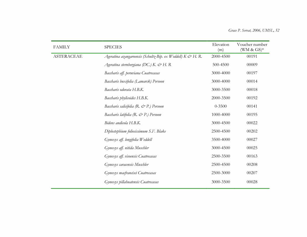
Grace P. Servat, 2006, UMSL, 52
FAMILY SPECIES Elevation (m)
Voucher number (WM & GS)*
ASTERACEAE Ageratina azangaroensis (Schultz-Bip. ex Weddell) K & H. R. 2000-4500 00191
Ageratina sternbergiana (DC.) K. & H. R 500-4500 00009
Baccharis aff. peruviana Cuatrecasas 3000-4000 00197
Baccharis buxifolia (Lamarck) Persoon 3000-4000 00014
Baccharis odorata H.B.K. 3000-3500 00018
Baccharis phylicoides H.B.K. 2000-3500 00192
Baccharis salicifolia (R. & P.) Persoon 0-3500 00141
Baccharis latifolia (R. & P.) Persoon 1000-4000 00195
Bidens andicola H.B.K. 3000-4500 00022
Diplostephium foliosissimum S.F. Blake 2500-4500 00202
Gynoxys aff. longifolia Weddell 3500-4000 00027
Gynoxys aff. nitida Muschler 3000-4500 00025
Gynoxys aff. visoensis Cuatrecasas 2500-3500 00163
Gynoxys caracensis Muschler 2500-4500 00208
Gynoxys macfrancisci Cuatrecasas 2500-3000 00207
Gynoxys pillahuatensis Cuatrecasas 3000-3500 00028
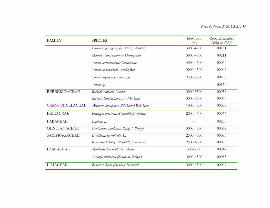
Grace P. Servat, 2006, UMSL, 53
FAMILY SPECIES Elevation (m)
Record number (WM & GS)*
Loricaria ferruginea (R. & P.) Weddell 3000-4500 00161
Mutisia cochabambensis Hieronymus 3000-4000 00211
Senecio torrehuasencis Cuatrecasas 4000-4500 00034
Senecio hohenackeri Schultz-Bip. 3000-4500 00046
Senecio usgarens Cuatrecasas 2500-3500 00196
Senecio sp --- 00150
BERBERIDACEAE Berberis carinata Lechler 3000-3500 00056
Berberis humbertiana J.F. Macbride 3000-3500 00053
CARYOPHYLLACEAE Arenaria lanuginosa (Michaux) Rohrbach 1000-4500 00058
ERICACEAE Pernettya prostrata (Cavanilles) Sleumer 2000-4500 00066
FABACEAE Lupinus sp --- 00239
GENTIANACEAE Gentianella sandiensis (Gilg) J. Pringle 3000-4000 00072
SAXIFRAGACEAE Escallonia myrtilloides L. 2500-4000 00083
Ribes brachybotrys (Weddell) Janczewski 2500-4500 00080
LAMIACEAE Minthostachys mollis Grisebach 500-3500 00247
Satureja boliviana (Bentham) Briquet 3000-4500 00085
LILIACEAE Bomarea dulcis (Hooker) Beauverd 3000-4500 00002

Grace P. Servat, 2006, UMSL, 54
FAMILY SPECIES Elevation (m)
Record number (WM & GS)*
LOGANIACEAE Buddleja aff. montana Britton 2500-4000 00225
MELASTOMATACEAE Brachyotum naudinii Triana 2500-4000 00263
PIPERACEAE Peperomia hartwegiana Miquel 3000-4500 00272
POACEAE*** Stipa ichu (R. & P.) Kunth 1000-4500 NC
Festuca dolichophylla J. S. Presl 3500-4500 NC
Calamagostris rigescens (J. S. Presl) Scribner 3500-4500 NC
POLYGALACEAE Monnina salicifolia R. & P. 1500-4500 00104
POLYGONACEAE Muehlenbeckia nummularia H. Gross 3000-4000 00274
Rumex acetocella L. 2000-4500 00273
ROSACEAE Polylepis racemosa R. &. P. 3000-4500 00172
Polylepis incana H. B. K. 2500-4500 00358
Polylepis sericea Weddell 2500-4500 00277
Polylepis weberbauerii Pilger 2000-4500* 00171
SCROPHULARIACEAE Bartsia bartsioides (Hooker) Edwin 2000-4500 00119
Calceolaria engleriana Kraenzlin 2000-4500 00127
SOLANACEAE*** Salpichroa hirsuta (Meyen) Miers 3000-4500 NC
URTICACEAE Urtica echinata Bentham 3500-4500 00178

Grace P. Servat, 2006, UMSL, 55
FAMILY SPECIES Elevation (m)
Record number (WM & GS)*
VERBENACEAE Duranta mandonii Moldenke 2500-4000 NC
PTERIDOPHYTES Adiantum poeretii Wikstrom --- NC
Melpomene flobelliformis (Poiret) A. R. Sm & R. C. Moran --- 00329
Asplenium haenkeanum (C. Presl) Hieron. --- 00333
Asplenium castaneum Schletcht & Cham --- 00337

Grace P. Servat, 2006, UMSL, 56
CHAPTER TWO
INTRASPECIFIC VARIATION IN THE FORAGING NICHE OF BIRDS ASSOCIATED WITH POLYLEPIS WOODLANDS: THE INFLUENCE OF
LOCAL AND REGIONAL FACTORS
The niche concept has played a central role in ecology for nearly a hundred years,
mainly to gain insights into community organization (Gause 1930, Hutchinson, 1957,
MacArthur 1958, 1965, Connell 1951, MacArthur and Levins 1964, MacArthur and Pianka
1966, Emlen 1966, Levin 1970, Tilman 1982, for a review see Chase and Leibold 2003).
Contemporary theory defines the niche of a species as the requirements for existence in a
given environment (i.e., the n-dimensional hyper-volume niche, Hutchinson 1957) and its
role on that environment (Ricklefs 1997, Chase and Leibold 2003, Naeem 2003), extending
the “Principle of Competitive Exclusion” (Gause 1930, Hardin 1960) to the condition that
only species with sufficiently differentiated niches may coexist within the same community
or environment (for review see Futuyma and Moreno 1988, Chase and Leibold 2003).
Classic niche studies have focused on resource-based, interspecific differences based
on competition theory to determine how two or more species with similar niches can
coexist by partitioning habitats (e.g., Paramecium, Gause 1930; grain beetles, Crombie 1945-
1947, Park 1948), microhabitats (e.g., barnacles, Connell 1951; Dendroica warblers, MacArthur
1958), resources (e.g., algae and terrestrial plants, Tilman 1976, 1982), and foraging heights
(e.g., warblers, MacArthur 1972). Based on these studies, interspecific differences in niche
partitioning were inferred to influence the ecological outcomes of communities (see review
in Chase and Leibold 2003, but see Hubbell 2001). However, communities include

Grace P. Servat, 2006, UMSL, 57
conspecifics as well as other species, and intraspecific differences in the niche also have
ecological and evolutionary consequences for the species and communities involved (Van
Valen 1965; Grant 1967, 1979; Roughgarden 1972, 1974; Bolnick et al., 2003). Moreover, as
natural selection operates at the level of the individual, the importance of including
measures of intraspecific variation in species’ niche has been seen with renewed interest in
studies of local adaptation, adaptive radiation, and ecological speciation (e.g., Losos 1990,
Throwbridge 1991; Dayan and Simberloff 1994, Linhart and Grant 1996, Reznick and
Travis 1996, Nagy and Rice 1997, Bronikowski 2000, Olson and Uller 2003, Bolnick et al.
2003, Scott et al. 2003, Meiri et al. 2005).
Intraspecific variation in the niche is likely affected by local differences in abiotic
and biotic factors (e.g., temperature, Houlahan et al. 2000; Shuter et al. 1980; Magnusson et al.
1979; elevation, Berven 1982, 1990; microclimate, Martin 1998, 2001; habitat diversification,
Robinson and Wilson 1994; prey distribution, Ehlinger and Wilson 1988; intraspecific
competition, Smith 1990; predation, Martin 1993, 1998, Gilliam and Fraser 2001, Werner
1984). Furthermore, the niche may also be influenced by a complex and dynamic set of past
and present factors acting on different spatial and temporal scales as shown in a variety of
studies across taxa (e.g., Darwin’s finches, Grant 1986; Caribbean Anolis lizards, Losos 1990,
Losos et al. 1998, 2003; stream fishes, Angermeier and Winston 1998; desert rodents, Kelt
1999; plants in calcareous grasslands, Pärtel and Zobel 1999).
Quantitative approaches to the study of interspecific and intraspecific niche
variation are based on measures of its components (Roughgarden 1972, 1974, Bolnick et al.
2003): breadth and plasticity. Niche breadth is defined as the number of resources used by a
particular species and measures if the species is a specialist or generalist relative to other

Grace P. Servat, 2006, UMSL, 58
community members or species in a clade (Futuyma and Moreno 1988, Mac Nally 1995 and
references therein). A specialist uses a relatively limited fraction of the range of available
resources (i.e., narrow niche breadth, Fig. 2.1 A) while a generalist uses a relatively large
fraction of the resources available (i.e., broader niche breadth, Fig. 2.1 A) without regard for
underlying mechanisms that determine how the species manages to identify, select, and
capture a particular resource or the fitness effects on the focal species (Bolnick 2003; e.g.,
Sherry 1984, Mac Nally 1995). Niche plasticity evaluates how restricted or plastic is the
niche of a species within and across populations (Fig. 2.1 B) (Mac Nally 1995, Roughgarden
1972, 1974; Bolnick et al., 2003). The term restricted applies to the conditions under which
intraspecific regularities in the niche might be maintained, and the term plastic applies when
niche regularities within and across populations break down (Sherry 1990, Price 1991, Price
and Jamdar 1991, Richman and Price 1992, Holbrook and Schmitt 1992, Forstmeier et al.
2001). Thus, a species may have a restricted (or plastic) niche, even if its niche breadth is
narrow (specialist) or wide (generalist) provided if it remains consistent across populations
throughout its distribution (i.e., restricted populations may be made up of individual
generalists or, equally plausibly, from a variety of individual specialists) (Fig. 2.1 C). Both
components provide complementary information for comparisons at different spatial scales
and levels of organization (e.g., populations, species, and communities).
In this study, I examined intraspecific niche variation (or lack thereof) of nine
species of forest interior, arboreal, arthropod-feeding birds (hereafter, insectivorous) of the
Polylepis (Rosaceae) community, a high elevation system of the Andes. I focus the study
from a behavioral perspective because foraging behavior (along with physiology and
morphology) is crucial to adapt to new habitats and, it is an important target of selection

Grace P. Servat, 2006, UMSL, 59
(e.g., Sherry 1985, 1990, Morimoto and Wasseman 1991, Losos 1990). In addition, at high
elevation systems, arboreal-insectivorous birds spend most of their time and effort using
several substrates and maneuvers to search and obtain food, so it is likely that the way in
which individuals forage influences their performance, as natural selection should favor
those strategies that maximize fitness or some proxy of fitness (e.g., rate of resource
acquisition, production of offspring). Specifically, I quantify the niche breadth and plasticity
based on measures of a) microhabitat use (Levin’s index), and b) foraging categories used
(measured by plotting maneuvers and substrates in multivariate space, cf. Mac Nally 1995).
Measures of variation in breadth and plasticity were analyzed in light of variation in
ecological factors across Polylepis woodlands. I focus on three factors that may vary locally:
food resources, floristic composition, and vegetation structure because these have been
reported to influence the niche of species intra and interspecifically (Wiens 1989, Werner
and Sherry’s 1987, Lewontin 1987, Cadle and Greene 1993, Cornell and Lawton 1992,
Latham and Ricklefs 1993, Francis and Currie 1998, Huston 1999). Fluctuations in the
relative abundance, availability of alternative food types, spatial relationship among
resources, attributes of resources such as palatability and/or hardness have been reported to
influence: a) the relative abundance of individuals in populations or communities; b)
seasonal migration (e.g., Rabenold 1978, 1979, 1980, Recher et al. 1983, 1985, Recher and
Holmes 1985, Loiselle and Blake 1991, Blake and Loiselle 1991); c) opportunistic
aggregation in areas of high food abundance (e.g., Brush and Stiles 1986); and d) partition of
food resources (e.g., Holmes and Shultz 1988, Holmes and Pitelka 1968), foraging substrates
(e.g., Hejl and Verner 1990), and strata. Besides food resources, variation in floristic
composition is expected to provide a set of opportunities and constraints that may result in

Grace P. Servat, 2006, UMSL, 60
close associations between birds and particular plant species. In addition, variation in plant
species composition could affect foraging ecology of birds because of differences in the
spatial arrangement of leaves, branching patterns, and other parameters of plant species’
architecture (e.g., Holmes and Robinson 1981, Franzeb 1983, Morrison et al. 1985, Tomoff
1974, James and Wamer 1982, Rotenberry 1985, Wiens and Rotenberry 1981, MacNally
1990, 1995). Vegetation structure in forests with high diversity of plant species may also be
more complex in terms of strata (i.e., number of layers in understory, subcanopy, and
canopy) and life forms (i.e., shrubs, small trees, large trees) and, thus, provide more
substrates or microhabitats in which to forage when compared to low diversity woodlands
(Holmes et al. 1979, Robinson 1981, Robinson and Holmes 1984). Some characteristics of
habitat structure known to affect foraging ecology of birds are the number or types of
substrates available (Jackson 1979, Fitzpatrick 1980, Greenberg and Gradwohl 1980) and
forest physiognomy (Robinson and Holmes 1984, Whelan 1989, in Mac Nally 1995, Maurer
and Whitmore 1981, Sabo and Holmes 1983). Moreover, regional factors, such as
biogeography (i.e., the presence of barriers that have an effect on species dispersal), may
influence the niche of a species within and across populations (e.g., Wiens 1989, Werner and
Sherry’s 1987, Lewontin 1987, Cadle and Greene 1993, Cornell and Lawton 1992, Latham
and Ricklefs 1993, Francis and Currie 1998, Huston 1999). The relative importance of
regional factors (i.e., biogeography) in explaining foraging niche variation is indirectly
assessed in this study by selecting a series of Polylepis woodlands nested within three distinct
biogeographic regions of the Peruvian Andes.
The goals of the present study are 1) to measure the extent of variation in two
foraging niche components (breadth and plasticity) of nine species of arboreal-insectivorous

Grace P. Servat, 2006, UMSL, 61
birds in light of local conditions (e.g., food resources availability, floristic composition, and
vegetation structure) in a series of Polylepis woodlands nested within three distinct
biogeographic regions, and 2) determine the relative importance of local and/or regional
factors in explaining niche patterns.
The hypotheses of the study are: 1) Variation in local and/or regional factors within
and across woodlands influences intraspecific measures of the foraging niche (breadth and
plasticity) of birds associated with the Polylepis community (“local/regional factors
hypothesis”). Support for the hypothesis could result in two non-mutually exclusive
scenarios: a) If the foraging niche varies in response to local factors, niche breadth and
plasticity will track one or more local factors (i.e., abundance of food resources, floristic
composition or vegetation structure); b) If niche varies regionally, I expect differences in
species niche breadth and plasticity across regions but not among forests within region. 2)
Intraspecific measures of foraging niche of birds are static and do not reflect variation in
local or regional factors within or across Polylepis woodlands (“historical/morphological
factors hypothesis”). If foraging niche breadth and plasticity of bird species do not vary
within and across populations, despite variation in local and regional factors, history of taxa
and/or morphology likely constrains the foraging niche of the species.
METHODS
Study system
Throughout the high Andes from 3400 to 4600 m, Polylepis woodlands are typically
found close to streams or as small patches in canyon gorges on slopes and cliff-edges; these

Grace P. Servat, 2006, UMSL, 62
forests in Peru are surrounded by Puna grasslands. The Polylepis community is dominated by
Polylepis (Rosaceae) trees and characterized by high levels of endemism in flora and fauna
and thus, it is of great interest from evolutionary and ecological perspectives (Fjeldså and
Krabbe 1990, Fjeldså 1992a, b, c; 1993). Polylepis woodlands are scattered in different
biogeographic regions throughout the Andes, offering discrete units of study (i.e., local
communities) within a historical framework. Moreover, the flora and fauna are relatively
simple when compared to more species-rich woodlands at lower elevations, allowing
comprehensive studies at different scales (local, regional) and levels of organization (species,
populations, communities).
The patchy occurrence of Polylepis woodlands is attributed to microclimatic and
physiological requirements (Weberbauer 1945, Troll 1959, 1968, Koepcke 1961, Walter and
Medina 1969, Simpson 1979, 1986, Vuilleumier 1984, Rauh 1988). Yet it also has been
suggested that these woodlands are relicts of a once more widespread habitat during the
Pleistocene (i.e., 10,000-20,000 years ago) (Ellenberg 1958, Beck and Garcia 1991, Fjeldså
1992a, Hensen 1993, Kessler 1995).
Regional settings
The present study was conducted in three separate regions of the Peruvian Andes:
Cordillera Blanca, C. Occidental, and C. Vilcanota (Fig. 2.1), areas that have been proposed
as distinct glacial Pleistocene refuges for a number of taxa (Fjeldså 1992a, 1993, Fjeldså and
Kessler 1996) and as different biogeographic regions (Berry 1982, Koepcke W. 1961,
Koepcke M. 1961, Lamas 1982, Fjeldså 1992 a, Simpson 1975, Smith 1988). In more humid
regions Polylepis woodlands often have some dense, shady sections with deep fertile soil and

Grace P. Servat, 2006, UMSL, 63
lush vegetation of herbs between moss-covered rocks. Trees are heavily laden with mosses,
vines (e.g., Bomarea, Mutisia, Passiflora, and Salpichroa) and mistletoes (i.e., Tristerix); bushes and
trees of Gynoxys (Asteraceae) are often interspersed with Polylepis.
Very few climatic data are available for the study regions, but high Andean systems
are generally characterized by small annual variation in mean temperature while daily
patterns may go from freezing temperatures during the night (-3 º C) to high daytime
temperatures (24º C) (Sarmiento 1986). Precipitation in tropical mountains occurs when the
Inter-tropical Convergence Zone (ITCZ) is at its southernmost point (40°- 45° latitude
south). Variation in the position of the ITCZ drastically affects rainfall in the mountains
resulting in the wet (December - April) and dry seasons (May - November). However,
precipitation patterns during the wet season tend to be more complex and variable within
regions than across regions due to exposure to winds and orography (Lenters and Cook
1995).
Local settings
For this study, I selected four Polylepis woodlands within each of the three regions
that matched the following criteria: 1) sites were above 3500 m where Polylepis forms distinct
woodlands surrounded by Puna vegetation (Lamas 1982, Kessler 1995); and, 2) woodlands
were presumably large enough (> 50 ha) to maintain populations of selected bird species.
The woodlands selected for the present study ranged in size from 50 - 300 ha (Table 2.1);
and the dominant Polylepis species occurring in each forest were: 1) C. Blanca: Aquilpo and
Ishinca (P. weberbauerii), Morococha and Llanganuco (P. sericea); 2) C. Occidental: Yaui and

Grace P. Servat, 2006, UMSL, 64
Quichas (P. weberbauerii); Maticuna and Japani (P. incana); and 3) C. Vilcanota: Yanacocha,
Sacsamonte, Pumahuanca, Quenuamonte (P. racemosa).
General study design
I collected data in 12 Polylepis woodlands from May - December 1997 (foraging
niche of birds, floristic composition, and vegetation structure) and returned to the same
woodlands in May - October 1998 (foraging niche of birds, arthropod resources) (Table 2.1)
which corresponded to the dry season and beginning of the rainy season. In all cases, I used
a hierarchical sampling design with the four woodlands nested within each of three regions.
In each Polylepis forest, I collected data on foraging niche of birds and abundance of
arthropod resources in two sets of four 100 x 10 m transects placed 50 m apart from each
other. The last transect from the first set was separated by at least 500 m from the first
transect of the second set (hereafter the two sets of transects will be referred as plots). I
took data on floristic composition and vegetation structure in two 20 x 5 m belts embedded
within each transect. To examine variation in local factors such as arthropod abundance,
floristic composition and vegetation structure among woodlands, I used plots within
woodlands as replicate units (Chapter I).
Study birds
Approximately 112 bird species are regularly found in Polylepis woodlands of the
Andes of Peru. This number includes opportunistic visitors from lower montane forests
and surrounding grasslands, bogs, and wetlands (Fjeldså 1992 a, 1997). Of these 112 species,
at least 22 are found in Polylepis woodlands as regular breeding residents (= associated

Grace P. Servat, 2006, UMSL, 65
species) (Fjeldså and Krabbe 1990, Fjeldså 1992 a, b, c, 1993). I studied nine species of
forest-interior, arboreal, insectivorous birds associated with the community: Oreomanes fraseri,
Cranioleuca baroni (or its ecological replacement C. albicapilla), Xenodacnis parina, Leptasthenura
pileata (or its ecological replacement L. xenothorax), L. yanacensis, Mecocerculus leucophrys, and
Octhoeca rufipectoralis (Table 2.2) (cf. Fjeldså and Krabbe 1990, Fjeldså 1992 a, b, c).
I made observations of actively foraging birds using the Remsen and Robinson
(1990) classification of foraging behavior. I quantified microhabitats, defined here as parts
of the habitat where individuals forage, which in this case, are given by the combination of
plant species and substrate used by birds (e.g., Polylepis bark, Gynoxys foliage), and maneuvers
(prey capture attempts, e.g., glean, probe) used by individual birds. At each forest, I made
observations throughout the day, most of which occur between 0800-1200 hrs, and 1400-
1700 hrs, for four and six consecutive days in 1997 and 1998, respectively. I systematically
walked transects and moved from one foraging bird to another using focal-animal sampling
(Altmann 1974); observations of foraging birds were audio-recorded, or videotaped when
possible. I obtained foraging observations (i.e., maneuvers and microhabitats used) from a
minimum of 10 individuals of each species in each of the 12 Polylepis woodlands. For each
individual, the average length of continuous foraging time recorded was 180 seconds
(individuals observed less than 180 seconds were excluded from analysis), which was later
divided into 60-second sequences. As the number of continuous observations obtained for
each species was highly variable in each Polylepis forest. I first chose 20 individuals and
randomly selected one 60-second sequence from each continuous observation. This
procedure allowed me to lessen biases that may exist due to lack of independence of
observations (i.e., foraging maneuvers and microhabitat use may depend on previous

Grace P. Servat, 2006, UMSL, 66
behaviors). For a few sites, however, this was not possible because of small sample size, in
which case I used all sequences collected. I combined foraging maneuvers and
microhabitats for each sequence into categories (Fig. 2.2). Some rare foraging combinations
(those used 1 or 2 times in only one of the 12 localities) were excluded from analyses.
The main data set consisted of columns that represented 25 foraging categories and
1480 rows corresponding to each individual/species/forest (1480 rows instead of 1600 due
to the absence of species at some sites). Counts of the total number of times that each
foraging category was used by each individual in the 60-second sequence (hereafter =
individuals) fill the cells of the matrix. From these data, I constructed different matrices for
analyses.
Variation in local factors
I measured local food availability (i.e., types and abundance of arthropods in
different microhabitats), floristic composition (i.e., plant species richness and abundance),
and horizontal and vertical vegetation structure, as factors that can shape the foraging niche
of birds.
Food resources.- Food resources may affect how birds move through the habitat and
how they encounter and capture prey. To measure the abundance of arthropods, the
primary food resource of study birds, I identified microhabitats (i.e., “patches” containing
food resources that can be discriminated by an individual; Morris 1987 in Mac Nally 1995)
as the unit of sample. Microhabitats were defined by the combination of dominant plant
species (i.e., Polylepis, Gynoxys, Tristerix) and substrates used (i.e., bark, foliage), except for the
moss attached to the branches of Polylepis trees (that included many epiphytic species). I

Grace P. Servat, 2006, UMSL, 67
quantified arthropods by focusing on discrete microhabitats used by foraging birds (based
on preliminary studies): Polylepis bark; Polylepis, Gynoxys, and Tristerix foliage; and moss. Due
to the structural differences among microhabitats, arthropod sampling varied. I sampled
arthropods from the trunk of Polylepis trees by removing a 20 x 20 cm quad, 150 cm above
the ground. Polylepis, Gynoxys, and Tristerix foliage (twigs with leaves) were sampled by
clipping three or four 30-cm terminal twigs selected randomly from the lower to middle
crown of trees or shrubs. To sample arthropods from moss, I removed a 20 x 20 cm quad
of moss from branches (150 cm from the ground). In every case, I sampled 24 Polylepis trees
(or Gynoxys shrubs or trees and Tristerix plants) equally divided between the two plots and
calculated arthropod abundance per microhabitat across Polylepis woodlands. Samples of
bark, foliage, and moss were placed in plastic bags and weighed using a “Pesola” scale. In all
cases, attempts were made to sample similar amounts of bark, moss, and foliage per sample
(ca. 50 gm). Arthropods were removed using tweezers, counted and preserved in 70 %
alcohol. Arthropods with aposematic coloration, low occurrence (< 5 individuals per
microhabitat), or less than 2 mm length, were excluded from the present study as they likely
do not constitute prey for birds due to low acceptability or detectability (Wolda 1990, Servat
1995).
Floristic richness and composition.- Plant species richness and composition at each
Polylepis forest was measured by counting and identifying trees (>10 cm dbh) and “woody
stems” (<10 cm dbh) found in the forest interior (i.e., 50 m away from edge of the plot, see
study design above). The data obtained were used to build a matrix consisting of 12 Polylepis
woodlands (rows) by 50 plant species (columns), cells were filled with the total number of
individuals found.

Grace P. Servat, 2006, UMSL, 68
Vegetation structure.- I divided vegetation structure variables into those that represent
“horizontal complexity” (i.e., the distribution of tree size classes, density of vegetation, and
tree diameter) and those that represent the “vertical complexity” of the habitat (i.e., the
diversity of vegetation heights and density of foliage at those heights, vertical layers:
understory, subcanopy and canopy) (e.g., MacArthur et al. 1962, Robinson and Holmes
1984, Rotenberry 1985, MacNally 1990, 1995).
1. Vertical structural variables
a. Mean tree height (HEIGHT).- I measured trees using a telemetric graduated pole (12
m, Hastings Telescoping Measuring Rod).
b. Foliage height density (FHDEN).- I took measurements of foliage height density,
with a telemetric graduated pole, along "vertical" transects every 20 m along the two sets of
100 m transects (see study design). The number of times vegetation “intersected” the pole
in a radius of 25 cm was recorded at the following intervals: 0-2 m (FHDEN1), > 2-6 m
(FHDEN2), and > 6-10 m (FHDEN3). Vegetation contacts were summed within each
interval across points and then divided by total contacts across all heights to obtain a
proportion of foliage density occurring within different heights.
2. Horizontal structural variables
a. Tree size classes (DBH).- I measured diameter at breast height for each tree
encountered, regardless of species identity, and assigned them to one of three size
categories: > 10-20 m dbh (DBH1), > 20-30 m dbh (DBH2), and > 30 cm dbh (DBH3). For
each local factor, I used data obtained in plots as replicates in the models. All variables were
tested for normality, and equality of variances.

Grace P. Servat, 2006, UMSL, 69
b. Total basal area (TBA).- Total basal area was measured to describe tree coverage.
TBA was calculated by converting measures of dbh (i.e., distance at breast height) to circular
area, estimating proportional basal area for each tree species and adding all tree basal areas
for each plot.
c. Tree (TD) and shrub density (SD).- I measured tree and shrub density by counting the
number of trees (> 10 cm dbh) or woody stems (> 50 cm height and < 10 cm dbh) per plot
and dividing the total by the sampled area to obtain density values.
Regional factors.- Regional factors in this study refer to history of the environment (i.e.,
biogeography) and are inferred by the study design in which four independent Polylepis
woodlands were nested within each biogeographic region.
Data analysis
To determine if foraging niche of each of the focal species vary across and within
populations, I measured breadth and plasticity.
Niche breadth.- The niche breadth is a measure of variability in the extent to which a
species uses resources (Feinsinger et al. 1981, Gotelli and Graves 1996). In this study,
measures of breadth indicated the degree to which microhabitat exploitation was evenly
spread among alternative states. I used Levin’s non-conformance niche breadth (Levins
1968) given by: 1/Σi (pi)2 where pi is the proportion of resource items (microhabitats) in state
i out of all items used by the population. For each species, low values of niche breadth
imply that a small number of potential microhabitats were used (i.e., specialist) across
populations, whereas relatively high values indicated a large number of microhabitats were

Grace P. Servat, 2006, UMSL, 70
used more evenly (i.e., generalist). It is important to note that values of niche breadth were
not absolute, but relative values across species and populations.
To analyze niche breadth, I selected one species at a time and calculated the niche
breadth, based on the foraging microhabitats used by each individual in a population
(replicates). I compared variation in niche breadth values (dependent variable) across
Polylepis woodlands and regions of the Andes (as the main effect and nested factors
respectively) using Hierarchical Multivariate Analysis of Variance (SPSS, Version 10) to
separate out the variation attributed to regional (i.e., among regions), or local niche breadth
(i.e., among woodlands within regions) by levels of significance. I followed the analysis with
Post-hoc Tukey (HSD) test when appropriate. Based on statistical significance of niche
breadth, and the observed mean (and SD), I categorized species into specialists (if mean
niche breadth was relatively narrow, variation is small and no significant differences are
detected across woodlands and regions), or generalist (if mean niche breadth was relatively
broad, highly variable and significant differences were found across woodlands and regions
of study).
Niche plasticity.- Plasticity is a measure of the foraging niche consistency within and
across populations of the same species. Thus, species could be restricted if intraspecific
regularities in the niche are maintained, or plastic if niche regularities within and across
populations break down. In this study, bird species may have a restricted (or plastic) niche,
even if its niche breadth is narrow (specialist) or wide (generalist) as long as it remains
regular across populations (i.e., restricted populations may be made up of individual
generalists or, equally plausibly, from a variety of individual specialists) (Fig. 2.1 C).

Grace P. Servat, 2006, UMSL, 71
I determined foraging plasticity for each bird species across Polylepis woodlands and
regions by identifying the “spatial position” that each individual occupies in the population.
I employed PC-ORD Version 4 (McCune and Mefford 1999) to do Bray Curtis ordination. I
selected Sorensen’s percent dissimilarity as a measure of distance between points (individual
birds). This index is commonly used with ecological data because it retains sensitivity in
heterogeneous data sets and gives less weight to outliers (McCune and Mefford 1999). I
used the variance regression method for end point selection and Euclidean distance for axis
projection geometry (Beals 1984, Greig-Smith 1983, McCune and Mefford 1999). The
arrangement of points (i.e., each individual position along the first two axes) obtained from
the ordination represents the linear combinations of all foraging categories used by within
and across populations. Thus, I selected one bird species at a time, and for each population,
I used the scores of all individuals along the first two axes from the previous ordination (see
above) to calculate the population centroid. To obtain a single value for the two-
dimensional position of each individual, I used the algebraic expression a2+b2=c2; where a is
the difference between the location of the centroid and the location along the first axis of
each individual within the population, b is the difference between the location of the
centroid, and the location along the second axis of individuals in the population, and
consequently c represents the distance to the centroid. For each population, I calculated the
mean c value and the standard deviation; or the square root of the sum of the position
divided by the number of observations minus one [SD= √ Σc2/ (n-1)] to represent niche
plasticity.
To analyze data I used the c value (dependent variable) of individuals in each
population as replicates in Hierarchical Multivariate Analysis of Variance (SPSS, Version 10)

Grace P. Servat, 2006, UMSL, 72
to separate out the variation attributed to the main effect (i.e., among regions of the Andes),
or nested factor (i.e., among woodlands within regions) by levels of significance. I followed
the analysis with Post-hoc Tukey test when appropriate.
Variation in ecological factors
To determine if food resources, floristic composition richness, and vegetation
structure vary locally and/or regionally I first analyzed each factor independently.
Food resources and floristic composition.- I used rarefaction to analyze variation in richness
of food resources (arthropods/microhabitat) and plants using plots as replicates across
Polylepis woodlands. Rarefaction uses probability theory to derive the expected mean and
variance of species richness for a sample of a given size (Hurlbert 1971, Heck et al. 1975,
Gotelli and Graves 1996). I used Ecosim (Gotelli and Entsminger 2004) to obtain the
expected mean richness and variance (of plants and arthropods, independently) while
controlling for the number of individuals (Sanders 1968 in Gotelli and Graves 1996). The
process was simulated 1000 times specifying the number of individuals that are randomly
drawn from each sample.
Vegetation structure.- To analyze variation in vegetation structure within and across
Polylepis woodlands, I used the mean and SD for each of the 11 variables measured (plots as
replicates). Local and/or regional variation in food resources, floristic composition, and
vegetation structure were tested using hierarchical MANOVA models to interpret foraging
niches. As before, hierarchical MANOVA tests separated out the variation attributed to
regional (i.e., among regions) or local scales (i.e., among woodlands within regions) by levels
of significance.

Grace P. Servat, 2006, UMSL, 73
After the independent analyses of local factors, I determined the relative importance
of local and regional factors in the foraging niche of birds. I used Mantel Tests (Mantel 1967,
Sokal and Rohlf 1995, Burgman 1987) to identify the relative effect of local and regional
factors in explaining patterns of foraging niche of each bird species across woodlands. I
used seven independent models (one for each bird species) and built distance matrices to
obtain a measure of resemblance (= Sorensen’s dissimilarity index) in foraging niche for
each possible pair of populations (response variable), and a measure of resemblance in food
resources, floristic composition, vegetation structure, region, and geographic distance
(predictor variables) for each possible pair of sites. Mantel test uses a regression approach to
evaluate the null hypothesis of no relationship between two distance matrices and basically
determined if pair-wise population differences in foraging categories could be explained by
pair-wise differences in any of the factors measured. I customized distance matrices for each
bird species, since some of the variables measured (i.e., food resources) were used differently
by different bird species. Each model consisted of the following distance matrices:
a. Foraging matrix.- To evaluate the relationship between site similarities in food
resources used and foraging behavior of species I selected one species at a time from the
main data matrix (see above), and summed up all counts for each foraging category used
across all individuals within a population. This resulted in a matrix of 7-12 populations
(based on the presence of the species at a site) x 6-11 foraging categories (11 was the
maximum number of categories used by any one species from the total 25).
b. Food resources matrix.- The relationship between similarities in food resources used
and foraging behavior of species was evaluated using the total number of arthropods
(corrected by weight of bark, foliage, and moss) to build a forest x microhabitat matrix (7-12

Grace P. Servat, 2006, UMSL, 74
sites x 3-5 microhabitats used). Data on food resources were customized for each bird
species based on which foraging microhabitat(s) used, or if these were present at a site. For
instance, in the Cranioleuca species I only included data on arthropod abundance from bark
and foliage (as this species uses these microhabitats to feed) from localities where the
species occurred. Customized matrices for O. fraseri included only abundance of arthropods
found in bark, while for Leptasthenura species I used arthropod data from foliage and bark
microhabitats, and for X. parina I used Polylepis, Gynoxys and Tristerix foliage. For the two
flycatchers, M. leucophrys and O. rufipectoralis, I used arthropod abundance from Polylepis
foliage because these likely constitute most of the flying prey caught by the birds during
aerial maneuvers.
c. Floristic composition matrix.- To evaluate the relationship between site similarities in
floristic composition and bird species foraging behavior, I built a forest x plant species
matrix (12 sites x 50 plant species) in which the presence (“1”) or absence (“0”) of each
plant species filled the cells of the matrix.
d. Vegetation structure matrix.- To evaluate the relationship between vegetation
structure and foraging niche of birds, I built a forest x vertical structure variables matrix (12
sites x 4 variables) and a forest x horizontal structure variables matrix (12 sites x 5 variables)
in which a single measure for each variable (averaging data from the two plots, see study
design) filled the cells of the matrix.
e. Region matrix.- A “regional distance matrix” was built by examining each forest pair
and scoring “0” if they belonged to the same region and “1” if they differed (Sokal and
Rohlf 1995); this regional variable was added as another predictor in the Mantel test.

Grace P. Servat, 2006, UMSL, 75
Distance matrices of predictor variables matched the size of the bird matrix; that is,
data on arthropod abundance, floristic composition, vegetation structure, and region were
not included at sites where bird species were absent. Except for the “regional distance
matrix”, I relativized original matrices by “the norm” (Greig and Smith 1983) using rows or
columns to make categories comparable for each population or site; and used Sorensen’s
percent dissimilarity as a measure of distance between points (populations or sites).
The models were run using Permute! version 3.4, alpha 9 (Legendre et al. 1994), a
special version of Mantel test, that allows for several predictor variables to be tested over one
response variable generating partial regression coefficients and the associated permutation
probability for each variable. I used stepwise regression, a backward elimination procedure,
and performed 999 permutations of the original matrix to determine the significance
probability of the observed relationship among the response and predictor variables.
RESULTS
Proportional use of foraging categories
Insectivorous birds associated with Polylepis woodlands differed in the relative
proportion of maneuvers and microhabitats used across sites and regions (Fig. 2.3 a-g).
Some species, for instance, O. fraseri, foraged proportionally more (> 60 %) on the bark of
Polylepis trees, using to a lesser extent other microhabitats (Fig. 2.3 a). Maneuvers used by O.
fraseri included several hanging postures (up, down, sideways, upside down) to probe inside
the multi-layered bark, or to glean arthropods from the surface. Other bark-foragers such as
C. baroni (in C. Blanca and C. Occidental) and C. albicapilla (in C. Vilcanota) used

Grace P. Servat, 2006, UMSL, 76
proportionally more Polylepis bark, but also included regularly other microhabitats such as
dead branches hanging in the understory or attached to trees, tree surfaces covered by moss,
and Polylepis foliage (Fig. 2.3 b). Comparatively, Cranioleuca species use more surface gleaning
(hover-glean, sally-glean, and reach-glean) than O. fraseri (Fig. 2.3 a, b).
More than 80 % of observations of L pileata and its ecological replacement L.
xenothorax were foraging in Polylepis foliage (Fig. 2.3 c). The two species used many hanging
postures to glean prey from the surface of twigs and leaflets of Polylepis trees, but
interspecific differences were also observed. For instance, at some woodlands L. pileata
foraged more in shrubs in the understory than L. xenothorax (e.g., 30 % in Quichas, Fig. 2.3
c), while L. xenothorax used relatively more Polylepis bark surfaces than L. pileata (e.g., 25 % in
Sacsamonte and Pumahuanca, Fig. 2.3 c). Moreover, the proportional use of microhabitats
varied across populations as well (Fig. 2.3 c). The third Leptasthenura species, L. yanacensis,
differed from the other two in the use of several foraging microhabitats (i.e., dead branches,
Polylepis and Gynoxys foliage, moss, Polylepis bark, shrubs, and ground, Fig. 2.3 d). A similar
pattern was observed in the other foliage gleaner, X. parina, that used a variety of
microhabitats for foraging (Gynoxys, Polylepis, and Tristerix foliage) (Fig. 2.3 e).
Species that capture flying insects either flycatching or hover-gleaning such as M.
leucophrys could vary in the proportional use of foraging categories and strata (i.e., understory,
canopy) used across woodlands. For instance in Aquilpo and Llanganuco, M. leucophrys
flycatch or hover-gleaned relatively more often on prey on the surface of shrubs and Polylepis
foliage, while in the remaining sites M. leucophrys was mostly observed flycatching in the
canopy (Fig. 2.3 f). The other flycatcher, O. rufipectoralis, used relatively more sally-sit and
Grace P. Servat, 2006, UMSL, 77
flycatching to catch flying insects swarming in the air or on the surface of shrubs in the
understory (Fig. 2.3 g).
Foraging niche breadth: specialist or generalist?
Throughout Polylepis woodlands, the use of foraging microhabitats by some bird
species was maintained while some others vary locally and/or regionally as reflected by
niche breadth values. Based on breadth variation (or lack thereof), O. fraseri and L.
xenothorax are considered specialists because they present relatively narrower niches that did
not vary significantly across populations (Fig. 2.4 a, c, Table 2.3). Most bird species in the
study were generalists in the use of foraging microhabitats, as evidenced by the relatively
broader niche breadth. From these, M. leucophrys and L. pileata (Fig. 2.4 c, f, Table 2.3) were
consistently broad in microhabitat use (i.e., no statistically differences in niche breadth
across populations and/or regions), while C. baroni, C. albicapilla, L. yanacensis, X. parina, and
O. rufipectoralis, varied in niche breadth across populations or regions (i.e., there were
statistical differences in niche breadth values) (Fig. 2.4 b, d, e, g, Table 2.3). In general,
intrapopulation variation in microhabitat use is observed in specialists and generalists’
species (as reflected by SD values) (Fig. 2.4 a-g, Table 2.3).
Foraging niche plasticity: restricted or plastic?
Bird species had different patterns of niche plasticity across populations, as
represented by the position of the c value obtained in the ordination (see methods). For
instance, O. fraseri, L. pileata, L. yanacensis, and X. parina did not show significant differences
in position across Polylepis woodlands, suggesting restriction in the foraging niche (Fig. 2.5 a,

Grace P. Servat, 2006, UMSL, 78
c-e), whereas populations of C. baroni/albicapilla, L. xenothorax, M. leucophrys and O.
rufipectoralis differed significantly in position across populations, suggesting plasticity in the
foraging niche (Fig. 2.5 b, c, f, g).
Based on niche breadth values and foraging plasticity, insectivorous bird species
associated with Polylepis woodlands presented four strategies: a) Specialist-restricted, b)
Specialist-plastic, c) Generalist-restricted, and d) Generalist-plastic (Table 2.4).
Variation in ecological factors
Food resources abundance.- Abundance of arthropods in Polylepis bark, moss, and
Polylepis foliage differed significantly across woodlands (Table 2.5) while Gynoxys and Tristerix
foliage were not significantly different in arthropod abundance across woodlands (Table
2.5). Regional differences in food resources were also found for Polylepis bark, moss, and
Gynoxys foliage. Basically, C. Blanca had fewer arthropods in moss and Gynoxys foliage, while
C. Vilcanota had fewer arthropods in Polylepis bark (Table 2.5).
Arthropods in the bark of Polylepis trees were more abundant when compared with
other microhabitats, excluding the humidity-dependent moss (Servat unpub.). In addition,
Polylepis bark had a distinctive set of arthropods composed by free-living and weaving
spiders, Pseudoscorpionida, and Dermaptera, which likely use the layers of Polylepis bark as a
refugee that protects them against desiccation, a major problem for species at high
elevations (Irons et al. 1993, Lencioni 2004). The other microhabitats included in the study
were pretty distinctive in terms of prey (Servat unpub.), however not all microhabitats were
present at each forest. Based on the presence/absence of microhabitats across Polylepis

Grace P. Servat, 2006, UMSL, 79
woodlands, I considered, Polylepis bark and foliage predictable microhabitats, while Gynoxys,
moss, and Tristerix were unpredictable across forests.
Floristic composition.- Polylepis woodlands contained a total of 50 plant species in 31
genera and 24 families (Servat, Chapter I). Plant species richness differed significantly across
Polylepis woodlands (Table 2.6), with more species found in Llanganuco (average 12 plant
species/100 individuals), Morococha (average 8 species /100 individuals) (C. Blanca), and
Yanacocha (average 12 species/100 individuals) (C. Vilcanota) than in other forest sites
(Table 2.6). Total number of species and individuals also differed among regions, with C.
Occidental (the richest region), contributing to these differences (Table 2.6).
Vegetation structure.- Horizontal structure variables (i.e., TBA, SD, DBH2, and DBH3)
differed significantly across woodlands with exception of the number of small size trees
(DBH1 > 10-20 cm dbh), and tree density (TD) that remain similar in all forests (Table 2.7).
Regional differences were also found in all variables, except for the number of smaller and
larger categories of tree sizes (DBH 1 > 10-20 cm, DBH3 > 30 cm, respectively) (Table
2.7). Basically, woodland differed in the basal area that Polylepis trees occupy (e.g.,, Aquilpo,
Yanacocha, and Yaui had more tree basal area than Llanganuco, Maticuna, Japani and
Pumahuanca woodlands, Table 2.7). Vertical structure variables (i.e., HEIGHT, FHDEN1,
FHDEN2, and FHDEN3) were significantly different across woodlands and regions (Table
2.8).
Local and regional factors and foraging of insectivorous birds
In five of the seven models tested using Permute! (i.e., L. pileata/L. xenothorax, C.
baroni/C. albicapilla, O. rufipectoralis, X. parina and M. leucophrys), site similarities in foraging

Grace P. Servat, 2006, UMSL, 80
ecology of insectivorous birds of Polylepis woodlands were partially explained by site
similarities in food resources, accounting for 10 to 30 % of the variance observed (Table
2.9). For X. parina, site similarities in food resources (R2 = 0.26), floristic composition
(Partial R2 = 0.26), and region (Partial R2= 0. 20) partially explained site similarities in
foraging ecology (Table 2.9). In L. pileata/L. xenothorax, food resources (Partial R2= 0.11)
and vertical vegetation structure (Partial R2= 0.32) partially explained site similarities in
foraging. Similarity in horizontal vegetation structure was the only predictor of similarities in
foraging ecology of L. yanacensis (Partial R2 = -0.49), the negative value indicates that
foraging similarities were larger at sites less similar in horizontal vegetation structure. In
addition to food resources, site similarities in foraging of M. leucophrys were also explained by
region (Partial R2= -0.25), a significantly negative value indicates that similarities in foraging
ecology were larger within region than across the three regions (Table 2.9). None of the
factors measured were suitable predictors of foraging ecology of O. fraseri.
DISCUSSION
The foraging niche of insectivorous bird species associated with the Polylepis
community varied from specialist-restricted (e.g., O. fraseri); specialist-plastic (e.g., L.
xenothorax), generalist-restricted (e.g., X. parina); or generalist-plastic (e.g., L. pileata, L.
yanacensis, M. leucophrys, and O. rufipectoralis).
Despite local and regional differences in measured factors, the foraging ecology of
O. fraseri remained similar across forests and regions. Of all the bird species studied here, O.
fraseri is the only one whose distribution is entirely restricted to Polylepis woodlands.

Grace P. Servat, 2006, UMSL, 81
Consequently, O. fraseri may have evolved specialized searching and pursuit maneuvers (e.g.,
probing) and morphologies (e.g., longer, narrower, and flattened vertically bill) to forage in
the multilayered bark of Polylepis trees (e.g., Ralston and Wainwright 1997, Emlen and
DeJong 1981, Ferry-Graham 1998, Ferry-Graham et al 2001, Ferry-Graham et al 2002);
such specializations would have been likely reinforced because of the absence of gene flow
from any individuals outside of this forest type that arisen during isolation at very high
elevation (with only trees of the genus Polylepis present), and the strategy may have remained
unchanged since the time of speciation (Garcia-Moreno and Fjeldså 2000). A conservative-
specialist strategy seems to be influenced by history of taxa or morphological constraints as
predicted by the “historical/morphological factors hypothesis”.
With the exception of O. fraseri, pair-site similarities in foraging of bird species track
pair-site similarities in food resource abundance, and in some species, foraging similarities
between sites were also related to similarities in floristic composition and vegetation
structure. For example, X. parina foraging ecology appears to respond to local and regional
variation in food resources and floristic composition of Polylepis woodlands. Variation in
plant species composition likely translates into “architecturally” different microhabitats
inhabited by arthropods, the primary food resources for birds (Table 2.6). Local differences
in plant architecture likely constrain the ways in which a bird can search and capture prey
(Recher 1969, Robinson and Holmes 1984, see Mac Nally 1995 for review). For instance,
Polylepis foliage is a predictable microhabitat, rich in larvae and Diptera, which is commonly
used by several species of foliage-gleaners. When X. parina forages in Polylepis foliage, it
searches for prey reaching and gleaning for insects in any direction (up, down, upside-
down). However, when X. parina uses Gynoxys foliage (a less predictable microhabitat in

Grace P. Servat, 2006, UMSL, 82
Polylepis woodlands characterized by abundant Homoptera attached to the undersides of
leaves) individuals begin foraging in the lower part of the plant and move their way up to
the top, reaching and gleaning the undersides of leaves. Thus, X. parina switches foraging
maneuvers locally in response to plant species. Similarly, regional variation in foraging of X.
parina may also reflect adaptation to regional differences in plant species composition. For
instance, the distribution of Tristerix plants (another microhabitat used by X. parina), is
restricted to C. Blanca and C. Occidental. When Tristerix is present, X. parina forages in this
microhabitat in a similar fashion than when it forages in Polylepis foliage, Tristerix is a
parasitic plant growing on branches of Polylepis trees. The Tristerix microhabitat is rich in
Diptera, but it is not present in all woodlands, and it is not present in the C. Vilcanota
region. When examined across all sites, X. parina is a generalist because of its ability to use
several microhabitats, but it is consistently restricted locally in foraging ecology in function
of the microhabitats present at each site.
In contrast to X. parina, L. xenothorax is a specialist on Polylepis bark and foliage, but
shows considerable foraging plasticity within and across populations, thus revealing its
ability to adapt to changes in food resource abundance. The morphologically similar L.
pileata is a sister species to L. xenothorax; L. xenothorax is endemic to southern Peru in the C.
Vilcanota, while L. pileata is found in the northern and central Andes of Peru (Fjeldså 1992,
Sibley & Monroe 1990, Remsen 2003). Unlike, L. xenothorax, L. pileata has a broader niche
breadth (generalist). Comparatively speaking, arthropod abundance in Polylepis foliage was
lower in woodlands from C. Blanca and C. Vilcanota. When L. pileata occurs in Polylepis
woodlands with limited food resources, it uses more microhabitats (broader niche breadth)
as predicted from optimality theory (MacArthur and Pianka 1966). Thus, prey-rich

Grace P. Servat, 2006, UMSL, 83
microhabitats of C. Occidental may favor specialization in L. pileata, thus leading to
narrower niche breadths than in relatively prey-poor C. Blanca. While site similarities in
food resources may explain some of the variation in the foraging strategies used by
Leptasthenura species, other factors need to be taken into consideration. The third species, L.
yanacensis, is the most widely distributed, and co-occurs with either L. pileata or L. xenothorax
respectively. In this study, when L. yanacensis is found with the generalist L pileata its niche
breadth seems to be narrower than when it co-occurs with the specialist L. xenothorax. These
results suggest the potential importance of species interactions, such as competition for rich
microhabitats or food resources, in shaping local patterns of foraging. Increased niche
breadth in the presence of L. xenothorax may be a mechanism to avoid competition with the
specialist on Polylepis foliage and bark (e.g.,, Cody 1974; Ford et al. 1986; MacArthur 1958;
Recher 1989; Recher and Davis 1998; Wheeler and Calver 1996; Wiens 1989). However,
specialization in this context is difficult to interpret, because subordinate competitors
through competition with dominant ones may appear to be specialists, yet such individuals
may be restricted to only a small subset of the available microhabitats or food resources.
Overall results of this study suggest that differences in foraging ecology of most bird species
associated with Polylepis woodlands respond to site differences in local factors (i.e.,
vegetation structure and abundance of food resources in Polylepis foliage) and, thus, follow
the predictions generated by the “local/regional factor hypothesis”.
Ecological and evolutionary implications of different foraging strategies
Large-scale studies of species foraging that include several populations contribute to
the understanding of a species’ potential for adaptation, which is crucial for species survival

Grace P. Servat, 2006, UMSL, 84
(Orr and Smith 1998; Lenormand 2002). In the present study foraging ecology of most
insectivorous species associated with Polylepis woodlands responded locally to fluctuations in
food resources, floristic composition and other factors, suggesting that populations of the
same species may be subject to different selective pressures with subsequent ecological and
evolutionary implications (e.g., Holbrook and Schmitt 1992). In this study, shifts in foraging
microhabitats and maneuvers were associated with niche expansion or contraction of birds,
which potentially (if heritable) could result in disruptive selection, evolution of reproductive
isolation (Gibbons 1979, Seger 1985, Kondrashov and Mina 1986, Dieckmann and Doebeli
1999), and adaptive radiation (Schliewen et al. 1994; Schluter 2000, Losos 1994). Some
previous work suggests that foraging specialization may be correlated with the rarity of a
species or its vulnerability to extinction (Sierro & Arlettaz 1997, Vaughan 1997). This idea
assumes that specialized species can rarely switch foraging ecology and that specialists face
an elevated extinction risk because of their inability to change when faced with
environmental variation, as have been shown for some taxa (phytophagous insects;
Ailuropoda melanoleuca:, Carter et al. 1999; Hopkins et al. 2002; Mustela nigripes, Powell et al.
1985; Dobson &Lyles 2000). If such is the case, then it may be possible to predict
population responses to rapid changes in the environment based on the foraging strategy
used. If foraging ecology of birds in the Polylepis system is correlated with the risk of
extinction, then in the presence of stochastic events or fast changes in the environment,
restricted-specialists such as O. fraseri might be prone to local extinction, due to its inability
to adjust to local changes and therefore will be selected against (Stearns 1994). Meanwhile,
plastic-generalist species might be seen as proxy to local adaptation because species may be
able to track variation in local conditions (i.e., fluctuations in food resources, floristic

Grace P. Servat, 2006, UMSL, 85
composition, or vegetation structure). At present, there is little evidence to confirm which
strategy is more likely to adapt to environmental change, and most studies have failed to link
generalist species with success in changing environments (e.g., Newsome and Noble 1986,
Veltman et al. 1996). Moreover, the specialist-restricted strategy could be seen as greater
efficiency in resource use and, thus, increased fitness (e.g., Sherry 1990). Under this view,
plastic-generalist species are less efficient to adapt to novel or changing environments and
then its risk of extinction will be higher (Mayr 1965, Myers 1986, Ehrlich 1989, Williamson
1996, Sol et al. 2002).
Intraspecific and interspecific studies of foraging, as some other trait, are important
to determine how species respond to the combination of historical, regional (i.e.,
biogeography), and present local environmental conditions (abiotic and biotic) in which
species are embedded (e.g., Korona 1996, Travisano and Rainey 2000, Losos et al. 2003).
Studies that treat conspecifics as ecological equivalents and use population average
responses to make predictions regarding ecological and evolutionary consequences for
species and communities ignore the variety of species’ adaptations to cope with their
biological demands (Bolnick 2003). Future studies regarding species’ potential for adaptation
to changing conditions also need to quantify the ecological and fitness consequences for the
species, which is crucial for maintenance of systems modified at accelerated rates from
human activities such as in the Polylepis system.
Grace P. Servat, 2006, UMSL, 86
REFERENCES
Altmann, J. 1974. Observational study of behavior: sampling methods. Behaviour 49: 227-267.
Askins, R. A., M. J. Philbrick, and D. S. Sugeno. 1987. Relationship between the regional
abundance of forest and the composition of forest bird communities. Biological Conservation 39: 129-152.
Balent, G., and B. Courtiade. 1992. Modeling bird communities/landscape patterns
relationships in a rural area of south-western France. Landscape Ecology 6: 195-211.
Beals, E. W. 1984. Bray-Curtis ordination: an effective strategy for analysis of multivariate
ecological data. Advances in Ecological Research 14: 1-55. Beck, S. and E. Garcia. 1991. Flora y vegetación en los diferentes pisos altitudinales. Pp.
65-108. In Forno E. and Baudoin M., eds. Historia Natural de un Valle de los Andes: La Paz. Instituto de Ecologia, UMSA, La Paz.
Berry, P. 1982. The systematics and evolution of Fuchsia sect. Fuchsia (Onagraceae).
Annals of the Missouri Botanical Garden 69: 1-198. Bierregaard, R. O., Jr. 1990. Avian communities in the understory of Amazonian forest
fragments. Pages 333-343 in A. Keast, editor. Biogeography and ecology of forest bird communities. Academic Publishing, The Hague, The Netherlands.
Bierregaard, R. O., Jr., and P. C. Stouffer. 1997. Understory birds and dynamic habitat
mosaics in Amazonian rainforests. Pages 138-155 in W. F. Lawrance and R. O. Bierregaard, Jr., editors. Tropical forest remnants. Ecology, management and conservation of fragmented communities. University of Chicago Press, Chicago, Illinois, USA.
Bolnick, D. I., R. Svanback, J. A. Fordyce, L. H. Yang, J. M. Davis, C. D. Hulsey, and M.
L. Forister. 2003. The ecology of individuals: incidence and implications of individual specialization. American Naturalist. 161: 1-28.
Borges, S. H., and P. C. Stouffer. 1999. Bird communities in two types of anthropogenic
successional vegetation in central Amazonia. Condor 101: 529-536. Brown, J. H. 1995. Macroecology. University of Chicago Press, Chicago.

Grace P. Servat, 2006, UMSL, 87
Brush, T. and E. W. Stiles. 1986. Using Food abundance to predict habitat use by birds. Pp. 57-63. In Verner, J. Morrison, M. L., and Ralph, C. J., eds. Wildlife 2000. Modeling habitat relationships of terrestrial vertebrates. University of Wisconsin Press, Madison.
Burgman, M. 1987. An analysis of the distribution of plants on granite outcrops in
southern Western Australia using Mantel tests. Vegetatio, 71, 79-86. Carrascal, et al. 1995. Canadian J. Zoology 73:2005-2009. Casgrain, P. (1998) Permute! Version 3.4, release alpha 5. Université de Montréal,
Montréal, Québec. <http://alize.ere.umontreal.ca/~casgrain/en/labo/Permute> Chase J. M, and Leibold MA. 2003. Ecological niches: linking classical and contemporary
approaches. University of Chicago Press, Chicago, Ill Clements, F. E. 1916. Plant succession: an analysis of the development of vegetation.
Publication No. 242, Washington, D.C.: Carnegie Institute. Cody, M. L. 1999. Assembly rules in plant and bird communities. Cambridge Univ. Press. Cornell, H. V. & J. H. Lawton. 1992. Species interactions, local and regional processes,
and limits to the richness of ecological communities: a theoretical perspective. Journal of Animal Ecology 61, 1-12.
Daniels, R. J. R., N. V. Joshi, and M. Gadgil. 1992. On the relationship between bird and
woody plant species diversity in Uttara Kannada district of South India. Proceedings of the National Academy of Sciences (USA) 89:5311-5315.
Dayan T and Simberloff D. 1994a. Morphological relationships among coexisting
heteromyids: an incisive dental character. American Naturalist 143:462-477 Dayan T and Simberloff D. 1994b. Character displacement, sexual dimorphism, and
morphological variation among British and Irish mustelids. Ecology 75:1063-1073 Ehlinger, T. J., and D. S. Wilson. 1988. Complex foraging polymorphism in bluegill
sunfish. Proceedings of the National Academy of Sciences of the USA 85: 878-1882.
Ellenberg, H. 1958a. Wald oder Steppe? Die naturliche Pflanzendecke der Andes Perus. I
Die Umschau, 21:645-648. Ellenberg, H. 1958b. Wald oder Steppe? Die naturliche Pflanzendecke der Andes Perus. II
Die Umschau, 22:679-681.

Grace P. Servat, 2006, UMSL, 88
Environmental Systems Research Institute, Inc (ESRI). (1992-1997) Arc-View GIS Version 3.0a.
Feinsinger, P., E. E. Spears, and R. W. Poole. 1981. A simple measure of niche breadth.
Ecology 62:27-32. Ferry-Graham, L. A., D. I. Bolnick, and P. C. Wainwright. 2002. Using functional
morphology to examine the ecology and evolution of specialization. Integrative and Comparative Biology 42:265-277.
Fjeldså, J. & Kessler, M. (1996) Conserving the biological diversity of Polylepis woodlands
of the highlands of Peru and Bolivia. A contribution to sustainable natural resource management in the Andes. NORDECO, Copenhagen, Denmark.
Fjeldså, J. 1991. The activity of birds during snow storms in high level woodlands in Peru.
Bull. Brit. Orn. Club 111:4-11. Fjeldså, J. 1992a. Biogeographic patterns and evolution of the avifauna of relict high
altitude woodlands of the Andes. Steenstrupia 18: 9-62. Fjeldså, J. 1992b. Un análisis biogeográfico de la avifauna de los bosques de quenoa
(Polylepis) de los Andes y su relevancia para establecer prioridades de conservación. Memorias del Museo de Historia Natural, U.N.M.S.M. (Lima) 21:207-221.
Fjeldså, J. 1992c. Biogeography of the birds of the Polylepis woodlands of the Andes.
Paramo. Fjeldså, J. 1993. The avifauna of the Polylepis woodlands of the Andean highlands: the
efficiency of basing conservation priorities on patterns of endemism. Bird Conservation International 3:37-55.
Fjeldså, J. and N. Krabbe. 1990. Birds of the high Andes. Zoological Museum.
Copenhagen and Apollo books. Svendborg. Fjeldså, J., and M. Kessler. 1996. Conserving the biological diversity of Polylepis woodlands
of the highlands of Peru and Bolivia. A contribution to sustainable natural resource management in the Andes. NORDECO, Copenhagen, Denmark.
Forstmeier, W. and A. Kebler. 2001. Morphology and foraging behavior of Siberian
Phylloscopus warblers. Journal of Avian Biology 32: 127-138. Forstmeier, W., O. V. Bourski, and B. Leisler. 2001. Habitat choice in Phylloscopus
warblers the role of morphology, phylogeny and competition. Oecologia 128:566-576.
Grace P. Servat, 2006, UMSL, 89
Francis, A. P. & D. J. Currie. 1998. Global patterns of tree species richness in moist forests: another look. Oikos 81: 598-602.
Futuyma, D. J., and G. Moreno. 1988. The evolution of ecological specialization. Annual
Review of Ecology and Systematics 19:207-233. Giller, P. S. a. J. H. R. G. 1987. The analysis of community organization: the influence of
equilibrium, scale and terminology. Blackwell Scientific Publications, Oxford, England.
Gleason, H. A. 1926. The individualistic concept of the plant association. Bulletin of the
Torrey Botanical Club 53:1-20. Gotelli, N. J. & Entsminger G. L. (2000) EcoSim: Null models software for ecology.
Version 5.0. Acquired Intelligence Inc. & Kesey-Bear. Gotelli, N. J. and G. Graves. 1996. Null Models in Ecology. Smithsonian Institution
Press, Washington DC. Graves, G. R. and N. G. Gotelli. 1993. Assembly of avian mixed-species flocks in
Amazonia. Proceedings of the National Academy of Sciences USA 90: 1388-1391. Greig-Smith, P. 1983. Quantitative plant ecology. Third edition. Blackwell Scientific
Publications, Oxford Hensen, I. 1993. Vegetationsokologische Untersuchungen in Polylepis-Waldern der
Ostkordillere Boliviens. Diss. Univ. Gottingen. Holmes, R. T. and. H. F. R. 1986. Search tactics of insectivorous birds foraging in an
Australian eucalypt forest. Auk 103:515-530. Holmes, R. T., R. E. Bonney, and S. W. Jr., Pacala. 1979. Guild structure of the Hubbard
Brook bird community: a multivariate approach. Ecology 60: 512-520. Hubbell, S.P. 2001. The unified neutral theory of biodiversity and biogeography.
Princeton University Press, Princeton, N.J. Hutchinson, G. E. 1957. Concluding remarks. Cold Spring Harbor Symposium on
Quantitiative Biology 22: 415-427. James, F. C. 1971. Ordinations of habitat relationships among breeding birds. Wilson
Bulletin 83:215-236. James, F. C., and H. H. Shugart. 1970. A quantitative method of habitat description.
Audubon Field Notes 24: 727-736.

Grace P. Servat, 2006, UMSL, 90
James, F. C., and N. O. Wamer. 1982. Relationships between temperate forest bird communities and vegetation structure. Ecology 63:159-171.
James, F. C., R. F. Johnston, N. O. Wamer, G. J. Niemi, and W. J. Boeclen. 1984. The
Grinnellian niche of the Wood Trush. American Naturalist 124: 17-47. Johns, A. D. 1991. Responses of Amazonian rain forest birds to habitat modification.
Journal of Tropical Ecology 7: 417-437. Johnson, A. M. 1976. The climate of Peru, Bolivia, and Ecuador. Pp. 147-218 in W.
Schwerdtfeger, ed. World survey climatology. Volume 12. Climates of Central and South America. Elsevier Scientific Publishing Co., Amsterdam, Netherlands.
Karr, J. R., S. K. Robinson, J. G. Blake, and R. O. Bierregaard, Jr. 1990. Birds of four
neotropical forests. Pages 237-268 in A. H. Gentry, editor. Four neotropical rainforests. Yale University Press, New Haven, Connecticut, USA.
Kessler, M. 1995. Polylepis Walder Boliviens: Taxa Okologie, Verbreitung und Geschichte.
Dissertationes Botanicae 246. J. Cramer. Berlin, Stuttgart. Koepcke, H. W. 1961. Synoklogische Studien an der Westseite der peruanishen Anden.
Bonner Geographische Abhandlungen 29: 1-320. Koepcke, M. 1961. Birds of the western slope of the Andes of Peru. American Museum
Novitates 2028: 1-31. Lamas, G. 1982. A preliminary zoogeographical division of Peru based on butterfly
distributions (Lepidoptera, Papilionoidea). Pp. 336-357. In Prance, G. T. ed., Biological diversification in the tropics. Columbia University Press, New York.
Landres, P. B. and. J. A. M. 1983. Community organization of arboreal birds in some oak
woodlands of western North America. Ecological Monographs 53:183-208. Latham, R. E. & R. Ricklefs. 1993. Global patterns of tree species richness in moist
forests: energy-diversity theory does not account for variation in species richness. Oikos 67: 325-333.
Laudenslayer, W. F., Jr. 1986. Summary: predicting effects of habitat patchiness and
fragmentation-The manager's viewpoint. Pages 331-333 in J. Vernes, M. L. Morrison, and C. J. Ralph, editors. Wildlife 2000. Modeling habitat relationships of terrestrial vertebrates. University of Wisconsin Press, Madison, Wisconsin, USA.
Lescourret, F., and M. Genard. 1994. Habitat, landscape and bird composition in
mountain forest fragments. Journal of Environmental Management 40: 317-329. Levin, S. A. 1992. The problem of pattern and scale in ecology. Ecology 73: 1943-1967.

Grace P. Servat, 2006, UMSL, 91
Loehle, C., and B. L. Li. 1996. Habitat destruction and the extinction debt revisited.
Ecological Applications 6:784-789. Loiselle, B. A., and J. G. Blake. 1991. Temporal variation in birds and fruits along an
elevational gradient in Costa Rica. Ecology 72:180-193. Losos, J. B. 1994. Integrative approaches to evolutionary ecology: Anolis lizards as model
systems. Annual Review of Ecology and Systematics 467-493. Losos, J. B. et. al. 1998 Contingency and determinism in replicated adaptive radiations of
island lizards. Science 279:2115-2118. MacArthur RH (1972) Geographical ecology. Patterns in the distribution of species.
Harper & Row, New York MacArthur, R. H. 1958. Population ecology of some warblers of northeastern coniferous
forests. Ecology 39:599-619. MacArthur, R. H., and H. S. Horn. 1969. Foliage profiles by vertical measurement.
Ecology 50:802-804. MacArthur, R. H., and J. W. MacArthur. 1961. On bird species diversity. Ecology 42:594-
598. MacArthur, R. H., H. Recher, and M. Cody. 1966. On the relation between habitat
selection and species diversity. American Naturalist 100:319-325. MacArthur, R. H., J. W. MacArthur, and J. Preer. 1962. On bird species diversity. II.
Prediction of bird censuses from habitat measurements. American Naturalist 96:167-174.
MacArthur, R. H., J.W. MacArthur, and J. Preer. 1962. On bird species diversity. II.
Prediction of bird census from habitat measurements. American Naturalist 96:167-174.
MacNally, R. C. 1990. The roles of floristics and physiognomy in avian community
composition. Australian Journal of Ecology 15:321-327. MacNally, R. C. 1994. On characterizing foraging versatility, illustrated by using birds.
Oikos 69:95-106. MacNally, R. C. 1995. Ecological versatility and community ecology. Cambridge studies in
Ecology. Cambridge University Press, Cambridge.

Grace P. Servat, 2006, UMSL, 92
Maijer, S., and J. Fjeldsa. 1997. Description of a new Cranioleuca spinetail from Bolivia and a "leapfrog pattern" of geographic variation in the genus. Ibis 139:606-616.
Mantel, N. 1967. The detection of disease clustering and generalized regression approach.
Cancer Research 27, 209-220. May, R. M., and R. H. MacArthur. 1972. Niche overlap as a function of environmental
variability. Proc. Nat. Acad. Sci. USA 69:1109-1113. McCune, B. & Mefford, M. J. (1999) Multivariate analysis of ecological data. Version 4.01.
MjM Software, Gleneden Beach, Oregon, U.S.A. Moermond, T. C., 1979a. Habitat constraints on the behavior, morphology and
community structure of Anolis lizards. Ecology 60:152-164. Moermond, T. C., 1979b. The influence of habitat structure on Anolis foraging behavior.
Behavior 70:147-167. Morse, D. H. 1971. The insectivorous bird as an adaptive strategy. Annual Review of
Ecology and Systematics 2:177-200 Naeem, S.: 2003, 'The World According to Niche', Trends in Ecology and Evolution 18,
323-324. Newmark, W. D. 1991. Tropical forest fragmentation and the local extinction of
understory birds in the Eastern Usambara Mountains, Tanzania. Conservation Biology 5: 67-78.
O'Connor, R. J. 1987. Organisation of avian assemblages - the influence of intraspecific
habitat dynamics. Blackwell, Oxford. Orians, G. H. 1969. The number of bird species in some tropical forests. Ecology 50:783-
801. Pearson, D. L. 1975. The relation of foliage complexity to ecological diversity of three
Amazonian bird communities. Condor 77:453-466. Pearson, S. M. 1993. The spatial extent and relative influence of landscape-level factors on
wintering bird populations. Landscape Ecology 8:3-18. Price, T. 1991. Morphology and ecology of breeding warblers along an altitudinal gradient
in Kashmir, India. Journal of Animal Ecology 60:643-664. Price, T. and N. Jamdar. 1991. Breeding of eight sympatric species of Phylloscopus
warblers in Kashmir. Journal of Bombay Natural History Society 88:242-255.

Grace P. Servat, 2006, UMSL, 93
Rauh, W. 1988. Tropische Hochgebirgsplanzen: Wuchs-und Lebensformen. Springer, Berlin.
Recher, H. F. 1969. Bird species diversity and habitat diversity in Australia and North
America. American Naturalist 103:75-80. Recher, H. F., W. E. Davis, Jr., and M. C. Calver 2002. Comparative foraging ecology of
five species of ground pouncing birds in western Australian woodlands with comments on species decline. Ornithological Science 1: 29-40.
Remsen, J. V., Jr., and S. K. Robinson. 1990. A classification scheme for foraging
behavior of birds in terrestrial habitats. Studies on Avian Biology 13:144-160. Richman A. D., and T. Price. 1992. Evolution of ecological differences in the old world
leaf warblers. Nature 335:817-820. Ricklefs, R. E. 1987. Community diversity: relative roles of local and regional processes.
Science 235: 167-71. Ricklefs, R. E., and D. Schluter, eds. 1993. Species diversity in ecological communities.
University of Chicago Press, Chicago. Robinson, B. W., and D. S.Wilson. 1994. Character release and displacement in fishes: a
neglected literature. American Naturalist 144:596-627. Robinson, G. R., R. D. Holt, M. S. Gaines, S. P. Hamburg, M. L. Johnson, H. S. Fitch,
and E. A. Martinko. 1992. Diverse and contrasting effects of habitat fragmentation. Science 257: 524-526.
Robinson, S. K., and R. T. Holmes. 1984. Effects of plant species and foliage structure on
the foraging behavior of forest birds. Auk 101:672-84. Root, R. B. 1967. The niche exploitation pattern of the Blue Gray Gnatcatcher. Ecological
Monographs 37: 317-50. Roth, R. R. 1979. Foraging behavior in Mockingbirds: the effect of too much grass. The
Auk 96: 421-422. Sarmiento, G. (1986) Ecological features of climate in high tropical mountains. High
Altitude Tropical Biogeography (ed. by F. Vuillemier and M. Monasterio), pp. 11-45. Oxford University Press, New York.
Servat, G. P. 1995. Availability and use of food resources by two species of Automolus
(Aves, Furnariidae). M. S. Thesis, University of Missouri at St. Louis.

Grace P. Servat, 2006, UMSL, 94
Sherry, T. W. 1979. Competitive interactions and adaptive strategies of American redstarts and least flycatchers in northern hardwoods forest. The Auk 96:265-283.
Sherry, T. W. 1984. Comparative dietary ecology of sympatric, insectivorous Neotropical
flycatchers (Tyrannidae). Ecological Monographs 54:313-338. Simpson, B. 1975. Pleistocene changes in the flora of the high tropical Andes.
Paleobiology 1: 273-294. Simpson, B. 1979. A revision of the genus Polylepis (Rosaceae: Sanguisorbeae) Smithsonian
Contributions to Botany. 43. Simpson, B. 1986. Speciation and specialization of Polylepis in the Andes. Pp 304-315, In
Vuillemier, F. and Monasterio, M. eds., High Altitude Tropical Biogeography. Oxford Univ. Press, New York.
Smith, D. N. (1988) Flora and vegetation of the Huascaran National Park, Ancash, Peru,
with preliminary taxonomic studies for a manual of the flora. Thesis. Smith, T. B. 1990. Resource use by bill morphs of an African finch: evidence for
intraspecific competition. Ecology 71:1246-1257. Sokal, R. R. & Rohlf, F. J. (1995) Biometry: The principles and practice of statistics in
biological research. 3rd edn. W. H. Freeman. New York. SPSS for Windows. 1999. Release 10.05. Standard Version. Copyright SPSS Inc., 1989-
1999. Stouffer, P. C., and R. O. Bierregaard, Jr. 1995. Use of Amazonian forest fragments by
understory insectivorous birds. Ecology 76:2429-2445. Temple, S. A., and B. A. Wilcox. 1986. Introduction: predicting effects of habitat
patchiness and fragmentation. Pages 261-262 in J. Verner, M. L. Morrison, and C. J. Ralph, editors. Wildlife 2000. Modeling habitat relationships of terrestrial vertebrates. University of Wisconsin Press, Madison, Wisconsin, USA.
Terborgh, J., and J. S. Weske. 1969. Colonization of secondary habitats by Peruvian birds.
Ecology 50: 765-782. Terborgh, J., S. K. Robinson, T. A. Parker, III, C. A. Munn, and N. Pierpont. 1990.
Structure and organization of an Amazonian forest bird community. Ecological Monographs 60: 213-238.
Tilman, D. 1982. Resource competition and community structure. Princeton University
Press, Princeton, N.J.Gleason, H. A. 1917. The structure and development of the plant association. Bulletin of the Torrey Botanical Club 43:463-81.

Grace P. Servat, 2006, UMSL, 95
Tomoff, C. S. 1974. Avian species diversity in desert scrub. Ecology 55:396-403. Troll, C. 1959. Die tropishe Gebirge. Bonner geographische Abhandlungen 25:1-93. Troll, C. 1968. The Cordilleras of the Tropical Americas. Coll. Geogr. 9. Trowbridge, C. D. 1991. Diet specialization limits herbivorous sea slug's capacity to
switch among food species. Ecology 72:1880-1888. Urban, D. L., and T. M. Smith. 1989. Microhabitat pattern and the structure of forest bird
communities. American Naturalist 133: 811-829. Vale, T. R., Albert J. Parker, Kathleen C. Parker. 1982. Bird Communities and Vegetation
Structure in the United States. Annals of the Association of American Geographers Vol. 72:120-130.
Van Dorp, D., and P. F. M. Opdam. 1987. Effects of patch size, isolation and regional
abundance on forest bird communities. Landscape Ecology 1: 59-73. Van Valen, L. 1965. Morphological variation and width of ecological niche. American
Naturalist 99:377-389. Vuilleumier, F. & Simberloff, D. 1980. Ecology versus history as determinants of patchy
and insular distributions in high Andean birds. Evolutionary Biology 12: 235-379. Vuilleumier, F. 1984. Patchy distribution and systematics of Oreomanes fraseri (Aves?
Coerebidae) in Andean Polylepis woodlands. American Museum Novitates 2777:1-17.
Walter, H. and E. Medina. 1969. La temperatura del suelo como determinante para la
caracterización de los pisos subalpino y alpino de los Andes de Venezuela. Boletín Venezolano de Ciencias Naturales 115/116:201-210.
Weberbauer, A. 1945. El mundo vegetal de los Andes peruanos. Lima Peru: Ministerio de
Agricultura. Wiens, J. A. 1983. Avian community ecology: an iconoclastic view. Pages 355-403 in A. H.
a. C. Brush, G. A. Jr., editor. Perspectives in Ornithology. Cambridge University Press, Cambridge.
Wiens, J. A. 1986. Spatial scale and temporal variation in studies of shrub steppe birds. Pp.
154-72. In Diamond, J. M. and Case, T.J., eds. Community Ecology. Harper and Row, New York.

Grace P. Servat, 2006, UMSL, 96
Wiens, J. A. 1989. The Ecology of Bird Communities. Cambridge Studies in Ecology. Cambridge University Press, Cambridge.
Wiens, J. A., and J. T. Rotenberry. 1979. Diet niche relationships among North American
grassland and shrubsteppe birds. Oecologia 42:253-292. Willis, E. O. 1979. The composition of avian communities in remanescent woodlots in
southern Brasil. Papeis Avulsos de Zoologia 33: 27-66. Willson, M. F. 1974. Avian community organization and habitat structure.Altmann, J.
1974. Observational study of behavior: sampling methods. Behaviour 49:227-267. Withmore, R. C. 1975. Habitat ordination of passerine birds of the Virgin River Valley,
southwestern Utah. Wilson Bulletin 89:253-265.

Grace P. Servat, 2006, UMSL, 97
Figure 2.1. Schematic diagrams of population niche breadth (A) and plasticity (B). Foraging
strategies (C): a) Restricted-specialist, b) Plastic-specialist, c) Restricted-generalist, d) Plastic-
generalist. ISD = Individuals SD, T = Total Niche breadth, MN = Mean Niche breadth.

Grace P. Servat, 2006, UMSL, 98
Foraging Niche
Res
ourc
e U
seA. Niche Breadth
Specialist Generalist
Plastic
Restricted
B. Niche Plasticity
ISDa
ISDb
T
c ISD
MN
T
d ISD
MN
C. Foraging Strategies
T
MN
T
MN
Foraging Niche
Res
ourc
e U
seA. Niche Breadth
Specialist Generalist
Plastic
Restricted
B. Niche Plasticity
ISDa
ISDb
T
c ISD
MN
T
d ISD
MN
C. Foraging Strategies
T
MN
T
MN
(Modified from Bolnick et.al 2003)

Grace P. Servat, 2006, UMSL, 99
Figure 2.2. Map of the Peruvian Andes showing study regions, Polylepis woodlands, and
climate stations mentioned in text (in parenthesis are latitude, longitude, elevation (m),
temperature (o C), precipitation (mm), and humidity (%). (A).- C. Blanca: 1 = Ishinca, 2 =
Aquilpo, 3 = Llanganuco, 4 = Morococha (B).- C. Occidental: 1 = Yaui, 2 = Maticuna, 3 =
Japani, 4 = Quichas (C).- C. Vilcanota: 1 = Yanacocha, 2 = Sacsamonte, 3 = Pumahuanca,
4 = Quenuamonte. Contour line represents elevations above 3000 m. Stars are climate
stations: (a) = Chinancocha (9o6’S, 77o40’W, 3850 m, 8oC, 642 mm, 64%), (b) = Lampas
Alto (10o0’S, 77o20’W; 4030 m, 6oC, 737 mm, 67%), (c) = Oyón (10o33’S, 76o45’W, 3631 m,
9oC, 538 mm), (d) = Urubamba (13 o18’S, 72 o7’W, 2870 m, 14oC, 494 mm, 66 %), (e) =
Calca (13o20’S, 71o57’W, 2859 m, 15oC, 437 mm).

Grace P. Servat, 2006, UMSL, 100

Grace P. Servat, 2006, UMSL, 101
Figure 2.3. Proportional use of foraging categories by arboreal-insectivore birds associated
with Polylepis woodlands. In legend are the names of the 25 categories, the first two letters
indicate the microhabitat (PB = Polylepis bark, PF = Polylepis foliage, GF = Gynoxys foliage,
GB = Gynoxys bark, DB = Dead branch, TF = Tristerix foliage, MS = moss, SH = shrubs,
and GR = ground) and the last two letters indicate the maneuvers (GL= glean, PR = probe,
RE = reach, HG = hover-glean, SG = sally-glean, and PG = pull-glean), with the only
exception of AEHWC = aerial hawking in canopy, and AEHWU = aerial hawking in the
understory. Site codes are from North to South: AQ = Aquilpo, IS = Ishinca, MO =
Morococha, LL = Llanganuco (in C. Blanca), UI = Yaui, MA = Maticuna, JA = Japani, KI
= Quichas (in C. Occidental), YA = Yanacocha, SA = Sacsamonte, PU = Pumahuanca, QE
= Quenuamonte (in C. Vilcanota). Numbers above bars indicate the number of foraging
categories used by the population at a particular forest.

Grace P. Servat, 2006, UMSL, 102
Oreomanes fraseri
AQ IS MO LL UI MA JA KI YA SA PU QE
Pro
porti
onal
use
0.0
0.2
0.4
0.6
0.8
1.0
1.2
PBGL PBPR PFGL PBHG PFSG PFHG PFRE GFGL SHGL AEHWU AEHWC DBPR DBGL TRGL TRRE GRGL GFRE PFPR PBRE PFPG MSPR GRSA GBGL GFHG SHSG
(6) (5) (5) (3) (3) (5) (5) (5) (6) (7) (6) (6)
Cranioleuca baroni/albicapilla
AQ IS MO LL UI MA JA KI YA SA PU QE0.0
0.2
0.4
0.6
0.8
1.0
1.2
(6) (7) (3) (4) (5) (4) (3) (3) (7) (6) (6)
Leptasthenura pileata/xenothorax
AQ IS MO LL UI MA JA KI YA SA PU QE0.0
0.2
0.4
0.6
0.8
1.0
1.2
(4) (2) (2) (3) (2) (1) (2) (3) (3) (2) (3) (3)
Octhoeca rufipectoralis
AQ IS MO LL UI MA JA KI YA SA PU QE0.0
0.2
0.4
0.6
0.8
1.0
1.2
(3) (4) (3) (4) (2) (3) (1) (2) (5) (4)
Leptasthenura yanacensis
AQ IS MO LL UI MA JA KI YA SA PU QE0.0
0.2
0.4
0.6
0.8
1.0
1.2
(5) (6) (5) (4) (5) (4) (3)
Mecocerculus leucophrys
AQ IS MO LL UI MA JA KI YA SA PU QE0.0
0.2
0.4
0.6
0.8
1.0
1.2
(6) (3) (3) (5) (3) (2) (3) (2) (2) (3)
Xenodacnis parina
AQ IS MO LL UI MA JA KI YA SA PU QE0.0
0.2
0.4
0.6
0.8
1.0
1.2
(5) (5) (4) (2) (7) (2) (2) (4) (7) (4) (5) (3)

Grace P. Servat, 2006, UMSL, 103
Figure 2.4. Levin’s mean niche breadth (+ SD) for each population of insectivorous bird
species associated with Polylepis woodlands. Low or high values of niche breadth denote
specialist or generalist species, respectively. (*) The asterisk represents populations of L.
xenothorax

Grace P. Servat, 2006, UMSL, 104
f) M. leucophrys
b) C. baroni/albicapillaa) O. fraseri
c) L. pileata/xenothorax d) L. yanacensis
e) X. parina
g) O. rufipectoralis
AQ IS MO LL UI MA JA KI YA SA PU QE0.0
0.1
0.2
0.3
0.4
0.5
0.6
0.7
0.8
0.9
1.0
AQ IS MO LL UI MA JA KI YA SA PU QE
AQ IS MO LL UI MA JA KI YA SA PU QE
Levi
n's n
iche
brea
dth
(X +
SD
)
0.0
0.1
0.2
0.3
0.4
0.5
0.6
0.7
0.8
0.9
1.0
AQ IS MO LL UI MA JA KI YA SA PU QE
AQ IS MO LL UI MA JA KI YA SA PU QE0.0
0.1
0.2
0.3
0.4
0.5
0.6
0.7
0.8
0.9
1.0
AQ IS MO LL UI MA JA KI YA SA PU QE
AQ IS MO LL UI MA JA KI YA SA PU QE0.0
0.1
0.2
0.3
0.4
0.5
0.6
0.7
0.8
0.9
1.0
*

Grace P. Servat, 2006, UMSL, 105
Figure 2.5. Foraging niche plasticity of insectivorous bird species. Plasticity is represented by
the mean c value (+ SD) (see text for calculations). Significance of hierarchical MANOVA
(F) results for regional and local patterns of plasticity for every bird species is shown.
Asterisks indicate significance levels: (*) = P< 0.01, (**) P< 0.001, NS = no significance.
AQ = Aquilpo, IS = Ishinca, MO = Morococha, LL = Llanganuco, UI = Yaui, MA =
Maticuna, JA = Japani, KI = Quichas, YA = Yanacocha, SA = Sacsamonte, PU =
Pumahuanca, QE = Quenuamonte.

Grace P. Servat, 2006, UMSL, 106
f) Mecocerculus leucophrys
AQ IS MO LL UI MA JA KI YA SA PU QE-0.2
-0.1
0.0
0.1
0.2
0.3
0.4
0.5
0.6F2,197= 9.88** F9,190= 3.75*
e) Xenodacnis parina
AQ IS MO LL UI MA JA KI YA SA PU QE-0.2
-0.1
0.0
0.1
0.2
0.3
0.4
0.5
0.6
a) Oreomanes fraseri
F2,237= NS F11,228= 11.17**
-0.2
-0.1
0.0
0.1
0.2
0.3
0.4
0.5
0.6c) Leptasthenura pileata/xenothorax
AQ IS MO LL UI MA JA KI YA SA PU QE
F2,237 = 5.90** F11,228 = 4.17**
AQ IS MO LL UI MA JA KI YA SA PU QE-0.2
-0.1
0.0
0.1
0.2
0.3
0.4
0.5
0.6b) Cranioleuca baroni/albicapilla
F2,237= NS F11,228= NS
-0.2
-0.1
0.0
0.1
0.2
0.3
0.4
0.5
0.6F2,217 = 3.69* F10,209 = 3.05**
YA SA PU QEAQ IS MO LL UI MA JA KI
d) Leptasthenura yanacensis
AQ IS MO LL UI MA JA K-0.2
-0.1
0.0
0.1
0.2
0.3
0.4
0.5
0.6
F 1,138= NS F6,133 = NS
I YA SA PU QE
Mea
n c
valu
e +
SD
g) Octhoeca rufipectoralis
AQ IS MO LL UI MA JA KI YA SA PU QE-0.2
-0.1
0.0
0.1
0.2
0.3
0.4
0.5
0.6
F2,197= 3.39* F9,190= 5.74**

Grace P. Servat, 2006, UMSL, 107
Table 2.1. Polylepis woodlands in the Andes of Peru selected for the present study and dates
of data collection during the two years of study. Approximate woodland size is based on
aerial photographs.
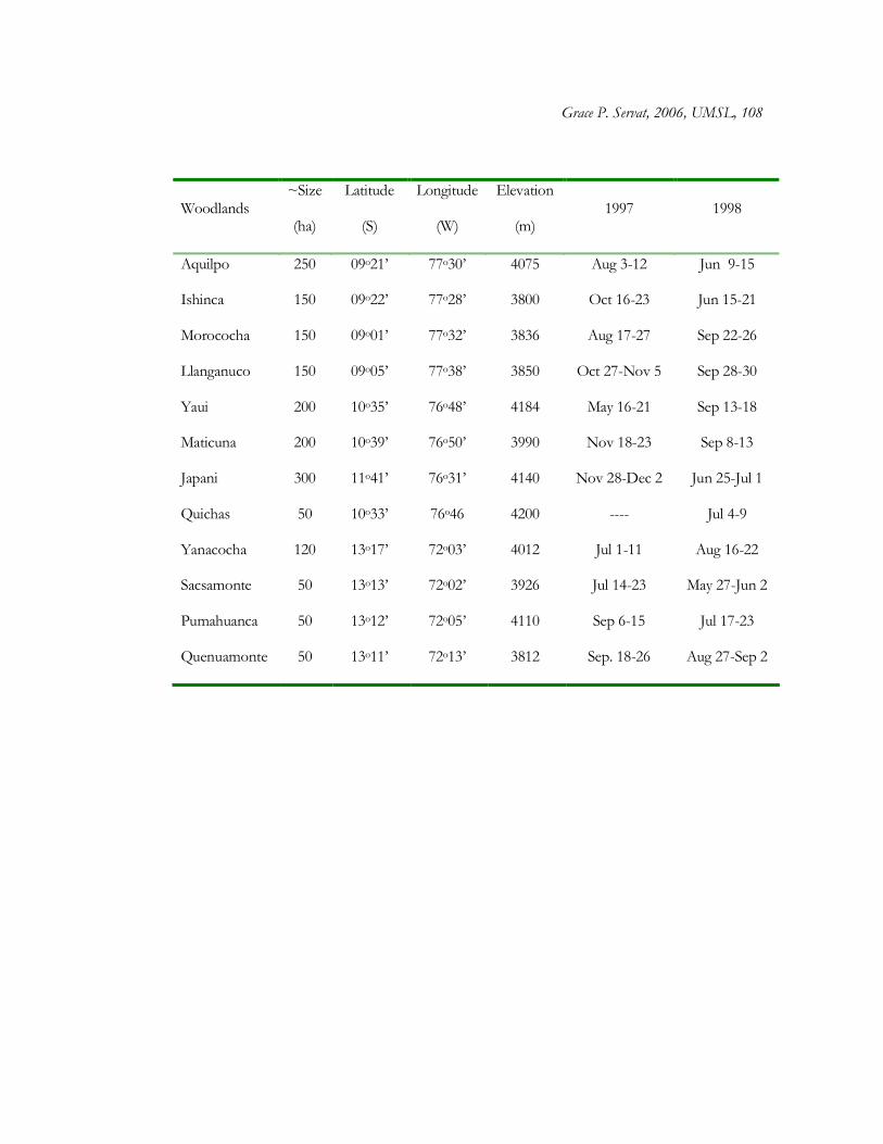
Grace P. Servat, 2006, UMSL, 108
Woodlands ~Size
(ha)
Latitude
(S)
Longitude
(W)
Elevation
(m) 1997 1998
Aquilpo 250 09o21’ 77o30’ 4075 Aug 3-12 Jun 9-15
Ishinca 150 09o22’ 77o28’ 3800 Oct 16-23 Jun 15-21
Morococha 150 09o01’ 77o32’ 3836 Aug 17-27 Sep 22-26
Llanganuco 150 09o05’ 77o38’ 3850 Oct 27-Nov 5 Sep 28-30
Yaui 200 10o35’ 76o48’ 4184 May 16-21 Sep 13-18
Maticuna 200 10o39’ 76o50’ 3990 Nov 18-23 Sep 8-13
Japani 300 11o41’ 76o31’ 4140 Nov 28-Dec 2 Jun 25-Jul 1
Quichas 50 10o33’ 76o46 4200 ---- Jul 4-9
Yanacocha 120 13o17’ 72o03’ 4012 Jul 1-11 Aug 16-22
Sacsamonte 50 13o13’ 72o02’ 3926 Jul 14-23 May 27-Jun 2
Pumahuanca 50 13o12’ 72o05’ 4110 Sep 6-15 Jul 17-23
Quenuamonte 50 13o11’ 72o13’ 3812 Sep. 18-26 Aug 27-Sep 2

Grace P. Servat, 2006, UMSL, 109
Table 2.2. Insectivorous species associated with Polylepis woodlands. The asterisk after the
species name indicates the bird species and subspecies included in the study. Polylepis
woodlands: AQ=Aquilpo, IS=Ishinca, MO=Morococha, LL=Llanganuco, UI=Yaui,
MA=Maticuna, JA=Japani, KI=Quichas, YA=Yanacocha, SA=Sacsamonte,
PU=Pumahuanca and QE=Quenuamonte. (1) Taxonomy follows Stotz et al. (1996); (2)
Abundance: C = common, species that throughout their range of distribution occur in
moderate to large numbers (densities of more than 5-6 individuals/ha) and are found easily
during brief periods of time (1-2 days). U = Uncommon, less numerous (densities of 2-4
individuals/ha) detected in proper habitat. R=rare, species scarce and seldom encounter
even during prolonged stays in the field. Many of these species are territorial or patchily
distributed and occur in small number (densities of 1-2/ha) throughout their range of
distribution; (3) Habitat: BU=bushes, FE=Polylepis forest edge, FI = Polylepis forest interior;
(4) Strata: U = understory, SC = sub-canopy, C = canopy, A = aerial.
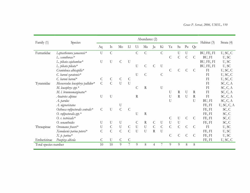
Grace P. Servat, 2006, UMSL, 110
Abundance (2) Family (1) Species
Aq Is Mo Ll Ui Ma Ja Ki Ya Sa Pu QeHabitat (3) Strata (4)
Furnariidae Leptasthenura yanacensis* U C C C C U U BU, FE, FI U, SC, C L. xenothorax* C C C C BU, FI U, SC L. pileata cajabambae* U U C U BU, FE, FI U, SC L. pileata pileata* U C C U BU, FE, FI U, SC Cranioleuca albicapilla* C C C C FI U, SC, C C. baroni zaratensis* U C C FI U, SC, C C. baroni baroni* C C C C FI U, SC, C Tyrannidae Mecocerculus leucophrys pallidior* C C U U FI SC, C, A M. leucophrys spp.* C R U FI SC, C, A M. l. brunneomarginatus* U R U R FI SC, C, A Anairetes alpinus U U R U R U R FI SC, C, A A. parulus U U BU, FI SC, C, A A. nigrocristatus U FE, FI U, SC, C, A Octhoeca rufipectoralis centralis* C U C C FE, FI SC, C O. rufipectoralis.spp.* U R FE, FI SC, C O. r. tectricialis* C U C C FE, FI SC, C O. oenanthoides U U U C R C U U U FE, FI SC, C Thraupinae Oreomanes fraseri* U C U C U U C C C C C C FI U, SC Xenodacnis parina petersi* C C C C U U R U FE, FI U, SC X. p. parina* C C C C FE, FI U, SC Emberizinae Poospiza alticola C U C C FE, FI U, SC, C Total species number 10 10 9 7 9 8 4 7 9 9 8 8

Grace P. Servat, 2006, UMSL, 111
Table 2.3. Inter and intraspecific variation in niche breadth of arboreal-insectivore birds
across forests nested within three regions. The niche breadth value of each individual bird
for each population was used as replicates in Hierarchical MANOVA tests (F). Asterisks (*)
indicate significance levels: * = P < 0.05, ** = P < 0.01, *** = P < 0.001 after Tukey Post
hoc test.
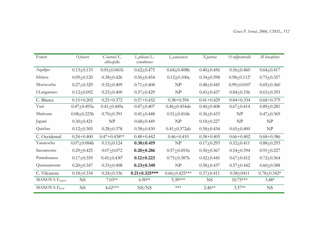
Grace P. Servat, 2006, UMSL, 112
Forest O.fraseri C.baroni/C.albicapilla
L.pileata/L. xenothorax
L.yanacensis X.parina O.rufipectoralis M leucophrys
Aquilpo 0.13+0.133 0.05+0.061b 0.62+0.475 0.64+0.408b 0.40+0.456 0.56+0.460 0.64+0.417 Ishinca 0.09+0.120 0.38+0.426 0.56+0.454 0.12+0.100a 0.34+0.398 0.98+0.112a 0.75+0.357 Morococha 0.27+0.329 0.32+0.409 0.71+0.408 NP 0.48+0.445 0.99+0.010b 0.69+0.360 LLanganuco 0.12+0.092 0.23+0.400 0.37+0.429 NP 0.43+0.437 0.84+0.336 0.63+0.393
C. Blanca 0.15+0.202 0.25+0.372 0.57+0.452 0.38+0.394 0.41+0.429 0.84+0.334 0.68+0.379 Yaui 0.47+0.493a 0.41+0.449a 0.47+0.407 0.46+0.454ab 0.40+0.408 0.67+0.414 0.89+0.281 Maticuna 0.08+0.223b 0.70+0.391 0.41+0.448 0.51+0.416b 0.36+0.433 NP 0.47+0.369 Japani 0.30+0.421 NP 0.68+0.449 NP 0.18+0.227 NP NPQuichas 0.12+0.305 0.28+0.378 0.38+0.430 0.41+0.372ab 0.58+0.434 0.65+0.400 NP
C. Occidental 0.24+0.400 0.47+0.438** 0.48+0.442 0.46+0.410 0.38+0.405 0.66+0.402 0.68+0.386 Yanacocha 0.07+0.084b 0.13+0.124 0.30+0.419 NP 0.17+0.293 0.52+0.411 0.88+0.293 Sacsamonte 0.29+0.425 0.07+0.072 0.20+0.286 0.57+0.451b 0.30+0.367 0.54+0.394 0.91+0.227 Pumahuanca 0.17+0.359 0.45+0.430b 0.12+0.223 0.75+0.387b 0.42+0.445 0.67+0.412 0.72+0.364 Quenuamonte 0.20+0.347 0.33+0.408 0.23+0.340 NP 0.58+0.437 0.57+0.442 0.60+0.388
C. Vilcanota 0.18+0.334 0.24+0.336 0.21+0.325*** 0.66+0.425*** 0.37+0.411 0.58+0411 0.78+0.342*MANOVA Fregion NS 7.03** 6.90** 5.39*** NS 10.75*** 3.48*MANOVA Flocal NS 4.62*** NS/NS *** 2.46** 3.37** NS

Grace P. Servat, 2006, UMSL, 113
Table 2.4. Foraging strategies of insectivorous birds. Data in the table includes foraging
niche breadth (Levin’s index) and plasticity results for each bird species based on the
statistical significance of hierarchical MANOVA tests (see text for calculations). (n) =
number of populations. Asterisks indicate significance levels: * = P < 0.05, ** = P < 0.01,
*** = P < 0.001 after Tukey Post hoc test..

Grace P. Servat, 2006, UMSL, 114
Niche breadth in microhabitat use
Niche plasticity in c value position
Bird Species
Niche range size
MANOVA F(local)
MANOVA F(local)
Foraging strategy
Oreomanes fraseri (n=12) 0.05-0.47 NS NS Specialist-restricted
Cranioleuca baroni/C albicapilla (n=12) 0.13-0.70 4.62** 3.05*** Generalist-plastic
Leptasthenura pileata (n=8) 0.37-0.71 * NS Generalist-restricted
L. xenothorax (n=4) 0.12-0.30 NS 4.17*** Specialist-plastic
L. yanacensis (n=7) 0.12-0.75 5.39** NS Generalist-restricted
Xenodacnis parina (n=12) 0.17-0.58 2.46* NS Generalist-restricted
Mecocerculus leucophrys (n=10) 0.47-0.91 NS 3.75** Generalist-plastic
Octhoeca rufipectoralis (n=10) 0.52-0.99 3.37 5.74*** Generalist-plastic

Grace P. Servat, 2006, UMSL, 115
Table 2.5. Food resources abundance (arthropods/microhabitat). Hierarchical MANOVA
results for arthropod abundance at each microhabitat across 12 woodlands and 3 regions of
study based on two replicate plots per forest. Significance of F-values for local and regional
effects is indicated as: ** = P < 0.01, ** = P < 0.001, NS = No significant differences.
Superscripts following means indicate differences across sites (a, b, c) or regions (A, B) after
post-hoc Tukey test. NP = not present.

Grace P. Servat, 2006, UMSL, 116
Arthropod abundance per microhabitat Forests and Regions
Polylepis foliage Polylepis bark Moss Gynoxys foliage Tristerix foliage
Aquilpo 41.0+11.3a 77.5+21.9a 139.0+11.3 25.0+0.0 5.5+4.9
Ishinca 58.5+0.7 76.0+22.6a 141.5+13.4 72.5+62.9 20.0+25.5
Morococha 69.0+32.5 134.0+8.5 65.5+4.9a 44.0+15.5 62.5+30.4
Llanganuco 57.0+26.8 89.0+11.3 50.0+12.7a 36.0+21.2 NP
C. Blanca 56.4+19.7B 119.0+59.2B 99.0+45.3A 44.4+31.9A 29.3+31.9
Yaui 70.5+10.6 144.5+40.3 84.0+8.5 11.0+0.0 68.0+65.1
Maticuna 120.5+2.1 231.5+44.5b 436.0+120.2b 75.0+72.1 30.0+16.9
Japani 244.5+7.8c 214.5+74.2 205.5+45.9 NP 47.0+63.6
Quichas 142.5+34.6b 109.5+0.70 83.5+34.6 158.5+37.1 47.5+31.8
C. Occidental 144.5+69.2A 175.0+64.4A 202.3+161.8B 81.5+75.4B 48.1+39.7
Yanacocha 61.5+3.5 108.0+41.0 256.5+60.1 88.5+41.7 NP
Sacsamonte 58.0+22.6 53.5+13.4 179.5+48.8 81.5+12.0 NP
Pumahuanca 129.0+12.7 71.5+9.2a 153+11.3 120+9.2 NP
Quenuamonte 53.0+9.9 119.5+28.9a 138.5+57.3 57+39.6 NP
C. Vilcanota 75.4+34.8B 88.1+34.8B 181.9+60.9B 86.9+33.1B NP
MANOVA Local F11,24
20.1*** 5.6** 9.6*** NS NS
MANOVA Region F2,10
*** 19.4*** 16.2*** 8.1** --

Grace P. Servat, 2006, UMSL, 117
Table 2.6. Floristic composition across Polylepis woodlands. Hierarchical MANOVA results
for plant species richness and abundance across regions and forests. Asterisks indicate levels
of significance: * = P < 0.05, ** = P < 0.01, *** = P < 0.001, NS = no significance.
Superscripts following means indicate differences across sites (a, b, c) or regions (A, B) after
Post hoc Tukey’s test.
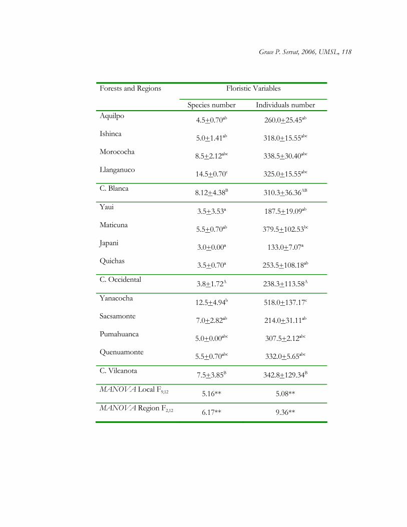
Grace P. Servat, 2006, UMSL, 118
Floristic Variables Forests and Regions
Species number Individuals number Aquilpo 4.5+0.70ªb 260.0+25.45ªb
Ishinca 5.0+1.41ªb 318.0+15.55ªbc
Morococha 8.5+2.12ªbc 338.5+30.40ªbc
Llanganuco 14.5+0.70c 325.0+15.55ªbc
C. Blanca 8.12+4.38B 310.3+36.36AB
Yaui 3.5+3.53ª 187.5+19.09ªb
Maticuna 5.5+0.70ªb 379.5+102.53bc
Japani 3.0+0.00ª 133.0+7.07ª
Quichas 3.5+0.70ª 253.5+108.18ªb
C. Occidental 3.8+1.72A 238.3+113.58A
Yanacocha 12.5+4.94b 518.0+137.17c
Sacsamonte 7.0+2.82ªb 214.0+31.11ªb
Pumahuanca 5.0+0.00ªbc 307.5+2.12ªbc
Quenuamonte 5.5+0.70ªbc 332.0+5.65ªbc
C. Vilcanota 7.5+3.85B 342.8+129.34B
MANOVA Local F9,12 5.16** 5.08**
MANOVA Region F2,12 6.17** 9.36**

Grace P. Servat, 2006, UMSL, 119
Table 2.7. Multivariate hierarchical ANOVA results for horizontal vegetation structure
variables. Means and SD are shown for all variables across 12 woodlands based on two
replicate plots. Significance of F-values for local and regional effects is indicated as * = P <
0.05, ** = P < 0.01, *** = P < 0.001. Superscripts following means indicate differences
across sites (a, b, c, d, e) or regions (A, B) according to Tukey multiple comparison among
means test. TBA = total basal area (800 m2), TD = tree density (# trees /800 m2), SD =
shrub density (# shrubs /800 m2), DBH 1 = number of individuals in size class 1 (> 10 – 20
cm dbh), DBH 2 = number of individuals in size class 2 (> 20 - 30 cm dbh), DBH 3 =
number of individuals in size class 3 (> 30 cm dbh). AC = absent category. NS = No
significant differences.

Grace P. Servat, 2006, UMSL, 120
Horizontal Vegetation Structure Variables Forests and Regions TBA TD SD DBH1 DBH2 DBH 3
Aquilpo 537.5 + 53.84b 104.5 + 12.02 165.0 + 0.00ab 40.5+4.90 15.5+2.12ab 0.5 +0.70b
Ishinca 340.3 + 61.85ab 91.0 + 19.79 269.0+11.51ab 56.6+12.02 31.5+7.77abc 3.0 +0.00b
Morococha 175.5 + 76.57a 70.5 + 34.64 268.5+45.96ab 54.0+31.11 16.0+2.82ab 0.5 +0.70b
Llanganuco 157.4 + 18.51a 56.5 + 6.36 264.5+2.12ab 56.6+13.43 39.5+2.12bc 8.5 +3.53a
C. Blanca 302.7 +169.31A 80.6+25.35AB 241.7+50.67AB 51.8+5.44 25.6+11.57A 3.1 +3.75
Yaui 363.7 +12.19ab 83.0 +2.82 101.0 +72.12a 45.5+7.77 33.5+6.36abc 4.30+1.51b
Maticuna 59.4 +42.09a 42.0 +24.04 273.0+47.07ab 40.5+23.33 1.5+0.70a AC
Japani 75.3 +10.75a 48.5 +3.53 32.5 +13.43a 46.0+2.82 2.5+0.70a AC
Quichas 131.0 +19.68a 65.5 +6.36 175.5+132.22ab 57.0+11.51 8.0+4.24ab 0.5 +0.70b
C. Occidental 157.3 +131.82B 59.7+19.52A 145.5+124.38A 47.2+12.13 11.5+14.21B 1.1 +1.88
Yanacocha 550.4 +213.66b 149.0+35.35 463.0 +79.60b 82.5+9.19 65.0+25.45c 1.5 +0.70b
Sacsamonte 350.6+106.08ab 56.0 +9.89 160.5+41.71ab 25.0+9.89 24.0+4.24ab 7.0 +4.24b
Pumahuanca 175.7 +15.43a 85.5 +14.84 189.0+80.61ab 72.5+20.50 12.0+4.24ab AC
Quenuamonte 370.0+162.58ab 101.5+51.61 251.5+27.57ab 67.5+44.54 26.5+9.19ab 4.0 + 4.24b
C. Vilcanota 361.7 +177.37A 98.0+43.58B 266.0+148.04B 61.8+30.34 31.8+23.70A 3.1 + 3.64
ANOVA Local F9,12 6.03** NS 2.90* NS 7.90*** 4.16*
ANOVA Region F2,12 10.73** 5.29* 4.43* NS 11.70** NS
MANOVA Local F9,12 = 3.33*
MANOVA Region F2,12 = NS

Grace P. Servat, 2006, UMSL, 121
Table 2.8. Hierarchical MANOVA results for vertical vegetation structure variables. Means
and SD are shown for all variables across 12 woodlands based on two replicate plots.
Significance of F-values for local and regional effects is indicated as: * = P < 0.05, ** = P <
0.01, *** = P < 0.001, NS = No significant differences. Superscripts following means
indicate differences across sites (a, b, c, d, e) or regions (A, B) according to Post-hoc
Tukey’s test. FHDEN1 = foliage height density or proportional coverage at > 0 – 2 m,
FHDEN2 = foliage height density at > 2 – 6 m, FHDEN3 = foliage height density at > 6 –
10 m, HEIGHT = mean tree height (m). ND = No data available.

Grace P. Servat, 2006, UMSL, 122
Vertical Vegetation Structure Variables Forests and Regions
FHDEN1 FHDEN2 FHDEN3 HEIGHT
Aquilpo 0.10 + 0.07a 0.17 + 0.02a 0.72 + 0.05de 12.9 + 2.55b
Ishinca 0.09 + 0.02a 0.10 + 0.09a 0.80 + 0.07e 7.6 + 0.11ab
Morococha 0.33 + 0.08ab 0.42 + 0.02abc 0.24 + 0.06abc 8.4 + 1.59ab
Llanganuco 0.34 + 0.01ab 0.47 + 0.09abc 0.18 + 0.08ab 4.4 + 1.56a
C. Blanca 0.21 + 0.13 0.29 + 0.17A 0.48 + 0.30A 8.3 + 3.48
Yaui 0.10 + 0.06a 0.29 + 0.01ab 0.60 + 0.04cde 7.6 + 0.36ab
Maticuna 0.56 + 0.16b 0.42 + 0.14abc 0.01 + 0.02a 4.5 + 2.88a
Japani 0.23 + 0.04a 0.71 + 0.02c 0.05 + 0.06a 7.3 + 3.69ab
Quichas 0.26 + 0.07ab 0.59 + 0.00bc 0.14 + 0.07ab 6.8 + 0.94ab
C. Occidental 0.28 + 0.19 0.50 + 0.18B 0.20 + 0.25B 6.6 + 2.22
Yanacocha 0.17 + 0.08a 0.26 + 0.12ab 0.56 + 0.20cde 7.9 + 1.24ab
Sacsamonte 0.16 + 0.08 0.34 + 0.22 0.50 + 0.14bcde 8.8 + 1.75ab
Pumahuanca 0.30 + 0.04ab 0.45 + 0.11abc 0.25 + 0.07abc 7.0 + 0.48ab
Quenuamonte 0.28 + 0.09ab 0.37 + 0.01abc 0.35 + 0.08abcd 7.4 + 0.53ab
C. Vilcanota 0.22 + 0.09 0.35 + 0.12A 0.41 + 0.16A 7.8 + 1.12
ANOVA Local F9,12 6.18** 4.84** 14.64*** 3.00*
ANOVA Region F2,12 NS 9.36*** 19.23*** NS
MANOVA Local F9,12 = 2.46**
MANOVA Region F2,12 = NS

Grace P. Servat, 2006, UMSL, 123
Table 2.9. Mantel tests using 999 permutations and the program Permute (Casgrain 1998).
Each line in the table is a model that examines the influence of region, floristic
compositions, vegetation structure, and arthropod abundance, on bird species foraging. n=
number of pair site combinations used in the model (see text for calculations). Partial
regression coefficients for each predictor variable and overall model R2 are provided.
Significance of models is indicated by: * = P < 0.05, ** = P < 0.01, *** = P < 0.001, NS =
No significant differences.

Grace P. Servat, 2006, UMSL, 124
Predictor Variables
Models Region Floristic
compositionHorizontal structure
Vertical structure
Arthropod abundance
Overall R2
Oreomanes fraseri (n=66) 0.034 0.087 -0.108 0.060 0.162 NS
Cranioleuca baroni/albicapilla (n=44/22) 0.160
-0.022 0.087 0.067 0.385*** 0.15**
Leptasthenura pileata xenothorax (n=44/22) -0.047 -0.030 -0.186 0.316** 0.114** 0.10**
Leptasthenura yanacensis (n=21) 0.114 0.112 -0.494* -0.280 -0.089 0.24*
Xenodacnis parina (n=55) 0.203* 0.259** -0.119 0.020 0.258** 0.15**
Mecocerculus leucophrys (n=45) -0.246* -0.005 -0.186 -0.066 0.468** 0.30**
Octhoeca rufipectoralis (n=45) -0.050 -0.196 -0.110 0.179 0.406** 0.16**

Grace P. Servat, 2006, UMSL, 125
CHAPTER THREE
BIRD ASSEMBLAGE STRUCTURE IN THE POLYLEPIS COMMUNITY
Much of the past four decades of community ecology have been devoted to the
analyses of community structure and organization (Diamond 1975, Connor and Simberloff
1979, Tilman 1982, 1988, Wiens 1986, 1989, Ricklefs 1987, Drake 1990, Cornell and Lawton
1992, Ricklefs and Schluter 1993, Losos 1994, 1998, Brown 1995, Huston 1999, Hubbell
2001, Leibold and Chase 2003). Yet, questions regarding whether communities are assembled
randomly or by repeatable processes, how local conditions and regional contingency influence
community organization, and the extent to which patterns of functional organization are
repeated in space and time, have remained poorly resolved issues (Ricklefs and Schluter 1993,
Brown 1995, Huston 1999, Hubbell 2001, Leibold and Chase 2003).
Our perceptions of community organization are influenced by a historical dichotomy
of “individualistic” versus “organismal” classifications. Clements (1916) compared the plant
community to an organism, ‘‘able to essentially reproduce its component parts’’, whereas
Gleason (1926) argued that a plant community is “scarcely even a vegetation unit, but merely
a coincidence of the range of species”. Presently, the individualistic-organismal debate has
been invigorated by the “neutral” and “niche” based models of community ecology. Neutral
models (Hubbell 2001) view all species as equal or functionally equivalent, so they exert
similar effects both on populations and on community organization. In contrast, niche-based

Grace P. Servat, 2006, UMSL, 126
models grant species particular properties, and thus, recognize species as functionally distinct,
with unique or non-substitutable roles (Chave et al. 2002, Chase and Leibold 2003).
Regardless of the debate over its nature, the complexity of natural communities
makes it unlikely they function only as either groups of individual species present because of
individual tolerances, or as assemblages of perfectly integrated species (Ricklefs 1987, Ricklefs
and Schluter 1993, Ricklefs 2001). Instead, communities are regarded as a template from
which a large number of local (e.g., past and present ecological processes), and/or historical
factors (i.e., those that shaped the community from its beginning such as dispersal, speciation,
migration, and extinction), which operate at different spatial and temporal scales, convene to
shape particular aspects of their structure and organization (Vuilleumier and Simberloff 1980,
Wiens 1986, 1989, Ricklefs 1987, Ricklefs and Schluter 1993, Losos 1994, 1998, Brown 1995,
Huston 1999, Ricklefs 2001).
Analyses of community structure are conventionally made by breaking down groups
of species (not necessarily related taxonomically) into “functional groups” or “guilds” (Root
1967), with the underlying assumption that the relationship between species and function is
intimately linked (i.e., species with similar ecological attributes seem to act or respond to
environmental variation in similar ways) (Walker 1992, Lawton and Brown 1994, see review in
Chase and Leibold 2003). Although, guilds are considered to be “identifiable” and “constant”
within a community, guilds are not static in space and time and, it is precisely their dynamic
nature that makes them relevant to understand community structure (e.g., McNaughton 1978,
Cornell y Kahn 1989, Mac Nally 1994) and organization (e.g., Jaksic and Delibes 1987, Jaksic
and Medel 1990, Jaksic et al. 1993, Marti et al. 1993). A wide variety of criteria and levels of
subdivision have been used to make assignments of species into guilds to describe community

Grace P. Servat, 2006, UMSL, 127
structure (Karr 1971, 1976, 1980, Terborgh 1986, Szaro and Balda 1979, Blake 1983, Bradley
and Bradley 1983, Manuwal 1983, Recher and Holmes 1985). However, given that energy
acquisition is paramount to species survival and fitness, foraging ecology has been the
prevalent way to group species into guilds (e.g., Root 1967, Morse 1971, Holmes et al. 1979,
Sherry 1979, 1982, Holmes and Recher 1986, Landres and MacMahon 1983, Wiens 1983,
Brown 1989, Mac Nally 1994).
Fluctuation in abiotic (e.g., temperature, wind, Cody 1985, Wiens 1989) and biotic
factors, such as vegetation structure (e.g., vertical zonation of vegetation; MacArthur and
MacArthur 1961, MacArthur et al. 1962, Robinson and Holmes 1984, McNally 1994, Huston
1994), floristic composition (e.g., the richness and relative number of floristic elements;
Orians 1969, Recher 1969, James and Wamer 1982, Rotenberry 1985, Whitmore 1975, James
et al. 1984, Tomoff 1974), available food resources (Morse 1977, Jaksic 1981, Wiens 1983,
1989, Bradley and Bradley 1985) and species interactions (e.g., Connell 1983, Schoener 1983)
through its effects on foraging ecology of species, likely influence community structure (e.g.,
modifying species composition and/or abundance within guilds).
Studies that describe the extent of spatial variation in the structure of communities
and the factors in which the community is embedded are insightful, yet scarce (e.g.,
Vuilleumier and Simberloff 1980, Recher and Holmes 1985, Holmes 1986, Wiens 1989). In
this study, I examined the extent of spatial variation of an assemblage of forest-interior
insectivorous birds associated with the Polylepis community, a unique vegetation association of
the high Andes, using the conventional guild approach (i.e., guild classification, number of
guilds, and component bird species diversity and abundance). I describe variation in bird
species composition and abundance for each foraging guild across twelve Polylepis woodlands

Grace P. Servat, 2006, UMSL, 128
distributed along 600 km in the Peruvian Andes in light of variation of food resources
(available arthropods) and biological interactions (i.e., potential competition). I chose
availability in food resources because birds in Polylepis woodlands depend on arthropods for
foraging and thus fluctuations in availability of food resources could be a limiting factor. I
considered arthropods to be limited due to the low temperature, high radiation, dryness, and
other environmental variables characteristic of high elevation forests. I assess the relative
importance of resource availability in assemblage structure by measuring arthropod
abundance in microhabitats where birds’ forage (arthropods seem to be attached to protected
microhabitats such as the layers of bark) and its relationship with bird species composition
and abundance within and across guilds.
Bird species in the Polylepis system co-occur with different sets of species within its
range of distribution, in particular among regions of study. As species composition changes,
so too does the precise nature of species interactions (MacArthur and Wilson 1967, Whittaker
1972). Studies on several taxa have shown that competitive interactions can alter community
structure (e.g., rodents, Luo and Fox 1995; Orthoptera, Beckerman 2000; ants, Holldobler
and Wilson 1990). The outcome of “natural experiments” has been largely debated (Connor
and Simberloff 1979, Diamond and Gilpin 1982), but has lead to the search of other analytical
procedures such as null model tests (Gotelli 2000, Gotelli and Entsminger 2001). I compared
the niche overlap of observed and randomly generated assemblages using null models to
determine if structural patterns are consistent with competition theory (Gotelli and Graves
2003).
Although, competition and food resources available are not mutually exclusive factors
(Martin 1985, Kotler and Holt 1989), I hypothesize that availability of food resources is of

Grace P. Servat, 2006, UMSL, 129
primary importance to determine bird assemblage structure in the Polylepis system (“food
resources-hypothesis”). I expect that a) bird species richness and abundance within guilds will
follow the patterns of abundance in food resources within microhabitats across Polylepis
woodlands, and b) that niche overlap in the bird assemblage will be significantly larger than
expected by chance. However, if bird species richness and abundance within guilds follow the
patterns of abundance in food resources, and niche overlap in the bird assemblage is
significantly lower than expected by chance, I will interpret it as the result of present
interspecific competition (i.e., species in the assemblage are segregating due to competitive
exclusion)(“competition-hypothesis”). In addition if bird species richness and abundance
within guilds do not follow the patterns of abundance in food resources and niche overlap in
the assemblage is higher than expected by chance, could be interpreted as assemblage
instability (i.e., no competitive exclusion is present where it is expected to occur), or that other
factors, not assessed in the study, are more important in structuring the bird assemblage.
METHODS
The study system
Throughout the Peruvian Andes above 3500 m elevation, scattered Polylepis
woodlands are typically found close to streams or forming small patches in gorges on slopes
and cliff-edges, where they are surrounded by grasslands. The Polylepis community (defined
here as the group of organisms with broad taxonomic affinities that occur together and
interact within a framework of horizontal and vertical linkages, Giller and Gee 1987) is a
distinctive biological system characterized by high levels of endemism (Fjeldså and Krabbe

Grace P. Servat, 2006, UMSL, 130
1990, Fjeldså 1992a, b, c, 1993). The scattered distribution of Polylepis woodlands throughout
the Andes provides discrete units of study. For this study I selected four Polylepis woodlands
(> 50 ha) above 3500 m within each of three regions of the Peruvian Andes: Cordillera
Blanca, C. Occidental, and C. Vilcanota (see Chapter I and II for description). From north to
south the 12 sites selected for the present study and the dominant Polylepis tree species
occurring at each woodland were: 1) C. Blanca: Aquilpo and Ishinca (P. weberbauerii),
Morococha and Llanganuco (P. sericea); 2) C. Occidental: Yaui and Quichas (P. weberbauerii),
Maticuna and Japani (P. incana); and 3) C. Vilcanota: Yanacocha, Sacsamonte, Pumahuanca,
and Quenuamonte (P. racemosa). In each forest, I obtained data (i.e., bird species diversity and
abundance; food resource abundance) in two replicate sets of four 100 x 10 m transects
placed 50 m apart from each other. The last transect from the first set was separated by at
least 500 m from the first transect of the second set (see study design in Chapter II).
The bird assemblage
In the Andes of Peru approximately 35-40 bird species are found associated with the
Polylepis community. The avian assemblage in this community is composed approximately of
28 % frugivorous (species that mainly consume fruit, seeds, and flowers), 20 % nectarivorous
(species that mainly consume nectar), 2 % carnivorous (species that mainly consume
vertebrates), and 50 % insectivorous (species that mainly consume insects and other
arthropods) bird species (Fjeldså 1992, Fjeldså and Krabbe 1990, Fjeldså 1993, Herzog 2003).
I included forest interior insectivorous species as representatives of the avian assemblage
because they constitute ca. 80 % of the species that regularly breed and winter in Polylepis
woodlands (“core species”, Remsen 1994). In addition, insectivorous birds associated with the

Grace P. Servat, 2006, UMSL, 131
Polylepis community seem to be “stable” in terms of richness and abundance across seasons
when compared to frugivorous or nectarivorous (Herzog 2003) As some of the species in the
assemblage migrate or have very low occurrences, gathering enough foraging information on
all species is not possible and, therefore, I restricted the analyses to 10 core species: Oreomanes
fraseri, Cranioleuca baroni (replaced in the south by C. albicapilla), Leptasthenura pileata (replaced in
the south by L. xenothorax), L. yanacensis, Xenodacnis parina, Anairetes alpinus, A. nigrocristatus
(clustered together with A. parulus because of few observations for both), Mecocerculus
leucophrys, Octhoeca rufipectoralis, and O. oenanthoides.
Foraging observations.- I made observations of actively foraging birds at each Polylepis
forest throughout the day using focal animal sampling (Altman 1974) on core species. I
systematically covered transects and moved from one foraging bird to another. I obtained
observations from 10 individuals/species for each Polylepis forest. Continuous observations
were divided into 60-second sequences, in which I tallied the number of microhabitats (e.g.,
Polylepis bark or foliage) and maneuvers (e.g., glean, probe) used by each bird. I used the
foraging repertoire (25 categories from core-species) in Bray Curtis ordination (PC-ORD
Version 4, McCune and Mefford 1999) and selected Sorensen’s percent dissimilarity as a
measure of distance between points (individual birds), variance regression for end point
selection, and Euclidean distance for axis projection geometry (Beals 1984, Greig-Smith 1983,
McCune and Mefford 1999). In all cases, individual observations falling closer together in the
ordination were assumed to belong to the same foraging group. I nominated groups based on
the main foraging category used (e.g., foliage gleaners, bark gleaners). At each Polylepis forest, I
tested for differences among foraging groups using hierarchical Multivariate Analyses of
Variance (SPSS Release 12.0) using the scores along the first two ordination axes of all

Grace P. Servat, 2006, UMSL, 132
individuals by species as indicators of the gradient in ‘spatial variation’ where the species
occur. For each axis, species were nested within nominated guilds (using individuals as
replicates) and guilds nested within forest. When individuals of the same species fell into two
different groups, I used majority rules to decide guild membership (e.g., Holmes et al. 1979,
Landres and MacMahon 1980, 1983, Sabo 1980, Sabo and Holmes 1983). The analysis was
followed by post-hoc Tukey test (SPSS Release 12.0) to determine if species assigned to
groups were more similar in foraging categories used (i.e., not significantly different at
P<0.01) than species assign to different groups in all Polylepis woodlands.
Assemblage structure
I measured two components of assemblage structure, diversity and abundance of
birds within and across foraging guilds. I conducted bird censuses between 0600 and 0800 hrs
and 1500 to 1700 hrs, for four consecutive days in 1997 and six days in 1998. Censuses were
made by walking transects at a steady pace (ca. 1 km/hr) recording all birds heard and seen
(cf. Blake et al. 1994), supplemented by casual observations. I counted the total number of
species (i.e., richness) and the number of individuals per species (i.e., abundance), and
calculated bird species diversity across woodlands using rarefaction curves (Hurlbert 1971,
Sanders 1968) in the Program EcoSim 7.72 (Gotelli and Entsminger 1997-2005) to control
for differences in bird abundance while comparing richness across sites. The process was
simulated 1000 times specifying the number of individuals that are randomly drawn from
each sample. I compared the diversity across Polylepis woodlands using the same abundance
level (30 individuals) in all cases. I tested for significant differences in total bird abundance

Grace P. Servat, 2006, UMSL, 133
among and within guilds across Polylepis woodlands, using hierarchical MANOVA, followed
by Tukey’s test for post-hoc comparisons.
The potential role of food resource abundance and competition
Food resources.- I measured food resources available to birds by counting arthropods in
samples taken from five discrete microhabitats where birds were observed to forage: Polylepis
bark; Polylepis, Gynoxys, and Tristerix foliage; and moss (see design in Chapter II). I excluded
arthropods with less than 2 mm length, individuals with aposematic coloration, or taxa with
low occurrence (< 5 individuals per microhabitat), as they are unlikely to be prey for foraging
birds due to low acceptability or detectability (Wolda 1990, Servat 1995). I analyzed data on
arthropod abundance using hierarchical MANOVA (SPSS Release 12.0) followed by Tukey’s
to test for differences in arthropod abundance within microhabitats, and microhabitats within
Polylepis woodlands.
Competition.- To assess the role that competition may be playing in the system, I
compared the observed niche overlap of bird species in the assemblage with those generated
from null models using Pianka’s Index in the EcoSim Program Version 7.72 (Gotelli and
Entsminger 1997-2005). Comparisons of observed and randomly generated niche overlaps in
assemblages reveal if structural patterns are consistent with competition theory. If observed
patterns were not different from randomly generated communities then it will indicate no
evidence for competition. However, if different and in the predicted direction (less overlap
than expected), this will indicate consistency with competition theory. To construct the null
model, I made a matrix of all potential competitor species (i.e., all species that belonged to the
same guilds) (rows) by forest (columns). Cell values within each row of the observed matrix

Grace P. Servat, 2006, UMSL, 134
were reassigned without replacement, and mean niche overlap, which is based on
comparisons of all possible species pairs, was calculated during each run using RA3 algorithm
(Gotelli and Graves 1996). The RA3 algorithm takes into account observed values (e.g.,
proportional use of microhabitats) and because values are randomly reassigned to different
categories by rows, the rows of the utilization matrix are simply reshuffled, and the null model
effectively retains observed niche breadth values for each species (Gotelli and Graves 1996).
This procedure was repeated 1000 times to provide an overall mean and standard deviation of
niche overlap values that could be compared to observed values.
To determine if patterns of bird diversity and abundance within guilds across
woodlands was related to variation in food resources, I used Mantel test (PCORD Version
4.10, 1995-1999). For the models, I built pair wise-site distance matrices based on bird
diversity and abundance within guilds (response variable) at each forest, and food resource
abundance in microhabitats (predictor variable) to evaluate the null hypothesis of no
relationship in distance matrices. I used Sorensen’s dissimilarity index as a distance measure
and performed 999 permutations of the original matrix to determine the significance
probability of the observed relationship between the response and predictor variables.
RESULTS
Assemblage structure
Forest-independent ordinations of bird species in the assemblage (based on
similarities in foraging categories used by individuals) revealed three to four foraging groups
across Polylepis woodlands (Fig. 3.1). Overall, the farthest points along the first axis of the

Grace P. Servat, 2006, UMSL, 135
ordination separated individuals that glean or probe proportionally more in Polylepis bark,
from those that glean proportionally more in Polylepis or Gynoxys foliage (Fig. 3.1, Appendix
3.1). In the second axis the farthest points separated individuals that capture prey “in the air”
(i.e., hawking, hovering, or sally-gleaning) from foliage and bark foragers (Fig. 3.1, Appendix
3.1). Based on the general patterns just described, I named guilds as: “Polylepis bark foragers”,
mostly conformed by individuals of Oreomanes fraseri and Cranioleuca baroni/C. albicapilla, the
“foliage foragers” that included most individuals of Leptasthenura pileata/L. xenothorax, L.
yanacensis, and Xenodacnis parina, the “aerial hawkers” included most individuals of Mecocerculus
leucophrys, Anairetes alpinus, A. parulus/A. nigrocristatus (usually found in the canopy); and the
“aerial sit and sally gleaners” composed by most individuals of Octhoeca rufipectoralis and O.
oenanthoides (both of which are usually found in the understory).
Foraging position of individuals (along the two axes of the ordination) within same
guild was not significant different (P > 0.05) across Polylepis woodlands. However, when
comparing different guilds at each site, significant differences were detected in all Polylepis
woodlands as revealed by hierarchical MANOVA tests (Table 3.2), revealing groups of
species that differed in the use of the “foraging space”. Moreover, after post-hoc tests, I
found that individuals of some species were consistently attached to a particular foraging guild
(e.g., O. fraseri), while others were highly variable (e.g., X. parina and C. baroni/albicapilla) (Table
3.2). The inconsistency of some species across forests may result in some of the within-guild
variance found across Polylepis woodlands (Table 3.2).
Grace P. Servat, 2006, UMSL, 136
Diversity and abundance of insectivorous birds
Overall diversity of insectivorous bird species varied across Polylepis woodlands, as
revealed by rarefaction curves (Fig. 3.2). When number of individuals is controlled for (i.e., 50
individuals in Fig. 3.2) diversity was substantially higher in Aquilpo, Ishinca (C. Blanca),
Yanacocha, Sacsamonte and Pumahuanca (C. Vilcanota). On the other side, diversity was
lower in Japani, Quichas (C. Occidental), and Quenuamonte (C. Vilcanota) (Fig. 3.2),
suggesting that diversity of birds associated with the Polylepis system varies regionally.
Bird abundance (number of individuals/guild) among guilds was significantly
different in all Polylepis woodlands (MANOVA F3, 128 = 23.93, P < 0.001). Nonetheless, when
abundance of birds within same guilds was compared across woodlands, no differences were
found in bark foragers (F11,12 = 1.24, P = 0.356), foliage foragers (F16,19 = 0.91, P = 0.570),
hawkers (F6, 41 = 1.19 P = 0.326), or salliers (F8,15 = 2.07, P = 0.106) (Fig. 3.4).
The relative importance of competitive interactions and food resources in assemblage structure
Assemblages did not seem to be structured by competition, as revealed by null models
of niche overlap. In all models I found higher foraging overlap than expected by chance,
significantly so in 6 forests (Table 3.4), a predicted result for assemblages not structured by
competition.
Food resources abundance (arthropods) differed significantly across Polylepis
woodlands within and among microhabitats. I found significant differences in arthropod
abundance in moss (ANOVA F11,12 = 9.58, P < 0.0001), Polylepis bark (ANOVA F11,12 = 5.64,
P = 0.003), Polylepis foliage (ANOVA F11,12 = 20.11, P < 0.0001), and Gynoxys foliage

Grace P. Servat, 2006, UMSL, 137
(ANOVA F10,11 = 2.73, P = 0.05) across sites, but not in Tristerix foliage (P = 0.69). Basically,
moss, Polylepis bark, and Polylepis foliage contributed most to these differences.
The relative importance of food resources in bird species richness and abundance
assessed by Mantel tests; shows a direct and positive relationship between pair-wise site
similarities in abundance and richness of birds in the assemblage and pair-wise site similarities
in food resources (r2 = 0.43 and r2 = 0.33 respectively, P < 0.001, n = 66 pairs), which
supports predictions of the “local food resources hypothesis”.
DISCUSSION
Foraging guilds identities (i.e., Polylepis bark foragers, foliage foragers, aerial foragers)
were present and largely consistent in most Polylepis woodlands. However, bird species
identities and its abundance at each guild were not necessarily similar across forests, which
may be due in part to regional differences in insectivorous bird species diversity and
intrapopulation variation in foraging ecology (Chapter II).
High overlap among species in the avian assemblage across Polylepis woodlands
suggests that competitive interactions do not support the classic scenario expected by
competition theory (Hutchinson 1957, MacArthur and MacArthur 1961, Urban and Smith
1989), a result supported by several studies based on field observations or assessed through
null models in other communities (e.g., Inger and Colwell 1977, Vitt and Caldwell 1994, Vitt
and Zani 1998, 1996). The considerable overlap found in bird assemblages of Polylepis
woodlands, suggests that species may be able to coexist through other mechanisms (e.g.,
microhabitat or prey differentiation) (Hofer et al. 2000). Nonetheless, in the present study

Grace P. Servat, 2006, UMSL, 138
some aspects of competition may have not been detected (e.g., diffuse competition,
interference competition).
The role of food resource abundance in bird assemblage structure
Site similarities in species abundance across woodlands were related to site similarities
in food resources available, suggesting that birds are able to “track” food resources, or that
bird species converge in using food resources in the only microhabitats available (Pianka
1980, Jaksic 1981, Wiens 1983, 1989, Bradley y Bradley 1985).
Abundance and predictable resources may play a major role in structuring the
assemblage of birds associated with the Polylepis community. Some foraging microhabitats
were more predictable (e.g., Polylepis bark and foliage) than others (e.g., Tristerix or Gynoxys
foliage), so bird species adapted to exploit resources in unpredictable microhabitats were
absent (C. baroni in Japani) or switch microhabitats (e.g., X. parina). However, without
complementary experimental manipulations, the relative role of food resources (and
competition) influencing present-day community structure can not be unambiguously
determined.
Present distribution of Polylepis woodlands (e.g., isolation and habitat extent) suggests
an important role for history as a determinant of present day assemblage structure (e.g.,
Askins et al. 1987, Balent and Courtiade 1992, Lescourret and Genard 1994, Daniels et al.
1992). One of the major determinants of change in recent earth history was cyclic changes in
climate and topography during the Pleistocene (Shackleton et al. 1990, and Hooghiemstra and
Ran 1994). Many Cordilleras in Peru were covered by ice repeatedly over the last 2-3 million
years, which may have restricted species to lower elevations on the Andean slopes, and to

Grace P. Servat, 2006, UMSL, 139
certain mountain basins that remained ice-free (Simpson 1975, Simpson and Todzia 1990,
Fjeldså and Kessler 1996). The iced-covered mountain caps may have isolated some refuges
with Polylepis woodlands from the continuous band of humid shrubbery that is thought to
have remained along the Andes. Isolation during glaciations may have promoted species
differentiation, remaining endemic to their area of origin (Fjeldså and Kessler 1996). These
relict populations that survived periods of global climatic change likely were the source pool
of species for colonization of other areas as the glaciers receded (Simpson and Todzia 1990,
Fjeldså et al. 1999). In addition, Polylepis woodlands disrupted by tectonics and erosion may
have become isolated by barriers (e.g., Apurímac Canyon). Dispersal during interglacial
periods and post-glacial periods could have been an important influence in explaining present
bird composition patterns (Simpson 1975, Fjeldså and Kessler 1996).
Ecological research traditionally has focused on intra-community patterns, especially
on the role of competition and other species interactions in community structure (Symstad et
al. 2000; Caddle and Greene 1993; Cornell and Lawton 1992; Latham and Ricklefs 1993;
Francis and Currie 1998; Huston 1999); and few systematic, quantitative, spatial scale
descriptions have been done Descriptive studies on a large spatial scale, acknowledge the
complexity of communities as a dynamic collection of species integrated to varying degrees by
numerous factors (ecological and historical) and highlight the likely factors that generate
patterns and the scale at which future field studies should be conducted.
This study highlights the importance of considering the spatial scale in the
interpretation of patterns of assemblage structure (Levin 1992). In the Polylepis community,
bird assemblages at local scales appear non-random, with birds separating into distinct guilds.
However, at larger scales one sees that the identities and species richness, but not abundance

Grace P. Servat, 2006, UMSL, 140
in guilds vary. Conclusions derived from one or a few sites in this system would likely fail to
unravel the relative importance that local factors play in assemblage structure in the Polylepis
system. Moreover, incorporating the spatial variation in guild composition to assess
similarities in functioning is of great importance, because any relationship between diversity
and community processes may be driven by functional redundancy or by diversity of species
having different functional roles.
REFERENCES
Altmann, J. 1974. Observational study of behavior: sampling methods. Behaviour 49:227-267.
Askins, R. A., M. J. Philbrick, and D. S. Sugeno. 1987. Relationship between the regional
abundance of forest and the composition of forest bird communities. Biological Conservation 39:129-152.
Balent, G., and B. Courtiade. 1992. Modeling bird communities/landscape patterns
relationships in a rural area of south-western France. Landscape Ecology 6:195-211. Beals, E. W. 1984. Bray-Curtis ordination: an effective strategy for analysis of multivariate
ecological data. Advances in Ecological Research 14:1-55. Beckerman, B. A. 2000. Counterintuitive Outcomes of Interspecific Competition between
Two Grasshopper Species along a Resource Gradient. Ecology, Vol. 81, No. 4, pp. 948-957
Blake, J. G. 1982. Influence of fire and logging on nonbreeding bird communities of ponderosa pine forests. J. Wildl. Manage. 46:404-415.
Blake, J. G., J. M. Hanowski, G. J. Niemi, P. T. Collins. 1994. Annual Variation in Bird
Populations of Mixed Conifer-Northern Hardwood Forests. Condor, Vol. 96, No. 2, pp. 381-399
Bradley, R.A., and D.W. Bradley. 1993. Wintering shorebirds increase after kelp (Macrocystis) recovery. Condor 95:372-376.
Brown, J. S. 1989. The role of resource variability in structuring desert rodent communities.
Pp. 141-154 en Morris, D. W., Z. Abramsky, B. J. Fox & M. R. Willig (Eds.) Patterns

Grace P. Servat, 2006, UMSL, 141
in the structure of mammalian communities. Texas Tech University Press, Lubbock, Texas. 266 pp.
Brown, J. H. 1995. Macroecology. University of Chicago Press, Chicago. Cadle, J.E. and H.W. Greene. 1993. Phylogenetic patterns, biogeography, and the ecological
structure of neo-tropical snake assemblages. Pages 281-293 in R.E. Ricklefs and D. Schluter, editors. Species diversity in ecological communities: historical and geographic perspectives. University of Chicago Press, Chicago, Illinois, USA.
Casgrain, P. 1998. Permute! Université de Montréal, Montréal. Chase, J. M. and M. A. Leibold. Ecological Niches: Linking Classical and Contemporary
Approaches. 221 pp. Chave, J., H. C. Muller-Landau, and S. A., Levin. 2002. Comparing classical community
models: theoretical consequences for patterns of diversity. Am. Nat. 159, 1-23. Clements, F. E. 1916. Plant succession: an analysis of the development of vegetation.
Publication 242. Carnegie Institute, Washington, D.C. Cody, M. L. 1999. Assembly rules in plant and bird communities. Cambridge Univ. Press. Connell, J. H. 1983. On the prevalence and relative importance of interspecific competition:
evidence from field experiments. American Naturalist 122: 661-696 Connor, E. F. and Simberloff, D. 1979. The assembly of species communities: chance or
competition? Ecology, 60, 1132-40. Cornell, H. V. J. H. Lawton. 1992. Species interactions, local and regional processes, and
limits to the richness of ecological communities: a theoretical perspective. . Journal of Animal Ecology 61:1-12.
Cornell, H. V., and D. M. Kahn. 1989. Guild Structure in the British Arboreal Arthropods -
Is It Stable and Predictable. Journal of Animal Ecology, 58:1003-1020. Daniels, R. J. R., N. V. Joshi, and M. Gadgil. 1992. On the relationship between bird and
woody plant species diversity in Uttara Kannada district of South India. Proceedings of the National Academy of Sciences (USA) 89:5311–5315.
Diamond, J. M. 1975. Assembly of Species Communities, in Ecology and Evolution of
Communities (eds. M.L. Cody and J.M. Diamond), Belknap, Harvard, pp. 342-444. Drake, J. A. 1990. Communities as assembled structures: Do rules govern pattern? Trends in Ecology & Evolution Vol. 5, no. 5, pp. 159-164. 1990.

Grace P. Servat, 2006, UMSL, 142
Diamond, J. M. & M. E. Gilpin. 1982. Examination of the "null" model of Connor and Simberloff for species cooccurrences on islands. Oecologia 52: 64-74.
Fjeldså, J. 1992a. Biogeography of the birds of the Polylepis woodlands of the Andes. Paramo. Fjeldså, J. 1992b. Biogeographic patterns and evolution of the avifauna of relict high
altitude woodlands of the Andes. Steenstrupia 18:9-62. Fjeldså, J. 1992c. Un análisis biogeográfico de la avifauna de los bosques de quenoa (Polylepis)
de los Andes y su relevancia para establecer prioridades de conservación. Memorias del Museo de Historia Natural 21: 207-221.
Fjeldså, J. 1993. The avifauna of the Polylepis woodlands of the Andean highlands: the
efficiency of basing conservation priorities on patterns of endemism. . Bird Conservation International 3:37-55.
Fjeldså, J., and M. Kessler. 1996. Conserving the biological diversity of Polylepis woodlands of
the highlands of Peru and Bolivia. A contribution to sustainable natural resource management in the Andes. NORDECO, Copenhagen, Denmark.
Fjeldså, J. and N. Krabbe. 1990. Birds of the high Andes. Copenhagen and Apollo books.
Svendborg. Fjeldså, J. et al. 1999. Correlation between endemism and local ecoclimatic stability
documented by comparing Andean bird distributions and remotely sensed land surface data. Ecography 22:63-78.
Francis, A. P. and D. J. Currie. 1998. Global patterns of tree species richness in moist
forests: another look. Oikos 81:598-602. Giller, P. S. and J. H. R. Gee. 1987. The analysis of community organization: the influence
of equilibrium, scale and terminology. Blackwell Scientific Publications, Oxford, England.
Gleason, H. A. 1926. The individualistic concept of the plant association. Bulletin of the
Torrey Botanical Club 53:1-20. Gotelli, N. J. and G. L. Entsminger. 2000 EcoSim: Null models software for ecology.
Version 5.0. Acquired Intelligence Inc. & Kesey-Bear. Gotelli, N. J. and G. Graves. 1996. Null Models in Ecology. Smithsonian Institution Press,
Washington DC. Graves, G. R. and N. G. Gotelli. 1993. Assembly of avian mixed-species flocks in
Amazonia. Proceedings of the National Academy of Sciences USA 90:1388-1391.

Grace P. Servat, 2006, UMSL, 143
Herzog, S. K., Soria R., and E. Matthysen. 2003. Seasonal variation in avian community composition in a high-andean Polylepis (Rosaceae) forest fragment. The Wilson Bulletin: 115, p. 438-447.
Hooghiemstra, H. Ran, E. T. H. 1994. Late Phocene-Pleistocene High Resolution Pollen
Sequence of Colombia: An Overview of Climatic Change. Quaternary International: Vol 21, Pp. 63.
Hofer, U., H. Baur, and L. F. Bersier. 2003. Ecology of Three Sympatric Species of the
Genus Chamaeleo in a Tropical Upland Forest in Cameroon. Journal of Herpetology: Vol. 37, No. 1 pp. 203–207.
Holldobler, B., and E. O. Wilson. 1990. The ants. Belknap Press of Harvard University Press,
Cambridge, Massachusetts, USA. Holmes, R. T., R. E. Bonney, and S. W. Jr., Pacala. 1979. Guild structure of the Hubbard
Brook bird community: a multivariate approach. Ecology 60:512-520. Holmes, R. T. and. H. F. Recher. 1986. Search tactics of insectivorous birds foraging in an
Australian eucalypt forest. Auk 103:515–530. Hubbell, S. P. 2001. The Unified Neutral Theory of Biodiversity and Biogeography. Princeton
University Press. Hurlbert, S. H. 1971. The nonconcept of species diversity: a critique and alternative
parameters. Ecology 52: 577-586 Huston, M. A. 1999. Microcosm Experiments Have Limited Relevance for Community and
Ecosystem Ecology: Synthesis of Comments. Ecology, Vol. 80, No. 3, pp. 1088-1089 Hutchinson, G. E. 1957. Concluding remarks. Pages 415-427 in Symposium on
Quantitiative Biology Cold Spring Harbor. Inger, R., and R. K. Colwell. 1977. Organization of contiguous communities of amphibians
and reptiles in Thailand. Ecol. Monogr. 47: 229-253. Jaksic, F. M. and M. Delibes. 1987. A comparative analysis of food-niche relationships and
trophic guild structure in two assemblages of vertebrate predators differing in species richness: causes, correlations, and consequences. Oecologia 71: 461-472.
Jaksic, F. and R. Medel. 1987. El acuchillamiento de datos como método de obtención de
intervalos de confianza y de prueba de hipótesis para índices ecológicos. Medio Ambiente (Chile) 8: 95-103.

Grace P. Servat, 2006, UMSL, 144
Jaksic, F. M., P. Feinsinger and J. E. Jiménez. 1993. A long-term study on the dynamics of guild structure among predatory vertebrates at a semi-arid neotropical site. Oikos 67: 87-96.
James, F. C., and H. H. Shugart. 1970. A quantitative method of habitat description.
Audubon Field Notes 24:727-736. James, F. C., and N. O. Wamer. 1982. Relationships between temperate forest bird
communities and vegetation structure. Ecology 63:159-171. James, F. C., R. F. Johnston, N. O. Wamer, G. J. Niemi, and W. J. Boeclen. 1984. The
Grinnellian niche of the Wood Trush. American Naturalist 124: 17-47. Karr, J. R. 1971. Structure of avian communities in selected Panama and Illinois habitats.
Ecological Monographs 41:207-233. Karr, J. R. 1976. Seasonality, resource availability, and community diversity in tropical bird
communities. American Naturalist 110:973-994. Karr, J. R. 1980. Geographic variation in the avifaunas of tropical forest undergrowth. Auk
97: 283–298. Kotler, B. P., and R. D. Holt. 1989. Predation and competition: the interaction of two types
of species interactions. Oikos 54:256-260. Landres, P. B. and J. A. MacMahon. 1983. Community organization of arboreal birds in
some oak woodlands of western North America. Ecological Monographs 53:183-208.
Latham, R. E. and R. Ricklefs. 1993. Global patterns of tree species richness in moist
forests: energy-diversity theory does not account for variation in species richness. Oikos 67:325-333.
Lawton, J. H., and V. K. Brown. 1993. Redundancy in ecosystems. Pp. 255-270 in E. D.
Schulze and H. A. Mooney, editors. Biodiversity and ecosystem function. Springer-Verlag, Berlin, Germany.
Lescourret, F., and M. Genard. 1994. Habitat, landscape and bird composition in mountain
forest fragments. Journal of Environmental Management 40:317-329. Levin, S. A. 1992. The problem of pattern and scale in ecology. Ecology 73:1943-1967. Losos, J. B. 1994. Integrative approaches to evolutionary ecology: Anolis lizards as model
systems. Annual Review of Ecology and Systematics 467-493.

Grace P. Servat, 2006, UMSL, 145
Losos, J. B. et. al. 1998 Contingency and determinism in replicated adaptive radiations of island lizards. Science 279:2115-2118.
Luo, J., M. Vaughan, and B. J. Fox. 1998. Competition between Two Australian Rodent
Species: A Regression Analysis. Journal of Mammalogy, Vol. 79, No. 3, pp. 962-971 MacArthur, R. H., and J. W. MacArthur. 1961. On bird species diversity. Ecology 42:594-
598. MacArthur, R. H., J. W. MacArthur, and J. Preer. 1962. On bird species diversity. II.
Prediction of bird censuses from habitat measurements. American Naturalist 96:167-174.
MacArthur, R. H. & E. O. Wilson. 1967. The theory of island biogeography. Princeton
University Press, Princeton, New Jersey. MacNally, R. C. 1990. The roles of floristics and physiognomy in avian community
composition. Australian Journal of Ecology 15:321–327. MacNally, R. C. 1994. On characterizing foraging versatility, illustrated by using birds.
Oikos 69:95-106. Manuwal, D.A. 1983. Avian abundance and guild structure in two Montana coniferous
forests. Murrelet 64:1-11. Marti, C. D., K. Steenhof, M. N. Kochert & J. S. Marks. 1993. Community trophic structure:
the roles of diet, body size, and activity time in vertebrate predators. Oikos 67: 6-18. Martin, T. E. 1985. Resource selection by tropical frugivorous birds: Integrating multiple
interactions. Oecologia 66:563-573. McCune, B. M., and J. Mefford. 1999. Multivariate analysis of ecological data. MjM
Software, Gleneden Beach, Oregon, U.S.A. McNaughton, S. J. 1978. Serengeti ungulates: Feeding selectivity influences the effectivness of
plant defense guilds. Science, 199:806-807. Morse, D. H. 1971. The insectivorous bird as an adaptive strategy. Annual Review of
Ecology and Systematics 2:177-200. O'Connor, R. J. 1987. Organisation of avian assemblages - the influence of intraspecific
habitat dynamics. Blackwell, Oxford. Orians, G. H. 1969. The number of bird species in some tropical forests. Ecology 50:783-
801.

Grace P. Servat, 2006, UMSL, 146
Pianka, E. R. 1980. Guild structure in desert lizards. Oikos 35: 194-201. Recher, H. F. 1969. Bird species diversity and habitat diversity in Australia and North
America. American Naturalist 103:75-80. Recher, H. F., and R. T. Holmes. 1985. Foraging ecology and seasonal patterns of
abundance in a forest avifauna. Pp. 79-96 in Birds of the eucalypt forests and woodlands: ecology, conservation, management (A. Keast, H. F. Recher, H. Ford, and D. Saunders, Eds.). Sydney, Surrey-Beatty.
Robinson, S. K., and R. T. Holmes. 1984. Effects of plant species and foliage structure on
the foraging behavior of forest birds. Auk 101:672-84. Ricklefs, R. E. 1987. Community diversity: relative roles of local and regional processes.
Science 235:167-171. Ricklefs, R. E., and D. Schluter. 1993. Species diversity in ecological communities.
University of Chicago Press, Chicago. Ricklefs, R. E. 2001. The Economy of Nature, 5th edition. New York: W. H. Freeman. Root, R. B. 1967. The niche exploitation pattern of the Blue Gray Gnatcatcher. Ecological
Monographs 37. Rotenberry, J. T. 1985. The role of habitat in avian community composition: physiognomy or
floristics? Oecologia vol. 67, no2, pp. 213-217. Sabo, S. R. 1980. Niche and Habitat Relations in Subalpine Bird Communities of the White
Mountains of New Hampshire. Ecological Monographs, Vol. 50, No. 2, pp. 241-259. Sabo, S. R. and R. T. Holmes. 1983. Foraging Niches and the Structure of Forest Bird
Communities in Contrasting Montane Habitats. Condor, Vol. 85, No. 2, pp. 121-138. Sanders, H. L. 1968. Marine benthic diversity: a comparative study. American Naturalist 102:
243-282. Shackleton, N. J., van Andel, Tj. H., Boyle, E. A., Jansen, E., Labeyrie, L., Leinen, M.,
McKenzie, J., Mayer, L. & Sundquist, E. 1990. Contributions from the oceanic record to the study of global change on three time scales. Palaeogeography, Palaeoclimatology, Palaeoecology, (Global and Planetary Change Section), 82, 5-37.
Sherry, T. W. 1979. Competitive interactions and adaptive strategies of American redstarts
and least flycatchers in northern hardwoods forest. The Auk 96:265-283. Sherry, T. W. 1982. Guild structure of hover-gleaning birds in a tropical rainforest.
Unpublished Ph.D. dissertation. Los Angeles, California, Univ. California.

Grace P. Servat, 2006, UMSL, 147
Schoener, T. W. 1983. Field experiments on interspecific competition. American Naturalist
122: 240-285. Servat, G. P. 1995. Availability and use of food resources by two species of Automolus
(Aves, Furnariidae). M. S. Thesis, University of Missouri at St. Louis. Simpson, B. 1975. Pleistocene changes in the flora of the high tropical Andes. Paleobiology
1:273-294. Simpson, B. T., C. A. Todzia. 1990. Patterns and processes in the development of the High
Andean flora. American Journal of Botany 77: 1419-1432. SPPS. Release 12. SPSS for Windows. Copyright SPSS Inc. Szaro, C. and R. P. Balda.1979. Bird Community Dynamics in a Ponderosa Pine Forest.
Studies in Avian Biology 3:1-66. Symstad, A. J., E. Siemann, and J. Haarstad. 2000. An experimental test of the effect of
plant functional group diversity on arthropod diversity. Oikos 89:243-253. Terborgh, J. & S. Robinson. 1986. Guilds and their utility in ecology. Pp. 65-90 en Kikkawa, J.
and D. J. Anderson (Eds.) Community ecology: Pattern and process. Blackwell Scientific Publications, Carlton, Victoria. xi + 432.
Tilman, D., S. S. Kilham, P. Kilham. 1982. Phytoplankton Community Ecology: The Role
of Limiting Nutrients. Annual Review of Ecology and Systematics, Vol. 13, pp. 349-372.
Tilman, D. Plant Strategies and the Dynamics and Structure of Plant Communities (Princeton
Univ. Press, 1988). Tomoff, C. S. 1974. Avian species diversity in desert scrub. Ecology 55:396-403. Urban, D. L., and T. M. Smith. 1989. Microhabitat pattern and the structure of forest bird
communities. American Naturalist 133:811-829. Vitt, L.J., and Zani, P.A. 1996. Organization of a taxonomically diverse lizard assemblage in
Amazonian Ecuador. Can. J. Zool. 74: 1313–1335. Vitt, L.J., and Zani, P.A. 1998. Prey use among sympatric lizard species in lowland rain
forest of Nicaragua. J. Trop. Ecol. 14: 537–559. Vuilleumier, F. and D. Simberloff. 1980. Ecology versus history as determinants of patchy
and insular distributions in high Andean birds. Evolutionary Biology 12:235-379.

Grace P. Servat, 2006, UMSL, 148
Walker, H. B. 1992. Biodiversity and ecological redundancy. Conservation Biology 6: 18-23. Wiens, J. A. 1983. Avian community ecology: an iconoclastic view. Pages 355-403 in A. H. a
Brush, G. A. Jr., editor. Perspectives in Ornithology. Cambridge University Press, Cambridge.
Wiens, J. A. 1986 Spatial scale and temporal variation in studies of shrubsteppe birds.
Harper and Row, New York. Wiens, J. A. 1989. The Ecology of Bird Communities. Cambridge University Press,
Cambridge. Withmore, R. C. 1975. Habitat ordination of passerine birds of the Virgin River Valley,
southwestern Utah. Wilson Bulletin 89:253-265. Whittaker, R. H. 1972. Evolution and measurement of species diversity. Taxon 21: 213-251. Wolda, H. 1992. Trends in abundance of tropical forest insects. Oecologia 89: 47-52.

Grace P. Servat, 2006, UMSL, 149
Figure 3.1. Arrangement of individuals along the first and second axes from Bray Curtis
ordination (based on 25 foraging categories used by birds) of each Polylepis forest. Symbols in
the same color represent individuals of the same bird species. Enclosed in circles are groups
of individuals similar in foraging. Discontinuous circles include individuals which may not be
attached to a particular guild.

Grace P. Servat, 2006, UMSL, 150
PBGL PBPR PBRE
PFHGPFSGAHWC
PFGL PFRE PFPR
AQUILPO
AHWU
PFGL SHGL PBGL
MOROCOCHA
AHWC
PFGL GFGL PBGL
ISHINCA
AHWCSHSG
GFRE PBGL
LLANGANUCO
AHWCSHSGPFHG
PFGL PFHG PBGL PBRE
YAUIAHWUPFHG
PFGL GFGL PBGL PBPR
MATICUNA
PBGL PBPR PBRE
PFHGPFSGAHWC
PFGL PFRE PFPR
AQUILPO
AHWU
PFGL SHGL PBGL
MOROCOCHA
AHWC
PFGL GFGL PBGL
ISHINCA
AHWCSHSG
GFRE PBGL
LLANGANUCO
AHWCSHSGPFHG
PFGL PFHG PBGL PBRE
YAUIAHWUPFHG
PFGL GFGL PBGL PBPR
MATICUNA
PBGL PBPR PBRE
PFHGPFSGAHWC
PFGL PFRE PFPR
AQUILPO
PBGL PBPR PBRE
PFHGPFSGAHWC
PFGL PFRE PFPR
AQUILPO
AHWU
PFGL SHGL PBGL
MOROCOCHAAHWU
PFGL SHGL PBGL
MOROCOCHA
AHWC
PFGL GFGL PBGL
ISHINCA
AHWC
PFGL GFGL PBGL
ISHINCA
AHWCSHSG
GFRE PBGL
LLANGANUCOAHWCSHSG
GFRE PBGL
LLANGANUCO
AHWCSHSGPFHG
PFGL PFHG PBGL PBRE
YAUIAHWCSHSGPFHG
PFGL PFHG PBGL PBRE
YAUIAHWUPFHG
PFGL GFGL PBGL PBPR
MATICUNAAHWUPFHG
PFGL GFGL PBGL PBPR
MATICUNA
AHWU
PFGL
YANACOCHA
PBGL PFGL PFHG
AHWC
AHWU
SACSAMONTE
PBGL MSPR aHWU
AHWU
PFGL PBGL
PUMAHUANCA
AHWCSHSGPFHG
PFGL PBGL PBPR
JAPANI
PBGL MSPR
QUICHAS
PFGL
AHWU
PFGL PFRE
AHWC
PBGL
QUENUAMONTE
AHWU
AHWU
PFGL
YANACOCHA
PBGL PFGL PFHG
AHWC
AHWU
SACSAMONTE
PBGL MSPR aHWU
AHWU
PFGL PBGL
PUMAHUANCA
AHWCSHSGPFHG
PFGL PBGL PBPR
JAPANI
PBGL MSPR
QUICHAS
PFGL
AHWU
PFGL PFRE
AHWC
PBGL
QUENUAMONTE
AHWU
AHWU
PFGL
YANACOCHA
PBGL
AHWU
PFGL
YANACOCHA
PBGL PFGL PFHG
AHWC
AHWU
SACSAMONTE
PBGL MSPR aHWUPFGL PFHG
AHWC
AHWU
SACSAMONTE
PBGL MSPR aHWU
AHWU
PFGL PBGL
PUMAHUANCA
AHWU
PFGL PBGL
PUMAHUANCA
AHWCSHSGPFHG
PFGL PBGL PBPR
JAPANIAHWCSHSGPFHG
PFGL PBGL PBPR
JAPANI
PBGL MSPR
QUICHAS
PFGL
AHWU
PBGL MSPR
QUICHAS
PFGL
AHWU
PFGL PFRE
AHWC
PBGL
QUENUAMONTE
AHWU
PFGL PFRE
AHWC
PBGL
QUENUAMONTE
AHWU

Grace P. Servat, 2006, UMSL, 151
Figure 3.2. Bird species richness (mean + SD) in assemblages, as a function of sample size
compared by rarefaction curves (EcoSim Program Version 7.72; Gotelli and Entsminger
1997-2005). The reference line indicates bird diversity across Polylepis woodlands when the
same number of individuals (n = 30) is compared (see text).

Grace P. Servat, 2006, UMSL, 152
Number of Individuals
5 10 15 20 25 30 35 40 45 50 55 60 65
Bird
spec
ies r
ichn
ess (
mea
n +S
D)
0
1
2
3
4
5
6
7
8
9
10 AquilpoIshincaMorocochaLlanganucoYauiMaticunaJapaniQuichasYanacochaSacsamontePumahuancaQuenuamonte

Grace P. Servat, 2006, UMSL, 153
Figure 3.3. Bird abundance among guilds in Polylepis woodlands.

Grace P. Servat, 2006, UMSL, 154
-15-55
152535
-15-55
152535
-15-55
152535
±1.96*Std. Dev.±1.00*Std. Dev.Mean
B F H
Aquilpo Ishinca Llanganuco
SSB F H SB F H S B F H S
Quenuamonte
Quichas
S
Morococha
Pumahuanca
Japani
Sacsamonte
Maticuna
S
Yanacocha
S
Yaui
Gui
ld ab
unda
nce

Grace P. Servat, 2006, UMSL, 155
Figure 3.4. Abundance of bird species and total arthropod abundance (= food resources) in
associated microhabitats across Polylepis woodlands. Each figure groups bird species
associated with a particular guild.

Grace P. Servat, 2006, UMSL, 156
AQ IS MO LL UI MA JA KI YA SA PU QE0
4
8
12
16
20
24
50
100
150
200
250
300 X. parinaL pileata/xenothorax L. yanacensisPolylepis arthropodsGynoxys arthropods
AQ IS MO LL UI MA JA KI YA SA PU QE0
4
8
12
16
2050
100
150
200
250
300 O. fraseriC. baroni/albicapillaBark arthropods
AQ IS MO LL UI MA JA KI YA SA PU QE02468
10121450
100150200250300350400
O. rufipectoralisO. oenanthoidesFoliage arthropods
AQ IS MO LL UI MA JA KI YA SA PU QE0
2
4
6
8
1050
100150200250300350400
M. leucophrys A. alpinusFoliage arthropods

Grace P. Servat, 2006, UMSL, 157
Table 3.1. Species number in avian assemblages of insectivore forest-interior birds associated
with Polylepis woodlands. Data on abundance fills the cells of the table (See text for details). (1)
Forests: 1 = Aquilpo, 2 = Ishinca, 3 = Morococha, 4 = Llanganuco, 5 = Yaui, 6 =
Maticuna, 7 = Japani, 8 = Quichas, 9 = Yanacocha, 10 = Sacsamonte, 11 = Pumahuanca,
12 = Quenuamonte. (2)Abundance: C = Common, U = Uncommon, R = Rare.

Grace P. Servat, 2006, UMSL, 158
Regions
C. Blanca C. Occidental C. Vilcanota Family
Species
1 2 3 4 5 6 7 8 9 10 11 12
Furnariidae Leptasthenura yanacensis U C NP NP C C NP C NP U U NP L. xenothorax NP NP NP NP NP NP NP NP C C C C L. pileata U U C U U C C U NP NP NP NP Cranioleuca albicapilla NP NP NP NP NP NP NP NP C C C C C. baroni C C C C U C NP C NP NP NP NP
Tyrannidae Mecocerculus leucophrys C C U U C R NP U U R U R
Anairetes alpinus U U NP NP R R NP NP U R U R A. parulus NP NP NP NP NP NP NP NP U NP NP U A. nigrocristatus NP NP U NP NP NP NP NP NP NP NP NP A. reguloides NP C U C NP U U NP NP NP NP NP Octhoeca rufipectoralis C U C C U R NP NP C U C C O. oenanthoides U U U NP C R C U U U NP NP
Emberizidae Oreomanes fraseri U C U C U U C C C C C C Xenodacnis parina C C C C U U R U C C C C
Insectivore total species number 9 10 9 7 9 10 5 7 9 9 8 8

Grace P. Servat, 2006, UMSL, 159
Table 3.2. Foraging guilds (mean + SD) across Polylepis woodlands. Hierarchical MANOVA
tests scores of individuals in each guild along the two first axes in the ordination nested within
woodlands. NP = not present.

Grace P. Servat, 2006, UMSL, 160
Guilds position (mean + SD) Axis 1 Axis 2 MANOVA Pillai's trace Forests
Bark Foliage Hawkers Salliers F df Pvalue F df Pvalue F df Pvalue
Aquilpo 6.25 +1.327 3.14 +0.709 1.25 +1.327 3.50+1.327 13.13 9, 166 .000 20.98 9, 166 .000 17.15 18, 332 .000
Ishinca 4.25 +1.327 3.00 +0.709 2.00 +1.327 NP 22.53 9, 168 .000 79.41 9, 168 .000 37.19 18, 336 .000
Morococha 4.50 +1.327 4.00 +0.839 NP 1.50+1.327 21.91 8, 150 .000 45.17 8, 150 .000 31.45 16, 300 .000
Llanganuco 4.00 +1.327 3.00 +0.766 2.00 +1.877 2.50+1.877 46.74 7, 149 .000 34.52 7, 149 .000 41.09 14, 298 .000
Yaui 2.75 +1.327 3.50 +0.938 1.50 +1.327 2.00+1.327 19.93 8, 151 .000 86.82 8, 151 .000 38.05 16, 302 .000
Maticuna 2.50 +1.327 3.50 +0.839 NP 0.75+1.327 41.36 7, 137 .000 89.47 7, 137 .000 55.10 14, 274 .000
Japani 6.00 +1.877 3.13 +0.938 NP 2.50+1.877 42.17 4, 87 .000 72.59 4, 87 .000 48.39 8, 174 .000
Quichas 6.25 +1.327 2.88 +0.938 NP 1.50 +1.877 11.15 6, 117 .000 49.77 6, 117 .000 26.05 12, 234 .000
Yanacocha 5.50 +1.327 4.50 +0.938 1.83 +1.084 3.25 +1.327 8.39 8, 146 .000 66.91 8, 146 .000 22.50 16, 292 .000
Sacsamonte 3.75 +1.327 2.60 +0.839 1.50 +1.327 1.50 +1.327 9.23 7, 152 .000 38.05 7, 152 .000 19.67 14, 304 .000
Pumahuanca 4.75+1.327 3.60 +0.839 NP 5.00 +1.877 2.19 7, 152 .000 78.50 7, 152 .000 17.20 14, 304 .000
Quenuamonte 4.25 +1.327 2.50 +0.938 NP 3.50 +1.877 33.61 6, 128 .000 93.57 6, 128 .000 49.22 12, 256 .000

Grace P. Servat, 2006, UMSL, 161
Table 3.3. Observed and simulated niche overlap values based on foraging categories used by
species in avian assemblages. The mean (+SD) of simulated niche overlap for each forest was
calculated after 1000 iterations using the EcoSim Program, Version 7.72 (Gotelli and
Entsminger 1997-2005). I ran the program using randomization algorithm 3 (RA3), and
retaining the niche breadth and zero values from original matrix (see text).
Niche Overlap* Forest
Observed X+SD Simulated X+SD
Pvalue(O > E)**
Aquilpo 0.25+0.051 0.12+0.030 0.018
Ishinca 0.21+0.056 0.14+0.032 0.016
Morococha 0.16+0.045 0.14+0.036 NS
Llanganuco 0.24+0.063 0.15+0.041 0.050
Yaui 0.15+0.046 0.12+0.035 NS
Maticuna 0.21+0.074 0.14+0.039 0.015
Japani 0.23+0.063 0.16+0.035 NS
Quichas 0. 17+0.021 0.14+0.032 NS
Yanacocha 0.19+0.046 0.13+0.030 0.050
Sacsamonte 0.22+0.043 0.15+0.038 NS
Pumahuanca 0.22+0.045 0.13+0.037 NS
Quenuamonte 0.18+0.060 0.13+0.030 0.030

Grace P. Servat, 2006, UMSL, 162
Appendix 3.1. Scores (high and low) of foraging categories (in bold) along the first and
second axes of Bray Curtis ordination for each Polylepis woodland. A) AQ = Aquilpo, IS =
Ishinca, MO = Morococha, LL = Llanganuco, UI= Yaui, MA = Maticuna, JA = Japani, KI =
Quichas, YA = Yanacocha, SA = Sacsamonte, PU = Pumahuanca, QE = Quenuamonte.
PBGL = Polylepis bark gleaning, PBPR = Polylepis bark probe, PFPR = Polylepis foliage probe,
PFGL = Polylepis foliage gleaning, GFGL = Gynoxys foliage gleaning, AHWC = aerial hawkers
in canopy. NP = Not present. B) PBGL = Polylepis bark gleaning, PFGL = Polylepis foliage
gleaning, PFHG = Polylepis foliage hover-glean, MSPR = moss probing, ASSU = aerial sally
sit in understory, AHWC = aerial hawkers in canopy. NP = Not present

Grace P. Servat, 2006, UMSL, 163
Foraging substrates Categories Axis 1 AQ IS MO LL UI MA JA KI YA SA PU QE
PBGL* 0.870 0.988 1.000 0.994 0.989 0.984 0.903 0.500 0.500 0.500 0.494 0.500PBPR 0.724 0.500 0.500 0.534 0.520 0.601 0.921 0.500 0.500 0.500 0.500 0.500PBHG 0.500 0.683 0.500 0.500 0.458 0.534 0.558 0.500 0.400 0.500 0.500 0.500
Polylepis
PBRE 0.811 0.500 0.500 NP 0.700 0.500 NP 0.500 0.500 NP 0.500 0.500DBPR 0.571 0.624 0.500 0.500 0.500 0.500 NP NP 0.500 0.500 0.500 0.500DBGL 0.500 NP NP NP 0.500 0.500 NP NP 0.500 0.500 0.500 NP
BARK
Others GBGL 0.500 0.500 NP NP NP NP NP NP NP NP NP NPPFGL 0.113 0.058 0.023 0.016 0.046 0.018 0.019 0.074 0.076 0.947 0.987 0.045PFSG 0.452 0.436 0.500 0.508 0.379 0.486 0.455 0.500 0.637 0.514 0.500 0.662PFHG 0.476 0.500 0.500 0.497 0.032 0.334 0.500 0.375 0.671 0.282 0.232 0.557PFRE 0.170 0.215 0.158 0.436 NP 0.301 0.115 0.500 0.359 0.575 0.500 0.056PFPR 0.167 0.205 0.500 NP NP NP NP NP NP 0.500 0.740 0.075
Polylepis
PFPG 0.500 NP NP NP NP NP NP NP NP NP NP 0.242GFGl 0.346 0.427 0.423 0.235 0.500 0.050 0.144 NP 0.500 0.516 0.500 0.500GFHG 0.500 NP NP 0.500 NP 0.461 0.500 NP 0.512 NP 0.500 0.642Gynoxys GFRE 0.500 0.500 0.500 0.042 0.500 NP NP NP 0.500 0.500 0.500 0.500
Moss MSPR NP 0.500 NP NP NP 0.500 0.500 0.500 0.500 0.500 NP 0.500TRGl NP NP NP NP 0.500 NP NP 0.214 NP NP NP NPTristerix TRRE NP NP NP NP 0.418 NP NP 0.411 NP NP NP NPSHGL 0.500 0.500 0.442 0.490 0.455 NP 0.500 0.480 0.444 NP NP 0.719
FOLIAGE
Shrubs SHSG 0.391 0.419 0.468 0.500 0.350 0.457 0.500 0.500 0.681 NP NP 0.547GRSA 0.483 0.409 0.446 NP 0.493 NP 0.420 0.330 0.281 NP 0.500 0.500GROUND GRGL NP NP NP NP NP NP NP 0.500 NP NP NP NP ASSU 0.420 0.499 0.497 0.524 0.467 0.494 0.434 0.462 0.489 0.500 0.531 0.527AIR AHWC 0.402 0.479 0.500 0.490 0.477 0.485 0.500 0.962 0.911 0.103 0.034 0.923

Grace P. Servat, 2006, UMSL, 164
Foraging substrate Categories Axis 2 AQ IS MO LL UI MA JA KI YA SA PU QE
PBGL* 0.295 0.407 0.052 0.037 0.033 0.009 0.056 0.479 0.500 0.486 0.844 0.928PBPR 0.344 0.482 0.317 0.289 0.295 0.230 0.046 0.479 0.500 0.486 0.407 0.518PBHG 0.420 0.454 0.338 0.405 0.404 0.269 0.606 0.479 0.400 0.486 0.303 0.633Polylepis
PBRE 0.315 0.482 0.317 NP 0.051 0.289 NP 0.566 0.500 NP 0.292 0.696DBPR 0.389 0.463 0.317 0.307 0.307 0.289 NP NP 0.500 0.486 0.292 0.533DBGL 0.420 NP NP NP 0.307 0.289 NP NP 0.500 0.486 0.292 NP
BARK
Others GBGL 0.420 0.482 NP NP NP NP NP NP NP NP NP NPPFGL 0.277 0.380 0.051 0.029 0.074 0.015 0.015 0.103 0.137 0.128 0.008 0.105PFSG 0.797 0.530 0.683 0.338 0.249 0.718 0.510 0.479 0.299 0.518 0.292 0.326PFHG 0.740 0.482 0.317 0.736 0.051 0.358 0.677 0.373 0.182 0.176 0.072 0.367PFRE 0.326 0.475 0.227 0.388 NP 0.182 0.066 0.479 0.281 0.420 0.292 0.111PFPR 0.230 0.329 0.317 NP NP NP NP NP NP 0.486 0.292 0.116
Polylepis
PFPG 0.420 NP NP NP NP NP NP NP NP NP 0.292 0.188GFGl 0.131 0.021 0.244 0.379 0.307 0.029 0.083 NP 0.500 0.468 0.292 0.452GFHG 0.420 NP NP 0.672 NP 0.266 0.657 NP 0.449 NP NP 0.279Gynoxys GFRE 0.209 0.337 0.317 -0.006 0.307 NP NP NP 0.500 0.486 0.155 0.452
Moss MSPR NP 0.482 NP NP NP 0.249 0.289 0.980 0.500 0.486 NP 0.452TRGl NP NP NP NP 0.307 NP NP 0.512 0.125 NP NP NPTristerix TRRE NP NP NP NP 0.262 NP NP 0.451 NP NP NP NPSHGL 0.420 0.482 0.057 0.349 0.283 NP 0.458 0.462 0.426 NP 0.274 0.282
FOLIAGE
Shrubs SHSG 0.392 0.453 0.539 0.750 0.571 0.405 0.673 0.479 0.313 NP NP 0.394GRSA 0.555 0.425 0.530 NP 0.303 NP 0.378 0.335 0.325 NP NP 0.452GROUND GRGL NP NP NP NP NP NP NP 0.479 NP NP NP NP ASSU 0.528 0.481 0.827 0.325 0.293 0.797 0.420 0.447 0.963 0.981 0.037 0.423AIR AHWC 0.753 0.965 0.326 0.784 0.848 0.520 0.739 0.104 0.129 0.212 0.436 0.124