Generating a werewolf game log digest of inferring each player's role

HAL Id: inria-00185038https://hal.inria.fr/inria-00185038
Submitted on 5 Nov 2007
HAL is a multi-disciplinary open accessarchive for the deposit and dissemination of sci-entific research documents, whether they are pub-lished or not. The documents may come fromteaching and research institutions in France orabroad, or from public or private research centers.
L’archive ouverte pluridisciplinaire HAL, estdestinée au dépôt et à la diffusion de documentsscientifiques de niveau recherche, publiés ou non,émanant des établissements d’enseignement et derecherche français ou étrangers, des laboratoirespublics ou privés.
Inferring the role of transcription factors in regulatorynetworks
Philippe Veber, Carito Guziolowski, Michel Le Borgne, Ovidiu Radulescu,Anne Siegel
To cite this version:Philippe Veber, Carito Guziolowski, Michel Le Borgne, Ovidiu Radulescu, Anne Siegel. Inferring therole of transcription factors in regulatory networks. [Research Report] 2007. <inria-00185038>
Inferring the role of transcription factors in regulatorynetworksP. Veber a, C. Guziolowski a, M. Le Borgneb, O. Radulescua,c, A. Siegelda Centre INRIA Rennes Bretagne Atlantique, IRISA, Rennes, France bUniversite de Rennes 1,IRISA, Rennes, France c, Universite de Rennes 1, IRMAR, Rennes, France d CNRS, UMR 6074,IRISA, Rennes, France
ABSTRACTBackground Expression profiles obtained from multiple pertur-
bation experiments are increasingly used to reconstruct transcrip-tional regulatory networks, from well studied, simple organismsup to higher eukaryotes. Admittedly, a key ingredient in develop-ing a reconstruction method is its ability to integrate heterogeneoussources of information, as well as to comply with practical observ-ability issues: measurements can be scarce or noisy. The purpose ofthis work is (1) to build a formal model of regulations among genes;(2) to check its consistency with gene expression data on stress per-turbation assays; (3) to infer the regulatory role of transcriptionfactors as inducer or repressor if the model is consistent with ex-pression profiles; (4) to isolate ambiguous pieces of information ifit is not.
Results We validate our methods on E. Coli network with acompendium of expression profiles. We investigate the dependencebetween the number of available expression profiles and the num-ber of inferred regulations, in the case where all genes are observed.This is done by simulating artificial observations for the transcrip-tional network of E. Coli (1529 nodes and 3802 edges). We provethat at most 40,8% of the network can be inferred and that 30 distinctexpression profiles are enough to infer 30% of the network on av-erage. We repeat this procedure in the case of missing observations,and show that our approach is robust to a significant proportion ofunobserved genes. Finally, we apply our inference algorithms to S.Cerevisiae transcriptional network, and demonstrate that for smallscale subnetworks of S. Cerevisiae we are able to infer more than20% of the regulations. For more complex networks, we are able todetect and isolate inconsistencies between experimental sources anda non negligible portion of the model (15% of all interactions).
Conclusions Our approach does not require accurate expressionlevels, nor times series. Nevertheless, we show both on real andartificial data that a relatively small number of perturbation exper-iments are enough to determine a significant portion of regulatoryeffects. This is a key practical asset compared to statistical methodsfor network reconstruction. In addition, we illustrate the capabilityof our method to validate networks. We conjecture that inconsisten-cies we detected might be good candidates for further experimentalinvestigations.
Contact [email protected]
1 INTRODUCTIONA central problem in molecular genetics is to understand the tran-scriptional regulation of gene expression. A transcription factor (TF)is a protein that binds to a typical domain on the DNA and influences
transcription. Depending on the type of binding site, on the dis-tance to the coding regions and on the presence of other moleculesthat also bind to the DNA, the effect can either be a repression oran activation of the transcription. Finding which gene is controlledby which TF is a reverse engineering problem, usually named net-work reconstruction. This question has been approached over thepast years by various groups.
A first approach to achieve this task consists in expanding in-formation spread in the primary literature. A number of importantdatabases that take protein and regulatory interactions from the lit-erature and curate them have been developed [1, 2, 3, 4, 5]. Forthe bacteria E. Coli, RegulonDB is a dedicated database that con-tains experimentally verified regulatory interactions [6]. For thebudding yeast (S. Cerevisiae), the Yeast Proteome Database containsamounts of regulatory information [7]. Even in this latter case, theamount of available information is not sufficient to build a reason-ably accurate model of transcriptional regulation. It is neverthelessan unavoidable starting point for network reconstruction.
The alternative to the literature-curated approach is a data-driven approach. This approach is supported by the availabilityof high-throughput experimental data, including microarray ex-pression analysis of deletion mutants (simple or more rarely dou-ble non-lethal knockouts), over expression of TF-encoding genes,protein-protein interactions, protein localization or chIP-chip ex-periments coupled with promoter sequence motifs. We may citeseveral classes of methods: perturbations and knock-outs, microar-ray analysis of promoter binding (chIP-chip), sequence analysis,various microarray expression data analysis such as correlation,mutual information or causality studies, Bayesian networks, pathanalysis, information-theoretic approaches and ordinary differentialequations [8, 9, 10].
In short, most available approaches so far are based on a proba-bilistic framework, which defines a probability distribution over theset of models. Then, an optimization algorithm is applied in order todetermine the most likely model given by the data. Due to the sizeof the inferred model, the optimal model may be a local but not aglobal optimal. Hence, errors can appear and no consensual modelcan be produced. As an illustration, a special attention has beenpaid to the reconstruction of S. Cerevisiae network from chIP-chipdata and protein-protein interaction networks [11]. A first regulatorynetwork was obtained with promoter sequence analysis methods[12, 13]. Non-parametric causality tests proposed some previouslyundetected transcriptional regulatory motifs [14]. Bayesian analysisalso proposed transcriptional networks [15, 16]. Though, the resultsobtained with the different methods do not coincide and a fully data-driven search is in general subject to overfitting and to unfiability[17].
. 1

P. Veber a, C. Guziolowski a, M. Le Borgneb, O. Radulescua,c, A. Siegeld
In regulatory networks, an important and nontrivial physiologicalinformation is the regulatory role of transcription factors as inducerof repressor, also called the sign of the interaction. This informa-tion is needed if one wants to know for instance the physiologicaleffect of a change of external conditions or simply deduce the ef-fect of a perturbation on the transcription factor. While this can beachieved for one gene at a time with (long and expensive) dedi-cated experiments, probabilistic methods such as Bayesian models[18] of path analysis [19, 20] are capable to propose models fromhigh-throughput experimental data. However, as for the networkreconstruction task, these methods are based on optimization algo-rithms to compute an optimal solution with respect to an interactionmodel.
In this paper, we propose to use formal methods to compute thesign of interactions on networks for which a topology is available.By doing so, we are also capable of validating the topology of thenetwork. Roughly, expression profiles are used to constrain the pos-sible regulatory roles of transcription factor, and we report thoseregulations which are assigned the same role in all feasible models.Thus, we over-approximate the set of feasible models, and then lookfor invariants in this set. A similar idea was used in [21] in order tocheck the consistency of gene expression assays. We use a deeperformalisation and stronger algorithmic methods in order to achievethe inference task.
We use different sources of large-scale data: gene expressionarrays provide indications on signs of interactions. When not avail-able, ChIP-chip experiments provide a sketch for the topology of theregulatory network. Indeed, microarray analysis of promoter bind-ing (ChIP-chip) is an experimental procedure to determine the setof genes controlled by a given transcription factor in given exper-imental conditions [22]. A particularly interesting feature of thisapproach is that it provides an in vivo assessment of transcriptionfactor binding. On the contrary, testing affinity of a protein for agiven DNA segment in vitro often results in false positive bindingsites.
The main tasks we address are the following:
1. Building a formal model of regulation for a set of genes, whichintegrates information from ChIP-chip data, sequence analysis,literature annotations;
2. Checking its consistency with expression profiles on perturba-tion assays;
3. Inferring the regulatory role of transcription factors as induceror repressor if the model is consistent with expression profiles;
4. Isolating ambiguous pieces of information if it is not.
Both, probabilistic approaches and our formal approach mainlyaim to deal with incomplete knowledge and experimental noise.However, statistical methods usually require a minimal number ofsamples (about a hundred), because they explicitly model the distri-bution of experimental noise. In practice it is feasible but very costlyto obtain enough expression profiles to apply them. In contrast,our approach may be used even with less perturbation experiments(some tens) at hand, which makes it a suitable alternative whenstatistical methods cannot be applied.
Additionally, since our predictions are consensual with all pro-files and since they are not based on heuristics, our methods are well
designed to validate networks inferred with probabilistic methods,and eventually identify the location of inconsistencies.
The paper is organized as follows. Sec. 2 briefly introduces themathematical framework which is used to define and to test the con-sistency between expression profiles and gene networks. In Sec. 3we apply our algorithms to address three main issues.
• We illustrate and validate our formal method on the transcrip-tional network of E. Coli (1529 nodes and 3802 edges), asprovided in RegulonDB [6], together with a compendium ofexpression profiles [9]. We identified 20 inconsistent edges inthe graph.
• We investigate the dependence between the number of avail-able observations and the number of inferred regulations, in thecase where all genes are observed. This is done by simulatingartificial observations for the transcriptional network of E. Coli.We prove that at most 40,8% of the network can be inferredand that 30 perturbation experiments are enough to infer 30%of the network on average. By studying a reduced network,we also comment about the complementarity between our ap-proach and detailed analysis of times series using dynamicalmodeling.
• We repeat this procedure in the case of missing observations,and estimate how the proportion of unobserved genes affectsthe number of inferred regulations. With these two situationswe also demonstrate that our approach is able to handle net-works containing thousands of genes, with several hundreds ofobservations.
• We apply our inference algorithms to S. Cerevisiae tran-scriptional network, in order to assess their relevance in realconditions. We demonstrate that for small scale subnetworksof S. Cerevisiae we are able to infer more than 20% of theroles of regulations. For more complex networks, we are ableto detect and isolate inconsistencies (also called ambiguities)between expression profiles and a quite important part of themodel (15% of all the interactions).
The last two sections discuss the results we obtained, and give moredetails on the algorithmic procedures.
2 APPROACH2.1 Detecting the sign of a regulation and validating a
modelOur goal is to determine the regulatory action of a transcription fac-tor on its target genes by using expression profiles. Let us illustrateour purpose with a simple example.
We suppose that we are given the topology of a network (thistopology can be obtained from ChIP-chip data or any computationalnetwork inference method). In this network, let us consider a nodeA with a single predecessor. In other words, the model tells that theprotein B acts on the production of the gene coding for A and noother protein acts on A.
Independently, we suppose that we have several gene expressionarrays at our disposal. One of these arrays indicates that A and B
simultaneously increase during a steady state experiment. Then, thecommon sense says that B must have been as activator of A duringthe experiment. More precisely, protein B cannot have inhibited
2

Inferring the role of transcription factors
Model Expression profiles Prediction
A
B
B increasesC increases
The action from B
to A is an activa-tion.
Model Expression profiles Prediction
A
B
+ B increasesC decreases
Model and dataare ambigu-ous (also calledincompatible).
gene A, since they both have increased. We say that the modelpredicts that the sign of the interaction from B to A is positive.
This naive rule is actually used in a large class of models, we willcall it the naive inference rule. When several expression profiles areavailable, the predictions of the different profiles can be compared.If two expression profiles predict different signs for a given interac-tion, there is a ambiguity or incompatibility between data and model.Then, the ambiguity of the regulatory role can be attributed to threefactors: (1) a complex mechanism of regulation: the role of the in-teraction is not constant in all contexts, (2) a missing interaction inthe model, (3) an error in the experimental source.
Algorithm:Naive Inference algorithm
Input:A network with its topologyA set of expression profiles
Output:a set of predicted signsa set of ambiguous interactions
For all Node A with exactly one predecessor B
if A and B are observed simultaneously then returnprediction sign(B → A) = sign(A) ∗ sign(B)
if sign(B → A) was predicted different by another expressionprofile then return Ambiguous arrow B → A
Let us consider now the case when A is activated by two proteinsB and C. No more natural deduction can be done when A and B
increase during an experiment, since the influence of C must betaken into account. A model of interaction between A, B and C hasto be proposed. Probabilistic methods estimate the most probablesigns of regulations that fit with the theoretical model [18, 23].
Our point of view is different: we introduce a basic rule that shallbe checked by every interactions. This rule tells that any variationof A must be explained by the variation of at least one of its pre-decessors. Biologically, this assumes that the nature of differentialgene expression of a given gene is likely to affect the differential ex-pression in other genes. Even if this is not universally true, this canbe viewed as a crude approximation of the real event. In previouspapers, we introduced a formal framework to justify this basic ruleunder some reasonable assumptions. We also tested the consistencybetween expression profiles and a graphical model of cellular inter-actions. This formalism will be here introduced in an informal way ;
Model Expression profiles Prediction
A
C
B
+
+ B decreasesC decreases
A decreases
its full justification and extensions can be found in the references[24, 25, 26, 27].
In our example, the basic rule means that if B and C activate A,and both B and C are known to decrease during a steady state ex-periment, A cannot be observed as increasing. Then A is predictedto decrease. More generally, in our approach, we use the rule asa constraint for the model. We write constraints for all the nodesof the model and we use several approaches in order to solve thesystem of constraints. From the study of the set of solutions, wededuce which signs are surely determined by these rules. Then weobtain minimal obligatory conditions on the signs, instead of mostprobable signs given by probabilistic methods. Notice that by con-struction, our constraints coincide with probabilistic models in thepredictions of the naive inference algorithm.
2.2 A formal approachConsider a system of n chemical species {1, . . . , n}. These speciesinteract with each other and we model these interactions using aninteraction graph G = (V, E). The set of nodes is denoted by V
= {1, . . . , n}. There is an edge j → i ∈ E if the level of speciesj influences the production rate of species i. Edges are labeled bya sign {+, –} which indicates whether j activates or represses theproduction of i.
In a typical stress perturbation experiment a system leaves aninitial steady state following a change in control parameters. Af-ter waiting long enough, the system may reach a new steady state.In genetic perturbation experiments, a gene of the cell is eitherknocked-out or overexpressed; perturbed cells are then comparedto wild cells. Most high-throughput measurements provide the ratiobetween initial and final levels, like in expression arrays for in-stance. In many experimental settings, the numerical value is notaccurate enough to be taken “as it is”. The noise distribution may bestudied if enough measurements are available. Otherwise, it is saferto rely only on a qualitative feature, such as the order of magnitude,or the sign of the variation. Let us denote by sign(Xi) ∈ {+, –, 0}the sign of variation of species i during a given perturbation exper-iment, and by sign(j → i) ∈ {+, –} the sign of the edge j → i inthe interaction graph.
Let us fix species i such that there is no positive self-regulatingaction on i. For every predecessor j of i, sign(j → i) ∗ sign(Xj)provides the sign of the influence of j on the species i. Then, we canwrite a constraint on the variation to interpret the rule previouslystated: the variation of species i is explained by the variation of atleast one of its predecessors in the graph.
sign(Xi) ≈X
j→i
sign(j → i)sign(Xj). (1)
When the experiment is a genetic perturbation the same equationstands for every node that was not genetically perturbed during the
3

P. Veber a, C. Guziolowski a, M. Le Borgneb, O. Radulescua,c, A. Siegeld
experiment and such that all its predecessors were not geneticallyperturbed. If a predecessor XM of the node was knocked-out, theequation becomes
sign(Xi) ≈ −sign(M → i) +X
j→i,j 6=M
sign(j → i)sign(Xj).
(2)The same holds with +sign(M → i) when the predecessorXM was overexpressed. There is no equation for the geneticallyperturbed node.
The sign algebra is the suitable framework to read these equa-tions [26]. It is defined as the set {+, –, ?, 0}, provided with a signcompatibility relation ≈, and arithmetic operations + and ×. Thefollowing tables describe this algebra:
+ + – = ? + + + = + – + – = – + × – = – + × + = + – × – = ++ + 0 = + 0 + 0 = 0 – + 0 = – + × 0 = 0 0 × 0 = 0 – × 0 = 0? + – = ? ? + + = ? ? + ? = ? ? × – = ? ? × + = ? ? × ? = ?? + 0 = ? ? × 0 = 0
+ 6≈ – + ≈ 0 – ≈ 0 ? ≈ + ? ≈ – ? ≈ 0
Even if the sign compatibility relation ≈ provides a rule for the0 value, we are not able to infer with our approach regulations ofsign 0. This limitation is because the sign of an arrow in an inter-action graph is only restricted to be {+, –}, thus we do not generatean equation for products which have no variation during a specificexperiment.
For a given interaction graph G, we will refer to the qualitativesystem associated to G as the set made up of constraint (1) for eachnode in G. We say that node variations Xi ∈ {+, –, 0} are compati-ble with the graph G when they satisfy all the constraints associatedto G using the sign compatibility relation ≈.
With this material at hand, let us come back to our original prob-lem, namely to infer the regulatory role of transcription factors fromthe combination of heterogeneous data. In the following we assumethat :
• The interaction graph is either given by a model to be validated,or built from chIP-chip data and transcription factor bindingsite searching in promoter sequences. Thus, as soon as a tran-scription factor j binds to the promoter sequence of gene i, j
is assumed to regulate i. This is represented by an arrow j → i
in the interaction graph.
• The regulatory role of a transcription factor j on a gene i (asinducer or repressor) is represented by the variable Sji, whichis constrained by Eqs. (1) or (2).
• Expression profiles provide the sign of the variation of the geneexpression for a set of r steady-state perturbation or mutantexperiments. In the following, xk
i will stand for the sign of theobserved variation of gene i in experiment k.
Our inference problem can now be stated as finding values in{+, –} for Sji, subject to the constraints :
for all (1 ≤ i ≤ n), (1 ≤ k ≤ r),i not genetically perturbed in the k-th experiment
8
<
:
xki ≈
P
j→iSjix
kj if no genetic perturbations on all nodes j
xki ≈ −SMi +
P
j→i,j 6=lSjix
kj if knocked-out node M
xki ≈ SMi +
P
j→i,j 6=l Sjixkj if overexpressed node M
(3)Most of the time, this inference problem has a huge number of
solutions. However, some variables Sji may be assigned the samevalue in all solutions of the system. Then, the recurrent value as-signed to Sji is a logical consequence of the constraints (3), anda prediction of the model. We will refer to these inferred interac-tion signs as hard components of the qualitative system, that is, signvariables Sji that have the same value in all solutions of a qualita-tive system (3). When the inference problem has no solution, we saythat the model and the data are inconsistent or ambiguous.
Let us illustrate this formulation on a very simple (yet informa-tive) example. Suppose that we have a system of three genes A, B,C, where B and C influence A. The graph is shown in Table 1. Letus say that for this interaction graph we obtained six experiments, ineach of them the variation of all products in the graph was observed(see Table 1). Using some or all of the experiments provided in Ta-ble 1 will lead us to a different qualitative system, as shown in Table2, hence to different inference results. The process of inference forthis example can be summarized as follows: starting from a set ofexperiments we generate the qualitative system of equations for ourgraph, studying its compatibility we will be able to set values for thesigns of the regulations (edges of the interaction graph), but only wewill infer a sign if in all solutions of the system the sign is set tothe same value. Following with the example, in Table 2 we illus-trate this process showing how the set of inferred signs of regulationvaries with the set of experiments provided.
A
C
BStress perturbationexpression profile
xA xB xC
e1 + + +e2 + + –e3 – + –e4 – – –e5 – – +e6 + – +
Table 1. Interaction graph of three genes A, B, C, where B and C influenceA. Table with the variation of genes A,B, and C observed in six differentstress perturbation experiments.
2.3 Algorithmic procedureWhen the signs on edges are known (i.e. fixed values of Sji) find-ing compatible node variations Xi is a NP-complete problem [26].When the node variations are known (i.e. fixed values of Xi) findingthe signs of edges Sji from Xi can be proven NP-complete in a verysimilar way. Though, we have been able to design algorithms thatperform efficiently on a wide class of regulatory networks. These al-gorithms predict signs of the edges when the network topology and
4
Inferring the role of transcription factors
the expression profiles are compatible. In case of incompatibility,they identify ambiguous motifs and propose predictions on parts ofthe network that are not concerned with ambiguities.
The general process flow is the following (see Sec. 6 for details):
Step 1 Sign InferenceDivide the graph into motifs (each node with its predeces-sors). For each motif, find sign valuations (see Algorithm1 in Sec.6) that are compatible with all expression profiles.If there are no solutions, call the motif Multiple BehaviorsModule and remove it from the network.
Solve again the remaining equations and determine the edgesigns that are fixed to the same value in all the solutions.These fixed signs are called edge hard components andrepresent our predictions.
Step 2 Global test/correction of the inferred signsSolutions at previous step are not guaranteed to be global. In-deed, two node motifs at step 1 can be compatible separately,but not altogether (with respect to all expression profiles).This step checks global compatibility by solving the equa-tions for each expression profile. New Multiple BehaviorModules can be found and removed from the system.
Step 3 Extending the original set of observationsOnce all conflicts removed, we get a set of solutions in whichsigns are assessed to both nodes and edges. Node hard com-ponents, representing inferred gene variations can be foundin the same way as we did for edges. We add the new vari-ations to the set of observations and return to step 1. Thealgorithm is iterated until no new signs are inferred.
Step 4 Filtering predictionsIn the incompatible case, the validity of the predictionsdepends on the accuracy of the model and on the correctidentification of the MBMs. The model can be incomplete(missing interactions), and MBMs are not always identifi-able in an unique way. Thus, it is useful to sort predictionsaccording to their reliability. Our filtering parameter is apositive integer k representing the number of different ex-periments with which the predicted sign is compatible. For a
filtering value k, all the predictions that are consistent withless than k profiles are rejected.
The inference process then generates three results:
1. A set of multiple behavior modules (MBM), containing interac-tions whose role was unclear and generated incompatibilities.We have identified several types of MBMS:• Modules of TypeI: these modules are composed of several
direct regulations of the same gene. These modules aredetected in the Step 1 of the algorithm. Most of the MBMsof Type I are made of only one edge like illustrated in Fig.1, but bigger examples exist.
• Modules of Type II, III, IV: these modules are detectedin Steps 2 or 3, hence, they contain either direct regula-tions from the same gene or indirect regulations and/orloops. Each of these regulations represent a consensus ofall the experiments, but when we attempt to assess themglobally, they lead to contradictions. The indices II-IVhave no topological meaning, they label the most frequentsituations illustrated in Fig. 1.
2. A set of inferred signs, meaning that all expression profiles fixthe sign of an interaction in a unique way.
3. A reliability ranking of inferred signs. The filtering parameter k
used for ranking is the number of different expression profilesthat validate a given sign.
On computational ground, the division between Step 1 (whichconsiders each small motif with all profiles together) and Step 2(which considers the whole network with each profile separately) isnecessary to overcome the memory complexity of the search of solu-tions. To handle large-scale systems, we combine a model-checkingapproach by decision diagrams and constraint solvers (see details inSec. 6).
Since our basic rule is a crude approximation of real events, weexpect it to produce very robust predictions. On the other hand, aregulatory network is only a rough description of a reaction network.For certain interaction graphs, not a single sign may be inferred even
Experiments used Qualitative system Replacing values from experimentsCompatible solutions
(SBA, SCA)
Inferred signs(identical in all solutions)
{e1} x1
A≈ SBAx1
B+ SCAx1
C(+) ≈ SBA × (+) + SCA × (+)
(+, +)
(+, –)(–, +)
∅
{e1, e2}x1
A≈ SBAx1
B+ SCAx1
C
x2
A≈ SBAx2
B+ SCAx2
C
(+) ≈ SBA × (+) + SCA × (+)
(+) ≈ SBA × (+) + SCA × (–)(+, +)
(+, –) {SBA = +}
{e1, e2, e3}x1
A≈ SBAx1
B+ SCAx1
C
x2
A≈ SBAx2
B+ SCAx2
C
x3
A≈ SBAx3
B+ SCAx3
C
(+) ≈ SBA × (+) + SCA × (+)
(+) ≈ SBA × (+) + SCA × (–)(–) ≈ SBA × (+) + SCA × (–)
(+, +) {SBA = +, SCA = +}
Table 2. Sign inference process. In this example variables are only the roles of regulations (signs) in an interaction graph , the variations of the species inthe graph are obtained from the set of six experiments described in Table 1. For different sets of experiments we do not infer the same roles of regulations.We observe in this example that if we take into account experiments {e1, e2, e3}, our qualitative system will have three constrains and not all valuations ofvariables SBA and SCA satisfy this system according to the sign algebra rules. As we obtain unique values for these variables in the solution of the system,we consider them as inferred.
5

P. Veber a, C. Guziolowski a, M. Le Borgneb, O. Radulescua,c, A. Siegeld
[Type I] [Type II] [Type III] [Type IV]
Figure 1. Classification of the multiple behavior modules (MBM). Thesemodules are some of the MBM found in the global regulatory network ofS. Cerevisiae extracted from [11]. Green and red interactions correspond toinferred activations and repressions respectively. Genes are colored by theirexpression level during certain experiment (green: more than 2-fold expres-sion, red: less than 2-fold repression) (a) Type I modules are composed bydirect regulations of one gene by its predecessors. Sources of the conflictin this example are: Heat shock 21◦C to 37◦C [28], and Cells grown toearly log-phase in YPE [29]. (b) Type II The genes in this module havethe same direct predecessor. Explanation: The interaction among SUM1 andYFL040W is inferred at the beginning of the inference process, as an acti-vation while among SUM1 and DIT2 is inferred as an inhibition. During thecorrection step, expression profile related to YPD Broth to Stationary Phase[28], shows that these two genes: YFL040W and DIT2 overexpress underthis condition. Resulting impossible to determine the state (overexpressed orunderexpressed) of SUM1, we mark this module as a MBM. (c) Type III Thegenes in this module share a predecessor, but not the direct one. Source ofthe conflict: Diauxic shift [30]. (d) Type IV The predecessor of one gene isthe successor of the other. Source of the conflict: Heat Shock 17◦C to 37◦C[28].
with a high number of experiments. In Sec. 3, we comment themaximum number of signs that can be inferred from a given graph.
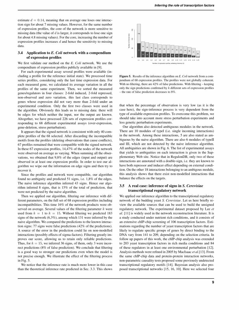
3 RESULTSIn perturbation experiments, gene responses are observed follow-ing changes of external conditions (temperature, nutritional stress,etc.) or following gene inactivations, knock-outs or overexpression.When expression profile is available for all the genes in the net-work we say that we have a complete profile, otherwise the profileis partial (data is missing). The effect of gene deletions is modelledas the one of inactivations, which is imposing negative gene varia-tions. Thus, we may say that we deal with perturbation experimentsthat do not change the topology of the network. An experiment inwhich topology is changed would be to record the effect of stresseson mutants; this possibility will be discussed elsewhere.
In order to validate our formal approach, we evaluate the per-centage of the network that might be recovered from a reasonablenumber of perturbation experiments. We first provide theoreticallimits for the percentage of recovered signs. These limits depend onthe topology of the network. For the transcriptional network of E.Coli, these limits are estimated first by a deterministic and then bya statistical algorithm. The statistical approach uses artificial ran-dom data. Then we combine expression profiles with a publiclyavailable structure of E. Coli network, and compute the percent-age of recovered signs. Finally, we combine real expression profileswith chIP-chip data on S. Cerevisiae, and evaluate the percentage ofrecovered signs in a real setting.
On computational ground, we check that our algorithms are ableto handle large scale data, as produced by high-throughput mea-surement techniques (expression arrays, chIP-chip data). This isdemonstrated in the following by considering networks of more thanseveral thousand genes.
3.1 Stress perturbation experiments: how many do youneed ?
For any given network topology, even when considering all possibleexperimental perturbations and expression profiles, there are signsthat can not be determined (see Table 2). Sign inference has thusa theoretical limit that we call theoretical percentage of recoveredsigns. This limit is unique for a given network topology. If onlysome perturbation experiments are available, and/or data is missing,the percentage of inferred signs will be lower. For a given numberN of available expression profiles, the average percentage of recov-ered signs is defined over all sets of N different expression profilescompatible with the qualitative constraints Eqs. (1) and (2).
In this section, we calculate and comment the theoretical andthe average percentages of recovered signs for the transcriptionalnetwork of E. Coli.
We first validate our method on the E. Coli network. We build theinteraction graph corresponding to E. Coli transcriptional network,using the publicly available RegulonDB [6] as our reference. Foreach transcriptional regulation A → B we add the correspondingarrow between genes A and B in the interaction graph. This graphwill be referred to as the unsigned interaction graph.
From the unsigned interaction graph of E. Coli, we build thesigned interaction graph, by annotating the edges with a sign. Mostof the time, the regulatory action of a transcription factor is availablein RegulonDB. When it is unknown, or when it depends on the levelof the transcription factor itself, we arbitrarily choose the value +for this regulation. This provides a graph with 1529 nodes and 3802edges, all edges being signed. The signed interaction graph is usedto generate complete expression profiles that simulate the effect ofperturbations. More precisely, a perturbation experiment is repre-sented by a set of gene expression variations {Xi}i=1,...,n. Thesevariations are not entirely random: they are constrained by Eqs.(1)and (2). Then we forget the signs of network edges and we computethe qualitative system with the signs of regulations as unknowns.
The theoretical maximum percentage of inference is given by thenumber of signs that can be recovered assuming that expression pro-files of all conceivable perturbation experiments are available. Wecomputed this maximum percentage by using constraint solvers (thealgorithm is given in Sec. 6). We found that at most 40.8% of thesigns in the network can be inferred, corresponding to Mmax =1551 edges.
However, this maximum can be obtained only if all conceivable(much more than 250) perturbation experiments are done, which isnot possible. We performed computations to understand the influ-ence of the number of experiments N on the inference. For eachvalue of N , where N grows from 5 to 200, we generated 100 sets ofN random expression profiles. Each time our inference algorithm isused to recover signs. Then, the average percentage of inference iscalculated as a function of N . The resulting statistics are shown inFig. 2.
When the number of experiments (X-axis) equals 1, the valueM1 = 609 corresponds to the average number of signs inferredfrom a single perturbation experiment. These signs correspond to
6

Inferring the role of transcription factors
20 40 60 80 100 120 140 160 180 2000.15
0.2
0.25
0.3
0.35
fract
ion
of in
fere
nce
number of expression profiles
whole network 1529 nodes 3802 edges
500 1000 1500 2000
0.25
0.3
0.35
0.4
0.45
fract
ion
of in
fere
nce
number of expression profiles
Core of the network 28 nodes, 57 edges
Figure 2. (Both) Statistics of inference on the regulatory network of E. Coli from complete expression profiles. The signed interaction graph is used torandomly generate sets of X artificial expression profiles which cover the whole network (complete expression profile). Each set of artificial profiles is thenused with the unsigned interaction graph to recover regulatory roles. X-axis: number of expression profiles in the dataset. Y-axis: percentage of recoveredsigns in the unsigned interaction graph. This percentage may vary for a fixed number of expression profile in a set. Instead of plotting each dot correspondingto a set, we represent the distribution by boxplots. Each boxplot vertically indicates the minimum, the first quartile, the median, the third quartile andthe maximum of the empiric distribution. Crosses show outliers (exceptional data points). The continuous line corresponds to the theoretical predictionY = M1 + M2(1 − (1 − p)X), where M1 stands for the number of signs that should be inferred from any expression profile (that is, inferred by the naiveinference algorithm); and M2 denotes the number of signs that could be inferred with a probability p.(Left) Statistics of inference for the whole E. Coli transcriptional network. We estimate that at most 37, 3% of the network can be inferred from a limitednumber of different complete expression profiles. Among the inferred regulations, we estimate to M1 = 609 the number of signs that should be inferred fromany complete expression profile. The remaining M2 = 811 signs are inferred with a probability estimated to p = 0.049. Hence, 30 perturbation experimentsare enough to infer 30% of the network.(Right) Statistics of inference for the core of the former graph (see definition of a core in the text). An estimation gives M1 = 18 and M2 = 9 so that themaximum rate of inference is 47, 3%. Since p = 0.0011, the number of expression profiles required to obtain a given percentage of inference is much greaterthan in the whole network.
single incoming regulatory interactions and are thus within thescope of the naive inference algorithm. We deduce that the naiveinference algorithm allows to infer on average 18% of the signs inthe network.
Surprisingly, by using our method we can significantly improvethe naive inference, with little effort. For the whole E. Coli net-work it appears that a few expression profiles are enough to infer asignificant percentage of the network. More precisely, 30 differentexpression profiles may be enough to infer one third of the network,that is about 1200 regulatory roles. Adding more expression profilescontinuously increases the percentage of inferred signs. We reacha plateau close to 37,3% (this corresponds to M = 1450 signedregulations) for N = 200.
The saturation aspect of the curve in Fig. 2 is compatible withtwo hypotheses. According to the first hypothesis, on top of theM1 single incoming regulations (that can be inferred with a sin-gle expression profile), there are M2 interactions whose signs areinferred with more than one expression profile. On average, a sin-gle expression profile determines with probability p < 1 the sign ofinteractions of the latter category. According to the second hypoth-esis, the contributions of different experiments to the inference ofthis type of interactions are independent. Thus, the average numberof inferred signs is M(N) = M1 + M2(1 − (1 − p)N ). The twonumbers satisfy M1 + M2 < E (E is the total number of edges),meaning that there are edges whose signs can not be inferred.
According to this estimate the position of the plateau is M =M1 + M2 and should correspond to the theoretical maximum per-centage of inferred signs Mmax. Actually, M < Mmax. Thedifference, although negligible in practice (to obtain Mmax onehas to perform N > 1015 experiments) suggests that the plateauhas a very weak slope. This means that contributions of differentexperiments to sign inference are weakly dependent.
The values of M1, M2, p estimate the efficiency of our method:large p,M1,M2 mean small number of expression profiles neededfor inference. For the E. Coli full transcriptional network we havep = 0.049 per observation. This means that we need about 20profiles to reach half of the theoretical limit of our approach.
3.2 Inferring the core of the networkObviously, not all interactions play the same role in the network.The core is a subnetwork that naturally appears for computationalpurpose and plays an important role in the system. It consists of alloriented loops and of all oriented chains leading to loops. All ori-ented chains leaving the core without returning are discarded whenreducing the network to its core. Acyclic graphs and in particulartrees have no core. The main property of the core is that if a systemof qualitative equations has no solution, then the reduced systembuilt from its core also have no solution. Hence it corresponds tothe most difficult part of the constraints to solve. It is obtained byreduction techniques that are very similar to those used in [31] (seedetails in Sec. 6). As an example, the core of E. Coli network onlyhas 28 nodes and 57 edges. It is shown in Fig. 3.
We applied the same inference process as before to this graph. Notsurprisingly, we noticed a rather different behavior when inferringsigns on a core graph than on a whole graph as demonstrated in Fig.2. In this case we need much more experiments for inference: sets ofexpression profiles contain from N = 50 to 2000 random profiles.
Two observations can be made from the corresponding statisticsof inference. First as can be seen on X-axis, a much greater num-ber of experiments is required to reach a comparable percentage ofinference. Correspondingly, the value of p is much smaller than forthe full network. This confirms that the core is much more difficultto infer than the rest of network. Second, Fig. 2. displays a muchless continuous behavior. More precisely, it shows that for the core,
7

P. Veber a, C. Guziolowski a, M. Le Borgneb, O. Radulescua,c, A. Siegeld
5 10 15 20 25 30 35
0.26
0.27
0.28
0.29
0.3
0.31
0.32
0.33
fract
ion
of in
fere
nce
% of missing values
d=0.14
5 10 15 20 25 30 35 40 45 50
0.1
0.15
0.2
0.25
0.3
fract
ion
of in
fere
nce
% of missing values
d=0.21
5 10 15 20 25 30 35 40 45 50
0.2
0.25
0.3
0.35
fract
ion
of in
fere
nce
% of missing values
d=0.36
Figure 4. (All) Statistics of inference on the regulatory network of E. Coli from partial expression profiles. The setting is the same than in Fig. (2), except forthe cardinal of an expression profile which is set to a given value, and for the variable on X-axis which is the percentage of missing values in the expressionprofile. In each case, the dependence between average percentage of inference and percentage of missing values is qualitatively linear. The continuous linecorresponds to the theoretical prediction Mi = Mmax
i − d ∗ f ∗Mtotal, where d is the number of signs interactions that are no longer inferred when a nodeis not observed, Mmax
i is the number of inferred interactions for complete expression profiles (no missing values), Mtotal is the total number of nodes andf is the fraction of unobserved nodes.(Left) Statistics for the whole network (the inference is supposed to be performed from 30 random expression profiles). We estimate d = 0.14, meaning thaton average, one loses one interaction sign for about 7 missing values.(Middle) Statistics for the core network (the inference is supposed to be performed from 30 random expression profiles). We estimate d = 0.21 ; the core ofthe network however is more sensitive to missing data.(Right) Statistics for the core network (the inference is supposed to be performed from 200 random expression profiles). We estimate d = 0.35. Hence,increasing the number of expression profiles increases sensitivity to missing data.
Figure 3. Core of E. Coli network. It consists of all oriented loops andof all oriented chains leading to loops. The core contains the dynamicalinformation of the network, hence sign edges are more difficult to infer.
different perturbations experiments have strongly variable impact onsign inference. For instance, the experimental maximum percentageof inference (27 signs over 58) can be obtained already from about400 expression profiles. But most of datasets with 400 profiles inferonly 22 signs.
This suggests that not only the core of the network is more dif-ficult to infer, but also that a brute force approach (multiplying thenumber of experiments) may fail as well. This situation encourageus to apply experiment design and planning, that is, computationalmethods to minimize the number of perturbation experiments whileinferring a maximal number of regulatory roles.
This also illustrates why our approach is complementary to dy-namical modelling. In the case of large scale networks, when aninteraction stands outside the core of the graph, then an inferenceapproach is suitable to infer the sign of the interaction. However,
when an interaction belongs to the core of the network, then morecomplex behaviors occur: for instance, the result of a perturbationon the variation of the products might depend on activation thresh-olds. Then, a precise modelling of the dynamical behavior of thispart of the network should be performed [32].
3.3 Influence of missing dataIn the previous paragraph, we made the assumption that all proteinsin the network are observed. That is, for each experiment each nodeis assigned a value in {+, 0, –}. However, in real measurement de-vices, such as expression profiles, a part of the values is discardeddue to technical reasons. A practical method for network inferenceshould cope with missing data.
We studied the impact of missing values on the percentage of in-ference. For this, we have considered a fixed number of expressionprofiles (N = 30 for the whole E. Coli network, N = 30 andN = 200 for its core). Then, we have randomly discarded a growingpercentage of proteins in the profiles, and computed the percentageof inferred regulations. The resulting statistics are shown in Fig. 4.
In both cases (whole network and core), the dependency betweenthe average percentage of inference and the percentage of missingvalues is qualitatively linear. Simple arguments allow us to find ananalytic dependency. If not observing a node implies losing infor-mation on d interaction signs, we are able to obtain the followinglinear dependency Mi = Mmax
i − d ∗ f ∗Mtotal, where Mmaxi is
the number of inferred interactions for complete expression profiles(no missing values), Mtotal is the total number of nodes, and f isthe fraction of unobserved nodes. In order to keep Mtotal non neg-ative, d must decrease with f . Our numerical results imply that theconstancy of d and the linearity of the above dependency extend torather large values of f . This indicates that our qualitative inferencemethod is robust enough for practical use. For the full network we
8
Inferring the role of transcription factors
estimate d = 0.14, meaning that on average one loses one interac-tion sign for about 7 missing values. However, for the same numberof expression profiles, the core of the network is more sensitive tomissing data (the value of d is larger, it corresponds to lose one signfor about 4.8 missing values). For the core, increasing the number ofexpression profiles increases d and hence the sensitivity to missingdata.
3.4 Application to E. Coli network with a compendiumof expression profiles
We first validate our method on the E. Coli network. We use thecompendium of expression profiles publicly available in [9].
For each experimental assay several profiles were available (in-cluding a profile for the reference initial state). We processed timeseries profiles, considering only the last time expression data. Foreach measured gene, we calculated its average variation in all theprofiles of the same experiment. Then, we sorted the measuredgenes/regulators in four classes: 2-fold induced, 2-fold repressed,non-observed and zero variation, this last class corresponds togenes whose expression did not vary more than 2-fold under anexperimental condition. Only the first two classes were used inthe algorithm. Obviously this leads us to missing data: there willbe edges for which neither the input, nor the output are known.Altogether, we have processed 226 sets of expression profiles cor-responding to 68 different experimental assays (over-expression,gene-deletion, stress perturbation).
It appears that the signed network is consistent with only 40 com-plete profiles of the 68 selected. After discarding the incompatiblemotifs from the profiles (deleting observations that cause conflicts),67 profiles remained that were compatible with the signed network.In these 67 expression profiles, 14,47% of the nodes of the networkwere observed on average as varying. When summing all the obser-vations, we obtained that 9,8% of the edges (input and output) areobserved in at least one expression profile. In order to test our al-gorithm we wipe out the information on edge signs and then try torecover it.
Since the profiles and network were compatible, our algorithmfound no ambiguity and predicted 51 signs, i.e. 1,8% of the edges.The naive inference algorithm inferred 43 signs. Hence our algo-rithm inferred 8 signs, that is 15% of the total of prediction, thatwere not predicted by the naive algorithm.
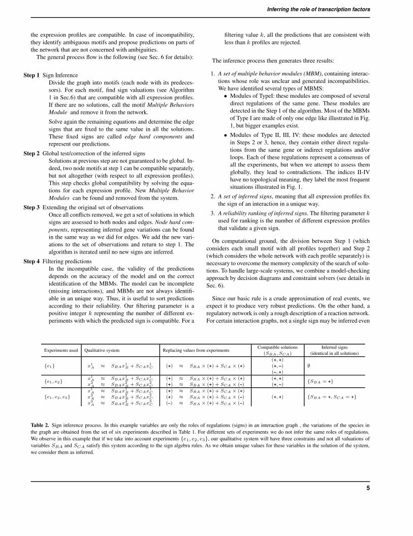
Then we applied our algorithm, filtering our inference with dif-ferent parameters, on the full set of 68 expression profiles includingincompatibilities. This time 16% of the network products were ob-served on average. Several values of the filtering parameter k wereused from k = 1 to k = 15. Without filtering we predicted 183signs of the network (6,3%), among which 131 were inferred by thenaive algorithm. We compared the predictions to the known interac-tion signs: 77 signs were false predictions (42% of the predictions).A source of the error in the prediction could lie on non-modelledinteractions (possibly effects of sigma-factors). Filtering greatly im-proves our score, allowing us to retain only reliable predictions.Thus, for k = 15, we inferred 36 signs, of them, only 3 were incor-rect predictions (8% of false prediction). We conclude that filteringis a good way to stronger our predictions even when the model isnot precise enough. We illustrate the effect of the filtering processin Fig. 5.
We notice that the inference rate is much more lower in this casethan the theoretical inference rate predicted in Sec. 3.3. This shows
k.1 k.2 k.3 k.4 k.5 k.6 k.7 k.8 k.9 k.10 k.11 k.12 k.13 k.14 k.15
Number of expression profiles validating inference (k)
Num
ber o
f inf
erre
d ro
les
050
100
150
77
106
32
54
29
52
28
49
24
50
21
49
21
48
21
47
20
47
19
44
19
43
16
44
14
42
9
41
3
33
Figure 5. Results of the inference algorithm on E. Coli network from a com-pendium of 68 expression profiles. The profiles were not globally coherent.With no filtering, there are 42% of false predictions. With filtering – keepingonly the sign predictions confirmed by k different sets of expression profiles– the rate of false prediction decreases to 8%.
that when the percentage of observation is very low (as it is thecase here), the sign-inference process is very dependent from thetype of available expression profiles. To overcome this problem, weshould take into account more stress perturbation experiments andless genetic perturbation experiments.
Our algorithm also detected ambiguous modules in the network.There are 10 modules of typeI (i.e. single incoming interactions)in the network. Among these interactions, 5 are also stated as am-biguous by the naive algorithm. There are also 6 modules of typeIIand III, which are not detected by the naive inference algorithm.All ambiguities are shown in Fig. 6. The list of experimental assaysthat yields to ambiguities on each interaction is given in the Sup-plementary Web site. Notice that in RegulonDB, only two of theseinteractions are annotated with a double-sign, i.e. they are known tohave both repressor and inducer effect depending on external condi-tion. On the other 18 interactions belonging to an ambigous module,this analysis shows that there exist non-modelled interactions thatbalance the effects on the targets.
3.5 A real case: inference of signs in S. Cerevisiaetranscriptional regulatory network
We applied our inference algorithm to the transcriptional regulatorynetwork of the budding yeast S. Cerevisiae. Let us here briefly re-view the available sources that can be used to build the unsignedregulatory network. The experimental dataset proposed by Lee etal. [11] is widely used in the network reconstruction literature. It isa study conducted under nutrient rich conditions, and it consists ofan extensive chIP-chip screening of 106 transcription factors. Esti-mations regarding the number of yeast transcription factors that arelikely to regulate specific groups of genes by direct binding to theDNA vary from 141 to 209, depending on the selection criteria. Infollow up papers of this work, the chIP-chip analysis was extendedto 203 yeast transcription factors in rich media conditions and 84of these regulators in at least one environmental perturbation [12].Analysis methods were refined in 2005 by MacIsaac et al.[13]. Fromthe same chIP-chip data and protein-protein interaction networks,non-parametric causality tests proposed some previously undetectedtranscriptional regulatory motifs [14]. Bayesian analysis also pro-posed transcriptional networks [15, 16, 10]. Here we selected four
9

P. Veber a, C. Guziolowski a, M. Le Borgneb, O. Radulescua,c, A. Siegeld
Figure 6. Interactions in the regulatory network of E. Coli that are ambigu-ous with a compendium data of expression profiles [9]. For each interaction,there exist at least two expression profiles that do not predict the same signon the interaction. In this subnetwork, only 2 interactions (red edges) areannotated with a double-sign in RegulonDB.
of these sources. All networks are provided in the SupplementaryWeb site.
(A) The first network consists in the core of the transcriptionalchIP-chip regulatory network produced in [11]. Starting fromthe full network with a p-value of 0.005, we reduced it tothe set of nodes that have at least one output edge. This net-work was already studied in [31]. It contains 31 nodes and 52interactions.
(B) The second network contains all the transcriptional interactionsbetween transcription factors shown by [11] with a p-valuebelow 0.001. It contains 70 nodes and 96 interactions.
(C) The third network is the set of interactions among transcriptionfactors as inferred in [13] from sequence comparisons. We have
considered the network corresponding to a p-value of 0.001and 2 bindings (83 nodes, 131 interactions).
(D) The last network contains all the transcriptional interactionsamong genes and regulators shown by [11] with a p-valuebelow 0.001. It contains 2419 nodes and 4344 interactions.
3.5.1 Inference process with gene-deletion expression profilesWe first applied our inference algorithm to the large-scale network(D) extracted from [11] using a panel of expression profiles for 210gene-deletion experiments [40]. The information given by this panelis quite small, since 1, 6% of all the products in the network is onaverage observed, and 12% of the edges (input and output) of thenetwork are observed in at least one expression profile. Using thisdata, we obtain 162 regulatory roles.
We validated our prediction with a literature-curated network onYeast [41]. We found that among the 162 sign-predictions, 12 werereferenced with a known interaction in the database, and 9 with agood sign.
Gene-deletion expression profiles were used so we could compareour results to path analysis methods [23, 20] since the latter can onlybe applied to knock-out data (http://chianti.ucsd.edu/idekerlab/).Other sign-regulation inference methods need either other sourcesof gene-regulatory information (promoter binding information,protein-protein information), or time-series data to be performed[15, 18, 10].
Before comparing our inference results to the work of Yeang etal., we tested the compatibility between their inferred network withthe 210 gene-deletion experiments. We obtained that their networkwas incompatible with 28 of the 210 experiments. The comparisonof both results showed us that the method of Yeang et al. infers234 roles of widely connected paths, while our method infers 162roles in the branches of the network. Both results intersect on 17interactions, and no contradiction in the inferred role was reported.An illustration of these results is given in the Supplementary Website.
This suggests that our approach is complementary to path analy-sis methods. Our explanation is the following: In [23, 20], networkinference algorithms identify probable paths of physical interac-tions connecting a gene knockout to genes that are differentiallyexpressed as a result of that knockout. This leads to search for thesmallest number of interactions that carry the largest information inthe network. Hence, inferred interactions are located near the core
ExperimentIdentifier
Description Reference
E1 Diauxic Shift [30]E2 Sporulation [33]E3 Expression analysis of Snf2 mutant [34]E4 Expression analysis of Swi1 mutant [34]E5 Pho metabolism [35]E6 Nitrogen Depletion [28]E7 Stationary Phase [28]E8 Heat Shock from 21◦C to 37◦C [28]E9 Heat Shock from 17◦C to 37◦C [28]
ExperimentIdentifier
Description Reference
E10 Wild type response to DNA-damaging agents [36]E11 Mec1 mutant response to DNA-damaging agents [36]E12 Glycosylation defects on gene expression [37]E13 Cells grown to early log-phase in YPE [29]
(Rich medium with 2% of Ethanol)E14 Cells grown to early log-phase in YPG [29]
(Rich medium with 2% of Glycerol)E15 Titratable promoter alleles - Ero1 mutant [38]
Table 3. List of genome expression experiments of S. Cerevisiae used in the inference process. Experiments contain information on steady state shift and theircurated data is available in SGD (Saccharomyces Genome Database) [39].
10

Inferring the role of transcription factors
Interaction network Nodes Edges
Averagenumber ofobserved
nodes
In/Outobservedsimulnat.
Inferredsigns
MBM Int.TypeI
MBM Int.Type
II,III,IV
Total Inf.rate
Predictionsof thenaive
algorithm(A) Core of
Lee transcriptionalnetwork[11, 31]
31 52 28% 4611
(21.1%)3
(5.7%)0 26.8% 11%
(B) ExtendedLee transcriptional
network[11]
70 96 26% 7029
(30.2%)7
(7.2%)0 37.4% 15,6%
(C) Inferred network[12, 13]
threshold = 0.001 ;bindings=2
83 131 33% 9121
(16%)4
(3%)0 19% 11%
(D) Global transcriptionalnetwork [11]
p-value = 0.0012419 4344 30% 2270
631(14.5%)
198(4.5%)
filter k=3
281(6.5%)no filter
463(11%)
32% 13.9%
Table 4. Budding yeast transcriptional regulatory networks on which the sign inference algorithm was applied. For each network 14 or 15 different expressionprofiles were used for calculating the inference. The set of observations provided by one expression profile, was composed by at least two expressed/repressed(ratio over/under 2-fold) genes of the network. The Input/Output observed simultaneously column, is an indicator of the maximum possible number of sign-inferred interactions. There are three different inference results: Inferred signs, signs fixed in a unique way by all experiments, MBM Interactions of TypeI,the set of non-repeated interactions that belong to all the multiple behavior modules of TypeI detected, and MBM Interactions of TypeII,II,IV, the number ofnon-repeated interactions belonging to MBM of Type II,III,IV. For all the inference results a percentage concerning the total number of edges of the network,is calculated. The Total inference rate represents the percentage of the total number of edges that was inferred (inferred signs plus interactions in MBM). It iscompared to the results of the naive algorithm.
of the network (even though not exactly in the core). On the con-trary, as we already detailed it, the combinatorics of interaction inthe core of the network is too intricate to be determined from a fewhundreds of parse expression profiles with our algorithm, and weconcentrate on interactions around the core.
3.5.2 Inference with stress perturbation expression profiles Inorder to overcome the problem raised by the small amount of in-formation contained in [40], we have selected stress perturbationexperiments. This data corresponds to curated information avail-able in SGD (Saccharomyces Genome Database) [39]. When timeseries profiles were available, we selected the last time expressionarray. Therefore, we collected and treated 15 sets of arrays describedin Table 3. For each expression array, we sorted the measuredgenes/regulators in four classes: 2-fold induced, 2-fold repressed,non-observed and zero variation. We were only interested in the ex-pression of genes that belong to any of the four networks we studied.Full datasets are available in the Supplementary Web site.
As for E. Coli network, it appeared that all networks (A), (B), (C)and (D) are not consistent with the whole set of expression arraysand ambiguities appeared. We performed our inference algorithm.We identified motifs that hold ambiguities, and we marked them asMultiple Behavior Modules of type I, II and III, as described in Sec.3.1. The algorithm also generates a set of inferred signs. Then weapplied the filtered algorithm (with filter k = 3) to the large-scalenetwork (D).
We obtain our total inference rate adding the number of inferredsigns fixed in a unique way to the number of non-repeated inter-actions that belong to all the detected multiple behavior modulesand dividing it by the number of edges in the network. In Table4 we show the inference rate for Networks (A), (B), (C) and (D).Depending on the network, the rate of inference goes from 19% to
37%. Hence, the rates of inference are very similar to the theoreti-cal rates obtained for E. Coli network, still with a small number ofperturbation experiments (14 or 15).
We validated the inferred interaction by comparing them to theliterature-curated network published in [41]. We first obtained thatamong the 631 interactions predicted when no filtering is applied,23 are annotated in the network, and seven annotations are con-tradictory to our predictions. However, among the 198 interactionspredicted with a filter parameter k = 3, 19 are annotated in the net-work, and only one annotation is contradictory to our predictions.As in the case of E. Coli, we conclude that filtering is a good way tomake strong predictions even when the model is not precise enough.We also compared the sign predictions to the predictions of the naiveinference algorithm. We found that the naive algorithm usually pre-dicts half of the signs that we obtain. In Fig. 7 we illustrate theinferred interactions for Network (B), that is, the Transcriptionalnetwork among transcription factors produced in [11].
As mentioned already, the algorithm identified a large number ofambiguities. The exhaustive list of MBM is given in the Supple-mentary Web site. We notice that MBM of Type I are detected inthe four networks; we list the Type I modules of size 2 found for thenetworks (A), (B) and (C) in Table 5. In contrast, MBM of Type II,III and IV are only detected, in an important number, for Network(D) following the distribution: 85.4% of Type II, 5.3% of Type IIIand 9.3% of Type IV. In network (D), all the results were obtainedafter 3 iterations of the inference algorithm. For each MBM, a pre-cise biological study of the species should allow to understand theorigin of the ambiguity: error in expression data, missing interac-tion in the model or changing in the sign of the interaction duringthe experimentation.
11

P. Veber a, C. Guziolowski a, M. Le Borgneb, O. Radulescua,c, A. Siegeld
Figure 7. Transcriptional regulatory network among transcription factors (70 nodes, 96 edges) extracted from [11]. A total of 29 interactions were inferred:arrows in green, respectively in red, correspond to positive, respectively negative, interactions inferred; blue arrows correspond to the detected multiplebehavior modules of TypeI. Diagram layout is performed automatically using the Cytoscape package [42].
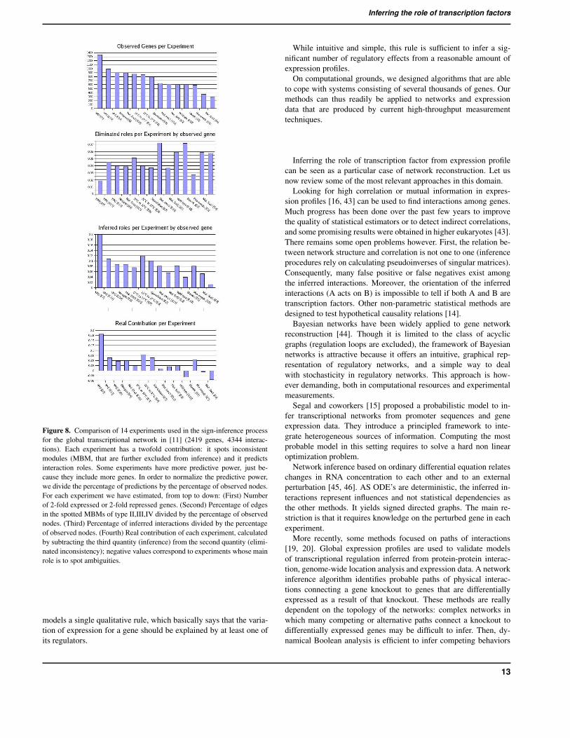
3.6 Contribution of expression profiles to the inferenceIn order to evaluate the contribution of the 14 experiments used forthe inference in the global network provided in [11] (2419 nodesand 4344 arcs), we addressed the following question: assuming thatall inferred roles are correct, which is the experiment that causesthe suppression of most of the inferred roles? For example, in Fig.1 expression data related to YPD Broth to Stationary Phase [28],caused the suppression of the inferred interactions of the module ofType II.
We compared the 14 expression profiles according to the MBMof TypeII, III and IV that are detected by using an element of thedataset. MBM of TypeI are not included in this computation, since
they do not invalidate any interaction role, as no interaction role isinferred before their detection. The results of this comparison areshown in Fig. 8. The fourth chart illustrates that the real contribu-tion of each expression profile does not depends on the amount ofobservations.
4 DISCUSSIONIn this work we show how a qualitative reasoning framework canbe used to infer the role of transcription factor based on expressionprofiles. The regulatory effect of a transcription factor on its targetgenes can either be an activation or a repression. Our framework
Interaction network Actor Target Experiment 1 Experiment 2
Core of Leenetwork
YAP6GRF10PDH1
CIN5MBP1MSN4
Expression during Sporulation [33]YPD Broth to Stationary Phase [28]
Nitrogen Depletion [28]
YPD Broth to Stationary Phase [28]Mec1 mutant + Heat [36]Heat shock 21 to 37 [28]
Extended Leenetwork
YAP6RAP1SKN7PHD1RAP1PHD1HAP4
CIN5SIP4
NRG1SOK2RCS1MSN4PUT3
Expression during Sporulation [33]Expression during Sporulation [33]YPD Broth to Stationary Phase [28]
Heat shock 21 to 37 [28]Wild type + Heat [36]
Nitrogen Depletion [28]Expression during the diauxic shift [30]
YPD Broth to Stationary Phase [28]Expression during the diauxic shift [30]Expression during the diauxic shift [30]
YPD Broth to Stationary Phase [28]Transition from fermentative to glycerol-based respiratory growth [29]
Heat shock 21 to 37 [28]Snf2 mutant, YPD [34]
MacIssacinferred network
SWI5SKN7NRG1NRG1
ASH1NRG1YAP7GAT3
Expression regulated by the PHO pathway [35]YPD Broth to Stationary Phase [28]
Expression regulated by the PHO pathway [35]Glycosylation [37]
YPD Broth to Stationary Phase [28]Nitrogen Depletion [28]
Transition from fermentative to glycerol-based respiratory growth [29]Transition from fermentative to glycerol-based respiratory growth [29]
Table 5. Result of the diagnosis procedure for three networks related to budding yeast S. Cerevisiae (core, extended transcriptional networks of Lee, inferrednetwork of MacIsaac). We found ambiguities between single interactions and pairs of data (we call them Multiple Behavior Modules of Type I and size 2). Foreach ambiguous interaction found, we list two experiments that deduce a different role of interaction among these genes.
12
Inferring the role of transcription factors
Figure 8. Comparison of 14 experiments used in the sign-inference processfor the global transcriptional network in [11] (2419 genes, 4344 interac-tions). Each experiment has a twofold contribution: it spots inconsistentmodules (MBM, that are further excluded from inference) and it predictsinteraction roles. Some experiments have more predictive power, just be-cause they include more genes. In order to normalize the predictive power,we divide the percentage of predictions by the percentage of observed nodes.For each experiment we have estimated, from top to down: (First) Numberof 2-fold expressed or 2-fold repressed genes. (Second) Percentage of edgesin the spotted MBMs of type II,III,IV divided by the percentage of observednodes. (Third) Percentage of inferred interactions divided by the percentageof observed nodes. (Fourth) Real contribution of each experiment, calculatedby subtracting the third quantity (inference) from the second quantity (elimi-nated inconsistency); negative values correspond to experiments whose mainrole is to spot ambiguities.
models a single qualitative rule, which basically says that the varia-tion of expression for a gene should be explained by at least one ofits regulators.
While intuitive and simple, this rule is sufficient to infer a sig-nificant number of regulatory effects from a reasonable amount ofexpression profiles.
On computational grounds, we designed algorithms that are ableto cope with systems consisting of several thousands of genes. Ourmethods can thus readily be applied to networks and expressiondata that are produced by current high-throughput measurementtechniques.
Inferring the role of transcription factor from expression profilecan be seen as a particular case of network reconstruction. Let usnow review some of the most relevant approaches in this domain.
Looking for high correlation or mutual information in expres-sion profiles [16, 43] can be used to find interactions among genes.Much progress has been done over the past few years to improvethe quality of statistical estimators or to detect indirect correlations,and some promising results were obtained in higher eukaryotes [43].There remains some open problems however. First, the relation be-tween network structure and correlation is not one to one (inferenceprocedures rely on calculating pseudoinverses of singular matrices).Consequently, many false positive or false negatives exist amongthe inferred interactions. Moreover, the orientation of the inferredinteractions (A acts on B) is impossible to tell if both A and B aretranscription factors. Other non-parametric statistical methods aredesigned to test hypothetical causality relations [14].
Bayesian networks have been widely applied to gene networkreconstruction [44]. Though it is limited to the class of acyclicgraphs (regulation loops are excluded), the framework of Bayesiannetworks is attractive because it offers an intuitive, graphical rep-resentation of regulatory networks, and a simple way to dealwith stochasticity in regulatory networks. This approach is how-ever demanding, both in computational resources and experimentalmeasurements.
Segal and coworkers [15] proposed a probabilistic model to in-fer transcriptional networks from promoter sequences and geneexpression data. They introduce a principled framework to inte-grate heterogeneous sources of information. Computing the mostprobable model in this setting requires to solve a hard non linearoptimization problem.
Network inference based on ordinary differential equation relateschanges in RNA concentration to each other and to an externalperturbation [45, 46]. AS ODE’s are deterministic, the inferred in-teractions represent influences and not statistical dependencies asthe other methods. It yields signed directed graphs. The main re-striction is that it requires knowledge on the perturbed gene in eachexperiment.
More recently, some methods focused on paths of interactions[19, 20]. Global expression profiles are used to validate modelsof transcriptional regulation inferred from protein-protein interac-tion, genome-wide location analysis and expression data. A networkinference algorithm identifies probable paths of physical interac-tions connecting a gene knockout to genes that are differentiallyexpressed as a result of that knockout. These methods are reallydependent on the topology of the networks: complex networks inwhich many competing or alternative paths connect a knockout todifferentially expressed genes may be difficult to infer. Then, dy-namical Boolean analysis is efficient to infer competing behaviors
13

P. Veber a, C. Guziolowski a, M. Le Borgneb, O. Radulescua,c, A. Siegeld
on models containing tens of products [20, 31]. The main restric-tion to this method is that expression profiles have to result from agene-deletion perturbation.
In this work, we rely on a discrete modeling framework, whichconsists in calculating an over-approximation of the set of possi-ble observations, by abstracting noisy quantitative values into morerobust properties. In contrast, statistical methods deal with experi-mental noise by explicitly modeling the noise distribution, providedenough measurements are available – which usually means hun-dreds of independent experiments. Moreover while most methodsreport the most likely model given the data, we describe the (pos-sibly huge) set of consistent experimental behaviors with a systemof qualitative constraints. Then we look for invariants in this set. Inthe worst case, not a single regulatory effect can be deduced fromthe set of constraints, whereas computing the most likely model pro-vides with signs for all regulations. However, we expect the inferredregulations to be more robust. Another crucial difference is that thesystem of constraints might have no solution at all. In combinationwith a diagnosis procedure, we illustrated how this approach can bea relevant tool for the curation of network databases.
We compared our inference approach to a naive inference algo-rithm and path analysis methods introduced in [23, 20]. As detailedabove, all other inference methods need additional information toinfer the signs of regulations. We found that both our algorithmand path analyses infer non-trivial interactions. Both approaches arecomplementary: path analyses identify coupled with boolean analy-sis allows to infer the signs of interactions located in paths that areconnected to a large number of targets; whereas our method yieldsinformation on paths connected to a quite small number of targets.Another difference is that paths analysis requires gene-deletion per-turbation expression profiles, while our method give better resultswith stress perturbation experiments (though it can be applied toany type of experiment).
Using simulations we investigated the dependence between thenumber of inferred signs and the number of available observations.Not surprisingly we noticed that the topology of the regulatory graphalone had a strong influence on the estimated relationship. Thiswas illustrated by computing statistics both on a complete regula-tory network and on its core, as defined in the Methods section.The complete network is characterized by an over-representationof feedback-free regulatory cascades, which are controlled by asmall number of transcription factors. In this setting, the numberof inferred signs grows quasi continuously with the number of ob-servations. In contrast, the core network does not obey the simplelaw “the more you observe, the better”: some expression profilesare clearly more informative than others. A challenging sequel tothis work deals with experimental planification: given some con-trol parameters, how to find the most informative experiments whilekeeping their number as low as possible ?
As a practical assessment of our method, we conducted sign in-ference experiments on E. Coli and S. Cerevisiae, using curatedexpression measurements, and regulatory networks either alreadypublished or based on chIP-chip data. When expression profilesmostly consisted in genetic perturbations, the inference rate wasquite low, even though comparable to the results of paths analysis[20]. When expression profiles consisted in stress perturbation, ourinference results corresponded to the theoretical rate of inference.
For smaller networks, of about 100 interactions, we were able to in-fer 20% of the regulatory roles. For bigger networks, of thousandsinteractions, we were only able to infer the 14%, however, a hugenumber of inconsistencies (that we called multiple behaviour mod-ules) were detected. Even if we were able to state some correctionsover the model or data, all our inferences and corrections proposeddepend on the model we worked with. If the orientation sense ofsome interaction was mistaken, our inferences will be mistaken aswell. In our opinion, what is even more relevant than correctly in-ferring signed regulations among genes is the ability to detect andisolate situations where different data sources are not consistent witheach other. Moreover, if we group some of the MBM found accord-ing to the common genes they share, it is possible to assign a higherrelevance to the correction of some specific interaction or data; inother words, it is possible to choose which of all the interactions isthe most inappropriate.
5 CONCLUSIONIn this work, we showed that our approach is suitable to infer reg-ulatory roles of transcription factor from a limited amount of data.More precisely, we could infer 30-40% of the networks we stud-ied from about 20-30 perturbation expression arrays. We believethat our approach is complementary to previous statistical meth-ods: while qualitative modeling is a less accurate description ofregulatory networks, it requires less data in order to make robustpredictions. Thus, it is more adapted to situations where diverse buteven limited expression profiles (some tens) are available, instead ofthe large panel of expression profiles usually needed for statisticalmethods.
We proposed a characterization of sub-networks that are moredifficult to infer, called the core of a network. We showed on sim-ulated data that in these core networks an unfeasible number ofexperiments is necessary to infer a small number of signs with highprobability. For these core networks, two different strategies maybe adopted. The first strategy is to build a more accurate model forthese restricted subnetworks, using dynamic modeling techniques(see ([32] for a review), The alternative is to develop experimentdesign in our qualitative framework: find suitable values for controlparameters to infer the maximum number of signs.
Finally, we illustrated another advantage of discrete modeling,namely that models can be submitted to exhaustive verification anddiagnosis. As we show it in this paper it is possible to reason on sys-tems with thousands of observations, constraints and variables, andprovide intuitive diagnosis representations automatically when ex-pression profiles happen to be ambiguous with the regulation model.As a follow-up to this work, we plan to deepen diagnosis represen-tation, and eventually propose automatic hypothesis generation forthe existence of defects.
6 METHODSProblem statement We consider the set of equations derived from a giveninteraction graph G:
Xki ≈
X
j→i
SjiXkj for 1 ≤ i ≤ n, 1 ≤ k ≤ r (4)
where Xki stands for the sign of variation of species i in experiment k, and
Sji the sign of the influence of species j on species i. Recall that the graph G
itself comes from chIP-chip experiments or sequence analysis. Using expres-sion arrays, we obtain an experimental value for some variables Xk
i , which
14
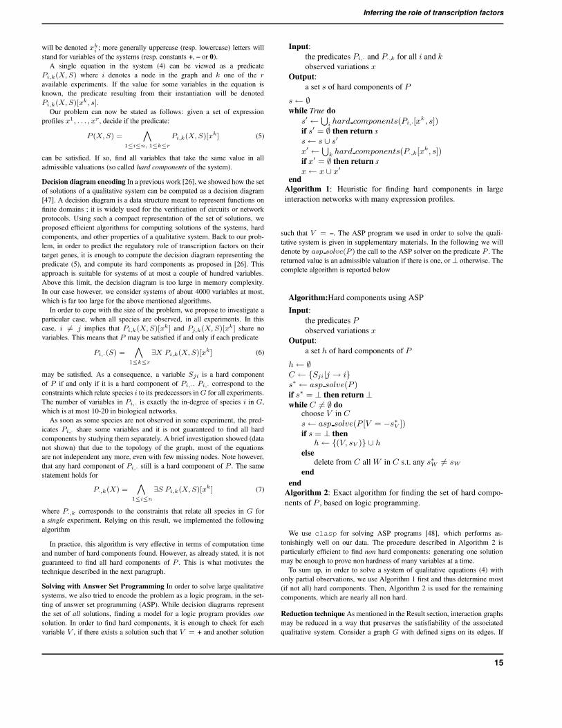
Inferring the role of transcription factors
will be denoted xki ; more generally uppercase (resp. lowercase) letters will
stand for variables of the systems (resp. constants +, – or 0).A single equation in the system (4) can be viewed as a predicate
Pi,k(X, S) where i denotes a node in the graph and k one of the r
available experiments. If the value for some variables in the equation isknown, the predicate resulting from their instantiation will be denotedPi,k(X, S)[xk, s].
Our problem can now be stated as follows: given a set of expressionprofiles x1, . . . , xr, decide if the predicate:
P (X,S) =^
1≤i≤n, 1≤k≤r
Pi,k(X, S)[xk] (5)
can be satisfied. If so, find all variables that take the same value in alladmissible valuations (so called hard components of the system).
Decision diagram encoding In a previous work [26], we showed how the setof solutions of a qualitative system can be computed as a decision diagram[47]. A decision diagram is a data structure meant to represent functions onfinite domains ; it is widely used for the verification of circuits or networkprotocols. Using such a compact representation of the set of solutions, weproposed efficient algorithms for computing solutions of the systems, hardcomponents, and other properties of a qualitative system. Back to our prob-lem, in order to predict the regulatory role of transcription factors on theirtarget genes, it is enough to compute the decision diagram representing thepredicate (5), and compute its hard components as proposed in [26]. Thisapproach is suitable for systems of at most a couple of hundred variables.Above this limit, the decision diagram is too large in memory complexity.In our case however, we consider systems of about 4000 variables at most,which is far too large for the above mentioned algorithms.
In order to cope with the size of the problem, we propose to investigate aparticular case, when all species are observed, in all experiments. In thiscase, i 6= j implies that Pi,k(X, S)[xk] and Pj,k(X, S)[xk] share novariables. This means that P may be satisfied if and only if each predicate
Pi,·(S) =^
1≤k≤r
∃X Pi,k(X, S)[xk] (6)
may be satisfied. As a consequence, a variable Sji is a hard componentof P if and only if it is a hard component of Pi,·. Pi,· correspond to theconstraints which relate species i to its predecessors in G for all experiments.The number of variables in Pi,· is exactly the in-degree of species i in G,which is at most 10-20 in biological networks.
As soon as some species are not observed in some experiment, the pred-icates Pi,· share some variables and it is not guaranteed to find all hardcomponents by studying them separately. A brief investigation showed (datanot shown) that due to the topology of the graph, most of the equationsare not independent any more, even with few missing nodes. Note however,that any hard component of Pi,· still is a hard component of P . The samestatement holds for
P·,k(X) =^
1≤i≤n
∃S Pi,k(X, S)[xk] (7)
where P·,k corresponds to the constraints that relate all species in G fora single experiment. Relying on this result, we implemented the followingalgorithm
In practice, this algorithm is very effective in terms of computation timeand number of hard components found. However, as already stated, it is notguaranteed to find all hard components of P . This is what motivates thetechnique described in the next paragraph.
Solving with Answer Set Programming In order to solve large qualitativesystems, we also tried to encode the problem as a logic program, in the set-ting of answer set programming (ASP). While decision diagrams representthe set of all solutions, finding a model for a logic program provides onesolution. In order to find hard components, it is enough to check for eachvariable V , if there exists a solution such that V = + and another solution
Input:the predicates Pi,· and P·,k for all i and k
observed variations x
Output:a set s of hard components of P
s← ∅while True do
s′ ←S
ihard components(Pi,·[x
k, s])if s′ = ∅ then return ss← s ∪ s′
x′ ←S
khard components(P·,k[xk, s])
if x′ = ∅ then return sx← x ∪ x′
endAlgorithm 1: Heuristic for finding hard components in largeinteraction networks with many expression profiles.
such that V = –. The ASP program we used in order to solve the quali-tative system is given in supplementary materials. In the following we willdenote by asp solve(P ) the call to the ASP solver on the predicate P . Thereturned value is an admissible valuation if there is one, or ⊥ otherwise. Thecomplete algorithm is reported below
Algorithm:Hard components using ASP
Input:the predicates P
observed variations x
Output:a set h of hard components of P
h← ∅C ← {Sji|j → i}s∗ ← asp solve(P )if s∗ = ⊥ then return ⊥while C 6= ∅ do
choose V in C
s← asp solve(P [V = −s∗V ])if s = ⊥ then
h← {(V, sV )} ∪ h
elsedelete from C all W in C s.t. any s∗W 6= sW
endend
Algorithm 2: Exact algorithm for finding the set of hard compo-nents of P , based on logic programming.
We use clasp for solving ASP programs [48], which performs as-tonishingly well on our data. The procedure described in Algorithm 2 isparticularly efficient to find non hard components: generating one solutionmay be enough to prove non hardness of many variables at a time.
To sum up, in order to solve a system of qualitative equations (4) withonly partial observations, we use Algorithm 1 first and thus determine most(if not all) hard components. Then, Algorithm 2 is used for the remainingcomponents, which are nearly all non hard.
Reduction technique As mentioned in the Result section, interaction graphsmay be reduced in a way that preserves the satisfiability of the associatedqualitative system. Consider a graph G with defined signs on its edges. If
15

P. Veber a, C. Guziolowski a, M. Le Borgneb, O. Radulescua,c, A. Siegeld
some node n has no successor, then delete it from G. Note then, that any so-lution of the qualitative system associated to the new graph can be extendedin a solution to the system associated to G. The same statement holds if oneiteratively delete all nodes in the graph with no successor. The result of thisprocedure is the subgraph of G such that any node is either on a cycle, or hasa cycle downstream. We refer to it as the core of the interaction graph.
The core of an interaction graph corresponds to the most difficult part tosolve, because extending a solution for the core to the entire graph can bedone in polynomial time, using a breadth-first traverse.
Diagnosis for noisy data When working with real-life data, it may happenthat the predicate P defined in Eq. (5) cannot be satisfied. This may be dueto three (non exclusive) reasons:
• a reported expression data is wrong
• an arrow (or more generally a subgraph) is missing
• the sign on an edge depends on the state of the system
In the third case, the conditions for deriving Eq. (1) are not fulfilled for onenode and its qualitative equation should be discarded. This, however, doesnot affect the validity of the remaining equation.
In all cases, isolating the cause of the problem is a hard task. We proposethe following diagnosis approach: as P is a conjunction of smaller predi-cates, it might happen that some subsets of the predicates are not satisfiableyet. Our strategy is then to find a “small” subsets of predicates which can-not be satisfied. A particularly interesting feature of this approach is that byselecting subsets of Pi,· predicates, the result might directly be interpretedand visualized as a subgraph of the original model.
How to determine if a sign can be inferred In section 2, we have seensome examples showing that even when all feasible observations are avail-able, it might not be possible to infer all signs in the interaction graph.Whether or not a sign can be inferred depends on the topology of the graph,but also on the actual signs on interactions. In practice, it is thus impossibleto tell from the unsigned graph only if a sign can be recovered. However,it is still interesting to evaluate on fully signed interaction networks whichpart can be inferred. A trivial algorithm for this consists in explicitly gener-ating all feasible observations and use the algorithms described above. Thisis unfeasible due to the number of observations.
With the notations introduced above, consider an observation X and signvariables S for an interaction graph. Pi(X, S) denotes the constraint thatlink the variation of a node i to that of its predecessors given the signs of theinteractions. Moreover, the real signs in the graph are denoted by s. For eachnode i, we build the predicate giving the feasible observations on node i andits predecessors, given the rest of the graph and the real signs s
Oi(X) = ∃Xjj∈{i}∪pred(i)
^
1≤i≤n
Pi(X, s)
Then, the constraint that we can derive on S variables is: for any ob-servation X that is feasible Pi(X, S) should hold. This constraint is moreformally defined by
Ci(S) = ∀XOi(X) ⇒ Pi(X, S)
Finally, the hard components of Ci are exactly the signs that can beinferred using all feasible observations. Let us sum up the procedure:
1. compute P (X, S) =V
1≤i≤n Pi(X, s)
2. compute Oi from P and the actual signs s
3. compute Ci, the constraints of signs given all feasible observations
4. compute the hard components of Ci, which are exactly the signs thatcan be inferred.
If it is not possible to compute P (X, S) (mainly because the interactiongraph is too large), we use a more sophisticated approach based on a modulardecomposition of the interaction graph. The resulting algorithm can be foundin the Supplementary materials.
SUPPLEMENTARY MATERIALInference algorithms and all the results obtained for the S. cerevisiaeregulatory network can be found at:www.irisa.fr/symbiose/interactionNetworks/supplementaryInference.html
ACKNOWLEDGMENTThe authors are particularly grateful to B. Kauffman, M. Gebser andT. Schaub from the University of Potsdam for their help on CLASPsoftware. They also wish to thank the referee for their interestingand constructive remarks.
REFERENCES[1]Zanzoni A, Montecchi-Palazzi L, Quondam M, Ausiello G, Helmer-Citterich M,
et al. (2002) MINT: a Molecular INTeraction database. FEBS Lett 513:135–40.[2]Hermjakob H, Montecchi-Palazzi L, Lewington C, Mudali S, Kerrien S, et al.
(2004) IntAct: an open source molecular interaction database. Nucleic Acids Res32:D452–5.
[3]Peri S, Navarro JD, Kristiansen TZ, Amanchy R, Surendranath V, et al. (2004)Human protein reference database as a discovery resource for proteomics. NucleicAcids Res 32:D497–501.
[4]Kanehisa M, Goto S, Kawashima S, Okuno Y, Hattori M (2004) The KEGGresource for deciphering the genome. Nucleic Acids Res 32:D277–80.
[5]Ingenuity-Systems (1998). Ingenuity pathways knowledge base. Avalaible: http://www.ingenuity.com.
[6]Salgado H, Gama-Castro S, Peralta-Gil M, Diaz-Peredo E, Sanchez-Solano F, et al.(2006) RegulonDB (version 5.0): Escherichia coli K-12 transcriptional regulatorynetwork, operon organization, and growth conditions. Nucleic Acids Res 34:D394–7.
[7]Reguly T, Breitkreutz A, Boucher L, Breitkreutz BJ, Hon GC, et al. (2006) Com-prehensive curation and analysis of global interaction networks in Saccharomycescerevisiae. J Biol 5:11.
[8]Joyce AR, Palsson BO (2006) The model organism as a system: integrating ’omics’data sets. Nat Rev Mol Cell Biol 7:198–210.
[9]Faith JJ, Hayete B, Thaden JT, Mogno I, Wierzbowski J, et al. (2007) Large-scale mapping and validation of escherichia coli transcriptional regulation froma compendium of expression profiles. PLoS Biology 5.
[10]Bansal M, Belcastro V, Ambesi-Impiombato A, di Bernardo D (2007) How to infergene networks from expression profiles. Mol Syst Biol 3.
[11]Lee TI, Rinaldi NJ, Robert F, Odom DT, Bar-Joseph Z, et al. (2002) Transcriptionalregulatory networks in Saccharomyces cerevisiae. Science 298:799–804.
[12]Harbison CT, Gordon DB, Lee TI, Rinaldi NJ, Macisaac KD, et al. (2004)Transcriptional regulatory code of a eukaryotic genome. Nature 431:99–104.
[13]MacIsaac KD, Wang T, Gordon DB, Gifford DK, Stormo GD, et al. (2006) Animproved map of conserved regulatory sites for Saccharomyces cerevisiae. BMCBioinformatics 7:113.
[14]Xing B, van der Laan MJ (2005) A causal inference approach for constructingtranscriptional regulatory networks. Bioinformatics 21:4007–13.
[15]Segal E, Shapira M, Regev A, Pe’er D, Botstein D, et al. (2003) Module networks:identifying regulatory modules and their condition-specific regulators from geneexpression data. Nat Genet 34:166–76.
[16]Nariai N, Tamada Y, Imoto S, Miyano S (2005) Estimating gene regulatory net-works and protein-protein interactions of Saccharomyces cerevisiae from multiplegenome-wide data. Bioinformatics 21 Suppl 2:ii206–ii212.
[17]Ferrazzi F, Magni P, Sacchi L, Nuzzo A, Petrovic U, et al. (2007) Inferring generegulatory networks by integrating static and dynamic data. Int J Med Inform Epub2007 Sept 6.
[18]S B, Eils R (2005) Inferring genetic regulatory logic from expression data.Bioinformatics 21:2706–13.
[19]Ideker T (2004) A systems approach to discovering signaling and regulatorypathways–or, how to digest large interaction networks into relevant pieces. AdvExp Med Biol 547:21–30.
[20]Yeang CH, Mak HC, McCuine S, Workman C, Jaakkola T, et al. (2005) Validationand refinement of gene-regulatory pathways on a network of physical interactions.Genome Biol 6:R62.
[21]Gutierrez-Rios RM, Rosenblueth DA, Loza JA, Huerta AM, Glasner JD, et al.(2003) Regulatory network of Escherichia coli: consistency between literatureknowledge and microarray profiles. Genome Res 13:2435–2443.
16

Inferring the role of transcription factors
[22]Bulyk ML (2006) DNA microarray technologies for measuring protein-DNAinteractions. Curr Opin Biotechnol 17:422–30.
[23]Yeang CH, Ideker T, Jaakkola T (2004) Physical network models. J Comput Biol11:243–62.
[24]Radulescu O, Lagarrigue S, Siegel A, Veber P, Borgne ML (2006) Topology andstatic response of interaction networks in molecular biology. J R Soc Interface3:185–96.
[25]Siegel A, Radulescu O, Borgne ML, Veber P, Ouy J, et al. (2006) Qualitativeanalysis of the relation between DNA microarray data and behavioral models ofregulation networks. Biosystems 84:153–74.
[26]Veber P, Borgne ML, Siegel A, Lagarrique S, Radulescu O (2004/2005) Complexqualitative models in biology: A new approach. Complexus 2:140–151.
[27]Guziolowski C, Veber P, Borgne ML, Radulescu O, Siegel A (2007) Checking con-sistency between expression data and large scale regulatory networks: A case study.Journal of Biological Physics and Chemistry :In press.
[28]Gasch AP, Spellman PT, Kao CM, Carmel-Harel O, Eisen MB, et al. (2000) Ge-nomic expression programs in the response of yeast cells to environmental changes.Mol Biol Cell 11:4241–57.
[29]Roberts GG, Hudson AP (2006) Transcriptome profiling of Saccharomyces cere-visiae during a transition from fermentative to glycerol-based respiratory growthreveals extensive metabolic and structural remodeling. Mol Genet Genomics276:170–86.
[30]DeRisi JL, Iyer VR, Brown PO (1997) Exploring the metabolic and genetic controlof gene expression on a genomic scale. Science 278:680–6.
[31]Kauffman S, Peterson C, Samuelsson B, Troein C (2003) Random Boolean net-work models and the yeast transcriptional network. Proc Natl Acad Sci U S A100:14796–9.
[32]de Jong H (2002) Modeling and simulation of genetic regulatory systems: aliterature review. J Comput Biol 9:67–103.
[33]Chu S, DeRisi J, Eisen M, Mulholland J, Botstein D, et al. (1998) The transcrip-tional program of sporulation in budding yeast. Science 282:699–705.
[34]Sudarsanam P, Iyer VR, Brown PO, Winston F (2000) Whole-genome expressionanalysis of snf/swi mutants of Saccharomyces cerevisiae. Proc Natl Acad Sci U SA 97:3364–9.
[35]Ogawa N, DeRisi J, Brown PO (2000) New components of a system for phosphateaccumulation and polyphosphate metabolism in Saccharomyces cerevisiae revealed
by genomic expression analysis. Mol Biol Cell 11:4309–21.[36]Gasch AP, Huang M, Metzner S, Botstein D, Elledge SJ, et al. (2001) Genomic
expression responses to DNA-damaging agents and the regulatory role of the yeastATR homolog Mec1p. Mol Biol Cell 12:2987–3003.
[37]Cullen PJ, Sabbagh WJ, Graham E, Irick MM, van Olden EK, et al. (2004) A sig-naling mucin at the head of the Cdc42- and MAPK-dependent filamentous growthpathway in yeast. Genes Dev 18:1695–708.
[38]Mnaimneh S, Davierwala AP, Haynes J, Moffat J, Peng WT, et al. (2004) Explo-ration of essential gene functions via titratable promoter alleles. Cell 118:31–44.
[39]Hong E, Balakrishnan R, Christie K, Costanzo M, Dwight S, et al. (2001).Saccharomyces genome database. Avalaible: http://www.yeastgenome.org/.
[40]Hughes T, Marton M, Jones A, Roberts C, Stoughton R, et al. (2000) Functionaldiscovery via a compendium of expression profiles. Cell 102:109–126.
[41]Nabil Guelzim N, Bottani S, Bourgine P, 2 Kepes F (2002) Topological and causalstructure of the yeast transcriptional regulatory network. Nature Genetics 31:60–63.
[42]Shannon P, Markiel A, Ozier O, Baliga NS, Wang JT, et al. (2003) Cytoscape: asoftware environment for integrated models of biomolecular interaction networks.Genome Research 13:2498–2504. Avaibility: http://www.cytoscape.org.
[43]Margolin AA, Nemenman I, Basso K, Wiggins C, Stolovitzky G, et al. (2006)ARACNE: an algorithm for the reconstruction of gene regulatory networks in amammalian cellular context. BMC Bioinformatics 7 Suppl 1:S7.
[44]Friedman N, Linial M, Nachman I, Pe’er D (2000) Using Bayesian networks toanalyze expression data. J Comput Biol 7:601–20.
[45]Di Bernardo D, Thomson M, Gardner T, Chobot S, Eastwood E, et al. (2005)Chemogenomic profiling on a genome-wide scale using reverse-engeneered genenetworks. Nat Biotechnol 23:377–383.
[46]Bansal M, Della Gatta G, di Bernardo D (2006) Inference of gene regulatory net-works and compound mode of action from time course gene expression profiles.Bioinformatics 22:815–822.
[47]Bryan R (1986) Graph-based algorithm for boolean function manipulation. IEEETransactions on Computers 8:677–691.
[48]Gebser M, Kaufmann B, Neumann A, Schaub T (2007) clasp: A conflict-drivenanswer set solver. In: Ninth International Conference on Logic Programming andNonmonotonic Reasoning. Tempe, AZ, USA.
17