The POLARBEAR Experiment

Zigmund D. Kermisha, Peter Adeb, Aubra Anthonyc, Kam Arnolda, Darcy Barrond, DavidBoettgerd, Julian Borrille,f, Scott Chapmann Yuji Chinoneg, Matt A. Dobbsh, Josquin Errardi,

Giulio Fabbiani, Daniel Flanigana, George Fullerd, Adnan Ghribia, Will Graingero, NilsHalversonc, Masaya Hasegawag, Kaori Hattorig, Masashi Hazumig, William L. Holzapfela,

Jacob Howarda, Peter Hylandm, Andrew Jaffej, Brian Keatingd, Theodore Kisnere, Adrian T.Leea, Maude Le Jeunei, Eric Linderk, Marius Lungua, Frederick Matsudad, Tomotake

Matsumurag, Xiaofan Menga, Nathan J. Millerd, Hideki Moriig, Stephanie Moyermand, Mike J.Myersa, Haruki Nishinoa, Hans Paard, Erin Quealya, Christian L. Reichardta, Paul. LRichardsa,f, Colin Rossn, Akie Shimizug, Meir Shimond, Chase Shimmina, Mike Shollk,

Praween Siritanasakd, Helmuth Spielerk, Nathan Stebord, Bryan Steinbacha, Radek Stompori,Aritoki Suzukia, Takayuki Tomarug, Carole Tuckerb, Oliver Zahnk,l

aPhysics Department, University of California, Berkeley;bSchool of Physics and Astronomy, University of Cardiff;

cDepartment of Astrophysical and Planetary Science, University of Colorado;dPhysics Department, University of California, San Diego;

eComputational Cosmology Center, Lawrence Berkeley National Laboratory;fSpace Sciences Laboratory, University of California, Berkeley;

gHigh Energy Accelerator Research Organization (KEK), Japan;hPhysics Department, McGill University;

iLaboratoire Astroparticule et Cosmologie (APC), Universite Paris 7;jDepartment of Physics, Imperial College;

kPhysics Division, Lawrence Berkeley National Lab;lBerkeley Center for Cosmological Physics (BCCP), University of California, Berkeley;

mPhysics Department, Austin College;nPhysics Department, Dalhousie University;oRutherford Appleton Laboratory, STFC;

ABSTRACT

We present the design and characterization of the polarbear experiment. polarbear will measure the po-larization of the cosmic microwave background (CMB) on angular scales ranging from the experiment’s 3.5′

beam size to several degrees. The experiment utilizes a unique focal plane of 1,274 antenna-coupled, polarizationsensitive TES bolometers cooled to 250 milliKelvin. Employing this focal plane along with stringent controlover systematic errors, polarbear has the sensitivity to detect the expected small scale B-mode signal due togravitational lensing and search for the large scale B-mode signal from inflationary gravitational waves.

polarbear was assembled for an engineering run in the Inyo Mountains of California in 2010 and wasdeployed in late 2011 to the Atacama Desert in Chile. An overview of the instrument is presented along withcharacterization results from observations in Chile.

Keywords: Cosmic Microwave Background, Inflation, Polarization, Bolometer

Author contact: zkermish@princeton.edu

arX

iv:1

210.

7768

v1 [

astr

o-ph

.IM

] 2

9 O

ct 2

012

1. INTRODUCTION

Incredible strides have been made in precisely characterizing the cosmic microwave background (CMB). Thewealth of information mined from the datasets of temperature and polarization anisotropies from many differentexperiments has led to our current understanding of the universe and the formation of a standard model ofcosmology. Observations of the CMB and other cosmological probes support the model of an expanding uni-verse that originated in a hot Big-Bang, with structure formation driven through gravitational infall into initialadiabatic density perturbations.

While the model has survived significant observational scrutiny resulting in high precision measurements ofmany cosmological parameters, there remain large gaps in our ability to explain some of the fundamental aspectsof this standard model. Inflation is a proposed period of exponential expansion in the very early universe thatexplains several observables in our universe, such as the overall isotropy of the CMB and the observed flatnessof the universe, and also provides a mechanism to generate the primordial density perturbations that serve asinitial conditions for structure formation.1–3 However, inflationary theory itself remains relatively unconstrainedby observations and it is therefore poorly understood. A large parameter space of models exists that canadequately explain current observations, making it difficult to link the kinematic theory to fundamental physicswithout new measurements.

This proceeding presents the polarbear experiment, one of several current experiments aiming to shedlight on the nature of inflation. The polarbear instrument was first assembled for an engineering run in theInyo Mountains of California in 2010 and was deployed in late 2011 to the Atacama Desert in Chile. Theinstrument was sucessfully integrated and operated for both deployments, with observations in Chile currentlyongoing. polarbear utilizes a unique 1274 element bolometric receiver to increase overall instrument sensitivitycompared to the previous generation of high resolution instruments. The experiment was designed to characterizethe polarization of the CMB and measure the as-yet undetected B-mode polarization component across a widerange of angular scales. The B-mode polarization on large angular scales carries a unique signature of inflation.Detecting this signal would provide the proverbial ‘smoking-gun’ of the inflationary model. On smaller angularscales, the B-mode polarization is a probe of large scale structure due to gravitational lensing. polarbear’ssensitivity and angular resolution will allow it to also characterize the B-mode polarization on these small angularscales, providing measures of the sum of the neutrino masses and the equation of state of dark energy in theearly universe.

In Section 2, we outline these scientific goals in more detail. We present an overview of the instrument inSection 3, and conclude with the current status of the instrument and some preliminary performance results inSection 4.

2. SCIENCE GOALS

A prediction of inflation is that both scalar and tensor perturbations are created. Scalar perturbations areresponsible for the density fluctuations that are observed in the primary temperature anisotropies and that serveas the seeds for structure formation. They also produce the even parity “E-mode” polarization that has beenobserved by several experiments, most recently the BICEP4 and QUIET5 experiments. The level of tensorperturbations varies depending on the inflationary model, and the ratio of tensor to scalar perturbations, r,is currently constrained by temperature measurements alone to be r < 0.22.6 The tensor perturbations, orgravitational waves, imprint the CMB with odd-parity “B-mode” polarization on large angular scales.7,8 Thelevel of the B-mode signal produced by the inflationary gravitational waves provides a direct measure of r andthe energy scale of inflation. An accurate characterization of the angular spectrum constrains the parameterspace of inflationary models and even enables a reconstruction of the potential driving inflation in some simplermodels.9,10

While the tensor perturbations are the only primordial source of B-mode polarization, there are other sourcesthat need to be considered. Gravitational lensing mixes E and B-modes, and thereby transforms a fraction of theinitial E-mode signal into B-modes. This leads to a B-mode polarization that peaks on small angular scales.11,12

Lensing B-modes limit our ability to measure the inflationary B-mode signal for very small values of r.13 However,

(a) (b)

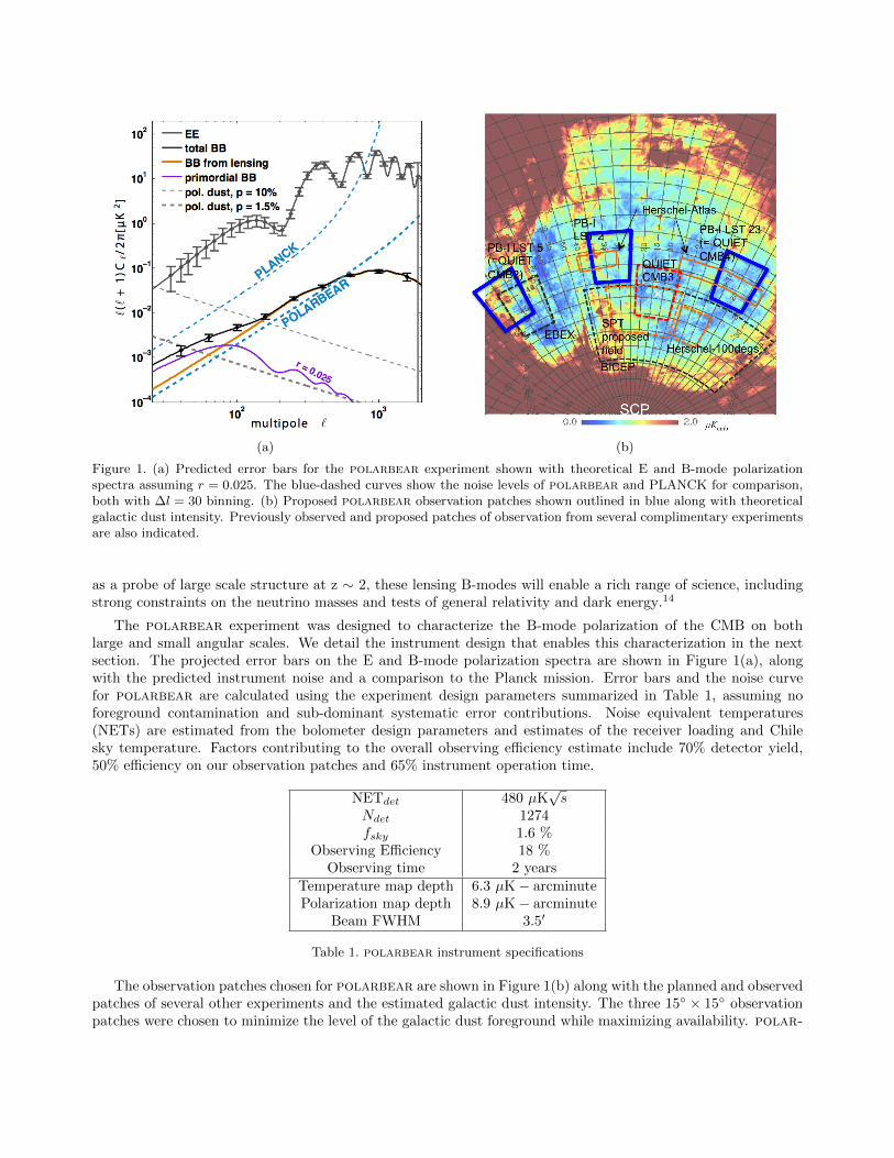
Figure 1. (a) Predicted error bars for the polarbear experiment shown with theoretical E and B-mode polarizationspectra assuming r = 0.025. The blue-dashed curves show the noise levels of polarbear and PLANCK for comparison,both with ∆l = 30 binning. (b) Proposed polarbear observation patches shown outlined in blue along with theoreticalgalactic dust intensity. Previously observed and proposed patches of observation from several complimentary experimentsare also indicated.

as a probe of large scale structure at z ∼ 2, these lensing B-modes will enable a rich range of science, includingstrong constraints on the neutrino masses and tests of general relativity and dark energy.14

The polarbear experiment was designed to characterize the B-mode polarization of the CMB on bothlarge and small angular scales. We detail the instrument design that enables this characterization in the nextsection. The projected error bars on the E and B-mode polarization spectra are shown in Figure 1(a), alongwith the predicted instrument noise and a comparison to the Planck mission. Error bars and the noise curvefor polarbear are calculated using the experiment design parameters summarized in Table 1, assuming noforeground contamination and sub-dominant systematic error contributions. Noise equivalent temperatures(NETs) are estimated from the bolometer design parameters and estimates of the receiver loading and Chilesky temperature. Factors contributing to the overall observing efficiency estimate include 70% detector yield,50% efficiency on our observation patches and 65% instrument operation time.

NETdet 480 µK√s

Ndet 1274fsky 1.6 %

Observing Efficiency 18 %Observing time 2 years

Temperature map depth 6.3 µK− arcminutePolarization map depth 8.9 µK− arcminute

Beam FWHM 3.5′

Table 1. polarbear instrument specifications

The observation patches chosen for polarbear are shown in Figure 1(b) along with the planned and observedpatches of several other experiments and the estimated galactic dust intensity. The three 15◦ × 15◦ observationpatches were chosen to minimize the level of the galactic dust foreground while maximizing availability. polar-

bear observes in a single spectral band centered at 148 GHz instrument. Overlap with the observation patchesof CMB experiments at other frequencies will enable foreground characterization and removal if required.

polarbear’s designed sensitivity and 3.5′ resolution will enable a greater than 10σ detection of the small-scaleB-mode signal due to gravitational lensing. When combined with data from the Planck satellite mission, datafrom polarbear will yield a 1σ error of 75 meV on the sum of the neutrino masses. Even when not combinedwith the larger sky coverage of Planck, polarbear will still provide a 1σ error of 150 meV independently. Onlarge angular scales, polarbear will enable a 2σ detection of r = 0.025. With this sensitivity, a significantmajority of large field slow-roll models of inflation can be either detected or ruled out.15

3. INSTRUMENT OVERVIEW

A measurement of the B-mode polarization requires significant new developments in receiver technology overprevious experiments. To characterize the B-mode polarization, the latest generation of millimeter wave receiversmust be designed with both sensitivity and systematic error control in mind. Since the B-mode signal is at leastan order of magnitude below the observed E-modes, even low levels of cross or instrumental polarization caneasily become sources of dominating systematic errors. The faint signal also requires careful attention to allaspects of experiment design, including desired instrument resolution and observation strategies.

State-of-the-art millimeter-wave detectors are limited only by the photon noise of the thermal background theyobserve. To increase overall sensitivity of the receiver and advance the instrument’s mapping speed, large arraysconsisting of thousands of such background-limited detectors that optimally sample a telescope’s throughput arebeing used. polarbear utilizes a unique 1,274 element lenslet coupled focal plane integrated with a large fieldof view telescope and cold reimaging optics to reach this goal. Low levels of systematic error contaminationare achieved with well-matched 3.5′ dual-polarized beams, an optical design with low sidelobe response, andseveral levels of baffling to mitigate ground pickup. Control and characterization of residual systematic errorsare achieved by employing a stepped half-wave plate along with a scan strategy that leverages sky-rotation toprovide polarization modulation.

3.1 The Huan Tran Telescope

The Huan Tran Telescope (HTT) is an off-axis Gregorian design that satisfies the Mizuguchi-Dragone condition.An advantage of off-axis telescopes is that they have clear apertures, lacking the secondary support structuresobstructing the beam that are required for on-axis telescopes. These structures can scatter or diffract signalfrom the ground into the main beam and severely limit performance. The Mizuguchi-Dragone condition setsthe tilt between the symmetry axes of the parent conics for the primary and secondary mirrors. The resultingantenna has a rotationally symmetric equivalent paraboloid, giving low cross polarization and astigmatism overa large diffraction-limited field of view.16,17 A Gregorian design has the advantage of a smaller secondary whencompared to the alternative crossed design and allows easier baffling to prevent far sidelobes due to scatteringat the receiver window. One disadvantage is that the Gregorian design suffers from a smaller diffraction-limitedfield of view than the equivalent crossed-dragone design.18

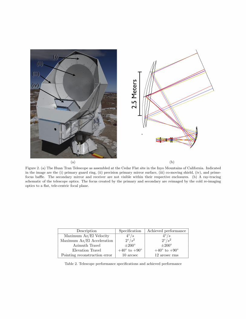
A ray-tracing schematic of the HTT’s optical design is shown in Figure 2(b). HTT has a 2.5 meter primarymirror that is precision machined from a single piece of aluminum to a 53 µm rms surface accuracy, alongwith a lower-precision guard ring that extends the primary paraboloid out to 3.5 meters in diameter. Highsurface accuracy and the monolithic design of the primary and secondary mirrors limit loss due to both diffusescattering19 and knife-edge diffraction in the case of segmented mirrors. The 2.5 meter primary gives a 3.5arcminute beam at 150 GHz, allowing the experiment to probe out to l ∼ 2500 and characterize the peak of thelensing B-mode spectrum at l ∼ 1000.

The telescope was built by VertexRSI∗ (now a part of General Dynamics). The specifications given to Vertexfor the telescope performance are summarized in Table 2 along with the performance we’ve currently achieved.A photo of the telescope fully assembled at the James Ax Observatory in Chile is shown in Figure 2(a)

(a)

2.5

Met

ers

(b)

Figure 2. (a) The Huan Tran Telescope as assembled at the Cedar Flat site in the Inyo Mountains of California. Indicatedin the image are the (i) primary guard ring, (ii) precision primary mirror surface, (iii) co-moving shield, (iv), and prime-focus baffle. The secondary mirror and receiver are not visible within their respective enclosures. (b) A ray-tracingschematic of the telescope optics. The focus created by the primary and secondary are reimaged by the cold re-imagingoptics to a flat, tele-centric focal plane.

Description Specification Achieved performanceMaximum Az/El Velocity 4◦/s 4◦/s

Maximum Az/El Acceleration 2◦/s2 2◦/s2

Azimuth Travel ±200◦ ±200◦

Elevation Travel +40◦ to +90◦ +40◦ to +90◦

Pointing reconstruction error 10 arcsec 12 arcsec rms

Table 2. Telescope performance specifications and achieved performance

Rotating HWP

Reimaging Lenses

Focal Plane

Pulse Tube Cooler

3 Stage HeSorption Fridge

Cold Aperture Stop

Window

SQUIDs

IR Blocking Filters

2.1 m

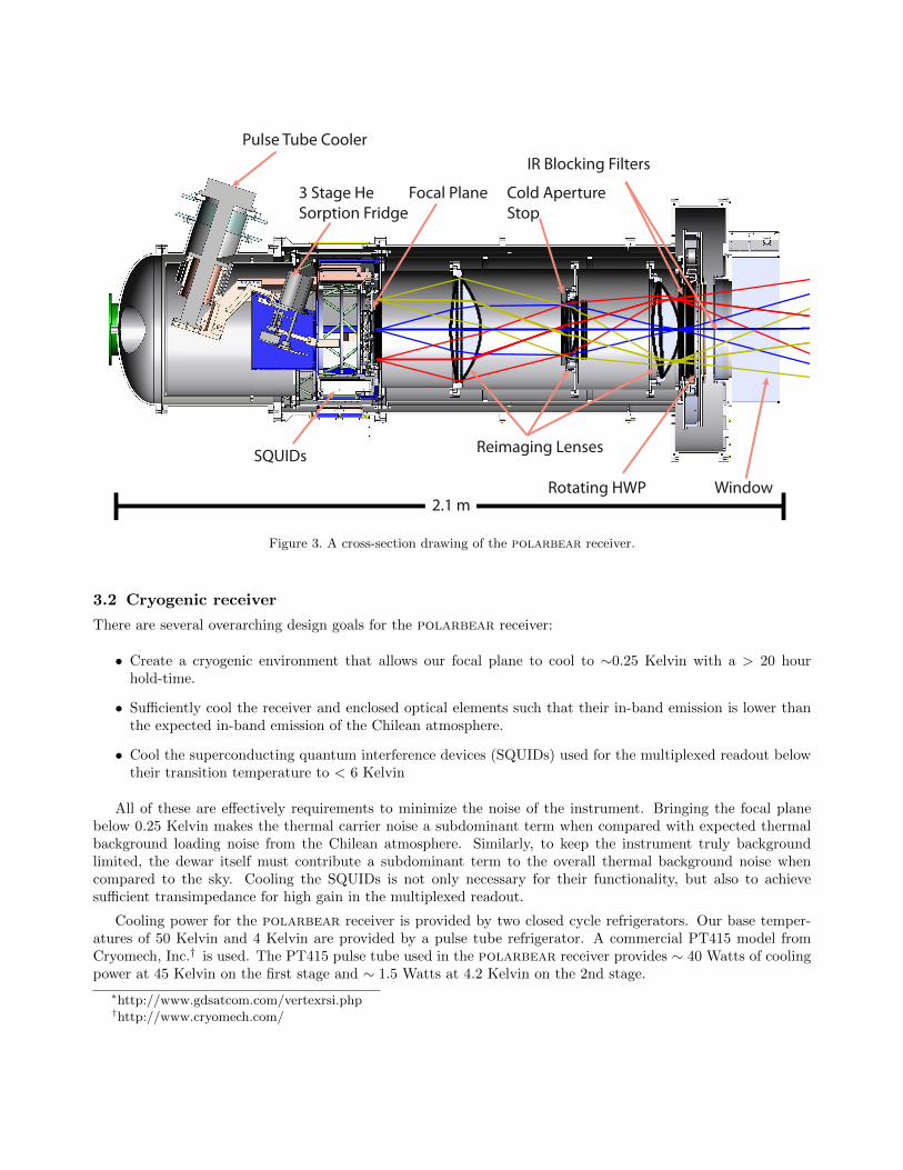
Figure 3. A cross-section drawing of the polarbear receiver.

3.2 Cryogenic receiver

There are several overarching design goals for the polarbear receiver:

• Create a cryogenic environment that allows our focal plane to cool to ∼0.25 Kelvin with a > 20 hourhold-time.

• Sufficiently cool the receiver and enclosed optical elements such that their in-band emission is lower thanthe expected in-band emission of the Chilean atmosphere.

• Cool the superconducting quantum interference devices (SQUIDs) used for the multiplexed readout belowtheir transition temperature to < 6 Kelvin

All of these are effectively requirements to minimize the noise of the instrument. Bringing the focal planebelow 0.25 Kelvin makes the thermal carrier noise a subdominant term when compared with expected thermalbackground loading noise from the Chilean atmosphere. Similarly, to keep the instrument truly backgroundlimited, the dewar itself must contribute a subdominant term to the overall thermal background noise whencompared to the sky. Cooling the SQUIDs is not only necessary for their functionality, but also to achievesufficient transimpedance for high gain in the multiplexed readout.

Cooling power for the polarbear receiver is provided by two closed cycle refrigerators. Our base temper-atures of 50 Kelvin and 4 Kelvin are provided by a pulse tube refrigerator. A commercial PT415 model fromCryomech, Inc.† is used. The PT415 pulse tube used in the polarbear receiver provides ∼ 40 Watts of coolingpower at 45 Kelvin on the first stage and ∼ 1.5 Watts at 4.2 Kelvin on the 2nd stage.

∗http://www.gdsatcom.com/vertexrsi.php†http://www.cryomech.com/

Subkelvin cooling is provided by a three stage, helium sorption fridge provided by Chase Research‡. Coolingpower is provided by pumping on condensed 4He and 3He in the various stages using charcoal pumps. Ourparticular fridge uses a sacrificial 4He cycle which condenses off the 4 K mainplate to provide a< 1 K condensationpoint for 3He used in the subsequent ‘ultrahead’ and ‘interhead’ stages. The interhead stage simply acts as abuffer to intercept thermal loads from wiring and structural members, allowing the ultrahead to reach ∼ 0.25K. Hold times of at least 24 hours are possible with loads of 80 µW on the interhead and up to 4 µW on theultrahead giving operating temperatures of 375 mK and 250 mK, respectively. Additional cooling power is alsoavailable at the heat exchanger, with ∼ 100 µW at an equilibrium temperature of ∼ 1.5 K.

The refrigerators can be seen in the receiver cross-section in Figure 3, along with various other componentsof the receiver. The main components to note are: the 30 cm Zotefoam window; IR blocking thermal filters; therotating half-wave plate, cooled to ∼80 Kelvin; reimaging lenses cooled to ∼6 Kelvin; the milliKelvin focal planeand the SQUID readout boards, cooled to ∼4 Kelvin. The cryogenic environment achieved allows the focal planeto cool to 250 milliKelvin with a resulting hold time greater than 30 hours.

3.2.1 Thermal filtering

A challenge to deploying large-format arrays is in developing cryogenic systems with sufficiently large aperturesfor the high optical throughput. The difficulty here is in rejecting radiation outside of the frequency band ofinterest to achieve a working cryogenic system while simultaneously mitigating in-band emission from the filterelements used. A receiver with cold, low in-band emissivity optical elements is required to assure that theinstrument sensitivity is limited by photon background loading from the sky rather than the receiver itself. Thistask is further complicated by the need to limit systematic effects that can be introduced by filtering elements.

This was addressed in polarbear with a filter stack consisting of several hot-pressed multilayer low-passfilters and single layer IR shaders,20,21 supplemented with an IR-absorbing 3 mm thick sheet of porous teflon.These filters, combined with the receiver’s Zotefoam vacuum window and cold re-imaging optics, mitigate theIR radiation incident on various cryogenic stages. The result is a cryogenic environment that meets our designgoals.

3.2.2 Polarization modulation

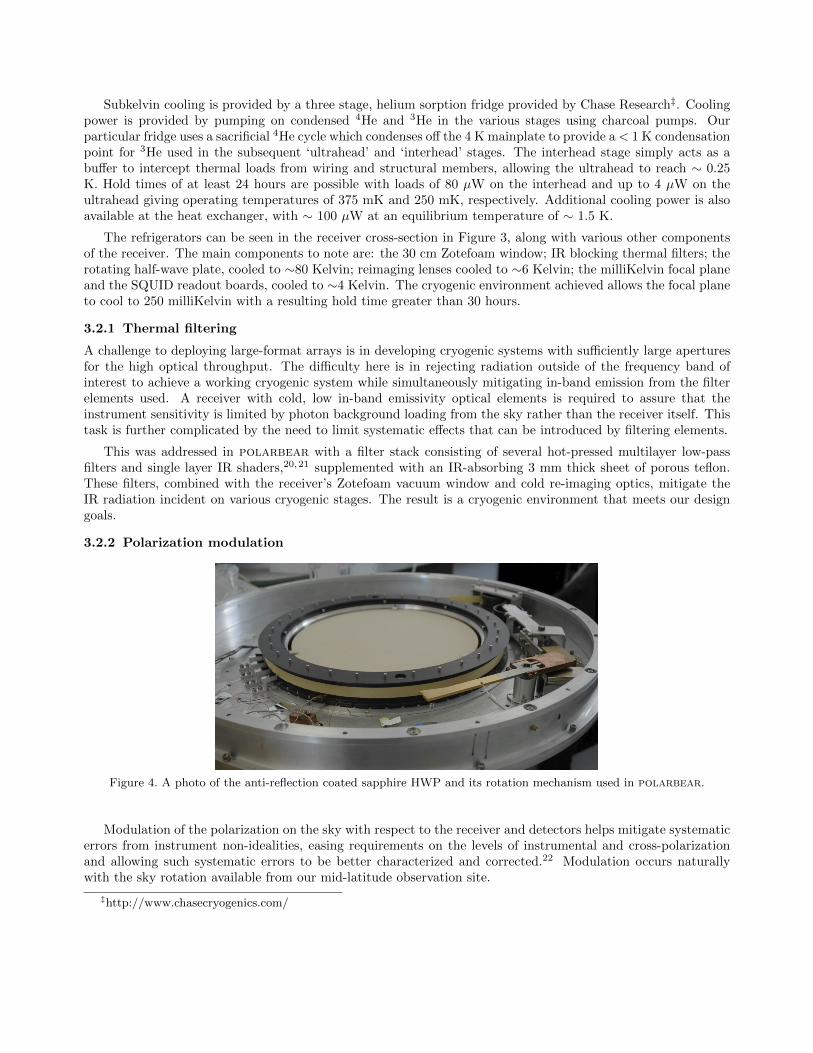
Figure 4. A photo of the anti-reflection coated sapphire HWP and its rotation mechanism used in polarbear.

Modulation of the polarization on the sky with respect to the receiver and detectors helps mitigate systematicerrors from instrument non-idealities, easing requirements on the levels of instrumental and cross-polarizationand allowing such systematic errors to be better characterized and corrected.22 Modulation occurs naturallywith the sky rotation available from our mid-latitude observation site.

‡http://www.chasecryogenics.com/

(a) (b)

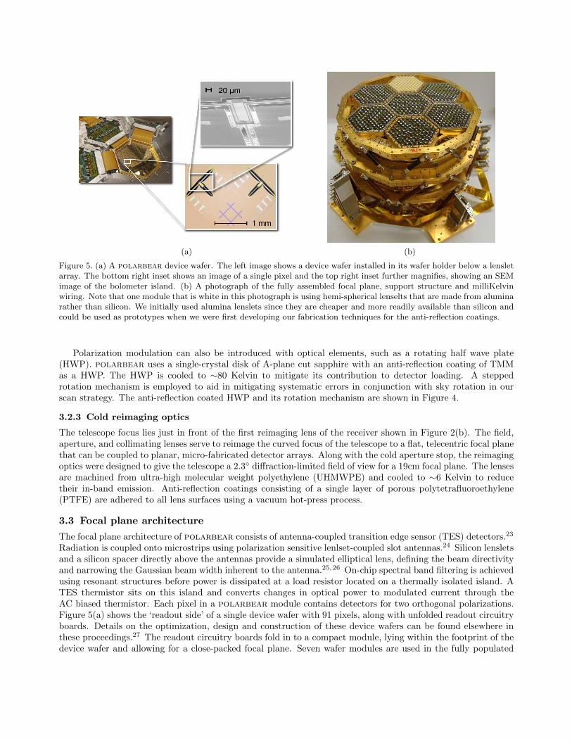
Figure 5. (a) A polarbear device wafer. The left image shows a device wafer installed in its wafer holder below a lensletarray. The bottom right inset shows an image of a single pixel and the top right inset further magnifies, showing an SEMimage of the bolometer island. (b) A photograph of the fully assembled focal plane, support structure and milliKelvinwiring. Note that one module that is white in this photograph is using hemi-spherical lenselts that are made from aluminarather than silicon. We initially used alumina lenslets since they are cheaper and more readily available than silicon andcould be used as prototypes when we were first developing our fabrication techniques for the anti-reflection coatings.

Polarization modulation can also be introduced with optical elements, such as a rotating half wave plate(HWP). polarbear uses a single-crystal disk of A-plane cut sapphire with an anti-reflection coating of TMMas a HWP. The HWP is cooled to ∼80 Kelvin to mitigate its contribution to detector loading. A steppedrotation mechanism is employed to aid in mitigating systematic errors in conjunction with sky rotation in ourscan strategy. The anti-reflection coated HWP and its rotation mechanism are shown in Figure 4.

3.2.3 Cold reimaging optics

The telescope focus lies just in front of the first reimaging lens of the receiver shown in Figure 2(b). The field,aperture, and collimating lenses serve to reimage the curved focus of the telescope to a flat, telecentric focal planethat can be coupled to planar, micro-fabricated detector arrays. Along with the cold aperture stop, the reimagingoptics were designed to give the telescope a 2.3◦ diffraction-limited field of view for a 19cm focal plane. The lensesare machined from ultra-high molecular weight polyethylene (UHMWPE) and cooled to ∼6 Kelvin to reducetheir in-band emission. Anti-reflection coatings consisting of a single layer of porous polytetrafluoroethylene(PTFE) are adhered to all lens surfaces using a vacuum hot-press process.

3.3 Focal plane architecture

The focal plane architecture of polarbear consists of antenna-coupled transition edge sensor (TES) detectors.23

Radiation is coupled onto microstrips using polarization sensitive lenlset-coupled slot antennas.24 Silicon lensletsand a silicon spacer directly above the antennas provide a simulated elliptical lens, defining the beam directivityand narrowing the Gaussian beam width inherent to the antenna.25,26 On-chip spectral band filtering is achievedusing resonant structures before power is dissipated at a load resistor located on a thermally isolated island. ATES thermistor sits on this island and converts changes in optical power to modulated current through theAC biased thermistor. Each pixel in a polarbear module contains detectors for two orthogonal polarizations.Figure 5(a) shows the ‘readout side’ of a single device wafer with 91 pixels, along with unfolded readout circuitryboards. Details on the optimization, design and construction of these device wafers can be found elsewhere inthese proceedings.27 The readout circuitry boards fold in to a compact module, lying within the footprint of thedevice wafer and allowing for a close-packed focal plane. Seven wafer modules are used in the fully populated

polarbear focal plane for a total of 1274 detectors paired in 637 pixels. The fully assembled focal plane insertdeployed to Chile is shown in Figure 5(b).

3.4 Multiplexing readout

A fundamental issue that one quickly runs into when developing a large detector array is in routing cryogenicwires. Bias signals must be sent from room temperature electronics down to cryogenic focal planes and readoutsignals must get back out without exceeding the cryogenic budgets of feasible milliKelvin refrigerators. Forarrays of TES bolometers, this has been addressed by several multiplexing technologies. Current through a lowimpedance, voltage-biased TES detector can be measured using a super-conducting quantum interference device(SQUID) by converting the current to magnetic flux with an inductor coil. For polarbear we use a frequencydomain multiplexer.28,29 The multiplexer allows many detectors to be biased with different AC bias frequencieson a single pair of wires and readout on another, using a single SQUID per multiplexed set. polarbear was oneof the first experiments deployed utilizing a newly developed digital frequency domain multiplexer (DfMux)30

with an 8× multiplexing factor.

4. STATUS AND PERFORMANCE

polarbear was first deployed on the HTT in 2010 at the Cedar Flat site of the CARMA array in the InyoMountains of California. The receiver was equipped with a subset of three of the seven planned detector arraysand only 1/3 of the readout for this engineering run. The entire instrument was integrated and underwent severalcharacterization tests. Among the characterization tests performed were intensity maps of bright sources forbeam characterization and telescope pointing evaluation and tests of polarization purity through measurementsof ground based and celestial sources. The successful engineering run help to refine the development of thereceiver and full focal plane in preparation for our science deployment to Chile. In late September of 2011,concrete was poured for the James Ax Observatory at an altitude of 5200 m on Cerro Toco in the Atacamadesert of Chile. In the 4 months that followed, the HTT was reassembled at the site and the polarbearreceiver integrated. First light with the fully integrated experiment was achieved on January 10th, 2012 with ascan of Jupiter. In this section, we present preliminary results on the instrument performance in Chile.

4.1 Beam maps

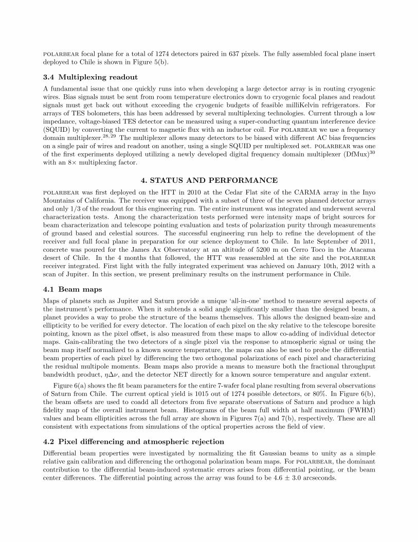
Maps of planets such as Jupiter and Saturn provide a unique ‘all-in-one’ method to measure several aspects ofthe instrument’s performance. When it subtends a solid angle significantly smaller than the designed beam, aplanet provides a way to probe the structure of the beams themselves. This allows the designed beam-size andellipticity to be verified for every detector. The location of each pixel on the sky relative to the telescope boresitepointing, known as the pixel offset, is also measured from these maps to allow co-adding of individual detectormaps. Gain-calibrating the two detectors of a single pixel via the response to atmospheric signal or using thebeam map itself normalized to a known source temperature, the maps can also be used to probe the differentialbeam properties of each pixel by differencing the two orthogonal polarizations of each pixel and characterizingthe residual multipole moments. Beam maps also provide a means to measure both the fractional throughputbandwidth product, η∆ν, and the detector NET directly for a known source temperature and angular extent.

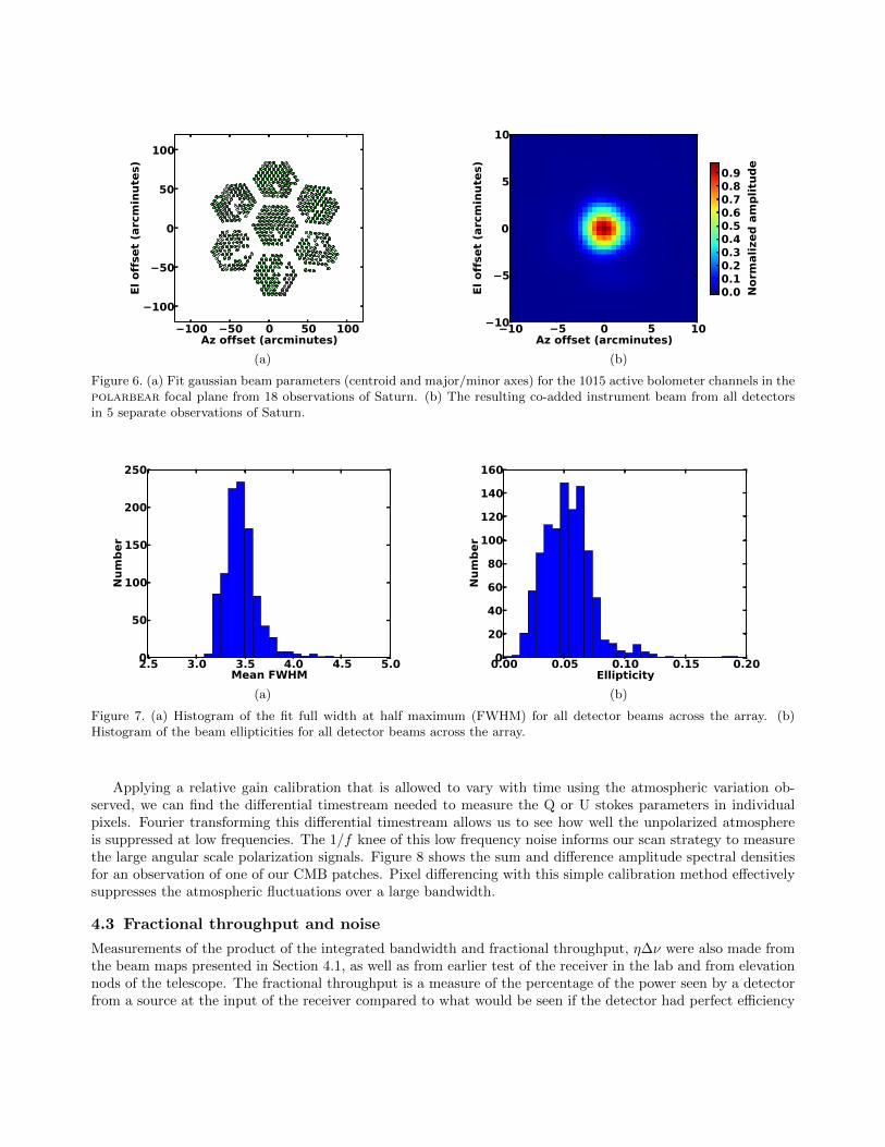
Figure 6(a) shows the fit beam parameters for the entire 7-wafer focal plane resulting from several observationsof Saturn from Chile. The current optical yield is 1015 out of 1274 possible detectors, or 80%. In Figure 6(b),the beam offsets are used to coadd all detectors from five separate observations of Saturn and produce a highfidelity map of the overall instrument beam. Histograms of the beam full width at half maximum (FWHM)values and beam ellipticities across the full array are shown in Figures 7(a) and 7(b), respectively. These are allconsistent with expectations from simulations of the optical properties across the field of view.

4.2 Pixel differencing and atmospheric rejection

Differential beam properties were investigated by normalizing the fit Gaussian beams to unity as a simplerelative gain calibration and differencing the orthogonal polarization beam maps. For polarbear, the dominantcontribution to the differential beam-induced systematic errors arises from differential pointing, or the beamcenter differences. The differential pointing across the array was found to be 4.6 ± 3.0 arcseconds.

100 50 0 50 100Az offset (arcminutes)

100

50

0

50

100El off

set

(arc

min

ute

s)

(a) (b)

Figure 6. (a) Fit gaussian beam parameters (centroid and major/minor axes) for the 1015 active bolometer channels in thepolarbear focal plane from 18 observations of Saturn. (b) The resulting co-added instrument beam from all detectorsin 5 separate observations of Saturn.

2.5 3.0 3.5 4.0 4.5 5.0Mean FWHM

0

50

100

150

200

250

Nu

mb

er

(a)

0.00 0.05 0.10 0.15 0.20Ellipticity

0

20

40

60

80

100

120

140

160N

um

ber

(b)

Figure 7. (a) Histogram of the fit full width at half maximum (FWHM) for all detector beams across the array. (b)Histogram of the beam ellipticities for all detector beams across the array.

Applying a relative gain calibration that is allowed to vary with time using the atmospheric variation ob-served, we can find the differential timestream needed to measure the Q or U stokes parameters in individualpixels. Fourier transforming this differential timestream allows us to see how well the unpolarized atmosphereis suppressed at low frequencies. The 1/f knee of this low frequency noise informs our scan strategy to measurethe large angular scale polarization signals. Figure 8 shows the sum and difference amplitude spectral densitiesfor an observation of one of our CMB patches. Pixel differencing with this simple calibration method effectivelysuppresses the atmospheric fluctuations over a large bandwidth.

4.3 Fractional throughput and noise

Measurements of the product of the integrated bandwidth and fractional throughput, η∆ν were also made fromthe beam maps presented in Section 4.1, as well as from earlier test of the receiver in the lab and from elevationnods of the telescope. The fractional throughput is a measure of the percentage of the power seen by a detectorfrom a source at the input of the receiver compared to what would be seen if the detector had perfect efficiency

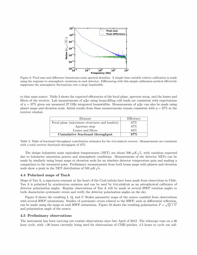
Figure 8. Pixel sum and difference timestream noise spectral densities. A simple time-variable relative calibration is madeusing the response to atmospheric variations in each detector. Differencing with this simple calibration method effectivelysuppresses the atmospheric fluctuations over a large bandwidth.

to that same source. Table 3 shows the expected efficiencies of the focal plane, aperture strop, and the lenses andfilters of the receiver. Lab measurements of η∆ν using beam-filling cold loads are consistent with expectationsof η = 37% given our measured 37 GHz integrated beamwidths. Measurements of η∆ν can also be made usingplanet maps and elevation nods. Initial results from these measurements remain consistent with η = 37% at thereceiver window.

Element Efficiency

Focal plane (microwave structures and lenslets) 67%Aperture stop 87%

Lenses and filters 64%

Cumulative fractional throughput 37%

Table 3. Table of fractional throughput contribution estimates for the polarbear receiver. Measurements are consistentwith a total receiver fractional throughput of 37%.

The design bolometer noise equivalent temperatures (NET) are about 500 µK√s, with variation expected

due to bolometer saturation powers and atmospheric conditions. Measurements of the detector NETs can bemade by similarly using beam maps or elevation nods for an absolute detector temperature gain and making acomparison to the measured noise. Preliminary measurements from both beam maps with planets and elevationnods show a peak in the NET distribution of 550 µK

√s.

4.4 Polarized maps of TauA

Maps of Tau A, a supernova remnant at the heart of the Crab nebula have been made from observtions in Chile.Tau A is polarized by synchrotron emission and can be used by polarbear as an astrophysical calibrator ofdetector polarization angles. Regular observations of Tau A will be made at several HWP rotation angles toboth characterize systematic errors and verify the detector polarization angles on the sky.

Figure 9 shows the resulting I, Q, and U Stokes parameter maps of the source coadded from observationswith several HWP orientations. Studies of systematic errors related to the HWP, such as differential reflection,can be made using the maps at each HWP orientation. Figure 10 shows the resulting polarization P =

√Q+ U

and polarization angle of the source.

4.5 Preliminary observations

The instrument has been carrying out routine observations since late April of 2012. The telescope runs on a 36hour cycle, with ∼20 hours currently being used for observations of CMB patches, 4.5 hours to cycle our mil-

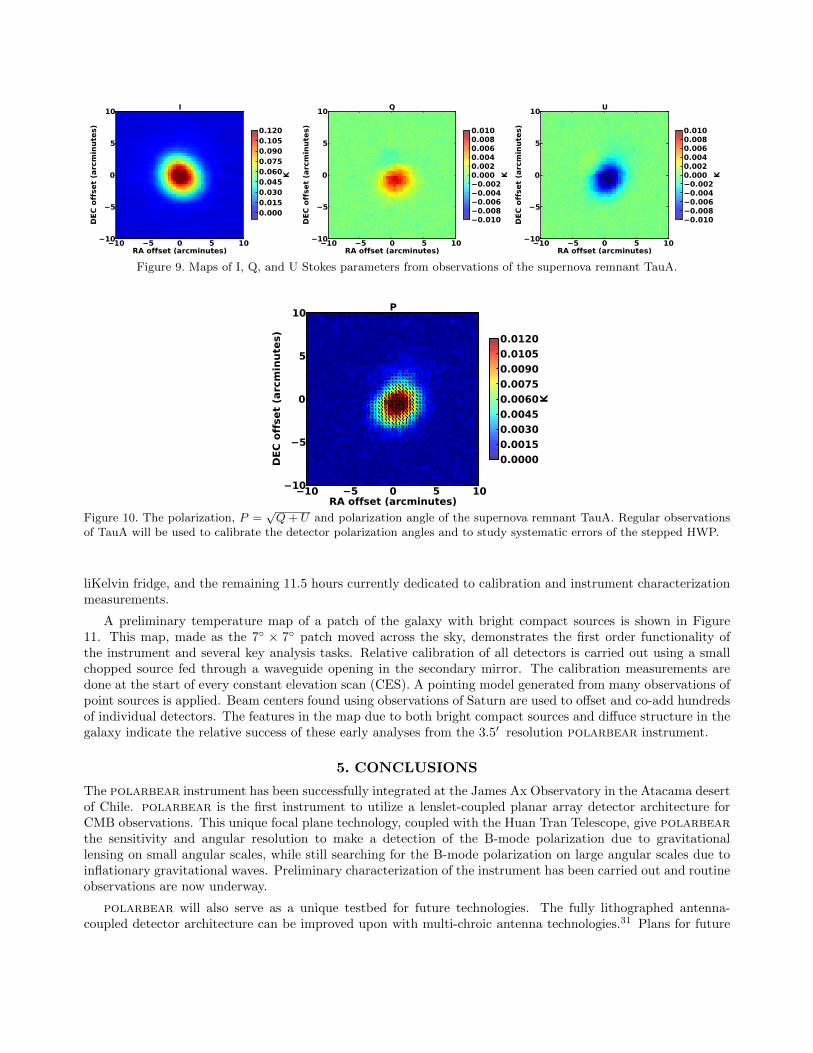
Figure 9. Maps of I, Q, and U Stokes parameters from observations of the supernova remnant TauA.

10 5 0 5 10RA offset (arcminutes)

10

5

0

5

10

DEC

off

set

(arc

min

ute

s)

P

0.0000

0.0015

0.0030

0.0045

0.0060

0.0075

0.0090

0.0105

0.0120

K

Figure 10. The polarization, P =√Q + U and polarization angle of the supernova remnant TauA. Regular observations

of TauA will be used to calibrate the detector polarization angles and to study systematic errors of the stepped HWP.

liKelvin fridge, and the remaining 11.5 hours currently dedicated to calibration and instrument characterizationmeasurements.

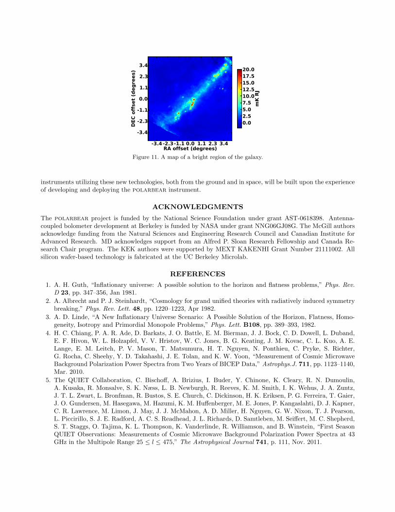
A preliminary temperature map of a patch of the galaxy with bright compact sources is shown in Figure11. This map, made as the 7◦ × 7◦ patch moved across the sky, demonstrates the first order functionality ofthe instrument and several key analysis tasks. Relative calibration of all detectors is carried out using a smallchopped source fed through a waveguide opening in the secondary mirror. The calibration measurements aredone at the start of every constant elevation scan (CES). A pointing model generated from many observations ofpoint sources is applied. Beam centers found using observations of Saturn are used to offset and co-add hundredsof individual detectors. The features in the map due to both bright compact sources and diffuce structure in thegalaxy indicate the relative success of these early analyses from the 3.5′ resolution polarbear instrument.

5. CONCLUSIONS

The polarbear instrument has been successfully integrated at the James Ax Observatory in the Atacama desertof Chile. polarbear is the first instrument to utilize a lenslet-coupled planar array detector architecture forCMB observations. This unique focal plane technology, coupled with the Huan Tran Telescope, give polarbearthe sensitivity and angular resolution to make a detection of the B-mode polarization due to gravitationallensing on small angular scales, while still searching for the B-mode polarization on large angular scales due toinflationary gravitational waves. Preliminary characterization of the instrument has been carried out and routineobservations are now underway.

polarbear will also serve as a unique testbed for future technologies. The fully lithographed antenna-coupled detector architecture can be improved upon with multi-chroic antenna technologies.31 Plans for future

-3.4-2.3-1.1 0.0 1.1 2.3 3.4RA offset (degrees)

-3.4

-2.3

-1.1

0.0

1.1

2.3

3.4

DEC

off

set

(deg

rees)

0.02.55.07.510.012.515.017.520.0

mK

RJ

Figure 11. A map of a bright region of the galaxy.

instruments utilizing these new technologies, both from the ground and in space, will be built upon the experienceof developing and deploying the polarbear instrument.

ACKNOWLEDGMENTS

The polarbear project is funded by the National Science Foundation under grant AST-0618398. Antenna-coupled bolometer development at Berkeley is funded by NASA under grant NNG06GJ08G. The McGill authorsacknowledge funding from the Natural Sciences and Engineering Research Council and Canadian Institute forAdvanced Research. MD acknowledges support from an Alfred P. Sloan Research Fellowship and Canada Re-search Chair program. The KEK authors were supported by MEXT KAKENHI Grant Number 21111002. Allsilicon wafer-based technology is fabricated at the UC Berkeley Microlab.

REFERENCES

1. A. H. Guth, “Inflationary universe: A possible solution to the horizon and flatness problems,” Phys. Rev.D 23, pp. 347–356, Jan 1981.

2. A. Albrecht and P. J. Steinhardt, “Cosmology for grand unified theories with radiatively induced symmetrybreaking,” Phys. Rev. Lett. 48, pp. 1220–1223, Apr 1982.

3. A. D. Linde, “A New Inflationary Universe Scenario: A Possible Solution of the Horizon, Flatness, Homo-geneity, Isotropy and Primordial Monopole Problems,” Phys. Lett. B108, pp. 389–393, 1982.

4. H. C. Chiang, P. A. R. Ade, D. Barkats, J. O. Battle, E. M. Bierman, J. J. Bock, C. D. Dowell, L. Duband,E. F. Hivon, W. L. Holzapfel, V. V. Hristov, W. C. Jones, B. G. Keating, J. M. Kovac, C. L. Kuo, A. E.Lange, E. M. Leitch, P. V. Mason, T. Matsumura, H. T. Nguyen, N. Ponthieu, C. Pryke, S. Richter,G. Rocha, C. Sheehy, Y. D. Takahashi, J. E. Tolan, and K. W. Yoon, “Measurement of Cosmic MicrowaveBackground Polarization Power Spectra from Two Years of BICEP Data,” Astrophys.J. 711, pp. 1123–1140,Mar. 2010.

5. The QUIET Collaboration, C. Bischoff, A. Brizius, I. Buder, Y. Chinone, K. Cleary, R. N. Dumoulin,A. Kusaka, R. Monsalve, S. K. Næss, L. B. Newburgh, R. Reeves, K. M. Smith, I. K. Wehus, J. A. Zuntz,J. T. L. Zwart, L. Bronfman, R. Bustos, S. E. Church, C. Dickinson, H. K. Eriksen, P. G. Ferreira, T. Gaier,J. O. Gundersen, M. Hasegawa, M. Hazumi, K. M. Huffenberger, M. E. Jones, P. Kangaslahti, D. J. Kapner,C. R. Lawrence, M. Limon, J. May, J. J. McMahon, A. D. Miller, H. Nguyen, G. W. Nixon, T. J. Pearson,L. Piccirillo, S. J. E. Radford, A. C. S. Readhead, J. L. Richards, D. Samtleben, M. Seiffert, M. C. Shepherd,S. T. Staggs, O. Tajima, K. L. Thompson, K. Vanderlinde, R. Williamson, and B. Winstein, “First SeasonQUIET Observations: Measurements of Cosmic Microwave Background Polarization Power Spectra at 43GHz in the Multipole Range 25 ≤ l ≤ 475,” The Astrophysical Journal 741, p. 111, Nov. 2011.

6. E. Komatsu, J. Dunkley, M. R. Nolta, C. L. Bennett, B. Gold, G. Hinshaw, N. Jarosik, D. Larson, M. Limon,L. Page, D. N. Spergel, M. Halpern, R. S. Hill, A. Kogut, S. S. Meyer, G. S. Tucker, J. L. Weiland,E. Wollack, and E. L. Wright, “Five-year wilkinson microwave anisotropy probe observations: Cosmologicalinterpretation,” The Astrophysical Journal Supplement 180, p. 330, Feb 2009.

7. M. Kamionkowski, A. Kosowsky, and A. Stebbins, “Statistics of cosmic microwave background polarization,”Phys. Rev. D 55, pp. 7368–7388, Jun 1997.

8. M. Zaldarriaga and U. Seljak, “All-sky analysis of polarization in the microwave background,” Phys. Rev.D 55, pp. 1830–1840, Feb 1997.

9. D. Baumann, M. G. Jackson, P. Adshead, A. Amblard, A. Ashoorioon, N. Bartolo, R. Bean, M. Beltran,F. de Bernardis, S. Bird, X. Chen, D. J. H. Chung, L. Colombo, A. Cooray, P. Creminelli, S. Dodelson,J. Dunkley, C. Dvorkin, R. Easther, F. Finelli, R. Flauger, M. Hertzberg, K. Jones-Smith, S. Kachru,K. Kadota, J. Khoury, W. H. Kinney, E. Komatsu, L. M. Krauss, J. Lesgourgues, A. Liddle, M. Liguori,E. Lim, A. Linde, S. Matarrese, H. Mathur, L. McAllister, A. Melchiorri, A. Nicolis, L. Pagano, H. V. Peiris,M. Peloso, L. Pogosian, E. Pierpaoli, A. Riotto, U. Seljak, L. Senatore, S. Shandera, E. Silverstein, T. Smith,P. Vaudrevange, L. Verde, B. Wandelt, D. Wands, S. Watson, M. Wyman, A. Yadav, W. Valkenburg, andM. Zaldarriaga, “Cmbpol mission concept study: Probing inflation with cmb polarization,” arXiv astro-ph/0811.3919v2, Nov 2008.

10. H. V. Peiris and R. Easther, “Recovering the inflationary potential and primordial power spectrum witha slow roll prior: methodology and application to wmap three year data,” Journal of Cosmology andAstroparticle Physics 07, p. 002, Jul 2006.

11. A. Lewis and A. Challinor, “Weak gravitational lensing of the cmb,” Physics Reports 429, p. 1, Jun 2006.

12. K. M. Smith, W. Hu, and M. Kaplinghat, “Weak lensing of the cmb: Sampling errors on b modes,” PhysicalReview D 70, p. 43002, Aug 2004.

13. L. Knox and Y.-S. Song, “Limit on the detectability of the energy scale of inflation,” Phys. Rev. Lett. 89,p. 11303, Jul 2002.

14. K. M. Smith, A. Cooray, S. Das, O. Dore, D. Hanson, C. Hirata, M. Kaplinghat, B. Keating, M. LoVerde,N. Miller, G. Rocha, M. Shimon, and O. Zahn, “Cmbpol mission concept study: Gravitational lensing,”arXiv astro-ph/0811.3916v1, Nov 2008.

15. L. Pagano, A. Cooray, A. Melchiorri, and M. Kamionkowski, “Red density perturbations and inflationarygravitational waves,” Journal of Cosmology and Astroparticle Physics 04, p. 009, Apr. 2008.

16. C. Dragone, “Offset multireflector antennas with perfect pattern symmetry and polarization discrimination,”ATT Tech. J. 57, p. 26632684, 1978.

17. M. A. Y. Mizugutch and H. Yokoi, “Offset dual reflector antenna,” IEEE International Symposium onAntennas and Propagation 14, p. 25, 1976.

18. H. Tran, A. Lee, S. Hanany, M. Milligan, and T. Renbarger, “Comparison of the crossed and the gregorianmizuguchi-dragone for wide-field millimeter-wave astronomy,” Applied Optics 47(2), pp. 103–109, 2008.

19. J. Ruze, “Antenna tolerance theory, a review,” Proceedings of the IEEE 54, pp. 633 – 640, april 1966.

20. P. Ade, G. Pisano, C. Tucker, and S. Weaver, “A review of metal mesh filters,” Proceedings of SPIE 6275,Jan 2006.

21. C. Tucker and P. Ade, “Thermal filtering for large aperture cryogenic detector arrays,” Proceedings ofSPIE 6275, Jan 2006.

22. M. Shimon, B. Keating, N. Ponthieu, and E. Hivon, “Cmb polarization systematics due to beam asymmetry:Impact on inflationary science,” Phys. Rev. D 77, p. 83003, Apr 2008.

23. M. J. Myers, W. Holzapfel, A. T. Lee, R. O’brient, P. L. Richards, H. T. Tran, P. Ade, G. Engargiola,A. Smith, and H. Spieler, “An antenna-coupled bolometer with an integrated microstrip bandpass filter,”Applied Physics Letters 86, p. 114103, Mar 2005.

24. G. Chattopadhyay and J. Zmuidzinas, “A dual-polarized slot antenna for millimeter waves,” Antennas andPropagation, IEEE Transactions on 46(5), pp. 736 – 737, 1998.

25. J. Zmuidzinas, N. Ugras, D. Miller, M. Gaidis, H. LeDuc, and J. Stern, “Low-noise slot antenna sis mixers,”Applied Superconductivity, IEEE Transactions on 5(2), pp. 3053 – 3056, 1995.

26. D. Filipovic, S. Gearhart, and G. Rebeiz, “Double-slot antennas on extended hemispherical and ellipticalsilicon dielectric lenses,” Microwave Theory and Techniques, IEEE Transactions on 41(10), pp. 1738–1749,1993.

27. K. Arnold, “The bolometric focal plane array of the polarbear cmb experiment,” These proceedings , 2012.

28. T. M. Lanting, H.-M. Cho, J. Clarke, W. L. Holzapfel, A. T. Lee, M. Lueker, P. L. Richards, M. A. Dobbs,H. Spieler, and A. Smith, “Frequency-domain multiplexed readout of transition-edge sensor arrays with asuperconducting quantum interference device,” Applied Physics Letters 86, p. 2511, Mar. 2005.

29. M. A. Dobbs, M. Lueker, K. A. Aird, A. N. Bender, B. A. Benson, L. E. Bleem, J. E. Carlstrom, C. L.Chang, H. M. Cho, J. Clarke, T. M. Crawford, A. T. Crites, D. I. Flanigan, T. de Haan, E. M. George, N. W.Halverson, W. L. Holzapfel, J. D. Hrubes, B. R. Johnson, J. Joseph, R. Keisler, J. Kennedy, Z. Kermish,T. M. Lanting, A. T. Lee, E. M. Leitch, D. Luong-Van, J. J. McMahon, J. Mehl, S. S. Meyer, T. E. Montroy,S. Padin, T. Plagge, C. Pryke, P. L. Richards, J. E. Ruhl, K. K. Schaffer, D. Schwan, E. Shirokoff, H. G.Spieler, Z. Staniszewski, A. A. Stark, K. Vanderlinde, J. D. Vieira, C. Vu, B. Westbrook, and R. Williamson,“Frequency Multiplexed SQUID Readout of Large Bolometer Arrays for Cosmic Microwave BackgroundMeasurements,” arXiv astro-ph.IM/1112.4215v1, pp. 1–26, Dec. 2011.

30. G. Smecher, F. Aubin, E. Bissonnette, M. Dobbs, P. Hyland, and K. MacDermid, “A Biasing and Demodu-lation System for Kilopixel TES Bolometer Arrays,” Instrumentation and Measurement, IEEE Transactionson 61(1), pp. 251–260, 2012.

31. A. Suzuki, “Multi-chroic dual-polarization bolometric detector for studies of the cosmic microwave back-ground,” These proceedings , 2012.