The inconsistency of French regulation mode faced with the

financialization of accumulation pattern

The contributions of Regulation approach and neo-Cambridgian modelling

Mickaël Clévenot1 and Yann Guy2

JEL : E12, E25, B15

Abstract: The absence of specifically dedicated method to represent financialized capitalism

constitutes a significant gap in contemporary macroeconomic modelling considering the im­

pact of finance on the rules of wealth production and distribution. From both the lessons of

Regulation theory in terms of accumulation pattern and regulation mode declined through

the concepts of institutional hierarchy and complementarity, and the neo-Cambridgian mod­

elling framework, one tries to establish the causes which prevail in the divergence of Americ­

an and French economies in the adoption of finance-led capitalism.

Keywords: modelling and macroeconomic simulation, institutional complementarity and hierarchy, accumulation regime, regulation pattern, financialization.

1 Researcher at the CEPN, University Paris-Nord Paris XIII, attached to the Maison des Sciences de l’Homme Paris Nord - 4 rue de la Croix Faron - 93210 Saint Denis la Plaine, e-mail: clevenot@seg.univ-paris13.fr.2 Ph.D. student at the GERME, University Paris-Diderot Paris VII - 103, rue de Tolbiac - Dalle des Olympiades - Immeuble Montréal - 75013 Paris, e-mail: yann.guy@orange.fr.

- 1 -

Financial liberalization undertaken from the end of the 1970s in the United States and in

Great Britain, has been followed in the current of the 1980s in a large majority of country. In

France, liberalization of the stock-accounts is accomplished in 1989. It had been preceded by

laws organizing national market liberalization since 1984. The impact of financial liberaliza­

tion remains ambiguous considering the diversity of the results. In Japan, it brings to mind

the deflationary crisis of the 1990s. In all the countries, it led to more or less pronounced

banking crisis (Ben Gamra & Clévenot [2005]). In the medium-term, the United States and

Great Britain experiment seems positive, whereas France suffers slow growth. It seems that

financial liberalization requires an institutional environment which is not present every­

where. In other words, the new institutional hierarchy imposed by finance does not spontan­

eously find the complementarities that are necessary to the flowering of a finance-led accu­

mulation pattern. One will try to determine these conditions thanks to models of closed eco­

nomies.

Standard models fail to apprehend correctly formal treatment of accumulation pattern con­

trolled by stock effects. The Neoclassical-Keynesian synthesis models produce many incon­

sistencies in analysis of the currency and of the financial titles, particularly in the stock-flow

relations, because of the absence of accounting consistency and stock effects, which are

however implicit in the definition of flows equilibrium links (Taylor [2004a, 2004b]). In

neo-classical models with rational expectations, there is no differences between flows and

stocks at the equilibrium, namely an flow or stock equilibrium is defined, but not there is no

interactions between them (Foley [1975]).

The regulation theory teaches that transition from fordian regime to patrimonial regime ex­

presses both an inversion of the institutional hierarchy and the formation of new comple­

mentarities. However, formal representation of financialized capitalism established by Regu­

lationnists authors is also not satisfactory enough. Thus, in this article, one tries to model

these relations thanks to neo-Cambridgian macroeconomic models. From the initial model

sets up by Godley and Lavoie (2001), one modifies the locking-up variables in income distri­

bution as well as the behaviour equations in order to represent institutional inversion phe­

nomena. Firm’s stockholding behaviour is studied from now on. The model is then outlined

in three versions, in order to establish the installation requirements of a new coherence con­

fronting the new political deal, the increase in power of finance and the weakening of work­

ers power.

- 2 -

Section 1 Representations of finance-led capitalism

1.1. Theoretical presentation of financialized capitalism

Aglietta (1998) is the first economist in France who tries to provide a comprehensive repres­

entation of the financialized capitalism, named patrimonial capitalism. The Regulationnist

author has advanced the notion of a mode of accumulation based on finance to explain the

American performances. The reconfiguration of capitalism would be carried out from an in­

version of the fordian institutional hierarchy. The wage labour nexus then dominating would

become a variable subordinate to the constraints imposed by monetary regime and finance,

which constituted the adjustment variables of the former period. Performances of the patri­

monial ¨regime would be explained by the adequacy of the mode of regulation to accumula­

tion pattern.

This idea caused many reactions insofar as the existence of an accumulation pattern implies

its diffusion in other economies, including in France. This exportation of the American re­

gime supposes, in theory, a major questioning of social relations which prevail in France

since the post-war period, since it implies a substantial modification of the system of social

protection. From this perspective, the question of existence of the patrimonial accumulation

pattern in the United States has important implications for the French political economy.

The weakness of the hexagonal economy during a broad part of the 1990s could thereby be

explained by the lateness in new working rules adoption for finance-dominated economy

(Aglietta [2000]).

In order to look into this considering, Regulationnists authors implemented several model­

ling. But the formalization of a financialized accumulation pattern whose United States of

years 1990/2000 was supposed to be an archetype (Aglietta [1998]) is realized with a too

partial description of the wealth effects (Boyer [2000]). If the financial aspects are more pre­

cisely handled, it is the macroeconomic closing which is lacking (Aglietta & Breton [2001],

Aglietta & Rebérioux [2004]). However, financialization effects require special attention.

This dissatisfaction leads up to fall back on formalizations borrowed from the neo-Cam­

bridgian approach developed by Godley and Lavoie (2001). One amends them and extends

their analysis field. Even if it is not its first purpose, this approach known as “Stock Flow

Consistent Approach to macroeconomic modelling” (SFCA), seems able to meet require­

ments of a macroeconomic analysis that fully takes into consideration the financial interac­

tions. The modifications concerned some behavioural equations but especially modifications

in the distributive aspects in order to reveal hierarchy and institutional complementarity

- 3 -

phenomena. The field of analysis was extended to more financial aspects as increase in secur­

ities issuing, increase in households, increase in shareholder pressure or share buybacks by

firms while preserving the more traditional aspects of economic policy.

1.2. Formalization of the institutional hierarchy and complementarity

The fordian crisis, which starts in the late of the 1960s, gave rise to significant economic, in­

stitutional and political modifications. The transformations of accumulation pattern led to a

structural crisis because of the inadequacy of the regulation mode. During the crisis, all in­

stitutions are affected: form of state interventions, form of competition, international regime,

monetary system and wage relation. The modelling efforts will focus on these two last insti­

tutions. The modelling is limited with a closed economy, so that the globalisation implica­

tions cannot completely be dealt with.

The monetary system knew very important evolutions on the two sides of the Atlantic. Since

1979, policies against inflations and the abandonment of the fixed exchange rate regime

(1971) support the transition from indebtedness regime to stock market regime, generating

an inversion of the institutional hierarchy. Inflation revealed social conflict between capital

and labour. Employment constitutes from now on the adjustment variable, instead of the

monetary policy. The rise of unemployment in the last 1970s and during the 1980s estab­

lishes an unfavourable situation for the wage interest.

With the sustained and non-inflationary high growth in the United-States during the 1990s,

it was reasonable to think that this country came out of the fordian crisis, in other words that

the mode of regulation was adapted to new accumulation pattern. This new social and policy

configuration during the 1990s appears to explain a new lease on life in the United States

while it seems rather negative in France. Within the framework of this work, one will strive

to explain this divergence.

The basic assumption consists in supposing that the accumulation pattern in France and in

the United States imposed by finance has the same attributes and that the difference between

the two economies depends on the mode of regulation. The difficulty is then in the way of

formalizing the social power struggle, because institution hierarchy follows from this power

struggle.

The social conflict is worked by former institutions and social history of the political eco­

nomies in which it occurs. Thus, the modification of institutions is both an expression and a

limit to this capacity of transformation. Their representation can help to understand the is­

sues of the conflict, and possibly the ways in which could be established a new status quo. In

- 4 -

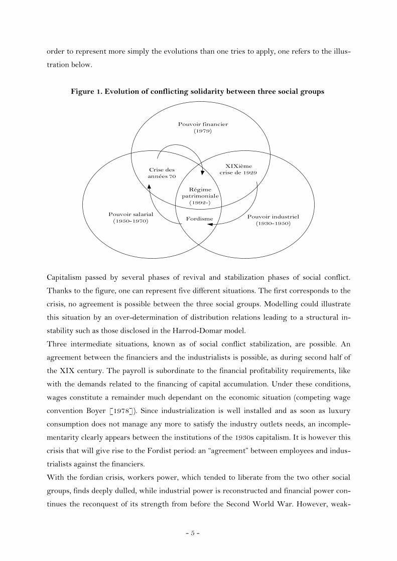
order to represent more simply the evolutions than one tries to apply, one refers to the illus­

tration below.

Figure 1. Evolution of conflicting solidarity between three social groups

Pouvoir financier(1979)

Pouvoir salarial(1950-1970)

Pouvoir industriel(1930-1950)

Fordisme

XIXième crise de 1929

Régime patrimoniale

(1992-)

Crise des années 70

Capitalism passed by several phases of revival and stabilization phases of social conflict.

Thanks to the figure, one can represent five different situations. The first corresponds to the

crisis, no agreement is possible between the three social groups. Modelling could illustrate

this situation by an over-determination of distribution relations leading to a structural in­

stability such as those disclosed in the Harrod-Domar model.

Three intermediate situations, known as of social conflict stabilization, are possible. An

agreement between the financiers and the industrialists is possible, as during second half of

the XIX century. The payroll is subordinate to the financial profitability requirements, like

with the demands related to the financing of capital accumulation. Under these conditions,

wages constitute a remainder much dependant on the economic situation (competing wage

convention Boyer [1978]). Since industrialization is well installed and as soon as luxury

consumption does not manage any more to satisfy the industry outlets needs, an incomple­

mentarity clearly appears between the institutions of the 1930s capitalism. It is however this

crisis that will give rise to the Fordist period: an “agreement” between employees and indus­

trialists against the financiers.

With the fordian crisis, workers power, which tended to liberate from the two other social

groups, finds deeply dulled, while industrial power is reconstructed and financial power con­

tinues the reconquest of its strength from before the Second World War. However, weak­

- 5 -

ness of the wage incomes penalizes total dynamics through consumption. To cancel this risk

weighing on the viability of an accumulation pattern, it is necessary to define allowances that

will allow wage-related demand to be maintained to a satisfactory level. Indebtedness and

price-cutting of capital goods as part of mondialized economy, are involved in the purchasing

power maintenance. Nevertheless, within the framework of the model where households can­

not get into debt and where one is in a closed economy, only financial incomes can offset

weak wages. This situation corresponds to the theoretical framework of patrimonial capital­

ism. From a social point of view, this configuration constitutes a singular situation in which

a balance between the three social groups could appear.

This situation would be made possible because of weak workers power, enabling reforms that

validate by institutions the position of workers power like wage flexibilization of the wage

labour nexus and liberal management of social protection. These modifications make it pos­

sible to increase long-run saving which increases firms’ capital stock and reinforce the pro­

ductive discipline through market vigilance and hostile operations. The financiers organize

these transformations for the benefit of financial capital holders among which one should

find an increasingly significant part of employees. From a macroeconomic point of view, the

reduction of wages is offset by allowances of financial origin.

The differentiation of the configurations is justified by the concepts that theoretically base

the consistency of finance-led regime: institutional hierarchy and complementarity. The in­

stitutional hierarchy is represented by the methods of income distributions, while the com­

plementarities are transcribed in the consumption function. The variable that carries the

closing of the distribution identifies the social group in a weak position. The group whose in­

comes are established like a fixed share of the GDP, net profit or investment determines de­

grees in social hierarchy. It is thus possible to determine the balance of power between the

three actors of the models: households, firms and shareholders. These various rules of in­

come distribution, incorporated in a specific institutional framework, allow making emerge

more or less coherent situations, according to the determination rules of the consumption

level. The most coherent financialized regime is represented by a weak workers power, an in­

termediate situation for the industrial power and a dominant position for the financiers. In

this configuration, wages are less important but the financial incomes are higher. Also,

propensities to spend wage incomes and financial incomes must change so that the rise of fin­

ancial incomes compensates fall in wages in the definition of the consumption level. In the

case of a wage reduction imposed by an increase in dividends, consumption and growth can

be maintained whereas in a more Fordist regime where demand remains largely defined by

wage incomes, consumption and growth should be weakened. The institutional inconsisten­

- 6 -

cies would thus contribute to explain divergences concerning the evolution of the French

and American economies face with rise of finance. In all configurations, one retains a com­

plete subordination of wages. They constitute a remainder. Profits should take this form in a

traditional idea of the economy functioning. In the following section, we will reconsider

more precisely these questions.

Section 2. Presentation of the model

The section begins with the presentation of the model accounting framework then models

are presented through theirs equations and their diverse closures.

1. The social accounting framework

The model represents a closed economy, made up of 31 equations. Three agents are presents:

households, companies and banks. The households have three types of earnings, wages (Wd),

dividends (Fdm) and interest paid by the banks which remunerates theirs deposits (rm*Md

(-1)). Companies receive the proceeds from their production (GDP), plus the dividends that

they perceive of their stockholding (Fde). Companies can buy back part of their owns equit­

ies. The interest of such a transaction lies in the possibility of exploring the consequences of

equity repurchase policy such as they were implemented in the United States 3 and more re­

cently in France. Saving of the companies, or retained profit (Fu), increase in debt (∆Ls) and

new issues of securities (pe*∆es) are the resources that ensure the financing of productive

and financial capital. Banks perceive the debtor interests paid by companies (rl*Ld(-1)). They

lend money with household deposits (∆Ms). Households could use their incomes in three

ways: consumption (Cd), deposits (∆Md), and equities (∆Edm* Pe).

3 In the United States, the net equity issues have been negative since the middle of the Nineties. The argument according to which liberalization would make it possible to reduce costs of financing is thus called into ques­tion. This flaw makes it possible to underline a second aspect of financial liberalization; the capacity to operate quick capital restructuring. It is this element which constitutes the central point of contemporary financial lo­gic: financial capital liquidity.

- 7 -

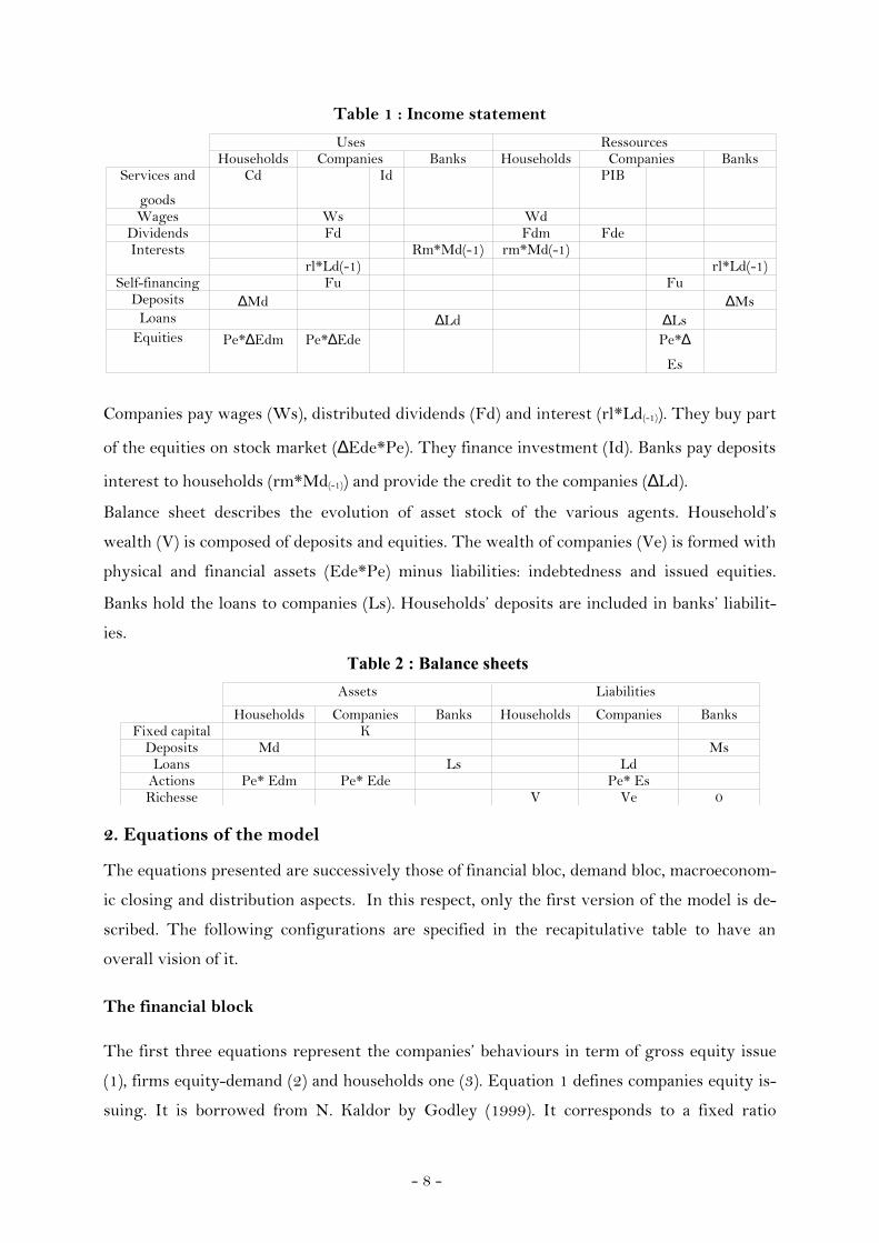
Table 1 : Income statement

Uses RessourcesHouseholds Companies Banks Households Companies Banks

Services and

goods

Cd Id PIB

Wages Ws WdDividends Fd Fdm FdeInterests Rm*Md(-1) rm*Md(-1)

rl*Ld(-1) rl*Ld(-1)Self-financing Fu Fu

Deposits ∆Md ∆MsLoans ∆Ld ∆Ls

Equities Pe*∆Edm Pe*∆Ede Pe*∆

Es

Companies pay wages (Ws), distributed dividends (Fd) and interest (rl*Ld(-1)). They buy part

of the equities on stock market (∆Ede*Pe). They finance investment (Id). Banks pay deposits

interest to households (rm*Md(-1)) and provide the credit to the companies (∆Ld).

Balance sheet describes the evolution of asset stock of the various agents. Household’s

wealth (V) is composed of deposits and equities. The wealth of companies (Ve) is formed with

physical and financial assets (Ede*Pe) minus liabilities: indebtedness and issued equities.

Banks hold the loans to companies (Ls). Households’ deposits are included in banks’ liabilit­

ies.

Table 2 : Balance sheets Assets Liabilities

Households Companies Banks Households Companies BanksFixed capital K

Deposits Md MsLoans Ls Ld

Actions Pe* Edm Pe* Ede Pe* EsRichesse V Ve 0

2. Equations of the model

The equations presented are successively those of financial bloc, demand bloc, macroeconom­

ic closing and distribution aspects. In this respect, only the first version of the model is de­

scribed. The following configurations are specified in the recapitulative table to have an

overall vision of it.

The financial block

The first three equations represent the companies’ behaviours in term of gross equity issue

(1), firms equity-demand (2) and households one (3). Equation 1 defines companies equity is­

suing. It is borrowed from N. Kaldor by Godley (1999). It corresponds to a fixed ratio

- 8 -

between investment and equity issuing. This simple formalization is abandoned. The writing

which one retains, takes as a starting point the econometrics results established for France

(Clévenot, Guy & Mazier [2007]). It indicates the presence of a positive effect between the

possibilities of firms indebtedness refunding and the equity issuing ( 1τ >0), as well as a posit­

ive elasticity regarding debtor interest rate indicating a logical phenomenon of arbitration

between the various sources of financing ( 2τ >0).

(1)( )-1

1 2 0ΔEs * pe L = * + * rl +

I Fu τ τ τ

Companies stockholding behaviour is also inspired by the econometric results obtained for

France. One defines the variation of desired quantities of equities on the total assets of com­

panies by a positive relation with the profitability of the previous equities held ((τ1 *ree(-1))

and a positive relation with the return on investments ((τ2*rcf), which represents a capacity of

financing.

(2) ( )( ) ( ) ( )1 -1 2 -1 0Ede * pe = * ree + * rcf +

Ede * pe + Kη η η∆

Households’ demand for equities is made according to portfolio behaviour a la Tobin. It al­

lows defining equity price. One supposes a negative relationship with the deposits profitabil­

ity (ψ1<0), a positive elasticity regarding return on equity previously held by households (ψ

2>0) and a negative effect, related to a demand for liquidity (ψ3 < 0)

(3)* *

1 2 3 0*

pe*Edm Yhr = * rm + * rem(-1) + * + V V

ψ ψ ψ ψ

The three following accounting equations allow to endogeneize the overall equity demand

(Ed) which corresponds to the demand of households (Edm) and companies (Ede). The net

equity supply of the companies (Ese) is obtained by subtracting from gross equity issuing

(Es), the companies demand (Ede). Lastly, the households demand is logically equivalent to

the net supply of firms (6).

(4) Ed = Edm + Ede

(5) Ese = Es - Ede

(6) Edm = Ese

Variation of the households’ deposits (∆Md) is determined by an accounting equation. It

means that deposits correspond to a balance between the different household incomes. Vari­

- 9 -

ation of households wealth (∆V) corresponds to an increase in saving, i.e. incomes not con­

sumed, at which it is necessary to withdraw the uses related to financial accumulation (∆

Edm*pe) which reduce households cash, and capital gains which are already considered in

the evolution of wealth (∆pe*Edm(-1)).

(7) (-1)Md = V - pe * Edm - Edm * pe∆ ∆ ∆ ∆

Companies debt (∆Ld) also corresponds to a “buffer”, namely an adjustment variable which,

if necessary, allows companies to fill in the weakness of their financing sources for invest­

ment if self-financing (Fu) and new net equity issue are not enough (∆Ese*pe). Accounting

framework is fixed so that the amount of money supplied by households, through the inter­

mediary of banks, corresponds exactly to the needs of companies, without writing explicit

equation of this equality (L=M) which rises from the accounting balance of the model and

which can be checked at the time of simulations.

(8) Ld = I - Fu - Edm * pe-Fde∆ ∆ 4

The amount of deposits anticipated by households ( )*Md fits with the difference between

their level of expected wealth ( )*V and the amount of their financial saving (Edm*pe).

(9) ( )* *Md = V - Edm * pe

Debtor interest rate is equal to credit interest rate so as to avoid the appearance of banking

profits which would complicate the model. The debtor rate is exogenous.

(10) rm = rl

The two following equations represent the capital gains realized respectively by households

and companies.

(11) (-1)CGm = pe * Edm∆

(12) (-1)CGe = pe * Ede∆

4 Equation 8 should be written as follows: Ld = I - Fu - Ese * pe∆ ∆ -Fde, the needs for external finan­cing are represented by the difference between level of investment minus self-financing and net issuing of firms. However, one writes it by using the net equity purchases of households, what is equivalent from an accounting point of view, but reduced the difference with initial values because of calibrations difficulties, so that the equal­ity Ld = Md is immediately observed, allowing to validate the accounting consistency of the model. Otherwise, convergence is underlying and not instantaneous. In order to correct this calibration problem, one chooses this option.

- 10 -

Equations (13) and (14) establish the amount of dividends perceived by households and com­

panies which corresponds respectively to the share of equities held by households and com­

panies. (13)EdmFdm = Fd *Es

(14)EdeFde = Fd *Es

Equations (15) and (16) establish the rate of profitability of the equities held by households

(rem) and by companies (ree).

(15)( )

( )(-1) (-1)

Fde + CGeree =

pe * Ede

(16)( )

( )(-1)

Fdm + CGmrem =

pe(-1) * Edm

Evolution of effective wealth (∆V) results from households saving, at which are added capital

gains. Expected wealth level corresponds to the previous wealth level at which household

saving is incorporated, namely expected incomes less consumption plus capital gains.

(17) V = Yhr - Cons + CGm∆

(18) * *(-1)V = V + Yhr + CGm - Cons

The demand block

Two specifications are retained to define consumption. In the first two patterns, it is identical

(19.1 and 19.2). Household consumption is related to two propensities, which one to consume

expected incomes ( )*1 * Yhrα and which one to consume wealth ( )3 (-1) * Vα .

(19.1) *0 1 2 (-1)Cons = + * Yhr + * Vα α α

In the last pattern, to reveal the institutional complementarity necessary to the consistency

of finance-led regime induced by the modification of institutional hierarchy, one reduces

propensity to consume out of incomes (α1 = 0.8, α11 = 0.7). Propensity to consume out of di­

vidends and wealth do not change (α12 = 0.8, α2 = 0.05). On the other hand, one reduces

propensity to consume out of monetary incomes (α13 = 0.5) in order to reduce the effect of

activity rise induced by the increase in monetary incomes after the rise of interest rates.

- 11 -

(19.3) 0 11 (-1) 12 (-1) 13 (-1) 2 (-1)Cons = + *W + * Fd + *rl*L + * Vα α α α α

The regular income follows the Haig-Simon definition retained by Godley. It corresponds to

the addition of the resources drawn from dividends as well as the interests received by

households from their deposit.

(20) (-1)Yhr = W + Fdm + rm * M

Expectations are very rough compared to model with microeconomics foundations but it is

about a theoretical choice meaning that at agglomerate level, there are regularities between

various ratios. Expected income arises like the projection of past incomes multiplied by the

effective growth rate of previous income.

(21)(-1)

Yhr gy = Yhr∆

(22) *(-1) (-1)Yhr = (1 + gy ) * Yhr

The rate of capital accumulation determines the demand for investment from companies.

This equation retains an acceleration effect by demand (φ3 = 0.015) and financials variables,

elasticity regarding rate of profit ( )1 = 0.5φ , elasticity regarding indebtedness ratio

( )2 = 0.25φ as well as a positive constant ( 0 φ > 0).

(23) ( ) (-1)1 -1 2 3 0

(-1) (-1)

LΔPIBg = * rcf - * + * + K PIB

φ φ φ φ

Investment level rises from the rate of accumulation applied to capital stock of capital, at pre­

vious period.

(24) (-1)I = g * K

(25) (-1)K = K * (1 - + g)δ

Macroeconomic closure and distribution aspects

Distribution aspects are essential in the modelling of the inversion of institutional hierarchy.

Also, two equations are modified according to configurations, gross profit equation (28.3),

and retained profits equation (29). The equation defining dividends does not evolve but the

relationship between industrialists and financiers is modified through the equation of self-fin­

ancing (29). The equation of wages is endogeneized, what underlines the wages subordina­

tion in incomes distribution.

- 12 -

GDP corresponds to the sum of firms’ investment and households’ consumption. (26)

PIB = Cons + I

Wages in this series of model are defined as would be profits, in the form of a remainder.

They are established by balance between GDP and profits. This representation allows estab­

lishing wages like hierarchically inferior to self-financing (industrial power) and dividends

(financial power).

(27) W = PIB Ft−

The determination of self-financing and gross profits equations thus will makes it possible to

fix the dominant social group of the model. In first and last configurations, profits are

defined in an accounting way as the sum of self-financing, dividends and debt burden. In the

second they are established like a proportion of the GDP. They are defined like wages ( 1ι

=0.33).

(28.1) Ft = Fu + Fd + rl * L(-1)

(28.2) 1Ft = * PIB - W0ι

(28.3) Ft = Fu + Fd + rl * L(-1)

The distribution of dividends is proportional to the gross profits level after debt repayment.

The rule of dividends distribution is represented by (1-sf). This writing underlines the pres­

sure exerted by shareholders.

(29) ( ) ( )(-1)Fd = 1 - sf * Ft - rl * L

The self-financing in the first configuration is proportional to the investment observed in the

previous period ( 1ϑ = 0.33). In the second, it is established like a remainder on the basis of

gross profits, at which one withdraws dividends and debt burden. In the last one, it is defined

like wages by a proportion of GDP ( 1υ =0.1).

(30.1) 1 Fu = * I(-1) - W0ϑ

(30.2) Fu = Ft - Fd - rl * L(-1)

(30.3) 1 (-1) Fu = * PIB - W0υ

Finally, one can establish the rate of profit like a ratio of profit over capital stock.

(31) (-1)

Furcf = K

The combination of these various methods of income distribution of income is supposed to

allow defining the power of various social groups. Employees are the most weak. It remains

to establish the relative position of industrialists and financiers.

- 13 -

In the first case, self-financing is imposed by industrialists as a fixed proportion of invest­

ment. Their situation is intermediate, they preserve a space decision but they don’t enjoy

growth directly. Gross profit, defined in an accounting-way, transfers to employees the re­

quirements of income distribution closure. In the second case, gross profit is proportionally

defined to GDP, what could lead to believe that industrials are dominants but self-financing

is defined as a remainder. Industrials power is thus limited. The financial ones are dominant

in this configuration. The importance of gross profits contributes to the reinforcement of

paid dividends. In the last case, power is better distributed between industrialists and finan­

ciers since retained profit is directly fixed on GDP, industrialists take advantage of growth

for investment financing. The accounting definition of gross profit makes it possible to

transfer financial pressure on employees. In addition, the equation of consumption has been

modified. Consumption is less dependent on wage incomes. Shareholders pressures should

thus less affect households’ consumption.

The Presentation of results is graphically carried out, generally over 100 periods. Periods

cannot be comparable to years because the behaviours functions are established in an ad hoc

way to allow models to converge towards a steady state. It is the cost of the models com­

plexity. What one gains with macroeconomic closure, financial phenomena integration and

accounting coherence, one loses it on the consistency of behavioural functions. To cure these

disadvantages, models are retained only when they present good properties in terms of sta­

bility. Simulations are carried out on subjacent patterns which are coherent from the macroe­

conomic point of view5. The interpretation of results is carried out according to three peri­

ods: short, average and long run. The short run describes evolutions directly after the shock.

Medium run is interested in the process of adjustment. The long run is the period where the

shock has been absorbed and where pattern finds a form of stability. According to shocks,

presentations can require less than 100 periods. In these cases, one reduces the periods

covered by graphs for better perceiving medium run evolutions.

Simulations constitute the way to solve the model in its different closures. Simulations con­

sist in modifying an exogenous parameter of the model and observing model behaviour after

the shock. The graphs represent deviation from baseline in percent through the following

formula:

( )X _1 X _ 0*100

X _ 0−

5 They do not present any anomaly in relative level: shares of wage in GDP, of investment and of equity prices, and their respective quantity, are always positive at the time of the shocks. The level of relevant ratios is defined with the parameters value, and the whole variables of the models, in table 3 in Annexes for all configur­ations.

- 14 -

Variable X shocked within the framework of scenario 1 is noted X_1. The value of initial vari­

able is noted X_0. Some macroeconomic or financial variables are presented in order to clari­

fy the model behaviour. Each configuration is illustrated by two graphs vertically organized so

as to compare the different definitions.

Section 3. Simulations of the models

1. Scenario 1: Increase in consumptionConsumption increase is simulated by a permanent variation of constant in the consumption

equation equivalent to one percent of GDP. The three configurations present different as­

pects. The first products transitory effects, while the two others describe permanent positive

effect. In the configuration 3.1, the rise of GDP reaches more than 5 %, five periods after the

shock. The extent of the movement is explained by the particular way in which income dis­

tribution is established. The rise of consumption leads to an increase in GDP which is not re­

flected immediately on gross profits. Wages increase clearly beyond the evolutions noted in

the two others configurations, what places consumption on a high level. It is at the same

time led by wages and by shock. After two cycles of ten periods, initial impulse erodes. The

transitional aspect of the shock is due to the weak modification of investment financing con­

ditions. There is no virtuous sequence towards investment contrary to the two others con­

figurations, where both a decrease of indebtedness and a rise of undistributed profit are ob­

served. In configuration 3.2, growth in short run is higher than in configuration 3.3. Con­

sumption pushes growth, gross profits and retained profits. Unlike the preceding situation,

undistributed profits are not set up on previous investment. Here, they are indirectly estab­

lished on GDP. The self-financing rising results in a reduction of the debt. The rise of di­

vidends is not any more only a drain for firms. The negative impact on investment of the rise

of distributed profits is reduced. In the last configuration, debt is not immediately reduced.

The rise in self-financing does not allow offsetting the fall in investment. Growth has a

weaker impact on firms’ investment because of the limitation of financing. This configuration

is less led by investment. The virtuous process consumption, growth, investment plays in a

less important way. In this configuration, industrial power is more constrained than one

could imagine through income distribution. Threshold effects that depend on the initial

levels in income distribution seem to appear.

Image 1: Increase in consumption, equivalent to one percent of GDP

- 15 -

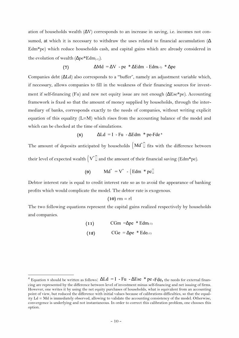
2. Scenario 2: Investment risingThe shock of investment is simulated by a change on g0, in the equation of accumulation.

The constant is fixed over the 2005 period at a level that allows the appearance of an instant­

aneous rise of investment, corresponding to one percent of GDP. Investment is approxim­

ately increase by 4 %, what corresponds to a rate of investment close to 25 % in the vari­

ations of the model. One can observe that the impact is permanent in spite of the instantan­

eous nature of the shock. It leads to an increase in GDP, consumption, investment, wages

and dividends which fluctuate between 0.25 and 0.33 percent compared to the initial path.

The rate of profit and the debt ratio are gradually restored on their starting level, after more

or less strong fluctuations. If long run evolutions converge, short run evolutions are slightly

different. In mode 3.1, during a few periods, consumption is pushed over its initial level both

by the increase in growth and the increase in dividends. The level of undistributed profit is

fixed on investment in the previous period, so that the rate of profit knows the strongest

evolution in terms of amplitude but falls down quickly. In configuration 3.2, profit increases

more slightly. This increase is indirectly fixed on GDP by gross profit. As the gross profit

also defines dividends and as retained profit is a remainder, rate of profit knows a low and

short rise. The oscillation is stronger in the second configuration than in the two others. The

evolutions of GDP and wages are confused. This procyclicity explains the greatest oscilla­

tion of the model. In mode 3.3, the definition of consumption from wages, dividends and

wealth observed at the previous period provoke a counter-cyclical process. After the shock,

investment is compensated as component of total demand by households’ consumption. This

interpretation is confirmed by financial evolution of the variables whose amplitude in last

pattern is more reduce.

Image 2: Increase in investment, equivalent to one percent of GDP

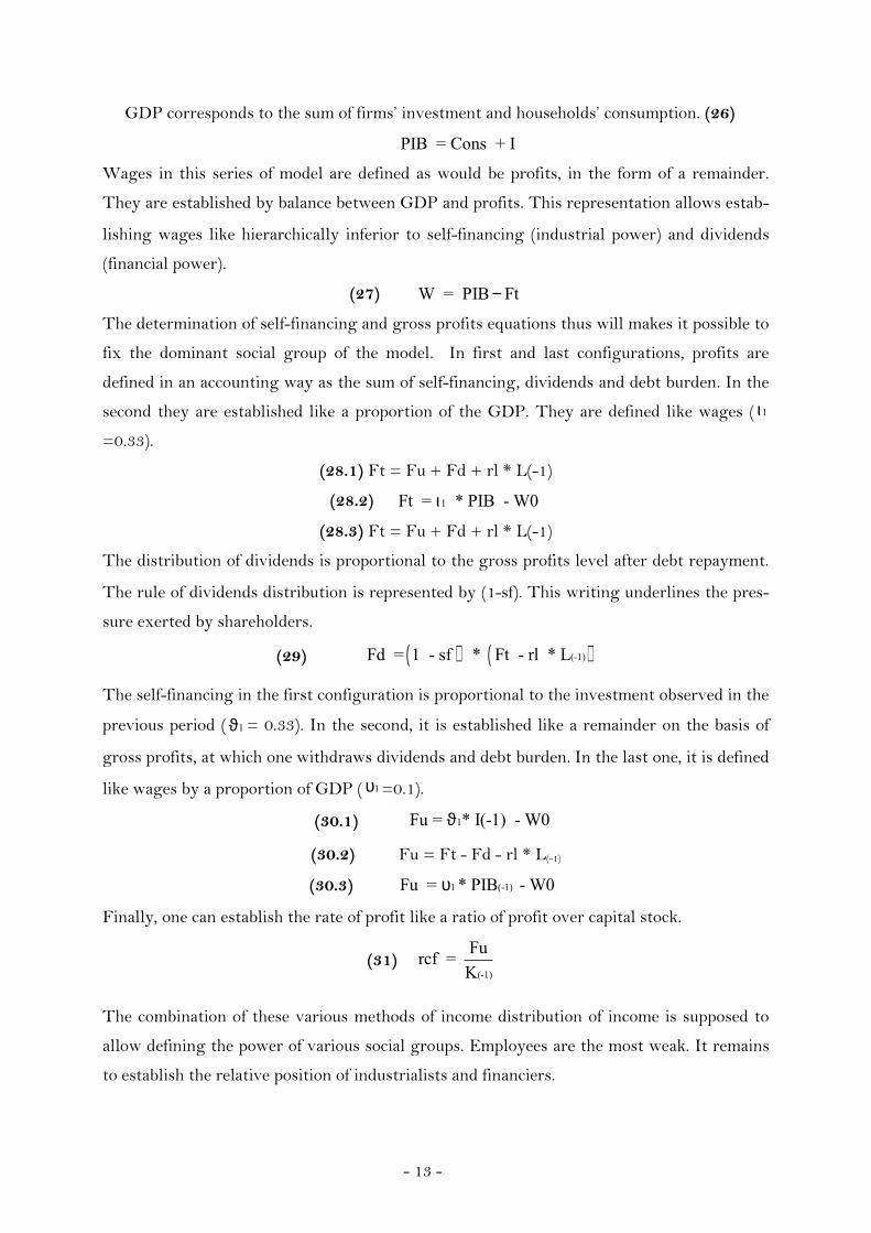
3. Scenario 3: Increase in wages Wage increase is simulated by a final reduction of undistributed profits equivalent to one

percent of GDP of the period 2005. In that way, one underlines the opposition of between

wage and profit. In addition, it is not possible to operate differently considering the defini­

tion of wages as remainder of profits compared to GDP. One of the results in term of interest

conflict also resides in the reduction of financial wealth importance, reducing the power of

finance all the more. In the whole configurations, one can observe contradictory evolutions

between short and long run. Revival effect induced by wages dominates in the short run,

while financial effects of supply recession dominate medium and long run evolutions. The

sign of the evolutions of the three models is identical, but the levels of each configuration can

be rather different. Some symmetry can be observed in the first two regimes, the last one is

- 16 -

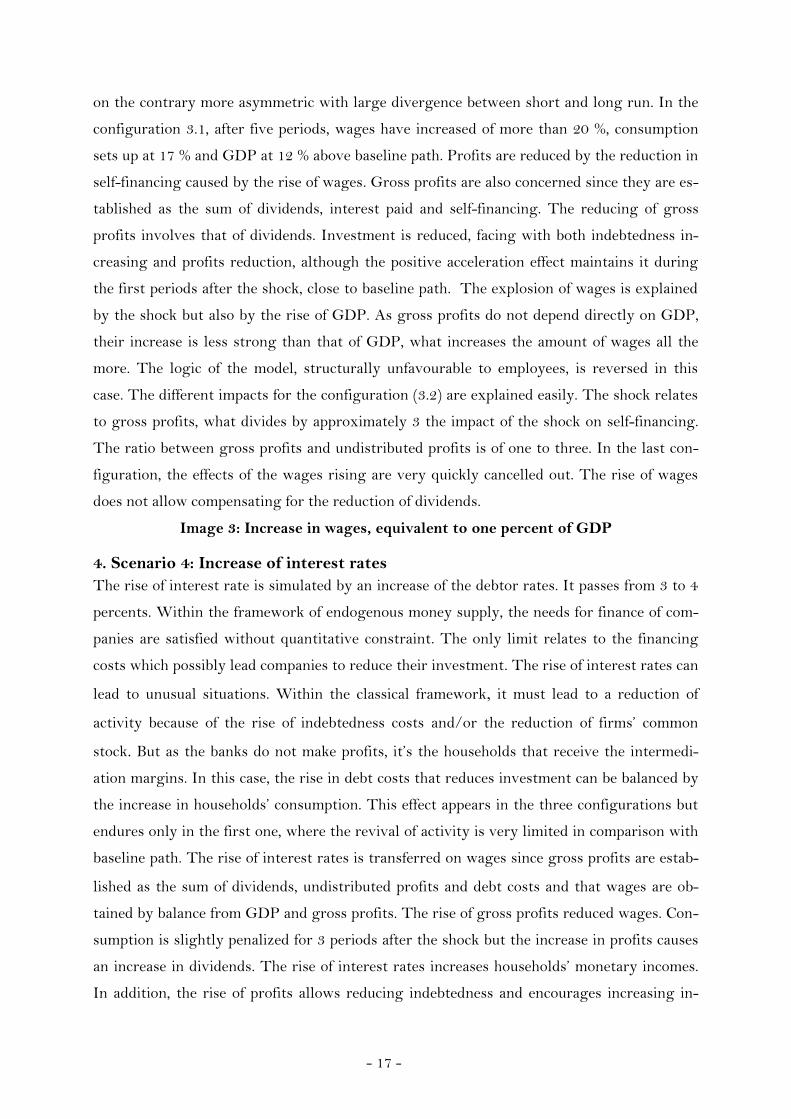
on the contrary more asymmetric with large divergence between short and long run. In the

configuration 3.1, after five periods, wages have increased of more than 20 %, consumption

sets up at 17 % and GDP at 12 % above baseline path. Profits are reduced by the reduction in

self-financing caused by the rise of wages. Gross profits are also concerned since they are es­

tablished as the sum of dividends, interest paid and self-financing. The reducing of gross

profits involves that of dividends. Investment is reduced, facing with both indebtedness in­

creasing and profits reduction, although the positive acceleration effect maintains it during

the first periods after the shock, close to baseline path. The explosion of wages is explained

by the shock but also by the rise of GDP. As gross profits do not depend directly on GDP,

their increase is less strong than that of GDP, what increases the amount of wages all the

more. The logic of the model, structurally unfavourable to employees, is reversed in this

case. The different impacts for the configuration (3.2) are explained easily. The shock relates

to gross profits, what divides by approximately 3 the impact of the shock on self-financing.

The ratio between gross profits and undistributed profits is of one to three. In the last con­

figuration, the effects of the wages rising are very quickly cancelled out. The rise of wages

does not allow compensating for the reduction of dividends.

Image 3: Increase in wages, equivalent to one percent of GDP

4. Scenario 4: Increase of interest ratesThe rise of interest rate is simulated by an increase of the debtor rates. It passes from 3 to 4

percents. Within the framework of endogenous money supply, the needs for finance of com­

panies are satisfied without quantitative constraint. The only limit relates to the financing

costs which possibly lead companies to reduce their investment. The rise of interest rates can

lead to unusual situations. Within the classical framework, it must lead to a reduction of

activity because of the rise of indebtedness costs and/or the reduction of firms’ common

stock. But as the banks do not make profits, it’s the households that receive the intermedi­

ation margins. In this case, the rise in debt costs that reduces investment can be balanced by

the increase in households’ consumption. This effect appears in the three configurations but

endures only in the first one, where the revival of activity is very limited in comparison with

baseline path. The rise of interest rates is transferred on wages since gross profits are estab­

lished as the sum of dividends, undistributed profits and debt costs and that wages are ob­

tained by balance from GDP and gross profits. The rise of gross profits reduced wages. Con­

sumption is slightly penalized for 3 periods after the shock but the increase in profits causes

an increase in dividends. The rise of interest rates increases households’ monetary incomes.

In addition, the rise of profits allows reducing indebtedness and encourages increasing in­

- 17 -

vestment. Total demand increases, what the rise of GDP indicates. In the second configura­

tion, the rise of interest rates generates a reduction of dividends which is not compensated by

the rise of gross profits. Gross profits increase less quickly than GDP, what causes an in­

crease in wages. Retained profits decrease too. Indebtedness increases and investment de­

creases but consumption is led by wages and monetary incomes. In the medium run, the re­

cessionary effects finally appear. In the last configuration, evolutions are less ambiguous be­

cause wages drop and do not take part in the maintenance of consumption. The initial im­

pulse is reduced and negative effects appear much more quickly since consumption function

has a reduced elasticity regarding monetary incomes.

Image 4: Increase of interest rates from 3 to 4 %

5. Scenario 5: Increase of equity issuing

The increase in equity issuing is simulated by a positive variation of the constant τ0 in the

equation (1). It leads to an increase in the equity finance of investment equivalent to one per­

cent of investment of 2005. The raising of the constant is permanent. The expected effects

are an indebtedness reduction and an increase in investment and growth. These are precisely

the results obtained in the three configurations. A negative effect is however present. The di­

lution effect related to the increasing equity issuing but a volume effect compensates for this

fall of prices.

The evolutions are very close for the whole configurations. Investment is the first element

that pushes growth. It is due to indebtedness reduction and to the increase of retained earn­

ings. In the first configuration, gross profits increase less quickly than GDP, what leads to a

clear rise of wages which maintain the demand from employees. The virtuous sequence

between consumption and investment set up. In the second configuration, these are the dis­

tributed profits that increase the most quickly after investment. The rise of the gross profits

also induces an increase in undistributed profits. One observes that a driving force slightly

less important for the third configuration. Investment deviates slightly from the other vari­

ables contrary to the first two configurations. Consumption is lower than in the baseline dur­

ing the first periods following the shock, whereas wages and distributed dividends increase

but more slightly than in previous situations. In same time, monetary incomes decrease, and

shareholders sustain capital losses.

Image 5: Increase of equity issuing, equivalent to one percent of GDP

- 18 -

6. Scenario 6: Increase in households’ equities

The rise of household shareholding is simulated through the increase in ψ0, the constant in

the equation (3) which determines the household portfolio behaviour. This variation aims at

increasing by one percent the share of equities in household financial capital. It passes from

approximately 43 % to more than 44 %. Contrary to preceding scenarios, this shock gener­

ates effects that are specifics to each configuration, with a surprising effect for the first,

namely an evolution which becomes negative in the long run. In spite of some contradictory

oscillations in the medium run, the two following ones converge in the long run towards the

expected results, but with weak effects on growth since after 40 periods, GDP is only little

one percent above the reference scenario. For more financial aspects, one finds the opposition

between evolution of equity prices and evolution of total portfolio of equities held, which is

explained by diversification phenomena generated by the stability of the actors’ portfolio be­

haviour.

The configuration (3.1) diverges from expectations. Instantaneously after the shock, invest­

ment reduces while one observes an increase of indebtedness contradictory with intuition of

an increase of firms shareholders’ equity. During the very first periods, firms increase their

financial investments, because of the rising equity prices initiated by the increase of house­

holds demand. An opposition appears between real economy and financial economy. This

first movement is symmetrical to increasing wages, consumption and GDP. It is induced by

the reduction of self-financing caused by investment reduction. Undistributed profit is a

function of last-period investment. The reduction of self-financing impacts negatively gross

profits, what increases wages. Investment is restored by demand acceleration effects as well

as profit recovery and debt reduction. But growth does not manage to stabilize and fall

again. Consumption alone is not able to lead investment. The fixing of self-financing on

former investment harms capacity of finance which results in an inescapable increase of in­

debtedness. In configuration 3.2, one finds the increase in short-run indebtedness caused by

the financial investments of firms. The definition of self-financing less unfavourable to firms

in the last configurations allows to reduce the debt and finally to relaunch investment.

Image 6: Increase in households’ equities, equivalent to one percent of their financial

wealth

7. Scenario 7: Increase in dividends

The dividends increase is simulated by the reduction of (sf) in the equation (29) establishing

the distribution of profits. Initially, dividends represent 18 % of GDP, or 64 % of gross

profits. The shock consists in increasing them by one percent of GDP. Dividends reach to 19

- 19 -

% of GDP. Expected results are related to the nature of pattern. The rise of dividends is fin­

anced either by a reduction of self-financing, or by a cut in wages. The question posed here is

to know if the fall of investment in the first case or consumption in the second will be com­

pensated by an increase in firms and households financial funds. In last configuration, there

is no ambiguity. In the short run, like in the long run, the increase in dividends allows to

compensate for the cut in wages. This process is facilitated by the modification of consump­

tion equation where propensity to consume wages has been reduced. The fall of earned in­

comes less strongly impacts consumption. Moreover, the way of establishing profits does not

penalize firms account since the shock is deferred on wages. Indebtedness is reduced, which

supports investment. In addition, the impact on firms of dividend increase is limited insofar

as firms take advantage too of this rise as shareholders. In the second configuration, these

are undistributed profits that are used to finance the rise of dividends. Consumption is led by

financial incomes, but firms’ accounts are penalized. The increase in investment cannot be

maintained. GDP evolution which is confused with wages one becomes clearly negative a

shortly before the fortieth period. In configuration 3.1 total evolution is symmetrical. Adjust­

ment relates to wages, while firms defer the whole financial constraints on employees. Con­

sumption follows the wages which know a negative evolution. On the contrary, firms invest

more because of the reduction of their indebtedness level partly thanks to the rise of di­

vidends which is set on gross profits. The reduction of wages inflated gross profits, which

explains the surge of dividends. The maintenance of investment makes it possible to contain

the fall of activity. The rise of dividends finally manages to compensate for the cut in wages.

The total demand is relaunched 5 periods after the shock and recovers a level closed to the

baseline at the 25th period.

Image 7: Increase in dividends, equivalent to one percent of GDP

8. Scenario 8: Share buybacks by firms

In this last scenario, one increases by one percent of firms’ shareholding by the variation of

the constant η0. The share buyback policies are becoming numerous. Through this policy,

firms try to increase shareholder value, to prevent from unfriendly takeovers and to increase

their absorption capacity. All these elements of industrial economy cannot be recalled within

the macroeconomic framework that one chose to mobilize. Attention is focused on the mac­

roeconomic consequences of such practices. Effects are unspecified a priori, because the cash

used in share buybacks is of course not used for productive investment, but income flows

could be used for sellers’ consumption. At macroeconomic level, this effect of leak from cir­

cuit disappears. By contrast, the increase in equity prices constitutes a potential escape, a

- 20 -

kind of inflation, if it does not correspond to an equivalent increase of produced value when

equities will be resold6.

This ambivalence shows through in the whole configurations where the first movement is a

decline of activity related to the increase of indebtedness. The question of the debt ratio used,

debt over fixed capital stock, can be asked insofar as one notices at the same time an increase

in financial wealth. A financial illusion process could intervene in reality, especially in a con­

text of regular increase in equity prices which would not penalize investment and could gen­

erate a cumulative dynamics which does not appear in the model. In the configuration (3.1),

the positive effects of share buyback appears after forty periods, in the second, it is necessary

to wait 75 periods. Coherence of the third configuration seems stronger. Positive effects ap­

pear after 15 periods. The configuration (3.2) is the clearest to interpret. Financial invest­

ment generates indebtedness which penalizes physical investment. Once first shock wave is

absorbed, indebtedness decreases and rate of profit is stabilized whereas wages, consumption

and growth continue to decrease. Thereafter, the reduction of indebtedness allows a resur­

gence of investment. This one leads growth, wages, dividends and consumption. Economy

breaks the deadlock. The procyclic nature of pattern explains the depth of crisis. Gross

profits fixed on GDP collapse with GDP. Undistributed profits followed and suffer the rise

of indebtedness in addition. In the configuration (3.1), undistributed profits are fixed on past

investment, what allows containing cumulative fall. Gross profit corresponds to the sum of

distributed, undistributed profits, and debt service. The fall of undistributed profits is con­

tained, while debt service increases. On the other hand, consumption and GDP know a more

unfavourable evolution than in the configuration (3.2) in the short run, but it is less endur­

ing. The good shape of gross profits gives rise to important dividends which allow consump­

tion resurgence. The configuration (3.3) experiences a short term evolution less unfavour­

able than the first one, but its long-term evolution is less sustained. After the shock, it is the

only one which maintains consumption. Gross profits are slightly reduced. This involves

wage increase, reinforced by the increase in monetary incomes. Investment decline is par­

tially compensated by the maintenance of consumption. The shock is quickly absorbed be­

cause of the weak impact on investment and consumption. Indebtedness is less strongly re­

duced than in the configuration (3.1) what explains the less strong slope of investment. Fi­

6 If an important gap is observed between fundamental and nominal equity values at the time of equity resale, a

process of depreciation process can occur. The rise in equity prices would have been drove by demand the

request during the launching of pension funds. Reached to maturity, capitalized pension system could involve a

fall of equity prices or inflation because of selling, what comes to the same thing as far as purchasing power is

concerned.

- 21 -

nally, the differences between configurations seem to be sum up through the significance of

equity prices evolution. Where financial wealth are the most developed, indebtedness is most

reduced, which supports growth.

Image 8: Increase of one percent of share buybacks by firms

Conclusion

The method developed by the neo-Cambridgian approach seems able to recount specificities

of finance-led capitalism. Structural models make it possible to specify the whole flows and

stocks links, influence of wealth effects and leverage. The regulation theory allows specifying

the transformations that took place in contemporary capitalism through the inversion of in­

stitutional hierarchy, the rise of financial power and the backward flow of the worker power.

The most salient results that one can retain of these various experiments relate to the oppos­

ition between wage increase which plays negatively as expected in a financialized regime,

and rise in dividends which on the contrary plays positively in two cases out of three. These

contradictory evolutions allow providing theoretical elements to explain divergences

between France and the United States within the framework of a closed and financialized

economy. France faced with an absence of consistent institutions that relates at the same

time to the economy structures, its place in the world economy and also its regulation mode

which remains marked by the heritage of fordian period.

From an economic point of view, France got into financialization. However, from a political

point of view thus concerning the mode of regulation, resistances appear about the complete

adoption of a financialized regime. The increase in inequalities which are bound there, ex­

cluding nature of finance-led regime, generate a political resistance. Also, France entered a

financialized accumulation pattern constrained by extra-economic elements which do not

prevent reduced and profitable capital accumulation but which are durably far away from the

full employment. In order to attain a sustained high growth within a framework of increas­

ing financialization, some institutional complementarities must emerge. In their absence, fin­

ancial burden penalizes economic growth. In the model presented in this work, firms profit

from financial dynamics as shareholder. Thus, when firms are not penalized by the form of

income distribution, growth can be more constant.

These results however are conditioned by a strong household’s involvement in the financial

markets. However, this one is very uneven, even in the United States. In France, this in­

volvement is more reduced in level, but it is as well concentrated. Financial wealth effects ac­

tually appeared in the United States, but real estate wealth effects have been more powerful,

relegated by rising of households’ debt. So as to identify an accumulation pattern, it is neces­

- 22 -

sary to establish the dynamic coherence of the American economic system. With this inten­

tion, one cannot elude international regime question which is not treated in present models

which are closed. Consequently, even if these models are able to account for the first Regula­

tionnists intuitions about the existence of a patrimonial regime, they cannot describe reality

of the American macroeconomic closing within this framework still too narrow. To approach

the real functioning of the American economy, the model should be open; households should

be able to run into debt and to hold real estate assets.

In a theoretical point of view, the model meets some limits. Concerning the treatment of

equity prices, on has tried to obtain a model where these ones are determined endogenously,

but this lead to some paradoxical portfolio behaviours. An exogenous determination of

equity prices should be experiment. The theoretical framework of endogenous money is not

well-fitted to describe financialized regime where companies observe financial constraints.

Finally, to improve the model, it could be interesting to introduce on one hand two types of

households (poor and rich ones) where the first ones depends on wage to consume and the

second ones only on dividends and capital gains, and on the other hand two sectors, small

and big companies, differentiated by their access to equity finance and by they participation

in general to stock market dynamics.

Bibliography:

AGLIETTA, M. (1998), “Le Capitalisme de demain”, Note de la fondation Saint-Simon, n° 101,

novembre.

AGLIETTA, M. (2000), “Shareholder value and corporate governance: some tricky questions”,

Economy and Society, vol. 29, n°1, February, pp. 146-159.

AGLIETTA, M. & BRETON, R. (2001), “Financial Systems, Corporate Control, and Capital Accu­

mulation”, Economy and Society, vol. 30, n°4, November, pp. 433-466.

AGLIETTA, M. & REBÉRIOUX A. (2004), L’instabilité du capitalisme financier, Paris: Albin Michel.

AMABLE, B. (2005), Les cinq Capitalismes. Diversité des systèmes économiques et sociaux dans la

mondialisation, coll. Economie Humaine, Paris: Seuil.

ARTUS, P. & VIRARD, M.-P. (2005), Le capitalisme est en train de s’autodétruire, Paris: La

Découverte.

ASKÉNAZY, P. (2003), “Partage de la valeur ajoutée et rentabilité du capital en France et aux

États-Unis : une réévaluation”, Economie et Statistique, n°363-364, pp.167-186.

Available at http://www.insee.fr/fr/ffc/docs_ffc/es363-364-365i.pdf

ASKÉNAZY, P. (2004), Les Désordres du travail. Enquête sur le nouveau productivisme, coll. La

république des idées, Paris: Seuil.

- 23 -

BEN GAMRA, S. & CLÉVENOT, M. (2006), “Libéralisation financière et crises bancaires dans les

pays tiers. La prégnance du rôle des institutions”, CEPN Working papers, n° WP2006-08.

Available at http:// www.univ-paris13.fr/CEPN/wp2006_08.pdf

BOYER, R. (1978), “L'évolution des salaires en longue période”, Economie et Statistique, n°103,

pp. 27-57.

BOYER, R. (2000), “Is a finance-led growth regime a viable alternative to Fordism ? A prelim­

inary analyse”, Economy and Society, vol. 29, n°1, February, pp. 111-145.

CLÉVENOT, M. (2003), “Les méthodes développées par la Stock Flow Consistent Approach à la

lumière de la Théorie de la Régulation”, Actes du Forum de la régulation, 9-10 octobre. Avail­

able at

http:// web.upmf-grenoble.fr/regulation/Forum/Forum_2003/Forumpdf/RR_CLEV ­

ENOT.pdf

CLÉVENOT, M. (2006), Financiarisation, régime d'accumulation et mode de régulation. Peut-on

appliquer le ”modèle” américain à l'économie française ?, Ph.D. Thesis, University Paris Nord -

Paris XIII - (08/12/2006).

Available at

https://hal.ccsd.cnrs.fr/view_by_stamp.php?label=CNRS&langue=fr&action_todo=view&id

=tel-00120886&version=1

CLÉVENOT, M., GUY, Y. & MAZIER, J. (2007), “Investment and rate of profit in a financial con­

text. The French case”, unpublished paper.

FOLEY, D. K. (1975), “On Two Specifications of Asset Equilibrium in Macroeconomic Mod­

els”, Journal of Political Economy, vol. 83, n°2, April, pp. 303-324.

GODLEY, W. (1999), “Money and Credit in a Keynesian Model of Income Determination”,

Cambridge Journal of Economics, vol. 23, n°4, July, pp. 393-411.

LAVOIE, M. & GODLEY, W. (2001), “Kaleckian models of growth in a coherent stock-flow mon­

etary framework: a Kaldorian view”, Journal of Post Keynesian Economics, vol. 24, n°2, pp. 277-

312.

LEHNERT, A. (2004), “Housing, Consumption, and Credit Constraints”, Finance and Economics

Discussion Series, Board of Governors of the Federal Reserve System, n°2004-63.

Available at http://www.federalreserve.gov/pubs/feds/2004/200463/200463pap.pdf

TAYLOR, L. (2004a), “Exchange Rate Indeterminacy in Portfolio Balance, Mundell-Fleming

and Uncovered Interest Rate Parity Models”, Cambridge Journal of Economics, vol. 28, n°2,

pp. 205-227.

TAYLOR, L. (2004b), Reconstructing macroeconomics: structuralist proposals and critiques on the

mainstream, Cambridge MA: Harvard University Press.

- 24 -

-2

0

2

4

6

8

10

2000 2010 2020 2030 2040 2050 2060 2070 2080 2090 2100

Picture 3

-20

-10

0

10

20

2000 2010 2020 2030 2040 2050 2060 2070 2080 2090 2100

Picture 4

-2

0

2

4

6

8

10

2000 2010 2020 2030 2040 2050 2060 2070 2080 2090 2100

Picture 5

-20

-10

0

10

20

2000 2010 2020 2030 2040 2050 2060 2070 2080 2090 2100

Picture 6

-2

0

2

4

6

8

10

2000 2010 2020 2030 2040 2050 2060 2070 2080

GDPConsumptionInvestmentRate of profit DebtWagesDividends

Picture 1

-20

-10

0

10

20

2000 2010 2020 2030 2040 2050

Equity pricesNumber of equityFinancial wealthHousehold's equitiesEquities held by firms

Picture 2

Configuration 1 Configuration 2 Configuration 3

Scenario 1 : Increase in consumption, equivalent to one percent of GDP

- 25 -

-1

0

1

2

3

4

5

2000 2002 2004 2006 2008 2010 2012 2014 2016 2018 2020

Picture 11

-1

0

1

2

3

2000 2005 2010 2015 2020 2025 2030

Picture 12

-1

0

1

2

3

4

5

2000 2005 2010 2015 2020 2025 2030 2035 2040 2045 2050Picture 8

-1

0

1

2

3

2000 2010 2020 2030 2040 2050 2060

Picture 9

-1

0

1

2

3

4

5

2000 2005 2010 2015 2020 2025 2030 2035 2040

GDP

Consumption

Investment

Rate of profit

Debt

Wages

Dividends

Picture 10

-1

0

1

2

3

2000 2005 2010 2015 2020 2025 2030 2035 2040

Equity prices

Number of equity

Financial wealth

Household's equities

Equities held by the firms

Picture 7

Configuration 1 Configuration 2 Configuration 3

Scenario 2 : Increase in investment, equivalent to one percent of GDP

- 26 -

-100

0

100

200

300

2000 2010 2020 2030 2040 2050 2060 2070 2080 2090 2100

Picture 16

-30

-20

-10

0

10

20

30

2000 2010 2020 2030 2040 2050 2060 2070 2080 2090 2100

Picture 15

-30

-20

-10

0

10

20

30

2000 2010 2020 2030 2040 2050 2060 2070 2080 2090 2100

Picture 17

-100

0

100

200

300

2000 2010 2020 2030 2040 2050 2060 2070 2080 2090 2100

Picture 18

-30

-20

-10

0

10

20

30

2000 2010 2020 2030 2040 2050 2060 2070 2080 2090 2100

GDPConsumptionInvestmentRate of profitDebtWagesDividends

Picture 13

-100

0

100

200

300

2000 2010 2020 2030 2040 2050 2060 2070 2080 2090 2100

Equity pricesNumber of equityFinancial wealthHousehold's equities Equities held by firms

Picture 14

Configuration 1 Configuration 2 Configuration 3

Scenario 3 : Increase in wages, equivalent to one percent of GDP

- 27 -

-30

-20

-10

0

10

20

30

2000 2005 2010 2015 2020 2025 2030 2035 2040 2045 2050

Equity pricesNumber of equityFinancial wealthHousehold's equitiesEquities held by firms

Picture 20

-6

-5

-4

-3

-2

-1

0

1

2

3

2000 2005 2010 2015 2020 2025 2030 2035 2040 2045 2050

GDPConsumptionInvestmentRate of profitDebtWagesDividends

Picture 19

-6

-5

-4

-3

-2

-1

0

1

2

3

2000 2005 2010 2015 2020 2025 2030 2035 2040 2045 2050

Picture 23

-30

-20

-10

0

10

20

30

2000 2005 2010 2015 2020 2025 2030 2035 2040 2045 2050

Picture 24

-6

-5

-4

-3

-2

-1

0

1

2

3

2000 2005 2010 2015 2020 2025 2030 2035 2040 2045 2050

Picture 21

-30

-20

-10

0

10

20

30

2000 2005 2010 2015 2020 2025 2030 2035 2040 2045 2050

Picture 22

Configuration 1 Configuration 2 Configuration 3

Scenario 4 : Increase of interest rates from 3 to 4 %

- 28 -

-1

0

1

2

3

4

2000 2005 2010 2015 2020 2025 2030 2035 2040

Picture 29

-20

-10

0

10

20

2000 2005 2010 2015 2020 2025 2030 2035 2040

Picture 30

-1

0

1

2

3

4

2000 2005 2010 2015 2020 2025 2030 2035 2040

PIBConsommationInvestissementTaux de profitEndenttementSalaires Profits distribués

Picture 25

-20

-10

0

10

20

2000 2005 2010 2015 2020 2025 2030 2035 2040

Equity pricesNumber of equityFinancial wealthHousehold's equitiesEquity held by firms

Picture 26

-1

0

1

2

3

4

2000 2005 2010 2015 2020 2025 2030 2035 2040

Picture 27

-20

-10

0

10

20

2000 2005 2010 2015 2020 2025 2030 2035 2040

Picture 28

Configuration 1 Configuration 2 Configuration 3

Scenario 5 : Increase of equity issuing, equivalent to one percent of GDP

- 29 -

-2

-1

0

1

2

2000 2005 2010 2015 2020 2025 2030 2035 2040

Picture 41

-40

-20

0

20

40

60

2000 2005 2010 2015 2020 2025 2030 2035 2040

Picture 42

-2

-1

0

1

2

2000 2005 2010 2015 2020 2025 2030 2035 2040

Picture 39

-40

-20

0

20

40

60

2000 2005 2010 2015 2020 2025 2030 2035 2040

Picture 40

-2

-1

0

1

2

2000 2010 2020 2030 2040 2050 2060 2070 2080 2090 2100

GDPConsumptionInvestmentRate of profitDebtWagesDividends

Picture 37

-40

-20

0

20

40

60

2000 2010 2020 2030 2040 2050 2060 2070 2080 2090 2100

Equity pricesNumber of equityFinancial wealthHousehold's equitiesEquities held by firms

Picture 38

Configuration 1Configuration 2 Configuration 3

Scenario 6 : Increase in households’ equities, equivalent to one percent of their financial wealth

- 30 -

-5

0

5

10

15

20

25

2000 2005 2010 2015 2020 2025 2030 2035 2040

Picture 41

-40

-20

0

20

40

60

80

2000 2005 2010 2015 2020 2025 2030 2035 2040

Picture 42

-5

0

5

10

15

20

25

2000 2005 2010 2015 2020 2025 2030 2035 2040 2045 2050

GDPConsumptionInvestmentRate of profitDebtWagesDividends

Picture 37

-40

-20

0

20

40

60

80

2000 2005 2010 2015 2020 2025 2030 2035 2040 2045 2050

Equity pricesNumber of equityFinancial wealthHousehold's equitiesEquities held by firms

Picture 38

-5

0

5

10

15

20

25

2000 2010 2020 2030 2040 2050 2060 2070 2080 2090 2100

Picture 39

-40

-20

0

20

40

60

80

2000 2010 2020 2030 2040 2050 2060 2070 2080 2090 2100

Picture 40

Configuration 1 Configuration 2 Configuration 3

Scenario 7 : Increase in dividends, equivalent to one percent of GDP

- 31 -

-40

0

40

80

2000 2010 2020 2030 2040 2050 2060 2070 2080 2090 2100

Picture 48

-5

0

5

10

15

2000 2010 2020 2030 2040 2050 2060 2070 2080 2090 2100

Picture 47

-5

0

5

10

15

2000 2010 2020 2030 2040 2050 2060 2070 2080 2090 2100

GDPConsumptionInvestmentRate of profitDebtWagesDividends

Picture 43

-40

0

40

80

2000 2010 2020 2030 2040 2050 2060 2070 2080 2090 2100

Equity pricesNumber of equityFinancial wealthHousehold's equitiesEquities held by firms

Picture 44

-5

0

5

10

15

2000 2010 2020 2030 2040 2050 2060 2070 2080 2090 2100

Picture 45

-40

0

40

80

2000 2010 2020 2030 2040 2050 2060 2070 2080 2090 2100

Picture 46

Configuration 1 Configuration 2 Configuration 3

Scenario 8 : Increase of one percent of share buybacks by firms

- 32 -

Table 3. Summarization of the three configurations

(1) ( )-1

1 2 0ΔEs * pe L = * + * rl +

I Fu τ τ τ

(2) ( )( ) ( ) ( )1 -1 2 -1 0Ede * pe = * ree + * rcf +

Ede * pe + Kη η η∆

(3)*

1 2 3 0* *

pe*Edm Yhr = * rm + * rem(-1) + * + V V

ψ ψ ψ ψ

(4) Ed = Edm + Ede (5) Ese = Es - Ede (6) Edm = Ese (7) (-1)Md = V - pe * Edm - Edm * pe∆ ∆ ∆ ∆ (8) Ld = I - Fu - Edm * pe-Fde∆ ∆ (9) ( )* *Md = V - Edm * pe(10) rm = rl(11) (-1)CGm = pe * Edm∆(12) (-1)CGe = pe * Ede∆

(13) EdmFdm = Fd *Es

(14) EdeFde = Fd *Es

(15) ( )

( )(-1) (-1)

Fde + CGeree =

pe * Ede

(16) ( )

( )(-1)

Fdm + CGmrem =

pe(-1) * Edm(17) V = Yhr - Cons + CGm∆(18) * *

(-1)V = V + Yhr + CGm - Cons(20) (-1)Yhr = W + Fdm + rm * M

(21) (-1)

Yhr gy = Yhr∆

(22) *(-1) (-1)Yhr = (1 + gy ) * Yhr

(23) ( ) (-1)1 -1 2 3 0

(-1) (-1)

LΔPIBg = * rcf - * + * + K PIB

φ φ φ φ

(24) (-1)I = g * K (25) (-1)K = K * (1 - + g)δ(26) PIB = Cons + I

(31) (-1)

Furcf = K

Configuration 3.1 (19.1) *

0 1 2 (-1)Cons = + * Yhr + * Vα α α(27.1) W = PIB Ft−(28.1) Ft = Fu + Fd + rl * L(-1)(29.1) ( ) ( )(-1)Fd = 1 - sf * Ft - rl * L(30.1) 1 0 Fu = * I(-1) - Wϑ Configuration 3.2 (19.2) *

0 1 2 (-1)Cons = + * Yhr + * Vα α α (27.2) W = PIB Ft− (28.2) 1 0Ft = * PIB - Wι (29.2) ( ) ( )(-1)Fd = 1 - sf * Ft - rl * L (30.2) (-1)Fu = Ft - Fd - rl * LConfiguration 3.3(19.3) 0 11 (-1) 12 (-1) 13 (-1) 2 (-1)Cons = + *W + * Fd + *rl*L + * Vα α α α α (27.3) W = PIB Ft−(28.3) (-1)Ft = Fu + Fd + rl * L(29.3) ( ) ( )(-1)Fd = 1 - sf * Ft - rl * L(30.3) Fu = υ1*PIB(-1) –W0

- 33 -