Network meta-analysis & models for inconsistency
66
Network meta-analysis & models for inconsistency Centre for Health Economics, University of York 15 th January 2015 Ian White MRC Biostatistics Unit, Cambridge, UK
-
Upload
cheweb1 -
Category
Health & Medicine
-
view
261 -
download
0
Transcript of Network meta-analysis & models for inconsistency

Network meta-analysis & models for inconsistency
Centre for Health Economics, University of York
15th January 2015
Ian White
MRC Biostatistics Unit, Cambridge, UK
Motivation
• Systematic review is essential to draw evidence-based conclusions
• Usually use meta-analysis to give a statistical summary of the evidence
• Often this involves simple comparisons - e.g. "Is streptokinase effective after myocardial infarction?"
• But often multiple interventions are available
– clinicians and policy-makers want to know what the best intervention is
– e.g. NICE multiple technology assessment
• Network meta-analysis aims to provide a statistical summary of the evidence about all interventions available for a particular patient group
Plan
• Meta-analysis
• Indirect comparisons
• Network meta-analysis
– models allowing for heterogeneity
– models allowing for inconsistency
– model estimation
– examples
– controversies
3
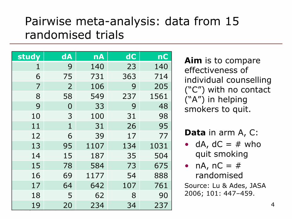
Pairwise meta-analysis: data from 15 randomised trials
4
study dA nA dC nC
1 9 140 23 140
6 75 731 363 714
7 2 106 9 205
8 58 549 237 1561
9 0 33 9 48
10 3 100 31 98
11 1 31 26 95
12 6 39 17 77
13 95 1107 134 1031
14 15 187 35 504
15 78 584 73 675
16 69 1177 54 888
17 64 642 107 761
18 5 62 8 90
19 20 234 34 237
Aim is to compare effectiveness of individual counselling (“C”) with no contact (“A”) in helping smokers to quit.
Data in arm A, C:
• dA, dC = # who quit smoking
• nA, nC = # randomised
Source: Lu & Ades, JASA 2006; 101: 447–459.
Data display: Forest plot
5
ID
9
10
14
8
16
15
1
7
11
13
17
12
18
19
6
Study
Odds ratio (95% CI)
16.11 (0.90, 287.30)
14.96 (4.39, 50.94)
0.86 (0.46, 1.61)
1.52 (1.12, 2.06)
1.04 (0.72, 1.50)
0.79 (0.56, 1.11)
2.86 (1.27, 6.43)
2.39 (0.51, 11.26)
11.30 (1.47, 87.18)
1.59 (1.21, 2.10)
1.48 (1.06, 2.05)
1.56 (0.56, 4.33)
1.11 (0.35, 3.57)
1.79 (1.00, 3.22)
9.05 (6.83, 11.97)
Odds ratio (95% CI)
16.11 (0.90, 287.30)
14.96 (4.39, 50.94)
0.86 (0.46, 1.61)
1.52 (1.12, 2.06)
1.04 (0.72, 1.50)
0.79 (0.56, 1.11)
2.86 (1.27, 6.43)
2.39 (0.51, 11.26)
11.30 (1.47, 87.18)
1.59 (1.21, 2.10)
1.48 (1.06, 2.05)
1.56 (0.56, 4.33)
1.11 (0.35, 3.57)
1.79 (1.00, 3.22)
9.05 (6.83, 11.97)
favours A favours C 1.2 .5 1 2 5 10 20
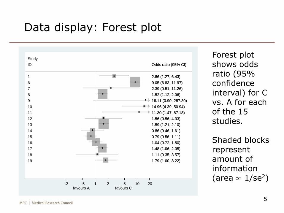
Forest plot shows odds ratio (95% confidence interval) for C vs. A for each of the 15 studies.
Shaded blocks represent amount of information (area 1/se2)
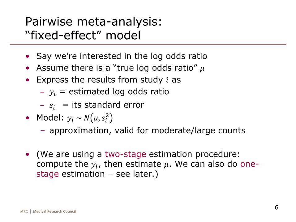
Pairwise meta-analysis: “fixed-effect” model
• Say we’re interested in the log odds ratio
• Assume there is a “true log odds ratio” 𝜇
• Express the results from study 𝑖 as
– 𝑦𝑖 = estimated log odds ratio
– 𝑠𝑖 = its standard error
• Model: 𝑦𝑖 ~ 𝑁 𝜇, 𝑠𝑖2
– approximation, valid for moderate/large counts
• (We are using a two-stage estimation procedure: compute the 𝑦𝑖, then estimate 𝜇. We can also do one-stage estimation – see later.)
6
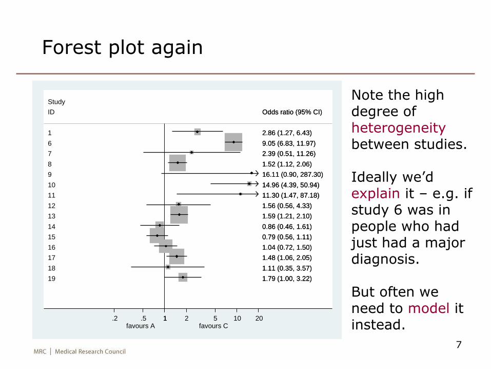
Forest plot again
7
Note the high degree of heterogeneitybetween studies.
Ideally we’d explain it – e.g. if study 6 was in people who had just had a major diagnosis.
But often we need to model it instead.
ID
9
10
14
8
16
15
1
7
11
13
17
12
18
19
6
Study
Odds ratio (95% CI)
16.11 (0.90, 287.30)
14.96 (4.39, 50.94)
0.86 (0.46, 1.61)
1.52 (1.12, 2.06)
1.04 (0.72, 1.50)
0.79 (0.56, 1.11)
2.86 (1.27, 6.43)
2.39 (0.51, 11.26)
11.30 (1.47, 87.18)
1.59 (1.21, 2.10)
1.48 (1.06, 2.05)
1.56 (0.56, 4.33)
1.11 (0.35, 3.57)
1.79 (1.00, 3.22)
9.05 (6.83, 11.97)
Odds ratio (95% CI)
16.11 (0.90, 287.30)
14.96 (4.39, 50.94)
0.86 (0.46, 1.61)
1.52 (1.12, 2.06)
1.04 (0.72, 1.50)
0.79 (0.56, 1.11)
2.86 (1.27, 6.43)
2.39 (0.51, 11.26)
11.30 (1.47, 87.18)
1.59 (1.21, 2.10)
1.48 (1.06, 2.05)
1.56 (0.56, 4.33)
1.11 (0.35, 3.57)
1.79 (1.00, 3.22)
9.05 (6.83, 11.97)
favours A favours C 1.2 .5 1 2 5 10 20
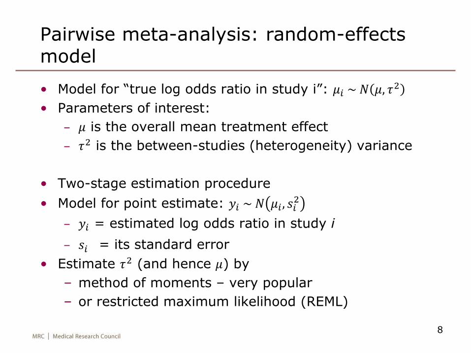
Pairwise meta-analysis: random-effects model
• Model for “true log odds ratio in study i”: 𝜇𝑖 ~ 𝑁 𝜇, 𝜏2
• Parameters of interest:
– 𝜇 is the overall mean treatment effect
– 𝜏2 is the between-studies (heterogeneity) variance
• Two-stage estimation procedure
• Model for point estimate: 𝑦𝑖 ~ 𝑁 𝜇𝑖 , 𝑠𝑖2
– 𝑦𝑖 = estimated log odds ratio in study i
– 𝑠𝑖 = its standard error
• Estimate 𝜏2 (and hence 𝜇) by
– method of moments – very popular
– or restricted maximum likelihood (REML)
8
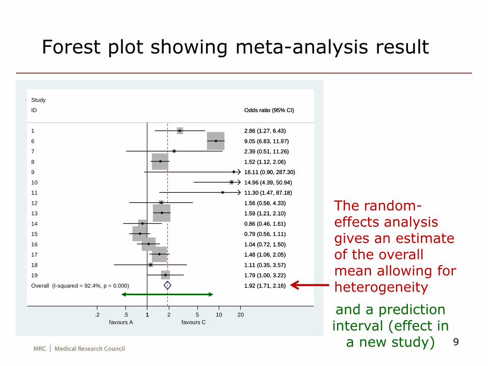
Overall (I-squared = 92.4%, p = 0.000)
ID
9
10
14
8
16
15
1
7
11
13
17
12
18
19
6
Study
1.92 (1.71, 2.16)
Odds ratio (95% CI)
16.11 (0.90, 287.30)
14.96 (4.39, 50.94)
0.86 (0.46, 1.61)
1.52 (1.12, 2.06)
1.04 (0.72, 1.50)
0.79 (0.56, 1.11)
2.86 (1.27, 6.43)
2.39 (0.51, 11.26)
11.30 (1.47, 87.18)
1.59 (1.21, 2.10)
1.48 (1.06, 2.05)
1.56 (0.56, 4.33)
1.11 (0.35, 3.57)
1.79 (1.00, 3.22)
9.05 (6.83, 11.97)
favours A favours C
1.2 .5 1 2 5 10 20
Forest plot showing meta-analysis result
9
The random-effects analysis gives an estimate of the overall mean allowing for heterogeneity
and a prediction interval (effect in
a new study)
Other issues in (pairwise) meta-analysis
• Study quality
• Study-level covariates “meta-regression”
• Publication bias
– small trials more likely to be published if they show statistically significant effects?
10
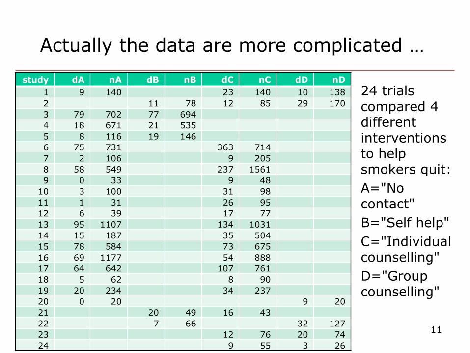
Actually the data are more complicated …
11
study dA nA dB nB dC nC dD nD
1 9 140 23 140 10 138
2 11 78 12 85 29 170
3 79 702 77 694
4 18 671 21 535
5 8 116 19 146
6 75 731 363 714
7 2 106 9 205
8 58 549 237 1561
9 0 33 9 48
10 3 100 31 98
11 1 31 26 95
12 6 39 17 77
13 95 1107 134 1031
14 15 187 35 504
15 78 584 73 675
16 69 1177 54 888
17 64 642 107 761
18 5 62 8 90
19 20 234 34 237
20 0 20 9 20
21 20 49 16 43
22 7 66 32 127
23 12 76 20 74
24 9 55 3 26
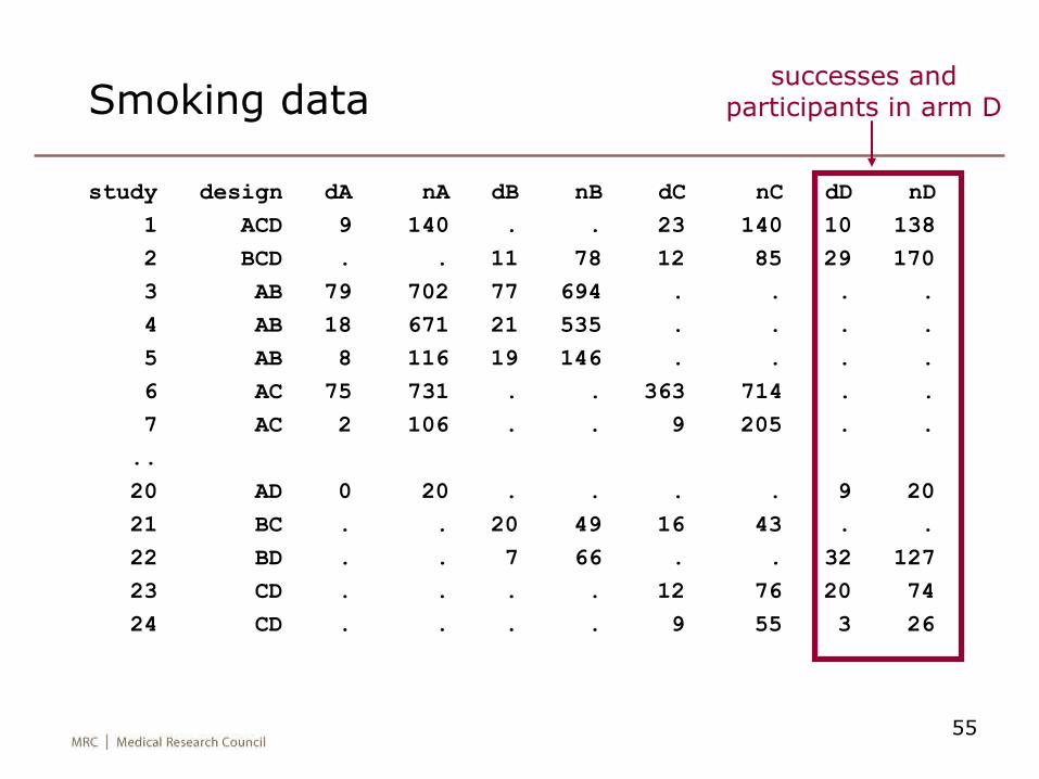
24 trials compared 4 different interventions to help smokers quit:
A="No contact"
B="Self help"
C="Individual counselling"
D="Group counselling"
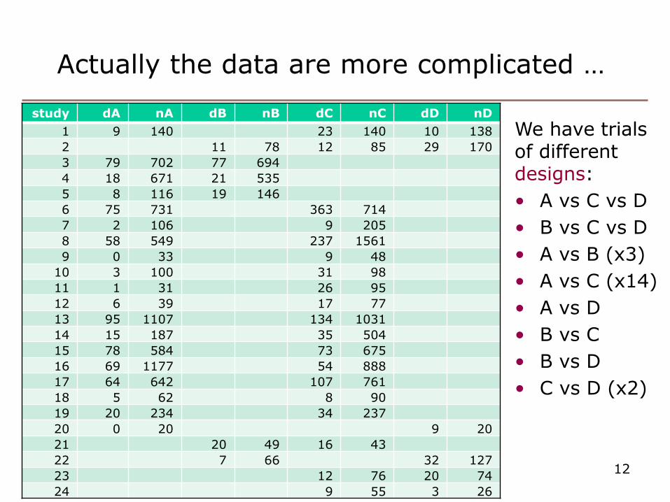
Actually the data are more complicated …
12
We have trials of different designs:
• A vs C vs D
• B vs C vs D
• A vs B (x3)
• A vs C (x14)
• A vs D
• B vs C
• B vs D
• C vs D (x2)
study dA nA dB nB dC nC dD nD
1 9 140 23 140 10 138
2 11 78 12 85 29 170
3 79 702 77 694
4 18 671 21 535
5 8 116 19 146
6 75 731 363 714
7 2 106 9 205
8 58 549 237 1561
9 0 33 9 48
10 3 100 31 98
11 1 31 26 95
12 6 39 17 77
13 95 1107 134 1031
14 15 187 35 504
15 78 584 73 675
16 69 1177 54 888
17 64 642 107 761
18 5 62 8 90
19 20 234 34 237
20 0 20 9 20
21 20 49 16 43
22 7 66 32 127
23 12 76 20 74
24 9 55 3 26
13
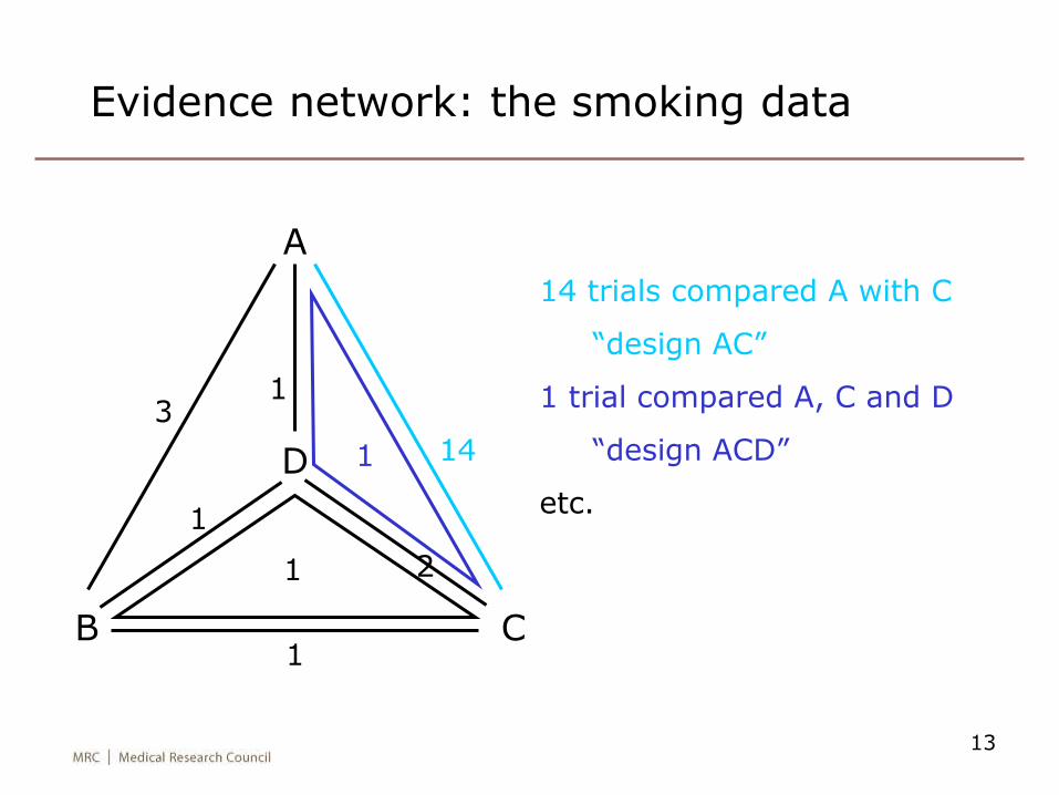
Evidence network: the smoking data
A
CB
D
3
1
1 14
1
1
1
2
14 trials compared A with C
“design AC”
1 trial compared A, C and D
“design ACD”
etc.
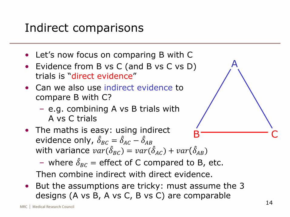
Indirect comparisons
• Let’s now focus on comparing B with C
• Evidence from B vs C (and B vs C vs D)trials is “direct evidence”
• Can we also use indirect evidence to compare B with C?
– e.g. combining A vs B trials with A vs C trials
• The maths is easy: using indirect
evidence only, 𝛿𝐵𝐶 = 𝛿𝐴𝐶 − 𝛿𝐴𝐵
with variance 𝑣𝑎𝑟( 𝛿𝐵𝐶) = 𝑣𝑎𝑟( 𝛿𝐴𝐶) + 𝑣𝑎𝑟( 𝛿𝐴𝐵)
– where 𝛿𝐵𝐶 = effect of C compared to B, etc.
Then combine indirect with direct evidence.
• But the assumptions are tricky: must assume the 3 designs (A vs B, A vs C, B vs C) are comparable
14
A
CB
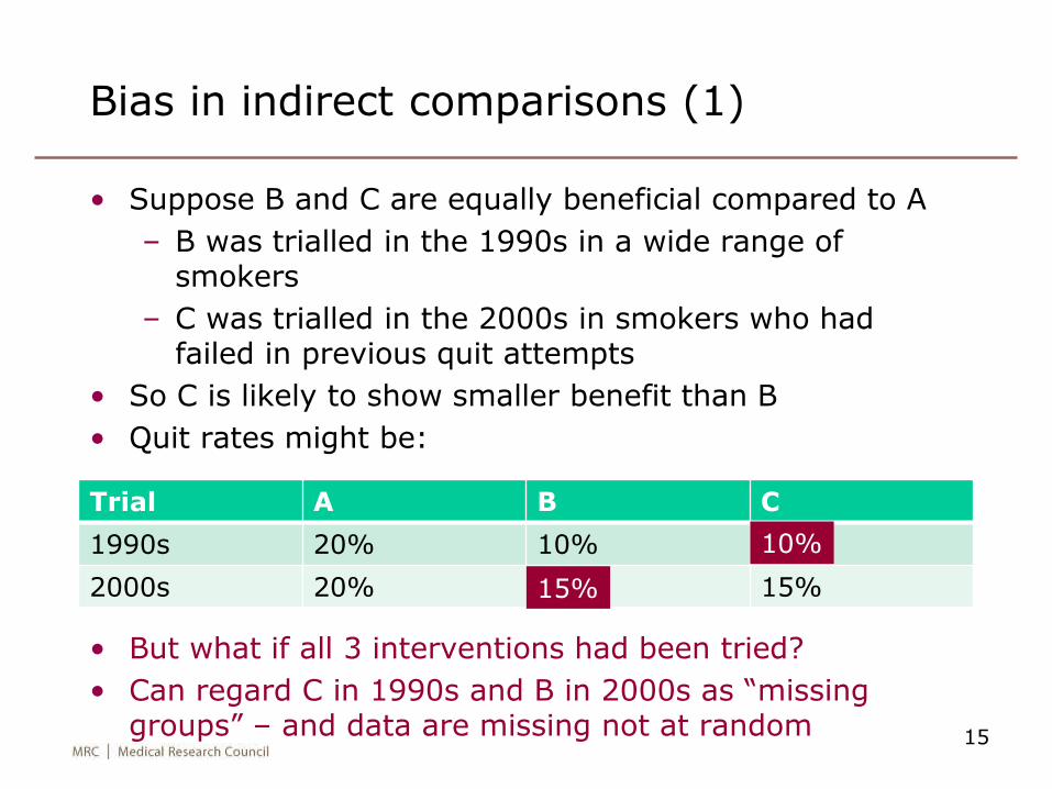
Bias in indirect comparisons (1)
• Suppose B and C are equally beneficial compared to A
– B was trialled in the 1990s in a wide range of smokers
– C was trialled in the 2000s in smokers who had failed in previous quit attempts
• So C is likely to show smaller benefit than B
• Quit rates might be:
• But what if all 3 interventions had been tried?
• Can regard C in 1990s and B in 2000s as “missing groups” – and data are missing not at random 15
Trial A B C
1990s 20% 10%
2000s 20% 15%
10%
15%
Smoking quit rates
Trial A B C
A vs. B 20% 10%
A vs. C 10% 3%
Comparison with A
Risk difference
Risk ratio
Odds ratio
-10% 0.5 0.44
-7% 0.3 0.28
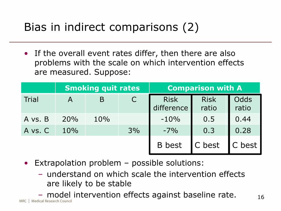
Bias in indirect comparisons (2)
• If the overall event rates differ, then there are also problems with the scale on which intervention effects are measured. Suppose:
16
B best C best C best
• Extrapolation problem – possible solutions:
– understand on which scale the intervention effects are likely to be stable
– model intervention effects against baseline rate.
Network meta-analysis
• Despite these problems, I’ll proceed to combine all the evidence – indirect and direct – in order to get our best estimates of the value of all the interventions
• This is called network meta-analysis
– multiple treatments meta-analysis
– mixed treatment comparisons
• Network meta-analysis addresses the real clinical question: which intervention is best for the patient?
– may additionally require modelling covariates
• Much used by NICE (National Institute for Clinical Excellence) in comparing interventions
• See e.g. Salanti G, Higgins JP, Ades A, Ioannidis JP. Evaluation of networks of randomized trials. Statistical Methods in Medical Research 2008; 17: 279–301.
17
18
Aims of network meta-analysis
1. Use all the data & thus get
– better estimates of treatment effects
– opportunity to identify the best treatment
2. Assess whether the evidence is consistent
– i.e. does the indirect evidence agree with the direct evidence?
The main statistical challenges are
– formulating and fitting models that allow for heterogeneity and inconsistency
– assessing inconsistency and (if found) finding ways to handle it
Less-statistical challenges include defining the scope of the problem: which treatments to include, what patient groups, what outcomes
19
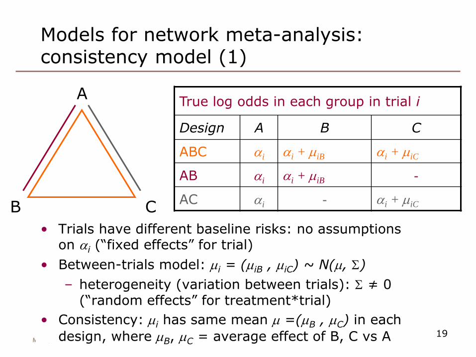
Models for network meta-analysis: consistency model (1)
True log odds in each group in trial i
Design A B C
ABC ai ai + miB ai + miC
AB ai ai + miB -
AC ai - ai + miC
A
CB
• Trials have different baseline risks: no assumptions on ai (“fixed effects” for trial)
• Between-trials model: mi = (miB , miC) ~ N(m, S)
– heterogeneity (variation between trials): S ≠ 0(“random effects” for treatment*trial)
• Consistency: mi has same mean m =(mB , mC) in each
design, where mB, mC = average effect of B, C vs A
20
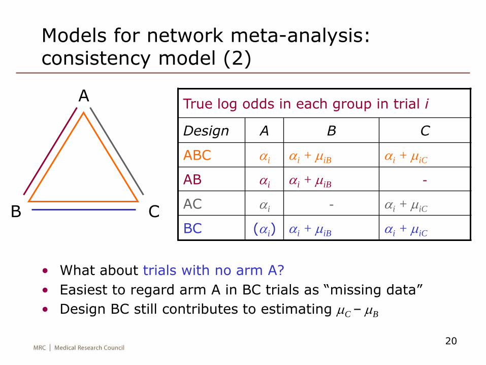
• What about trials with no arm A?
• Easiest to regard arm A in BC trials as “missing data”
• Design BC still contributes to estimating mC – mB
Models for network meta-analysis: consistency model (2)
True log odds in each group in trial i
Design A B C
ABC ai ai + miB ai + miC
AB ai ai + miB -
AC ai - ai + miC
BC (ai) ai + miB ai + miC
A
CB
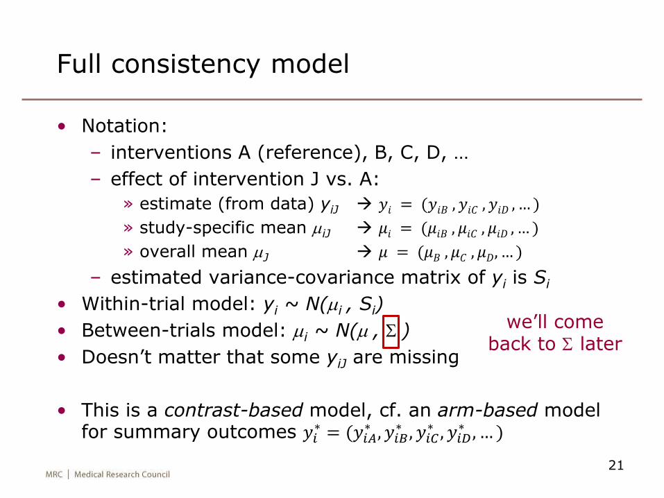
Full consistency model
• Notation:
– interventions A (reference), B, C, D, …
– effect of intervention J vs. A:
» estimate (from data) yiJ 𝑦𝑖 = (𝑦𝑖𝐵 , 𝑦𝑖𝐶 , 𝑦𝑖𝐷 , … )
» study-specific mean miJ 𝜇𝑖 = (𝜇𝑖𝐵 , 𝜇𝑖𝐶 , 𝜇𝑖𝐷 , … )
» overall mean mJ 𝜇 = (𝜇𝐵 , 𝜇𝐶 , 𝜇𝐷, … )
– estimated variance-covariance matrix of yi is Si
• Within-trial model: yi ~ N(mi , Si)
• Between-trials model: mi ~ N(m , S )
• Doesn’t matter that some yiJ are missing
• This is a contrast-based model, cf. an arm-based model for summary outcomes 𝑦𝑖
∗ = (𝑦𝑖𝐴∗ , 𝑦𝑖𝐵
∗ , 𝑦𝑖𝐶∗ , 𝑦𝑖𝐷
∗ , … )
21
we’ll come back to S later
Inconsistency models
• Lu & Ades (2006)
• Node-splitting (Dias et al 2010)– Dias S, Welton NJ, Caldwell DM, Ades AE. Checking consistency in
mixed treatment comparison meta-analysis. Statistics in Medicine2010; 29: 932–944.
• Design-by-treatment interaction (Higgins et al 2012)– Higgins JPT, Jackson D, Barrett JL, Lu G, Ades AE, White IR.
Consistency and inconsistency in network meta-analysis: concepts and models for multi-arm studies. Research Synthesis Methods2012; 3: 98–110.
22
23
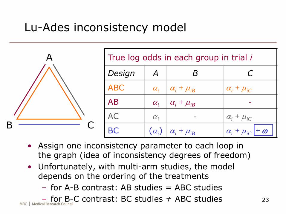
Lu-Ades inconsistency model
True log odds in each group in trial i
Design A B C
ABC ai ai + miB ai + miC
AB ai ai + miB -
AC ai - ai + miC
BC (ai) ai + miB ai + miC + w
A
CB
• Assign one inconsistency parameter to each loop in the graph (idea of inconsistency degrees of freedom)
• Unfortunately, with multi-arm studies, the model depends on the ordering of the treatments
– for A-B contrast: AB studies = ABC studies
– for B-C contrast: BC studies ≠ ABC studies
24
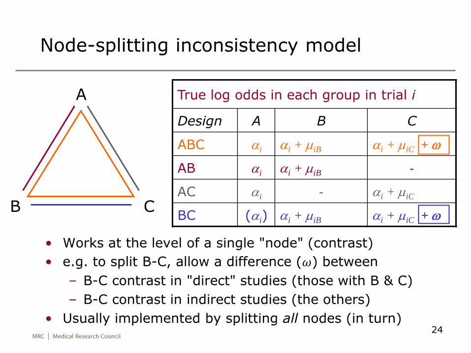
Node-splitting inconsistency model
True log odds in each group in trial i
Design A B C
ABC ai ai + miB ai + miC + w
AB ai ai + miB -
AC ai - ai + miC
BC (ai) ai + miB ai + miC + w
A
CB
• Works at the level of a single "node" (contrast)
• e.g. to split B-C, allow a difference (𝜔) between
– B-C contrast in "direct" studies (those with B & C)
– B-C contrast in indirect studies (the others)
• Usually implemented by splitting all nodes (in turn)
25
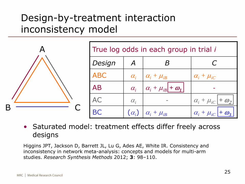
Design-by-treatment interaction inconsistency model
True log odds in each group in trial i
Design A B C
ABC ai ai + miB ai + miC
AB ai ai + miB + w1 -
AC ai - ai + miC + w2
BC (ai) ai + miB ai + miC + w3
A
CB
• Saturated model: treatment effects differ freely across designs
Higgins JPT, Jackson D, Barrett JL, Lu G, Ades AE, White IR. Consistency and inconsistency in network meta-analysis: concepts and models for multi-arm studies. Research Synthesis Methods 2012; 3: 98–110.
Comparison of inconsistency models
• The design-by-treatment interaction model
– contains all the Lu-Ades and node-splitting models
– is the union of all node-splitting models (we think)
– so is the best model for a global test of inconsistency
• Node-splitting model is most appropriate if interest lies in a particular comparison
26
Fixed or random inconsistency?
The Lu-Ades and design-by-treatment interaction models have several inconsistency parameters. We can take these as
• Fixed effects
– easier for interpretation of the inconsistency parameters
– easier for testing consistency
• Random effects
– makes the overall mean interpretable as an average treatment effect over the inconsistency distribution (Jackson et al, 2014)
Here I take them as fixed effects.
[NB distinguish "fixed effects" (𝜔's all separate) from "fixed-effect" (true treatment effects 𝜇𝑖 all equal)]
27
Heterogeneity
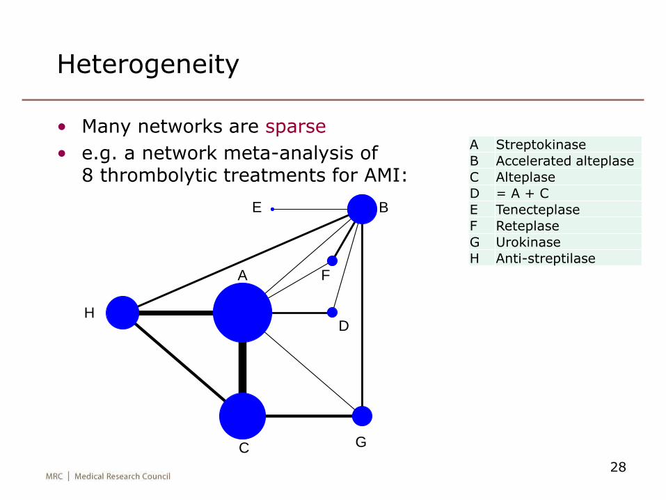
• Many networks are sparse
• e.g. a network meta-analysis of8 thrombolytic treatments for AMI:
28
A Streptokinase
B Accelerated alteplase
C Alteplase
D = A + C
E Tenecteplase
F Reteplase
G Urokinase
H Anti-streptilase
A
B
C
D
E
F
G
H
Heterogeneity models
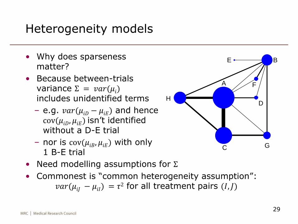
• Why does sparseness matter?
• Because between-trials variance Σ = 𝑣𝑎𝑟(𝜇𝑖)includes unidentified terms
– e.g. 𝑣𝑎𝑟(𝜇𝑖𝐷 − 𝜇𝑖𝐸) and hence cov(𝜇𝑖𝐷, 𝜇𝑖𝐸) isn’t identified without a D-E trial
– nor is cov(𝜇𝑖𝐵, 𝜇𝑖𝐸) with only 1 B-E trial
• Need modelling assumptions for Σ
• Commonest is “common heterogeneity assumption”:𝑣𝑎𝑟(𝜇𝑖𝐽 − 𝜇𝑖𝐼) = 𝜏2 for all treatment pairs (𝐼, 𝐽)
29
A
B
C
D
E
F
G
H
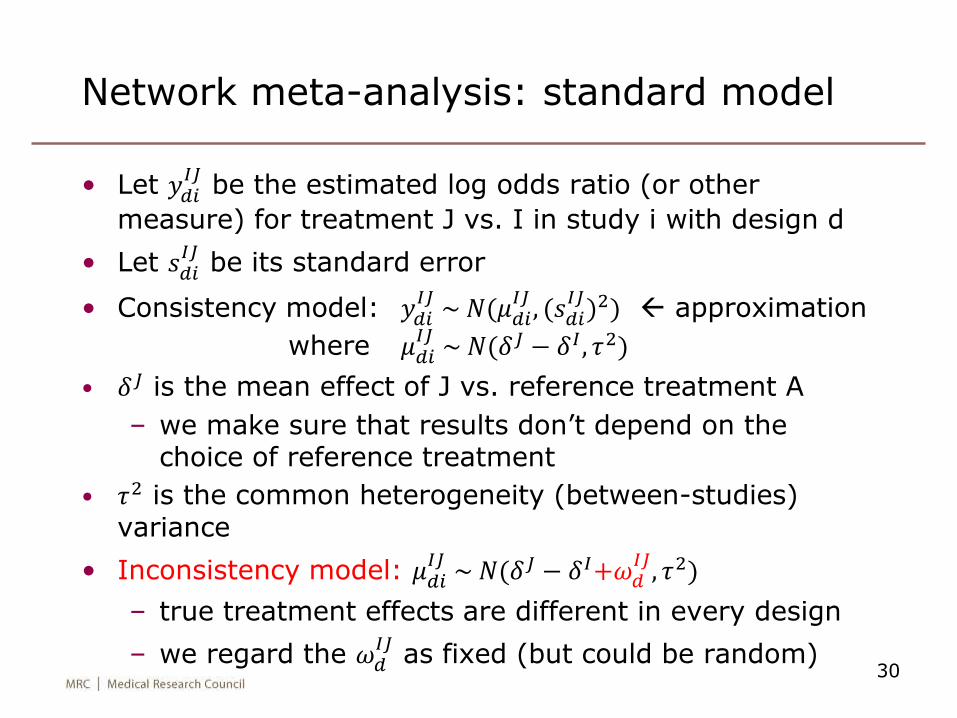
Network meta-analysis: standard model
• Let 𝑦𝑑𝑖𝐼𝐽
be the estimated log odds ratio (or other
measure) for treatment J vs. I in study i with design d
• Let 𝑠𝑑𝑖𝐼𝐽
be its standard error
• Consistency model: 𝑦𝑑𝑖𝐼𝐽
~ 𝑁(𝜇𝑑𝑖𝐼𝐽
, (𝑠𝑑𝑖𝐼𝐽
)2) approximation
where 𝜇𝑑𝑖𝐼𝐽
~ 𝑁(𝛿𝐽 − 𝛿𝐼 , 𝜏2)
• 𝛿𝐽 is the mean effect of J vs. reference treatment A
– we make sure that results don’t depend on the choice of reference treatment
• 𝜏2 is the common heterogeneity (between-studies) variance
• Inconsistency model: 𝜇𝑑𝑖𝐼𝐽
~ 𝑁(𝛿𝐽 − 𝛿𝐼+𝜔𝑑𝐼𝐽
, 𝜏2)
– true treatment effects are different in every design
– we regard the 𝜔𝑑𝐼𝐽
as fixed (but could be random)30
Network meta-analyses: estimation
• In the past, the models have been fitted using WinBUGS
– because frequentist alternatives have not been available
– has made network meta-analysis difficult for non-statisticians
• Now, consistency and inconsistency models can be fitted using multivariate meta-analysis and multivariate meta-regression
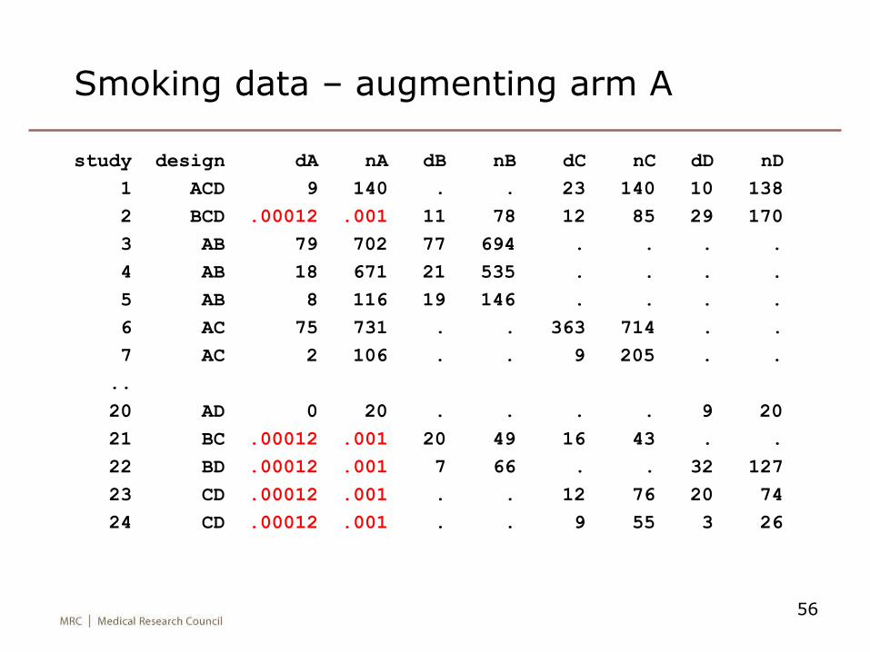
• Trials without the reference intervention are handled
– by a trial-specific baseline intervention (complicates code); or
– by “augmenting” these trials with a very small reference arm (e.g. 0.0001 successes out of 0.001)
31
Network meta-analysis: multi-arm trials
• Multi-arm trials contribute >1 log odds ratio
– need to allow for their covariance
– mathematically straightforward but complicates programming
• With only 2-arm trials, we can fit models using standard “meta-regression”
• Multi-arm trials complicate this – need suitable data formats and multivariate analysis
32
Example analyses
33
34
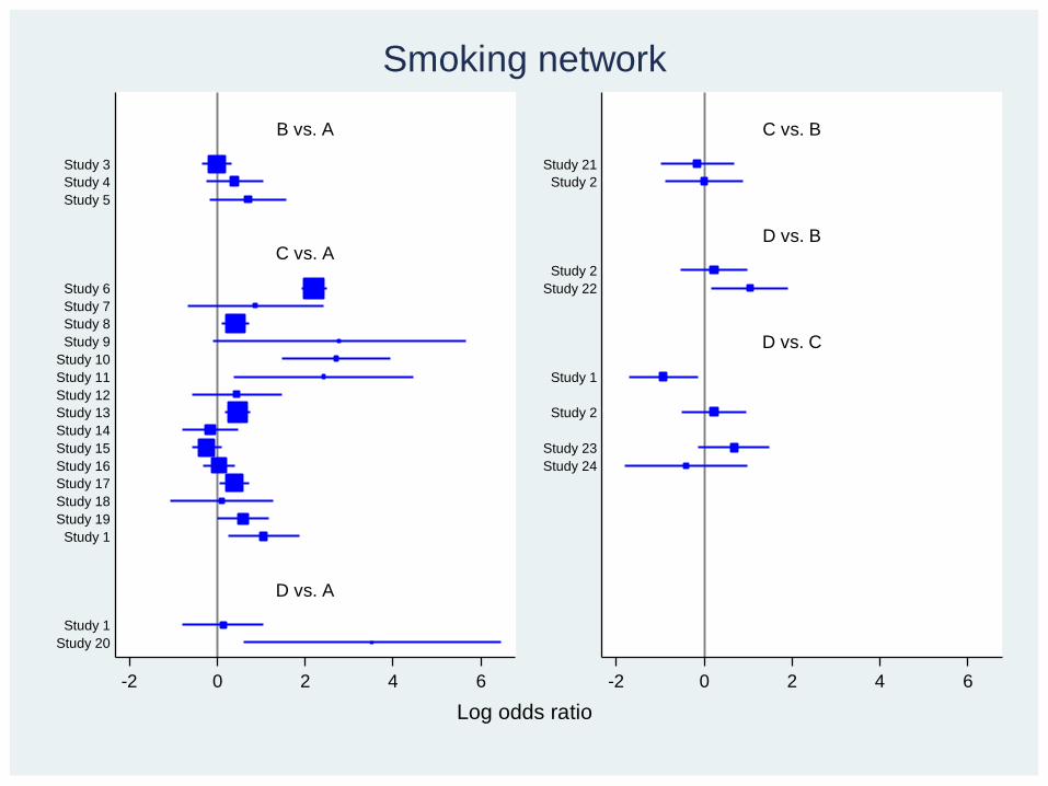
B vs. A
C vs. A
D vs. A
C vs. B
D vs. B
D vs. C
Study 3
Study 4
Study 5
Study 6
Study 7
Study 8
Study 9
Study 10
Study 11
Study 12
Study 13
Study 14
Study 15
Study 16
Study 17
Study 18
Study 19
Study 1
Study 1
Study 20
Study 21
Study 2
Study 2
Study 22
Study 1
Study 2
Study 23
Study 24
-2 0 2 4 6 -2 0 2 4 6
Log odds ratio
Smoking network
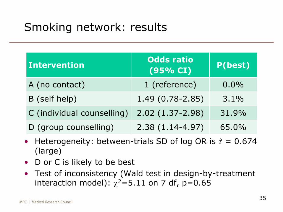
Smoking network: results
• Heterogeneity: between-trials SD of log OR is 𝜏 = 0.674 (large)
• D or C is likely to be best
• Test of inconsistency (Wald test in design-by-treatment interaction model): c2=5.11 on 7 df, p=0.65
35
InterventionOdds ratio
(95% CI)P(best)
A (no contact) 1 (reference) 0.0%
B (self help) 1.49 (0.78-2.85) 3.1%
C (individual counselling) 2.02 (1.37-2.98) 31.9%
D (group counselling) 2.38 (1.14-4.97) 65.0%
36
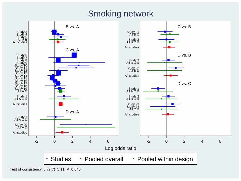
B vs. A
C vs. A
D vs. A
C vs. B
D vs. B
D vs. C
Study 3Study 4Study 5All A B
All studies
Study 6Study 7Study 8Study 9
Study 10Study 11Study 12Study 13Study 14Study 15Study 16Study 17Study 18Study 19
All A C
Study 1All A C D
All studies
Study 1All A C D
Study 20
All A D
All studies
Study 21All B C
Study 2
All B C D
All studies
Study 2All B C D
Study 22
All B D
All studies
Study 1All A C D
Study 2
All B C D
Study 23Study 24
All C D
All studies
-2 0 2 4 6 -2 0 2 4 6
Studies Pooled overall Pooled within design
Log odds ratio
Test of consistency: chi2(7)=5.11, P=0.646
Smoking network
37
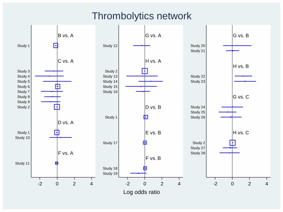
B vs. A
C vs. A
D vs. A
F vs. A
G vs. A
H vs. A
D vs. B
E vs. B
F vs. B
G vs. B
H vs. B
G vs. C
H vs. C
Study 1
Study 3
Study 4
Study 5
Study 6
Study 7
Study 8
Study 9
Study 2
Study 1
Study 10
Study 11
Study 12
Study 2
Study 13
Study 14
Study 15
Study 16
Study 1
Study 17
Study 18
Study 19
Study 20
Study 21
Study 22
Study 23
Study 24
Study 25
Study 26
Study 2
Study 27
Study 28
-2 0 2 4 -2 0 2 4 -2 0 2 4
Log odds ratio
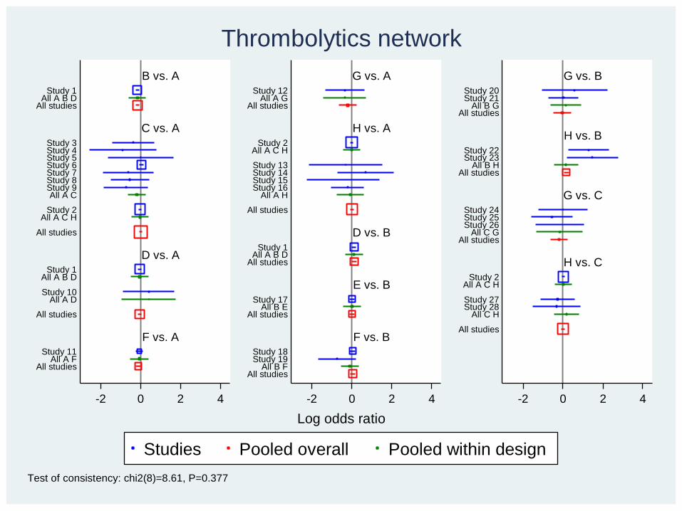
Thrombolytics network
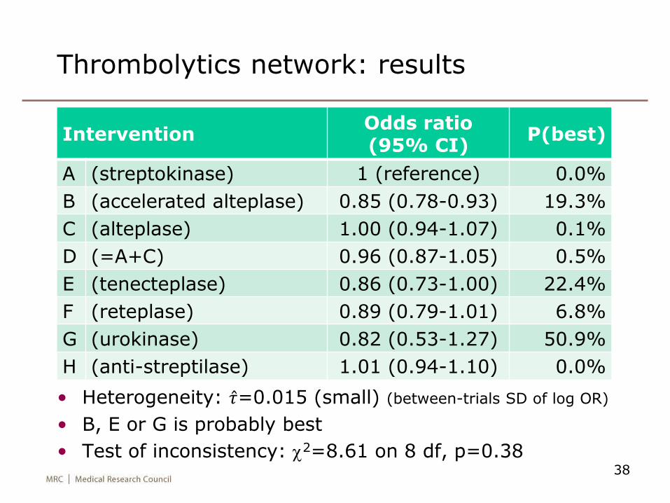
Thrombolytics network: results
• Heterogeneity: 𝜏=0.015 (small) (between-trials SD of log OR)
• B, E or G is probably best
• Test of inconsistency: c2=8.61 on 8 df, p=0.3838
InterventionOdds ratio(95% CI)
P(best)
A (streptokinase) 1 (reference) 0.0%
B (accelerated alteplase) 0.85 (0.78-0.93) 19.3%
C (alteplase) 1.00 (0.94-1.07) 0.1%
D (=A+C) 0.96 (0.87-1.05) 0.5%
E (tenecteplase) 0.86 (0.73-1.00) 22.4%
F (reteplase) 0.89 (0.79-1.01) 6.8%
G (urokinase) 0.82 (0.53-1.27) 50.9%
H (anti-streptilase) 1.01 (0.94-1.10) 0.0%
39
B vs. A
C vs. A
D vs. A
F vs. A
G vs. A
H vs. A
D vs. B
E vs. B
F vs. B
G vs. B
H vs. B
G vs. C
H vs. C
Study 1All A B D
All studies
Study 3Study 4Study 5Study 6Study 7Study 8Study 9All A C
Study 2
All A C H
All studies
Study 1All A B D
Study 10
All A D
All studies
Study 11All A F
All studies
Study 12All A G
All studies
Study 2All A C H
Study 13Study 14Study 15Study 16
All A H
All studies
Study 1All A B D
All studies
Study 17All B E
All studies
Study 18Study 19
All B FAll studies
Study 20Study 21
All B GAll studies
Study 22Study 23
All B HAll studies
Study 24Study 25Study 26
All C GAll studies
Study 2All A C H
Study 27Study 28
All C H
All studies
-2 0 2 4 -2 0 2 4 -2 0 2 4
Studies Pooled overall Pooled within design
Log odds ratio
Test of consistency: chi2(8)=8.61, P=0.377
Thrombolytics network
Some controversies
40
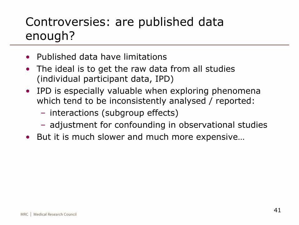
Controversies: are published data enough?
• Published data have limitations
• The ideal is to get the raw data from all studies (individual participant data, IPD)
• IPD is especially valuable when exploring phenomena which tend to be inconsistently analysed / reported:
– interactions (subgroup effects)
– adjustment for confounding in observational studies
• But it is much slower and much more expensive…
41
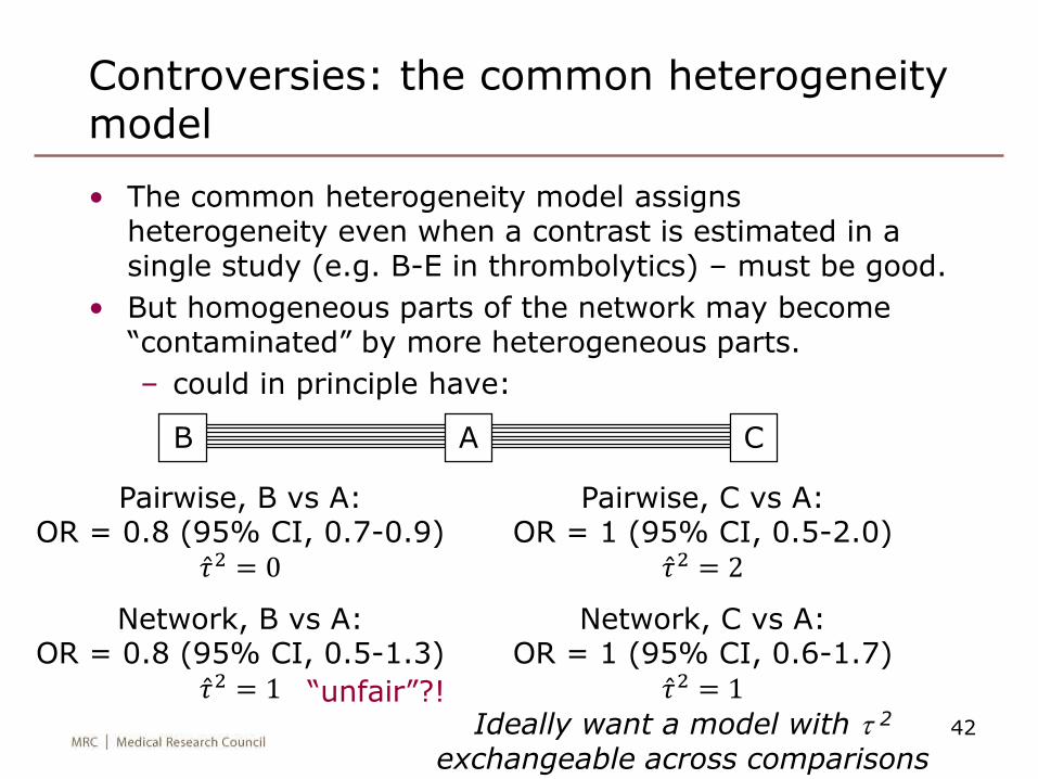
Controversies: the common heterogeneity model
• The common heterogeneity model assigns heterogeneity even when a contrast is estimated in a single study (e.g. B-E in thrombolytics) – must be good.
• But homogeneous parts of the network may become “contaminated” by more heterogeneous parts.
– could in principle have:
42
CAB
Pairwise, B vs A:OR = 0.8 (95% CI, 0.7-0.9)
𝜏2 = 0
Network, B vs A:OR = 0.8 (95% CI, 0.5-1.3)
𝜏2 = 1
Pairwise, C vs A:OR = 1 (95% CI, 0.5-2.0)
𝜏2 = 2
Network, C vs A:OR = 1 (95% CI, 0.6-1.7)
𝜏2 = 1“unfair”?!Ideally want a model with t 2
exchangeable across comparisons
Controversies: testing for inconsistency
• Test for inconsistency is a global test on many degrees of freedom
– likely to have low power in practice
• Can we use substantive knowledge to define more targetted tests?
• Should we accept that inconsistency is present even when test is non-significant?
43
Controversies: allowing for inconsistency
What do we do if we decide we have inconsistency?
Obviously we first try to explain it – “did the A-B trials recruit more severely ill patients?”, etc.
If we fail, then do we
• refuse to draw conclusions about treatment comparisons? (maybe we asked the wrong question?)
• infer treatment comparisons from the consistency model, with appropriate caveats?
• treat inconsistency as another random effect?
– we’ve proposed a model for this (Jackson et al, under review)
– it inflates std errors to “account for” inconsistency
– just as the standard random-effects model inflates std errors to “account for” heterogeneity.
44
Controversies: estimation
• Network meta-analysis was in the past done using Bayesian methods (1-stage analysis, arm-based model, full binomial likelihood)
– WinBUGS
– rank treatments, give p(treatment C is best) etc.
• I’ve proposed frequentist methods based on multivariate meta-analysis (2-stage analysis, contrast-based model, Normal approximation to the likelihood)
– faster and more accessible
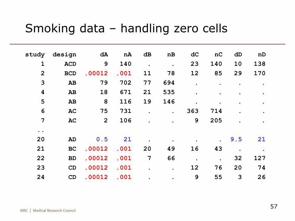
– don’t allow well for sparse binary data (e.g. smoking trial 9: 0/33 vs 9/48)
• Next slide compares the methods in the smoking data…
45
46
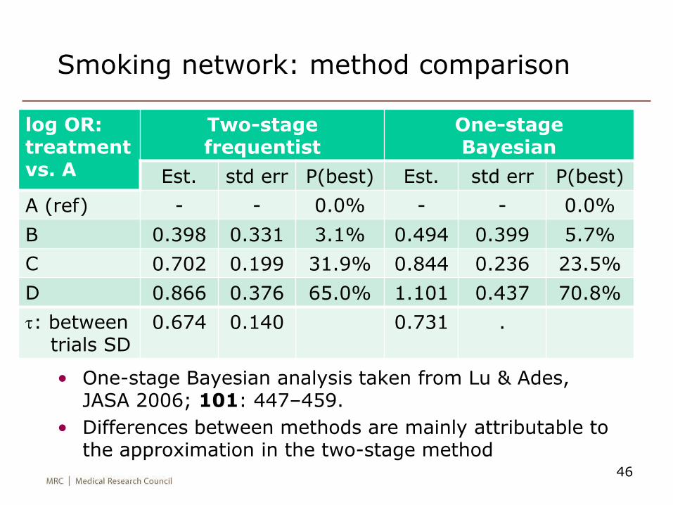
Smoking network: method comparison
log OR: treatment vs. A
Two-stage frequentist
One-stage Bayesian
Est. std err P(best) Est. std err P(best)
A (ref) - - 0.0% - - 0.0%
B 0.398 0.331 3.1% 0.494 0.399 5.7%
C 0.702 0.199 31.9% 0.844 0.236 23.5%
D 0.866 0.376 65.0% 1.101 0.437 70.8%
t: between trials SD
0.674 0.140 0.731 .
• One-stage Bayesian analysis taken from Lu & Ades, JASA 2006; 101: 447–459.
• Differences between methods are mainly attributable to the approximation in the two-stage method
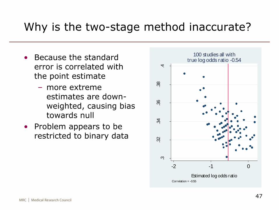
Why is the two-stage method inaccurate?
• Because the standard error is correlated with the point estimate
– more extreme estimates are down-weighted, causing bias towards null
• Problem appears to be restricted to binary data
47
.3.3
2.3
4.3
6.3
8.4
Stan
dar
d e
rror
of est
imat
ed log
odds
rati
o
-2 -1 0
Estimated log odds ratio
Correlation = -0.55
100 studies all withtrue log odds ratio -0.54
A frequentist one-stage method for binary data?
• Should be able to fit a generalised linear mixed model (Stata melogit)
– random effect for study*treatment interaction
– (± fixed or random effect for design*treatment interaction)
• How do we handle main effect of study?
– fixed effect? one parameter per study may underestimate heterogeneity variance & std error
– random effect? but then results are contaminated by between-study information
– eliminate it by conditioning on study margins? may be ideal but computationally difficultStijnen T, Hamza TH, Özdemir P. Random effects meta-analysis of event outcome in the framework of the generalized linear mixed model with applications in sparse data. Statistics in Medicine 2010; 29: 3046–3067.
48
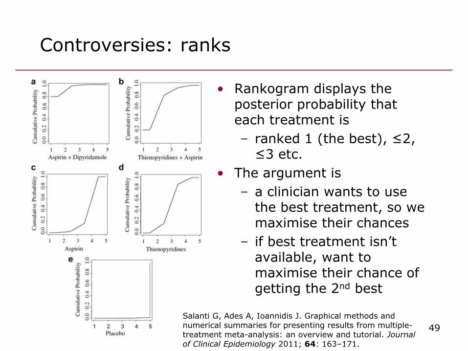
Controversies: ranks
• Rankogram displays the posterior probability that each treatment is
– ranked 1 (the best), ≤2, ≤3 etc.
• The argument is
– a clinician wants to use the best treatment, so we maximise their chances
– if best treatment isn’t available, want to maximise their chance of getting the 2nd best
49
Salanti G, Ades A, Ioannidis J. Graphical methods and numerical summaries for presenting results from multiple-treatment meta-analysis: an overview and tutorial. Journal of Clinical Epidemiology 2011; 64: 163–171.
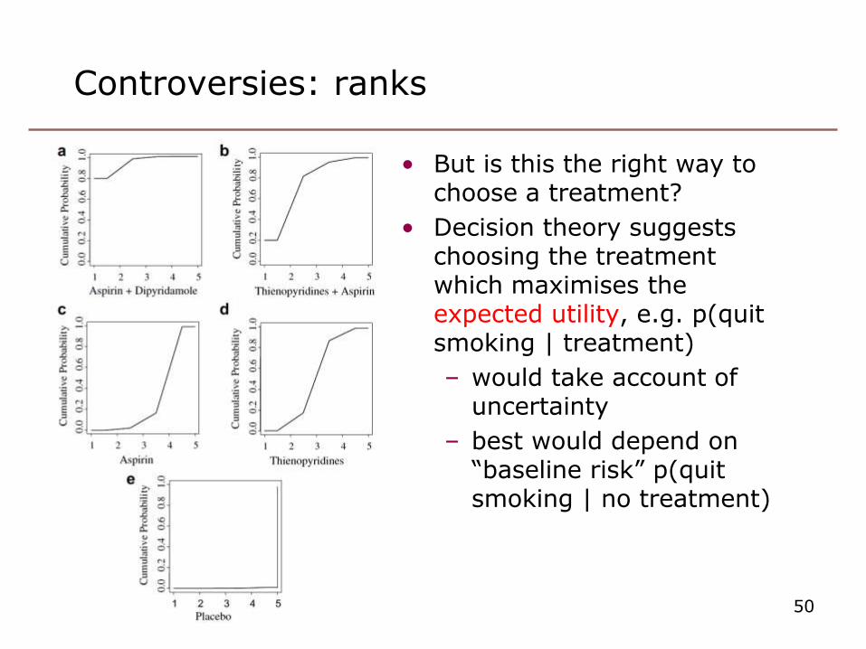
Controversies: ranks
• But is this the right way to choose a treatment?
• Decision theory suggests choosing the treatment which maximises the expected utility, e.g. p(quit smoking | treatment)
– would take account of uncertainty
– best would depend on “baseline risk” p(quit smoking | no treatment)
50
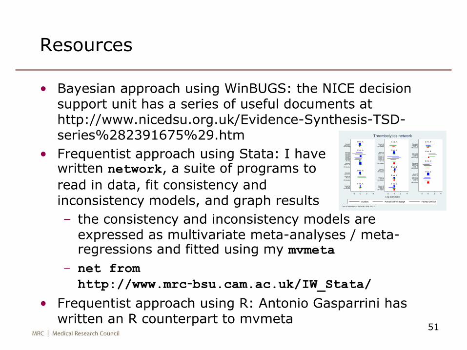
Resources
• Bayesian approach using WinBUGS: the NICE decision support unit has a series of useful documents at http://www.nicedsu.org.uk/Evidence-Synthesis-TSD-series%282391675%29.htm
• Frequentist approach using Stata: I havewritten network, a suite of programs to
read in data, fit consistency andinconsistency models, and graph results
– the consistency and inconsistency models are expressed as multivariate meta-analyses / meta-regressions and fitted using my mvmeta
– net from
http://www.mrc-bsu.cam.ac.uk/IW_Stata/
• Frequentist approach using R: Antonio Gasparrini has written an R counterpart to mvmeta
51
B vs. A
C vs. A
D vs. A
F vs. A
G vs. A
H vs. A
D vs. B
E vs. B
F vs. B
G vs. B
H vs. B
G vs. C
H vs. C
Study 1All A B D
All studies
Study 3Study 4Study 5Study 6Study 7Study 8Study 9All A C
Study 2
All A C H
All studies
Study 1All A B D
Study 10
All A D
All studies
Study 11All A F
All studies
Study 12All A G
All studies
Study 2All A C H
Study 13Study 14Study 15Study 16
All A H
All studies
Study 1All A B D
All studies
Study 17All B E
All studies
Study 18Study 19
All B FAll studies
Study 20Study 21
All B GAll studies
Study 22Study 23
All B HAll studies
Study 24Study 25Study 26
All C GAll studies
Study 2All A C H
Study 27Study 28
All C H
All studies
-2 0 2 4 -2 0 2 4 -2 0 2 4
Studies Pooled within design Pooled overall
Log odds ratio
Test of consistency: chi2=8.61, df=8, P=0.377
Thrombolytics network
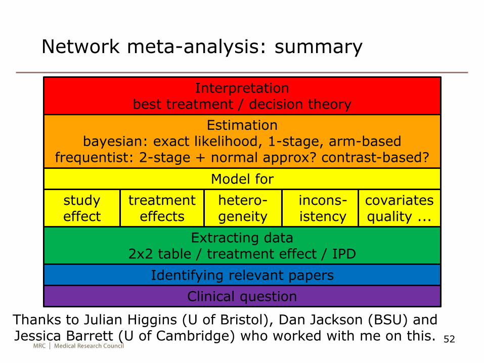
Network meta-analysis: summary
52
Clinical question
Identifying relevant papers
Extracting data2x2 table / treatment effect / IPD
Model for
studyeffect
treatment effects
hetero-geneity
incons-istency
covariates quality ...
Estimationbayesian: exact likelihood, 1-stage, arm-based
frequentist: 2-stage + normal approx? contrast-based?
Interpretationbest treatment / decision theory
Thanks to Julian Higgins (U of Bristol), Dan Jackson (BSU) and Jessica Barrett (U of Cambridge) who worked with me on this.

Extra slides
53
54
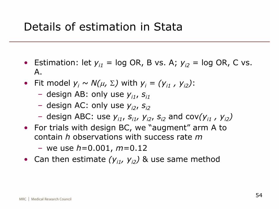
Details of estimation in Stata
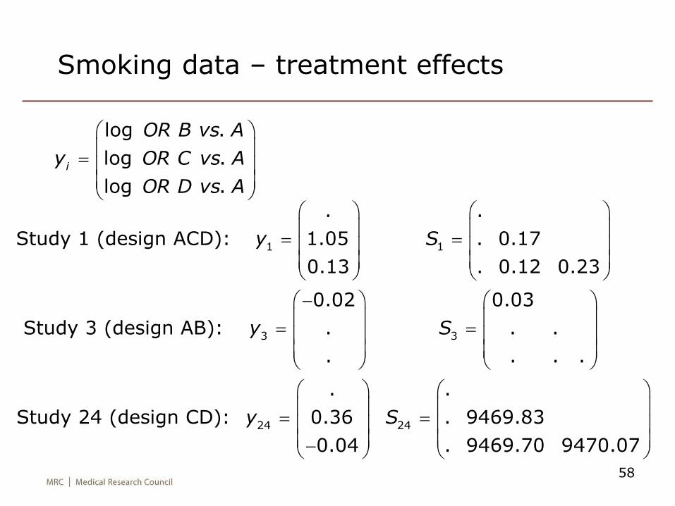
• Estimation: let yi1 = log OR, B vs. A; yi2 = log OR, C vs. A.
• Fit model yi ~ N(m, S) with yi = (yi1 , yi2):
– design AB: only use yi1, si1
– design AC: only use yi2, si2
– design ABC: use yi1, si1, yi2, si2 and cov(yi1 , yi2)
• For trials with design BC, we “augment” arm A to contain h observations with success rate m
– we use h=0.001, m=0.12
• Can then estimate (yi1, yi2) & use same method
55
Smoking data
study design dA nA dB nB dC nC dD nD
1 ACD 9 140 . . 23 140 10 138
2 BCD . . 11 78 12 85 29 170
3 AB 79 702 77 694 . . . .
4 AB 18 671 21 535 . . . .
5 AB 8 116 19 146 . . . .
6 AC 75 731 . . 363 714 . .
7 AC 2 106 . . 9 205 . .
..
20 AD 0 20 . . . . 9 20
21 BC . . 20 49 16 43 . .
22 BD . . 7 66 . . 32 127
23 CD . . . . 12 76 20 74
24 CD . . . . 9 55 3 26
successes and participants in arm D
56
Smoking data – augmenting arm A
study design dA nA dB nB dC nC dD nD
1 ACD 9 140 . . 23 140 10 138
2 BCD .00012 .001 11 78 12 85 29 170
3 AB 79 702 77 694 . . . .
4 AB 18 671 21 535 . . . .
5 AB 8 116 19 146 . . . .
6 AC 75 731 . . 363 714 . .
7 AC 2 106 . . 9 205 . .
..
20 AD 0 20 . . . . 9 20
21 BC .00012 .001 20 49 16 43 . .
22 BD .00012 .001 7 66 . . 32 127
23 CD .00012 .001 . . 12 76 20 74
24 CD .00012 .001 . . 9 55 3 26
57
Smoking data – handling zero cells
study design dA nA dB nB dC nC dD nD
1 ACD 9 140 . . 23 140 10 138
2 BCD .00012 .001 11 78 12 85 29 170
3 AB 79 702 77 694 . . . .
4 AB 18 671 21 535 . . . .
5 AB 8 116 19 146 . . . .
6 AC 75 731 . . 363 714 . .
7 AC 2 106 . . 9 205 . .
..
20 AD 0.5 21 . . . . 9.5 21
21 BC .00012 .001 20 49 16 43 . .
22 BD .00012 .001 7 66 . . 32 127
23 CD .00012 .001 . . 12 76 20 74
24 CD .00012 .001 . . 9 55 3 26
58
Smoking data – treatment effects
1 1
3 3
24 24
. .
Study 1 (design ACD): 1.05 . 0.17
0.13 . 0.12 0.23
0.02 0.03
Study 3 (design AB): . . .
. . . .
. .
Study 24 (design CD): 0.36 . 9469.83
0.04 . 9469.70 9
y S
y S
y S
470.07
log .
log .
log . i
OR B vs A
y OR C vs A
OR D vs A
59
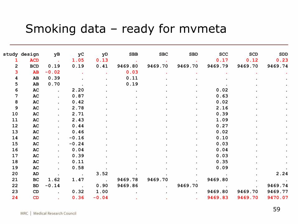
Smoking data – ready for mvmeta
study design yB yC yD SBB SBC SBD SCC SCD SDD
1 ACD . 1.05 0.13 . . . 0.17 0.12 0.23
2 BCD 0.19 0.19 0.41 9469.80 9469.70 9469.70 9469.79 9469.70 9469.74
3 AB -0.02 . . 0.03 . . . . .
4 AB 0.39 . . 0.11 . . . . .
5 AB 0.70 . . 0.19 . . . . .
6 AC . 2.20 . . . . 0.02 . .
7 AC . 0.87 . . . . 0.63 . .
8 AC . 0.42 . . . . 0.02 . .
9 AC . 2.78 . . . . 2.16 . .
10 AC . 2.71 . . . . 0.39 . .
11 AC . 2.43 . . . . 1.09 . .
12 AC . 0.44 . . . . 0.27 . .
13 AC . 0.46 . . . . 0.02 . .
14 AC . -0.16 . . . . 0.10 . .
15 AC . -0.24 . . . . 0.03 . .
16 AC . 0.04 . . . . 0.04 . .
17 AC . 0.39 . . . . 0.03 . .
18 AC . 0.11 . . . . 0.35 . .
19 AC . 0.58 . . . . 0.09 . .
20 AD . . 3.52 . . . . . 2.24
21 BC 1.62 1.47 . 9469.78 9469.70 . 9469.80 . .
22 BD -0.14 . 0.90 9469.86 . 9469.70 . . 9469.74
23 CD . 0.32 1.00 . . . 9469.80 9469.70 9469.77
24 CD . 0.36 -0.04 . . . 9469.83 9469.70 9470.07
60
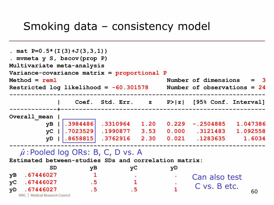
Smoking data – consistency model
. mat P=0.5*(I(3)+J(3,3,1))
. mvmeta y S, bscov(prop P)
Multivariate meta-analysis
Variance-covariance matrix = proportional P
Method = reml Number of dimensions = 3
Restricted log likelihood = -60.301578 Number of observations = 24
----------------------------------------------------------------------
| Coef. Std. Err. z P>|z| [95% Conf. Interval]
-------------+--------------------------------------------------------
Overall_mean |
yB | .3984486 .3310964 1.20 0.229 -.2504885 1.047386
yC | .7023529 .1990877 3.53 0.000 .3121483 1.092558
yD | .8658815 .3762916 2.30 0.021 .1283635 1.6034
----------------------------------------------------------------------
Estimated between-studies SDs and correlation matrix:
SD yB yC yD
yB .67446027 1 . .
yC .67446027 .5 1 .
yD .67446027 .5 .5 1
Pooled log ORs: B, C, D vs. Aˆ :m
Can also test C vs. B etc.
61
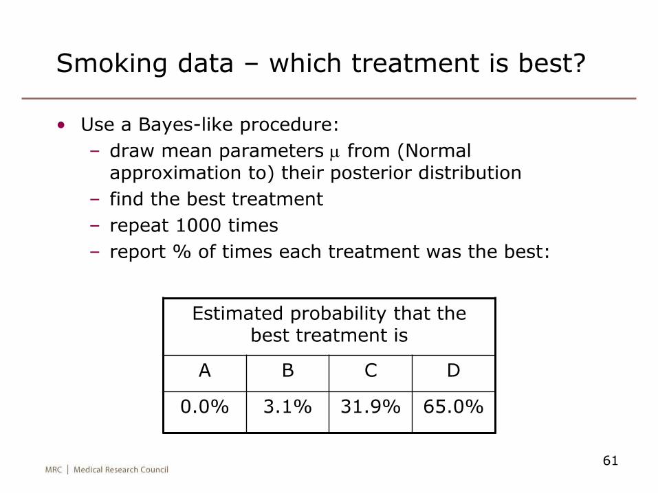
Smoking data – which treatment is best?
• Use a Bayes-like procedure:
– draw mean parameters m from (Normal approximation to) their posterior distribution
– find the best treatment
– repeat 1000 times
– report % of times each treatment was the best:
Estimated probability that the best treatment is
A B C D
0.0% 3.1% 31.9% 65.0%
62
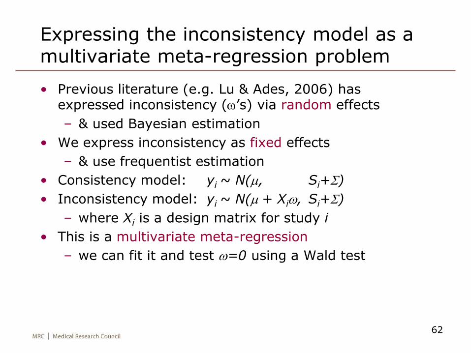
Expressing the inconsistency model as a multivariate meta-regression problem
• Previous literature (e.g. Lu & Ades, 2006) has expressed inconsistency (w’s) via random effects
– & used Bayesian estimation
• We express inconsistency as fixed effects
– & use frequentist estimation
• Consistency model: yi ~ N(m, Si+S)
• Inconsistency model: yi ~ N(m + Xiw, Si+S)
– where Xi is a design matrix for study i
• This is a multivariate meta-regression
– we can fit it and test w=0 using a Wald test
63
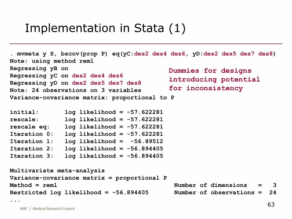
Implementation in Stata (1)
. mvmeta y S, bscov(prop P) eq(yC:des2 des4 des6, yD:des2 des5 des7 des8)
Note: using method reml
Regressing yB on
Regressing yC on des2 des4 des6
Regressing yD on des2 des5 des7 des8
Note: 24 observations on 3 variables
Variance-covariance matrix: proportional to P
initial: log likelihood = -57.622281
rescale: log likelihood = -57.622281
rescale eq: log likelihood = -57.622281
Iteration 0: log likelihood = -57.622281
Iteration 1: log likelihood = -56.89512
Iteration 2: log likelihood = -56.894405
Iteration 3: log likelihood = -56.894405
Multivariate meta-analysis
Variance-covariance matrix = proportional P
Method = reml Number of dimensions = 3
Restricted log likelihood = -56.894405 Number of observations = 24
...
Dummies for designs
introducing potential
for inconsistency
64
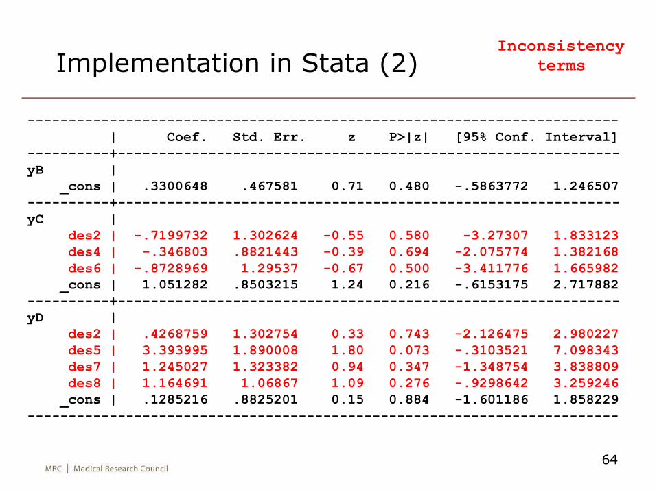
Implementation in Stata (2)
------------------------------------------------------------------------
| Coef. Std. Err. z P>|z| [95% Conf. Interval]
----------+-------------------------------------------------------------
yB |
_cons | .3300648 .467581 0.71 0.480 -.5863772 1.246507
----------+-------------------------------------------------------------
yC |
des2 | -.7199732 1.302624 -0.55 0.580 -3.27307 1.833123
des4 | -.346803 .8821443 -0.39 0.694 -2.075774 1.382168
des6 | -.8728969 1.29537 -0.67 0.500 -3.411776 1.665982
_cons | 1.051282 .8503215 1.24 0.216 -.6153175 2.717882
----------+-------------------------------------------------------------
yD |
des2 | .4268759 1.302754 0.33 0.743 -2.126475 2.980227
des5 | 3.393995 1.890008 1.80 0.073 -.3103521 7.098343
des7 | 1.245027 1.323382 0.94 0.347 -1.348754 3.838809
des8 | 1.164691 1.06867 1.09 0.276 -.9298642 3.259246
_cons | .1285216 .8825201 0.15 0.884 -1.601186 1.858229
------------------------------------------------------------------------
Inconsistency
terms
65
Implementation in Stata (3)
• Now using test we can do a Wald test of consistency
(testing the null hypothesis that all design effects = 0).
• Find c2 = 5.11 on 7 df (P=0.65)
66
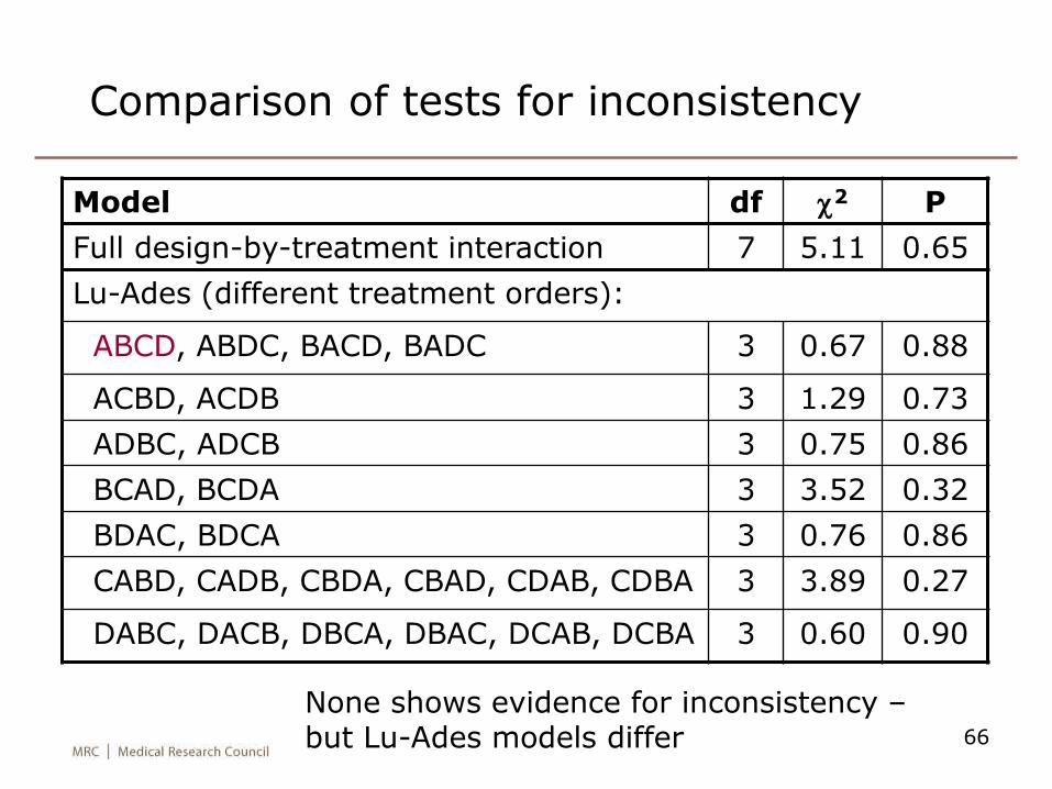
Comparison of tests for inconsistency
Model df c2 P
Full design-by-treatment interaction 7 5.11 0.65
Lu-Ades (different treatment orders):
ABCD, ABDC, BACD, BADC 3 0.67 0.88
ACBD, ACDB 3 1.29 0.73
ADBC, ADCB 3 0.75 0.86
BCAD, BCDA 3 3.52 0.32
BDAC, BDCA 3 0.76 0.86
CABD, CADB, CBDA, CBAD, CDAB, CDBA 3 3.89 0.27
DABC, DACB, DBCA, DBAC, DCAB, DCBA 3 0.60 0.90
None shows evidence for inconsistency –but Lu-Ades models differ