Inconsistency of Bayesian Inference for Misspecified ...

Bayesian Analysis (2017) 12, Number 4, pp. 1069–1103

Inconsistency of Bayesian Inferencefor Misspecified Linear Models, and a Proposal

for Repairing It

Peter Grunwald∗ and Thijs van Ommen†

Abstract. We empirically show that Bayesian inference can be inconsistent undermisspecification in simple linear regression problems, both in a model averaging/selection and in a Bayesian ridge regression setting. We use the standard lin-ear model, which assumes homoskedasticity, whereas the data are heteroskedastic(though, significantly, there are no outliers). As sample size increases, the poste-rior puts its mass on worse and worse models of ever higher dimension. This iscaused by hypercompression, the phenomenon that the posterior puts its mass ondistributions that have much larger KL divergence from the ground truth thantheir average, i.e. the Bayes predictive distribution. To remedy the problem, weequip the likelihood in Bayes’ theorem with an exponent called the learning rate,and we propose the SafeBayesian method to learn the learning rate from the data.SafeBayes tends to select small learning rates, and regularizes more, as soon ashypercompression takes place. Its results on our data are quite encouraging.

1 Introduction

We empirically demonstrate a form of inconsistency of Bayes factor model selection,model averaging and Bayesian ridge regression under model misspecification on a simplelinear regression problem with random design. We sample data (X1, Y1), (X2, Y2), . . .i.i.d. from a distribution P ∗, whereXi = (Xi1, . . . , Xipmax) are high-dimensional vectors,and we allow pmax = ∞. We use nested models M0,M1, . . . where Mp is a standardlinear model, consisting of conditional distributions P (· | β, σ2) expressing that

Yi = β0 +

p∑j=1

βjXij + εi (1)

is a linear function of p ≤ pmax covariates with additive independent Gaussian noiseεi ∼ N(0, σ2). We equip each of these models with standard priors on coefficients andthe variance, and also put a discrete prior on the models themselves. We specify a‘ground truth’ P ∗ such that M :=

⋃p=0,...,pmax

Mp does not contain the conditional

ground truth P ∗(Y | X) (hence the model is ‘misspecified’), but it does contain a P thatis ‘best’ in several respects: it is closest to P ∗ in KL (Kullback–Leibler) divergence, itrepresents the true regression function (leading to the best squared error loss predictionsamong all P ∈ M) and it has the true marginal variance (explained in Section 2.3).

∗CWI, Amsterdam and Leiden University, The Netherlands, [email protected]†University of Amsterdam, The Netherlands, [email protected]

c© 2017 International Society for Bayesian Analysis DOI: 10.1214/17-BA1085

http://bayesian.org

mailto:[email protected]

mailto:[email protected]

http://dx.doi.org/10.1214/17-BA1085

1070 Repairing Bayesian Inconsistency under Misspecification

Figure 1: The conditional expectation E[Y | X] according to the full Bayesian posteriorbased on a prior on models M0, . . . ,M50 with polynomial basis functions, given 100data points sampled i.i.d. ∼ P ∗ (about 50 of which are at (0, 0)). Standard Bayesoverfits, not as dramatically as maximum likelihood or unpenalized least squares, butstill enough to show dismal predictive behaviour as in Figure 2. In contrast, SafeBayes(which chooses learning rate η ≈ 0.4 here) and standard Bayes trained only at the pointsfor which the model is correct (not (0, 0)) both perform very well.

In fact we choose P ∗ such that P ∈ M0, and we choose our prior such that M0

receives substantial prior mass. Still, as n increases, the posterior puts most of itsmass on complex Mp’s with higher and higher p’s, and, conditional on these Mp’s, atdistributions which are very far from P ∗ both in terms of KL divergence and in terms ofL2 risk, leading to bad predictive behaviour in terms of squared error. Figures 1 and 2illustrate a particular instantiation of our results, obtained when Xij are polynomialfunctions of Si and Si ∈ [−1, 1] uniformly i.i.d. We also show comparably bad predictivebehaviour for various versions of Bayesian ridge regression, involving just a single, high-but-finite dimensional model. In that case Bayes eventually recovers and concentrateson P , but only at a sample size that is incomparably larger than what can be expectedif the model is correct.

These findings contradict the folk wisdom that, if the model is incorrect, then “Bayestends to concentrate on neighbourhoods of the distribution(s) P inM that is/are closestto P ∗ in KL divergence.” Indeed, the strongest actual theorems to this end that we knowof, (Kleijn and Van der Vaart, 2006; De Blasi and Walker, 2013; Ramamoorthi et al.,2015), hold, as the authors emphasize, under regularity conditions that are substantiallystronger than those needed for consistency when the model is correct (as by e.g. Ghosalet al. (2000) or Zhang (2006a)), and our example suggests that consistency may fail tohold even in relatively simple problems; to illustrate this further, in the supplementarymaterial (Grunwald and Van Ommen, 2017), Section G.2, we show that the regularityconditions of De Blasi and Walker (2013) are violated in our setup.

P. Grunwald and T. van Ommen 1071

Figure 2: The expected squared error risk (defined in (4)), obtained when predicting bythe full Bayesian posterior (brown curve), the SafeBayesian posterior (red curve) andthe optimal predictions (black dotted curve), as a function of sample size for the settingof Figure 1. SafeBayes is the R-log-version of SafeBayes defined in Section 4.2. Precisedefinitions and further explanation in and above Section 5.1.

How inconsistency arises The explanation for Bayes’ behaviour in our examples isillustrated in Figure 3, the essential picture to understand the phenomenon. As explainedin the text (Section 3, with a more detailed analysis in the supplementary material),the figure indicates that there exists good or ‘benign’ and bad types of misspecification.Under bad misspecification, a phenomenon we call hypercompression can take place,and that explains why at the same time we can have a good log-score of the predictivedistribution (as we must, by a result of Barron (1998)) yet a posterior that puts itsmass on very bad distributions.

The solution: Generalized and SafeBayes Bayesian updating can be enhanced witha learning rate η, an idea put forward independently by several authors (Vovk, 1990;McAllester, 2003; Barron and Cover, 1991; Walker and Hjort, 2002; Zhang, 2006a) andsuggested as a tool for dealing with misspecification by Grunwald (2011; 2012). η tradesoff the relative weight of the prior and the likelihood in determining the η-generalizedposterior, where η = 1 corresponds to standard Bayes and η = 0 means that theposterior always remains equal to the prior. When choosing the ‘right’ η, which in ourcase is significantly smaller than 1 but of course not 0, η-generalized Bayes becomescompetitive again. We give a novel interpretation of generalized Bayes in Section 4.1,showing that, for this ‘right’ η, it can be re-interpreted as standard Bayes with a differentmodel, which now has ‘good’ rather than ‘bad’ misspecification. In general, this optimalη depends on the underlying ground truth P ∗, and the remaining problem is how todetermine the optimal η empirically, from the data.

Grunwald (2012) proposed the SafeBayesian algorithm for learning η. Even thoughlacking the explicit interpretation we give in Section 4.1, he mathematically showed that


it achieves good convergence rates in terms of KL divergence on a variety of problems.1

Here we show empirically that SafeBayes performs excellently in our regression setting,being competitive with standard Bayes if the model is correct and very significantlyoutperforming standard Bayes if it is not. We do this by providing a wide range of ex-periments, varying parameters of the problem such as the priors and the true regressionfunction and studying various performance indicators such as the squared error risk,the posterior on the variance etc.

A Bayesian’s (and our) first instinct would be to learn η itself in a Bayesian manner.Yet this does not solve the problem, as we show in Section 5.4, where we consider asetting in which 1/η turns out to be exactly equivalent to the λ regularization parameterin the Bayesian Lasso and ridge regression approaches. We find that selecting η by (em-pirical) Bayes, as suggested by e.g. Park and Casella (2008), does not nearly regularizeenough in our misspecification experiments. Instead, the SafeBayesian method learnsη in a prequential fashion, finding the η which minimizes a sequential prediction erroron the data. This would still be very similar to Bayesian learning of η if the error weremeasured in terms of the standard logarithmic score, but SafeBayes, which comes intwo versions, uses a ‘randomized’ (R-log-SafeBayes) and an ‘in-model’ (I-log-SafeBayes)modification of log-score instead (Section 4.2). In the supplementary material we com-pare R- and I-log-SafeBayes to other existing methods for determining η: Section C.1provides an illuminating comparison to leave-one-out cross-validation as used in thefrequentist Lasso, and Section F briefly considers approaches from the recent Bayesianliterature Bissiri et al. (2016); Holmes and Walker (2017); Miller and Dunson (2015);Syring and Martin (2017).

The type of misspecification The models are misspecified in that they make the stan-dard assumption of homoskedasticity — σ2 is independent of X — whereas in reality,under P ∗, there is heteroskedasticity, there being a region of X with low and a regionwith (relatively) high variance. Specifically, in our simplest experiment the ‘true’ P ∗ isdefined as follows: at each i, toss a fair coin. If the coin lands heads, then sample Xi froma uniform distribution on [−1, 1], and set Yi = 0 + εi, where εi ∼ N(0, σ2

0). If the coinlands tails, then set (Xi, Yi) = (0, 0), so that there is no variance at all. The ‘best’ condi-tional density P , closest to P ∗(Y | X) in KL divergence, representing the true regressionfunction Y = 0 and moreover ‘reliable’ in the sense of Section 2.3, is then given by (1)with all β’s set to 0 and σ2 = σ2

0/2. In a typical sample of length n, we will thus haveapproximately n/2 points with Xi uniform and Yi normal with mean 0, and approxi-mately n/2 points with (Xi, Yi) = (0, 0). These points seem ‘easy’ since they lie exactlyon the regression function one would hope to learn; but they really wreak severe havoc.

Heteroskedasticity, but no outliers While it is well-known that in the presence ofoutliers, Gaussian assumptions on the noise lead to problems, both for frequentist andBayesian procedures, in the present problem we have ‘in-liers’ rather than outliers. Also,if we slightly modify the setup so that homoskedasticity holds, standard Bayes starts be-having excellently, as again depicted in Figures 1 and 2. Finally, while the figure shows

1An R package SafeBayes which implements the method for Bayesian ridge and Lasso Regression(De Heide, 2016a) is available at the Comprehensive R Archive Network (CRAN).


what happens for polynomials, we get essentially the same result with trigonometricbasis functions; in the experiments reported in this paper, we used independent mul-tivariate X’s rather than nonlinear basis functions, again getting essentially the sameresults. In the technical report (Grunwald and Van Ommen, 2014) ([GvO] from nowon) we additionally performed numerous variations on the experiments in this paper,varying priors and ground truths, and always getting qualitatively the same results. Allthis indicates that the inconsistency is really caused by misspecification, in particularthe presence of in-liers, and not by anything else. We also note that our results areentirely different from the well-known Bayesian inconsistency results of Diaconis andFreedman (1986): whereas their results are based on a well-specified model having ex-ponentially small prior mass in KL-neighbourhoods of the true P ∗, our results hold fora misspecified model, but the ‘pseudo-truth’ P can have a large prior mass (any pointmass < 1 is sufficient to get our results); see also Section B in the supplement.

Three remarks before we start We stress at the outset that, since this is experi-mental work and we are bound to experiment with finite sets of models (pmax < ∞)and finite sample sizes n, we do not mathematically show formal inconsistency. Yet,as we explain in detail in Conclusion 2 in Section 5.2, our experiments with varyingpmax and n strongly suggest that, if we could examine pmax = ∞ and n → ∞, thenactual inconsistency will take place. Additional evidence (though of course, no proof) isprovided by the fact that one of the weakest existing conditions that guarantee consis-tency under misspecification (De Blasi and Walker, 2013) does not hold for our model;see Section G.2 in the supplementary material. On the other hand, by checking exist-ing consistency results for well-specified models one finds that, if one of the submodelsMp, p < pmax, is correct, then taking a prior over infinitely many models, pmax = ∞,poses neither a problem for consistency nor for rates of convergence. Since, in addition,Grunwald and Langford (2004, 2007) did prove mathematically that consistency arisesin a closely related (also featuring in-liers) but more artificial classification problem, wedecided to call the phenomenon we report ‘inconsistency’ — but even if one thinks thisterm is not warranted, there remains a serious problem for finite sample sizes.

We also stress that, although both our experiments (as e.g. in Figure 2) and theimplementation details of SafeBayes suggest a predictive–sequential setting, our resultsare just as relevant for the nonsequential setting of fixed-sample size linear regressionwith random design, which is a standard statistical problem. In such settings, one wouldlike to have guarantees which, for the fixed, given sample size n, give some indicationas to how ‘close’ our inferred distribution or parameter vector is from some ‘true’ oroptimal vector. For example, the distance between the curve for ‘Bayes, model wrong’and the curve for the true regression function at each fixed n on the x-axis in Figure 2can be re-interpreted as the squared L2-distance between the Bayes estimator of theregression function and the true regression function 0.

Finally, we stress that, if we modify the setup so that the ‘easy’ points (0, 0) areat a different location, and have themselves a small variance, and the underlying re-gression function is not 0 everywhere but rather another function in the model, thenall the phenomena we report here persist, albeit at a smaller scale (we performed ad-ditional experiments to this end in [GvO]; see also Section 6 and (Syring and Martin,


2017)). Also, recent work (De Heide, 2016b) reports on several real-world data sets forwhich SafeBayes substantially outperforms standard Bayes. This suggests that the phe-nomenon we uncovered is not merely a curiosity, and can really affect Bayesian inferencein practice.

Contents and structure of this paper In Section 2, introduces our setting and themain concepts needed to understand our results, including the η-generalized posterior,and instantiates these to the linear model. In Section 3, we explain how inconsistencycan arise under misspecification (essentially the only possible cause is ‘bad misspeci-fication’ along with ‘hypercompression’). Section 4 explains a potential solution, thegeneralized and SafeBayesian methods, and explains why they work. Section 5 discussesour experiments in detail. Section 6 provides an ‘executive summary’ of the experimentsin this paper and the many additional experiments on which we report in the technicalreport [GvO]. In all experiments SafeBayesian methods behave much better in termsof squared error risk and reliability than standard Bayes if the model is incorrect, andhardly worse (sometimes still better) than standard Bayes if the model is correct.

Supplementary material Apart from inconsistency, there is one other issue with Bayesunder misspecification: our inference task(s) of interest may not be associated with theKL-optimal P . We discuss this problem in the (main) Appendix B in the supplemen-tary material, and show how adopting a Gibbs likelihood (to which we can then applySafeBayes) sometimes, but not always solves the problem. On the other hand, we alsodiscuss how SafeBayes can sometimes even help with well-specified models. We also dis-cuss related work, pose several Open Problems and tentatively propose a generic theoryof (pseudo-Bayesian) inference of misspecification, parts of which have already been de-veloped in the companion papers Grunwald and Mehta (2016) and Grunwald (2017).

2 Preliminaries

We consider data Zn = Z1, Z2, . . . , Zn ∼ i.i.d. P ∗, where each Zi = (Xi, Yi) is anindependently sampled copy of Z = (X,Y ), X taking values in some set X , Y takingvalues in Y and Z = X ×Y . We are given a model M = {Pθ | θ ∈ Θ} parameterized by(possibly infinite-dimensional) Θ, and consisting of conditional distributions Pθ(Y | X),extended to n outcomes by independence. For simplicity we assume that all Pθ havecorresponding conditional densities fθ, and similarly, the conditional distribution P ∗(Y |X) has a conditional f∗, all with respect to the same underlying measure. While we donot assume P ∗(Y | X) to be in (or even ‘close’ to) M, we want to learn, from given dataZn, a ‘best’ (in a sense to be defined below) element of M, or at least, a distributionon elements of M that can be used to make adequate predictions about future data.While our experiments focus on linear regression, the discussion in this section holds forgeneral conditional density models. The logarithmic score, henceforth abbreviated tolog-loss, is defined in the standard manner: the loss incurred when predicting Y basedon density f(· | x) and Y takes on value y, is given by − log f(y | x). A central quantityin our setup is then the expected log-loss or log-risk, defined as

risklog(θ) := E(X,Y )∼P∗ [− log fθ(Y | X)]. (2)


2.1 KL-optimal distribution

We let P ∗X be the marginal distribution of X under P ∗. The Kullback–Leibler (KL)

divergence D(P ∗‖Pθ) between P ∗ and conditional distribution Pθ is defined as theexpectation, under X ∼ P ∗

X , of the KL divergence between Pθ and the ‘true’ conditionalP ∗(Y | X): D(P ∗‖Pθ) = EX∼P∗

X[D(P ∗(· | X) ‖Pθ(· | X))]. A simple calculation shows

that for any θ, θ′,

D(P ∗‖Pθ)−D(P ∗‖Pθ′) = risklog(θ)− risk

log(θ′),

so that the closer Pθ is to P ∗ in terms of KL divergence, the smaller its log-risk, andthe better it is, on average, when used for predicting under the log-loss.

Now suppose thatM contains a unique distribution that is closest, among all P ∈ Mto P ∗ in terms of KL divergence. We denote such a distribution, if it exists, by P . ThenP = Pθ for at least one θ ∈ Θ; we pick any such θ and denote it by θ, i.e. P = Pθ, andnote that it also minimizes the log-risk:

risklog(θ) = min

θ∈Θrisk

log(θ) = minθ∈Θ

E(X,Y )∼P∗ [− log fθ(Y | X)]. (3)

We shall call such a θ (KL-)optimal.

Since, in regions of about equal prior density, the log Bayesian posterior density isproportional to the log likelihood ratio, we hope that, given enough data, with highP ∗-probability, the posterior puts most mass on distributions that are close to Pθ inKL divergence, i.e. that have log-risk close to optimal. Indeed, all existing consistencytheorems for Bayesian inference under misspecification express concentration of theposterior around Pθ. While the minimum KL divergence point is not always of intrinsic

interest, for some (not all) models, P can be of interest for other reasons as well (Royalland Tsou, 2003): there may be associated inference tasks for which P is also suitable.Examples of associated prediction tasks for the linear model are given in Section 2.3;we further consider non-associated tasks such as absolute loss in Appendix B.

2.2 A special case: The linear model

Fix some pmax ∈ { 0, 1, . . . } ∪ {∞}. We observe data Z1, . . . , Zn where Zi = (Xi, Yi),Yi ∈ R and Xi = (1, Xi1, . . . , Xipmax) ∈ Rpmax+1. Note that this is as in (1) butfrom now on we adopt the standard convention to take Xi0 ≡ 1 as a dummy randomvariable. We denote by Mp = {Pp,β,σ2 | (p, β, σ2) ∈ Θp} the standard linear modelwith parameter space Θp := {(p, β, σ2) | β = (β0, . . . , βp)

� ∈ Rp+1, σ2 > 0}, wherethe entry p in (p, β, σ2) is redundant but included for notational convenience. We letΘ =

⋃p=0,...,pmax

Θp.Mp states that for all i, (1) holds, where ε1, ε2, . . . ∼ i.i.d. N(0, σ2).When working with linear models Mp, we are usually interested in finding parametersβ that predict well in terms of the squared error loss function (henceforth abbreviatedto square-loss): the square-loss on data (Xi, Yi) is (Yi −

∑pj=0 βjXij)

2 = (Yi − Xiβ)2.

We thus want to find the distribution minimizing the expected square-loss, i.e. squarederror risk (henceforth abbreviated to ‘square-risk’) relative to the underlying P ∗:


risksq(p, β) := E(X,Y )∼P∗(Y −Ep,β,σ2 [Y | X])2 = E(X,Y )∼P∗(Y −

p∑j=0

βjXj)2, (4)

where Ep,β,σ2 [Y | X] abbreviates EY∼Pp,β,σ2 |X [Y ]. Since this quantity is independent

of the variance σ2, σ2 is not used as an argument of risksq.

2.3 KL-associated prediction tasks for the linear model: Optimality;reliability

Suppose that an optimal P ∈ M exists in the regression model. We denote by p thesmallest p such that P ∈ Mp, and define σ2, β such that P = Pp,β,σ2 . A straightforward

computation shows that for all (p, β, σ2) ∈ Θ:

risklog((p, β, σ2)) =

1

2σ2risk

sq((p, β)) +1

2log(2πσ2), (5)

so that the (p, β) achieving minimum log-risk for each fixed σ2 is equal to the (p, β) withthe minimum square-risk. In particular, (p, β, σ2) must minimize not just log-risk, butalso square-risk. Moreover, the conditional expectation EP∗ [Y | X] is known as the trueregression function. It minimizes the square-risk among all conditional distributions forY | X. Together with (5) this implies that, if there is some (p, β) such that E[Y | X] =∑p

j=0 βjXj = Xβ, i.e. (p, β) represents the true regression function, then (p, β) alsorepresents the true regression function. In all our examples, this will be the case: themodel is misspecified only in that the true noise is heteroskedastic; but the model doesinvariably contain the true regression function.

Moreover, for each fixed (p, β), the σ2 minimizing risklog is, as follows by differen-

tiation, given by σ2 = risksq(p, β). In particular, this implies that

σ2 = risksq(p, β), (6)

or in words: the KL-optimal model variance σ2 is equal to the true expected (marginal,not conditioned on X) square-risk obtained if one predicts with the optimal (p, β). Thismeans that the optimal (p, β, σ2) is reliable in the sense of Grunwald (1998, 1999): itsself-assessment about its square-loss performance is correct, independently of whetherβ is equal to the true regression function or not. In other words, (p, β, σ2) correctlypredicts how well it predicts in the squared-error sense.

Summarizing, for misspecified models, (p, β, σ2) is optimal not just in KL/log-risksense, but also in terms of square-risk and in terms of reliability; in our examples, italso represents the true regression function. We say that, for linear models, square-riskoptimality, square-risk reliability and regression-function consistency are KL-associatedprediction tasks: if we can find the KL-optimal θ, we automatically behave well in theseassociated tasks as well. Thus, whenever one is prepared to work with linear models andone is interested in squared error risk or reliability, then Bayesian inference would seemthe way to go, even if one suspects misspecification. . . at least if there is consistency.


2.4 The generalized posterior

General losses The original ‘generalized’ or ‘Gibbs’ posterior is a notion going backat least to Vovk (1990) and has been developed mainly within the so-called (frequen-tist) PAC-Bayesian framework (McAllester, 2003; Seeger, 2002; Catoni, 2007; Audibert,2004; Zhang, 2006b; see also Jiang and Tanner (2008), Bissiri et al. (2016) and the ex-tensive discussion in the supplementary material). It is defined relative to a prior onpredictors rather than probability distributions. Depending on the decision problem athand, predictors can be e.g. classifiers, regression functions or probability densities. For-mally, we are given an abstract space of predictors represented by a set Θ, which obtainsits meaning in terms of a loss function : Z × Θ → R, writing θ(z) as shorthand for(z, θ). Following e.g. Zhang (2006b), for any prior Π on Θ with density π relative tosome underlying measure ρ, we define the generalized Bayesian posterior with learningrate η relative to loss function , denoted as Π | Zn, η, as the distribution on Θ withdensity

π(θ | zn, η) := e−η∑n

i=1 �θ(zi)π(θ)∫e−η

∑ni=1 �θ(zi)π(θ)ρ(dθ)

=e−η

∑ni=1 �θ(zi)π(θ)

Eθ∼Π[e−η∑n

i=1 �θ(zi)]. (7)

Thus, if θ1 fits the data better than θ2 by a difference of ε according to loss function ,then their posterior ratio is larger than their prior ratio by an amount exponential in ε,where the larger η, the larger the influence of the data as compared to the prior.

Log-loss and likelihood Now consider the case that the set Θ represents a model of(conditional) distributionsM = {Pθ | θ ∈ Θ}. Then we may set θ(zi) = − log fθ(yi | xi)to be the log-loss as defined above. The definition of η-generalized posterior now spe-cializes to the definition of ‘generalized posterior’ (in this context also called “fractionalposterior”) as known within the Bayesian literature (Walker and Hjort, 2002; Zhang,2006a; Martin et al., 2017):

π(θ | zn, η) = (f(yn | xn, θ))ηπ(θ)∫(f(yn | xn, θ))ηπ(θ)ρ(dθ)

=(f(yn | xn, θ))ηπ(θ)

Eθ∼Π[(f(yn | xn, θ))η], (8)

where here as in the remainder we use the notation f(· | θ) and fθ(·) interchangeably.Obviously η = 1 corresponds to standard Bayesian inference, whereas if η = 0 theposterior is equal to the prior and nothing is ever learned. Our algorithm for learning ηwill usually end up with values in between. The rationale behind taking η < 1 even if themodel is well-specified is discussed in Section F.2. A connection to misspecification wasfirst made by Grunwald (2011) (see Section F) and Grunwald (2012). In the literature(7) is often called a ‘Gibbs posterior’; whenever no confusion can arise, we will use thephrase ‘generalized posterior’ to refer to both (7) and (8).

Generalized predictive distribution We also define the predictive distribution based onthe η-generalized posterior (8) as a generalization of the standard definition as follows:for m ≥ 1,m′ ≥ m, we set

f(yi+1, . . . , yi+m | xi+1, . . . , xi+m′ , zi, η)


:= Eθ∼Π|zi,η[f(yi+1, . . . , yi+m | xi, . . . , xi+m′ , θ)]

= Eθ∼Π|zi,η[f(yi+1, . . . , yi+m | xi, . . . , xi+m, θ)], (9)

where the first equality is a definition and the second follows by our i.i.d. assumption.We always use the bar-notation f to indicate marginal and predictive distributions, i.e.distributions on data that are arrived at by integrating out parameters. If η = 1 then fand π become the standard Bayesian predictive density and posterior, and if it is clearfrom the context that we consider η = 1, we leave out the η in the notation.

2.5 Instantiating generalized Bayes to linear model selection andaveraging

Now consider again a linear model Mp as defined in Section 2.3. We instantiate thegeneralized posterior and its marginals for this model. With prior π(β, σ2 | p) takenrelative to Lebesgue measure, (8) specializes to:

π(β, σ | zn, p, η) = (2πσ2)−nη/2e−η

2σ2

∑ni=1(yi−xiβ)

2

π(β, σ | p)∫(2πσ2)−nη/2e−

η

2σ2

∑ni=1(yi−xiβ)2π(β, σ | p) dβ dσ

.

In the numerator 1/σ2 and η are interchangeable in the exponent, but not in the factorin front: their role is subtly different. For Bayesian inference with a sequence of modelsM =

⋃p=0,...,pmax

Mp, with π(p) a probability mass function on p ∈ { 0, . . . , pmax }, weget

π(β, σ, p | zn, η) = (2πσ2)−nη/2e−η

2σ2

∑ni=1(yi−xiβ)

2

π(β, σ | p)π(p)∑pmax

p=0

∫(2πσ2)−nη/2e−

η

2σ2

∑ni=1(yi−xiβ)2π(β, σ | p)π(p) dβ dσ

. (10)

The total generalized posterior probability of model Mp then becomes:

π(p | zn, η) =∫

π(β, σ, p | zn, η) dβ dσ. (11)

The previous displays held for general priors. The experiments in this paper adoptwidely used priors (see e.g. Raftery et al., 1997): normal priors on the β’s and inversegamma priors on the variance. These conjugate priors allow explicit analytical formulasfor all relevant quantities for arbitrary η. We consider here the simple case of a fixedMp;the more complicated formulas with an additional prior on p are given in [GvO]. LetXn = (x�1 , . . . , x

�n)

� be the design matrix, let the initial Gaussian prior on β conditionalon σ2 be given by N(β0, σ

2Σ0), and the prior on σ2 by π(σ2) = Inv-gamma(σ2 | a0, b0)for some a0 and b0. Here we use the following parameterization of the inverse gammadistribution:

Inv-gamma(σ2 | a, b) = σ−2(a+1)e−b/σ2

ba/Γ(a). (12)

Then the generalized posterior on β is again Gaussian with mean


βn,η := Eβ∼Π|zn,p,η β = Σn,η(Σ−10 β0 + ηX�

nyn) (13)

and covariance matrix σ2Σn,η, where Σn,η = (Σ−10 +ηX�

nXn)−1 (note that the posterior

mean of β given σ2 does not depend on σ2; also note that for η = 1, this is thestandard posterior); the generalized posterior π(σ2 | zn, p, η) is given by Inv-gamma(σ2 |an,η, bn,η) where an,η = a0 + ηn/2 and bn,η = b0 +

η2

∑ni=1(yi − xiβn,η)

2. The posteriorexpectation of σ2 can be calculated as

σ2n,η :=

bn,ηan,η − 1

. (14)

3 Bayesian inconsistency from bad misspecification

In this section and the next, we provide the necessary background on Bayesian inconsis-tency under misspecification. We first explain (Section 3.1) when it can arise and we thenexplain (Section 3.2) why it arises. Section 4.1 explains how a different learning rate cansolve the problem, and Section 4.2 introduces SafeBayes and explains how it can find thislearning rate. We focus on generalized Bayes with standard likelihoods (8), but stressthat analogous problems arise with Gibbs posteriors (7), as explained in Appendix B.

3.1 Preparation: Benign vs. bad misspecification

The first thing to understand what goes on is to distinguish between two types ofmisspecification. The difference is depicted in cartoon fashion in Figure 3. In the fig-ure, P = argminP∈M D(P ∗‖P ) is the distribution in model M that minimizes KL

divergence to the ‘true’ P ∗ but, since the model is nonconvex, the distribution ¯P thatminimizes KL divergence to P ∗ within the convex hull of M may be very different fromP . This means that also the Bayes predictive distribution P (Yi | Xi, Z

i−1) based onZi−1, with density as given by (9) with η = 1 and m = 1, may happen to be verydifferent from any P ∈ M, and in fact, closer to P ∗ than the KL-optimal P . If, as inthe picture, P ∗ is such that infP∈M D(P ∗‖P ) decreases if the infimum is taken overthe convex hull of M, then we speak of ‘bad misspecification’; otherwise (e.g. if Q∗

rather than P ∗ was the true distribution, so that Q reached the minimum) the mis-specification is ‘benign’. We will see in the next subsection that inconsistency (posteriornot concentrating near P ) happens if and only if the Bayes predictive P (Yi | Xi, Z

i−1)is KL-closer to P ∗ than P at many i, which in turn can happen only if we have badmisspecification. Figure 4 illustrates the strong potential for bad misspecification withour regression model. Two remarks are in order: (a) for convex probability models, onecan only have benign misspecification. (b) Our regression model may seem convex sinceit is convex at the level of regression coefficients, but, as we illustrate further below, itis not convex at the level of conditional densities, which is what matters.

3.2 Hypercompression

A paradox? We now explain in more detail what can (and does, in our experiments)happen under bad misspecification. We first note that there does exist an almost


Figure 3: Benign vs. bad misspecification.

Figure 4: Variance of standard Bayes predictive distribution conditioned on a new in-put S as a function of S after 50 examples for the polynomial model-wrong experiment(Figure 1), shown both for the predictive distribution based on the full, model-averagingposterior and for the posterior conditioned on the MAP model Mpmap . For both pos-teriors, the posterior mean of Y is incorrect for X �= 0, yet f(Y | Z50, X) still achievessmall risk because of its small variance at X = 0.

condition-free ‘consistency-like’ result for Bayesian inference that even holds under mis-

specification, but it is different from standard consistency results in an essential way.

This result, which in essence goes back to Barron (1998), says that, for any i.i.d. model

M, under no further conditions, for all n, the following holds:

E

[1

n

n∑i=1

(D(P ∗‖P (· | Zi−1))−D(P ∗‖Pθ)

)](15)


= E

[1

n

n∑i=1

risklog(P (· | Zi−1))

]− risk

log(θ)

= E

[1

n

n∑i=1

(− log f(Yi | Xi, Z

i−1))−

(− log fθ(Yi | Xi)

)]≤ smalln, (16)

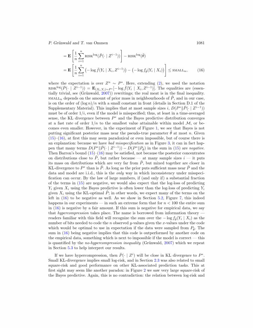
where the expectation is over Zn ∼ P ∗. Here, extending (2), we used the notationrisk

log(P (· | Zi−1)) = E(Xi,Yi)∼P∗ [− log f(Yi | Xi, Zi−1)]. The equalities are (essen-

tially trivial, see (Grunwald, 2007)) rewritings; the real meat is in the final inequality.smalln depends on the amount of prior mass in neighbourhoods of P , and in our case,is on the order of (log n)/n with a small constant in front (details in Section D.1 of theSupplementary Material). This implies that at most sample sizes i, D(P ∗‖P (· | Zi−1))must be of order 1/i, even if the model is misspecified; thus, at least in a time-averagedsense, the KL divergence between P ∗ and the Bayes predictive distribution convergesat a fast rate of order 1/n to the smallest value attainable within model M, or be-comes even smaller. However, in the experiment of Figure 1, we see that Bayes is notputting significant posterior mass near the pseudo-true parameter θ at most n. Given(15)–(16), at first this may seem paradoxical or even impossible, but of course there isan explanation: because we have bad misspecification as in Figure 3, it can in fact hap-pen that many terms D(P ∗‖P (· | Zi−1)) −D(P ∗‖Pθ) in the sum in (15) are negative.Then Barron’s bound (15)–(16) may be satisfied, not because the posterior concentrateson distributions close to P , but rather because — at many sample sizes i — it putsits mass on distributions which are very far from P , but mixed together are closer inKL-divergence to P ∗ than is P . As long as the prior puts sufficient mass near P and thedata and model are i.i.d., this is the only way in which inconsistency under misspeci-fication can occur. By the law of large numbers, if (and only if) a substantial fractionof the terms in (15) are negative, we would also expect that the log-loss of predictingYi given Xi using the Bayes predictive is often lower than the log-loss of predicting Yi

given Xi using the KL-optimal P ; in other words, we expect many of the terms on theleft in (16) to be negative as well. As we show in Section 5.2, Figure 7, this indeedhappens in our experiments — in such an extreme form that for n < 100 the entire sumin (16) is negative by a fair amount. If this sum is negative for empirical data, we saythat hypercompression takes place. The name is borrowed from information theory —readers familiar with this field will recognize the sum over the − log fθ(Yi | Xi) as thenumber of bits needed to code the n observed y-values given the x-values under the codewhich would be optimal to use in expectation if the data were sampled from Pθ. Thesum in (16) being negative implies that this code is outperformed by another code onthe empirical data, something which is next to impossible if the model is correct — thisis quantified by the no-hypercompression inequality (Grunwald, 2007) which we repeatin Section 5.3 to help interpret our results.

If we have hypercompression, then P (· | Zi) will be close in KL divergence to P ∗.Small KL-divergence implies small log-risk, and in Section 2.3 was also related to smallsquare-risk and good performance on other KL-associated prediction tasks. This atfirst sight may seem like another paradox: in Figure 2 we saw very large square-risk ofthe Bayes predictive. Again, this is no contradiction: the relation between log-risk and


square-risk (5) does not hold for arbitrary distributions, but only for members of themodel. If, as in the figure, P (· | Zi−1) is outside the model (in fact, it differs significantlyfrom any element of the model), small KL-divergence is no longer an indication thatP (· | Zi−1) will also give good results for KL-associated prediction tasks.

To see where the hypercompression in our regression example comes from, note firstthat our model is not convex: the conditional densities indexed by θ are normals withmean Xβ and fixed variance σ2 for each given X; a mixture of two such conditionalnormals can be bimodal and hence is itself not a conditional normal, hence the modelis not convex. In our setting the predictive is a mixture of infinitely many conditionalnormals. Its conditional density is a mixture of t-distributions, whose variance highlydepends on X, thus making the highly heteroskedastic predictive very different fromany of the — homoskedastic — distributions in the model. The striking difference isplotted in Figure 4. Hypercompression occurs because at X = 0, the variance of thepredictive is smaller than σ2, which substantially decreases the log-risk.

4 The Solution: How η � 1 can help, and howSafeBayes finds it

4.1 How η-generalized Bayes for η � 1 can avoid badmisspecification

We start with a re-interpretation of the η-generalized posterior: for small enough η, it isformally equivalent to a standard posterior based on a modified joint probability model2.Let f∗(x, y) be the density of the true distribution P ∗ on (X,Y ). Formally, we definethe η-reweighted distributions P (η) as joint distributions on (X,Y ) with densities f (η)

given by

f (η)(x, y | θ) = f∗(x, y) ·(f(y | x, θ)f(y | x, θ)

)η

, (17)

extended to n outcomes by independence. Now, as follows from (Van Erven et al., 2015,Example 3.7), in our setting3 there exists a critical value of η such that if we take any0 < η ≤ η, then for every θ ∈ Θ, P (η)(· | θ) is a (sub-) probability distribution, i.e. forall θ ∈ Θ, ∫ ∫

f (η)(x, y | θ)dxdy ≤ 1. (18)

If for some θ ∈ Θ, (18) is strictly smaller than 1, say 1 − ε, then the correspondingP (η)(· | θ) can be thought of as a standard probability distribution by defining it onextended outcome space (X ×Y)∪{�} and assuming that it puts mass ε on the specialoutcome � which in reality will never actually occur. We can thus think of M(η) :={P (η)(· | θ) | θ ∈ Θ} as a standard probability model. One immediately verifies that,

2In this explicit form, this insight is new and cannot be found in any of the earlier papers ongeneralized or safe Bayes, although the reweighted probabilities that we now define can be found ine.g. Van Erven et al. (2015).

3The story still goes through with some modifications if η = 0 (Grunwald and Mehta, 2016).


for every η > 0, D(P ∗‖P (η)(· | θ)) is minimized for θ, just as before — P (η)(· | θ) nowbeing equal to the ‘true’ P ∗ (!). By Bayes’ theorem, with prior π on model M(η), theposterior probability is given by:

π(θ | zn) = f (η)(xn, yn | θ) · π(θ)∫f (η)(xn, yn | θ)π(θ)ρ(dθ) =

∏ni=1 f

∗(xi, yi) ·(

f(yi|xi,θ)

f(yi|xi,θ)

)η

· π(θ)∫ ∏ni=1 f

∗(xi, yi) ·(

f(yi|xi,θ)

f(yi|xi,θ)

)η

π(θ)ρ(dθ)

=

∏ni=1 f(yi | xi, θ)

η · π(θ)∫ ∏ni=1 f(yi | xi, θ)ηπ(θ)ρ(dθ)

, (19)

which is seen to coincide with (8). Thus, as promised, for any 0 < η ≤ η, we canequivalently think of the generalized posterior as a standard posterior on a differentmodel. But for such a value of η, our use of generalized Bayesian updating is equivalentto using Bayes’ theorem in the standard way with a correctly specified probability model(because P (· | θ) = P ∗), and hence standard consistency and rate of convergence resultssuch those by Ghosal et al. (2000) kick in, and convergence of the posterior must takeplace. We can also see this in terms of Barron’s result, (15)–(16), which must also holdfor the model M(η), i.e. if we replace the standard predictive distribution P (and itsdensity f) for model M by the standard predictive for model M(η). For this reweightedmodel, we have that

0 = D(P ∗‖P (η)) ≤ D(P ∗‖P ) (20)

for any arbitrary mixture P of distributions inM(η), and therefore also for every possiblepredictive distribution P := P (· | Zi). This means that the terms in the sum in (15)are now all positive and (15)–(16) now does imply that, at most n, the Bayes predictivedistribution is close to P — so, generalized Bayes with 0 < η < η should becomecompetitive again. The ‘best’ value of η will typically be slightly smaller than, butnot equal to η: convergence of the posterior on reweighted probabilities P (η) of ordersmalln = (log n)/n corresponds to a convergence of the original probabilities P (1) atorder (logn)/(nη), so the price to pay for using a small η is that, although the posteriorwill now concentrate on the KL-optimal distribution in our model, it may take longer(by a constant factor) before this happens. The η at which the fastest convergence takesplace will thus be close to η, but in practice it may be slightly smaller, as we furtherexplain in Appendix D.2. We proceed to address the one remaining question: how todetermine η based on empirical data.

4.2 The SafeBayesian algorithm and How it finds the right η

We introduce SafeBayes via Dawid’s prequential interpretation of Bayes factor modelselection. As was first noticed by Dawid (1984) and Rissanen (1984), we can think ofBayes factor model selection as picking the model with index p that, when used forsequential prediction with a logarithmic scoring rule, minimizes the cumulative loss.To see this, note that for any distribution whatsoever, we have that, by definition ofconditional probability,

− log f(yn) = − logn∏

i=1

f(yi | yi−1) =n∑

i=1

− log f(yi | yi−1).


In particular, for the standard Bayesian marginal distribution f(· | p) = f(· | p, η = 1)as defined above, for each fixed p, we have

− log f(yn | xn, p) =

n∑i=1

− log f(yi | xn, yi−1, p) =

n∑i=1

− log f(yi | xi, zi−1, p), (21)

where the second equality holds by (9). If we assume a uniform prior on model index p,then Bayes factor model selection picks the model maximizing π(p | zn), which by Bayes’theorem coincides with the model minimizing (21), i.e. minimizing cumulative log-loss.Similarly, in ‘empirical Bayes’ approaches, one picks the value of some parameter ρthat maximizes the marginal Bayesian probability f(yn | xn, ρ) of the data. By (21),which still holds with p replaced by ρ, this is again equivalent to the ρ minimizing thecumulative log-loss. This is the prequential interpretation of Bayes factor model selectionand empirical Bayes approaches, showing that Bayesian inference can be interpreted asa sort of forward (rather than cross-) validation (Dawid, 1984; Rissanen, 1984; Hjorth,1982).

We will now see whether we can use this approach with ρ in the role of the η for theη-generalized posterior that we want to learn from the data. We continue to rewrite (21)as follows (with ρ instead of p that can either stand for a continuous-valued parameter orfor a model index but not yet for η), using the fact that the Bayes predictive distributiongiven ρ and zi−1 can be rewritten as a posterior-weighted average of fθ:

ρ := argmaxρ

f(yn | xn, ρ) = argminρ

n∑i=1

(− log f(yi | xi, z

i−1, ρ))

= argminρ

n∑i=1

(− logEθ∼Π|zi−1,ρ[f(yi | xi, θ)]

). (22)

This choice for ρ being entirely consistent with the (empirical) Bayesian approach, ourfirst idea is to choose η in the same way: we simply pick the η achieving (22), withρ substituted by η. However, this will tend to pick η close to 1 and does not improvepredictions under misspecification — this is illustrated experimentally in Section 5.4;see also (Grunwald and Van Ommen, 2014, Figure 13). But it turns out that a slightmodification of (22) does the trick: we simply interchange the order of logarithm andexpectation in (22) and pick the η minimizing

n∑i=1

Eθ∼Π|zi−1,η [− log f(yi | xi, θ)] . (23)

In words, we pick the η minimizing the posterior-expected posterior-Randomized log-loss, i.e. the log-loss we expect to obtain, according to the η-generalized posterior, ifwe actually sample from this posterior. This modified loss function has also been calledGibbs error (Cuong et al., 2013); we simply call it the η-R-log-loss from now on.

We now give a heuristic explanation of why (22) (with ρ = η) fails while (23) works;a much more detailed explanation is in the supplementary material. The problem with(22) is that it tends to be small for η at which hypercompression takes place. By (15),at η at which bad misspecification and hence hypercompression takes place — someof the terms inside the expectation in (15) are negative — we also expect some of the


terms in (16) to be negative. In Figure 7 we will see that in our experiments, thisindeed happens. (22) can thus become very small — smaller than the cumulative losswe would get if we would persistently predict with the optimal θ — for η = 1 or close to1. These are the η for which we have already established that Bayes fails. In contrast,the Gibbs error (23) is small in expectation only if a substantial part of the posteriormass is assigned to θ close to θ in the sense that D(P ∗‖Pθ)−D(P ∗‖Pθ) is small. Thisstricter requirement clearly cannot favour η at which hypercompression takes place, anddirectly targets η∗ at which the posterior mass concentrates around the optimal θ — soSafeBayes can be expected to perform well as long as such η∗ exists. Barron’s theoremin combination with (20) implies (ignoring some subtleties explained in the appendix)that for η∗ < η, for all large enough n (depending on η∗), the η∗-generalized posteriorindeed concentrates around θ, so that SafeBayes will tend to find such an η∗.

In practice, it is computationally infeasible to try all values of η and we simply haveto try out a grid of values, where, as shown by Grunwald (2012), it is sufficient to let gridpoints decrease exponentially fast. For convenience we give a detailed description of thealgorithm below, copied from Grunwald (2012). In the present paper, we will invariablyapply the algorithm with zi = (xi, yi) as before, and θ(zi) set to the (conditional)log-loss as defined before.

Algorithm 1: The (R-)SafeBayesian algorithm

Input: data z1, . . . , zn, model M = {f(· | θ) | θ ∈ Θ}, prior Π on Θ, step-sizeκstep, max. exponent κmax, loss function θ(z)

Output: Learning rate ηSn := { 1, 2−κstep , 2−2κstep , 2−3κstep , . . . , 2−κmax };for all η ∈ Sn do

sη := 0;for i = 1 . . . n do

Determine generalized posterior Π(· | zi−1, η) of Bayes with learning rateη.Calculate “posterior-expected posterior-randomized loss” of predictingactual next outcome:

r := Π|zi−1,η(zi) = Eθ∼Π|zi−1,η [θ(zi)] (24)

sη := sη + r;

end

endChoose η := argminη∈Sn

{ sη } (if min achieved for several η ∈ Sn, pick largest);

Variation Wemay also consider the η which, instead of the η-R-log-loss ((23) and (24)),minimizes the η-in-model-log-loss (or just η-I-log-loss), defined as

n∑i=1

[− log f(yi | xi,Eθ∼Π|zi−1,η[θ])

]. (25)


We call the version of SafeBayes which minimizes the alternative objective function(25) in-model SafeBayes, abbreviated to I-log-SafeBayes, and from now on use R-log-SafeBayes for the original version based on the R-log-loss. Like (23), (25) cannot ex-ploit hypercompression: it measures prediction error using the log score of a distributionwithin M(η), whereas hypercompression only occurs if a distribution outside M(η) isused; otherwise though, it is quite different from (23), and further illuminating motiva-tion is provided in Section C.1 in the supplementary material. The theoretical results ofGrunwald (2012) do not give any clue as to whether to prefer the I- or the R-versions,and a secondary goal of the experiments in this paper is thus to see whether one of themis always preferable over the other (we find that the answer is no). Explicit formulasinstantiating both versions of SafeBayes to the linear model are given in Section C.1 inthe supplement; Section C.3 recalls some theoretical results on SafeBayes’ convergencebehaviour.

5 Main experiment

In this section we provide our main experimental results, based on linear models Mp

as defined in Section 2.2. Figures 5 and 6 depict, and Section 5.2 discusses the resultsof model selection and averaging experiments, which choose or average between themodels 0, . . . , pmax, where we consider first an incorrectly and then a correctly specifiedmodel, both with pmax = 50; Figures G.1 and G.2 in the supplement do the same forpmax = 100. Section 5.4 contains and interprets additional experiments on Bayesianridge regression, with a fixed p; a multitude of additional experiments checking whetherour results hold under model, prior and ground truth variations is provided in [GvO].The final Section 6 summarizes the relevant findings of both the experiments belowand these additional experiments. But first we need to explain the priors π and thesampling (‘true’) distributions P ∗ with which we experiment: as to the priors, in ourmodel selection/averaging experiments, we use a fat-tailed prior on the models given by

π(p) ∝ 1

(p+ 2)(log(p+ 2))2.

This prior was chosen because it remains well-defined for an infinite collection of models,even though we only use finitely many in our experiments. As a sanity check we repeatedsome of our experiments with a uniform prior on 0, . . . , pmax instead; the results wereindistinguishable. Each model Mp has parameters β, σ2, on which we put the standardconjugate priors as described in Section 2.5. We set the mean of the prior on β toβ0 = 0, and its covariance matrix to σ2Σ0 setting Σ0 to the identity matrix Σ0 = Ip+1;the hyperparameters on the variance are set to a0 = 1 and b0 = 40; in Appendix C.2we explain the reasons for this choice and alternatives we experimented with as well.

Concerning ground truth P ∗, our experiments fall into two categories: correct-modeland wrong-model experiments. In the correct-model experiments,X1, X2, . . . are sampledi.i.d., with, for each individual Xi = (Xi1, . . . , Xipmax), Xi1 . . . , Xipmax i.i.d. ∼ N(0, 1).Given each Xi, Yi is generated as

Yi = .1 · (Xi1 + . . .+Xi4) + εi, (26)


where the εi are i.i.d. ∼ N(0, σ∗2) with variance σ∗2 = 1/40. In contrast, in the wrong-model experiments, at each time point i, a fair coin is tossed independently of everythingelse. If the coin lands heads, then the point is ‘easy’, and (Xi, Yi) := (0, 0). If the coinlands tails, then Xi is generated as for the correct model, and Yi is generated as (26), butnow the noise random variables have variance σ2

0 = 2σ∗2 = 1/20. Thus, Zi = (Xi, Yi)is generated as in the true model case but with a larger variance; this larger variancehas been chosen so that the marginal variance of each Yi is the same value σ∗2 in bothexperiments.

From the results in Section 2.3 we immediately see that, for both experiments,the optimal model is Mp for p = 4, and the optimal distribution in M and Mp is

parameterized by θ = (p, β, σ2) with p = 4, β = (β0, . . . β4) = (0, .1, .1, .1, .1), σ2 = 1/40(in the correct model experiment, σ2 = σ∗2; in the wrong model experiment, sinceσ2 must be reliable, it must be equal to the square-risk obtained with (p, β), whichis (1/2) · (1/20) = 1/40). f(x) := xβ is then equal to the true regression functionEP∗ [Y | X].

Variations We have already seen a variation of these two experiments depicted inFigures 1 and 2. In the correct-model version of that experiment, P ∗ is defined as follows:set Xj = Pj(S), where Pj is the Legendre polynomial of degree j and S is uniformlydistributed on [−1, 1], and set Y = 0 + ε, where ε ∼ N(0, σ∗2), with σ∗2 = 1/40;(X1, Y1), . . . are then sampled as i.i.d. copies of (X,Y ). Note that the true regressionfunction is 0 here. In [GvO] we briefly consider this and several other variations of theseground truths.

5.1 The statistics we report

Figure 5 reports the results of the wrong-model experiment, and Figure 6 of the correct-model experiment, both with pmax = 50. For both experiments we measure three aspectsof the performance of Bayes and SafeBayes, each summarized in a separate graph. First,we show the behaviour of several prediction methods based on SafeBayes relative tosquare-risk; second, we check a form of model identification consistency; third, we mea-sure whether the methods provide a good assessment of their own predictive capabilitiesin terms of square-loss, i.e. whether they are reliable and not ‘overconfident’. Below weexplain these three performance measures in detail. We also provide a fourth graph ineach case indicating what η’s are typically selected by the two versions of SafeBayes.

Square-risk For a given distribution W on (p, β, σ2), the regression function based onW , a function mapping covariate X to R, abbreviated to EW [Y | X], is defined as

EW [Y | X] := E(p,β,σ)∼W EY∼Pp,β,σ|X [Y ] = E(p,β,σ)∼W

⎡⎣ p∑j=0

βjXj

⎤⎦ . (27)

If we take W to be the η-generalized posterior, then (27) is also simply called the η-posterior regression function. The square-risk relative to P ∗ based on predicting by Wis then defined as an extension of (4) as


Figure 5: Four graphs showing respectively the square-risk, MAP model order, over-confidence (lack of reliability), and selected η at each sample size, each averaged over30 runs, for the wrong-model experiment with pmax = 50, for the methods indicated inSection 5.1. For the selected-η graph, the pale lines are one standard deviation apartfrom the average; all lines in this graph were computed over η indices (so that the linesdepict the geometric mean over the values of η themselves).


Figure 6: Same graphs as in Figure 5 for the correct-model experiment with pmax = 50.


risksq(W ) := E(X,Y )∼P∗(Y −EW [Y | X])2. (28)

In the experiments below we measure the square-risk relative to P ∗ at sample size i− 1achieved by, respectively, (1), the η-generalized posterior, and (2), the η-generalizedposterior conditioned on the MAP (maximum a posteriori) model, i.e.

EZi−1∼P∗ [risksq(W )], with W = Π | Zi−1, η ; W = Π | Zi−1, η, pmap(Zi−1,η) (29)

respectively, where the MAP model pmap(Zi−1,η) is defined as the p achievingmaxp∈0,...,pmax π(p | Zi−1, η), with π(p | Zi−1, η) defined as in (11). We do this for threevalues of η: (a) η = 1, corresponding to the standard Bayesian posterior, (b) η := η(Zi−1)set by the R-log SafeBayesian algorithm run on the past data Zi−1, and (c) η set bythe I-log SafeBayesian algorithm. In the figures of Section 5.2, 1(a) is abbreviated toBayes, 1(b) is R-log-SafeBayes, 1(c) is I-log-SafeBayes, 2(a) is Bayes MAP, 2(b) isR-log-SafeBayes MAP, and 2(c) is I-log-SafeBayes MAP.

Concerning the two square-risks that we record: The first choice is the most natural,corresponding to the prediction (regression function) according to the ‘standard’ η-generalized posterior. The second corresponds to the situation where one first selects asingle submodel pmap and then bases all predictions on that model; it has been includedbecause such methods are often adopted in practice.

In Figure 5 and subsequent figures below, we depict these quantities by sequentiallysampling data Z1, Z2, . . . , Zmax i.i.d. from a P ∗ as defined above, where max is somelarge number. At each i, after the first i−1 points Zi−1 have been sampled, we computethe two square-risks given above. We repeat the whole procedure a number of times(called ‘runs’); the graphs show the average risks over these runs.

MAP-model identification / Occam’s razor When the goal of inference is model iden-tification, ‘consistency’ of a method is often defined as its ability to identify the smallestmodel Mp containing the ‘pseudo-truth’ (β, σ2). To see whether standard Bayes and/orSafeBayes are consistent in this sense, we check whether the MAP model pmap(Zi−1,η)

is equal to p.

Reliability vs. overconfidence Does Bayes learn how good it is in terms of squarederror? To answer this question, we define, for a predictive distribution W as in (28)

above, U[W ]i (a function of Xi, Yi and (through W ) of Zi−1), as

U[W ]i = (Yi −EW [Yi | Xi])

2.

This is the error we make if we predict Yi using the regression function based on pre-diction method W . In the graphs in the next sections we plot the self-confidence ratio

EXi,Yi∼P∗ [U[W ]i ]/EXi∼P∗ EYi∼W |Xi

[U[W ]i ] as a function of i for the three prediction

methods / choices of W defined above. We may think of this as the ratio betweenthe actual expected prediction error (measured in square-loss) one gets by using apredictor who based predictions on W and the marginal (averaged over X) subjec-tively expected prediction error by this predictor. We previously, in Section 2.3, showed


that the KL-optimal (p, β, σ2) is reliable: this means that, if we would take W thepoint mass on (p, β, σ2) and thus, irrespective of past data Zi−1, would predict by

E(p,β,σ2)[Yi | Xi] =∑p

j=0 βjXij , then the ratio would be 1. For the W learned fromdata considered above, a value larger than 1 indicates that W does not implement a‘reliable’ method in the sense of Section 2.3, but, rather, is overconfident: it predicts itspredictions to be better than they actually are, in terms of square-risk.

5.2 Main model selection/averaging experiment

We run the SafeBayesian algorithm of Section 4.2 with zi = (xi, yi) and θ(zi) =− log fθ(yi | xi) is the (conditional) log-loss as described in that section. As to theparameters of the algorithm, in all experiments we set the step-size κstep = 1/3 andκmax := 8, i.e. we tried the following values of η: 1, 2−1/3, 2−2/3, . . . , 2−8. The resultsof, respectively, the wrong-model and correct-model experiment as described above,with pmax = 50, are given in Figures 5 and 6; results for pmax = 100 can be found inFigures G.1 and G.2 in the supplement.

Conclusion 1: Bayes performs well in model-correct, and dismally in model-incorrectexperiment The four figures show that standard Bayes behaves excellently in termsof all quality measures (square-risk, MAP model identification and reliability) when themodel is correct, and dismally if the model is incorrect.

Conclusion 2: If (and only if) model incorrect, then the higher pmax, the worse Bayesgets We see from Figures 6 and G.2 that standard Bayes behaves excellently in termsof all quality measures (square-risk, MAP model identification and reliability) when themodel is correct, both if pmax = 50 and if pmax = 100, the behaviour at pmax = 100 beingessentially indistinguishable from the case with pmax = 50. These and other (unreported)experiments strongly suggests that, when the data are sampled from a low-dimensionalmodel, then, when the model is correct, standard Bayes is unaffected (does not getconfused) by adding additional high-dimensional models to the model space. Indeed,the same is suggested by various existing Bayesian consistency theorems, such as thoseby Doob (1949); Ghosal et al. (2000); Zhang (2006a). At the same time, from Figures 5and G.1 we infer that standard Bayes behaves very badly in all three quality measuresin our (admittedly very ‘evilly chosen’) model-wrong experiment. Eventually, at verylarge sample sizes, Bayes recovers, but the main point here to notice is that the nat which a given level of recovery (measured in, say, square-loss) takes place is muchhigher for the case pmax = 100 (Figure G.1) than for the case pmax = 50 (Figure 5). Thisstrongly suggests that, when the model is incorrect but the best approximation lies ina low-dimensional submodel, then standard Bayes gets confused by adding additionalhigh-dimensional models to the model space — recovery takes place at a sample sizethat increases with pmax. Indeed, the graphs suggest that in the case that pmax = ∞(with which we cannot experiment), Bayes will be inconsistent in the sense that therisk of the posterior predictive will never ever reach the risk attainable with the bestsubmodel. Grunwald and Langford (2007) showed that this can indeed happen with a


simple, but much more unnatural classification model; the present result indicates (butdoes not mathematically prove) that it can happen with our standard model as well;see also the discussion in Section G.2.

Conclusion 3: R-log-SafeBayes and I-log-SafeBayes generally perform well Com-paring the four graphs for R-log-SafeBayes and I-log-SafeBayes, we see that they behavequite well for both the model-correct and the model-wrong experiments, being slightlyworse than, though still competitive to, standard Bayes when the model is correct andincomparably better when the model is wrong. Indeed, in the wrong-model experiments,about half of the data points are identical and therefore do not provide very much infor-mation, so one would expect that if a ‘good’ method achieves a given level of square-riskat sample size n in the correct-model experiment, it achieves the same level at about 2nin the incorrect-model experiment, and this is indeed what happens. Also, we see fromcomparing Figures G.1 and G.2 on the one hand to Figures 5 and 6 on the other thatadding additional high-dimensional models to the model space hardly affects the re-sults — like standard Bayes when the model is correct, SafeBayes does not get confusedby living in a larger model space.

Secondary conclusions We see that both types of SafeBayes converge quickly to theright (pseudo-true) model order, which is pleasing since they were not specifically de-signed to achieve this. Whether this is an artefact of our setting or holds more generallywould, of course, require further experimentation. We note that at small sample sizes,when both types of SafeBayes still tend to select an overly simple model, I-log-SafeBayeshas significantly more variability in the model chosen-on-average; it is not clear thoughwhether this is ‘good’ or ‘bad’. We also note that the η’s chosen by both versions are verysimilar for all but the smallest sample sizes, and are consistently smaller than 1. Wheninstead of the full η-generalized posteriors, the η-generalized posterior conditioned onthe MAP pmap is used, the behaviour of all method consistently deteriorates a little,but never by much.

5.3 Experimental demonstration of hypercompression for standardBayes

Figure 7 and Figure 8 show the predictive capabilities of standard Bayes in the wrongmodel example in terms of cumulative and instantaneous log-loss on a simulated sample.The graphs clearly demonstrate hypercompression: the Bayes predictive cumulativelyperforms better than the best single model / the best distribution in the model space,until at about n ≈ 100 there is a phase transition. At individual points, we see that itsometimes performs a little worse, and sometimes (namely at the ‘easy’ (0, 0) points)much better than the best distribution. We also see that, as anticipated above, forη = 1 randomized and in-model Bayesian prediction (used respectively by R- and I-log-SafeBayes to choose η) do not show hypercompression and in fact perform terribly onthe log-loss until the phase transition at n = 100, when they become almost as good asprediction with the Bayesian mixture.


Figure 7: Cumulative standard, R-, and I-log-loss as defined in (23) and (25) respec-tively of standard Bayesian prediction (η = 1) on a single run for the model-averagingexperiment of Figure 5. We clearly see that standard Bayes achieves hypercompres-sion, being better than the best single model. And, as predicted by theory, randomizedBayes is never better than standard Bayes, whose curve has negative slope because thedensities of outcomes are > 1 on average.

Figure 8: Instantaneous standard, R- and I-log-loss of standard Bayesian prediction forthe run depicted in Figure 7.

The no-hypercompression inequality In fact, Figure 7 shows a phenomenon that isvirtually impossible if the Bayesian’s model and prior are ‘correct’ in the sense that dataZn would behave like a typical sample from them: it easily follows from Markov’s in-equality (for details see Grunwald, 2007, Chapter 3) that, letting Π denote the Bayesian’sjoint distribution on Θ×Zn, for each K ≥ 0,

Π

{(θ, Zn) :

n∑i=1

(− log f(Yi | Xi, Z

i−1))≤

n∑i=1

(− log fθ(Yi | Xi, Z

i−1))−K

}≤ e−K ,

i.e. the probability that the Bayes predictive f cumulatively outperforms fθ, with θdrawn from the prior, by K log-loss units is exponentially small in K. Figure 7 thusshows that at sample size n ≈ 90, an a priori formulated event has happened of proba-bility less than e−30, clearly indicating that something about our model or prior is quitewrong.


Since the difference in cumulative log-loss between f and fθ can be interpreted asthe amount of bits saved when coding data from fθ with a lossless code that wouldbe optimal in expectation under f rather than fθ, this result has been called the no-hypercompression inequality by Grunwald (2007). The figure shows that for our data,we have substantial hypercompression.

5.4 Second experiment: Bayesian ridge regression

We repeat the model-wrong and model-correct experiments of Figures 5 and 6, with justone difference: all posteriors are conditioned on p := pmax = 50. Thus, we effectivelyconsider just a fixed, high-dimensional model, whereas the best approximation θ =(50, β, σ2) viewed as an element of Mp is ‘sparse’ in that it has only β1, . . . , β4 not equalto 0. We note that the MAP model index graphs of Figures 5 and 6 are meaningless inthis context (they would be equal to the constant 50) so they are left out of the newFigures 9 and 10. Results for Cesaro-averaged posteriors are shown instead; we refer toSection C.3 in the supplementary material for their definition and relevance.

Connection to Bayesian (b)ridge regression From (13) we see that the posteriormean parameter βi,η is equal to the posterior MAP parameter and depends on η butnot on σ2, since σ2 enters the prior in the same way as the likelihood. Therefore, thesquare-loss obtained when using the generalized posterior for prediction is always givenby (yi − xiβi−1,η)

2 irrespective of whether we use the posterior mean, or MAP, or thevalue of σ2. Interestingly, if we fix some λ and perform standard (nongeneralized) Bayeswith a modified prior, proportional to the original prior raised to the power λ := η−1,then the prior, conditioned on σ2, becomes normal N(β0, σ

2Σ′0) where Σ′

0 = ηΣ0 andthe standard posterior given zi is then (by (13)) Gaussian with mean(

(Σ′0)

−1+X�

nX)−1

·((Σ′

0)−1

β0 +X�ny

n)= βi,η. (30)

Thus we see that in this special case, the (square-risk of the) η-generalized Bayes pos-terior mean coincides with the (square-risk of the) standard Bayes posterior mean withprior N(β0, σ

2ηΣ0) given σ2, for arbitrary prior on σ2. We first note that if Σ0 is theidentity matrix, then this implies that, for fixed η, the η-generalized Bayes posteriormean coincides with the ridge regression estimate with penalty parameter λ := η−1. Forgeneral Σ0, it implies that the posterior on β coincides with the posterior one gets withBayesian ridge regression, as defined, by4, e.g., Park and Casella (2008), conditionedon setting the λ-parameter in Bayesian ridge regression equal to η−1. Now, the gen-eral Bayesian ridge regression method has λ as a free parameter, determined either byempirical Bayes or equipped with a prior. It is thus of interest to see what happens if,rather than using SafeBayes, we determine η (equivalently, λ) in this way. In additionto the graphs discussed earlier in Section 5.1, we thus also show the results for η set byempirical Bayes (in separate experiments not shown here we confirmed that putting a

4To be precise, they call this method Bayesian ‘bridge’ regression with q = 2; the choice of q = 1 intheir formula gives their celebrated ‘Bayesian Lasso’.


Figure 9: Bayesian ridge regression: Model-wrong experiment conditioned on p :=pmax = 50. The graphs (square-risk, self-confidence ratio and chosen η as functionof sample size) are as in Figures 5 and 6, except for the third graph there (MAP modelorder), which has no meaning here. The meaning of the curves is given in Section 5.1except for empirical Bayes, explained in Section 5.4.


Figure 10: Bayesian ridge regression: Same graphs as in Figure 9, but for the model-correct experiment conditioned on p := pmax = 50.

prior on η and using the full posterior on η gives essentially the same results). Whereasthe empirical-Bayesian ridge regression is known to be a very competitive method inmany practical settings (indeed in our model-correct experiment, Figure 10, it performsbest in all respects), we see in Figure 9 (the green line) that, just like other versions of


Bayes, it breaks down under our type of misspecification. We hasten to add that thecorrespondence between the η-generalized posterior means and the standard posteriormeans with prior raised to power 1/η only holds for the βi,η parameters. It does not holdfor the σ2

i,η parameters, and thus, for fixed η, the self-confidence ratio of both methodsmay be quite different.

Conclusions for model-wrong experiment For most curves, the overall picture ofFigure 9 is comparable to the corresponding model averaging experiment, Figure 5:when the model is wrong, standard Bayes shows dismal performance in terms of riskand reliability up to a certain sample size and then very slowly recovers, whereas bothversions of SafeBayes perform quite well even for small sample sizes. We do not showvariations of the graph for p = pmax = 100 (i.e. the analogue of Figure G.1), since itrelates to Figure 9 in exactly the same way as Figure G.1 relates to Figure 5: withp = 100, bad square-risk and reliability behaviour of Bayes goes on for much longer(recovery takes place at much larger sample size) and remains equally good as forp = 50 with the two versions of SafeBayes.

We also see that, as we already indicated in the introduction, choosing the learningrate by empirical Bayes (thus implementing one version of Bayesian bridge regression)behaves terribly. This complies with our general theme that, to ‘save Bayes’ in generalmisspecification problems, the parameter η cannot be chosen in a standard Bayesianmanner.

Conclusions for model-correct experiment The model-correct experiment for ridgeregression (Figure 10) offers a surprise: we had expected Bayes to perform best, and weresurprised to find that the SafeBayeses obtained smaller risk. Some followup experiments(not shown here), with different true regression functions and different priors, shedmore light on the situation. Consider the setting in which the coefficients of the truefunction are drawn randomly according to the prior. In this setting standard Bayesperforms at least as good in expectation as any other method including SafeBayes (theBayesian posterior now represents exactly what an experimenter might ideally know).SafeBayes (still in this setting) usually chooses η = 1/2 or 1/4, and the difference inrisks compared to Bayes is small. On the other hand, if the true coefficients are drawnfrom a distribution with substantially smaller variance than a priori expected by theprior (a factor 1000 in the ‘correct’-model experiment of Figure 10), then SafeBayesperforms much better than Bayes. Here Bayes can no longer necessarily be expectedto have the best performance (the model is correct, but the prior is “wrong”), andit is possible that a slightly reduced learning rate gives (significantly) better results.It seems that this situation, where the variance of the true function is much smallerthan its prior expectation, is not exceptional: for example, Raftery et al. (1997) suggestchoosing the variance of the prior in such a way that a large region of parameter valuesreceives substantial prior mass. Following that suggestion in our experiments alreadygives a variance that is large enough compared to the true coefficients that SafeBayesperforms better than Bayes even if the model is correct.


A joint observation for the model-wrong and model-correct experiments Finallywe observe an interesting difference between the two SafeBayes versions here: I-log-SafeBayes seems better for risk, giving a smooth decreasing curve in both experiments.R-log-SafeBayes inherits a trace of standard Bayes’ bad behaviour in both experiments,with a nonmonotonicity in the learning curve. On the other hand, in terms of reliability,R-log-SafeBayes is consistently better than I-log-SafeBayes (but note that the latter isunderconfident, which is arguably preferable over being overconfident, as Bayes is). Allin all, there is no clear winner between the two methods.

6 Executive summary: Main conclusions fromexperiments

Here we summarize the most important conclusions from our main experiments de-scribed above, as well as from the many variations of these main experiments that weperformed to check the robustness of our conclusions in the technical report [GvO].

Standard Bayes In almost all our experiments, standard Bayesian inference fails in itsKL-associated prediction tasks (squared error risk, reliability) when the model is wrong.Adopting a different prior (such as the g-prior) does not help, with two exceptions inmodel averaging: (a) if using a prior that follows the suggestions of Raftery et al. (1997),then Bayes works quite well with 50% ‘easy’ points, but starts to fail dramatically again(in contrast to SafeBayes) once the percentage of easy points is increased a bit further;(b) when it is run with a fixed variance that is significantly larger than the ‘best’(pseudo-true) variance σ2. Moreover, in the ridge regression experiments, as reportedabove, we find that standard Bayes can even perform much worse than SafeBayes whenthe model is correct — so all in all we tentatively conclude that SafeBayes is safer touse for linear regression.

SafeBayes The two SafeBayes methods discussed here behave reasonably well in allour experiments, and there is no clear winner among them. I-log-SafeBayes usuallybehaves excellently in terms of square-risk but is underconfident about its own per-formance (which is perhaps acceptable, overconfidence being a lot more dangerous).R-log-SafeBayes is usually good in terms of square-risk though not as good as I-log-SafeBayes, yet it is highly reliable. In [GvO] we additionally experiment with versionsof SafeBayes for fixed-variance models, or, equivalently, for generalized posteriors of thegeneric form (7) with a squared loss function (the I-version (C.1) is discussed in the sup-plementary material, Section C.1). We find that (and explain why) for such cases, theR-method is not competitive with the I-method; the I-method works well for squarederror prediction but, since it cannot learn σ2 from the data, cannot be used to assessreliability (further explained in Section D.2).

Learning η in Bayes- or likelihood way/Bayesian ridge regression fails Despite itsintuitive appeal, fitting η to the data by e.g. empirical Bayes fails in the model-wrong


ridge experiment with a prior on σ2, where, as explained above, it amounts to Bayesianridge regression (Figure 9). In [GvO] we also consider Bayesian ridge regression with afixed variance, i.e. a degenerate prior that concentrates on a single σ2. As we explainthere, in this setting empirical Bayes learning of η reduces to empirical Bayes learningof the variance (since η−1 now plays just the same role as σ2/2), and again it leads tovery bad results in our model-wrong experiment. This latter empirical Bayes methodfor learning η is also related to one of the methods advocated by Bissiri et al. (2016),to which we return in Section F.

Robustness of experiments It does not matter whether the Xi1, Xi2, . . . are indepen-dent Gaussian, uniform or represent polynomial basis functions: all phenomena reportedhere persist for all choices. If the ‘easy’ points are not precisely (0, 0), but have them-selves a small variance in both dimensions, then all phenomena reported here persist,but on a smaller scale.

Centring We repeated several of our experiments with centred data, i.e. preprocesseddata so that the empirical average of the Yi is exactly 0 (Raftery et al., 1997; Hastieet al., 2001). In none of our experiments did this affect any results. We also looked atthe case where the true regression function has an intercept far from 0, and data arenot centred. This hardly affected the SafeBayes methods.

Other methods We also repeated the wrong-model experiment for several other meth-ods of model selection: AIC (Akaike’s Information Criterion), BIC (Bayesian Informa-tion Criterion), and various forms of cross-validation. Briefly, we found that all thesehave severe problems with our data as well. In these experiments, the mentioned meth-ods were used to identify a model index p and η played no role. We also did an ex-periment where we used leave-one-out cross-validation to learn η itself. When we triedit with log-loss (as a likelihoodist or information-theorist might be tempted to do),it behaved terribly. However, with the squared error loss it worked fine in the sensethat it achieved small squared error risk, which is not too surprising given its closesimilarity to the I-version of SafeBayes with a fixed variance (see Section C.1 in theSupplementary Material). Thus, we tentatively conclude (not surprisingly perhaps) thatcross-validation based on the squared error loss works well if one is interested in thesquared error risk; but it cannot be used for the other KL-associated prediction task,i.e. assessing reliability (Section D.2).

Real-world data Finally, we note that (De Heide, 2016b) is a preliminary report onsome regression experiments with trigonometric basis functions, performed using the R-package SafeBayes (De Heide, 2016a). De Heide found that the phenomenon describedin this paper also takes place for some real world data sets, namely daily maximumtemperatures at the Seattle airport and air pollution data from the Openair Projectat King’s College, London (Carslaw and Ropkins, 2012). These data sets do appearheteroskedastic, and she finds that standard Bayes overfits and is substantially out-performed by SafeBayes, just as in Figure 2. Similarly, Quadrianto and Ghahramani


(2015) and Devaine et al. (2013) report good performance of SafeBayes-like methods inpractice.

Supplementary Material

Supplementary material of “Inconsistency of Bayesian Inference for Misspecified LinearModels, and a Proposal for Repairing It” (DOI: 10.1214/17-BA1085SUPP; .pdf). Inthis paper, we described a problem for Bayesian inference under misspecification, andproposed the SafeBayes algorithm for solving it. The main appendix, Appendix B, placesSafeBayes in proper context by giving a six point overview of what can go wrong inBayesian inference from a frequentist point of view, and what can be done about it,both in the well- and in the misspecified case. Specifically we clarify the one otherproblem with Bayes under misspecification — interest in non-KL-associated tasks —and its relation to Gibbs posteriors. The remainder of the supplement is devoted todiscussing these six points in great detail, explicitly stating several Open Problems,related work, and ideas for a general Bayesian misspecification theory as we go along.We also provide further details on SafeBayes (Appendix C), additional experiments(Appendix G) and refine and explain in more detail the notion of bad misspecificationand hypercompression (Appendix D).

ReferencesAudibert, J. Y. (2004). “PAC-Bayesian statistical learning theory.” Ph.D. thesis, Uni-versite Paris VI. 1077

Barron, A. R. (1998). “Information-Theoretic Characterization of Bayes Perfor-mance and the Choice of Priors in Parametric and Nonparametric Problems.”In Bernardo, J. M., Berger, J. O., Dawid, A. P., and Smith, A. F. M. (eds.), BayesianStatistics, volume 6, 27–52. Oxford: Oxford University Press. 1071, 1080

Barron, A. R. and Cover, T. M. (1991). “Minimum Complexity Density Estimation.”IEEE Transactions on Information Theory , 37(4): 1034–1054. MR1111806. 1071

Bissiri, P. G., Holmes, C., andWalker, S. G. (2016). “A General Framework for UpdatingBelief Distributions.” Journal of the Royal Statistical Society, Series B (StatisticalMethodology), 78(5): 1103–1130 . 1072, 1077, 1099

Carslaw, D. C. and Ropkins, K. (2012). “Openair – an R package for air quality dataanalysis.” Environmental Modelling and Software, 27(18): 52–61. 1099

Catoni, O. (2007). PAC-Bayesian Supervised Classification. Lecture Notes-MonographSeries. IMS. MR2483528. 1077

Cuong, N. V., Lee, W. S., Ye, N., Chai, K. M. A., and Chieu, H. L. (2013). “ActiveLearning for Probabilistic Hypotheses Using the Maximum Gibbs Error Criterion.”In Advances in Neural Information Processing Systems 26 . 1084

Dawid, A. P. (1984). “Present Position and Potential Developments: Some Personal

http://dx.doi.org/10.1214/17-BA1085SUPP

http://www.ams.org/mathscinet-getitem?mr=1111806



Views, Statistical Theory, The Prequential Approach.” Journal of the Royal StatisticalSociety, Series A, 147(2): 278–292. MR0763811. 1083, 1084

De Blasi, P. and Walker, S. G. (2013). “Bayesian asymptotics with misspecified models.”Statistica Sinica, 23: 169–187. 1070, 1073

Devaine, M., Gaillard, P., Goude, Y., and Stoltz, G. (2013). “Forecasting electricityconsumption by aggregating specialized experts; a review of the sequential aggregationof specialized experts, with an application to Slovakian and French country-wide one-day-ahead (half-)hourly predictions.”Machine Learning , 90(2): 231–260. MR3015743.1100

Diaconis, P. and Freedman, D. (1986). “On the Consistency of Bayes Estimates.” TheAnnals of Statistics, 14(1): 1–26. MR0829555. 1073

Doob, J. L. (1949). “Application of the theory of martingales.” In Le Calcul deProbabilites et ses Applications. Colloques Internationaux du Centre National de laRecherche Scientifique, 23–27. Paris. 1091

Van Erven, T., Grunwald, P., Mehta, N., Reid, M., and Williamson, R. (2015). “FastRates in Statistical and Online Learning.” Journal of Machine Learning Research.Special issue in Memory of Alexey Chervonenkis. MR3417799. 1082

Ghosal, S., Ghosh, J., and Van der Vaart, A. (2000). “Convergence rates of posteriordistributions.” Annals of Statistics, 28(2): 500–531. MR1790007. 1070, 1083, 1091

Grunwald, P. D. (1998). “The Minimum Description Length Principle and Reasoningunder Uncertainty.” Ph.D. thesis, University of Amsterdam, The Netherlands. Avail-able as ILLC Dissertation Series 1998-03; see www.grunwald.nl. 1076

Grunwald, P. D. (1999). “Viewing all Models as “Probabilistic”.” In Proceedings of theTwelfth ACM Conference on Computational Learning Theory (COLT’ 99), 171–182.1076

Grunwald, P. D. (2007). The Minimum Description Length Principle. Cambridge, MA:MIT Press. 1081, 1093, 1094

Grunwald, P. D. (2011). “Safe Learning: Bridging the gap between Bayes, MDL andstatistical learning theory via empirical convexity.” In Proceedings of the Twenty-Fourth Conference on Learning Theory (COLT’ 11). 1071, 1077

Grunwald, P. D. (2012). “The Safe Bayesian: Learning the learning rate via the mix-ability gap.” In Proceedings 23rd International Conference on Algorithmic LearningTheory (ALT ’12). Springer. 1071, 1077, 1085, 1086

Grunwald, P. D. (2017). “Safe Probability.” Journal of Statistical Planning and Infer-ence. doi: http://dx.doi.org/10.1016/j.jspi.2017.09.014. To appear. 1074

Grunwald, P. D. and Langford, J. (2004). “Suboptimality of MDL and Bayes in clas-sification under misspecification.” In Proceedings of the Seventeenth Conference onLearning Theory (COLT’ 04). New York: Springer-Verlag. 1073

Grunwald, P. D. and Langford, J. (2007). “Suboptimal behavior of Bayes and






www.grunwald.nl

http://dx.doi.org/10.1016/j.jspi.2017.09.014


MDL in classification under misspecification.” Machine Learning , 66(2–3): 119–149.doi: http://dx.doi.org/10.1007/s10994-007-0716-7. 1073, 1091

Grunwald, P. D. and Mehta, N. A. (2016). “Fast Rates with Unbounded Losses.” arXivpreprint arXiv:1605.00252. 1074, 1082

Grunwald, P. D. and Van Ommen, T. (2014). “Inconsistency of Bayesian Inferencefor Misspecified Linear Models, and a Proposal for Repairing It.” arXiv preprintarXiv:1412.3730. 1073, 1084

Grunwald, P. D. and Van Ommen, T. (2017). “Supplementary material of “Inconsistencyof Bayesian Inference for Misspecified Linear Models, and a Proposal for RepairingIt”.” Bayesian Analysis. doi: http://dx.doi.org/10.1214/17-BA1085SUPP. 1070

Hastie, T., Tibshirani, R., and Friedman, J. (2001). The Elements of Statistical Learn-ing: Data Mining, Inference and Prediction. Springer Verlag. 1099

De Heide, R. (2016a). “R-Package SafeBayes.” Freely available at CRAN Repository.1072, 1099

De Heide, R. (2016b). “The Safe–Bayesian Lasso.” Master’s thesis, Leiden University.1074, 1099

Hjorth, U. (1982). “Model Selection and Forward Validation.” Scandinavian Journal ofStatistics, 9: 95–105. 1084

Holmes, C. and Walker, S. (2017). “Assigning a value to a power likelihood in a generalBayesian model.” Biometrika, 104(2): 497–503. MR3698270. 1072

Jiang, W. and Tanner, M. (2008). “Gibbs posterior for variable selection in high-dimensional classification and data mining.” Annals of Statistics, 36(5): 2207–2231.1077

Kleijn, B. and Van der Vaart, A. (2006). “Misspecification in infinite-dimensionalBayesian statistics.” Annals of Statistics, 34(2). MR2283395. 1070

Martin, R., Mess, R., and Walker, S. G. (2017). “Empirical Bayes posterior con-centration in sparse high-dimensional linear models.” Bernoulli , 23(3): 1822–1847.MR3624879. 1077

McAllester, D. (2003). “PAC-Bayesian Stochastic Model Selection.” Machine Learning ,51(1): 5–21. 1071, 1077

Miller, J. and Dunson, D. (2015). “Robust Bayesian Inference via Coarsening.” Technicalreport, arXiv. Available at arXiv:1506.06101. 1072

Park, T. and Casella, G. (2008). “The Bayesian Lasso.” Journal of the American Sta-tistical Association, 103(482): 681–686. 1072, 1094

Quadrianto, N. and Ghahramani, Z. (2015). “A very simple safe-Bayesian random for-est.” IEEE Transactions on Pattern Analysis and Machine Intelligence (TPAMI),37(6). 1099

Raftery, A. E., Madigan, D., and Hoeting, J. A. (1997). “Bayesian model averaging for

http://dx.doi.org/10.1007/s10994-007-0716-7

http://arxiv.org/abs/1605.00252


http://dx.doi.org/10.1214/17-BA1085SUPP






linear regression models.” Journal of the American Statistical Association, 92(437):179–191. 1078, 1097, 1098, 1099

Ramamoorthi, R. V., Sriram, K., and Martin, R. (2015). “On posterior concentrationin misspecified models.” Bayesian Analysis, 10(4): 759–789. 1070

Rissanen, J. (1984). “Universal coding, information, prediction and estimation.” IEEETransactions on Information Theory , 30: 629–636. MR0755791. 1083, 1084

Royall, R. and Tsou, T.-S. (2003). “Interpreting statistical evidence by using imper-fect models: Robust adjusted likelihood functions.” Journal of the Royal StatisticalSociety: Series B (Statistical Methodology), 65(2): 391–404. 1075

Seeger, M. (2002). “PAC-Bayesian Generalization Error Bounds for Gaussian Pro-cess Classification.” Journal of Machine Learning Research, 3: 233–269. MR1971338.1077

Syring, N. and Martin, R. (2017). “Calibrating general posterior credible regions.” arXivpreprint arXiv:1509.00922. 1072, 1073

Vovk, V. G. (1990). “Aggregating strategies.” In Proc. COLT’ 90 , 371–383. 1071, 1077

Walker, S. and Hjort, N. L. (2002). “On Bayesian consistency.” Journal of the RoyalStatistical Society: Series B (Statistical Methodology), 63(4): 811–821. 1071, 1077

Zhang, T. (2006a). “From ε-entropy to KL entropy: Analysis of minimum informationcomplexity density estimation.” Annals of Statistics, 34(5): 2180–2210. 1070, 1071,1077, 1091

Zhang, T. (2006b). “Information Theoretical Upper and Lower Bounds for StatisticalEstimation.” IEEE Transactions on Information Theory , 52(4): 1307–1321. 1077

Acknowledgments

A large part of this work was done while the authors were visiting UC San Diego. We would

like to thank the UCSD CS department for hosting us. Wouter Koolen, Tim van Erven and

Steven de Rooij played a crucial role in the development of the mixability gap which underlies

the SafeBayesian algorithm. Many thanks also to Rianne de Heide for doing an additional

experiment and to Larry Wasserman for encouragement and to the referees and associate editor

for highly useful feedback. This research was supported by NWO VICI Project 639.073.04.




Inconsistency of Bayesian Inference for Misspecified ...

Documents

Transcript of Inconsistency of Bayesian Inference for Misspecified ...