THE EFFECT OF REGIONAL TRADE AGREEMENTS ON THE …

THE EFFECT OF REGIONAL TRADE AGREEMENTS ON THE GLOBAL ECONOMY AND SOCIETY

A Thesis Submitted to the Graduate School of Arts and Sciences

at Georgetown University in partial fulfillment of the requirements for the

degree of Master of Public Policy

in the Georgetown Public Policy Institute

By

Kohichi Mihashi, B.A.

Washington, DC April 8, 2009

ii

THE EFFECT OF REGIONAL TRADE AGREEMENTS

ON THE GLOBAL ECONOMY AND SOCIETY

Kohichi Mihashi, B.A.

Thesis Advisor: Nada Eissa, Ph.D.

ABSTRACT

Since the 1990s, countries have actively begun to make Regional Trade

Agreements (RTAs) to build trade relationships without trade barriers such as tariffs and

quotas. As a result, the number of concluded RTAs has risen dramatically. However, the

actual trade effect of RTAs is still in dispute. In addition, previous research has only

focused on several specific RTAs such as NAFTA and EC, and has not covered many

other RTAs.

This paper uses the trade and geographic data from several public datasets that

cover all RTAs from 1972 to 2000 to examine two research questions; what kinds of

factors affect the decision to create RTAs, and does entering an RTA really have a positive

effect on the member’s trade? In order to isolate the effects of concluding RTAs from

other factors, I use multivariate models including the gravity model.

Results from this study indicate that in geographical, economic, and political

factors, assurance of political rights most encourages the country to decide to conclude an

RTA. Also, rise of GDP per capita and population as well as improvement of political

rights has a statistically significant positive effect on the number of concluded an RTA. In

iii

addition, the rise of number of RTAs has a statistically significant positive effect on each

country’s annual average trade amount. Finally, in the gravity model, concluding RTA has

a statistically significant positive effect on average amount of bilateral exports.

My findings clearly support the view that concluding RTAs brings positive

impacts on a country’s economy and that RTAs are a useful building block for the

country’s future economic progress. At the same time, however, my results suggest the

importance of improving the country’s political situation since this can facilitate more

trade agreements. The government should not ignore such people’s voices and must

respond them as much as it can. This policy action seems to be off track, but it really

leads to future economic development.

iv

Acknowledgement

I would like to warmly thank my thesis advisor, Prof. Nada Eissa for her useful

guidance during completing this thesis.

I would also like to thank my writing advisor, Prof. Jeff Mayer for his helpful

advice.

Lastly, I would like to thank my parents and the Japanese government, for

supporting me to study in the outstanding program of the Georgetown Public Policy

Institute.

v

TABLE OF CO�TE�TS Chapter I: Introduction .................................................................................................... 1 Chapter II: Background ................................................................................................. 7 Chapter III: Literature Review ...................................................................................... 10 Chapter IV: Conceptual and Empirical Model .............................................................. 14 Chapter V: Data ............................................................................................................. 23 Chapter VI: Results ....................................................................................................... 28 Chapter VII: Policy Implications and Conclusions ....................................................... 40 Appendix: The list of countries that were objects of this study .................................... 43 Bibliography .................................................................................................................. 44

vi

TABLE OF TABLES Table 1: GATT and WTO Trade Rounds ......................................................................... 2 Table 2: Total Number of Each RTA Reported to WTO by 2008 ................................. 9 Table 3: Descriptive Statistics of Analysis Variables (First Dataset) ............................ 25 Table 4: Descriptive Statistics of Analysis Variables (Second Dataset) ........................ 26 Table 5: Coefficients of Probit Model Analyzing the Effect of Economic,

Geographic, and Political Indicators on Concluding RTAs ............................ 29 Table 6: Tobit Model and Random-effects Tobit Model Analyzing the Effect

of Economic, Geographic, and Political Indicators on the Total Number of Concluding RTAs ........................................................................................ 32

Table 7: Number of Observations in Each Country Group ........................................... 34 Table 8: Change of Average Real Amount of Trade in Group 3

(Between the Countries That Did Not Conclude RTA and That Concluded RTA: 1990, 1995, and 2000) ......................................................... 34

Table 9: Change of Average Real Amount of Trade in Group 3 (Between the Countries that Did Not Conclude RTA and That

Concluded RTA: 1990, 1995, and 2000) ......................................................... 35 Table 10: Two-stage Least Square (2SLS) Model Analyzing the Effect of

Concluding RTAs, Number of Concluded RTAs, and Economic and Geographic Indicators on Trade Amounts ..................................................... 37

Table 11: OLS Regression Coefficients for Models Analyzing the Effect

of RTAs on Exports ....................................................................................... 38

vii

TABLE OF FIGURES Figure 1: Evolution of Regional Trade Agreement in the World: 1949 – 2008 .............. 4 Figure 2: Frequency of Concluding RTAs in Each Area ............................................... 5 Figure 3: Conceptual Framework .................................................................................. 17 Figure 4: Distribution of Predicted Value of rtas .......................................................... 33

1

Chapter I: Introduction

When the Great Depression started in 1929, countries tried to get out of a serious

economic slump by securing their domestic markets for domestic commodities. They

restricted the amount of trade by raising tariffs and limiting the amount of imports from

other countries. Such protectionist actions caused countervailing restrictive trade actions

from other countries, all of which made the depression longer and deeper than it needed

to be. Worst still, these actions triggered the creation of emerging blocs and “economic

nationalism,” that ultimately helped push countries into World War II1.

Regret that a series of their protectionist actions based were main cause of WW

II, countries began to consider a new system of more open world trade. In 1948, twenty

three countries assembled from all over the world and concluded the General Agreement

on Tariffs and Trade (GATT) “to remove or diminish barriers which impede the flow of

international trade and to encourage by all available means the expansion of commerce”2.

Since then, countries have regularly conducted multinational negotiations even after the

transition of GATT to the World Trade Organization (WTO) agreements in 1995, and

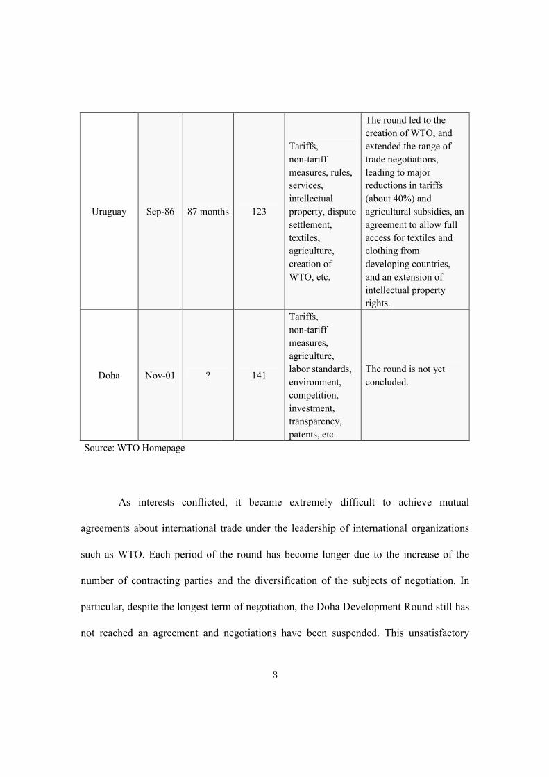
these negotiations have achieved desirable outcomes in the global economy. The long

series of trade negotiations and the achievements (including in the GATT and WTO

rounds) are presented in Table 1.

1 The Great Depression and Economic Nationalism (2008). In Revision Notes.Co.Uk. Retrieved from October 20, 2008, from: http://www.revision-notes.co.uk/revision/33.html 2 General Agreement on Tariffs and Trade. The Activities of GATT 1960/61. (1961), Geneva, Switzerland: Author.

2

Table 1: GATT and WTO Trade Rounds

�ame Start Duration Countries Subjects

covered Achievements

Geneva Apr-47 7 months 23 Tariffs

Signing of GATT,

45,000 tariff concessions

affecting $10 billion of

trade

Annecy Apr-49 5 months 13 Tariffs

Countries exchanged

some 5,000 tariff

concessions.

Torquay Sep-50 8 months 38 Tariffs

Countries exchanged

some 8,700 tariff

concessions, cutting the

1948 tariff levels by

25%.

Geneva II Jan-56 5 months 26

Tariffs,

admission of

Japan

$2.5 billion in tariff

reductions

Dillon Sep-60 11 months 26 Tariffs

Tariff concessions worth

$4.9 billion of world

trade

Kennedy May-64 37 months 62 Tariffs,

Anti-dumping

Tariff concessions worth

$40 billion of world

trade

Tokyo Sep-73 74 months 102

Tariffs,

non-tariff

measures,

"framework"

agreements

Tariff reductions worth

more than $300 billion

dollars achieved.

3

Uruguay Sep-86 87 months 123

Tariffs,

non-tariff

measures, rules,

services,

intellectual

property, dispute

settlement,

textiles,

agriculture,

creation of

WTO, etc.

The round led to the

creation of WTO, and

extended the range of

trade negotiations,

leading to major

reductions in tariffs

(about 40%) and

agricultural subsidies, an

agreement to allow full

access for textiles and

clothing from

developing countries,

and an extension of

intellectual property

rights.

Doha Nov-01 ? 141

Tariffs,

non-tariff

measures,

agriculture,

labor standards,

environment,

competition,

investment,

transparency,

patents, etc.

The round is not yet

concluded.

Source: WTO Homepage

As interests conflicted, it became extremely difficult to achieve mutual

agreements about international trade under the leadership of international organizations

such as WTO. Each period of the round has become longer due to the increase of the

number of contracting parties and the diversification of the subjects of negotiation. In

particular, despite the longest term of negotiation, the Doha Development Round still has

not reached an agreement and negotiations have been suspended. This unsatisfactory

4

outcome dramatizes the severity of the problem.

In this context, since the 1990s, countries have begun to make bilateral Regional

Trade Agreements (RTAs) as well as multilateral ones to create alternative trade

relationships without trade barriers such as tariffs and quotas. The commitment to

regionalism by the United States and European Community (EC), in particular, triggered

sharp increase of RTAs. Figure 1 clearly shows this recent change. In 1990, the total

number of RTAs was only 46, but this number increases to 213 in 2008 – nearly fivefold.

0

50

100

150

200

250

1948 1953 1958 1963 1968 1973 1978 1983 1988 1993 1998 2003 2008

Nu

mb

er

of

RTA

s

Year

Figure 1: Evolution of Regional Trade Agreement

in the World: 1949 – 2008

Cumulative active RTAsSource: WTO Homepage

One question that arises is whether there is any regional trend in this increase of

RTAs? Figure 2 compares the frequency of concluding RTAs in Asia, America, Europe,

5

and other regions. The figure shows Asian and African countries, as well as American and

European ones actively signed RTAs, and that signing RTA has now become a “world

trend” to achieve trade liberalization.

0

20

40

60

80

100

1957 1962 1967 1972 1977 1982 1987 1992 1997 2002 2007

Figure 2: Frequency of Concluding RTAs in Each Area

Asia Europe Americas Africa and OthersSource: WTO Homepage

Despite the recent predominant political support for RTAs, the actual trade effect

of RTAs is still in dispute. Many recent papers argue that RTAs bring countries certain

positive trade effects, but the research results are ambiguous because the trade effect of

RTAs is complicated and it has negative (trade diversion) effects as well as positive (trade

creation) effects. In addition, some analysts counter that the exceptional increase of RTAs

might impede the improvement of international free trade that is based on the WTO

agreements. International free trade maximizes the country’s profit in the global market in

6

the long run and it is the ultimate goal in global economy. If RTAs are really “stumbling

block” to this goal, it must be problematic for the future of international economy.

This study examines the growth and impact of regional trade agreements. It first

attempts to explain the factors behind the recent increase in RTAs. Using trade and

geographic data from some public datasets (trade dataset created by Professor Andrew K.

Rose and historical dataset created by Freedom House) and multivariate analyses

including the gravity model, I estimate the impacts of RTAs on their members’ annual

trade volume. Earlier research has focused specific RTAs such as North America Free

Trade Agreement (NAFTA) and EC, but this work has not covered all of the RTAs. Given

the sheer number of such agreements, it seems a more comprehensive analysis is

warranted, covering as well the overall effect of RTAs on the trade, economies, and

societies of participating countries.

7

Chapter II: Background

An RTA is a regional agreement that is provided for in GATT and the General

Agreement on Trade in Services (GATS) as an exception to the Most-Favored-Nation

(MFN) Principle3. WTO cites three types of RTAs: (1) Free Trade Areas and Customs

Unions that are based on paragraph 4 to 10 of Article XXIV of GATT; (2) Preferential

Trade Arrangements that are based on “Enabling Clause”; and (3) Economic Integration

that is based on Article V of GATS4. I discuss each one below.

(1) Free Trade Areas and Customs Unions

A free trade area is “a group of two or more customs territories in which the

duties and other restrictive regulations of commerce are eliminated on substantially

all the trade between the constituent territories in products originating in such

territories.5” The European Free Trade Association (EFTA), NAFTA, and Central

European Free Trade Agreement (CEFTA) are the representative examples reported

to WTO.

A customs union is “the substitution of a single customs territory for two or

3 The definition of MFN principle is as follows: “Under the WTO agreements, countries cannot normally discriminate between their trading partners. Grant someone a special favour (such as a lower customs duty rate for one of their products) and you have to do the same for all other WTO members.” (Principles of the trading system (2008). In WTO Homepage. Retrieved from October 20, 2008: from http://www.wto.org/english/theWTO_e/whatis_e/tif_e/fact2_e.htm) 4 WTO Homepage (2008) 5 GATT XXIV 8(b)

8

more customs territories”6. It is the same as a free trade area in eliminating the

restrictive regulation of commerce such as tariffs and quotas. However, each member

of the union has to apply “the same duties and other regulations of commerce to the

trade of territories not included in the union”7. That is, a customs union is less trade

restrictive to the countries outside of the union members than a free trade area. The

representative examples of a customs union are EC, the Central American Common

Market (CACM), and MERCOSUR.

(2) Preferential Trade Arrangements

A preferential trade arrangement is a group of two or more customs territories

eliminating restrictive regulations. Such arrangements have applied to developing

countries in particular, and are provided for in the 1979 GATT Decision on

Differential and More Favorable Treatment, Reciprocity and Fuller Participation of

Developing Countries, called the “Enabling Clause”. Considering the disadvantage

of developing countries about trade competition, the conditions to sign a preferential

trade arrangement are relatively looser than free trade areas and customs unions. The

Latin American Integration Association (LAIA）and the Common Market for Eastern

and Southern Africa (COMESA) are the representative examples of this type of RTA

reported to WTO.

6 GATT XXIV 8(a) 7 GATT XXIV 8(a)

9

(3) Economic Integration

Compared to other RTAs, an economic integration has a different perspective in

terms of trade facilitation. It focuses on the liberalization of trade in services. Most

economic integrations reported to WTO are existing free trade areas and customs

unions that expand its focus of trade facilitation from commodities to services. EC,

NAFTA, and CEFTA are examples of this type of RTA.

Table 2 indicates the total number of each type of RTA. The largest number of

RTAs is free trade areas, economic integration is second.

Table 2: Total �umber of Each RTA Reported to WTO by 2008

GATT Art. XXIV Enabling Clause GATS Art. V Total

Free Trade Area Customs Union

131 19 26 56 213

Source: WTO Homepage

10

Chapter III: Literature Review

Much previous research has tried to construct theoretical and empirical models

that illuminate the channels through which RTAs affect the domestic and international

economy. These studies cover diverse ideas and interact with each other in complex ways,

but some researchers such as Panagariya (2000) and Endo (2005) describe and arrange

them. I categorize previous research into two groups – theoretical studies analyzing the

effects of RTAs on economic welfare, and empirical studies analyzing the effects of RTAs

on trade amounts.

(1) Theoretical Approach

a. Effects of RTA on Economic Welfare

The traditional research illuminates the economic effects of RTAs on their

members. The most highly regarded theories concern trade creation and trade

diversion effects (Viner 1950). The Trade creation effect is the new trade that

RTAs bring members; this is driven by the elimination of tariffs. RTAs eliminate

tariffs in the area and stimulate community trade among members, so the

members that can import the cheaper goods from other members as a result of

tariff elimination increase economic welfare. The trade diversion effect is that

RTAs cause an ineffective trade situation and decrease profits in the area. That is,

RTAs only eliminate tariffs in the limited area members and create a

11

discriminatory trade situation. As a result, primarily higher-cost products made

in member countries are supplied rather than cheaper ones made in non-member

countries, and in the end the total economic welfare decreases. Viner indicates

that the total economic effects of RTAs would be measured by the sum of those

two effects. Viner’s idea triggered the invention of new RTA theories, which are

more consistent with real situations, but are also more complicated, as shown by

later research (Lipsey 1957; Michaely 1965; Bhagwati 1971).

b. Long Run Effects of RTA on World Trade

Along with the study of the short-term effect of RTAs, many researchers

have also discussed what the RTAs bring the world as well as each country in the

long run. These arguments fall in two groups: one regards the RTA as a “building

block” for achieving global trade liberalization; the other regards it as a

“stumbling block”. On the building block side, Baldwin (1995) proposes the

“domino effect” theory that the reduction of international trading costs due to

trade liberalization for those signing the RTAs increases the relative costs of

non-members and encourages them to join the agreement.

On the other side, Bhagwati (1998) proposes a “spaghetti bowl” theory and

expresses the concern that RTAs have the possibility of becoming stumbling

block to achieving free trade in the world. Bhagwati suggests that many

countries conclude different RTAs that provide different rules of origin, and

12

trade procedures becomes quite complicated like a spaghetti bowl. This has a

negative overall effect on trade and the global economy.

(2) Empirical Approach

Compared to theoretical studies, the content and methods of empirical studies of

RTAs are more straightforward. Most papers use the same method to analyze the

change in trade volume using a gravity model. The gravity model applies Isaac

Newton’s Law of Universal Gravitation to the empirical study of international

economics. Newton’s idea is that the gravitational attraction between two objects is

directly proportional to the product of their masses and inversely proportional to the

square of their distance. In the gravity model of international trade, the theory of

gravitational attraction between two objects is applied to the bilateral trade flows

between the “economic mass” of two countries. Rose (2003) analyzes the trade effect

on countries brought by the accession to General Agreement on Tariffs and Trade

(GATT) and concludes that GATT accession is not statistically significant in

increasing the trade flows.

Meanwhile, Goldstein, Rivers, and Tomz (2005) study the same research

question as Rose, but they add new variables, institutional standing and institutional

embeddedness, to the model. And they reach a totally opposite result; they conclude

that GATT accession has a remarkable effect on trade flows. The gravity model is

used not only for analyzing the effect of international institutions such as GATT and

13

WTO but also for the multilateral agreements such as RTAs. Coulbaly (2007)

analyzes seven RTAs in Africa, Asia, and Latin America and concludes that all have a

positive impact on their trade members.

This study focuses mainly on the empirical approach, but it expands upon

existing research in two key ways. First, my dataset covers all RTAs up to 2000 as well as

representative RTAs examined by earlier studies. Second, in addition to the gravity model,

I use some multivariate analyses to clarify the factors encouraging countries to conclude

RTAs and examine the effect of concluding RTAs on each country’s annual trade amount.

These refinements will contribute to deciding whether the overall effect of RTAs on trade

is positive or not. Are RTAs a building block or stumbling block to achieving future

economic progress?

14

Chapter IV: Conceptual and Empirical Model

(1) Conclusion of an RTA

I begin by evaluating a country’s decision to sign an RTA. This first-stage model

is composed of two assumptions. The first assumption is that a country’s

demographic, economic, and social changes have an influence on the decision to

conclude an RTA. Although my main interest in this thesis is to analyze the effect of

concluding RTA on international trade, it is essential to first examine which factors

are correlated with the decision of concluding RTAs. This is because countries that

conclude RTAs may be systematically different that those who do not conclude RTAs,

leading to a biased estimate on trade volume. For example, suppose that countries

concluding RTA are more likely to engage in trade regardless – and so have more

open, dynamic economies. In this case, my results will be biased upwards.

Essentially I would be estimating the effects of RTA and a country’s underlying

openness to trade. This first-stage allows me to predict the likelihood that any one

country would conclude an RTA.

Then, I estimate a fitted value of RTA dummy variable and analyze my main

analysis using Two Stage Least Squares (2SLS) estimation. That is, I regard the

decision to conclude an RTA as an endogenous variable and estimate a “first stage”

equation to generate a fitted value of the endogenous variable that is purged of error.

Then, I use a fitted value of the independent variable in “second stage” equation of

15

interest. My dependent variable, a dummy variable that is an indicator of concluding

RTAs, is assumed to be a function of three factors – economic situation, geographic

situation, and political situation. Regarding the first stage regression, my hypothesis

is that better economic, geographic, and political indicators raise the likelihood of

concluding RTAs.

The second assumption is that a country’s demographic, economic, and political

changes also have an influence on the number of concluded RTAs. I change the

dependent variable from the RTA dummy to the number of concluded RTAs in each

country. The hypothesis is that with an improvement of economic, geographic, and

political indicators, the number of concluding RTAs increases. I also use the fitted

value of the dependent variable to examine the 2SLS estimation in the second-stage

model.

(2) Economic Impact of RTA

The second-stage model is composed of two assumptions. The first assumption

is that the different country groups that are based on the likelihood of concluding an

RTA have different influences on the international trade amount. Through estimating

the “first stage” equation in the first model, I can estimate the fitted value of RTA

dummy, and it indicates the likelihood of concluding an RTA, purged of association

with other variables. Using the fitted value, I classify the countries into three groups.

Then, I focus on the group of the highest likelihood of concluding an RTA and

16

examine the differences of changes of trade amount according to whether the

countries concluded an RTA or not. The hypothesis is that country groups that

concluded RTAs show higher increases in trade amounts than groups that has never

concluded RTAs.

The second assumption is that any surge to in the trade amount in a country is

influenced by the increase of the number of concluded RTAs. In this assumption, my

analysis focuses more on the relationship between the trade amount and the effect of

concluding an RTA. I analyze two types of regression equation. The first regression

equation is a 2SLS model. My dependent variable is the mean of the total amount of

annual trade, and the independent variables are the fitted value of the RTA dummy,

the fitted value of the number of concluded RTAs in each country, and some

economic, geographic, and social indicators. I set up three hypotheses: (1)

concluding RTAs is positively correlated with increases in the trade amount; (2) with

an increase of total number of concluded RTAs, each country’s annual trade amount

increases; and (3) with an improvement of economic, geographic, and social

indicators, each country’s annual trade amount increases.

In the second regression equation, I focus on the bilateral trade relationships and

use the gravity model. That is, my dependent variable is the total amount of a

bilateral trade amount between the countries. Also, I include independent variables

that indicate former colonial relationship between trade partners beside the distance

between the countries, and economic, geographic, and social indicators. The

17

hypothesis is that, as in the first regression, with an increase of concluded RTAs, the

trade amount increases.

Figure 3 depicts all of my assumptions, the complex relationships among factors

effecting trade , and my analytic methods.

Dummy of

concluding RTAs

Number of

concluding RTAs

Trade Amount

Political rights

Civil liberties

Social factor

Population

Geographic factor

GDP per capita

Economic factor

First-Stage Model

Second-Stage Model

Analytic

method

Probit Model

Tobit Model

2SLS Model

Pooled OLS Model

Fix effect Model

Figure 3: Conceptual Framework

Distance

Colonial relationship

Otherfactors*

* I add these factors only in the gravity model

(3) Empirical Methods and Specification

Estimating equations I examine in this study are as follows:

18

a. First-stage model

First, I use a probit model to estimate the influence of each country’s

demographic, economic and social changes on the decision to conclude RTAs.

The dependent variable is a dummy variable that is an indicator of concluding

RTAs. Because the dependent variable is a dummy variable, Ordinary Least

Squares (OLS) Regression is not appropriate. The independent variables are

economic, geographic, and political indicators. I use a continuous variable for

real GDP per capita as an economic indicator and use a continuous variable for

population as a geographic indicator.

Next, I create a dummy variable for political rights and civil liberties in the

first dataset. Freedom House assesses each country’s political rights and civil

liberties on a scale from 1 (most free) to 7 (least free). Hence, I create two sets of

seven dummy variables for both political rights and civil liberties respectively.

For example, pr1 is a binary variable that is one if the political rights of the

country is 1 (most free), and zero otherwise. On both the political rights and civil

liberties scales, 1 (most free) was the most frequent condition in the dataset, so I

set 1 as a baseline and omitted the variable from the model.

I expect that population and GDP per capita will have positive impacts on

the dummy variable for concluded RTAs. And I expect the dummy variables

about political rights and civil liberties to show different effects according to

improving political rights and civil liberties. That is, the better political rights

19

and civil liberties become, the larger the positive impact on the dummy variable

for concluded RTAs. The specification of the estimated equation is:

rtas = β0 + β1ldefp1 + β2ldefy1 + β3pr2 + β4pr3+ β5pr4 + β6pr5 + β7pr6

+ β8pr7 + β9cl2+ β10cl3+ β11cl4+ β12cl5+ β13cl6 + β14cl7 … (1)

* “βx” or “γx” indicate estimated values of coefficients (the rest is the

same as above).

Second, I use a Tobit model to examine the influence of each country’s

demographic, economic, and social changes on the number of concluded RTAs.

The dependent variable is a number of concluding RTAs in each country.

Because the dependent variable has quite a lot of zeros as a minimum value in

the dataset, it is not proper to run an OLS regression. I use the same independent

variables as equation (1)

My dataset is panel data, so I estimate not only the usual Tobit model but

also the random-effects Tobit model. The usual Tobit model is mainly used for

cross sectional data, so the random-effects Tobit model is more suitable analytic

method to examine a panel data.

I expect the same direction of results as equations (1). That is, that

population and GDP per capita will have a positive impact on the number of

concluded RTAs. And I expect the dummy variables about political rights and

20

civil liberties to show negative effects on the number of concluded RTAs. The

specification of the estimated equation is:

numrtas = β0 + β1ldefp1 + β2ldefy1 + β3pr2 + β4pr3+ β5pr4 + β6pr5 + β7pr6


b. Second-stage model

First, I calculate the predicted value of the RTA dummy and classify the

countries according to this predicted value. In addition, I divide each group into

two subgroups: the group of countries that have concluded RTAs and the group

of countries that have never concluded RTAs. Then, I examine the difference in

changes of trades in the groups at three points in time, 1990, 1995, and 2000.

Second, using the fitted value of the RTA dummy and number of RTAs that

are calculated in the first model, I estimate 2SLS estimation. The independent

variables are population, real GDP per capita, fitted value of RTA dummy, and

fitted value of number of concluded RTA. I expect that all independent variables

to have a positive impact on the annual trade amount. The specification of the

estimated equation is:

lrtrade = β0 + β1ldefp1 + β2ldefy1+ β3(fitted value of rtas)

+β4(fitted value of numrtas) … (3)

21

Fitted value of rtas = γ0 + γ1ldefp1 + γ2ldefy1 + γ3pr2 + γ4pr3+ γ5pr4

+ γ6pr5 + γ7pr6+ γ8pr7 + γ9cl2+ γ10cl3+ γ11cl4

+ γ12cl5+ γ13cl6 + γ14cl7

Fitted value of numrtas = γ0 + γ1ldefp1 + γ2ldefy1 + γ3pr2 + γ4pr3+ γ5pr4

+ γ6pr5 + γ7pr6 + γ8pr7 + γ9cl2+ γ10cl3+ γ11cl4

+ γ12cl5+ γ13cl6 + γ14cl7

Third, I use three types of regression to estimate the gravity model: a Pooled

OLS model, a one-way fixed effect model, and a two-way fixed effect model. I

have to run the fixed effect model because I use a panel dataset and I cannot

ignore the fixed effect for the countries and the fixed effect for year. The

dependent variable is the mean of exporter’s trade amount to importer and

importer’s trade amount from exporter for each pairing of 81 countries.

I basically add the same economic, geographical, and social indicators: both

exporter and importer’s population and real GDP per capita, and dummy

variables for political rights in exporting country. But I also add the distance

between countries and the dummy variables that indicate the former colonial

relationship to analyze the gravity model. I expect the same direction of results

as equations (1) through (3). That is, that population and GDP per capita will

have a positive impact on the annual bilateral trade amount, and the better the

22

political rights and civil liberties become, the more the annual bilateral trade

amount becomes. I assume that the RTA dummy indicates a positive relationship

with the annual bilateral trade amount. In addition, the former colonial

relationship shows a close relationship between the countries, so I assume that

the dummy variables related to the colonial history have a positive relationship

with the annual bilateral trade amount. The specification of the estimated

equation is:

lrx1to2 = β0 +β1gw1 +β2gw2 + β3regional+ β4dist + β5pr2 + β6pr3+ β7pr4

+ β8pr5 + β9pr6 + β10pr7 + β11ldefy1+ β12ldefy2 + β13ldefp1

+ β14ldefp2+ β15border + β16colony + β17comcol+ β18curcol … (4)

23

Chapter V: Data

(1) Datasets

This study is conducted using the datasets I constructed from two

publicly-available datasets. The first data source is the trade dataset created by

Professor Andrew K. Rose. In 2003, Rose made the dataset using the data from the

International Monetary Fund and Central Intelligence Agency data, and he used this

dataset to examine the causality between membership in WTO or GATT and the

stability of trade flows. This dataset is public in his website8. It covers bilateral

merchandise trade between 178 IMF trading entities between 1957 and 2000. In this

massive amount of data, I focus on the data that is directly related to my study. That is,

I choose 81 countries that have concluded over three RTAs. (The Appendix tabulates

the countries covered in my dataset.) Then, I sum each country’s bilateral trade

amount and change Rose’s annual bilateral trade data to individual country’s annual

trade data. Rose’s dataset also has basic economic and geographic variables such as

GDP per capita and population.

What that dataset does not provide is information on social indicators, which I

need to examine the RTA decision. I add some variables that indicate each country’s

political and social stability from historical data of Freedom House. Freedom House

is an independent non-governmental organization that conducts research and

8 Available from: http://faculty.haas.berkeley.edu/arose/RecRes.htm

24

advocacy on democracy, political freedom and human rights. It has published an

annual assessment of the perceived degree of democratic freedom in each country

since 1972, which is used in political science research. I use the data on the civil and

political rights in my selection of 81 countries since 1972. As a result, I make two

datasets. The first one is individual country’s trade dataset that contains economic,

geographic, and political information. The second dataset is a bilateral trade dataset

that contains both exporter and importer’s economic, geographic, and political

information. My datasets cover 81 countries’ annual trade amounts, as well as

geographic, economic, and political data between 1972 and 2000.

(2) Variables

The first dataset has two variables to indicate each country’s record of concluded

RTA: a dummy variable that is an indicator of concluded RTAs and a number of

concluded RTAs in each country. Also, the first dataset has economic, geographic,

and political indicators: mean of annual real trade amount, real GDP per capita,

population, and dummy variables for political rights and civil liberties. I deflate GDP

per capita and trade amounts by the American Consumer Price Index for all urban

consumers (1982-1984 = 100).

The second dataset has a dummy variable that is an indicator of concluded RTAs.

This dataset also has economic, geographic, and political indicators: annual bilateral

trade amount, both exporter and importer’s real GDP per capita and population, and

25

dummy variables for political rights, In addition, this dataset has the distance

between countries, the dummy variables for land border, and the dummy variables

that indicate the former colonial relationship. There are three types of former colonial

relationship variables: Dummy for pairs ever in colonial relationship, dummy for

common colonizer post 1945, and dummy for pairs currently in colonial relationship.

The same as the first dataset, I deflate trade amounts and GDP per capita by the

American Consumer Price Index for all urban consumers.

Tables 3 and 4 show the descriptive statistics for the variables in the two models.

The tables show 68.1% of the country-year observations had an RTA, with an

average 2.678 RTA concluded in those countries that had one. The maximum number

of concluding RTA was 21 by Belgium, France, Luxemburg, and Netherland.

Table 3: Descriptive Statistics of Analysis Variables (First Dataset)

Variables Description Obs Mean Std. Dev.

rtas Dummy for concluding RTAs 1,746 0.681 0.466

lrtrade logarithm of mean of real trade amount 1,746 14.71 1.676

ldefy1 Logarithm of country's real GDP per capita 1,746 9.475 0.652

ldefp1 Logarithm of population 1,746 9.29 1.723

pr1 Political rights = 1 (the highest degree of

freedom) 1,673 0.692 0.462

pr2 Political rights = 2 1,673 0.107 0.309


26




pr7 Political rights = 7 (the lowest degree of

freedom) 1,746 0.022 0.148

cl1 Civil liverties = 1 (the highest degree of

freedom) 1,675 0.518 0.5

cl2 Civil liverties = 2 1,675 0.233 0.423





cl7 Civil liverties = 7 (the lowest degree of

freedom) 1,675 0.013 0.113

numrtas Total number of RTAs each country concluded 2,499 2.678 3.996

Table 4: Descriptive Statistics of Analysis Variables (Second Dataset)

Variables Description Obs Mean Std. Dev.

lrx1to2 Logarithm of mean of trade from exporter to

importer 106,564 11.826 3.189

Year Year (1972 - 2000) 106,564 1987.604 8.509

gw1 Exporting country in GATT/WTO 106,564 0.793 0.405

gw2 Importing country in GATT/WTO 106,564 0.715 0.451

regional2 Dummy for RTAs 106,564 0.0739 0.262

Ldist Logarithm of distance between exporting

and importing countries 106,564 7.967 0.941

pr1 Exporter's political rights = 1 (the highest

degree of freedom) 106,564 0.463 0.499

pr2 Exporter's political rights = 2 106,564 0.131 0.337

27





pr7 Exporter's political rights = 7 (the lowest

degree of freedom) 106,564 0.051 0.221

ldefy1 Logarithm of exporting country's population 106,564 8.965 0.85

ldefy2 Logarithm of importing country's population 96,093 8.954 0.862

ldefp1 Logarithm of exporting country's real GDP

per capita 106,564 9.569 1.693

ldefp2 Logarithm of importing country's real GDP

per capita 96,223 9.444 1.725

border Dummy for land border 106,564 0.34 0.181

colony Dummy for pairs ever in colonial

relationship 106,564 0.023 0.149

comcol Dummy for common colonizer post 1945 106,564 0.406 0.197

curcol Dummy for pairs currently in colonial

relationship 106,564 0.001 0.03

28

Chapter VI: Results

(1) First-stage model

I begin with a discussion of relationship between the conclusion of an RTA and a

country’s economic, geographic, and political indicators.

rtas = β0 + β1ldefp1 + β2ldefy1 + β3pr2 + β4pr3+ β5pr4 + β6pr5 + β7pr6


Table 5 shows the results of the probit model. The main factor explaining a

country’s decision to enter into an RTA is political rights. All dummies covering the

entire range of political right (except for free countries) are negative, meaning that the

highest degree of political rights lead to the highest likelihood of concluding RTAs. In

addition, as the degree of political rights becomes lower, the coefficient of political

rights also becomes lower. For example, when the country’s degree of political rights

is 2(the second highest), the coefficient is -0.199. However, the degree of political

rights is 7(the lowest), the coefficient is -0.502. I conducted hypothesis testing to

confirm whether the difference between these coefficients is insignificant. The

T-statistic is 12.86 and it rejects the null hypothesis. That is, the change of coefficient

is statistically significant. These results indicate that weak political rights are an

obstacle to trade, in particular to concluding RTAs.

29

Other variables seem to have much less of an impact. Population and GDP per

capita have no statistically significant effect on a country’s decision to enter into an

RTA, as do measures most measures of civil liberties. The exception with civil

liberties is 4 or 6. I assume the same relationships as a case of political rights – i.e. the

restriction of civil liberties is negatively correlated with the likelihood of concluding

RTAs: so the result goes against my expectation. It is also worth noting the difference

between the coefficients of the variables for the degree of civil liberties, cl2 and cl7,

is not statistically significant (T-statistics = 1.00). That is, the degree of civil liberties

does not have a significant impact on the decision to conclude RTAs.

Table 5: Coefficients of Probit Model Analyzing the Effect of Economic,

Geographic, and Political Indicators on Concluding RTAs

Probit Model

Log Real GDP per capita 0.025 (0.025)

Log population -0.002 (0.008)

Political Rights:

High 2 -0.199*** (0.053)

3 -0.199*** (0.080)

4 -0.245*** (0.080)

5 -0.432*** (0.067)

6 -0.443*** (0.068)

Low 7 -0.502*** (0.063)

30

Civil liverties:

High 2 -0.043 (0.045)

3 -0.027 (0.072)

4 -0.194*** (0.083)

5 -0.105 (0.092)

6 -0.215*** (0.104)

High 7 0.080 (0.123)

Pseudo R-square 0.183

Dependent variable: dummy for concluding RTAs

Number of Observations = 1,673

*** : significant at 0.01 level ** : significant at 0.05 level

* : significant at 0.1 level

Next, I examine the relationship between the number of concluded an RTA and a

country’s economic, geographic, and political indicators.

numrtas = β0 + β1ldefp1 + β2ldefy1 + β3pr2 + β4pr3+ β5pr4 + β6pr5 + β7pr6


Table 6 shows the results for the two types of Tobit models. The first column of

the table 6 indicates the result of usual Tobit model. Almost all of the variables are

statistically significant at the 0.01 level. GDP per capita has the expected positive

effect; a one percent increase of GDP per capita raises the number of concluded

RTAs by 5.3%, Population, however, does not correspond with my expectation that it

31

encourages RTAs; the result shows that a one percent increase in population reduces

the number of concluding RTAs by 0.2%. Next, the coefficients of political rights

indicate the same results as in the discrete decision to enter into an RTA. That is, all

of the coefficients of political rights are negative and as the degree of political rights

becomes lower, the coefficient of political rights also becomes lower. In addition, the

difference between the coefficients between of the variables for degrees of political

rights, pr2 and pr7 is statistically significant at 0.01 level (T-statistics = 2.42). The

coefficients of civil liberties except cl6 are statistically significant and the difference

of coefficients between cl2 and cl7 is statistically significant at 0.1 level (T-statistics

= 1.82). I assume these coefficients show the same trend as political rights so this

result goes against my assumption. One reason why such differences may occur may

be if civil liberties are more directly connected with people’s daily lives than political

rights, and restriction of civil liberties encourages people to desire their freedom

more rather than only hinder them.

The second column of Table 6 indicates the result of the random-effects Tobit

model. The results basically have the same tendency as the first column’s results and

except for civil liberties fit with my assumption. One big change in this model is that

the coefficient of the logarithm of population turns positive and fits with my

assumption.

32

Table 6: Tobit Model and Random-effects Tobit Model Analyzing the Effect of Economic,

Geographic, and Political Indicators on the Total �umber of Concluding RTAs

Model 1

Tobit model

Model 2

Random-effects

Tobit Model

Log Real GDP per capita 5.295*** (0.349) 7.254*** (0.357)

Log population -0.187*** (0.079) 1.066*** (0.297)

Political Rights:

High 2 -3.595*** (0.517) -1.992*** (0.348)

3 -1.725 (1.158) -1.968*** (0.503)

4 -2.362** (1.205) -1.790*** (0.536)

5 -6.134*** (1.384) -2.593*** (0.611)

6 -6.554*** (1.411) -2.466*** (0.628)

Low 7 -7.910*** (2.063) -3.128*** (0.786)

Civil liverties:

High 2 3.187*** (0.348) 1.011*** (0.296)

3 3.291*** (0.712) 1.460*** (0.458)

4 1.938* (1.144) 1.112** (0.564)

5 3.748*** (1.295) 2.026*** (0.603)

6 2.071 (1.648) 2.320*** (0.744)

Low 7 7.269*** (2.269) -0.515 (1.167)

Psuedo R2 0.120 -

Dependent variable: Total number of concluding RTAs


*** : significant at 0.01 level ** : significant at 0.05 level * : significant at 0.1 level

(2) Second-stage model

In the second model, I first divide all data into three groups according to the

33

distribution of the predicted value of the dependent variable rtas in the first model.

Figure 4 shows the result of group allocation. I make Groups 1 and 2 according to

each quartile. Third and fourth quartiles, however, show similar predicted

probabilities, so I combine these quartiles and make Group 3. Group 1 shows the

lowest likelihood for concluding RTAs, Group 2 is in the middle, and Group 3 shows

the highest likelihood of concluding RTAs.

Figure 4: Distribution of Predicted Value of rtas

Percentiles rtas^

Range Group name

1% 0.119

rtas^ < 0.342 Group 1

5% 0.187

(bottom quartile)

25% 0.342 0.342=<rtas^<0.616 Group 2

50% 0.616 (next quartile)

75% 0.824

rtas^=> 0.616 Group 3

99% 0.839

(top half)

Next, I examine each group’s change of average real amount of trade in 1990,

1995, and 2000. Table 7 shows the number of countries in each group and groups 1

and 2 are too few to examine the change of average real trade amount. Hence, I focus

on Group 3: the group of the highest likelihood of concluding an RTA.

34

Table 7: �umber of Observations in Each Country Group

Number of Observations

1990 1995 2000

Non

RTA RTA

Non

RTA RTA

Non

RTA RTA

Group 1 12 1 6 5 3 10

Group 2 6 8 11 10 1 12

Group 3 8 23 13 26 5 39

Tables 8 and 9 show the result. Table 8 focuses on the change of trade amount in

Group 3 according to whether the countries concluded RTAs or not. In Group 3,

countries concluding RTAs show a higher amount of trade than non-concluding

countries in all three periods. This result suggests that concluding RTAs has a

positive economic impact on countries and the higher the likelihood of concluding

RTAs is, the more economic benefits countries can get. It fits with my assumption.

Table 8: Change of Average Real Amount of Trade in Group 3

(Between the Countries That Did �ot Conclude RTA and That Concluded

RTA: 1990, 1995, and 2000)

M e a n o f r e a l t r a d e a m o u n t (U S $)

1990 1995 2000

Non RTA RTA Non RTA RTA Non RTA RTA

6,044,220 9,555,227 3,706,371 8,248,925 2,719,955 7,952,153

n = 8 n = 23 n = 13 n = 26 n = 5 n = 39

Table 9 also supports this suggestion. Table 9 compares the growth rate of the

35

average trade amount of all peer of countries in group 3 according to the status

whether to conclude RTAs or not. The table does not necessarily show the expected

result; the average trade amount of country group in which concludes RTAs steadily

decreases during the three periods. The countries that conclude RTAs experience a

14% decline in trade between 1990 and 1995, and a 3% decline between 1995 and

2000. Nevertheless, compared to the non-concluding countries, countries that

conclude RTAs show significant effects on the growth of trade amounts.

Non-concluding RTA countries show a decline of -39% between 1990 and 1995 and

-27% between 1995 and 2000. That is, the growth rate of non-concluding RTA

countries is even more negative growth rate. Thus, concluding RTAs seems to ease

the negative economic impact on countries and it indirectly supports the potential

positive economic effect of RTAs.

Table 9: Change of Average Real Amount of Trade in Group 3

(Between the Countries that Did �ot Conclude RTA and That Concluded RTA:

1990, 1995, and 2000)


N o n R T A

1990 1995 Growth from 1990 2000 Growth from 1995

6,044,220 3,706,371 -39% 2,719,955 -27%

n = 8 n = 13 n = 5

36


R T A

1990 1995 Growth from 1990 2000 Growth from 1995

9,555,227 8,248,925 -14% 8,028,139 -3%

n = 23 n = 26 n = 39

Next, I ran the 2SLS model to examine the effects on trade amounts of

concluding RTAs, the number of concluded RTA, population, GDP per capita, and

population.

lrtrade = β0 + β1ldefp1 + β2ldefy1+ β3(fitted value of rtas)

+β4(fitted value of numrtas) … (3)

Table 10 shows the result. All independent variables are statistically significant

at 0.01 levels. GDP per capita and population has a positive effect on trade and these

results fit with my assumption. Interestingly, concluding RTA is associated with the

decrease of trade amount by 4.5% and it goes against my assumption. I assume this

result indicates that concluding RTA is necessary condition to achieve economic

development but it does not necessarily guarantee the development. The more

important factor for the country’s economic progress might be how to exploit RTA’s

economic benefit. On the other side, a one-point increase of the total RTA number is

associated with the increase of trade amount by 9.9%. This result indicates the

37

importance of increasing RTA partners to develop trade and fit with my assumption..

Table 10: Two-stage Least Square (2SLS) Model Analyzing the Effect of Concluding

RTAs, �umber of Concluded RTAs, and Economic and Geographic Indicators

on Trade Amounts

2SLS Model

Log Real GDP per capita 1.275*** (0.049)

Log population 0.692*** (0.011)

Dummy for concluding RTA (Predicted value) -0.454*** (0.120)

Number of Concluding RTAs (Predicted value) 0.099*** (0.028)

R-square 0.873

Dependent variable: Logarithm of mean of trade amounts



Finally, I examine the gravity model using the bilateral trade dataset.

lrx1to2 = β0 +β1gw1 +β2gw2 + β3regional+ β4dist + β5pr2 + β6pr3+ β7pr4

+ β8pr5 + β9pr6 + β10pr7 + β11ldefy1+ β12ldefy2 + β13ldefp1

+ β14ldefp2+ β15border + β16colony + β17comcol+ β18curcol … (4)

Table 11 presents the results. The first column shows the result of Model 1, the

38

pooled OLS model. All of the independent variables are statistically significant at

0.01 level. GDP per capita and population are positively correlated with the trade

amount and all political rights variables are negatively correlated with it. These

results are consistent with the analyses in my first model. In addition, if the exporting

country has concluded an RTA with the importing country, the trade amount will

increase by 18.4%. This result also supports my assumption.

The second and third columns show the result of Models 2 and 3, one-way and

two-way fixed effect models. In these models I control fixed effect for each unit (i.e.,

country) and fixed effect for years. The results are basically same as Model 1. But

Model 3 shows more expected results. In Model 2 some variables such as exporter’s

GATT/WTO status, some political rights variables, and GDP per capita show totally

opposite results and I cannot find any plausible reason why this happens. In Model 3,

the coefficient of the RTA dummy is still significant at the 0.1 level which indicates

that concluding an RTA is associated with increase of trade amount by 3.2%. The

result supports my assumption that concluding RTAs has a positive effect on bilateral

trade amounts even after I control the country and year fixed effects.

Table 11: OLS Regression Coefficients for Models Analyzing the Effect of RTAs

on Exports

Model 1

Pooled OLS

Model2

One-way Fixed

Model3

Two-way Fixed

Exporter in

GATT/WTO 0.438*** (0.166) -0.013 (0.027) 0.036* (0.027)

39

Importer in

GATT/WTO 0.228*** (0.015) 0.170*** (0.014) 0.169*** (0.013)

RTA Dummy 0.184*** (0.022) 0.409*** (0.020) 0.032* (0.019)

Log Distance -0.928*** (0.007) -1.180*** (0.007) -1.190*** (0.007)

Political

Rights:

High 2 -0.128*** (0.020) 0.057*** (0.025) -0.167*** (0.026)

3 -0.243*** (0.026) -0.058** (0.033) -0.285*** (0.034)

4 -0.356*** (0.024) 0.332*** (0.030) -0.188*** (0.034)

5 0.142** (0.024) 0.070*** (0.033) -0.232*** (0.034)

6 -0.334*** (0.025) 0.132*** (0.034) -0.252*** (0.036)

Low 7 0.197*** (0.031) 0.355*** (0.040) -0.114*** (0.042)

Log Real GDP per

capita (Exporter) 1.588*** (0.010) 0.605*** (0.026) 1.200*** (0.032)

Log Real GDP per

capita (Importer) 1.356*** (0.008) 1.467*** (0.007) 1.481*** (0.028)

Log Population

(Exporter) 0.934*** (0.004) -0.957*** (0.050) 0.569*** (0.068)

Log Population

(Importer) 0.822*** (0.003) 0.852*** (0.003) 0.853*** (0.003)

Border 0.641*** (0.034) 0.267*** (0.036) 0.259*** (0.031)

Colony 1.310*** (0.038) 1.316*** (0.036) 1.305*** (0.036)

Common Colonizer 1.320*** (0.031) 1.416*** (0.028) 1.435*** (0.028)

Current Colony 0.848*** (0.269) 1.150*** (0.253) 1.153*** (0.250)

R-square 0.689 0.625 0.633

Dependent variable: Logarithm of mean of trade from exporter to importer



40

Chapter VII: Policy Implications and Conclusions

My results suggest the political environment has an important impact on trade

promotion. Specifically, I find that weak political rights reduce the likelihood that a

country enters into regional free trade agreements. This result is not surprising at some

level, and suggests that promoting stronger political rights is akin to promoting faster

economic growth. This result is important in a methodological sense as well, since it

suggests a need to model a country’s decision to enter into an RTA. Furthermore, both

political rights and civil liberties are correlated with the number of concluded RTAs.

Interestingly, however, deterioration of political rights is negatively correlated and

deterioration of civil liberties is positively correlated.

RTAs are found to have a strong positive effect on overall trade volume in

several different ways. First, comparing the average trade volume by countries’

likelihoods to enter into such agreements shows a positive effect of RTAs on trade.

Second, though RTA dummy is negatively correlated with the total annual amount of

trade, number of RTAs is positively correlated with it. Finally, the gravity model shows

that concluding RTAs is positively correlated with the annual total amount of exports and

former colonial relationship; and population and GDP are positively correlated with the

annual total amount of exports.

RTAs likely divert trade from some countries and change the overall pattern of

trade flows, but what this study shows is that they do raise the overall volume of trade.

41

Nonetheless there are some limitations worth noting. First, I only covered 81 countries’

data; I could not fully analyze the effect of RTAs on global trade. Second, I only use trade

data through 2000. The number of concluded RTAs has dramatically increased since 2000.

So if I could have added the trade data in 2001 and later years, I would have shown

results based on the newest trade situation. Third, I did not take into account the

differences among the types of RTAs. If I could analyze my models according to the

different types of RTAs such as free trade area, customs union, preferential trade

arrangement, and economic integration, I would have shown more interesting and useful

results. Nevertheless, my findings are meaningful in that they indicate a certain

relationship between concluding RTA and trade amount.

My findings clearly support the view that concluding RTAs leads to positive

impacts on a country’s economy, and that RTAs are a useful building block for the

country’s future economic progress. At the same time, however, my results suggest the

importance of improving the country’s political situation since this can facilitate more

trade agreements. Countries that achieve more political freedom have a higher likelihood

to conclude RTAs and achieve economic progress. The result indicates that development

policies that focus only on economic progress and undervalue the improvement of civil

rights may hinder economic progress in the long run. Securing people’s fundamental

rights such as political rights and civil liberties brings stability to the society and

encourages foreign businesses to invest in the market. My study also shows that countries

that have relatively low levels of civil liberties have a higher likelihood of concluding

42

RTAs. On the basis of this result, I assume that people in these countries really desire to

enjoy civil liberties including free economic activities. The government should not ignore

such people’s voices and must respond them as much as it can. This policy action seems

to be off track, but it really leads to future economic development.

43

Appendix: The list of countries that were objects of this study

Albania Japan

Algeria Jordan

Armenia Kazakhstan

Australia Korea

Austria Kyrgyz

Azerbaijan Latvia

Bahrain Lebanon

Belgium Lithuania

Bosnia and Herzegovina Luxembourg

Brunei Macedonia

Bulgaria Malaysia

Canada Malta

Chile Mexico

China Moldova

China-Hong Kong Morocco

China-Macao Netherland

Costa Rica New Zealand

Croatia Nicargua

Cyplus Norway

Czech Pakistan

Denmark Panama

Dominica Poland

Egypt Portugal

El Salvador Romania

Estonia Russia

Faroe Islands Singapore

Finland Slovak

France Slovenia

Georgia South Africa

Germany Spain

Greece Sri Lanka

Guatemala Sweden

Hondulas Switzerland

Hungary Syria

Iceland Thailand

India Tunisia

Indonesia Turkey

Ireland Turkmenistan

Israel Ukraine

Italy United Kingdom

United States

44

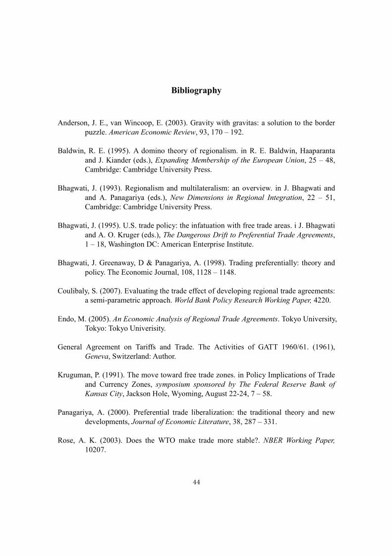
Bibliography

Anderson, J. E., van Wincoop, E. (2003). Gravity with gravitas: a solution to the border

puzzle. American Economic Review, 93, 170 – 192.

Baldwin, R. E. (1995). A domino theory of regionalism. in R. E. Baldwin, Haaparanta

and J. Kiander (eds.), Expanding Membership of the European Union, 25 – 48,

Cambridge: Cambridge University Press.

Bhagwati, J. (1993). Regionalism and multilateralism: an overview. in J. Bhagwati and

and A. Panagariya (eds.), &ew Dimensions in Regional Integration, 22 – 51,

Cambridge: Cambridge University Press.

Bhagwati, J. (1995). U.S. trade policy: the infatuation with free trade areas. i J. Bhagwati

and A. O. Kruger (eds.), The Dangerous Drift to Preferential Trade Agreements,

1 – 18, Washington DC: American Enterprise Institute.

Bhagwati, J. Greenaway, D & Panagariya, A. (1998). Trading preferentially: theory and

policy. The Economic Journal, 108, 1128 – 1148.

Coulibaly, S. (2007). Evaluating the trade effect of developing regional trade agreements:

a semi-parametric approach. World Bank Policy Research Working Paper, 4220.

Endo, M. (2005). An Economic Analysis of Regional Trade Agreements. Tokyo University,

Tokyo: Tokyo Univerisity.

General Agreement on Tariffs and Trade. The Activities of GATT 1960/61. (1961),

Geneva, Switzerland: Author.

Kruguman, P. (1991). The move toward free trade zones. in Policy Implications of Trade

and Currency Zones, symposium sponsored by The Federal Reserve Bank of

Kansas City, Jackson Hole, Wyoming, August 22-24, 7 – 58.

Panagariya, A. (2000). Preferential trade liberalization: the traditional theory and new

developments, Journal of Economic Literature, 38, 287 – 331.

Rose, A. K. (2003). Does the WTO make trade more stable?. &BER Working Paper,

10207.

45

Revision Notes.Co.Uk. (2008). The great depression and economic nationalism.

Available from: http://www.revision-notes.co.uk/revision/33.html

Viner, J. (1950). The customs union issue, New York: Carnegie Endowment for

International Peace.

World Trade Organization (2008). Principles of the trading systems. Available from:

http://www.wto.org/english/theWTO_e/whatis_e/tif_e/fact2_e.htm

THE EFFECT OF REGIONAL TRADE AGREEMENTS ON THE …

Documents

Transcript of THE EFFECT OF REGIONAL TRADE AGREEMENTS ON THE …