The Dynamics of Ultra-Thin Polymer Films in Different ... · verändert - die Viskosität ist um...
102
The Dynamics of Ultra-Thin Polymer Films in Different Confinements Studied by Resonance Enhanced Dynamic Light Scattering Dissertation zur Erlangung des Grades “Doktor der Naturwissenschaften” im Promotionsfach Physikalische Chemie am Fachbereich Chemie, Pharmazie und Geowissenschaften der Johannes Gutenberg-Universität Mainz Fan-Yen Lin geboren in Yi-Lan, Taiwan Mainz, April 2015
Transcript of The Dynamics of Ultra-Thin Polymer Films in Different ... · verändert - die Viskosität ist um...

The Dynamics of Ultra-Thin Polymer Films in
Different Confinements Studied by Resonance
Enhanced Dynamic Light Scattering
Dissertation
zur Erlangung des Grades
“Doktor der Naturwissenschaften”
im Promotionsfach Physikalische Chemie
am Fachbereich Chemie, Pharmazie und Geowissenschaften
der Johannes Gutenberg-Universität Mainz
Fan-Yen Lin
geboren in Yi-Lan, Taiwan
Mainz, April 2015


III
Abstract
The controversy about the glass transition on the nanoscale, e.g., the glass transition
temperature (Tg ) of polymer thin films, is not fully resolved. The nanoscale dynamic behavior is
strongly affected by the boundary conditions of the samples. Polymer thin films are ideal
systems to study the dynamics of polymer chains under different confinements, which I varied
in this thesis to gain more and better insight into this problem.
Resonance Enhanced Dynamic Light Scattering (REDLS) is a marker-free method and used to
investigate the dynamics of polymer thin film of which the dynamics of capillary wave is the
most prominent. Via the coupling of these to the mechanical properties of the film, e.g. the
dynamics of hidden layers, the confinement effects from the substrate can be studied.
Therefore, dynamics of thin, liquid polybutadiene (PB) films on solid substrates have been
studied at temperatures far above the glass transition temperature Tg. The capillary wave
dynamics are the stronger suppressed by the substrate, the thinner the film is. We find a
molecular weight independent film thickness below which the dynamics change dramatically –
the viscosity increases by orders of magnitude. This change is not related to 3Rg as postulated in
theory and claimed in some experimental findings, but rather to a fixed distance from the
polymer/glass interface. Part of our observations we attribute to a compared to bulk polymer less
mobile viscoelastic layer near the substrate, and part to a more mobile layer at the liquid- gas
interface. Thus, the overall behavior of the dynamics can be explained by a “three layer” model,
the third layer having bulk behavior in between the above two layers.
Second, polystyrene/polynorbornene (PS/PN) bilayers are measured at temperatures close to
Tg to observe the capillary wave of PS at the interface of PS/ PN. Because the capillary wave of
PS is strongly suppressed by the glassy PN layer, other modes of dynamic behavior are
accessible; they are vanishing in the noise, i.e. they are much smaller than the noise of the strong
capillary mode. The strongly suppressed capillary wave and a new mode found show Arrhenius,
i.e. thermally activated behavior above Tg which is an indication for strongly localized processes
or dynamical modes.
Third, the PS thin film is anchored to Au by thiol group in order to enhance the confinement
from the substrate. This creates artificially a less mobile layer and we gained insight into the role
of such a layer. In addition to the capillary wave, there is a local motion found existing at the
surface of PS thin film. Since the enhanced confinement from the substrate, the thickness of so-
called less mobile layer near the substrate is enlarged and makes the viscosity of the PS thin film
higher the bulk by half an order of magnitude. In my thesis I have shown how changing
confinement can influence the dynamics of polymer thin films.

IV
Zusammenfassung
Die Kontroverse über den Glasübergang im Nanometerbereich, z. B. die Glasübergangs-
temperatur Tg von dünnen Polymerfilmen, ist nicht vollständig abgeschlossen. Das dynamische
Verhalten auf der Nanoskala ist stark von den einschränkenden Bedingungen abhängig, die auf
die Probe wirken. Dünne Polymerfilme sind ideale Systeme um die Dynamik von Polymerketten
unter der Einwirkung von Randbedingungen zu untersuchen, wie ich sie in dieser Arbeit variiert
habe, um Einblick in dieses Problem zu erhalten.
Resonanzverstärkte dynamische Lichtstreuung ist eine Methode, frei von z.B.
Fluoreszenzmarkern, die genutzt werden kann um in dünnen Polymerfilmen dynamische
Phänomene , von denen Kapillarwellen die am ausgeprägtesten sind, zu untersuchen. Über die
Kopplung dieser mit den mechanischen Eigenschaften des Films können Rückschlüsse auf die
Dynamik des innenliegenden Polymers und die durch das Substrat hervorgerufenen
Confinement-Effekte gezogen werden.
Die Dynamik von dünnen, flüssigen Polybutadien (PB) Filmen auf festen Substraten wurde bei
Temperaturen weit oberhalb der Glasübergangstemperatur Tg untersucht. Je dünner der Film,
umso stärker sind die Kapillarwellen unterdrückt. Es existiert jeweils eine vom
Molekulargewicht unabhängige Schichtdicke, unterhalb derer sich die Dynamik dramatisch
verändert - die Viskosität ist um Größenordnungen erhöht. Anders als durch die Theorie
vorausgesagt, und in einigen experimentellen Befunden festgestellt, hängt diese Veränderung
nicht vom dreifachen Gyrationsradius Rg ab, sondern vielmehr vom Abstand zur
Substrat/Polymer-Grenzfläche. Einen Teil unserer Beobachtungen führen wir auf eine im
Vergleich zum Polymer im Volumen weniger mobilen an das Substrat angrenzende
viskoelastische Schicht zurück und einen weiteren Teil auf eine mobilere Schicht an der Flüssig-
Gas-Grenzfläche jeweils verglichen mit der Mobilität des Volumensystems. Somit kann das
dynamische Gesamtverhalten mit einem „Drei-Schichten-Modell“ erklärt werden, wobei das
Volumen zwischen den obigen beiden Schichten die dritte Schicht darstellt.
Zweitens wurden Polystyrol/Polynorbornen(PS/PN)-Doppelschichten bei Temperaturen nahe Tg
untersucht um die Kapillarwellen des PS an der PS/PN-Grenzfläche zu beobachten. Da die
Kapillarwelle des PS stark von der glasigen PN-Schicht unterdrückt wird, sind weitere Modi der
Dynamik zugänglich; sie verschwinden sonst im Rauschen der starken Kapillarwellenmode. Die
stark unterdrückt Kapillarwelle und die neue Mode zeigen Arrheniusverhalten, d.h. oberhalb Tg
ist das Verhalten thermisch aktiviert und weist damit auf stark lokalisierte Prozesse bzw.
dynamische Moden hin.
Drittens wurden die PS-Filme mit Polymeren die als Endgruppe Thiolgruppen enhalten an der
Goldschicht verankert um die Anbindung an das Substrat zu verbessern. Dies erzeugt künstlich
eine weniger bewegliche Schicht die einen Einblick in die Rolle einer solchen gewährt. Neben
Kapillarwellen wurde eine lokale Bewegung an der Oberfläche des PS-Film festgestellt. Durch
das verstärkte Confinement durch das Substrat und die Ankermoleküle wird die Dicke der
sogenannten weniger mobilen Schicht am Substrat vergrößert und die Viskosität der dünnen PS-
Schicht erhöht sich im Vergleich zum Polymer im Volumen um eine halbe Größenordnung. In
meiner Doktorarbeit habe ich gezeigt wie Änderungen von Confinements sich auf die Dynamik
von Polymerfilmen auswirken.

V
Contents
Abstract ........................................................................................................................................ III
Zusammenfassung ........................................................................................................................ IV
Contents ......................................................................................................................................... V
Chapter 1 Introduction .................................................................................................................. 1
1.1 Mobile layer at the surface 2
1.2 Confinement by the Substrate 3
1.3 Models for the reduction of Tg 4
1.4 Outline of the thesis 7
Chapter 2 Theoretical Background ............................................................................................... 9
2.1 Phenomenological introduction of the liquid-glass transition 9
2.2 Capillary waves 13
2.3 Surface plasmon polariton 20
2.4 Dynamic light scattering 27
Chapter 3 Materials and Experimental Methods .......................................................................... 30
3.1 Sample preparation 30
3.1.1 Polybutadiene (PB) 31
3.1.2 Polystyrene/ polynorbornene (PS/ PN) bilayers 31
3.1.3 PS thin film anchored to Au surface by thiol group 32
3.2 Resonance enhanced dynamic light scattering 33
3.3 Data analysis 39
3.3.1 Cumulant expansion 40
3.3.2 CONTIN 41
3.3.3 Kohlrausch-Williams-Watts function 42
3.3.4 Comparison of methods 43
3.4 Experimental errors 45
Chapter 4 Results and Discussion ................................................................................................ 47
4.1 Capillary wave dynamics of thin liquid PB films 48
4.1.1 Results and discussion 49
4.1.2 Summary 61
4.2 Molecular motions of confined ultra-thin polystyrene films 62
4.2.1 Results 63
4.2.2 Discussion 72

VI
4.2.3 Summary 75
4.3 Polystyrene thin films anchored to gold by thiol group 76
4.3.1 Results and discussion 77
4.3.2 Summary 86
Chapter 5 Conclusion .................................................................................................................. 87
List of abbreviations ..................................................................................................................... 90
References .................................................................................................................................... 92

1
Chapter 1
Introduction
The dynamics of polymer thin films contains important implications for phenomena such as
lubrication, adhesion, friction, dewetting, etc.. In addition to this, the thin film dynamics is
relevant for several commercial applications such as photo-resists, inks, and coatings. A
fundamental question remaining unclear is, how the substrate affects the dynamics of polymer
chains in the thin film at different length scales. This question is indeed of vital importance, as is
clear from the fact that it has stimulated a number of theoretical [1-6] and experimental [7-15]
studies. However, some controversial debates on the reduction of glass transition (Tg) are still
not fully resolved. One hypothesis for the reduction of Tg has been attributed to the presence of a
few nanometer thick polymer layer at the polymer-gas interface with higher mobility than the
bulk polymer[16]. This, compared to bulk, more mobile layer is expected to have enhanced
dynamics of the polymer-segments and to reduce the viscosity locally, thus leading to a reduced
average viscosity of the whole film. In experiments not spatially resolving this layer typically
the average dynamics or average viscosity of the film as a whole is observed. The existence of a
more mobile layer was shown in experiments[12,17] using the mobility of fluorescent markers.
Here this more mobile layer was followed up to temperatures a few degree above Tg; for higher
temperatures it could not be resolved.
As such, it is highly required to measure the surface dynamics of a thin polymer film directly.
Direct evidence like the reduction of the glass transition temperature Tg or viscosity could be
used to prove the presence of a more mobile layer. Moreover, they show how the more mobile
layer and the confinement from the substrate compete to affect the dynamics of thin films.

2
In the following, I briefly review the controversies of this more mobile layer and the effective
length scale of confinement from the substrate. Then, the theoretical models explaining the
reduction of Tg are introduced.
1.1 Mobile layer at the surface
This surface dynamics is not only reflected by shear waves in the bulk, but also by surface and
capillary waves[18,19]. A capillary wave model was developed by Jäckle[20] to interpret how
viscoelastic and hydrodynamic effects influence capillary waves. The effects on dynamic
properties and thus the Tg of thin films of a more mobile layer at the liquid-gas interface are
considered by Herminghaus[2]. From ellipsometric measurements[8], the Tg of polystyrene (PS)
films was shown to be lower than the bulk value if the film thickness h ≦ 40 nm. The reduction
of Tg was closely related to the segmental length of polymer chains[21]. A more mobile layer
was claimed to exist near the surface, the thickness is supposed to be constant and of the order
of 10 nm[22]. The free surface or interface plays a crucial role for the more mobile layer[23,24].
The more mobile layer was considered with the remained bulk part of thin film to form a two-
layer model to explain the reduction of Tg.[25]
Atomic force microscopy (AFM)-based[10,15,26] experiments demonstrated an enhanced
surface dynamics relative to the bulk in both entangled and not entangled polymer thin films.
Fluorescence-based spectroscopy[9] not only showed the reduction of Tg with decreasing film
thickness, but also a distribution of Tg in the thin film to confirm the prediction[1] that Tg is a
local property depending on position or height in a thin film. Another fluorescence-based
spectroscopy experiment[12,17] claims the existence of the more mobile layer and show that it
disappears a few degree in temperature above Tg – the bulk dynamics takes over. For stepped
films, via monitoring a flow with the tendency to level the steps, the existence of this more
mobile layer on top of PS was shown[15]. Similar surface melting phenomena were also shown
in dewetting[27] and Nuclear Magnetic Resonance (NMR) experiments[28].

3
On the other hand, detailed ellipsometry, broadband dielectric spectroscopy, X-ray
reflectometry, alternating current, and differential scanning calorimetry experiments[11,29,30]
showed the Tg difference between thin polystyrene film and the bulk not to be bigger than ±3K.
Moreover, the Tg of thin film was found to be independent of the film thickness and the
molecular weight (Mw), and then the existence of the more mobile layer was excluded. X-ray
photon correlation spectroscopy (XPCS) experiments [7,13,14] showed the in-plane surface
dynamics to be dependent on the film thickness, and affected by the substrate in different length
scale. The XPCS measurements are in good agreement to the capillary wave model[2,20], they
did not show any difference in viscosity between thin film and bulk polymer. However, by using
Au nanoparticles as markers in the XPCS experiments[31], a lower viscosity at the surface was
reported when the measuring temperature much higher than the Tg. This lower surface viscosity
was attributed to the reduced entanglement at the surface.
1.2 Confinement by the Substrate
Another controversy is about the influence of the solid substrate on the conformation of the
polymer and thus on the density. In multiscale molecular dynamic simulation[32,33], a change
of density was observed for the case of polystyrene on gold. The case of polybutadiene (PB) on
Graphite was studied by computer simulation [3,4]. Here a slow component of the dynamics
adjacent to the solid substrate was found and the polymer dynamics away from the substrate was
somewhat faster than bulk. Some of these simulation results on PB were compared with
dielectric spectroscopy results[34] on cis-polyisoprene (PI) with the conclusion, the segmental
relaxation in the mean relaxation rate and in its spectral width does not depend on the thickness
of the polymer layer for the films thicker than 7 nm, but a 1-2 nm thick layer adjacent to the
substrate can induce a shift of the peak frequency of the α-process of the glass transition. Most
works[3,4,32,33,35-38] showed there was a dense layer adjacent to the substrate. Furthermore,
there were density fluctuation[32,33,36], and multi-mode motions found in the dense layer[4].

4
From these results, the shift of Tg was attributed to the packing effects and intramolecular
rotation barriers[3]. Compared to the thinner film, the mobility of polymer chains adjacent to the
substrate in the thicker film was much slower than the remained bulk part[37].
A less mobile viscoelastic layer was induced by the confinement imposed by the
substrate[39,40]. The thickness of this less mobile layer was more than 5 nm. The thickness of
the dense layer was related to the radius of gyration (Rg) of polymer chains[14,41]. The less
mobile viscoelastic layer appeared within the 3Rg region. The dynamics of polymer chains were
also affected by the interaction between the polymer and the substrate [23,42,43]. Both of the
less mobile viscoelastic layer and dense layer were induced by the confinement from the
substrate. The dense layer would enhance the small percolation domains of slow dynamics due
to free volume decreasing [35,44]. However, the length scale of less mobile viscoelastic layer as
explained above was larger than the dense layer.
The influence of confinement was claimed to range from 3 to 14 times the size of Rg[45].
Another study claims the long-range motions of polymer chains to be suppressed by a
“viscoelastic” layer[46] with hindered dynamics.
We believe there should be a more dense layer of a few nm adjacent to the substrate. Here the
following questions emerge. How does the dense layer expands its influence to form the less
mobile viscoelastic layer? How does the less mobile layer affect the surface dynamics of thin
films? We will address these questions in the thesis.
1.3 Models for the reduction of Tg
The sliding model[1] was proposed by de Gennes to describe the more mobile layer
(FIG. 1.3.1). In this theory, the dynamics of polymer chains is a competion by two types of
motions. In the entangled and high molecular weight (Mw) polymer, there are free ends of
polymer chains near the surface. When the film thickness is thinner than the size of the coil
which polymer chains typically form, these free ends of polymer chains will be according to this
5
model out of the surface and enhance the surface dynamics to form a more mobile layer. When
the film thickness is close to the bulk, the motions of free ends were hindered and decided by the
free volume.
However, experiments[26,44] showed the reduction of Tg for the small Mw polymer. The
reduction of Tg did not only occur at a surface as well as in the bulk of free-standing thin
films[47]. This is in contradiction with the assumption of the sliding mode proposed by de
Gennes[1]. Long and Lequeux[44] introduced a model based on the thermally induced density
fluctuation to explain the reduction of Tg. In the bulk, the Tg is a 3 dimensional entity and is
controlled by small percolation domains of slow dynamics. Considering the thin film to be a
quasi-2 dimensional case, the small domains of slow dynamics are percolating at a lower
temperature than the bulk Tg. When the film thickness decreases from bulk to thinner film, Tg is
dominated by a transition from 3 dimensional to quasi-2 dimensional percolation domains. This
transition leads to the reduction of Tg.
The model introduced by Long and Lequeux[44] shown here could be applied to any Mw of
polymer, and is compatible with the sliding mode proposed by de Gennes. This sliding model
and the model proposed by Long and Lequeux[44] both probably cause a reduction of Tg. This
idea was supported by the experimental evidence of two separate mechanisms occurring
simultaneously[48].
There are experimental results [10,12,15,17,26,49-52] reporting the multi modes of polymer
chains motions observed at the same time. Above Tg, these multi modes would disappear and
merge into a single mode. Mirigian and Schweizer[53] proposed a force-level model to explain
the mobility gradients (FIG. 1.3.2). In this model, the polymer chains motions are regarded as
particles moving within the neighboring particles. This model could be explained by different
depth of films: (i) in the bulk part of film, particles had to overcome local barrier to hopping. (ii)
Particles near the surface would be less confined due to the reduced caging constraints. And then

6
oscillate locally. (iii) Particles close to the substrate would be confined like the bulk. But
particles would oscillate locally unlike hopping in the bulk.
FIG. 1.3.1 The sliding model proposed by de Gennes[1] to explain the more mobile layer in the
high Mw regime. Reprinted from Advances in Colloid and Interface Science, Vol. 94, James A.
Forrest and Kari Dalnoki-Veress, The glass transition in thin polymer films, Pages No. 189,
Copyright (2015), with permission from Elsevier.
FIG. 1.3.2 The schematic shown to explain the model proposed by Mirigian and Schweizer.
Here, h is film thickness, z is the distance away from the surface of film, r is particle
displacement, and Fdyn(r) is the dynamic free energy. Fdyn(r) includes the barrier for local cage
re-arrangement, Δ-FB, transient localization length, rloc, barrier location, rB. Reprinted with
permission from The Journal of Chemical Physics, Vol. 141, Stephen Mirigian and Kenneth S.
Schweizer, Communication: Slow relaxation, spatial mobility gradients, and vitrification in
confined films, Page No. 161103-2. Copyright [2015], AIP Publishing LLC.

7
1.4 Outline of the thesis
In the introduction, outlined here, there are still many contradictory experimental results to
account for the reduction of Tg, and the relation between the Tg and so-called more mobile layer.
The effective length scale of the confinement from the substrate gives rise to the complicated
interpretation of the experimental results. So far, there were not so many choices of
experimental techniques that can probe the dynamics of polymer adjacent to the substrate. Thus,
the related experimental results are not so abundant.
In this thesis, we use the recently developed technique of Resonance Enhanced Dynamic Light
Scattering (REDLS)[54-56] to study the motions of polymer chains in different regions of thin
films by changing the probing length scale via the film thickness and the inverse probing length
by changing the scattering vector. In Sulivan D.B. Vianna’s PhD thesis[57], the capillary waves
of PS thin films were studied close to Tg. Based on the study of these viscoelastic films (PS thin
film measured close to Tg), we want to go beyond and measure the polymer thin film changing
the confinement and in different elastic modulus region e.g., viscous and liquid-like thin film,
and provide new insights for the nanoscale polymer dynamics.
In Chapter 2, I first give a phenomenological introduction to the liquid-glass transition. The
theory of capillary wave for the phenomena we observe is introduced. The technique we used,
REDLS, is a combination of the surface plasmon polariton (SPP) and dynamic light scattering
(DLS) experiments. The background and experimental setups of SPP, DLS is also briefly
presented.
In Chapter 3, sample preparation methods and the detailed setup and operation sequences of
REDLS are introduced. All the data can be extracted from the correlation functions. Hence, the
fitting methods can also be essential for interpreting the experimental results. Thus, possible
fitting schemes and their applicability and variability are discussed. Since the machine, REDLS,

8
is custom-made, the method of estimation of the errors is quite important for the credit of data
and will be shown.
In Chapter 4, the results and discussion are presented. In Section 4.1, the results of
polybutadiene (PB) are presented. In contrast to most other studies we are not exploring a
temperature range close to Tg but work at about 125K above Tg. At this measuring temperature,
PB behaves like a Newtonian liquid and is used to verify the capillary wave model. We observe
the confinement from substrate in different thickness of thin films. A three layer model is
applied to explain the results from PB films.
In Section 4.2, polystyrene/polynorbornene (PS/PN) bilayers are used to observe what
happens to the dynamics of capillary waves when suppressed. Other modes of the motions of
polymer chains possibly present at the PS/PN interface or the PS/substrate interface are expected
to be observed after the capillary wave is suppressed. The samples of PS/PN also allowed us to
measure the thermal behavior for temperatures from Tg-30K to Tg+30K. The activation energy
and fragility index help us to estimate the dimension of the constraint space for the motions of
polymer chains under strong confinement.
In Section 4.3, results for polystyrene thin films anchored to Au substrate by thiol group are
reported. The confinement from the substrate is enhanced and suppresses the capillary wave
strongly. This system proves that there are multi-modes of motions of polymer chains existing at
the polymer/air interface.
Finally, the conclusions and a perspective of future or further experiments on polymer thin
film are presented in Chapter 5.

9
Chapter 2
Theoretical Background
In this thesis, what is explored is the dynamic properties of polymer thin films of which a
mayor contribution is attributed to capillary waves. The dynamics is studied by the recently
developed technique, Resonance Enhancement Dynamic Light Scattering (REDLS)[54-56]. In
the setup of REDLS, surface plasmon polaritons (SPP) are adopted to be the coherent light
source for a dynamic light scattering (DLS) experiment in order to measure the dynamics of
capillary waves. In this chapter, I will briefly introduce the phenomenological features of the
liquid-glass transition and the controversy about Tg existing for ultra-thin polymeric films. An
introduction to the theory of capillary waves, and the experimental methods SPP, and DLS as
basis of REDLS will be given as well.
2.1 Phenomenological introduction of the liquid-glass transition
For many organic and inorganic materials with increasing temperature the dynamics
undergoes the transition from an amorphous, glass-like state to an amorphous liquid-like state.
This transition is called glass transition and the temperature threshold where the glass transition
occurs is called glass transition temperature (Tg).
Tg characteristics of the polymer dynamics of the bulk are thermo-dynamical discontinuities to
be observed in the heat capacity and thermal expansion below and above Tg. The viscosity and
relaxation time of the segmental motion of polymer chains, the α-relaxation, exhibits highly
non-Arrhenius temperature dependent behavior[58] during the temperature variation
(FIG. 2.1.1).

10
This non-Arrhenius thermal behavior can be described by the empirical Vogel-Fulcher-
Tammann (VFT) equation [59-62]:
𝜏 = 𝜏0𝑒𝑥𝑝𝐵
(𝑇−𝑇0) (2.1.1)
Here, τ0, B, T0 are the pre-exponential factor, Vogel activation energy and Vogel temperature,
respectively. τ is the relaxation time of the segmental motion of polymer chains. It should be
noted, that the VFT equation is mathematical identical to the WLF[63] (Williams-Landel-Ferry)
equation sometimes cited in the literature.
When the temperature is far above Tg, the temperature dependent viscosity or relaxation time
can cross over to show an Arrhenius behavior, i.e., the dynamics of the α-process is an only
thermally activated process:
𝜏 = 𝜏A𝑒𝑥𝑝 (𝐸𝐴
𝑘𝐵𝑇) (2.1.2)
Here, 𝜏A is the parameter for the Arrhenius equation, 𝐸𝐴 is the activation energy and 𝑘𝐵 is
Boltzmann constant.
In addition to the α-relaxation which shows non-Arrhenius behavior, there is so-called β-
relaxation in the amorphous polymers. This β-relaxation shows the Arrhenius behavior
(FIG. 2.1.1) and is referred to the localized motions of polymer chains[58,64].

11
FIG. 2.1.1. Activation plot for the non-Arrhenius thermal behavior (solid line) described usually
by the VFT or WLF equations for the α-relaxation and the Arrhenius thermal behavior (dash-dot
line) for the so called β-relaxation.
The glass transition dynamics can be described by the idea of co-operative rearranging regions
(CRR). This idea was introduced by Adam and Gibbs[65]. The CRR were defined as the number
of monomeric segments moving together like a group in a specific region. The size of the CRR
was found to be correlated with the so called fragility index[66,67], and the activation energy is
calculated by using the Arrhenius plot[68]. In terms of the fragility concept[69,70], the glass
forming materials can be classified: one extreme is the “strong” glass materials which show
almost Arrhenius behavior and they are found to have a smaller size of the CRR with the
variation of temperature. The other extreme is the “fragile” glass materials which show strong
non-Arrhenius behavior and are referred to have a larger size of the CRR near Tg.
So far, many studies have focused on the bulk properties as described above. In contrast, little
is known about the glass transition in the nanoscale under some kind of confinement and the
relation between this dynamics and the bulk properties. Polymer thin films are suitable systems
for us to observe the nanoscale dynamic behavior under confinement and build the connection
with the bulk dynamics by changing the thin film thickness.

12
However, boundary effects play a crucial role in the properties of thin films and as a result
they affect the thin film dynamics strongly. At substrate/polymer interfaces, confinement from
the substrate can suppress the long-range motions of polymer chains[46]. At the polymer/air
interface, a more mobile layer compared to bulk dynamics is found[16]. This results in the broad
Tg distribution[9] shown in the thin films and fitted the prediction of theory[1] demonstrating
that Tg as inferred from the dynamics of the segmental motion might not be a good reporter of
dynamic length scale in the thin films in contrast to the bulk[16,71].
Recently, Forrest and Dalnoki-Veress[71] showed that typical dilatometric measurement of the
glass transition thus not necessarily show a real glass transition by using a model calculation
based on the so-called rheological temperature[72] The rheological temperature was defined as a
temperature which exhibits the same dynamics as the bulk. For example, let’s think about the
polymer film which exhibits the dynamics of the mobile layer at 326 K being the same as the
bulk dynamics at 356 K. Then, the rheological temperature of the more mobile layer was
defined as 356K. The rheological temperature is assumed to vary with the depth of the thin films.
At the polymer/air interface, there was a more mobile layer and its rheological temperature has
the highest value across the thin film. The rheological temperature was close to the bulk
temperature when the point of measurement in the polymer thin film is close to the substrate.
Moreover, they also assumed a temperature dependent length scale ξ(T) is defined as the
length scale to exhibit a transition from surface-like to bulk-like. This ξ(T) is related to the
CRR shown in the glass transition of bulk. Both, the rheological temperature and ξ(T) were
used to build a model to simulate the reduction of Tg with decreasing film thickness. They found
that the dilatometric Tg did not couple with the dynamics of polymer chains in the thin films.
This indicates that the dilatometric Tg of the thin film was not a good indicator to report the
glass transition in the thin film. We have to find a more direct method to characterize a Tg which
corresponds to the nanoscale dynamics in the future.

13
2.2 Capillary waves
In the last century, the liquid surfaces have attracted tremendous interests[73]. As surface
waves, capillary waves were first predicted by Smoluchowski in 1908[74]. Thermally activated
capillary waves were applied by Mandelstam[75] to describe the interface roughness. Levich
and Krylov[76] indicated the capillary wave may occur when the surface tension varies locally
on the surface, so-called surface tension fluctuation.
When the temperature of a polymer thin film is higher than Tg, the thin film can be thought of
as a general liquid on top of a substrate[39]. This cooperative motion induces the local density
fluctuation. That means the molecules in a liquid will not disperse uniformly.
When molecules are at the liquid/air interface, one side is other liquid molecules as neighbors,
and the other side is gas. The force acting on the molecules at the liquid/air interface is not as
balanced as in bulk. Thus, this will create density fluctuations which will induce waves at the
liquid/air interface to re-distribute the molecules to minimize the surface energy (FIG. 2.2.1).
FIG. 2.2.1. Schematics for a thermally activated capillary wave of a thin film of thickness h on a
solid substrate. The position of the capillary wave in the z-axis is 0, and propagates along the x-
axis. The substrate locates at–h in the z-direction.

14
Capillary waves prevent the surface of liquids from being extremely flat, and thus are one
source for it to have a certain roughness. The liquid surface can be described by the height
fluctuation induced by the thermally activated capillary wave. Capillary waves are strongly
affected by the boundary condition e.g., the confinement from the substrate for thin films.
Capillary waves are influenced by the substrate effect with changing liquid film thickness. Thus,
the capillary wave was found to be more suitable than van der Waals’s theory to describe the
surface structures[77]. This height fluctuation was discussed more detailed in the
literatures[19,78].
Based on the height fluctuation, capillary waves have been observed by diffuse x-ray
scattering and reflectivity to measure surface roughness of liquids [79-83]. These measurements
of surface roughness are time averaged and cannot supply dynamic information of capillary
waves. However, it is possible e.g., to monitor the height variation with time evolution by XPCS,
and apply height-height correlation functions to probe the dynamics of capillary wave [7,84-88].
Jäckle[20] proposed the first general formula to describe the spectrum of surface waves on
viscoelastic liquids of arbitrary depth. Jäckle discussed the spectrum of surface waves in
different limiting cases. For shallow liquids, the lubrication approximation[89] was used to
solve the Navier-Stokes equation. One has to note, contributions from the elastic high-frequency
waves are missing by using the lubrication approximation.
Herminghaus[2], based on the idea of a polymer freezing or melting due to memory effects,
proposed another model to describe the capillary wave, and showed how a free surface or
mobile interface affects the strain relaxation behavior in a viscoelastic material.
Next, the memory effect from this work will be briefly introduced. Due to strain the polymer
coil can deform into e.g. ellipsoidal form. The polymer chains tend to go back to the form of
Gaussian coil if they are annealed over their characteristic reptation time. This process, how a
Gaussian coil relaxes to the final stretched state of polymer chains which are spin-coated on the
substrate and after annealing is called memory effect[2].

15
The results by Jäckle and Herminghaus are similar. We give here the derivation by
Herminghaus[2].
The strain of the final stretched state is described by a tensor field, S(r). The strain of polymer
chains is relaxed when the temperature is high enough. This relaxation may proceed by the
diffusion within the individual polymer coil which is shown as:
𝜕𝑡𝑆 = −𝜔0𝑆 (2.2.1)
Here, the 𝜕𝑡 is the time derivative, and 𝜔0 is the slowest Rouse relaxation rate[90,91]. Note that
this Rouse relaxation rate is much slower than the α-relaxation. Only a single relaxation rate is
considered here for simplifying the problem. Besides, S(r) may decay by rearranging the
polymer chains and moving the center-of-mass of the polymer coils. The decay of S(r) may arise
from the fluctuation of the polymer coil motions as well as the flow of the polymer chains in the
melt.
The interfacial eigenmode spectrum of the viscoelastic polymer melt is considered[5]. This
spectrum can be applied to all the possible boundary conditions such as slipping, free-standing,
and free surface can be discussed within the same framework. The discussion is restricted to one
in-plane (x) and one out-of-plane (z) axes (FIG. 2.2.1). The vector potential is defined as
𝜙 = (𝜙𝑥, 𝜙𝑧) for the strain tensor which is related to the latter via:
𝑆 =:(𝜕𝑥𝜙𝑥
1
2(𝜕𝑥𝜙𝑥 + 𝜕𝑧𝜙𝑥)
1
2(𝜕𝑥𝜙𝑧 + 𝜕𝑧𝜙𝑥) 𝜕𝑧𝜙𝑧
) (2.2.2)
Here, 𝜕𝑥 and 𝜕𝑧 represent the partial derivative with respect to the variable x and z, respectively.
The flow field, j, is coupled to 𝜙 by
𝜕𝑥𝜙 = −𝜔0𝜙 + 𝑗 (2.2.3)
Since we focus on the thermally activated capillary wave, the discussions can be restricted to
small amplitudes. Thus, the nonlinear term −𝑗∇𝜙 is neglected, and only linear terms are kept.

16
The capillary wave is dominated by the viscous force. In the limit of low Reynolds number
(viscous force dominant) and combining the theory of elasticity[92] and hydrodynamics[93], the
force balance can be written as:
𝜂∆j = ∇p −𝐸
2(1−𝜓)Δ𝜙 (2.2.4)
Here, E is Young’s modulus, 𝜓 is Poisson’s ratio, p is the pressure field, and 𝜂 is the viscosity.
In the following, the melt will be assumed to be incompressible: 𝜓 = 0.5 . The density
fluctuations are neglected, and the only relevant fluctuations are those of strain. Combining
Eq. 2.2.1 and 2.2.3, the motions can be expressed by the equation:
{𝜕𝑡 + 𝜔0 +𝐸
𝜂}Δ𝜙 =
∇𝑝
𝜂 (2.2.5)
For supported films, the free surface is defined at z = 0 and the substrate is defined at z = -h
(FIG. 2.2.1). The harmonic solution of Eq. 2.2.5 is
𝜙 = (𝑓(𝑧)
𝑔(𝑧)) ∙ 𝑒𝑥𝑝(𝑖𝑞𝑥 − 𝜔𝑡) (2.2.6)
At the free surface, there is no tangential stress(𝑓′(0) = 0), and gets
𝑔(𝑧) = (1 − 𝛼𝑞𝑧)𝑒𝑞𝑧 + (2𝛼 − 2𝛽 − 1 − 𝛽𝑞𝑧)𝑒−𝑞𝑧 (2.2.7)
Here, α and β are the wave number, q, and film thickness, h, dependent. Because of the mass
conservation, 𝑓(𝑧) = 𝑖𝑔′(𝑧)/𝑞.
At the substrate, the force balance needs
[(𝜔0 − 𝜔)𝜂 + 𝐸]𝑓′(−ℎ) = (𝜔0 − 𝜔)𝜅𝑓(−ℎ) (2.2.8)
Here, κ is the coefficient of sliding friction at the substrate. A generalized form of the
extrapolation length is given by[94].
𝐿 =2𝜂
𝜅−
2𝐸
(𝜔−𝜔0)𝜅 (2.2.9)

17
The boundary condition of substrate is set as 𝑔(−ℎ) = 0. Then,
2𝛼 =𝑒2𝑞ℎ−2𝑞ℎ+3+𝐿𝑞ℎ(𝑒2𝑞ℎ−1)
𝑒2𝑞ℎ+(𝑞ℎ−1)2+𝐿𝑞ℎ(𝑒2𝑞ℎ+𝑞ℎ−1) (2.2.10)
and
𝛽 = (𝛼[𝑞ℎ(𝐿+2)−1]+2
𝐿𝑞ℎ+1) 𝑒−2𝑞ℎ (2.2.11)
If there is no friction at the substrate (κ= 0), slip boundary condition, 𝛽 = 𝛼𝑒𝑥𝑝(−2𝑞ℎ) is
shown, and
𝛼(𝑞) = (1
2)
𝑒2𝑞ℎ−1
𝑒2𝑞ℎ+𝑞ℎ−1 (2.2.12)
These modes are the same as the symmetric modes of free-standing films, with h is half of the
film thickness. On the other side, if the polymer sticks to the substrate, e.g. non-slip boundary
condition, 𝑓(−ℎ) = 0, then 𝛽 = [𝛼(2𝑞ℎ − 1) + 2]𝑒𝑥𝑝(−2𝑞ℎ) and
𝛼(𝑞) = (1
2)
𝑒2𝑞ℎ−2𝑞ℎ+3
𝑒2𝑞ℎ+(𝑞ℎ−1)2 (2.2.13)
In order to obtain the mode spectrum, the additional boundary condition 𝑝 = −𝛾𝜕𝑥𝑥𝜉(𝑥, 𝑡) is set
at the free surface. Here, 𝜉(𝑥, 𝑡) is the excursion of the latter, and 𝛾 is the surface tension. Then,
2𝜔(𝑞) = 𝜔0 +𝐸
𝜂+
𝛾𝑞𝐹(𝑞ℎ)
𝜂
±√(𝜔0 +𝐸
𝜂+
𝛾𝑞𝐹(𝑞ℎ)
𝜂)2
− 4𝜔0𝛾𝑞𝐹(𝑞ℎ)
𝜂 (2.2.14)
Here, (𝑞ℎ) =𝛼−𝛽
𝛼+𝛽 , when 𝜔0 ≪ 𝜔(𝑞) for all q,
the relation of Eq. 2.2.14 can be recast as
𝜔(𝑞) = 𝜔0 +𝐸
𝜂+
𝛾𝑞𝐹(𝑞ℎ)
𝜂 (2.2.15)
Note that the modes with the frequencies of 𝜔(𝑞) < 𝜔0 for all q have not been considered here.

18
A capillary wave is defined by its wave vector k and complex frequency 𝑓 = 𝜔𝑝 + 𝑖Γ [95].
Here, the real part of the complex frequency, 𝜔𝑝, represents the propagation frequency, while
the imaginary part, 𝑖Γ, represents the decay of the capillary wave with the relaxation time of Γ .
Γ can also be considered as the inverse of mean relaxation time, τ. The time evolution of the
capillary wave depends on the surface tension γ, the viscosity η, and the density ρ of the liquid.
The capillary wave shows over-damped behavior, when the ratio of 𝜔𝑝/Γ becomes zero.
In a DLS experiment capillary waves can be observed in the correlation function in PCS or in
the power spectrum in e.g. Fabry-Perot interferometry (results from both experiments are
coupled via Fourier transform). In REDLS the time-correlation function g (q,τ) is shown as a
combination of heterodyne 𝑔1 and homodyne 𝑔2 terms[95] and
𝑔(𝑞, 𝜏) = 𝐴0 ∙ 𝑔1(𝑞, 𝑡) + 𝐵0 ∙ 𝑔2(𝑞, 𝑡) + 𝐶0 (2.2.16)
Here, A0, B0, and C0 are q-dependent (but time-independent) functions[88]. In REDLS, the local
oscillator is stronger than the scattered light signal, so the heterodyne term 𝑔1 in Eq. 2.2.16 is
the dominant signal. Then
𝑔(𝑞, 𝜏) = 𝑔1(𝑞, 𝜏) (2.2.17a)
𝑔1(𝑞, 𝜏) = 𝑒𝑥𝑝(−Γ𝑡)𝑐𝑜𝑠(𝜔𝑡) (2.2.17b)
When the capillary wave shows propagation behavior, the time-correlation function will show
an oscillating behavior. Hence, when the frequency 𝜔 is over zero, the corresponding power
spectrum 𝑆(𝑞, 𝜔) demonstrates two peaks at 𝜔 with a Lorentzian line shape which are away
from the original incident light frequency[96]. The half width at half maximum (HWHM) is Γ.
This characteristic propagation wave property is also predicted by Jäckle[20] (FIG. 2.2.2).
When the viscosity of a polymer thin film is high, the propagation of capillary waves can be
over-damped. In the over-damped situation, the capillary wave shows a single exponential decay
without oscillating term in the time-correlation functions. That is the frequency 𝜔 will become
19
zero in the 𝑔1(𝑞, 𝜏) (Eq. 2.2.17b). This represents that there is a single Lorentzian peak centered
at the incident light frequency close to the quasi-elastic scattering region[20].
The capillary wave model in the high viscosity regime[41] can be demonstrated as
1
𝜏(𝑞∥)≅
1
𝜏0(𝑞∥)+
𝜇
𝜂 (2.2.18)
Here
𝜏0(𝑞∥) ≅2𝜂[𝑐𝑜𝑠ℎ2(𝑞∥ℎ)+𝑞∥
2ℎ2]
𝛾𝑞∥[𝑠𝑖𝑛ℎ(𝑞∥ℎ)𝑐𝑜𝑠ℎ(𝑞∥ℎ)−𝑞∥ℎ] (2.2.19)
Here, 𝜇 is the real and frequency independent shear modulus.
When
𝜏0(𝑞∥) ≪𝜂
𝜇, 𝑡ℎ𝑒𝑛
1
𝜏(𝑞∥)≅
1
𝜏0(𝑞∥) (2.2.20)
𝜏0(𝑞∥) ≫𝜂
𝜇 , 𝑡ℎ𝑒𝑛 τ(𝑞∥) ≈
𝜂
𝜇 (2.2.21)
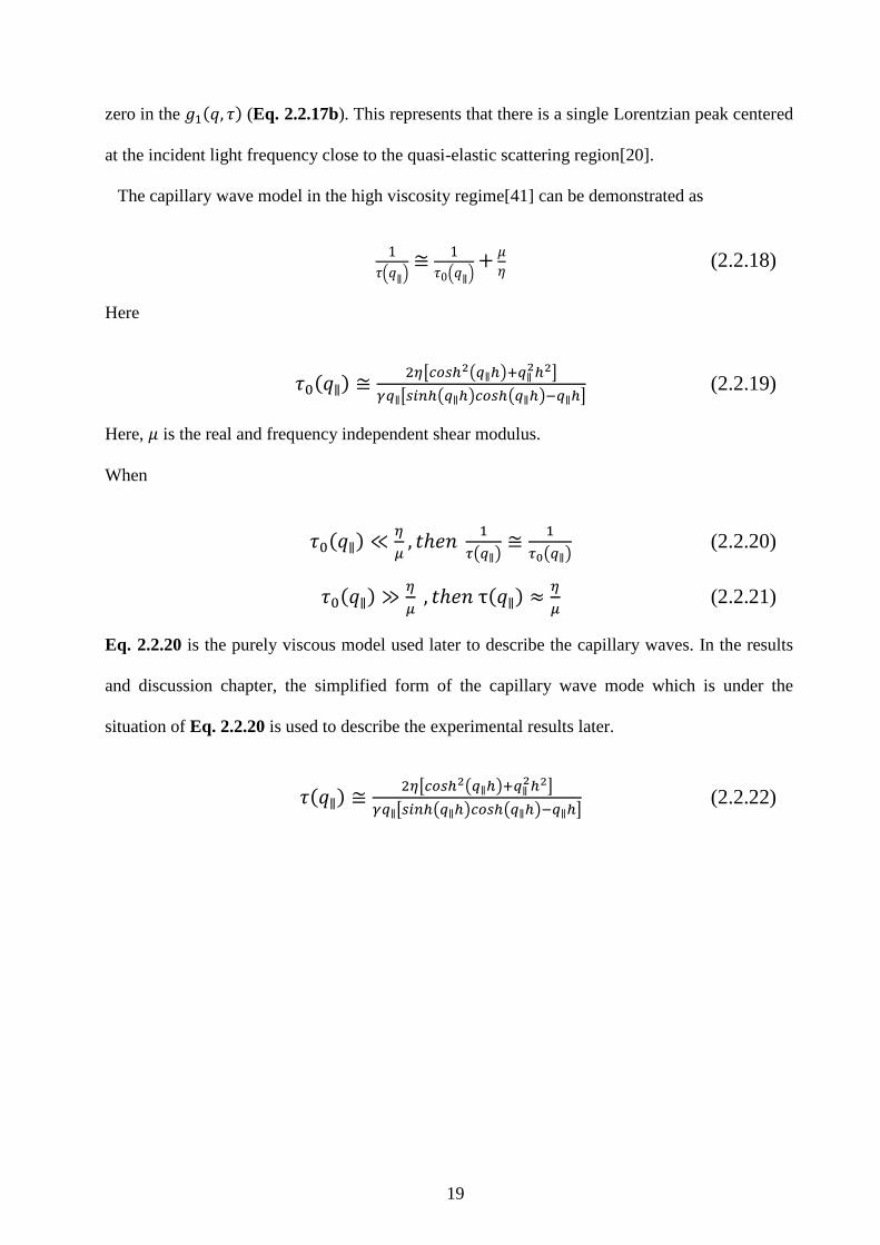
Eq. 2.2.20 is the purely viscous model used later to describe the capillary waves. In the results
and discussion chapter, the simplified form of the capillary wave mode which is under the
situation of Eq. 2.2.20 is used to describe the experimental results later.
𝜏(𝑞∥) ≅2𝜂[𝑐𝑜𝑠ℎ2(𝑞∥ℎ)+𝑞∥
2ℎ2]
𝛾𝑞∥[𝑠𝑖𝑛ℎ(𝑞∥ℎ)𝑐𝑜𝑠ℎ(𝑞∥ℎ)−𝑞∥ℎ] (2.2.22)

20
FIG. 2.2.2 The power spectrum of surface wave in dimensionless units for a nearly ideal liquid
for kh = 0.01, 0.03, 0.1, 0.3, 1, and 3. Dashed line represents kh = 0.03. χ is the dynamic
susceptibility of the vertical surface displacement with respect to an external force acting
vertically on the liquid surface. 𝜔𝑠 is the frequency which referred to the surface wave on an
ideal liquid of infinite depth. k is the wave vector. Reprinted with permission from Journal of
Physics: Condensed Matter, Vol. 10, Josef Jäckle, The spectrum of surface waves on
viscoelastic liquids of arbitrary depth, Page No. 7127. Copyright [1998], IOP Publishing, LTD.
2.3 Surface plasmon polariton
The free electrons in metals can move freely and thus can be thought of as an electron liquid
with a high density of electrons, about 1023
cm-3
. At optical frequencies, the metal’s free
electrons liquid can sustain surface and volume charge-density oscillations, so-called Surface
plasmon polaritons (SPP) which propagate along the surface of the metal[97]. Several
experimental geometries such as Otto and Kretschmann geometries have been employed to
induce the SPP (FIG. 2.3.3). In this thesis, based on the setup of our REDLS, I will describe the
procedure to induce the SPP by using evanescent waves. Further details can be found in the
literature given by Novotny and Hecht (2012)[97], Raether (1988)[98] and Knoll (1998)[99].
When the light impinges from one medium with the refractive index of n1 to another medium
with the refractive index of n2, light will be split into two at the interface, where a part of the
light will be reflected and the other part of the light will be refracted into the medium. If n1 > n2,

21
the impinging light will be totally reflected beyond a specific angle, the critical angle 𝜃𝑐 which
can be determined by Snell’s law.
𝑛1sin 𝜃1 = 𝑛2 sin 𝜃2 (2.3.1)
Here, 𝜃1 is the incident angle and 𝜃2 is the refractive angle when the light impinges from
medium 1 to medium 2. When the light is totally reflected, there is no light refracted into the
medium 2 and the refractive angle 𝜃2 becomes 90°. If we take the interface between a glass
prism and water as example (FIG. 2.3.1a), the critical angle for total reflection based on Snell’s
law is defined as
sin𝜃𝑐 =𝑛𝑑
𝑛𝑝 (2.3.2)
𝑛𝑑 is the refractive index of the dielectric medium, here it is water in Eq. 2.3.2. The refractive
index of the prism is 𝑛𝑝, and 𝜃𝑐 represents the critical angle for total reflection.
When the incident angle is higher than the critical angle 𝜃𝑐 , the incident light is reflected
totally and there is a so-called evanescent wave exited at the interface between two mediums
with different refractive index. In the experiment, the critical angle 𝜃𝑐 can be found by
measuring the reflectivity with increasing incident angle (FIG. 2.3.1b).
22
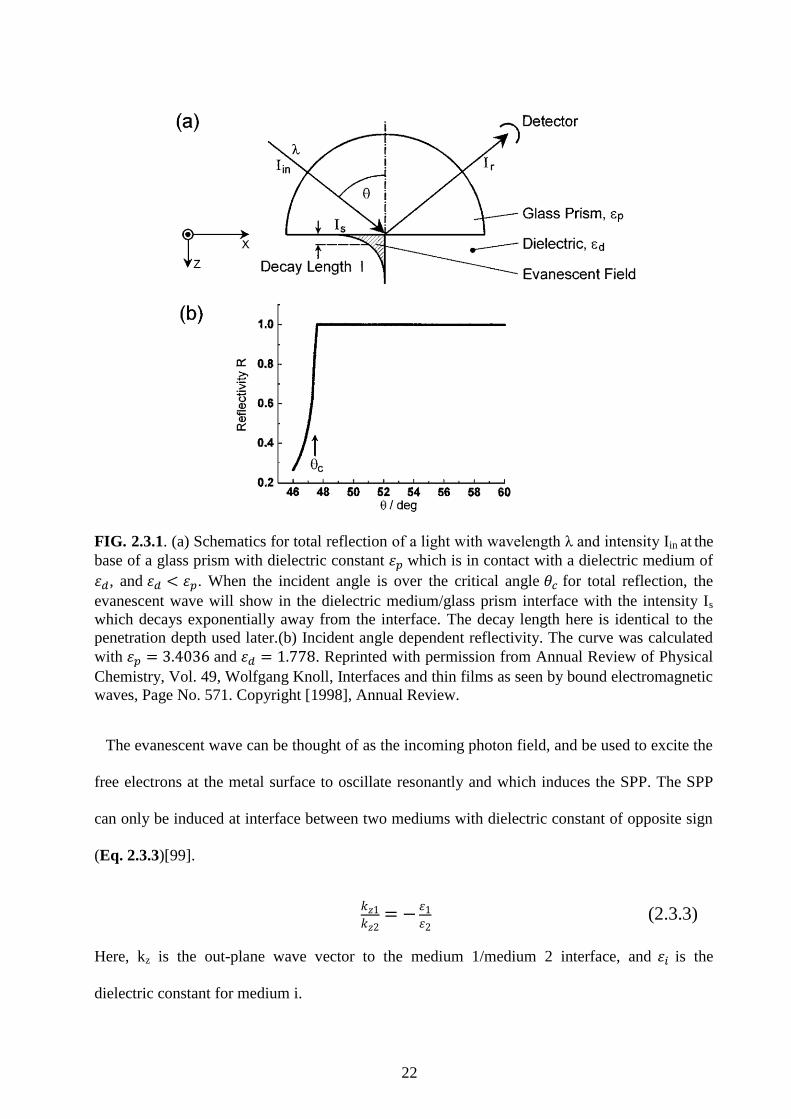
FIG. 2.3.1. (a) Schematics for total reflection of a light with wavelength λ and intensity Iin at the
base of a glass prism with dielectric constant 𝜀𝑝 which is in contact with a dielectric medium of
𝜀𝑑, and 𝜀𝑑 < 𝜀𝑝. When the incident angle is over the critical angle 𝜃𝑐 for total reflection, the
evanescent wave will show in the dielectric medium/glass prism interface with the intensity Is
which decays exponentially away from the interface. The decay length here is identical to the
penetration depth used later.(b) Incident angle dependent reflectivity. The curve was calculated
with 𝜀𝑝 = 3.4036 and 𝜀𝑑 = 1.778. Reprinted with permission from Annual Review of Physical
Chemistry, Vol. 49, Wolfgang Knoll, Interfaces and thin films as seen by bound electromagnetic
waves, Page No. 571. Copyright [1998], Annual Review.
The evanescent wave can be thought of as the incoming photon field, and be used to excite the
free electrons at the metal surface to oscillate resonantly and which induces the SPP. The SPP
can only be induced at interface between two mediums with dielectric constant of opposite sign
(Eq. 2.3.3)[99].
𝑘𝑧1
𝑘𝑧2= −
𝜀1𝜀2
(2.3.3)
Here, kz is the out-plane wave vector to the medium 1/medium 2 interface, and 𝜀𝑖 is the
dielectric constant for medium i.

23
The complex dielectric constant of medium 1 and medium 2, e.g., 𝜀1 = 𝜀1′ + 𝜀1
" and in-plane
complex wave vector 𝑘𝑥 = 𝑘𝑥′ + 𝑘𝑥
" can be applied to describe the properties of SPP. The
medium 1 is assumed as the semi-infinite metal and medium 2 is assumed as air or vacuum
adjacent to medium 1. The dispersion relation for SPP at medium 1/medium 2 interface is[98]
𝑘𝑥 = (𝜀1𝜀2
𝜀1+𝜀2)1/2 𝜔𝑠𝑝
𝑐 (2.3.4)
Here, 𝜔𝑠𝑝 is the angular frequency, c is the light speed in vacuum.
The relation of 𝑘𝑥 and incidence angle θ in the Kretschmann setup[100] which will be
discussed later is shown as[101]
𝑘𝑥 = 𝑛𝑝𝜔𝑠𝑝
𝑐sin𝜃 (2.3.5)
If we assume besides a real 𝜔𝑠𝑝 and 𝜀2 that 𝜀2" < |𝜀1
′ |, the complex in-plane wave vector 𝑘𝑥 is
𝑘𝑥′ =
𝜔𝑠𝑝
𝑐(
𝜀1′𝜀2
𝜀1′+𝜀2
)1/2
(2.3.6)
𝑘𝑥" =
𝜔𝑠𝑝
𝑐(
𝜀1′𝜀2
𝜀1′+𝜀2
)3/2
𝜀1"
2(𝜀1′ )
2 (2.3.7)
The propagation length, 𝐿𝑆𝑃𝑃 of SPP is
𝐿𝑆𝑃𝑃 = (2𝑘𝑥" )
−1 (2.3.8)
The penetration depth, z, for different mediums are
In the medium 2: 𝑧2 =𝜆
2𝜋(𝜀1′+𝜀2
𝜀22 )
1/2
(2.3.9)
In the medium 1: 𝑧1 =𝜆
2𝜋(𝜀1′+𝜀2
𝜀12 )
1/2
(2.3.10)
The SPP is affected by the thickness and dielectric constant of the film which covering the
metal surface where the SPP is excited. This property is used to measure the thickness of

24
polymer thin film by the Surface Plasmon Resonance Spectroscopy (SPR). The shift of 𝑘𝑥 in the
dielectric medium on the top of metal surface is[98]
∆𝑘𝑥(ℎ𝑑) =𝜔𝑠𝑝
𝑐
𝜀𝑑−1
𝜀𝑑(
|𝜀𝑚′ |
|𝜀𝑚′ |−1
)2
|𝜀𝑚′ |+𝜀𝑑
|𝜀𝑚′ |+1
1
√|𝜀𝑚′ |
2𝜋ℎ𝑑
𝜆 (2.3.11)
Here, the hd is the thickness of dielectric medium, εd and εm are the dielectric constants for
dielectric medium and metal, respectively.
In FIG. 2.3.2, the schematics of surface wave propagation and exponential decay of
penetration depth away from the interface is shown.
FIG. 2.3.2. (a) Schematics for the SPP propagation along the metal/dielectric medium interface.
E is the electric field and Hy is the magnetic field in the y-direction. (b) The exponential
dependence of the field Ez is shown. Reprinted by permission from Macmillan Publishers Ltd:
Nature (Vol. 49, William L. Barnes and Alain Dereux, and Thomas W. Ebbesen, Surface
plasmon subwavelength optics, Page No. 826), copyright (2003).
Based on the above discussion, one intuitive way to induce the SPP by evanescent wave is the
Otto-configuration[102] (FIG. 2.3.3a). In the Otto-configuration, the SPP are excited by the tail
of evanescent wave which is induced when the light impinges from glass prism to air over
critical angle 𝜃𝑐. The Otto-configuration is not so practical since the metal surface must be close
to the glass prism within 200 nm and this space is easily affected by the surrounding e.g., dusts.

25
Hence, Kretschmann and Raether[100] introduced another setup for the SPP (FIG. 2.3.3b),
which was also adopted by REDLS. In the configuration proposed by Kretschmann and Raether,
the photons in the glass prism directly couple with the metal to induce the SPP. In the
FIG. 2.3.3b, one side of metal layer is glass prism, and the other is dielectric medium. The
thickness and dielectric constant of the dielectric medium will strongly affect the angle at which
the SPP happens. We make use of these properties to characterize the thickness of polymer thin
film in our study.
The thickness of thin film can be estimated from (Eq. 2.3.5, 2.3.11 and literature[103])
ℎ𝑑 =𝜀𝑎𝑖𝑟𝜆√−𝜀𝑚
′ (𝜀𝑎𝑖𝑟−𝜀𝑚′ )𝜀𝑑
′
2𝜋(𝜀𝑑′ −𝜀𝑎𝑖𝑟)(𝜀𝑑
′ −𝜀𝑚′ )
(𝜀𝑚′ +𝜀𝑎𝑖𝑟
𝜀𝑚′ 𝜀𝑎𝑖𝑟
)2
∆(sinΨ𝑠𝑝𝑝) (2.3.12)
Here, 𝜀𝑎𝑖𝑟 is the dielectric constant of the air, and Ψ𝑠𝑝𝑝 is the resonance angle for the SPP. The
SPP can be found by monitoring the sharp minimum of reflectivity and that angle is the
resonance angle Ψ𝑠𝑝𝑝 (FIG. 2.3.4).
The estimation of film thickness depends on the shift of the resonance angle Ψ𝑠𝑝𝑝, and also
relates to the surrounding optical properties, e.g., the dielectric constant of metal and dielectric
medium. Thus, the refractive index or film thickness cannot be determined independently only
by the shift of the resonance angle Ψ𝑠𝑝𝑝 if not one of the two is known precisely.

26
FIG. 2.3.3. (a) The Otto configuration. 𝜀𝑝, 𝜀𝑑, and 𝜀𝑚 represent the dielectric constant of glass
prism, dielectric medium, and metal, respectively. (b) Attenuated total internal reflection (ATR)
for the SPP excitation in the Kretschmann configuration. Reprinted with permission from
Annual Review of Physical Chemistry, Vol. 49, Wolfgang Knoll, Interfaces and thin films as
seen by bound electromagnetic waves, Page No. 578. Copyright [1998], Annual Review.
27
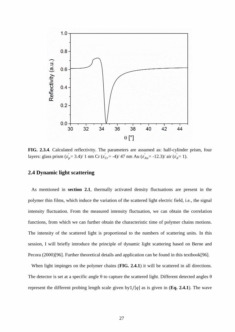
FIG. 2.3.4. Calculated reflectivity. The parameters are assumed as: half-cylinder prism, four
layers: glass prism (𝜀𝑝′ = 3.4)/ 1 nm Cr (𝜀𝐶𝑟
′ = -4)/ 47 nm Au (𝜀𝐴𝑢′ = -12.3)/ air (𝜀𝑑
′ = 1).
2.4 Dynamic light scattering
As mentioned in section 2.1, thermally activated density fluctuations are present in the
polymer thin films, which induce the variation of the scattered light electric field, i.e., the signal
intensity fluctuation. From the measured intensity fluctuation, we can obtain the correlation
functions, from which we can further obtain the characteristic time of polymer chains motions.
The intensity of the scattered light is proportional to the numbers of scattering units. In this
session, I will briefly introduce the principle of dynamic light scattering based on Berne and
Pecora (2000)[96]. Further theoretical details and application can be found in this textbook[96].
When light impinges on the polymer chains (FIG. 2.4.1) it will be scattered in all directions.
The detector is set at a specific angle θ to capture the scattered light. Different detected angles θ
represent the different probing length scale given by1/|𝑞| as is given in (Eq. 2.4.1). The wave

28
vectors of the evanescent (incident) and the scattered electric field are defined as �⃑� 𝑖 and �⃑� 𝑠 ,
respectively (FIG. 2.4.1). Thus, the scattering wave vector is defined as q :
𝑞 ≔ |�⃗�| = |�⃑� 𝑖 − �⃑� 𝑠| =4𝜋𝑛
𝜆sin (
𝜃
2) (2.4.1)
Here, λ is the wavelength of incident light and n is the refractive index of the sample.
The scattered light received by the detector at a given time is the superposition of radiated
electric fields from polymer molecules in the scattering volume. The superposition of electric
fields forming a speckle field will fluctuate with time since the dynamics of molecules is
affected by the thermal fluctuation. In order to exact the characteristic time of the polymer
dynamics, the time-dependent correlation function is applied to analyze the time-dependent
fluctuating electric filed.
The output of the detector represents the intensity of scattered electric field, and their relation
is 𝐼(𝑞, 𝑡) ∝ |𝐸(𝑞, 𝑡)|2 . Here, 𝐼(𝑞, 𝑡) and |𝐸(𝑞, 𝑡)| are defined as the intensity and scattered
electric field at a specific scattering wave vector q and time t. The intensity-intensity time
autocorrelation function is shown as
⟨𝐼(𝑞, 𝑡0)𝐼(𝑞, 𝑡0 + 𝑡)⟩ = 𝐶𝑒𝑓𝑓𝑖𝑐𝑖𝑒𝑛𝑐𝑦⟨|𝐸(𝑞, 𝑡0)|2|𝐸(𝑞, 𝑡0 + 𝑡)|2⟩ (2.4.2a)
Here, the Cefficiency is a proportionality constant related to the efficiency of the detector.
In the so called homodyne method, only the scattered light from the polymer molecules
contributes to the intensity signal. Thus, ⟨𝐼(𝑞, 𝑡0)𝐼(𝑞, 𝑡0 + 𝑡)⟩ is proportional to the homodyne
correlation function 𝑔2(𝑞, 𝑡). The Eq. 2.4.2a can be recast as
𝑔2(𝑞, 𝑡) ≡ ⟨|𝐸(𝑞, 𝑡0)|2|𝐸(𝑞, 𝑡0 + 𝑡)|2⟩ (2.4.2b)
If the intensity signal is a mixed contribution from a local oscillator (unscattered, direct or
elastic light), this technique is called heterodyne detection. The heterodyne method enhances the
signal intensity and raises the S/N ratio. In the heterodyne method, the local oscillator and the
scattered light are mixed, so the autocorrelation function Eq. 2.4.2a is modified to

29
⟨𝐼(𝑞, 𝑡0)𝐼(𝑞, 𝑡0 + 𝑡)⟩ = 𝐶𝑒𝑓𝑓𝑖𝑐𝑖𝑒𝑛𝑐𝑦⟨|𝐸𝑙𝑜𝑐(𝑞, 𝑡0) + 𝐸(𝑞, 𝑡0)|2|𝐸𝑙𝑜𝑐(𝑞, 𝑡0 + 𝑡) +
𝐸(𝑞, 𝑡0 + 𝑡)|2⟩
(2.4.2c)
Here, 𝐸𝑙𝑜𝑐(𝑞, t) is defined as the electric field of the local oscillator.
Based on the following approximations we obtain the field autocorrelation function g1(t)
directly:
(1) |𝐸𝑟𝑒𝑓(𝑞, t)| ≫ |𝐸(𝑞, t)|
(2) The fluctuation of the electric field from the reference light is negligible.
(3) The electric fields of scattered light and reference light (local oscillator) are statistically
independent
The homodyne correlation function 𝑔2(𝑞, 𝑡) and heterodyne correlation function 𝑔1(𝑞, 𝑡) are
connected via Siegert relation
𝑔2(𝑞, 𝑡) = 𝐶𝑏𝑎𝑠𝑒[1 + 𝑓|𝑔1(𝑞, 𝑡)|2] (2.4.2d)
Here, Cbase is the baseline and f is the correction factor for the instrument, both of them are
constants.
FIG. 2.4.1. Schematics for dynamic light scattering. Here, the wave vector of incident light is
defined as �⃑� 𝑖, and of the scattered light is defined as �⃑� 𝑠. The angle between �⃑� 𝑖 and �⃑� 𝑠 is defined
as θ.

30
Chapter 3
Materials and Experimental Methods
In this chapter, the sample preparation and the main experimental method, REDLS, will be
introduced. Different methods of data analysis will be compared. The estimation of error for the
experimental data of the custom-made REDLS will be also discussed.
3.1 Sample preparation
Our samples consist of polymer thin films and metal thin films which are supported by the
glass substrate. The substrates used here are highly polished glass slides (Hellma, N-LaSF9).
First a 1 nm Cr-layer was deposited by thermal evaporation onto the substrate to make sure that
the following Au-layer is attached well. Subsequently a layer of 47 nm of Au was deposited in
order to induce the SPP to be the light source. Then, the polymer thin films were spin-coated on
the top of Au layer. The polymers were dissolved in toluene (HPLC-grade, Sigma Aldrich).
Between 0.5 and 2 wt% solutions were spin-coated onto the Au coated glass substrate at 1000-
5000 rpm for 5 to 10 minutes to prepare and dry the films. The 45 nm thin film usually could be
obtained from 1 wt% solution at the speed of 1000 rpm. Since the thickness of thin films made
by spin-coating are easily affected by the surroundings, the exact spinning-speed and the
concentration of solution has to be modified each time one prepares films. Three different
samples are used in this thesis: (1) PB thin films, (2) PS/PN bilayers consisting of PS thin films
on the substrates covered by a thin film of PN, (3) PS thin films anchored to Au surface by PS
polymers with a thiol group as end group. All the solutions used below were filtered through 0.2
μm PTFE filter (Rotilabo-syringe filter, not sterile, Carl Roth GmbH+Co. KG). All the thin
films were prepared using glass syringes and stainless steel needles to avoid the contamination

31
by lubrication oil which is commonly used inside the plastic syringes and needles for medical
application. Before preparing the polymer solution, all the glass syringes and stainless steel
needles were rinsed and cleaned thoroughly by the solvent.
3.1.1 Polybutadiene (PB)
Polybutadiene (45% 1,4-cis-, 45% 1,4-trans-, 10% 1,2-vinyl) of two different molecular
weights (as obtained by GPC), synthesized at Max Planck Institute for Polymer Research (MPIP)
by anionic polymerization, was used. One, PB50, has molecular weight Mw= 50 kg/mol,
Mw/Mn=1.08, and Tg = 172 K, the other, PB267, Mw= 267 kg/mol, Mw/Mn=1.10, and Tg = 175 K.
A refractive index of n = 1.52 for the PB[104,105] was used subsequently in our analysis. Both
polymers are well above the entanglement molecular weight and should show similar relaxation
behavior. The viscosity of PB267 should be slightly higher due to the slightly higher Tg. These
polymers, however, have a different radius of gyration; Rg of 8.5 nm for PB50 and 19.5 nm for
PB267[106]
chosen by us to test theoretical predictions about the dependence of confinement on
dynamics on Rg or a multiple of it.
The polystyrene film was spin-coated on the Au substrate for 5 minutes. After spin-coating,
samples were annealed in vacuum at room temperature (Tg+125K) for 12 hrs. This annealing
removes satisfactorily the solvent from the films. No additional diffusion process of solvent in
the films was detected in our experiments. The thickness of the films was checked by SPR
(Eq. 2.3.12).
3.1.2 Polystyrene/ polynorbornene (PS/ PN) bilayers
The PS/PN bilayer is the PS thin film capped by the PN layer. Later in the results and
discussions, the sample of PS capped by PN layer is presented like
PS+thicknessPS+PN+thicknessPN. For example, the PS45PN20 means PS 45nm is capped by PN
layer 20 nm.

32
Polystyrene used was synthesized at MPIP by anionic polymerization. The molecular weight
(Mw) is 1821 g/mole (as obtained by GPC), Mw/Mn = 1.08, and Tg = 326 K. A refractive index
of n = 1.59 for the PS[107] was used subsequently in our analysis.
The polystyrene was spin-coated onto the Au coated glass substrate for 10 minutes. After spin-
coating, samples were annealed in vacuum. The samples were annealed with the following steps.
First, the samples were annealed at 338K for 12hrs. Then, the temperature was increased to
348K for 12hrs. Finally the sample temperature was kept at 353K over 48hrs. This annealing
removes satisfactorily the solvent from the films. No additional diffusion process of solvent in
the films was detected in our experiments.
The norbornene monomer (Sigma-Aldrich, 99% purity, bp. 338K, vapor pressure 52mbar at
298K) is used to ignite a norbornene-plasma which then polymerizes on top of the polystyrene
film forming a crosslinked PN layer. A cylindrical Pyrex plasma reactor was used, the details
about the reactor and plasma-polymerized process are described elsewhere[108-110]. The
pressure of the norbornene gas was controlled to be 0.05 mbar. A pulsed mode of plasma which
is generated by setting ton = 20 ms and toff = 50 ms of plasma was adopted with an input power
of radiofrequency at 50W. The thickness of PN layer was adjusted by the time of plasma reactor
is switched on. The deposition rate was estimated of ~10 nm/min. Finally, the thickness of the
films was checked by SPR.
3.1.3 PS thin film anchored to Au surface by thiol group
PS and the thiol terminated PS-SH used were synthesized at MPIP by using anionic
polymerization. A refractive index of n = 1.59 for the PS[107] was used subsequently in our
analysis.
The Mw of PS is 2695 g/mol (as obtained by GPC), Mw / Mn=1.06, and Tg = 326 K. The Mw of
the PS which was modified by a thiol (-SH) group at the end is 3000 g/mol, Mw / Mn=1.2. The
PS-SH was dissolved in toluene (HPLC-grade, Sigma Aldrich) at the concentration of 1mM.

33
Then the prepared gold thin film supported by the glass substrate was immersed in the 1mM PS-
SH /toluene solution for 72hrs. After 72hrs, the substrate with the now covalently attached PS-
SH was rinsed by the toluene solvent 10 times to remove the unbound PS-SH.
The PS of 2695 g/mole was spin-coated onto the Au coated glass substrate for 5 minutes. After
spin-coating, samples were annealed in vacuum. The annealing temperature was processed in
three stages. In the first stage, the samples were annealed at 338K for 12hrs. Second, the
temperature was increased up to 348K for 12hrs, and then maintained the temperature at 353K
over 48hrs. The above annealing process removes satisfactorily the solvent from the films. No
additional diffusion process of solvent in the films was detected in our experiments.
The thickness of the films was characterized by SPR. Here, all the samples are named by the
PS-SH/PS with the PS film thickness. For example, the PS-SH/PS85 represents the Au layer
modified by PS-SH, and there is a layer of 85 nm of PS on top.
TABLE 3.1.1 The polymers we used to prepare samples in this thesis. P.D.I. polydispersity
index, n refractive index
Abbrev. Polymer Mw (g/mole) P.D.I. Tg n
PB50 Polybutadiene 50000 1.08 172K 1.52
PB276 Polybutadiene 276000 1.10 175K 1.52
PS Polystyrene 1820 1.08 326K 1.59
PS Polystyrene 2695 1.06 326K 1.59
PS-SH Polystyrene modified
by thiol end group
3000 1.20 283K 1.59
P.D.I. is the polydispersity and defined by Mw/Mn.
3.2 Resonance enhanced dynamic light scattering
REDLS (FIG. 3.2.1)[55,56] is a non-invasive, marker free technique to probe the dynamics of
polymer thin films supported on a noble metal, in our case Au, to excite the SPP at the
resonance angle ΨSPP. The SPP is adopted to be the light source with penetration depth ξ = 200

34
nm. The light is scattered by the polymer thin film on the top of Au layer and collected by the
DLS at an angle .
First, we have to attach our sample, the substrate with the film on top to the top of a half-
cylinder prism . There are two reasons to use a half-cylinder prism here. One is that we can
excite the SPP at a lower resonance angle ΨSPP when we measure the film with h > 60 nm. The
other is, geometrically the SPP is always excited at the center of Au substrate which coincides
with center of the goniometer in the REDLS (FIG. 3.2.2) at any resonance angle ΨSPP. This is
not the case for angular prism where due to refraction the angle can shift substantially. Therefor
it is easier in DLS to align the scattering light spot in/on the polymer thin film. We use PS of Mw:
400 g/mole to be the matching oil between the sample and the prism. The refractive index of
matching oil should be as close as possible to the one of the prism, and does prevent internal
reflection between the substrate and the prism which can interfere with the SPR measurement.
When using PS of refractive index of 1.59 here to match the LaSFN9 prism and glass substrate
with refractive index of both is 1.81 at λ= 632.8 nm, internal reflection and interference happen
at angles over 55°; because of the half-cylinder prism we do not have to go to such high angles
and therefor the interference is not hindering the experiment. The reason we choose PS to be the
matching oil is because we will perform temperature dependent experiments and the matching
oil is required to be thermally stable even at high temperature (over 373K) which is not the case
for the commercially available matching oils which will fit better for the index matching.
When the light of a He-Ne laser (wave length λ=632 nm) impinges at the resonance angle ΨSPP
on the sample, the evanescent part of the SPP is excited on the Au surface to be the light source
in our dynamic light scattering experiment. In the experiments, the SPP is excited at the angle of
the minimal reflectivity (FIG. 2.3.4) ΨSP. The sample is covered by a hemispheric quartz sample
holder with N2(g) inside it to prevent the sample from oxidizing during measurement.
The light induced by the SPP will be scattered by the polymer thin film on the top of Au-layer
since there are density fluctuations in and on the film. The REDLS is a heterodyne DLS setup.

35
This means the scattered light is mixed with light from a local oscillator formed by elastic,
scattered light induced by the roughness of the gold film. One thing one has to make sure of is
the amplitude of the local oscillator has to be much greater than the scattered light. According to
the literatures[55,57,111], the intensity of signal contributed from the local oscillator is 1000
times or higher than the scattered light by choosing the proper surface plasmon radiation to
ensure fully heterodyne DLS. The scattered light is collected at varying scattering angles θ (or
wave vector q) by two photomultipliers (MP-973(6606-P-079)-Perkin Elmer) to obtain the
pseudo cross-correlation function by using an ALV7004 fast multiple tau digital correlator
(ALV, Germany). The pseudo cross-correlation is adopted to eliminate undesired signals[112].
The incoming signal is split into two to two photon detectors and their outputs into a correlator.
The real data of intensity fluctuation and g1 correlation function is shown (FIG. 3.2.3). The
scattering wave vector q is defined as Eq. 2.4.1.
The REDLS setup sits on an anti-vibration table and is housed in a black housing to prevent
and minimize interference from the surroundings. The anti-vibration system (AVI-350/LP,
Table Stable) we use is a piezo-coil damping mechanism designed for vibration frequency from
1-200Hz with a damping of better than 35dB. The high frequency part of the vibration spectrum
is passively damped by using an aluminum breadboard.
The capillary wave of polymer thin films is sensitive to temperature fluctuation. Temperature
fluctuation induced by the environment can contribute to the signal and lead to spurious
correlated signals. In order to prevent this we always used a heater to control the temperature by
a control loop feedback mechanism, i.e., proportional-integral-derivative (PID) controller. In the
PID controller, we set different values of 1, 0.1, and 0.01 for the Integral parameter in the PID to
test if the feedback loop of the heater causes systematic errors producing correlated signals by
e.g. systematically expanding/shrinking parts. At the integral value = 1, the signal we receive is
influenced by the oscillation of temperature feedback loop. In the integral vales = 0.1 and 0.01,
there is no influence to the signal. The temperature of the film is measured with a PT100 (#9 in

36
FIG. 3.2.2) pressed onto the film well outside of the scattering volume. The thermo sensor for
the heating control is in the base of the prism holder (#8 in FIG. 3.2.2) to ensure quick reaction
on temperature changes.
The scattering angle θ is an off-plane angle, and q|| is the component of the wave vector q
parallel to the substrate plane. Because the capillary wave propagates along the surface of the
film, q has to be replaced by q|| to describe the dynamics properly[7]. q|| and 𝑞⊥ are defined as
q∥: = |q
∥⃑⃑ ⃑|=|q⃑ |∙ cos (
180°-θ
2); q
⊥: = |q
⊥⃑⃑⃑⃑ |=|q⃑ |∙ sin (
180°-θ
2) (3.2.1)
In REDLS one measures fully heterodyne correlation functions due to the mixing of elastic
light from the Au surface[111] as local oscillator and the scattered light[55,56]. The related data
analysis will be shown in the section 3.3.

37
FIG. 3.2.1. Schematics of the REDLS setup. The LASER beam impinges at the resonance angle
ΨSPP on the gold-glass boundary to excite the SPP in the gold layer with an evanescent field with
a penetration depth ξ of 200 nm into the dielectric above. The polymer thin film is on the Au
surface. The scattered light from the polymer layer is collected by the DLS detector system at a
scattering angle . Polarized and depolarized light scattering is feasible via the build in
polarizers to select the according combination of polarized light. The REDLS setup is adapted
from Vianna’s Ph.D. works.[57]

38
FIG. 3.2.2. REDLS setup: (1) He-Ne LASER λ=632.8 nm (2) photo-diode detector for the SPP
(3) sample holder (4) goniometer from Optrel (Multiskop) (5) N2(g) connection to sample holder
(6) holder for optical fiber which connects to the DLS detector (7) heater (8) thermo-sensor
(PT100) for heating control (9) thermo-sensor (PT100) for monitoring the sample temperature
(10) quartz holder to keep the sample holder under the N2(g) surrounding. The inset is the larger
figure for the sample holder.
FIG. 3.2.3. Typical experimental data: (a) Time-dependent intensity fluctuation for PS thin film
of 45 nm thick at 366K and q = 0.78x10⁻²
[nm-1
]. (b) Normalized heterodyne autocorrelation
function in VV polarization which is calculated from intensity fluctuation (a) by the correlator
automatically.

39
3.3 Data analysis
Despite the low polydispersity of our samples (see TABLE 3.1.1), there is an inevitable
molecular weight distribution. This remaining polydispersity as well as hydrodynamic
interactions of the solid substrate and the liquid-gas interphase on the dynamics lead to a
distribution of relaxation times or rates. This distribution is expected to have a different form
compared to the distribution in diffusion experiments in bulk solution following e.g. the
distribution in sizes of particles. Thus e.g. fitting by the Cumulant[113] method is not justified
in our case. Hence, we fitted the heterodyne auto-correlation functions by the empirical
Kohlrausch-Williams-Watts equation (KWW) - the so-called stretched exponential decay.
C(q,t)=a exp {- (t
τ)β
} , Γ=1
τ; 0<β≤1 (3.3.1)
Here, the C(q, t) is our measured heterodyne auto-correlation function, a is the amplitude of
the decay, τ is the relaxation time, and β is the stretching parameter describing the distribution of
relaxation times. The physical relevant parameter is the mean relaxation rate <> or the mean
inverse relaxation time[114]
⟨Γ⟩ = ⟨1
τ⟩ =
β
τ ∙
1
𝐺𝑎𝑚𝑚𝑎 [1/β] (3.3.2)
with Gamma the gamma function. For simplicity in the following we denote <> as .
The comparison and discussion of different fitting methods are processed in the following:
In scattering theory, the diffusional motions of an ideal system of monodisperse particles are
described by:
𝑔1(𝑞, 𝑡) = 𝑒𝑥𝑝(−𝛤𝑡), Г = 1/𝜏 (3.3.3)
the heterodyne correlation function. Here, Г is the relaxation rate, the relaxation or
characteristic time of this motion.

40
Due to the aforementioned reasons the relaxation process describing a motion has not a single
exponential shape as in Eq. 3.3.3. Moreover, the samples do not show only one mode of motion,
but combine different kind of motions at the same probing time and length; e.g., rod-like
particles show translation and rotation.
Several methods have been developed to describe the decay function. Here, three widely-used
methods are compared: Cumulant expansion [113], CONTIN [115,116] and Kohlrausch-
Williams-Watts (KWW)[117,118]. We compare different distributions of relaxation time to
examine the applicability of the above approaches.
3.3.1 Cumulant expansion
The Cumulant expansion is a method to expand the heterodyne correlation function by power
series. For the multi-exponential decay, the Eq. 3.3.3 is rewritten as:
𝑔1(𝑞, 𝑡) = ∫ 𝐺(𝛤)𝑒𝑥𝑝(−𝛤𝑡)𝑑𝛤∞
0 (3.3.4)
with
∫ 𝐺(𝛤)𝑑𝛤 = 1∞
0 (3.3.5)
Here, 𝐺(Γ) is the distribution function of the relaxation rates, and the distribution from the
mean is a Gaussian curve. The mean value is defined as
𝑔1(𝑞, 𝑡) = 𝑒𝑥𝑝(−𝛤𝑡)𝑒𝑥𝑝(−(𝛤 − ⟨𝛤⟩)𝑡) (3.3.6)
Expanding Eq. 3.3.4 by power series
𝑔1(𝑞, 𝑡) = ∫ 𝐺(𝛤)∞
0𝑒𝑥𝑝(−⟨𝛤⟩𝑡) [1 − (𝛤 − ⟨𝛤⟩)𝑡 +
(𝛤−⟨𝛤⟩)2
2!𝑡 − ⋯ ]𝑑𝛤
(3.3.7)
𝑔1(𝑞, 𝑡) = 𝑒𝑥𝑝(−⟨𝛤⟩𝑡) (1 +𝑘2
2
2!𝑡2 − ⋯) (3.3.8)
𝑙𝑛 𝑔1(𝑞, 𝑡) = − ⟨𝛤⟩𝑡 +𝑘2
2
2𝑡2 − ⋯ (3.3.9)

41
Here, 𝑘2 = ∫ 𝐺(Γ)∞
0(Γ − ⟨Γ⟩)2𝑑Γ
The method of Cumulants assumes the distribution of relaxation time to be narrow. In order to
fit heterodyne correlation functions with a broad distribution of relaxation time, the method of
CONTIN was developed to get a better estimate.
3.3.2 CONTIN
CONTIN[115,116] belongs to the class of constrained regularized methods of which it is the
most used in data analysis of DLS data.
The distribution function 𝐺(Γ) can be transformed to a sum of single-exponential decay
functions by Laplace transformation.
ℒ[𝐺(𝛤)] = ∫ 𝐺(𝛤)∞
0𝑒𝑥𝑝(−⟨𝛤⟩𝑡) = 𝑔1(𝑞, 𝑡) (3.3.10)
We have to find the corresponding distribution function by inverse Laplace transformation
from 𝑔1(𝑞, 𝑡).
𝐺(𝛤) = ℒ−1[𝑔1(𝑞, 𝑡)] (3.3.11)
This is a so called ill-posed problem since there are infinite solutions existing to satisfy
Eq. 3.3.11 within small experimental error. Hence, in the method of CONTIN, some constraints
have to be used. There are three strategies to achieve this goal[119]:
Limiting of the extent of information being recovered: The number of components of the
distribution function is limited.
Incorporation of a prior knowledge: the non-negativity constraint, assume a specific
analytical form and a certain more general feature of the distribution function.
Parsimony or regularization: the simplest of all possible solutions compatible with the
data is taken.

42
3.3.3 Kohlrausch-Williams-Watts function
The fitting function used in this study is named Kohlrausch-Williams-Watts (KWW) function
or stretched exponential function. This is a straightforward fitting method to describe the
distribution of relaxation time problem by tuning the power law.
𝑔1(𝑞, 𝑡) = 𝑎 𝑒𝑥𝑝 {−(𝑡
𝜏)𝛽
} ; 𝛽 = ]0,1] (3.3.12)
Here, a is the amplitude of the decay β is the stretching parameter. In the dynamic light
scattering, the stretching parameter β is a measure for the width of the distribution of relaxation
times.
The physical relevant relaxation parameter is the mean relaxation time or rate:
<1/τ>=β<1/τ>/Gamma[1/β] with Gamma the gamma function.
FIG. 3.3.1. Simulation of KWW function, Eq. 3.3.12, with different stretching parameters β
from 0.5 to 1. The <Γ> is set to 100s-1
. The relaxation rate Γ of each β is defined by the relation
<1/τ>=β<1/τ>/Gamma[1/β].
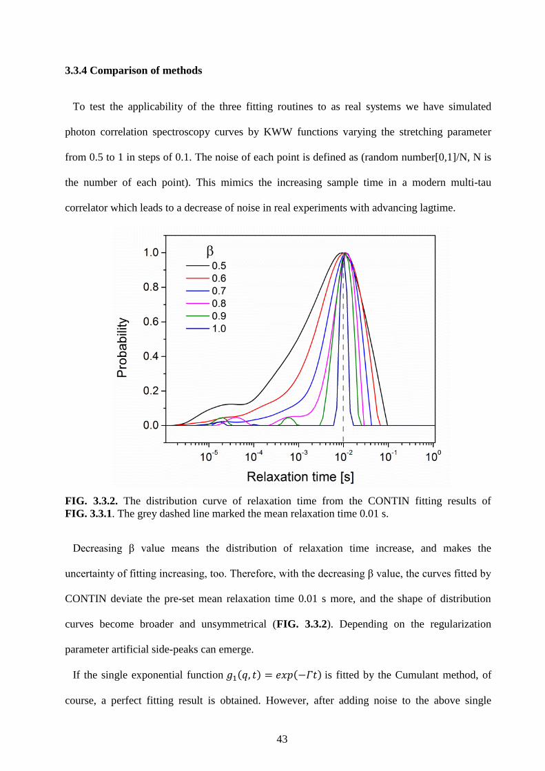
43
3.3.4 Comparison of methods
To test the applicability of the three fitting routines to as real systems we have simulated
photon correlation spectroscopy curves by KWW functions varying the stretching parameter
from 0.5 to 1 in steps of 0.1. The noise of each point is defined as (random number[0,1]/N, N is
the number of each point). This mimics the increasing sample time in a modern multi-tau
correlator which leads to a decrease of noise in real experiments with advancing lagtime.
FIG. 3.3.2. The distribution curve of relaxation time from the CONTIN fitting results of
FIG. 3.3.1. The grey dashed line marked the mean relaxation time 0.01 s.
Decreasing β value means the distribution of relaxation time increase, and makes the
uncertainty of fitting increasing, too. Therefore, with the decreasing β value, the curves fitted by
CONTIN deviate the pre-set mean relaxation time 0.01 s more, and the shape of distribution
curves become broader and unsymmetrical (FIG. 3.3.2). Depending on the regularization
parameter artificial side-peaks can emerge.
If the single exponential function 𝑔1(𝑞, 𝑡) = 𝑒𝑥𝑝(−𝛤𝑡) is fitted by the Cumulant method, of
course, a perfect fitting result is obtained. However, after adding noise to the above single

44
exponential function, but β value remains at one, a poorer fitting result is obtained (FIG. 3.3.3a).
With decreasing β value, the correlation functions are hardly fitted by the Cumulants well
(FIG. 3.3.3b). Actually, besides the first term in Eq. 3.3.9, the remained parts do not give a
good estimate of correlation functions.
FIG. 3.3.3. (a) Comparison of the single exponential decay function g1(q, t) = exp(−Γt) with
noise () and without noise (). (b) Comparison of Cumulants fitting results of FIG. 3.3.1. All
of the solid lines are fitted by the Eq. 3.3.9 to the quadratic term.
With increasing β value, the deviating relaxation times of Cumulants method converge to the
pre-set value (FIG. 3.3.4a). When different fitting methods are compared at β=0.7 (FIG. 3.3.4b),
the results of KWW and CONTIN almost coincide. However, the result of Cumulants is not as
good as CONTIN, but still in the reasonable error range (within the central part of peak).

45
FIG. 3.3.4. (a) The relaxation time of heterodyne correlation functions in FIG. 3.3.1 at the
different β value from KWW(), CONTIN(), and Cumulants(). (b) The distribution curve
of relaxation time in the β=0.7. The different types of lines mark the relaxation time from
methods: KWW (dash-dotted line), CONTIN (dash), and Cumulants (dot). Here, all the
relaxation time of KWW is the mean relaxation time set to 0.01 s.
Comparing these three fitting methods, the KWW function is the method to describe the
heterodyne correlation function. And it also shows the fitting results are better than CONTIN
and Cumulants especially at smaller β value. Hence, it can be applied to solve the distribution of
relaxation time problem, describe the correlation function well, and get a good estimate of
relaxation times.
3.4 Experimental errors
The viscosities are fitted by the simplified capillary wave model[7]. Hence, the uncertainties
are probably from several factors: surface tension, relaxation time, q||, and the film thickness.

46
The surface tension and relaxation time are affected by temperature. The error in surface tension
and relaxation time from the error in temperature can be estimated by the influence on d/dT=-
0.065 (mN/m K) and VFT law [120-122]. The q|| is affected by measuring the angle decided by
the precision of the machine. The errors induced by the uncertainties of surface tension,
relaxation time, and q|| are less than 4%. Compared to the uncertainties induced from thickness,
the effects from the surface tension, relaxation time and q|| errors are much smaller and can be
neglected.
The thickness of our films is measured by Surface Plasmon Resonance Spectroscopy (SPR).
The error of thickness characterized by SPR is usually much less than 1 nm if the film is
attached in situ in the SPR experiment. In our case in order to change samples easily, we have to
spin-coat the thin film on glass substrates and use matching oil between glass substrate and
prism. However, it is impossible to get exactly the same thickness of matching oil every time.
This layer also affects the fit results for the thickness of thin films. The worst case leads to an
error of film thickness of ±2 nm. Therefore the largest error of viscosity in the thinner films is
about 23% (as shown as error bar in PB 50, 23 nm, (FIG 4.1.6b). The error bar for viscosity is,
due to the logarithmic scale smaller than the symbol size.

47
Chapter 4
Results and Discussion
In Sulivan D.B. Vianna’s PhD thesis[57], the capillary waves of polystyrene (PS) thin films
were measured above but close to Tg. In cooperation with the theory group of Prof. Dr. Kurt
Kremer at the Max Planck Institute for Polymer Research and the group of Prof. Dr. Klaus
Rätzke at the University of Kiel, the density and free volume voids of PS thin film at an Au
interface were studied[35] by multiscale molecular simulation and positron annihilation lifetime
spectroscopy (PALS). In the experimental part, PALS, shows a higher density of polymer chains
at the Au/PS interface and smaller free volume voids in the thin film compared to the bulk.
These experimental results are in agreement with the simulation results from the multiscale
molecular dynamics simulations where the higher density of polymer chains is found to be close
to the Au/PS interface.
Based on this study, we measure polymer thin films in different elastic modulus and are
changing the confinement imposed on the thin films to observe how e.g. the substrate affects the
capillary wave dynamics. One approach is to use PB thin films which are a liquid at our
measuring temperature which is above Tg + 125K. Compared to the PS, the PB thin film is a
suitable low viscosity sample to test the capillary wave model in different polymer film
thickness. In a second approach, the capillary wave of PS thin film is suppressed by a glassy
capping layer to answer if there are other motions contributing to the thin film dynamics. The
third approach is to test the influence of a more or less immobilized layer at the substrate
interface, the PS is anchored to the substrate by thiol group. The dynamics of capillary waves
can be tuned via modifying the interaction at the substrate/polymer interface and prove the
existence of several modes of motions at the polymer/air interface and in the polymer.

48
4.1 Capillary wave dynamics of thin liquid PB films
The confinement on different length scales can be affected e.g. by type of substrate, modulus
of thin film, and temperature. Thin films of PS close to Tg where studied by Vianna[57]. Hence,
one of the polymer materials studied in this thesis, PB, is a polymer which is close to the
behavior of a Newtonian fluid since it is being used for experiments at very high temperatures
compared to Tg. On the other hand it is in the entanglement region of high Mw and one should be
able to observe how long-range motions of polymer chains are suppressed by a less mobile
layer[46,123] at the interface to the solid substrate. We measured the polybutadiene (PB) at
298K (i.e. Tg + 125K), where the thin films are liquid. To be in the same range PS will have to
be heated to 450K and more to be close to a Newtonian liquid. At these high temperatures these
PS films are not stable. The molecular weights of PB we studied are beyond 50 kg/mol
corresponding to the highly entangled region (entanglement Mw: 1.85 kg/mole)[124].
This also avoided thin film dewetting and kept the films mechanically stable during
measurement. Here, we did not do temperature dependent measurement. The reason is, the
purpose of this study is to observe the confinement effects at the low modulus and high
temperature region, and start from a single measuring temperature. Most of the results we
observe can be described by capillary wave models[2,20], but we find that the viscosity of the
PB thin films is sensitive to the film thickness. We account for the mechanism of our findings
by using a three layer model.
The following results and discussion of section 4.1 are adapted and partially reprinted with
permission from Journal of Chemical Physics, Vol. 141, Fan-Yen Lin and Werner Steffen,
Capillary wave dynamics of thin liquid polymer films. Copyright [2014], AIP Publishing LLC.

49
4.1.1 Results and discussion
Film stability
A dewetting during the experiment shows up as a drastic change in incident intensity in the
REDLS experiment due to the change in local refractive index. In cases we observed this, we
discarded the measurements.
Here, the AFM images (FIG. 4.1.1 and 4.1.2) are obtained after the REDLS measurement.
There is no dewetting pattern observed in the topography images of different scale at thickness
25 nm and 75 nm for PB50 (FIG. 4.1.1a, c and 4.1.2a, c). The roughness (rms) of PB50 at
thickness 25 nm and 75 nm are lower than 1nm for the range below 1μm1μm. This roughness
may be induced by the dynamic heterogeneities in a thin liquid-like layer at the glassy polymer
surface as reported[125]. All the samples were measured in contact mode at 298K under 1 atm
in air (Dimension 3100, Digital Instruments).
Most experiments conducted in the past on polymers in thin films were done in a low
temperature regime, i.e. above and close to Tg. Here we explore the dynamics for temperatures
far above Tg. PB can be assumed to be close to a viscous polymer liquid since at 298K it is 126
K above its Tg. The relaxation time of PB thin films increases with decreasing film thickness
(FIG. 4.1.3a). We attribute this increase to viscoelastic effects and the stick boundary condition
at the solid/liquid interface. The relaxation time decreases with increasing scattering wave
vector (FIG. 4.1.3b) as predicted by the capillary wave models[2,20].

50
FIG. 4.1.1. AFM measurement for PB50 obtained after the REDLS measurement, film
thickness 25nm, at 298K. Topography images: (a) size 1μm1μm (c) 20μm20μm, and phase
image: (b) 1μm1μm (d) 20μm20μm. The roughness (rms) are 0.278 nm for the range of
1μm1μm, and 0.628 nm for 20μm20μm, respectively.

51
FIG. 4.1.2. AFM measurement for PB50 obtained after the REDLS measurement, film
thickness 75nm, at 298K. Topography images: (a) size 1μm1μm (c) 20μm20μm, and phase
image: (b) 1μm1μm (d) 20μm20μm. The roughness (rms) are 0.218 nm for the range of
1μm1μm, and 1.24 nm for 20μm20μm, respectively.

52
FIG. 4.1.3. Normalized, heterodyne auto-correlation functions for PB50 at 298 K (Tg+126K ):
(a) at q|| =0.3710-2
[nm-1
] and different thickness h: () 45 nm, () 65 nm, and () 95 nm and
(b) at h=45 nm and different scattering vectors: () 0.2110-2
, () 0.3710-2
, () 0.7810-2
,
() 1.1610-2
, and () 1.5710-2
[nm-1
]. The solid (red) lines are fits by KWW functions.
In FIG. 4.1.4a the mean relaxation rate is plotted vs. q||. The solid, red lines are fits by the
capillary model with a simplification introduced in[7]:
Γ≅γq
‖(sinh(q
‖h) cosh(q
‖h)-q
‖h)
2η(cosh2(q
‖h)+q
‖2h
2)
(4.1.1)
Here η is the viscosity, γ the surface tension, and h the film thickness. The mean relaxation
rate is the inverse term of the relaxation time τ. Thus, Eq. 4.1.1 is the inverse form of
Eq. 2.2.22 assuming a free liquid surface without elastic effects. The relaxation rate of the h=45
nm PB film can be well described by the capillary wave model. The only parameter in these fits
is the viscosity η (TABLE 4.1.1) since γ is taken and/or derived from literature values of thick

53
films or bulk polymer. Thus we used 32.0 (mN/m) at 298K and linearly extrapolated γ to the
other temperatures needed by d/dT = - 0.065 (mN/m K)[120] in our fits.
The viscosity of the PB thin film obtained from the fits decreases with increasing temperature.
The absolute values were, however, lower by about two orders of magnitude (FIG. 4.1.4b)
compared to bulk PB [121,126,127] with similar molecular weight; using η ∝ M3.4
we
extrapolated these values to the molecular weight of our polymer. This is in contrast to other
experimental work[7,41]. They found the viscosity of PS thin film system, using the same
capillary model, to be close to the bulk value for PS.
The bulk viscosity for a polymer is correlated to the so called α-process of the glass transition
at high temperatures[128]. Put into an activation plot, both, viscosity and α-process follow,
besides the absolute scale, the same Vogel-Fulcher-Tammann (VFT) fit diverging towards the
same temperature T0. The theoretical finding[1,2] that the dynamics of thin films is faster is thus
observed here via the lower viscosity in our ultrathin PB films. These lower, average viscosities
hint to the existence of a more mobile layer. The other possible reason will be discussed later.
The apparent viscosity decreases with decreasing film thickness. The complete trend of
viscosity vs. thickness is shown further down. In a transmission ellipsometry experiment[48] it
was claimed, that there is more than one ‘accelerating mechanism’ acting on the thin film one
stemming from enhanced mobility at the free surface.

54
FIG. 4.1.4. (a) The q||-dependence of the mean relaxation rate for PB50, h=45 nm at different
temperatures: () 292K, () 295K, () 298K , () 301K and () 304K. The solid lines
represent least-squares fits based on the capillary wave model[7] represented by eq. 4.1.1. (b)
Comparison of viscosities: () from fits of the capillary wave model () bulk
viscosity[121,126,127]. The error in viscosity is up to 14%, the error bars are smaller than the
symbols and are omitted therefore.
TABLE 4.1.1. Viscosity of PB50, film thickness 45 nm, vs. temperature obtained via the ratio
γ/η as obtained from the fits with the capillary wave model in FIG. 4.1.4. Surface tension γ was
taken from ref.[120].
T (K) γ/η (nm/s) γ (mN/m) (Pa s)
292 96300 32.4 336.5
295 140300 32.2 229.5
298 388300 32.0 82.4
301 523000 31.8 60.8
304 696000 31.6 45.4

55
When plotting the relaxation time as a function of the wave vector q|| at different film
thickness (FIG. 4.1.5a) or normalized film thickness (FIG. 4.1.5b) the results for the film
thicknesses 45 nm, 65 nm, and 95 nm coincide in the region q||>0.9610-2
nm-1
(marked by
vertical dashed line) within the experimental error. In the lower q|| region the relaxation times
deviate from each other for different film thickness. Dynamics is suppressed more strongly at
lower q|| in thinner films than in thicker ones. Such a deviation is described in the literature and
cited as “cut-off”[14] or “transition”[13]. According to the literature[41,129], the van der Waals
interactions introduces a low cut-off, and which is given by qvdW=(Aeff/2πγ)0.5
/h2 (Aeff is the
Hamaker constant: 10-19
-10-20
J). The qvdW is much smaller, i.e. in the order of 0.001 nm-1
, as the
q|| we find for the transition in our case. This implies that the transition in our experiments is
most probably not caused by van der Waals interactions between polymer and substrate. The
transition visible in our data is in the same range as found by Jiang et al.[41] studying PS films.
They showed the surface dynamics becomes slower due to the confinement by the substrate but
no transition for temperatures far above Tg was found. Hence, the transition we observe could be
regarded as a transfer from a regime where the internal interaction of the polymer dominates
(high q||) to a substrate dominated regime (low q||) analogous to Evans et al.[13] studying the
influence of substrates of different modulus on their films.
In case the system follows the capillary wave model[7] (Eq. 4.1.1), according to this model all
data normalized by thickness should coincide. However, a stronger reduction of surface
dynamics is found by us in thinner films as also previously shown[13] at q||h lower than 0.4
(FIG. 4.1.5b). We attribute this to a stronger effect of the substrate when the film gets thinner.
Completely different is the observed behavior when h < 30 nm. The surface dynamics is
suppressed even stronger and the trend of its relaxation time in different q|| region is qualitatively
different compared to the thicker films.

56
FIG. 4.1.5. (a) The q||-dependent relaxation time at 298 K for PB50 of different thickness:
() 23 nm, () 45 nm, () 65 nm, () 95 nm (b) The q||-dependent relaxation times at 298K
normalized by film thickness h by plotting /h vs. q||h for PB50. The dashed line marks the
deviation of curves of different thickness.
In FIG. 4.1.6a the relaxation time is plotted as a function of h for two molecular weights.
When h decreases from 95 nm to 30 nm, the relaxation time of PB50 films increases over one
order of magnitude. This slowdown may be explained by the immobilization of polymer at the
interface to a solid substrate, which was postulated to extend over 3Rg[14,41]. In ultrathin films
of molten polystyrene (PS)[14,41] and for film thickness down to the 1 - 3Rg region, the surface
dynamics was found to be slowed down by the substrate. However, the relaxation time of our
system, PB267, displays the same thickness-dependent relaxation time trend as PB50 but there
was no crossover at 3Rg. Its relaxation time also increased over one order of magnitude but only
when the film thickness is down to the 20 nm. Compared to the tube diameter of PB, which was

57
estimated to be about 3.0 nm[130], this is 6 - 7 times larger. Hence, in our systems, the
beginning of the strong confinement effect from the substrate is limited to an absolute distance
of 20-23 nm and the onset of this confinement effect is not related to Rg.
For the case of PS on Au at high temperatures compared to Tg recent computer simulations
find the by the substrate affected length scale to be only a few nanometer[32,33], in any case
much less than 23 nm. The density of polymer thin film adjacent to the substrate should increase
compared to bulk. This higher density can be visualized as an ultra-thin less mobile viscoelastic
layer near the substrate, therefore the relaxation time and the viscosity increases
exponentially[46]. The effect of this layer on the dynamics supposedly effects not only this layer
but via the long range motion of the polymer spreads into the film above[46]. The viscosity
obtained as a fit parameter is plotted as a function of film thickness in different molecular
weight (FIG. 4.1.6b). The viscosities of PB50 and PB267 at h = 23 nm region both increase
over one order of magnitude compared to 30 - 35 nm and prove the above prediction[46].
On the other hand, the smallest viscosities of the PB50 and PB267 are at a film thickness close
to 30 nm, and decrease in the range from 95 to 30 nm used here in the experiments with
decreasing film thickness. These results fit the theoretical prediction[1,2] and experimental
findings[17,22] about a more mobile layer existing near the free surface if we assume the
polymer thin film is not a continuous but rather an inhomogeneous system[1]. In this model,
there is a high density, less mobile layer adjacent to the substrate due to the confinement effect.
On the other hand, there is a more mobile layer existing near the free surface. Between these two
layers, the polymer shows normal bulk behavior (FIG. 4.1.6c). The viscosity of the whole film
is an average over these three different viscosities. And the thickness-dependent viscosity is
caused by the ratio of these three layers changing with different thickness of the whole film.

58
FIG. 4.1.6. Comparison of: (a) relaxation time τ and (b) viscosity η vs. film thickness h at 298K
for PB of two molecular weights at q|| =1.0310-2
(nm-1
): () PB 50 kg/mole (Rg = 8.5 nm), ()
PB 267 kg/mole (Rg=19.5 nm) ()PB 50 kg/mole prepared with Heptane as solvent during film-
preparation. The respective 3Rg is marked by vertical, dashed lines. The blue, horizontal dash-
dot line in (b) marks the bulk viscosity for the PB50. (c) Schematics of the proposed three layer
model for polymer thin film system. Error in thickness ±12% as marked by error bar; for τ and η
the error is smaller than the symbols, error bars are omitted.
A further indication of a change of the relative contribution of each layer is the change of the
distribution of relaxation times as described by the stretching parameter, β, (Eq. 3.3.1) of the
KWW function. With the film being one homogeneous layer one would expect a constant β for
all layer thicknesses h. Albeit the experimental uncertainty one can identify two regimes of β
(FIG. 4.1.7a), a decreasing β for h ≤ 50 nm and a regime of constant β for h 50nm

59
β displays a strong, linear dependence on the scattering vector q|| (FIG. 4.1.7b). While at low
values of q|| an almost single exponential behavior is observed, we find a pronounced
broadening of the distribution of relaxation times in the high q|| region. Since q is the inverse
of the probing length this translates to being more sensitive to the different relaxation behavior
in the three layers at short probing length.
FIG. 4.1.7. Stretching parameter β from KWW fit for PB50 at 298 K (a) Thickness dependence
for different scattering vectors: () 0.2110-2
, () 0.7810-2
, () 1.0310-2
, () 1.1610-2
,
() 1.3010-2
and () 1.5710-2
[nm-1
]. (b) q dependence for different h: ( ) 23 nm, ( ) 35
nm, ( ) 45 nm, ( ) 65 nm, ( ) 95 nm. Error in thickness ±12%, in q < 1%; for β ±9% at
scattering vector 0.7810-2
nm-1
in thickness of 95 nm shown on the plot.
We have to note, that even for “thick” films of h=100 nm the fitted, apparent viscosity is lower
by about one order of magnitude as compared to bulk. We cannot explain this effect so far, not

60
even with the simulation results which showed a somewhat faster relaxation and thus lower
viscosity in the PB-Graphite system[4,34]. Others[48] have found the dynamics to be the same
as the bulk when the film thickness is higher than 100 nm. We rule out plasticization by
remaining Toluene as the solvent for the spin coating on the basis of our rigorous annealing
protocol. We also used with the same annealing protocol a theta-solvent for PB, Heptane,
instead of Toluene to study possible solvent effects. The results show no considerable difference
in the viscosity results (FIG. 4.1.6b). Furthermore, any remaining solvent will have diminished
during our experiments over several days since the samples were kept under a N2 atmosphere.
Further we have to note, that the relaxation times and hence viscosities obtained are solely
from the dynamics of the capillary waves. Our results can lead to no statement about the motion
of polymer segments.
For the low viscosities compared to bulk, a possible reason is the theoretical model used. The
assumption of capillary wave model is based on a homogeneous single layer film. But our and
other work [2-4,34] show the real polymer thin film is not a simple homogeneous layer with
heterogeneous dynamics along the different depth. A modification of the capillary wave model
by considering the film to be composed of several layers is beyond the scope of this work.
There is evidence to support the modification of capillary wave model in the literature[31]. By
using Au nanoparticles as the markers in the XPCS experiments[31], the measured surface
viscosity was about 30% lower than the remained part of thin film. This reduced viscosity was
attributed to less entanglement at the surface while the measuring temperature is 56K to 86K
above Tg. Compared to this XPCS experiment with Au nanoparticles, our measuring
temperature is extremely high, Tg+125K. The melting degree of surface might be completely out
of the assumption of capillary wave model.

61
4.1.2 Summary
Our results show the dynamics of thin polymer films at high temperature is confined by the
substrate. We found the film viscosity to be over one order of magnitude lower than bulk and
decreasing with decreasing film thickness down to 30 nm. This indicates a more mobile layer to
exist near the surface. It plays a more and more important role with decreasing thickness. Below
30 nm thickness of the film the viscosity increases almost to bulk level which we attribute to an
additional, less mobile layer at the boundary to the solid substrate. The ratios of less mobile
layer in the vicinity of the substrate, more mobile layer at the liquid-gas interface, and the
remaining bulk part in the thin film compete to govern the viscosity of the whole polymer film.
All of our observations are in an agreement with theoretical predictions[1,2] and some other
experimental findings [17,22].

62
4.2 Molecular motions of confined ultra-thin polystyrene films
The dynamics at and of interfaces between polymer/polymer influencing mechanical
toughness of polymer blends[131], adhesion properties[132], and co-extrusion of polymer[133]
is a fundamental question and of the scientific interest[134]. It also plays an important role in
many applications such as coatings[108,135], advanced polymer electronics[136,137], and
optical devices[138,139]. Each polymer layer has its own property. Through the different
interfacial interaction e.g., slip, attractive, or repulsive, combining these polymer layers enables
us to generate multilayer polymer systems which have unique properties and can be used for
specific purposes. For example, for improving high density data storage devices[108], both high
surface wear resistance and high plasticity are really required. Therefore a fundamental
knowledge of the multilayer properties of polymer is essential.
We study here a polystyrene (PS)/polynorbornene (PN) bilayer (FIG. 4.2.1) to understand the
dynamics of polymer/polymer interface and to find which influence the change of confinement
has on the dynamics and hence the glass transition. PS is adopted as sub-layer. The
polynorbornene (PN) on the top of PS behaves like a (solid) skin. The Tg of PS and PN are
326K and 473K, respectively. The measuring temperatures are close but above Tg of PS. Within
the temperature region where we carried out the measurements, the capillary wave of the PS
film should be suppressed by the glassy PN layer. We thus expect that the signals measured in
our experiment mainly arise from the substrate or other dynamic processes present in the PS/PN
interface via lowering the amplitude of the capillary wave. The dynamics of this bilayer is not
only dictated by the PN/PS interface. The confinement effect from substrate also affects the
dynamics of the bilayer.

63
FIG. 4.2.1. Schematics of PS/PN bilayer on gold substrate. The bottom layer is Au, the inner,
middle layer is polystyrene (PS). Polynorbornene (PN) is the top of thin film sandwich which is
polymerized to the surface of PS directly by plasma polymerization.
4.2.1 Results
Film stability
The norbornene is polymerized to the surface of PS 45 nm thin film directly by a plasma
polymerization process (see section 3.1.2). Here, the AFM images (FIG. 4.2.2) are obtained
after the REDLS measurement. There is no dewetting observed shown in the AFM topography
images (FIG. 4.2.2). The roughness (rms) determined in FIG. 4.2.2 is close to 1 nm, the
surfaces are extremely flat. All the samples are measured with AFM contact mode at 298K
under 1 atm in air (Dimension 3100, Digital Instruments).
FIG. 4.2.2. AFM measurement for PS45PN10 at 298K obtained after the REDLS measurement.
(a) Topography image and (b) phase image. The roughness (rms) is 0.3 nm for the range of 500
nm500 nm.

64
The relaxation time of PS decreases with increasing film thickness (FIG. 4.2.3b). The film is
confined strongly by the substrate with decreasing the thickness. Since the signal is sensitive to
the thickness of the film, the signal should not be contributed from the bulk region rather but
from the surface of polymer/air interface. The relaxation time decreases with increasing wave
vector as predicted by the capillary wave model (FIG. 4.2.3a).
FIG. 4.2.3. Normalized, heterodyne auto-correlation functions for PS: (a) at h=45 nm, 366 K,
and different scattering vectors: () 0.4610-2
, () 0.7810-2
, and () 1.5710-2
[nm-1
], and (b)
at q|| =0.7810-2
(nm-1
), 360 K, and different thickness h: () 25 nm, () 45 nm, and () 60 nm.
The solid (red) lines are fits by KWW functions. Adapted from Vianna’s Ph.D. works.[57]
The PS 45nm without PN capping layer shows a single exponential decay. The PS thin film
with the same thickness of 45 nm capped by 10 nm PN layer also shows the single-exponential
decay, but relaxation time becomes longer (FIG. 4.2.4a). This means the capillary wave is
slightly suppressed by the PN layer. However, when the PS 45 nm is capped by a PN layer of 20

65
nm and more, the correlation functions becomes a bi-exponential decay (FIG. 4.2.4b). Of this
new bi-exponential decay, one relaxation is faster than the original single exponential decay, and
the other is slower. We denote these as Mode 1 and 2 for the faster and slower decays,
respectively (FIG. 4.2.4c).
FIG. 4.2.4. Normalized, heterodyne correlation functions for PS () 45 nm at 360 K (Tg+34K )
and PS 45nm/PN at 358 K (Tg+32K ) at different PN thickness (a) () 10 nm, (b) () 20 nm,
and (c) () 30nm. All the data was measured at q|| =0.7810-2
(nm-1
). The solid (red) lines are
fits by KWW functions. The data of PS45 is adapted from Vianna’s Ph.D. works.[57]
The relaxation of the capillary wave of the PS 45 nm at different temperatures can be
described by the Vogel-Fulcher-Tammann (VFT) equation with the parameters of τ0 = 10-13.2
(s),
B = 1767.2K, and T0 = 276.8K comparable to the α-relaxation process of bulk PS (FIG. 4.2.5a).
However, as is clear from FIG. 4.2.5a, the relaxation time for the PS 45 nm is much longer than
that of the PS 200 nm[57] at the same temperature. The long relaxation time implies that the
Mode 1
Mode 2

66
surface dynamics of PS confined by the substrate. The correlation function of the PS45PN10
also behaves in similar way as the PS 45 nm, but shifts to longer lagtime region (FIG. 4.2.5a).
This represents that the 10 nm thick PN layer retards the capillary wave dynamics of the PS45,
but the capillary wave dose not vanish. This indicates that a thicker PN layer will be required to
suppress the capillary waves completely.
When the thickness of the PN layers is 20 nm and more, the PS45PN20 and PS45PN30 show
Arrhenius behavior for both Mode 1 and Mode 2 (FIG 4.2.5b). Since the temperature region in
our experiment is much lower than Tg of the PN layer which was estimated to be over 473K, the
PN layer is in the amorphous, glassy state. Thus, we can reasonably assume that signals
contributing from the PN layer are negligible. We observe a transition from VFT to the
Arrhenius behavior. We attribute this to the polymer chains being confined at small length scale.
In the Arrhenius plot, the curves for the PS45PN20 and PS45PN30 are almost identical
(FIG 4.2.5b). This means when the PN layer is 20 nm and more, the capillary wave can be
suppressed completely and the PS layer behaves like polymer chains filled in the nanoporous
structures[140]. The PN layer is like a glassy cap.
The activation energies of Mode 1 for PS45PN20 and PS65PN20 are almost the same
(FIG. 4.2.6). When the thickness of the PS increases from 45 nm to 65 nm, the activation
energy of Mode 2 increases from 10.5 kJ/mole to 47.0 kJ/mole and 47.0 kJ/mole is close to the
activation energy for the bulk PS[141,142] (FIG. 4.2.6). Based on the assumption used in the
capillary wave model, we conclude that the relaxation time of the surface dynamics decreases
when the PS layer is thicker and less confined by the substrate.
PS45PN10 follows a similar q||-dependent trend like PS 45 nm, but its relaxation rate is slower
than PS 45 nm after the q|| = 0.012 nm-1
which is referred to probing length scale of 80 nm
(FIG. 4.2.7). That is the smaller length scale (high q|| region) of the capillary wave is confined
more strongly because of the existence of the PN layer. The upward kink in the data of the
PS45PN10 cannot be explained since due to experimental problems such a sample was not

67
available again and hence the data could not be reproduced to judge if this was a systematic
error or if it is real. The PS45PN20 and PS45PN30 show the q||-independent behavior
(FIG. 4.2.7). The q||-independent behavior is evidence that the polymer chains move locally.
Thus, these support the assumption of capillary wave confined in the small length scale while
the PN layer achieves the specific thickness.
FIG. 4.2.5. Arrhenius or activation plot: (a) PS () bulk with the accompanying VFT-fit, PS
() 45 nm () 200 nm and PS 45 nm/PN at different PN thickness: () 10 nm, (b) () Mode
1 and () Mode 2 of 20nm, and () Mode 1 and () Mode 2 of 30nm. In (b) the solid line
represents the VFT curve (Eq. 2.1.1) of PS bulk with the parameters of τ0 = 10-13.2
(s), B =
1767.2K, and T0 = 276.8K . All data was measured at q|| =0.7810-2
(nm-1
). The data of PS45,
PS200, and PS bulk are adapted from Vianna’s Ph.D. works.[57]
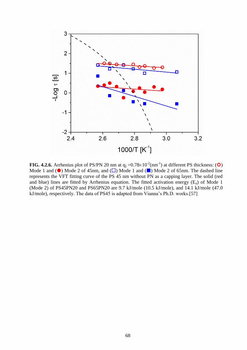
68
FIG. 4.2.6. Arrhenius plot of PS/PN 20 nm at q|| =0.7810-2
(nm-1
) at different PS thickness: ()
Mode 1 and () Mode 2 of 45nm, and () Mode 1 and () Mode 2 of 65nm. The dashed line
represents the VFT fitting curve of the PS 45 nm without PN as a capping layer. The solid (red
and blue) lines are fitted by Arrhenius equation. The fitted activation energy (Ea) of Mode 1
(Mode 2) of PS45PN20 and PS65PN20 are 9.7 kJ/mole (10.5 kJ/mole), and 14.1 kJ/mole (47.0
kJ/mole), respectively. The data of PS45 is adapted from Vianna’s Ph.D. works.[57]

69
FIG. 4.2.7. The q||-dependence of the mean relaxation rate for () PS 45 nm (black dashed
line) and Mode 2 of PS 45nm/ PN at 366K at different PN thickness: () 10 nm, () 20 nm,
and () 30 nm. The data of PS45 is adapted from Vianna’s Ph.D. works.[57]
To examine the contribution of the PS layer to the signal, in cooperation with the group of
Professor Dr. Friedrich Kremer at the Leipzig University, dielectric spectroscopy measurements
were conducted by this group on samples we prepared. The dielectric data shows that the α-
relaxation of the PS 45 nm is close to the bulk PS but seems to be somewhat faster – this could
be due to measuring different observables in dielectric spectroscopy and in mechanical
spectroscopy. Another possibility is that the faster segmental motions are induced by the density
fluctuation of polymer chains adjacent to the substrate [143]. This density fluctuation close to
the substrate influences the dynamics of the thin film more with decreasing film thickness. The
PS45PN30 follows a similar VFT curves as the PS 45 nm and bulk PS (FIG. 4.2.8) but is faster
than the bulk PS. This indicates the α-relaxation is probably not affected by the film thickness,
which is consistent with previous studies[7,11] of the Kremer group. Hence, for the Mode 1 and
Mode 2, we can neglect the contribution from the α-relaxation of the PS layer to the signal.

70
Our current results are in good agreement with the previous work[24] where it was found that
there is no Tg shift without a free surface. The PS thin film used here is confined between PN
and gold substrate, meaning that a free surface of the PS facing to the air does not exist. Since
the α-relaxation is a main indicator for Tg because it is the motion of polymer segments, the not
changing α-relaxation in our experiment agrees with a not shifted Tg. However, it should be
noted that the fluorescence studies[9,144] show different results.
In cooperation with the group of Dr. Eichhorn at the Leibniz Institute of Polymer Research
Dresden , temperature dependent ellipsometry experiments were performed on samples prepared
by us by our preparation method. Tg of 326K for PS 45 nm and PS45PN20 measured by the
ellipsometry (FIG. 4.2.9) are the same as the bulk PS measured by differential scanning
calorimetry. As is shown above, Tg is dictated by the α-relaxation and vice versa, and the α-
relaxation does not change in the thin film or bulk (FIG. 4.2.8). From this, we may expect that
there is no shift of Tg observed in the ellipsometric measurement. This was observed in the
ellipsometry measurement, indicating that our conclusion obtained from dielectric spectroscopy
and ellipsometric measurement is consistent. Furthermore, no shift in Tg also implies that the PS
under the PN layer has not been cross-linked during plasma polymerization process of
norborene on top of the PS surface.
When the polymer is cross-linked, the polymer chains are confined in smaller spaces than in
the not cross-linked situation. The activation or Arrhenius plot of cross-linked polymer shows
the Arrhenius behavior but not VFT behavior[145]. But it was reported[109] that plasma
polymerization generated tiny cross-linked part between the PS and PN layers. This hints to the
conclusion that the signal of Mode 1 and Mode 2 may be contributed from the PS/PN interface.

71
FIG. 4.2.8. Arrhenius plot of () PS Bulk, () PS 45 nm, () PS45PN30. The PS bulk is
measured by rheometer in a dynamic mechanical spectroscopy experiment[57] and the PS 45
nm and PS45PN30 were measured by dielectric spectroscopy. The solid line represents the VFT
curve of PS 45 nm measured by dielectric spectroscopy.

72
FIG. 4.2.9. The film thickness measured by ellipsometry as function of temperature for (a) PS
45 nm and (b) PS45PN20. The insets show the second derivatives of the temperature dependent
film thickness to determine precisely Tg. The black solid lines represent the fitting lines, and the
red dashed lines mark the Tg.
4.2.2 Discussion
The above results (FIG. 4.2.8 and 4.2.9) indicate that the contribution of α-relaxation of the
PS for Mode 1 and Mode 2 can be excluded from the signal we observe. These modes show
Arrhenius, i.e. thermally activated, behavior. This is an indication for a local mode. However,

73
the β-relaxation of the glass transition (cp. section 2.1) is one of the possible explanations for
the signal since the Mode 1 and Mode 2 show an Arrhenius curves which is typically found for
the β-relaxation process. Compared to the literature[141,142,146], both of the Mode 1 and Mode
2 locate in the range of 0.001 s to 10 s which is considered to be dominated by β-relaxation. The
β-relaxation can be found below Tg. When the temperature is above Tg, the β-relaxation
disappears or merges into the α-relaxation. However, both Mode 1 and Mode 2 can be observed
below Tg and extend over Tg (FIG. 4.2.5 and 4.2.6). In some cases the β-relaxation is regarded
as the side chain rotation[64] or side chain motion in general. In terms of polarization, dynamic
light scattering with the geometry of the incident orthogonal polarized to the scattered light can
capture the rotational motion (Section 3.2)[96,147]. But, for our PS thin films, we cannot see
any depolarized signal in the correlation functions. That indicates that rotation motion has only
negligible contribution to the Mode 1 and Mode 2.
The fragility index m, is defined as m= d(log τ)/d(Tg/T) and determined at Tg[67,148].
Because our curves, log τis very insensitive to the temperature, Tg/T (FIG. 4.2.6), the index m
can be considered as the average slope of different temperature. In the literature[140], the
segmental dynamics of polymers which refers to the motions of two to three polymer segments
confined in the nanoporous alumina (AAO) shows a so called “fragile” dynamic behavior when
the diameters of AAO are 200 and 400 nm. When the diameter of AAO is below 65 nm, the
segmental dynamics changes to the “strong” dynamic behavior. The AAO diameter of 65 nm is
a critical value for this fragile-to-strong transition. This means if the confined space is small
enough, the dynamics inside the polymer chains will be affected. Our results (FIG. 4.2.5 and
4.2.6) show a similar transition as reported in the literature[140], but do not show the typical α-
and β-relaxation behavior. The activation energy of Mode 2 increases with the thickness of the
PS increasing (FIG. 4.2.6). Hence, the Mode 2 can be attributed to a contribution from the
suppressed capillary wave. The stored energy is caused by the fluid deformation. When the
shape of the wave is deformed, the energy is dissipated into the PS layer. The specific motion
74
which cannot be found in the bulk possibly arises from the interface of polymer/polymer or
polymer/air[149]. Like internal waves in the ocean[150,151], if there is a surface tension
fluctuation at or in the PS/PN interface, the capillary wave can still exist there[76].
Addressing the question why we see Mode 1 and Mode 2 as local modes one can use in
analogy to the α-process of the glass transition the fragility index m as an indication for
characteristic length scales. m of Mode 1 of PS45PN20 and PS65PN20 are 1.5 and 2.3,
respectively. Recently the dynamics of CRR in thin films was shown[125]. According to the
literature[66,68], the fragility index is proportional to the size of the CRR (V) which is
introduced by Adam and Gibbs[65]. The fragility index and volume of CRR of bulk PS are
reported as 139 and 15.6 (nm3)[148,152], respectively. By using the Adam and Gibbs[65]
relation of the CRR, V=ξ3, the volume of CRR of Mode 1 can be estimated to 0.2 nm
3 with the
characteristic length ξ of 0.6 nm. The activation energy of Mode 1 is about 10 ~ 14 kJ/mol. Its
activation energy is less than the value of Ea ~ 60 kJ/mol of β-relaxation[141]. Larger activation
energy is related to a bigger size of the CRR[68]. This indicates the energy barrier the Mode 1
has to overcome is even less than the side chain rotation.
In another words, the length scale in which the polymer chains with the Mode 1 can move is
smaller than that for side chain rotation. For Mode 2 of PS65PN20, the index m is about 7.5, and
the characteristic length ξ can be estimated as 0.9 nm. The CRR of Mode 2 can be calculated
as 0.7 nm3
by using the Adam-Gibbs relation expressed above. On the other hand, the
characteristic length ξ ranges from 1 to 4 nm near Tg[9,153], giving the CRR of 1-64 nm3.
Thus, the CRRs of Mode 1 and Mode 2 are not large enough to affect the CRR near Tg. Hence,
it will be reasonable to anticipate that Tg of PS/PN samples is very similar to Tg of the bulk PS.
This fact also hints the properties of the Mode 1 and Mode 2; since the Mode 1 and Mode 2 are
not related to the bulk properties, these modes should arise from an extremely confined
environment such as the PS/PN interface.

75
The PN layer is assumed to be immobile in our experimental time scale (> 100 s). As
discussed above, both α- and β-relaxation can be excluded from the signal. At the PS/PN and
Au/PS interface, the layers are influenced by strong, attractive interactions (see Section 3.1),
and thus a possible slip effect is negligible. As also discussed above, the Mode 2 can be assumed
to be induced by the suppressed capillary wave. The dynamic length scale of Mode 1 is around
the scale of 4~5 polymer segments. However, Hu et. al[134] reported that mixed PS/PBrS layer
is present at the interface of the PS/PBrS bilayer system and showed extremely low viscosity.
This means that the mixed layer is very mobile. Furthermore, other studies[10,12,15,17,26]
have reported that there is a more mobile layer existing at the surface of the thin film. As shown
in Section 4.1, the surface of PB thin films has extremely low viscosity[123].
4.2.3 Summary
In this section, we characterized the capillary wave and its suppression of the PS/PN bilayer by
using the REDLS. The data show that the capillary wave at the PS surface confined between the
gold substrate and PN when the thickness of PN 20 nm and more. In this strongly confined
polymer sample of PS/PN bilayer, the PS shows a Arrhenius behavior even above Tg. In contrast
to the single-exponential decay found in the PS layer, the measured correlation function in the
confined PS/PN bilayer shows bi-exponential decay mode. This can be well accounted for by
using the theoretical model of multi-decay in the viscoelastic layer and bilayer[149]. We
demonstrated that the α-relaxation is not affected by the confinement, whereas the dynamics of
polymer chains near the interface is strongly affected. This is in a good agreement with the
literature[154]. Our data also implies that due to the strong attractive force acting on the PS/PN
interface, the interface plays an important role like PS and PN layers, and contributes to the
dynamics of the thin film.

76
4.3 Polystyrene thin films anchored to gold by thiol group
Evan et al.[13] explored the surface dynamics of a PS top layer in bilayer films and found that
the dynamics of the bilayer can be adjusted by changing the modulus of the sub-layer. When the
temperature is ~10K above the Tg of the PS top layer, the shorter relaxation time of PS top layer
with lower modulus sub-layer was shown, especially at the low in-plane scattering wave vector
(larger probing length scale). In addition, the relaxation time of PS top layer increases
significantly with decreasing PS top layer thickness. When the temperature is 40K above the Tg
of PS, the faster relaxation induced by the softer sub-layer and the stronger confinement effects
with decreasing thickness are neglected.
To get a better insight into the effects of confinement imposed by the solid substrate we
changed the interaction between the solid substrate and the polymer thin film by putting an
anchor for the film to the substrate. This anchor consists of covalently bound PS by thiol groups
as end groups of the PS.
When the PS surface is capped by the PN layer, multi-mode decays emerge in the correlation
functions. As is clarified in the Section 4.2, Mode 2 is inferred as to be contributed from the
suppressed capillary wave of the PS. The Mode 1 of the PS/PN samples follows a Arrhenius
curve and can be found below Tg. The emergence of the Arrhenius curve for the Mode 1
indicates that Mode 1 is weakly temperature dependent and has the relatively small energy
barrier. Also from the discussion in Chapter 4, the dynamic length scale of the Mode 1 is around
the scale of 4~5 polymer segments, and should arise from the PS/PN interface. Thus, we can
attribute the origin of the Mode 1 to the local motion at the PS/PN interface.
By measuring the capillary wave with XPCS[7,41], the surface viscosity of PS thin film was
found to be similar to the bulk PS. However, there is a more mobile layer with low viscosity
claimed to be at the surface of PS thin films[16]. For the PS thin film, an Arrhenius curve has
been reported[10,146] below Tg while above Tg, this Arrhenius curve disappears and/or merges

77
into the VFT curve. As the discussion about the Mode 1, this Arrhenius curve can be seen as the
thermal behavior of local motion. As such, it is reasonable to infer the more mobile layer to be
contributed from other kinds of the motion such as the local motion rather than capillary waves.
This inference can be supported by the reduction of local viscosity[31].
The contribution of the Mode 1 to the signal is assumed to be so tiny that Mode 1 cannot be
measured by REDLS and is hidden in the noise of the strong signal of the capillary wave.
Although the theoretical studies[149,155] predicted that multi-mode decays are present at the
single viscoelastic layer and the bilayer e.g. PS thin film and PS/PN thin film, whether a decay
can be observed or not really depends on the amplitude of the mode. Thus, the key point is that
the amplitude of the Mode 1 should be increased if possible or to lower or diminish the
amplitude of capillary waves as we did in the case of PS/PN to enable us to receive the signals
from the Mode 1.
Since the capillary wave is influenced by the properties of the viscoelastic layer[46], we want
to increase viscoelasticity of the PS layer by enhancing the confinement form the substrate. To
do this, we grafted the PS with a thiol end group (PS-SH) to the gold substrate, giving rise to an
increase in the viscoelasticity of the PS layer. This PS-SH forms an anchor to the PS spin-coated
subsequently and changes the adhesion and interaction of the PS with the substrate.
4.3.1 Results and discussion
Besides van der Waals force, there is no special interaction between the Au interface and PS.
After modifying the interface by grafting PS-SH, the binding of the interface to PS becomes
stronger.
Producing our films with unchanged experimental procedures as spinning speed and
concentration of the polymer solution, we found that the film thickness increased about 10 nm
on the Au interface modified by PS-SH. If the substrate becomes more binding to the PS in the
sample solution, more PS will be attached to the substrate at a fixed spinning-speed. Thus, the

78
increasing thickness at a fixed spinning-speed gives us the message that the confinement
between the Au and PS was enhanced.
To check for the attachment of PS-SH we performed AFM. All the samples were measured
with contact mode at 298K under 1 atm in air (Dimension 3100, Digital Instruments). The small
protrusion-like structures (FIG. 4.3.1c, d) are the PS-SH. PS-SH can be checked by the AFM
phase image (FIG. 4.3.1d). The molecular weight of our PS-SH is 3000 g/mole, and thus its
radius of gyration (Rg) is about 2 nm[106]. The profile (FIG. 4.3.2b) shows the height
difference equals to 2 nm, which is another evidence to confirm that the protrusions are PS-SH.
FIG. 4.3.1. AFM measurement (500nm500nm) at 298K for pure Au: (a) topography image (b)
phase image. PS-SH grafted to Au: (c) topography image (d) phase image. Comparing (a) and
(c), there are protrusion-like structures shown on the Au substrate after grafting the PS-SH. This
can be confirmed by the (d) since the PS-SH shows a different phase compared to the Au
substrate. The white and shiny spot in the (c) could be stemming from small impurities in the
solvent.

79
The Au layer was evaporated to the glass directly, and is composed of many different Au
facets inside (FIG 4.3.1a, b). Since thiol groups strongly graft to the [111] facets [156-158], the
PS-SH are only located at specific areas of the Au surface (FIG. 4.3.1c, d).
FIG. 4.3.2. AFM measurement (500nm500nm) at room temperature (a) for topography image
of PS-SH anchored to Au (b) profiles for the marked position 1 and 2.
FIG. 4.3.3. Schematics for Au which is modified by the PS-SH, and the PS layer is spin-coated
on the top of the PS-SH. The dark blue represents the PS layer here is less mobile.
The PS 35 nm grafted to gold substrate shows the Arrhenius behavior at T < Tg and T >
Tg+30K (FIG. 4.3.4). The time scales of Mode 1 and Mode 2 coincide with the temperature
region of T > Tg+30K and T < Tg, respectively (FIG. 4.3.4). At Tg < T < Tg+30K, the PS thin

80
film changes from the glassy state to the rubber state with increasing temperature. During this
phase transition, the polymer chains have to overcome a higher energy barrier, and this is related
to the larger size of the CRR. Hence, the dynamics of thin film is dominated by the capillary
wave. Compared to the PS 45 nm, the PS-SH/PS35 the relaxation changes from VFT to
Arrhenius dependence. This indicates that this mode of the PS-SH/PS35 moves locally because
of the strong confinement from the substrate. Over Tg + 30K, the dynamics of capillary wave
synchronized with the Mode 1. In the high T region, the cooperative length are also
reduced[146]. Decreasing cooperative length and increasing in confinement lowers the
amplitude of capillary wave, and makes the Mode 1 observable[149]. The PS-SH results fit with
the assumption about Mode 1. That manifests that the Mode 1 arises from the local motions at
the surface of the PS thin film.
FIG. 4.3.4. Comparison between films with PS capped by PN and the thiol anchored PS films.
Arrhenius plot measured at q|| = 0.78 10-2
(nm-1
) of () PS-SH/PS35, and () Mode 1 and ()
Mode 2 of PS45PN20. The dash-dot and solid lines represent the VFT curve of the capillary
waves of the PS 45 nm and the bulk, respectively. The data of PS45 and PS bulk are adapted
from Vianna’s Ph.D. works.[57]

81
The chain dynamics which corresponds to the end-to-end vector of polymer chains or of
terminal sub-chains are strongly affected by their boundary condition[154]. But the segmental
dynamics which length scale is referred to two to three polymer segments and hindered in the
bulk part of thin film is not affected by the boundary condition. The free end groups of chains
exist at the edge of polymer thin film[1]. These free end groups should move locally. The Mode
1 in our work might be referred to the motions of free end group at the edge.
The relaxation time of PS-SH/PS85 thin film decreased with increasing temperature
(FIG. 4.3.5). This trend is as predicted by the capillary wave model[2,20] since the surface
tension decreases with increasing temperature.
FIG. 4.3.5. Normalized, heterodyne auto-correlation functions for PS-SH/PS85 at q|| =0.7810-2
(nm-1
) and different temperatures: () 366K, () 378K, () 389K and () 398K. The solid
(red) lines are fits by KWW functions.
The PS-SH/PS65 shows the Arrhenius behavior at the temperature over Tg + 30K (FIG. 4.3.6).
When the PS thickness increases to the 85 nm (PS-SH/PS85), the VFT curve is shown at the
temperature over Tg + 30K (FIG. 4.3.6). That represents the capillary wave is not suppressed by

82
the confinement from the substrate. When the thin film becomes thicker, the surface is away
from and less confined from the substrate. Below Tg, there are Arrhenius curves like the Mode 1
in the PS/PN samples. The relaxation time of these Arrhenius curves decrease with increasing
thickness. Hence, these Arrhenius curves should originate from the surface and represent the
local motion.
FIG. 4.3.6. Arrhenius plot, q|| =0.7810-2
(nm-1
), of PS-SH/PS at different PS thickness: () 35
nm, () 65 nm and () 85 nm. For PS-SH/PS85, the VFT curve is shown from Tg + 30K. For
PS-SH/PS35 and PS-SH/PS65, the VFT curves are shown from Tg to Tg + 30K.
The relaxation time decreases with increasing scattering wave vector in the region q || >
0.56 x 10⁻²
nm-1
(marked by vertical dashed line) (FIG. 4.3.7). This trend is consistent with the
prediction of the capillary wave model. In the region of q|| < 0.56 x 10⁻²
nm-1
, the relaxation time
does not show the q||-dependent behavior due to the enhanced confinement from the substrate.
This transition can be thought as a transfer from internal interaction dominated (high q||, which is
referred to smaller probing length scale ) to a substrate dominated regime (low q ||, which is
referred to larger probing length scale )[123]. The transition is not related to the modulus of the

83
thin film itself since PS-SH/PS85 shows the same transition q|| at different temperature.
Compared to the literature[123], this transition shifts to lower q|| because the enhanced
confinement. That also means the enhanced confinement from the substrate does not affect the
internal interaction of polymer chains (high q|| ).
FIG. 4.3.7. q||-dependent relaxation time of PS-SH/PS85 at different temperature: () 366K,
() 378K, () 389K and () 398K.
The viscosities of the PS-SH/PS85 obtained from the fit decreased with increasing temperature
(FIG. 4.3.8b). Their value was higher than bulk value about half order. According to the
literatures[7,41], the viscosity of PS thin films should be the same as the bulk. Hence, the bulk
viscosities of different temperatures were regarded as defaults in the capillary wave model to fit
and get the related effective thickness (TABLE 4.3.2). The effective thickness is defined as the
thickness of the part of the thin film contributing to the capillary wave motion according to the
fit result. The effective thickness is about 30 nm at all temperatures (FIG. 4.3.9b). 85 nm of PS
was spin-coated on the Au modified by PS-SH. Therefore there is about 55 nm thick PS layer
strongly confined by the substrate and which effectively does not contribute the dynamics of
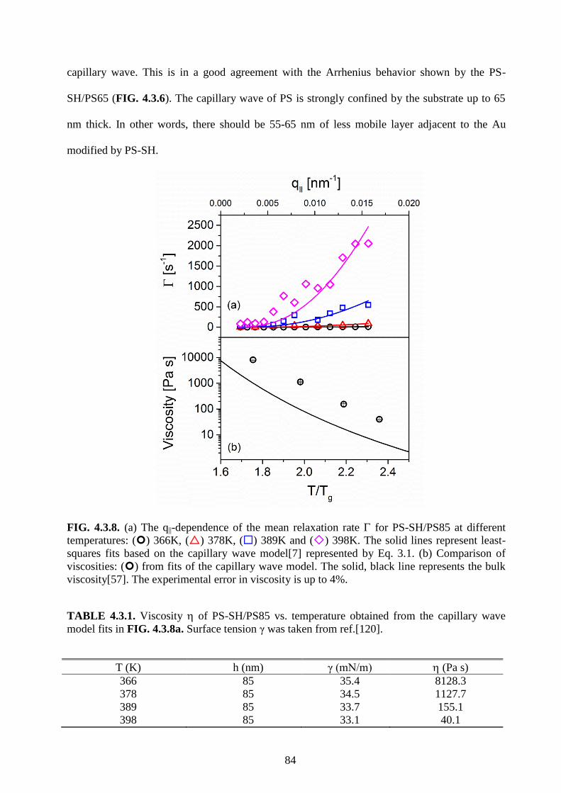
84
capillary wave. This is in a good agreement with the Arrhenius behavior shown by the PS-
SH/PS65 (FIG. 4.3.6). The capillary wave of PS is strongly confined by the substrate up to 65
nm thick. In other words, there should be 55-65 nm of less mobile layer adjacent to the Au
modified by PS-SH.
FIG. 4.3.8. (a) The q||-dependence of the mean relaxation rate for PS-SH/PS85 at different
temperatures: () 366K, () 378K, () 389K and () 398K. The solid lines represent least-
squares fits based on the capillary wave model[7] represented by Eq. 3.1. (b) Comparison of
viscosities: () from fits of the capillary wave model. The solid, black line represents the bulk
viscosity[57]. The experimental error in viscosity is up to 4%.
TABLE 4.3.1. Viscosity of PS-SH/PS85 vs. temperature obtained from the capillary wave
model fits in FIG. 4.3.8a. Surface tension γ was taken from ref.[120].
T (K) h (nm) γ (mN/m) (Pa s)
366 85 35.4 8128.3
378 85 34.5 1127.7
389 85 33.7 155.1
398 85 33.1 40.1

85
FIG. 4.3.9. (a) The q||-dependence of the mean relaxation rate for PS-SH/PS85 at different
temperatures: () 366K, () 378K, () 389K and () 398K. The solid lines represent least-
squares fits based on the capillary wave model[7] represented by Eq. 3.1. (b) (). Effective
thickness from fits of the capillary wave model. The red, dashed line represents the real
thickness of PS. The error in effective thickness is up to 12%.
TABLE 4.3.2. Effective thickness heff
of PS-SH/PS85 vs. temperature obtained from the
capillary wave model fits in FIG. 4.3.9a. Surface tension γ was taken from ref.[120].
T (K) Bulk (Pa s) γ (mN/m) heff
(nm)
366 1016.5 35.4 30.5
378 95.6 34.5 25.8
389 17 33.7 28.7
398 5.2 33.1 30.8

86
4.3.2 Summary
In this study, experiments on Au substrate modified by PS-SH which have been covered by
spin-coating with a PS layer on top are evaluated. By using the preparation method mentioned
above, the confinement from the substrate is enhanced, and the capillary wave is suppressed by
that. Since the amplitude of capillary wave is lowered by enhanced confinement from the
substrate, the Mode 1 which is discussed in Chapter 4 has been confirmed to originate from the
local motion at the surface of the PS thin film. The capillary wave is strongly confined in the
larger probing length scale (low qll). The effective thickness which really contributes to the
capillary wave is less than the real thickness of PS on the top of the substrate. Because the
confinement from the substrate is enhanced, the length scale of less mobile layer adjacent to the
substrate increases. This viscoelastic layer does not contribute to the motions of capillary wave,
and makes the viscosity of PS-SH/PS samples increasing. As such, we demonstrated that the
surface dynamics can be tuned by the interaction between the substrate and polymer which can
be change by modifying the substrate.

87
Chapter 5
Conclusion
In this thesis, the noninvasive and marker-free experimental method REDLS was employed to
measure the dynamics of polymer thin films of which capillary waves were the most prominent
ones. Based on a study of the capillary waves of PS thin films[57], we want to go further to
investigate how capillary waves behave in different confinement situation and temperature
region, e.g., close to the Tg or far above Tg in low viscosity, liquid-like thin films. Thus, three
different systems have been measured:
(1) Low viscosity, liquid-like thin film, PB, at temperature of Tg + 125K
(2) PS/PN bilayers, measured at temperature close to Tg in order to study the capillary waves
of PS thin films strongly suppressed by a glassy PN layer.
(3) PS thin films anchored to the substrate of gold by thiol group to enhance the confinement
from the substrate to suppress the capillary waves to figure out the possible motion
modes of polymer chains at the thin film surface.
In the first part of my thesis, I measured capillary waves of the PB thin films in different wave
vectors and thicknesses. A three layer model to explain the dynamics of polymer thin films
changing with thickness was introduced to explain the findings. I also showed that the effective
length scale of the confinement from the substrate is a fixed distance of about 20-25 nm not
related to the 3Rg postulated in literature before.
The three layer model proposed is composed by: a less mobile layer compared to the mobility
in the same bulk polymer adjacent to the substrate, a more mobile layer at the polymer/air
surface, and the remaining bulk part. The viscosity of polymer thin film at different thickness is
determined by the ratio of less mobile, more mobile, and bulk layer. The three layer model
means the polymer thin film is heterogeneous and shows a distribution of dynamics which is

88
qualitatively in agreement to a prediction by de Gennes[1]. The influence of less mobile and
more mobile layers makes the dynamics of polymer thin film different from the bulk as seen by
most experiments observing the film as a whole as e.g. dielectric spectroscopy.
In the second part of my thesis, a glassy PN layer was polymerized on the top of PS thin film
directly by plasma polymerization to suppress capillary waves by this capping. I found that the
thermal behavior of capillary waves is changing from a non-Arrhenius behavior to Arrhenius
behavior. When we put PN layers with thickness over 20 nm on the top of the PS thin film,
capillary waves are strongly suppressed by this solid, glassy PN layer. The amplitude of
capillary waves is lowered because of this strong suppression. But, we found that the Tg and the
α-relaxation of our polymer thin films are not affected by the PN layer and are similar to the
bulk.
This lowered amplitude is what makes it possible to observe a local motion which relaxation
time is shorter than the capillary wave at the surface of polymer thin film. This local motion is
faster than the α-relaxation and is also not affected by the confinement from the substrate or the
thickness of PN layer.
In the third part of my thesis, I anchored the PS thin film to Au by thiol group. Through this
enhanced confinement from the substrate, the thickness of the less mobile layer is enlarged and
suppresses the capillary wave via a change in the viscoelastic behavior. If we do not change the
interaction between the substrate and polymer to enhance or weaken the confinement from the
substrate, the thickness of the less mobile layer at a temperature of Tg + 125K should be limited
to a fixed distance not related to the 3Rg. But, the substrate modified by the anchor molecules
enhances the confinement and enlarges the effective length scale of the less mobile layer and
increases the viscosity of polymer thin film. Hence, the dynamics of polymer thin film can be
tuned by modifying the substrate.
The confinement from the substrate will induce a more dense layer of a few nm adjacent to the
substrate[32,33] and thus this region has smaller free volume as reported in a combination of
89
molecular dynamic simulation and PALS[35]. This more dense layer of a few nm probably
induces changes in the mobility and leads to the less mobile layer of 20-25 nm mentioned in the
three layer model. But the connection of the more dense layer and the less mobile layer is still an
open question.
Based on the above results and discussions, there are some unsolved questions of glass
transition in nanoscale which need to be answered in the future.
First, polymer thin films show heterogeneous dynamics along the different depth rather than a
simple homogeneous layer. The capillary wave model based on a homogeneous single layer is
applied to get the viscosity of polymer thin film. Compared to the bulk, we get one order of
magnitude lower viscosities in the PB thin films and half an order of magnitude higher
viscosities in the PS-SH/PS thin films. A modification of the capillary wave model by
considering the film to be composed of several layers seems to be necessary.
Second, the effective length scale of confinement from the substrate should be limited to few
nm away from the substrate i.e., the thickness of dense layer is no more than 2 nm. However, the
length scale of the less mobile layer is much more. Moreover, the less mobile layer affects the
capillary wave of polymer thin film. What is the mechanism for the dense layer to become the
less mobile layer? What is the long range relation between the capillary wave and less mobile
layer?
Third, the more mobile layer is proven to exist at the surface of polymer thin films and the
main reason inducing for the reported reductions of Tg with decreasing film thickness. But, what
kind of motion induces the more mobile layer? What is the effective length scale of these
motions contributing to the more mobile layer?
90
List of abbreviations
Tg Glass transition temperature
η Viscosity
PS Polystyrene
h Film thickness
AFM Atomic force microscopy
NMR Nuclear Magnetic resonance
Mw Molecular weight
XPCS X-ray photon correlation spectroscopy
Rg Radius of gyration
PB Polybutadiene
PI cis-Polyisoprene
CRR Co-operative rearrange region
ξ(T) Temperature dependent length scale
REDLS Resonance enhanced dynamic light scattering
PN Polynorbornene
DLS Dynamic light scattering
SPP Surface plasma polariton
SPR Surface plasma resonance spectroscopy
np Refractive index of prism
nd Refractive index of dielectric medium
θc Critical angle for total reflection
εp Dielectric constant for prism
εd Dielectric constant for dielectric medium

91
Γ Relaxation rate
q Scattering wave vector
n Refractive index
λ Wave length of incident light
ki Wave vector of incident light
ks Wave vector of scattered light
KWW Kohlrausch-Williams-Watts equation
β Stretching parameter
τ Relaxation time
VFT Vogel-Fulcher-Tammam
qll In-plane scattering wave vector
PS-SH Polystyrene modified by thiol group
rms Roughness
Ea Activation energy
m Fragility index
V Size of the co-operative rearrange region
γ Surface tension
heff
Effective thickness

92
References
[1] P. De Gennes, The European Physical Journal E: Soft Matter and Biological Physics 2,
201 (2000).
[2] S. Herminghaus, The European Physical Journal E: Soft Matter and Biological Physics 8,
237 (2002).
[3] L. Yelash, P. Virnau, K. Binder, and W. Paul, Physical Review E 82, 4, 050801 (2010).
[4] L. Yelash, P. Virnau, K. Binder, and W. Paul, Epl 98, 5, 28006 (2012).
[5] S. Herminghaus, K. Jacobs, and R. Seemann, The European Physical Journal E 5, 531
(2001).
[6] K. Ngai, The European Physical Journal E 8, 225 (2002).
[7] H. Kim, A. Rühm, L. Lurio, J. Basu, J. Lal, D. Lumma, S. Mochrie, and S. Sinha,
Physical Review Letters 90, 68302 (2003).
[8] J. Keddie, R. Jones, and R. Cory, EPL (Europhysics Letters) 27, 59 (1994).
[9] C. J. Ellison and J. M. Torkelson, Nature Materials 2, 695 (2003).
[10] Z. Fakhraai and J. Forrest, Science 319, 600 (2008).
[11] M. Tress et al., Macromolecules 43, 9937 (2010).
[12] K. Paeng, R. Richert, and M. Ediger, Soft Matter 8, 819 (2012).
[13] C. M. Evans, S. Narayanan, Z. Jiang, and J. M. Torkelson, Physical Review Letters 109,
038302 (2012).
[14] K. J. Alvine, Y. Dai, H. W. Ro, S. Narayanan, A. Sandy, C. L. Soles, and O. G. Shpyrko,
Physical Review Letters 109, 207801 (2012).
[15] Y. Chai, T. Salez, J. D. McGraw, M. Benzaquen, K. Dalnoki-Veress, E. Raphaël, and J.
A. Forrest, Science 343, 994 (2014).
[16] M. Ediger and J. Forrest, Macromolecules 47, 471 (2013).
[17] K. Paeng, S. F. Swallen, and M. D. Ediger, Journal of the American Chemical Society
(2011).
[18] J. Harden, H. Pleiner, and P. Pincus, The Journal of chemical physics 94, 5208 (1991).
[19] J. Jackle and K. Kawasaki, Journal of Physics: condensed matter 7, 4351 (1995).
[20] J. Jäckle, Journal of Physics: Condensed Matter 10, 7121 (1998).
[21] J. H. Kim, J. Jang, and W.-C. Zin, Langmuir 16, 4064 (2000).
[22] S. Kawana and R. A. Jones, Physical Review E 63, 021501 (2001).
[23] O. Bäumchen, J. McGraw, J. Forrest, and K. Dalnoki-Veress, Physical Review Letters
109, 55701 (2012).
[24] J. Sharp and J. Forrest, Physical Review Letters 91, 235701 (2003).
[25] M. Y. Efremov, A. V. Kiyanova, J. Last, S. S. Soofi, C. Thode, and P. F. Nealey,
Physical Review E 86, 021501 (2012).
[26] Z. Yang, Y. Fujii, F. K. Lee, C.-H. Lam, and O. K. Tsui, Science 328, 1676 (2010).
[27] G. Reiter, in Glass Transition, Dynamics and Heterogeneity of Polymer Thin Films
(Springer, 2013), pp. 29.
[28] S. Herminghaus, R. Seemann, and K. Landfester, Physical review letters 93, 017801
(2004).
[29] M. Tress, E. U. Mapesa, W. Kossack, W. K. Kipnusu, M. Reiche, and F. Kremer,
Science 341, 1371 (2013).
[30] F. Kremer, M. Tress, and E. U. Mapesa, Journal of Non-Crystalline Solids (2014).
[31] T. Koga, C. Li, M. Endoh, J. Koo, M. Rafailovich, S. Narayanan, D. Lee, L. Lurio, and S.
Sinha, Physical review letters 104, 066101 (2010).
93
[32] K. Johnston and V. Harmandaris, Soft Matter (2012).
[33] K. Johnston and V. Harmandaris, Macromolecules 46, 5741 (2013).
[34] M. Solar, E. Mapesa, F. Kremer, K. Binder, and W. Paul, EPL (Europhysics Letters) 104,
66004 (2013).
[35] H. J. Butt et al., Macromolecules 47, 8459 (2014).
[36] J. D. McCoy and J. G. Curro, The Journal of chemical physics 116, 9154 (2002).
[37] C. Batistakis, A. V. Lyulin, and M. Michels, Macromolecules 45, 7282 (2012).
[38] A. Papon, H. Montes, M. Hanafi, F. Lequeux, L. Guy, and K. Saalwächter, Physical
review letters 108, 065702 (2012).
[39] J. Wang, M. Tolan, O. Seeck, S. Sinha, O. Bahr, M. Rafailovich, and J. Sokolov,
Physical Review Letters 83, 564 (1999).
[40] S. Narayanan, D. R. Lee, R. S. Guico, S. K. Sinha, and J. Wang, Physical review letters
94, 145504 (2005).
[41] Z. Jiang et al., Physical Review Letters 98, 227801 (2007).
[42] R. S. Guico, S. Narayanan, J. Wang, and K. R. Shull, Macromolecules 37, 8357 (2004).
[43] D. Qi, Z. Fakhraai, and J. Forrest, Physical Review Letters 101, 096101 (2008).
[44] D. Long and F. Lequeux, The European Physical Journal E 4, 371 (2001).
[45] F. Varnik, J. Baschnagel, and K. Binder, Physical Review E 65, 021507 (2002).
[46] A. Semenov, Physical Review Letters 80, 1908 (1998).
[47] S. Kim and J. M. Torkelson, Macromolecules (2011).
[48] J. E. Pye and C. B. Roth, Physical Review Letters 107, 235701 (2011).
[49] K. Paeng and M. Ediger, Macromolecules 44, 7034 (2011).
[50] D. Qi, M. Ilton, and J. Forrest, The European Physical Journal E: Soft Matter and
Biological Physics 34, 1 (2011).
[51] L. Zhu, C. Brian, S. Swallen, P. Straus, M. Ediger, and L. Yu, Physical Review Letters
106, 256103 (2011).
[52] C. R. Daley, Z. Fakhraai, M. D. Ediger, and J. A. Forrest, Soft Matter 8, 2206 (2012).
[53] S. Mirigian and K. S. Schweizer, The Journal of chemical physics 141, 161103 (2014).
[54] M. A. Plum, S. D. B. Vianna, A. Unger, R. F. Roskamp, H. J. Butt, B. Menges, and W.
Steffen, Soft Matter 7, 1501 (2011).
[55] M. A. Plum, B. Menges, G. Fytas, H.-J. Butt, and W. Steffen, Review of Scientific
Instruments 82, 015102 (2011).
[56] M. A. Plum, W. Steffen, G. Fytas, W. Knoll, and B. Menges, Optics Express 17, 10364
(2009).
[57] S. D. B. Vianna, Ph.D. Thesis (2012).
[58] R. D. Priestley, D. Cangialosi, and S. Napolitano, Journal of Non-Crystalline Solids 407,
288 (2015).
[59] H. Vogel, Phys. Z 22, 645 (1921).
[60] G. S. Fulcher, Journal of the American Ceramic Society 8, 339 (1925).
[61] G. Tammann and W. Hesse, Z. Anorg. Allg. Chem 156, 245 (1926).
[62] C. Angell, MRS bulletin 33, 544 (2008).
[63] A. J. Kovacs, in Fortschritte der Hochpolymeren-Forschung (Springer, 1964), pp. 394.
[64] F. Kremer and A. Schönhals, Broadband dielectric spectroscopy (Springer, 2003).
[65] G. Adam and J. H. Gibbs, The Journal of chemical physics 43, 139 (1965).
[66] A. Saiter, E. Dargent, J. Saiter, and J. Grenet, Journal of non-crystalline solids 354, 345
(2008).
[67] D. J. Plazek and K. L. Ngai, Macromolecules 24, 1222 (1991).
[68] C. A. Solunov, European polymer journal 35, 1543 (1999).
[69] C. Angell, Journal of Physics and Chemistry of Solids 49, 863 (1988).
[70] H. Tanaka, The Journal of chemical physics 105, 9375 (1996).
[71] J. A. Forrest and K. Dalnoki-Veress, ACS Macro Letters 3, 310 (2014).

94
[72] J. A. Forrest, The Journal of Chemical Physics 139 (2013).
[73] J. D. van der Waals, J Stat Phys 20, 200 (1979).
[74] M. Smoluchowski, Annalen der Physik 330, 205 (1908).
[75] L. Mandelstam, Annalen der Physik 346, 609 (1913).
[76] V. Levich and V. Krylov, Annual Review of Fluid Mechanics 1, 293 (1969).
[77] F. Buff, R. Lovett, and F. Stillinger, Physical Review Letters 15, 621 (1965).
[78] L. P. Kadanoff and P. C. Martin, Annals of Physics 24, 419 (1963).
[79] A. Braslau, M. Deutsch, P. Pershan, A. Weiss, J. Als-Nielsen, and J. Bohr, Physical
Review Letters 54, 114 (1985).
[80] M. Sanyal, S. Sinha, K. Huang, and B. Ocko, Physical Review Letters 66, 628 (1991).
[81] B. Ocko, X. Wu, E. Sirota, S. Sinha, and M. Deutsch, Physical Review Letters 72, 242
(1994).
[82] T. Seydel, M. Tolan, B. Ocko, O. Seeck, R. Weber, E. DiMasi, and W. Press, Physical
Review B 65, 184207 (2002).
[83] S. K. Sinha, E. Sirota, S. Garoff, and H. Stanley, Physical Review B 38, 2297 (1988).
[84] T. Seydel, A. Madsen, M. Tolan, G. Grübel, and W. Press, Physical Review B 63,
073409 (2001).
[85] A. Madsen, J. Als-Nielsen, and G. Grübel, Physical Review Letters 90, 085701 (2003).
[86] T. Seydel, A. Madsen, M. Sprung, M. Tolan, G. Grübel, and W. Press, Review of
Scientific Instruments 74, 4033 (2003).
[87] C. Gutt, T. Ghaderi, V. Chamard, A. Madsen, T. Seydel, M. Tolan, M. Sprung, G.
Grübel, and S. Sinha, Physical Review Letters 91, 179902 (2003).
[88] C. Gutt, T. Ghaderi, V. Chamard, A. Madsen, T. Seydel, M. Tolan, M. Sprung, G.
Grübel, and S. Sinha, Physical Review Letters 91, 76104 (2003).
[89] V. G. Levich, Physicochemical hydrodynamics (Prentice-Hall Englewood Cliffs, NJ,
1962), Vol. 689.
[90] G. R. Strobl, The physics of polymers: concepts for understanding their structures and
behavior (Springer, 2007).
[91] N. Fatkullin, R. Kimmich, and M. Kroutieva, Journal of Experimental and Theoretical
Physics 91, 150 (2000).
[92] L. D. Landau and E. Lifshitz, Course of Theoretical Physics 3 (1986).
[93] L. Landau and E. Lifshitz, Course of Theoretical Physics, 227 (1987).
[94] F. Brochard-Wyart, P.-G. De Gennes, H. Hervert, and C. Redon, Langmuir 10, 1566
(1994).
[95] A. Madsen, T. Seydel, M. Sprung, C. Gutt, M. Tolan, and G. Grübel, Physical Review
Letters 92, 96104 (2004).
[96] B. J. Berne and R. Pecora, Dynamic light scattering: with applications to chemistry,
biology, and physics (Courier Dover Publications, 2000).
[97] L. Novotny and B. Hecht, Principles of nano-optics (Cambridge university press, 2012).
[98] H. Raether, Surface plasmons on smooth surfaces (Springer, 1988).
[99] W. Knoll, Annual Review of Physical Chemistry 49, 569 (1998).
[100] E. Kretschmann and H. Raether, Zeitschrift Fuer Naturforschung, Teil A 23, 2135 (1968).
[101] N. Bunjes, E. Schmidt, A. Jonczyk, F. Rippmann, D. Beyer, H. Ringsdorf, P. Gräber, W.
Knoll, and R. Naumann, Langmuir 13, 6188 (1997).
[102] A. Otto, Zeitschrift für Physik 216, 398 (1968).
[103] I. Pockrand, Surface Science 72, 577 (1978).
[104] E. T. Hoppe, I. Hopp, M. Port, B. Menges, and C. M. Papadakis, Colloid and Polymer
Science 290, 1731 (2012).
[105] J. C. Seferis, Polymer Handbook 4, 571 (1999).
[106] L. Fetters, N. Hadjichristidis, J. Lindner, and J. Mays, Journal of physical and chemical
reference data 23, 619 (1994).

95
[107] N. Sultanova, S. Kasarova, and I. Nikolov, Acta Physica Polonica-Series A General
Physics 19, 585 (2009).
[108] T. Kaule et al., ACS nano 7, 748 (2012).
[109] Y. Zhang, J. Arfsten, S. A. Pihan, T. Kaule, R. Förch, and R. Berger, Journal of colloid
and interface science 351, 532 (2010).
[110] L.-Q. Chu, W. Knoll, and R. Förch, Langmuir 22, 5548 (2006).
[111] M. A. Plum, Ph.D. Thesis (2010).
[112] F. Arecchi, M. Corti, V. Degiorgio, and S. Donati, Optics Communications 3, 284
(1971).
[113] D. E. Koppel, The Journal of Chemical Physics 57, 4814 (1972).
[114] C. Lindsey and G. Patterson, The Journal of Chemical Physics 73, 3348 (1980).
[115] S. W. Provencher, Die Makromolekulare Chemie 180, 201 (1979).
[116] S. W. Provencher, Computer Physics Communications 27, 213 (1982).
[117] R. Kohlrausch, Annalen der Physik 167, 179 (1854).
[118] G. Williams and D. C. Watts, Trans. Faraday Soc. 66, 80 (1970).
[119] W. Brown, Dynamic light scattering: the method and some applications (Oxford
University Press, USA, 1993), Vol. 49.
[120] D. W. Van Krevelen and K. Te Nijenhuis, Properties of polymers: their correlation with
chemical structure; their numerical estimation and prediction from additive group
contributions (Access Online via Elsevier, 2009).
[121] J. Gruver and G. Kraus, Journal of Polymer Science Part A: General Papers 2, 797
(1964).
[122] A. Hofmann, A. Alegria, J. Colmenero, L. Willner, E. Buscaglia, and N. Hadjichristidis,
Macromolecules 29, 129 (1996).
[123] F.-Y. Lin and W. Steffen, The Journal of Chemical Physics 141, 104903 (2014).
[124] M. J. Struglinski and W. W. Graessley, Macromolecules 18, 2630 (1985).
[125] H. K. Nguyen, D. Wang, T. P. Russell, and K. Nakajima, Soft Matter (2014).
[126] G. Vinogradov, Y. G. Yanovskii, E. Borisenkova, B. Yarlykov, and G. Berezhnaya,
Journal of Polymer Science Part A‐2: Polymer Physics 10, 1061 (1972).
[127] W. Rochefort, G. Smith, H. Rachapudy, V. Raju, and W. Graessley, Journal of Polymer
Science: Polymer Physics Edition 17, 1197 (1979).
[128] F. Stickel, E. W. Fischer, and R. Richert, The Journal of Chemical Physics 104, 2043
(1996).
[129] J. N. Israelachvili, Intermolecular and surface forces: revised third edition (Academic
press, 2011).
[130] P. S. Stephanou, C. Baig, G. Tsolou, V. G. Mavrantzas, and M. Kroeger, Journal of
Chemical Physics 132, 124904 (2010).
[131] C. D. Han and T. C. Yu, Journal of Applied Polymer Science 15, 1163 (1971).
[132] P. J. Cole, R. F. Cook, and C. W. Macosko, Macromolecules 36, 2808 (2003).
[133] R. Zhao and C. W. Macosko, Journal of Rheology (1978-present) 46, 145 (2002).
[134] X. Hu, Z. Jiang, S. Narayanan, X. Jiao, A. R. Sandy, S. K. Sinha, L. B. Lurio, and J. Lal,
Physical Review E 74, 010602 (2006).
[135] C.-P. Klages, A. Dietz, T. Höing, R. Thyen, A. Weber, and P. Willich, Surface and
Coatings Technology 80, 121 (1996).
[136] H. Sirringhaus, T. Kawase, R. Friend, T. Shimoda, M. Inbasekaran, W. Wu, and E. Woo,
Science 290, 2123 (2000).
[137] J. Zhang, C. M. Li, M. B. Chan-Park, Q. Zhou, Y. Gan, F. Qin, B. Ong, and T. Chen,
Applied physics letters 90, 243502 (2007).
[138] M. F. Weber, C. A. Stover, L. R. Gilbert, T. J. Nevitt, and A. J. Ouderkirk, Science 287,
2451 (2000).
96
[139] M. Ibanescu, Y. Fink, S. Fan, E. L. Thomas, and J. D. Joannopoulos, Science 289, 415
(2000).
[140] H. Duran, A. Gitsas, G. Floudas, M. Mondeshki, M. Steinhart, and W. Knoll,
Macromolecules 42, 2881 (2009).
[141] H. Lee, A. Jamieson, and R. Simha, Macromolecules 12, 329 (1979).
[142] J. Cavaille, C. Jourdan, J. Perez, L. Monnerie, and G. Johari, Journal of Polymer Science
Part B: Polymer Physics 25, 1235 (1987).
[143] Y. Suzuki, H. Duran, W. Akram, M. Steinhart, G. Floudas, and H.-J. Butt, Soft Matter 9,
9189 (2013).
[144] C. B. Roth, K. L. McNerny, W. F. Jager, and J. M. Torkelson, Macromolecules 40, 2568
(2007).
[145] N. Alves, G. Ribelles, G. Tejedor, and J. Mano, Macromolecules 37, 3735 (2004).
[146] Z. Fakhraai and J. A. Forrest, Physical Review Letters 95, 25701 (2005).
[147] M. Haghighi, M. A. Plum, G. Gantzounis, H.-J. Butt, W. Steffen, and G. Fytas, The
Journal of Physical Chemistry C 117, 8411 (2013).
[148] R. Böhmer, K. Ngai, C. Angell, and D. Plazek, The Journal of chemical physics 99, 4201
(1993).
[149] M. L. Henle and A. J. Levine, Physical Review E 75, 021604 (2007).
[150] J. R. Apel, An atlas of oceanic internal solitary waves (2002).
[151] C. Garrett and W. Munk, Annual Review of Fluid Mechanics 11, 339 (1979).
[152] E. Hempel, G. Hempel, A. Hensel, C. Schick, and E. Donth, The Journal of Physical
Chemistry B 104, 2460 (2000).
[153] C. J. Ellison, M. K. Mundra, and J. M. Torkelson, Macromolecules 38, 1767 (2005).
[154] E. U. Mapesa, M. Tress, G. Schulz, H. Huth, C. Schick, M. Reiche, and F. Kremer, Soft
Matter 9, 10592 (2013).
[155] P. M. Chaikin and T. C. Lubensky, Principles of condensed matter physics (Cambridge
Univ Press, 2000), Vol. 1.
[156] Z. Nie, D. Fava, E. Kumacheva, S. Zou, G. C. Walker, and M. Rubinstein, Nature
materials 6, 609 (2007).
[157] C. J. Murphy, T. K. Sau, A. M. Gole, C. J. Orendorff, J. Gao, L. Gou, S. E. Hunyadi, and
T. Li, The Journal of Physical Chemistry B 109, 13857 (2005).
[158] K. Caswell, J. N. Wilson, U. H. Bunz, and C. J. Murphy, Journal of the American
Chemical Society 125, 13914 (2003).