TESTING THE RISK RETURN RELATIONSHIP OF THE MUTUAL

FUNDS MARKET IN KENYA

By:

Kariuki Titus Thuo

D61/62447/2010

A Research Project Submitted in Partial Fulfilment of the Requirements

for the Award of Degree in Master of Business Administration, University

of Nairobi

2013

ii

DECLARATION

This research project is my original work and has not been submitted for the award of a

degree in any other university.

Titus Thuo Kariuki

Signed……………………………………………………

Date………………………………….

Registration Number: D61/62447/2010

This research project has been submitted for examination with my approval as a university

supervisor.

Dr. Josiah O Aduda.

Signed…………………………………………………….Date………………………………

iii

DEDICATION

I dedicate this research project to my loving family and friends who have been a constant

inspiration and encouragement while undertaking this project. I also dedicate it to the

University of Nairobi MBA fraternity for the knowledge imparted in me.

iv

ACKNOWLEDGEMENTS

I would like to acknowledge my supervisor Dr. Josiah O. Aduda for his guidance and insights

accorded to me while undertaking this study. His advice, comment and patience enabled me

to complete this project. I would also like to acknowledge my colleagues at the University of

Nairobi MBA School of business for their support, criticism and insights. Their constant

encouragement throughout the project cycle is invaluable.

I would also like to acknowledge the various mutual funds employees who assisted me with

data from their published financial records. I would like to acknowledge the assistance

obtained from Africa alliance investment bank, Commercial bank of Africa asset

management department, ICEA lion asset management, Zimele asset management, Standard

and investment bank for providing me with primary data from their records. I acknowledge

Britarm asset management, Commercial bank of Africa and old mutual asset management

who had their published financial results online for easy access. This project would not have

been accomplished without their input. Finally, I would also like to acknowledge my work

colleagues at Techno Brain limited for their moral support and assistance in proof reading the

various drafts of the proposal and final report. May our lord bless you all abundantly.

v

ABSTRACT

The growth in the mutual funds market in Kenya has led to great interest in the risk return

relationship in this market. Various asset pricing models can be utilized in empirical testing

to determine the dominant risk factors affecting returns. This study adopted the arbitrage

pricing model to identify and analyse these economic factors. The Treasury bill rate, GDP

growth rate, inflation size and the fund size were the independent variables selected for the

model whose beta parameters were analysed. The study was conducted for the period

between 2006 and 2012.

This study found that a positive relationship existed between mutual funds returns and the

Treasury bill rate and market interest rates. A negative beta was computed for GDP growth

rate, inflation rate and fund size factors. These factors represent risk in the mutual funds

market and a positive risk return relationship was computed from the model. Inflation rate,

market interest rates and GDP growth rate were observed to have the greatest impact on

mutual funds returns. The fund size had a lower but significant coefficient while the beta for

Treasury bill rate factor was insignificant.

The study found that expansionary economic policies, marketing and diversification business

strategies are necessary to manage economic risks that affect returns in the mutual funds

market.

vi

ABBREVIATIONS

AHP ……………….. Analytical Hierarchy Process

APT ……………….. Arbitrage Pricing Theory

CAPM………………. Capital Asset Pricing Model

CMA……………….. Capital Markets Authority

GDP………………….Gross Domestic Product

HMS……………….. High minus Low

SMB……………….. Small Minus Big

SPSS ……………….. Statistical Package for social Sciences

TB…………………….Treasury Bills

vii

TABLES

Table 1……………………………………Model Summary

Table 2…………………………………….ANOVA

Table 3……………………………………. Coefficients

Table 4…………………………………… Mutual funds data

Table 5…………………………………… Economic factors

viii

TABLE OF CONTENTS

DECLARATION .............................................................................................................................. ii

ACKNOWLEDGEMENTS .............................................................................................................. iv

ABSTRACT...................................................................................................................................... v

ABBREVIATIONS .......................................................................................................................... vi

TABLES ..........................................................................................................................................vii

CHAPTER ONE ............................................................................................................................... 1

INTRODUCTION ............................................................................................................................. 1

1.1 Background to the Study .................................................................................................... 1

1.1.1 Risk and Return .......................................................................................................... 2

1.2 Statement of the Problem ................................................................................................... 4

1.3 Objective of the Study ........................................................................................................ 6

1.4 Significance of the Study.................................................................................................... 6

CHAPTER TWO............................................................................................................................... 8

LITERATURE REVIEW .................................................................................................................. 8

2.1 Introduction ....................................................................................................................... 8

2.2 Review of Theories ............................................................................................................ 8

2.2.1 Portfolio Theory ......................................................................................................... 8

2.2.2 Capital Asset Pricing Model ..................................................................................... 10

2.2.3 Arbitrage Pricing Theory .......................................................................................... 12

2.2.4 Fama-French Three –Factor Model ........................................................................... 14

2.3 Review of Empirical Theories .......................................................................................... 16

2.4 Conclusion from Literature Review .................................................................................. 23

CHAPTER THREE ......................................................................................................................... 25

3.0 RESEARCH METHODOLOGY......................................................................................... 25

3.1 Research Design............................................................................................................... 25

3.2 Population ........................................................................................................................ 25

3.3 Sample Design ................................................................................................................. 25

3.4 Data Collection ................................................................................................................ 26

3.5 Data Analysis ................................................................................................................... 26

CHAPTER FOUR ........................................................................................................................... 29

DATA ANALYSIS AND PRESENTATION ............................................................................... 29

ix

4.1 Introduction.................................................................................................................. 29

4.2 Data Presentation ......................................................................................................... 29

4.2.1 Rate of return ........................................................................................................... 29

4.2.2 Treasury bill rate ...................................................................................................... 30

4.2.3 GDP growth rate....................................................................................................... 30

4.2.4 Inflation rate ............................................................................................................. 30

4.2.5 Market Interest rates ................................................................................................. 31

4.2.6 Fund size .................................................................................................................. 31

4.3 Model Analysis ............................................................................................................ 32

4.4 Summary and Interpretation of Findings ....................................................................... 34

CHAPTER FIVE ............................................................................................................................. 36

SUMMARY, CONCLUSIONS AND RECOMMENDATIONS .................................................. 36

5.1 Summary...................................................................................................................... 36

5.2 Conclusions.................................................................................................................. 37

5.3 Policy Recommendations ............................................................................................. 38

5.4 Limitations of the Study ............................................................................................... 39

5.5 Suggestions for Further Studies .................................................................................... 40

REFERENCES................................................................................................................................ 41

APPENDICES ................................................................................................................................ 45

1

CHAPTER ONE

INTRODUCTION

1.1 Background to the Study

Mutual funds constitute a pool of money from investors that is professionally managed in

making investment in securities. The term unit trust is interchangeably used to refer to mutual

funds in Kenya. Mutual fund managers invest in equity shares, preferential stock, government

bills and bonds, commercial papers, corporate bonds and high yielding bank deposits. They

offer the investors a competitive rate of return at a lower risk and charge a management fee.

Investors constitute both individuals and corporates seeking a return for their funds. They will

invest in the short run to obtain a higher return than the low interest rates offered on bank

deposits. In the long run investors will seek capital gains and dividends offered by various

assets. Mutual funds provide diversification, divisibility, low transaction costs, record

keeping and professional management for the individual investor. Saraoglu and Detzler

(2002) observed that these features have helped propel their popularity in the past decades.

Corporate and private investors allocate their investment in mutual funds evaluating risk and

return associated with them in comparison with those associated with other investment assets.

Hence in asset allocation the investor will consider the different asset classes, evaluating the

inherent risk and return in each. Markowitz (1952) observed that investors will seek a higher

return when exposed to greater risk. Investors evaluate the returns offered by the mutual

funds in the past and compare these returns with those offered by other assets. However, the

level of risk prevalent on different assets greatly determines the expected returns and

ultimately the investment decision.

Economic variables such as inflation, political stability and policy changes determine the

level of risk in an investment asset. Returns on real estate, commercial ventures and securities

2

have risen steadily over the years. However, the inherent risk has changed drastically in the

last decade resulting in volatile returns. When the level of risk is high for non-financial assets

they result to financial assets. Economic volatility stemming political instability and policy

changes has led to the attractiveness of mutual funds which are deemed to represent a lower

level of risk. An evaluation of the rate of return from mutual funds against risk factors in the

economy indicates the dominant variables that affect investment in mutual funds.

Important asset classes compared with mutual funds by investors include real estate,

government securities, shares, bank fixed deposits and other venture investments. Mutual

funds are categorised according to the type of securities the fund is invested. Categories range

from equity mutual funds, bond mutual funds, money market mutual funds and balanced

mutual funds reflecting the securities each is invested in. Roy (2005) observes that money

market mutual funds enable retail participation in the money market through size

intermediation while offering diversification to the investors. Anonymous quote

1.1.1 Risk and Return

Risk is the possibility of an outcome deviating from the expectation. In portfolio management

it is the likelihood that the returns will deviate from the expected. Downside risk is more

critical in portfolio management since it’s a probability of making financial loss. This may

include gaining less return than expected, making no return at all or even losing the

investment itself. Variability in return is analysed by calculating the standard deviation thus

reflects the inherent risk in an investment. Mutua (2011) noted that the risk in a portfolio is

affected by the asset composition and their individual variances.

3

Returns from financial assets consist of both periodic income and capital gain for traded

assets. Periodic income can be measured in terms of the yield rate which is the percentage of

the return to the value of the asset.

Income yield = CF1

P0

Where CF1 = the expected cash flow

P0 = purchase price

Expected return is the average return in the period under consideration multiplied by their

probability percentages.

E(r) = ∑ piri

Where E(r) is the expected return

pi is the probability of return and ri is the return per period.

The asset risk is therefore the standard deviation of the returns, which is the square root of its

variance.

σ = √∑piri2 – E(r)

2

An investor will seek to maximise returns of the asset at minimum possible risk. The investor

will consider diversifiable and non-diversifiable risk. Non diversifiable risk is systematic risk

that affects the whole market. Diversifiable risk is non-systematic risk which only affects a

certain industry hence can be reduced or eliminated in a portfolio through diversification.

Hence a portfolio should contain assets which are negatively correlated. Correlation refers to

4

the degree which the returns of two assets change in the same direction. Hence a portfolio

with two perfectly negatively correlated assets would be riskless.

Saraoglu and Detzler (2002) observed that portfolio management by mutual funds managers

involve constructing a variety of risky portfolios that maximise returns. Fund managers

analyse risk factors that affect returns and provide a competitive yield rate for the investors.

1.2 Statement of the Problem

Mutual Funds have attracted considerable attention over the last few years due to their

increase in funds holding across the globe. This has resulted in a critical review of fund

managers operation and more stringent statutory regulation. Foreign investors will evaluate

risks that range from economic stability, inflation and other macroeconomic variables against

the rate of return available locally relative to the international rates. Investors evaluate past

yields offered by mutual funds with the volatility of such return constituting the inherent risk.

Ramasang (2003) observed that robust growth in fund management in emerging markets has

resulted in a rapid increase in investment firms offering diversified portfolio funds.

Mutual funds in Kenya amount to approximately 200 billion Kenyan shillings which

constitutes 22% of the gross domestic product. Mutua (2011) observed that there were

eighteen registered and operating funds in Kenya by 2010. They are widely viewed to be low

risk, low return investments and operate the fund for a professional fee. The fund

management industry is regulated by the Capital Market Authority (CMA) under the CMA

ACT 2000 and the Retirement & Benefits Authority. A sizeable amount of retirement funds

are invested through mutual funds. Mutual funds accelerate economic growth by growing the

domestic savings in the country. The domestic savings provide the funding for investment

5

that has a multiplier effect on the gross domestic product thus economic growth in the

country.

Mutual funds in Kenya have recorded significant growth in the last two decades. Kenya has a

rapidly growing middle class that is gradually gaining interest in mutual funds. The fund

management firms play a significant role in boosting national savings and compete for

investor funds with other investment assets. Over the last two decades the level of funds

invested in mutual funds has changed from year to year as investors seek better returns with

relative levels of risks. Mutual funds offer different products that yield periodic incomes and

capital gains on listed assets.

Sharpe (1964) in an investigation into the relationship between risk and return found a

positive relationship. Locally, Muriithi (2005) evaluated the risk return relationship of equity

mutual funds and found a positive relationship between the two factors. This indicated that

investors in Kenya were highly risk averse and would prefer low risk asset, demanding higher

return if they were to incur more risk.

Mutua (2011) evaluated the relationship between portfolio composition, risk and return

among fund management firms. He concluded that funds were relatively risk averse and their

portfolios consisted of low risk asset concentrating on maximising returns for a low level of

risk.

However, none of these studies has tested the arbitrage pricing model evaluating the critical

factors in the Kenyan market. The main factors that influence the level of returns the mutual

funds market earns have not been analysed to determine their magnitude and significance

relative to each other.

6

1.3 Objective of the Study

The objective of this research study is to analyse the beta parameters of factors that define the

risk return relationship in the Kenyan mutual funds market.

1.4 Significance of the Study

This study will contribute both to academia and practice through its findings. The study will

help fund managers observe the general view of risk return changes in the past and the

decisions investors took using the information that was available to them. It will indicate

whether their predictions materialised and the impact they had on the returns that they

generated. This will help fund managers better understand economic factors expectations and

choices thus provide products that cater for their unique preferences.

Secondly the study will help investors review their asset allocation methods by highlighting

the prevailing factors, and the actual market returns that resulted. Hence the study will

identify the critical factors investors should consider and their impact on returns. This

information will be critical to both corporate and private investors making investment

decisions against a large field of investment options.

The study will be beneficial to economic policy makers seeking to boost investment in

different sectors. It will highlight the factors that determine returns in the mutual funds

market thus provide information on how to boost the industry and consequently domestic

savings. It will provide information on how to influence investment toward certain asset

classes. This is achieved by determining what influences returns in this asset class over the

others and thus formulate policy to direct investments towards this critical asset classes.

The study will be beneficial to academia since it will contribute to the body of knowledge by

providing empirical evidence on actual changes in returns against factors theoretically

7

expected to affect market returns in the industry. A time series evaluation will highlight the

key factors that are prevalent in the market.

The study will also recommend new areas for further study that influence the mutual fund

industry. It will highlight information available currently, expected changes in the market and

the possibility of more research as the mutual fund market grows in Kenya.

8

CHAPTER TWO

LITERATURE REVIEW

2.1 Introduction

The risk return relationship has predominately been evaluated in asset selection over a wide

range of asset classes. The selection of asset classes and asset identification to ensure

diversification and return maximization further grows the body of knowledge in portfolio

management. Different scholars have contributed both theoretical and empirical studies that

have explored the process of portfolio management and asset selection.

2.2 Review of Theories

Risk return relationship has been evaluated through different theories that have evolved over

time. Initial theories established the fundamentals of the analysis framework using different

assumptions. However newer theories have adopted different assumptions and exploring

alternative factors that affect the risk return relationship

2.2.1 Portfolio Theory

Markowitz (1952) article developed the portfolio theory by connecting linear programming

and investment. His portfolio selection model describes how an investor can reduce the

standard deviation of portfolio returns by choosing stocks that are correlated differently In his

seminal paper he was more concerned with the portfolio rather than individual assets.

Portfolio selection is made based on a set of relevant beliefs about future performances in an

investment process rather than a speculative one.

One of the basic assumptions in this theory is that an investor seeks to maximise discounted

expected returns and variance of returns is undesirable. Variance is a measure of dispersion

from the expected. Expected returns can be measured by the yield of the asset while the

9

variance of return is considered as the risk. The choice of portfolio is separated from beliefs

using the expected return-variance of returns rule. Hence the evaluation of this relationship is

the basis of the choice thus eliminating decisions made of beliefs.

Diversified portfolios are seen to be superior to non-diversified portfolios in terms of

maximizing expected discounted returns. There exists a combination of assets with maximum

expected returns that is superior to any other combination and gives the highest level of

returns at the lowest level of risk. This combination is known as the efficient frontier.

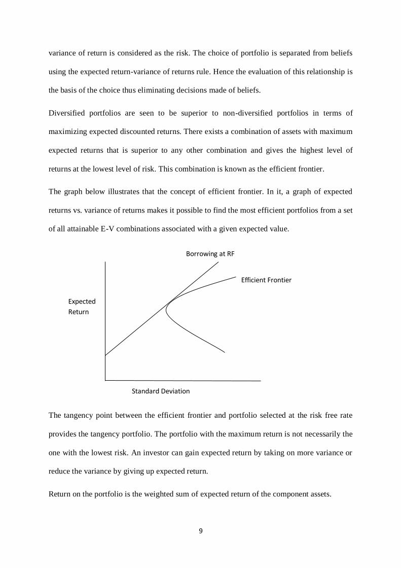
The graph below illustrates that the concept of efficient frontier. In it, a graph of expected

returns vs. variance of returns makes it possible to find the most efficient portfolios from a set

of all attainable E-V combinations associated with a given expected value.

The tangency point between the efficient frontier and portfolio selected at the risk free rate

provides the tangency portfolio. The portfolio with the maximum return is not necessarily the

one with the lowest risk. An investor can gain expected return by taking on more variance or

reduce the variance by giving up expected return.

Return on the portfolio is the weighted sum of expected return of the component assets.

Efficient Frontier

Expected

Return

Standard Deviation

Borrowing at RF

10

Where Rp is the return on the portfolio, Ri is the return on asset i and wi is the weighting of

component asset i (that is, the share of asset i in the portfolio).

Portfolio return variance is calculated as follows

Where ρij is the correlation coefficient between the returns on assets i and j. alternatively the

expression can be written as:

,

Where ρij = 1 for i=j.

The theory concludes that diversification provides a superior portfolio. It minimizes the

variance with caution being placed on ensuring that the assets don’t have a high covariance

with each other.

Weaknesses in the portfolio theory emerge from the difficulty in estimating the correlation

coefficient for two assets. It is even hard for multiple assets which require complex tools thus

it is not practical. In reality an almost unlimited range of possibilities of investment exist.

2.2.2 Capital Asset Pricing Model

The Capital Asset Pricing Model was first developed by William Sharpe (1964) and John

Lintner (1965). Sharpe and Lintner version of CAPM was based on the one period mean

variance portfolio theory of Markowitz. The Markowitz assumes that investors are risk

adverse and only care about risk (variance) and return (mean) of the asset’s one period

11

investment return. Therefore investors chose mean variance –efficient portfolio, meaning that

they either maximize the expected return, giving a certain variance of portfolio return or

minimize the variance given a certain expected return.

To obtain the CAPM in the basic form some assumptions need be fulfilled. Investors are

assumed to be risk adverse as in Markowitz Model and evaluate their investment only in

terms of excepted return and variance of return measure over the same single holding period.

Secondly, capital market are assumed to be perfect meaning that all assets are indefinitely

divisible, that no transactions cost, short selling restrictions or taxes occurs, that all investors

can lend and borrow at the risk free rate and that all information is costless and available for

everyone.

Thirdly, all investors have the same investment opportunities. Finally, all investors estimate

the same individual asset return, correlation amongst assets and standard deviation of return.

Based on these assumptions Sharpe and Lintner developed the following model

E(Ri)=Rf – βi (E(Rm)-Rf)

where

E(Ri) is the expected return of the asset

Rf is the risk-free rate

Βi is the beta

E(RM) is the expected return of the market

The expected return on assets E(Ri), is the risk-free rate (Rf), plus a premium per unit of beta

risk, which is calculated by subtracting the risk-free rate from the expected return of the

market, E(RM) and multiplying the result with the risk premium in terms of the asset’s

market beta, βiM.

12

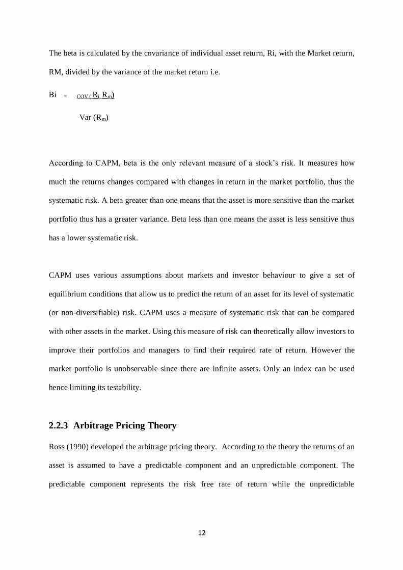
The beta is calculated by the covariance of individual asset return, Ri, with the Market return,

RM, divided by the variance of the market return i.e.

Βi = COV ( Ri, Rm)

Var (Rm)

According to CAPM, beta is the only relevant measure of a stock’s risk. It measures how

much the returns changes compared with changes in return in the market portfolio, thus the

systematic risk. A beta greater than one means that the asset is more sensitive than the market

portfolio thus has a greater variance. Beta less than one means the asset is less sensitive thus

has a lower systematic risk.

CAPM uses various assumptions about markets and investor behaviour to give a set of

equilibrium conditions that allow us to predict the return of an asset for its level of systematic

(or non-diversifiable) risk. CAPM uses a measure of systematic risk that can be compared

with other assets in the market. Using this measure of risk can theoretically allow investors to

improve their portfolios and managers to find their required rate of return. However the

market portfolio is unobservable since there are infinite assets. Only an index can be used

hence limiting its testability.

2.2.3 Arbitrage Pricing Theory

Ross (1990) developed the arbitrage pricing theory. According to the theory the returns of an

asset is assumed to have a predictable component and an unpredictable component. The

predictable component represents the risk free rate of return while the unpredictable

13

component is the risk based return. The fundamental logic of the APT is that investors will

engage in arbitrage where differences in return of assets with similar risk characteristics exist.

APT infers that investors are therefore only rewarded for assuming non-diversifiable risk.

The unpredictable component of returns to an asset will depend on macroeconomic factors

and industry-specific factors. Diversification will eliminate risk due to industry specific

factors hence only macro-economic factors will affect the expected risk premium. The

CAPM is largely a one factor model considering the sensitivity of an asset’s returns to market

returns changes as reflected in the asset beta. The APT assumes that the market risk is caused

by economic factors such as changes in the gross domestic product, inflation, and the

structure of the interest rate.

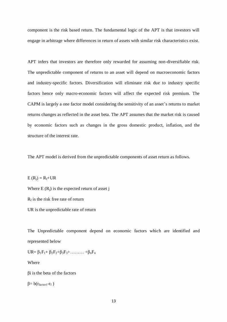
The APT model is derived from the unpredictable components of asset return as follows.

E (Rj) = Rf+UR

Where E (Rj) is the expected return of asset j

Rf is the risk free rate of return

UR is the unpredictable rate of return

The Unpredictable component depend on economic factors which are identified and

represented below

UR= β1F1+ β2F2+β3F3+……… +βnFn

Where

βi is the beta of the factors

β= b(rfactor1-rf )

14

The beta measures the sensitivity of each stock to the factor.

(rfactor1-rf ) estimates the risk premium on each factor. This is the difference between the

factors rate of return and the risk free rate of return.

Hence

E (Rj) = Rf + β1F1+β2F2+β3F3+……… +βnFn

The APT doesn’t require the market portfolio to be measured and can be used when only data

from a sample of risky assets is available. However the different factors are not defined in

this theory.

2.2.4 Fama-French Three –Factor Model

Fama and French developed the multifactor asset pricing model by identifying three factors

that affect a company’s profitability. It identifies two risk factors that are not considered in

the CAPM. The new factors include the size of the company and the book-to-market price

factor. These two factors together with the market risk premium factor form the three factor

model.

The company’s size significantly affects the rate of return of a company. Fama and French

found that stocks with a smaller market capitalization tended to do better than the market as a

whole. Hence the first factor is analysed by evaluating the difference between the returns of

small companies by market capitalization and the returns of big companies by market

capitalization. This forms the small minus big (SMB) factor. The sensitivity of the portfolio’s

return to this factor is then calculated in this model.

15

The second factor is the book-to-market price factor. Companies with a high book-to-market

value ratio are observed to do better than the market. Hence the second factor is computed by

calculating the high (book-to-market ratio) company returns minus low (book-to-market

ratio) company returns. This forms the ‘high minus low’ (HMS) factor. The third factor is the

market sensitivity ratio as define in CAPM as the difference between the asset return and the

market return.

The Fama and French model hence incorporates these three factors in the model below:

r = Rf + β3 (Km- Rf) + bs (SMB) + bv (HML) + €

where:

r is the portfolio or asset expected return

Rf risk-free rate of return

β3 is the beta factor of market return

Km is the market rate of return

bs is the coefficient of the SMB factor

SMB is the Small minus Big (market capitalization) factor

bv is the coefficient of the HML factor

HML is the high minus low (book-to-market ratio) factor

The bs and bv coefficient are determined by linear regression. The fama and French model

explains over 90% of the diversified portfolio’s returns which is higher than CAPM which

explains 70%.

16

2.3 Review of Empirical Theories

Gaumnitz (1970) evaluated the portfolio return variability and market price. He concluded

that portfolio managers are better off maximising the portfolio market prize to maximise

returns rather than try to minimise its variability. The returns on a portfolio vary more

significantly than the portfolio market price. Hence, the return measures dominated the risk

measures in calculation of the market price of risk than consideration of the variability.

Black, Jensen and Scholes (1972) improved the precision of the CAPM in estimating the beta

by working with portfolios rather than individual assets. The evaluation was not purely for

the pricing of a single asset but the pricing of a portfolio of assets. Jensen (1968) highlighted

the fact that a time-series regression test would prove the accuracy of the capital asset pricing

model. His evaluation considered the CAPM parameters and their estimation concluding that

a regression analysis would provide the estimate which would be used in the model. Actual

returns would then be compared with forecasts generated from the model. Significance test

proved that the beta was significant in explaining changes in explaining changes in expected

returns and estimates were within close range to the actual returns earned.

Portfolio risk is determined by the individual risk variances and the covariance with other

securities. Sears and Trennopohl (1993) indicated that the correlation is weighted by the

value of each asset to obtain the portfolio risk. A negative or positive correlation should be

used to add respective assets that minimise the level of risk of the whole portfolio.

Pogue (1974) observed that most investors are risk averse and will maximise their level of

expected return while minimising the level of risk in their investment. Bowman (1980)

however took exception where he noted a negative relationship between risk and returns.

17

This however occurred in cases where risk aversion was low such as in cases of troubled

firms. Such cases are driven by more long run expectation in turnaround of the troubled

firms.

Brigham, Gapenski & Davies (1999) found that the lower the coefficient of variation the

lower the risk per unit of return. Risk can be analysed using the coefficient of variation. This

is a relative measure of dispersion which measures the risk per unit of return. It is used to

compare assets that have different risk return characteristics.

Fletcher (1997) tested the conditional cross-sectional relationship between beta and portfolio

risk premiums in the UK stock market. He used the 30-day T-Bill rate as the risk-free rate

and the return on financial times all share index as the market portfolio. He found a positive

relationship between beta and portfolio risk premiums in the periods of up-market and a

negative relationship in the periods of low-market.

Elsas, El-shaer, and Theissen (2003) evaluated the beta-return relationship in the German

stock exchange. They tested the capital asset pricing model and its fundamental applicability

in the results of the stock exchange. The study did not find a significant relationship between

beta and risk but conditional test for individual industries found a significant posit ive

relationship.

Cresson (2002) used the correlation coefficient R2

as the market-based measure of portfolio

and mutual funds diversification. He found evidence that diversified portfolios and

diversified mutual funds have a significantly higher R than undiversified portfolios and

undiversified mutual funds respectively. With the complexities of portfolio theory and the

18

varied educational background of stockholders, an unambiguous, objective and easily

calculated measure of diversification such as R is of great value. He argued that R from the

market model regression is an important and valid measure of diversification.

Roll (1997) however heavily criticised the Capital asset pricing model due to the fact that the

market portfolio was unidentifiable. A market portfolio would include all risky assets

available in the market and would be infinite. He was in support of the arbitrage pricing

theory that evaluated more factors and included economic risk factors. This multifactor

model was derived by Ross (1990). In this theory the level of risk in an asset and therefore its

average expected return is directly related to anticipate changes in economic variables. These

factors include inflation, industrial productivity, risk premiums, slope of the term structure of

interest rates among others.

O’Neal (1997) researched on how many mutual funds constitute a diversified mutual fund

portfolio. Using simulation analysis he found that time-series diversification benefits are

minimal but the expected dispersion in terminal-period wealth can be substantially reduced

by holding multiple funds. Portfolios with as few as four growth funds halve the dispersion in

terminal-period wealth for 5 to 19-year holding periods. In addition, downside risk measures

decline as funds are added to portfolios. These advantages to multiple-fund portfolios are

especially meaningful for investors funding fixed-horizon investment goals such as

retirement or college savings.

Qi (2003) evaluated liquidity provision, interest-rate risk and the choice between banks and

mutual funds. He found that bank monitoring weakens lending rate constraints and thereby

leads to improved risk sharing and enhanced interim investment. All other factors constant,

high level of consumer liquidity needs and risk aversion, high levels of interest rates and

19

interest-rate variability, and low costs of bank monitoring favour the choice of banks over

mutual funds.

Cai, Chan & Yamadi (1997) analysed the performance of Japanese open type stock mutual

funds for the 1981-1992 period. The results show that, regardless of the performance

measures the benchmark employed, most of the japans mutual funds underperform the

benchmarks by between 3.6% and 10.8% per annum. These funds tend to invest more in large

stocks with low book-to-market ratios. But this feature does not explain the

underperformance. A potential explanation is the dilution effect caused by inflows of funds.

In japan, a new investor of an open-type fund only pays in the after-tax value of the net asset

value. They then conduct a bootstrap experiment to assess the magnitude of this dilution

effect and found it significantly high.

Saraoglu & Detzler (2002) evaluated a sensible mutual fund selection model. They presented

a rigorous framework for asset allocation; selecting mutual funds that take into account the

unique preferences and constraints of an individual investor. The framework is based on the

analytical hierarchy process (AHP) and the model generates reasonable asset-allocation

recommendations and identifies the most suitable funds within an asset class. They concluded

that a mutual funds selection model that uses the AHP framework is flexible, user friendly,

and ensures consistency throughout the portfolio decision process.

Fung & Hsieh (2002) analysed the asset-based style factors for hedge funds. The asset-based

style factors link returns of hedge funds strategies to observed market prices. They provide

explicit and unambiguous descriptions of hedge fund strategies that reveal the nature and

quantity of risk. Asset-based style factors are key inputs for portfolio construction and for

benchmarking hedge fund performance on a risk-adjusted basis. They used previously

20

developed models to construct asset-based style factors and demonstrate that one model

correctly predicted the return behaviour of trend-following strategies during out-of-sample

periods, in particular, during stressful market conditions like those of September 2001.

Comer (2006) examined the stock market timing ability of two samples of hybrid mutual

funds. He found that the inclusion of bonds indices’ and a bond timing variable in a

multifactor Treynor-Mzuy model framework leads to substantially different conclusions

concerning the stock market timing performance of these funds relative to the traditional

Treynor-Mazuy model. Results from this multifactor model find less stock timing ability over

the 1981-91 time periods and provide evidence of significant stock timing ability across the

second fund sample during the 1992-2000 time periods.

Babcork (1980) defined returns as the difference between investment value in the beginning

and end of the period, plus any cash flows received within the investment period. Modigliani

F and Pogue (1974) defined the rate of return as rate at which investor wealth increases and

decreases. Expected return is the weighted average of all possible outcomes. The expected

return can then be compared with the actual return post ante.

Taylor & Yoder (1994) investigated whether mutual fund trading activity by managers of

high-risk mutual funds make a positive contribution to investor utility. Stochastic dominance

is used to compare the returns of high-turnover funds with those of low-turnover funds. This

approach avoids the limitations of a mean/variance or regression approach and minimizes

problems of survivorship bias. The results show that high-turnover groups dominate low-

turnover groups, or at least are equally attractive to risk-averse investors. Active portfolio

management can enhance investor utility, even when the cost of obtaining and exploiting

costly information are taken into account.

21

Khorana & Servaes (1999) evaluated the determinants of mutual funds starts. Using a sample

of 1163 mutual funds started over the period 1979-1992, they found that fund initiations are

positively related to the level of assets invested in and the capital gains embedded in other

funds with the same objective, the fund family’s prior performance, the fraction of funds in

the family in the lower range fees, and the decision by large families to open similar funds in

the prior year. In addition, consistent with the presence of scale and scope economies in fund

openings, they found that large families and families that have more experience in opening

funds in the past are more likely to open new funds.

Bollen & Busse (2005) studied the short-term persistence in mutual fund performance. They

estimated parameters of standard stock selection and market timing models using daily

mutual fund returns and quarterly measurement periods. Ranking funds quarterly by

abnormal returns they measured the performance of each decile the following quarter. The

average abnormal return of the top decile in the post-ranking quarter was set at 39 basis

points. The post-ranking abnormal return disappears when funds are evaluated over longer

periods. These results suggested that superior performance is a short-lived phenomenon that

is observable only when funds are evaluated several times a year.

Indro, Jiang, Hu & Lee (1999) evaluated whether fund size affects a mutual fund’s

performance. They found that the fund size, which is the value of net assets under

management, affects the mutual funds’ performance. Mutual funds must attain a minimum

fund size in order to achieve sufficient returns to justify their costs of acquiring and trading

on information. Furthermore, there are diminishing marginal returns to information

acquisition and trading, and the marginal returns become negative when the mutual fund

22

exceeds its optimal size. In a sample of 683 non-indexed American equity funds over the

1993-95 periods, they found that 20 per cent of the mutual funds were smaller than the

breakeven-cost fund size and 10 per cent of the largest funds overinvested in information

acquisition and trading. In addition, they found that value funds and blend (value-and-

growth) funds have more to gain than growth funds from these information activities.

Grinblatt & Titman (1989) analysed mutual fund performance using quarterly portfolio

holdings. They employed the 1975-85 quarterly holdings of a sample of mutual funds to

construct an estimate of their gross returns. The sample which was not subject to survivor-

ship bias was used in conjunction with a sample that contains the actual (net) returns of the

mutual funds. In addition to allowing estimation of the bias in measured performance that is

due to the survival requirement it also afforded estimates of total transaction costs, and the

sample was used to test for existence of abnormal performance. The test indicated that the

risk-adjusted gross returns of some funds were significantly positive.

Arteaga, Ciccotello & Grant (1998) studied introduction of new equity funds, their marketing

and performance. They evaluate two strategies that sponsors have used successfully to

introduce new equity funds and promote the performance of the funds after their introduction.

The strategy of ‘incubation’ allows funds that reflect a favourable track record in the private

market to be marketed to the public at a later opportune time. The strategy of ‘selective

attention’ directs favourable allocations of ‘special situations’ into new funds that are open to

the public. Introduction strategies are most apparent among aggressive growth funds, where

first-year performance has increasingly become superior. Incubator funds remain small while

private, but once opened they quickly increase in size and revert to median performance. The

23

first-year success of selective attention funds also attracts large amount of cash, which

undermines their subsequent performance.

Ngene (2002) investigated the portfolio performance measures used by pension managers and

the challenges they face in portfolio management in Kenya. He established that most

investment managers are aware of the portfolio performance measures yet only one of the

nine respondents used the measures in pension fund management.

Maina (2003) researched on the risk and return of the investments held by insurance

companies in Kenya from January 1997 to December 2001. He concluded that there is very

little correlation between return and risk of investment held by Kenyan insurance companies.

Investment in secured loans however had a positive relationship between risk and returns.

Mutua, (2010) evaluated the relationship between portfolio composition, risk and return

among fund management firms in Kenya. He concluded that asset selection affects the risk

and return associated with a portfolio. He found that portfolio composition was widely

evaluated by fund managers in determining acceptable risk and achievable returns by the

fund.

2.4 Conclusion from Literature Review

A Portfolio is a combination of assets and securities held in an investment. Modigliani (1974)

indicates that investors attempt to maximise their portfolio returns within a given acceptable

level of portfolio risk. A portfolio allows for diversification to eliminate systematic risk and

goes further to reduce the overall level of portfolio risk. An optimal portfolio is the one that

offers the highest possible return for a specific level of risk or offers the lowest level of risk

for a given level of return. A portfolio may consist of both risk free assets and risky assets.

24

The literature review indicates that portfolio management has developed over the years

through various models that define the relationship between risk and returns. Empirical

research has tested the applicability of these models in actual portfolio management. In

Kenya the risk return relationship has been evaluated in the mutual funds market but none of

the studies has adopted the arbitrage pricing model. From the literature review we can

conclude that a research gap exists in testing the applicability of the arbitrage pricing model

in determining the risk return relationship in Kenyan mutual funds market.

25

CHAPTER THREE

3.0 RESEARCH METHODOLOGY

3.1 Research Design

This research project is a descriptive survey that determines the relationship between

variables and uses inferential statistics to derive conclusions. Descriptive survey according to

Mugenda and Mugenda (1999) describes relationships by collecting data from a population

and describe existing phenomena. Large data populations can be quantitatively analysed

using descriptive and inferential statistics.

3.2 Population

The target population for this study included sixteen registered fund managers registered by

the capital market authority. Only eleven of these fund managers operate mutual funds. They

operate a range of mutual funds with some operating more funds than others. This is the

entire group of agents constituting the mutual fund market in Kenya. Their characteristics

provided variables for the relationship between returns and the economic factors prevalent in

the market.

3.3 Sample Design

The population of eleven mutual fund managers provided a sample of seven fund managers

who operated funds for a period of four years that the study covered. Each fund manager

operates multiple funds hence a total of twenty three mutual funds were sampled for the

period between 2006 and 2012. A few of the funds operated for the period of seven years

with the shortest fund period sampled operating for four years. This ensured that the funds

could be comparatively reviewed thus funds operating for less than this minimum period

were not sampled.

26

3.4 Data Collection

This study used both primary and secondary data to test the relationship between the key

variables. Primary data was collected using a data form that individual mutual funds used to

fill their annual returns and fund size. The university introduction letter and a sample data

form are illustrated on Appendix 1. Published financial statements from three fund managers

provided secondary data for twelve mutual funds while primary data was collected from four

managers providing data on eleven mutual funds.

Secondary data was also obtained from officially published statistical data on national

statistics such as GDP growth rate, inflation rate and interest rates for the seven years period

between 2006 and 2012. Sources include the economic survey, World Bank online database,

African development bank database among others.

3.5 Data Analysis

This study analysed the arbitrage pricing model which consists of an arithmetic function of

returns as a function of economic variables. The study identified critical factors determining

the returns of mutual funds. It then measured the magnitude and significance of these factors.

Parameters for the independent factors were analysed to give inference to what really

influences returns and therefore the most critical factors in fund management.

The study analysed the time series variation in returns in the mutual fund market against

factors that constitute risk. It utilized the arbitrage pricing theory model by considering

unanticipated changes in economic factors which included the gross domestic product,

inflation, and interest rates. The level of risk premium in an asset and therefore its average

expected return is directly related to the anticipated changes in economic variables that affect

27

it. These factors include economic growth rate, inflation rate, interest rates, and the error

term. The fund size was also considered as a factor derived from the fund industry

specifically and that varies with each fund thus depicting intrinsic risk in each fund. The

model below was used:

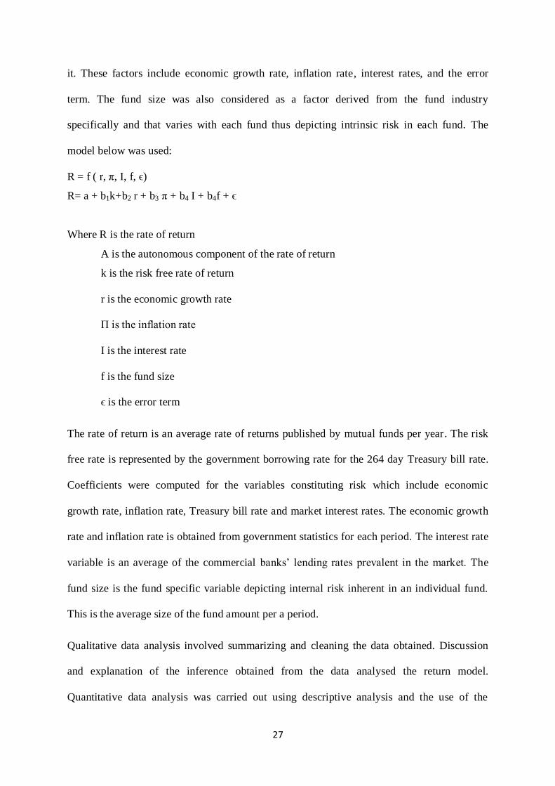
R = f ( r, π, I, f, ϵ)

R= a + b1k+b2 r + b3 π + b4 I + b4f + ϵ

Where R is the rate of return

A is the autonomous component of the rate of return

k is the risk free rate of return

r is the economic growth rate

Π is the inflation rate

I is the interest rate

f is the fund size

ϵ is the error term

The rate of return is an average rate of returns published by mutual funds per year. The risk

free rate is represented by the government borrowing rate for the 264 day Treasury bill rate.

Coefficients were computed for the variables constituting risk which include economic

growth rate, inflation rate, Treasury bill rate and market interest rates. The economic growth

rate and inflation rate is obtained from government statistics for each period. The interest rate

variable is an average of the commercial banks’ lending rates prevalent in the market. The

fund size is the fund specific variable depicting internal risk inherent in an individual fund.

This is the average size of the fund amount per a period.

Qualitative data analysis involved summarizing and cleaning the data obtained. Discussion

and explanation of the inference obtained from the data analysed the return model.

Quantitative data analysis was carried out using descriptive analysis and the use of the

28

statistical package for social sciences (SPSS). The model estimated the parameters that define

the correlation between the independent and the dependent variables. This model also

determined the magnitude of changes in the rate of return that can be explained by changes in

economic variables that influence risk.

29

CHAPTER FOUR

DATA ANALYSIS AND PRESENTATION

4.1 Introduction

Primary and secondary data collected for the dependent and independent variables is analysed

to determine the magnitude of parameters determining their relationship. The first section of

this chapter presents the data, explains the methods used to collect the data and the method

used to analyse the data. The second part explains the findings from the data analysis.

4.2 Data Presentation

4.2.1 Rate of return

The rate of return of mutual funds is the dependent variable in the analysis model with the

average rate of return being collected for each mutual fund. Data for the rates of return for a

period of seven years was collected. Some funds have only operated for four years from 2009

to 2012. The rate of return in published statements is the gross return before management fees

are charged and the net remitted to the investors. This rate of return represents the return on

the fund that is dependent on economic variables and investment decisions by the fund

managers. The average returns for balanced funds are the highest compared to other funds but

also represent greater volatility. They range from a high of 60.4% to a low of -39%. The

equity fund also depicts high return with high volatility. The money market on the other hand

has a relatively lower rate of return but with lower volatility. The average rate of returns has

changed over the seven years and the model analysis its relationship with the independent

variables. The average rates of returns are illustrated in appendix 1.

30

4.2.2 Treasury bill rate

The 182 day Treasury bill rate represents the risk free rate of government borrowing. An

average of this rate was obtained per year for the period of seven years. The highest rate was

13.54% in 2012 and the lowest rate being 3.81% in 2010. The majority on treasury rates lie

between 7% and 8% with an average rate of 8.36%. Money market and balanced funds by

definition have investments in treasury bills. The mutual funds market performance is

influenced by the Treasury bill rate since the rate is used by the fund managers as the base

line rate. The Treasury bill rates for the period are illustrated in appendix 2.

4.2.3 GDP growth rate

The GDP growth rate indicates the changes in the economic and is the main indicator or

expansion or recession. It is therefore a key indicator of the economic risk prevalent in an

economy affecting the returns to mutual funds and other investments. Secondary data on the

GDP growth rate was collected from the economic survey and African development bank

online database. The highest GDP growth rate was recorded in 2007 at 6.99% and the lowest

in 2008 at a rate 1.53%. The average growth rate for the period is 4.56% and a median of

4.38%. The GDP growth rates for the period are illustrated in appendix 2.

4.2.4 Inflation rate

Data on the annual inflation rate for the period of seven years from 2006 to 2012 was

collected for the second independent variable in the model. The inflation rate reduces the real

returns to the investor as the time value money diminishes. Investors adjust their expected

rate of return depending on the prevailing inflation rate. The highest inflation rate for the

period was at 16.20% in 2008 and the lowest rate at 4.08% in 2010. The median inflation rate

is 9.65 with an average rate of 9.25%. This data was collected from secondary sources

31

including the economic survey and the African development bank online database. The

inflation rates are illustrated in appendix 2.

4.2.5 Market Interest rates

The market interest rate represents the average lending rate offered by commercial banks.

Data was collected on the average market interest rates per year for the seven years period.

The secondary data was obtained from the World Bank and the central bank online databases.

Market interest rates represent the cost of financing and hence affect the rate of returns. The

highest market interest rate for the period was at 19.63% in 2012 and lowest in 13.30% in

2007. The average rate for the period is at 14.96 with a median of 14.40. The market interest

rates are illustrated in appendix 2.

4.2.6 Fund size

The size of the fund represents an internal factor that is unique to each fund. It therefore

illustrates the internal risk inherent in the fund since it changes from year to year. Data on

mutual fund size was collected from both primary and secondary sources. Published financial

statements were available for twelve funds while a data form was used to collect primary data

from eleven funds. The fund size is the fifth independent variable in the model representing

the risk return relationship whose beta parameter is analysed. The equity fund has the biggest

fund size with the old mutual equity fund of 5.8 billion shillings in 2007. Money market fund

follows in fund size with the balanced fund and bond fund following the rank. The fund size

generally rises with time hence funds that have existed for a long time are bigger. This

variable helped determine whether fund size affects the rate of return and how much inherent

risk it represents. The mutual fund sizes are illustrated in appendix 1.

32

4.3 Model Analysis

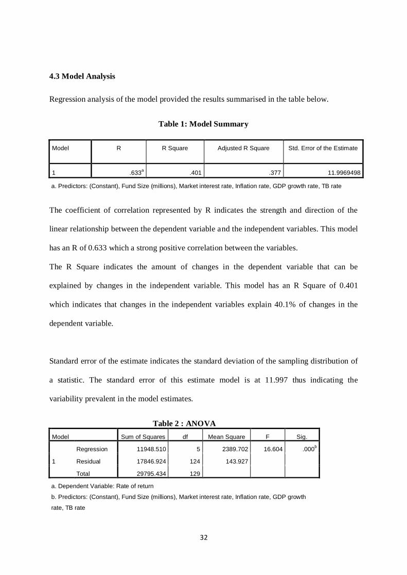
Regression analysis of the model provided the results summarised in the table below.

Table 1: Model Summary

Model R R Square Adjusted R Square Std. Error of the Estimate

1 .633a .401 .377 11.9969498

a. Predictors: (Constant), Fund Size (millions), Market interest rate, Inflation rate, GDP growth rate, TB rate

The coefficient of correlation represented by R indicates the strength and direction of the

linear relationship between the dependent variable and the independent variables. This model

has an R of 0.633 which a strong positive correlation between the variables.

The R Square indicates the amount of changes in the dependent variable that can be

explained by changes in the independent variable. This model has an R Square of 0.401

which indicates that changes in the independent variables explain 40.1% of changes in the

dependent variable.

Standard error of the estimate indicates the standard deviation of the sampling distribution of

a statistic. The standard error of this estimate model is at 11.997 thus indicating the

variability prevalent in the model estimates.

Table 2 : ANOVA

Model Sum of Squares df Mean Square F Sig.

1

Regression 11948.510 5 2389.702 16.604 .000b

Residual 17846.924 124 143.927

Total 29795.434 129

a. Dependent Variable: Rate of return

b. Predictors: (Constant), Fund Size (millions), Market interest rate, Inflation rate, GDP growth

rate, TB rate

33

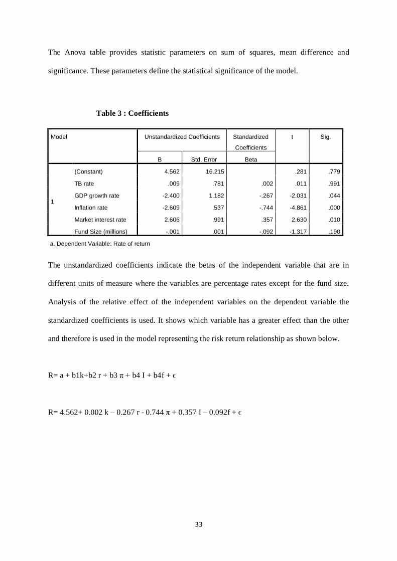
The Anova table provides statistic parameters on sum of squares, mean difference and

significance. These parameters define the statistical significance of the model.

Table 3 : Coefficients

Model Unstandardized Coefficients Standardized

Coefficients

t Sig.

B Std. Error Beta

1

(Constant) 4.562 16.215 .281 .779

TB rate .009 .781 .002 .011 .991

GDP growth rate -2.400 1.182 -.267 -2.031 .044

Inflation rate -2.609 .537 -.744 -4.861 .000

Market interest rate 2.606 .991 .357 2.630 .010

Fund Size (millions) -.001 .001 -.092 -1.317 .190

a. Dependent Variable: Rate of return

The unstandardized coefficients indicate the betas of the independent variable that are in

different units of measure where the variables are percentage rates except for the fund size.

Analysis of the relative effect of the independent variables on the dependent variable the

standardized coefficients is used. It shows which variable has a greater effect than the other

and therefore is used in the model representing the risk return relationship as shown below.

R= a + b1k+b2 r + b3 π + b4 I + b4f + ϵ

R= 4.562+ 0.002 k – 0.267 r - 0.744 π + 0.357 I – 0.092f + ϵ

34

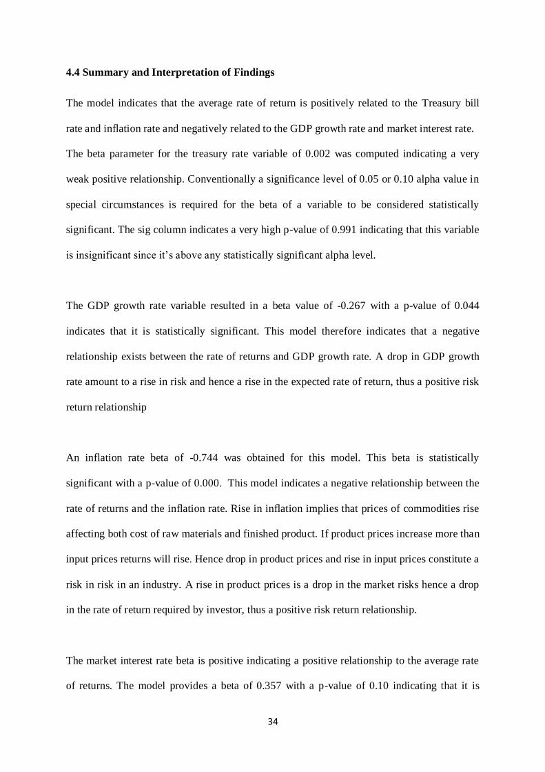
4.4 Summary and Interpretation of Findings

The model indicates that the average rate of return is positively related to the Treasury bill

rate and inflation rate and negatively related to the GDP growth rate and market interest rate.

The beta parameter for the treasury rate variable of 0.002 was computed indicating a very

weak positive relationship. Conventionally a significance level of 0.05 or 0.10 alpha value in

special circumstances is required for the beta of a variable to be considered statistically

significant. The sig column indicates a very high p-value of 0.991 indicating that this variable

is insignificant since it’s above any statistically significant alpha level.

The GDP growth rate variable resulted in a beta value of -0.267 with a p-value of 0.044

indicates that it is statistically significant. This model therefore indicates that a negative

relationship exists between the rate of returns and GDP growth rate. A drop in GDP growth

rate amount to a rise in risk and hence a rise in the expected rate of return, thus a positive risk

return relationship

An inflation rate beta of -0.744 was obtained for this model. This beta is statistically

significant with a p-value of 0.000. This model indicates a negative relationship between the

rate of returns and the inflation rate. Rise in inflation implies that prices of commodities rise

affecting both cost of raw materials and finished product. If product prices increase more than

input prices returns will rise. Hence drop in product prices and rise in input prices constitute a

risk in risk in an industry. A rise in product prices is a drop in the market risks hence a drop

in the rate of return required by investor, thus a positive risk return relationship.

The market interest rate beta is positive indicating a positive relationship to the average rate

of returns. The model provides a beta of 0.357 with a p-value of 0.10 indicating that it is

35

statistically significant. An increase in market interest rates implies that the cost of borrowing

has increased in the risk to mutual funds returns. This indicates a positive a positive risk

return relationship.

A negative beta for the fund size parameter indicates a negative relationship with the average

rate of return. A beta of -0.092 with a p-value of 0.19 indicates that it is statistically

significant but with a low level of level of significance. This indicates that the smaller the

fund size the higher the inherent risk hence investors will demand a higher rate of return.

Muriithi (2005) found a positive relationship between risk and returns in the mutual funds

market in Kenya for the period between 2003 and 2005. This study obtained similar results

using the arbitrage pricing model for the period between 2006 and 2012.

Maina (2003) found insignificant relationship between risk and return in investments held by

insurance companies in Kenya from January 1997 to December 2001. Mutua (2010) found a

positive relationship in between portfolio composition, risk and return among fund

management firms in Kenya. This study finds a significant positive relationship between risk

and return as per the economic variables analysed. It therefore reinforces the positive

relationship observed by Mutua (2010) and Muriithi (2005) in this case evaluating different

variables with unique magnitude on changes in returns.

36

CHAPTER FIVE

SUMMARY, CONCLUSIONS AND RECOMMENDATIONS

5.1 Summary

The main objective of this research study was to analyse the beta parameters of factors that

define the risk return relationship in the Kenyan mutual funds market using the arbitrage

pricing model. A descriptive research design was used to collect and analyse data which

involves observing and describing the relationship between variables. The arbitrage pricing

model was used to select economic variables that define risk in the mutual funds market. The

economic variables selected included the Treasury bill rate, GDP growth rate, inflation rate,

market interest rate and fund size.

Data was collected from various mutual funds managers operating different mutual funds.

The funds included the money market fund, equity fund, balanced fund, bond fund and

Kenya shillings fund. Both primary and secondary data was collected and analysed through

linear regression. The average rate of returns was observed to be negatively related to the

GDP growth rate, inflation rate and fund size.

A positive relationship was found in the relationship between average rate of returns and

market interest rates and the Treasury bill rate. The beta parameter for the GDP growth rate,

inflation rate and market interest rate are statistically significant. The beta parameter for the

Treasury bill rate was found to be statistically insignificant. These beta variables were found

to represent a positive relationship in the risk return relationship with unique magnitudes for

each factor. The market interest rates, GDP growth rate and inflation rate have the greatest

impact on rates of return. The fund size has slightly weaker but significant beta with the TB

rate being insignificant.

37

5.2 Conclusions

A negative beta which is statistically significant was obtained for the GDP growth rate. This

implies that a decrease in the economic growth rate is an increase in the risk faced by

investors hence they will demand a higher rate of return. The drop in the GDP growth rate

represents worsening of the economic condition. This leads to the conclusion that a positive

relationship exists in the risk return variables where the GDP growth rate variable is used to

evaluate the risk changes in an economy.

A statistically significant negative beta was obtained for the inflation rate variable in this

model. This implies that an increase in the price level results in a lower rate of returns to

mutual funds. Where inflation results in product prices rising higher than input prices a

higher return would be realized, as is the case in most Kenyan markets. Consequently a rise

in the inflation rate would be a drop in the market risks hence a drop in the rate of return

required by investor.

The market interest rate beta obtain is positive and statistically significant. This implies that

an increase in cost of borrowing is a risk faced by investors since it reduces their margins.

Hence when the market interest rate increase the investor will demand a higher rate of return

to cover the higher risk undertaken. A slightly weaker, statistically significant negative beta

for the fund size beta was obtained for this model. This implies that the smaller the fund size

the higher the inherent risk in a mutual fund. Therefore an investor will demand a higher rate

of return for the higher risk. The conclusion from this model is that a positive risk return

relationship exists in the mutual fund market agreeing with theory but with different impact

of variables on risk and returns.

38

5.3 Policy Recommendations

The conclusion made from this research study supports the following government and mutual

funds policy recommendation. The government should adopt expansionary economic policies

that ensure high GDP growth rate to ensure that returns in each sector increase and reduce the

risk prevalent in the economy. This will result in higher returns to the mutual funds since they

are invested in different sectors of the economy.

The central bank should control the base lending rate to commercial banks to control inflation

and also ensure appropriate cost of borrowing in the market. High inflation reduces the real

returns to mutual funds and other investments. Hence when the inflation rate is rising, the

base lending rate should be raised to reduce the money supply and reduce the purchasing

power. On the other hand the base lending rate to commercial bank should be regulated to

ensure that the cost of borrowing remains low enough to stimulate more investment and

better returns.

Mutual funds policies and business strategies should be tailored to address the factors that

determine the risks and returns in the market. Mutual fund managers should adopt

diversification policies to mitigate economic changes in different industries. Investing in

different industries that are negatively correlated eliminates systematic risk. The inflation

rate is less felt in some industries than others hence a diversified portfolio will achieve better

returns than undiversified ones.

A large fund size enjoys economies of scale and broader diversification option. This study

found that bigger funds earned higher returns than small ones. Effective marketing strategies

should be adopted to attract more investors and merging of smaller funds.

39

5.4 Limitations of the Study

When conducting this research study a number of limitations were encountered. The first

limitation was the assumptions made by under the arbitrage pricing model. The model

assumes that there are no transaction costs and taxes. Consequently the rate of returns is

computed before the management fees and taxes are deducted. However the actual return

received by the investor is the net returns. The factors affecting the rate of return will

influence the gross return achieved by the fund manager.

Another limitation was the existence of low informational efficiency in the mutual funds

market. The Nairobi exchange market has grown tremendously but still hasn’t achieved high

information efficiency where prices of an asset reflect all information available. Most mutual

funds invest in the stock market and also publish the rate of returns they offer on a daily

basis. However prices change with a lag effect as the economic variables change.

Another limitation is the possibility of different mutual funds being affected by the variable

factors by differently. The money market fund is affected by the treasury bill rate by a greater

magnitude than the balance fund. Similarly variables affecting the equity fund and Kenyan

shillings fund will be affected by the economic growth rate and inflation by different

magnitude.

Fourthly, the research is limited to data provided by mutual fund which conforms to period

financial reporting statements. This implies that the cut off of a period can be in the middle of

an economic cycle hence provides return statistics before the market corrects its self. This can

be observed in the data where the return could drop drastically for one year and rise

drastically the next year providing a normal average return for the two years.

40

5.5 Suggestions for Further Studies

Further studies relating to this research topic can be undertaken in the following areas.

Firstly, an analysis of the mutual funds market based on the CAPM model can determine the

performance of mutual funds relative to the market. Mutual funds managers attract investors

by promising a higher return than the market. An analysis comparing actual returns if an

investor held a market portfolio can be analysed using the CAPM to derive the premium

generated by mutual funds. This analysis would provide a view to analyse the risk return

relationship in the mutual funds market.

Secondly, further studies can analyse risk factors that are unique to sectors that individual

mutual funds are invested in. Bond funds, equity funds and Kenya shillings funds can be

affected with different magnitude by the economic factors analysed by the arbitrage pricing

model. Some funds may be highly influenced by a certain factor hence policies and business

strategies are unique to them.

Thirdly, the mutual funds market can also be analysed using the three factor model. This

pricing model would analyse the risk return relationship as represented by the three factors. A

beta parameter for the market factor, size factor and book to market factor indicates how

sensitive a portfolio is to changes in this ratio.

Fourthly, a comparative study on the performance of mutual funds relative to pension funds

and the factors that are unique to each of them can be analysed. Both funds invest in different

sectors but with different investment objectives. The marketing and investment strategies

differ resulting in risks and returns that are unique to each type of fund.

41

REFERENCES

Arteaga, K.R, Ciccotello, C.S, & Grant, C.T. (1998). New Equity Funds: Marketing and

Performance, Financial analysts Journal, 54(6), 43-49.

Black, Fischer (1972). Capital Market Equilibrium with Restricted Borrowing. Journal of

business, 45(3), 444-454.

Bollen, N.P.B. & Busse, J.A. (2005). Short-Term Persistence in Mutual Fund Performance.

The Review of financial Studies, 18(2), 569-597.

Browman E.H. (1980). A Risk Return Paradox for Strategic Management, Sloan

Management Review.

Comer, G. (2006). Hybrid Mutual Funds and Market Timing Performance. The Journal of

Business, 79(2), 771-797.

Cresson J.E. (2002). R2: A Market–based measure of portfolio and mutual fund

diversification. Quarterly Journal of Business and Economic, 41(3/4), 115-143.

Cai, J., Chan K.C & Yamadi, T. (1997). The Performance of Japanese Mutual Funds. The

Review of financial Studies, 10(2), 237-273.

Elsas, R., El-shaer, M. & Theissen, E. (2003) Beta and Return revisited: Evidence from the

German stock market. J ournal of International Financial Markets, Institutions and money,

13(1), 1-18.

42

Fama, E. & French, K. (1992). The cross-section of expected stock returns. Journal of

finance, 47, 427-465.

Fletcher, J. (1997). An examination of the cross-sectional relationship of beta and return; UK

evidence. Journal of economics and business, 49(3), 211-221.

Fung, W. & Hsieh, D.A. (2002) Asset-Based Style Factors for Hedge Funds. Financial

Analysts Journal, 58(5), 16-27.

Gaumnitz, J.E. (1970) Appraising Performance of Investment Portfolios. The Journal of

finance: The journal of the American Finance Association, 25(3), 555-560.

Grinblatt, M. & Titman,S. (1989) Mutual Fund Performance: An Analysis of Quartely

Portfolio Holdings. The Journal of Business, 62(3), 393-416.

Indro, D.C, Jiang, C.X, Hu, M.Y, & Lee, W.Y. (1999) Mutual Fund Performance: Does Fund

Size Matter? Financial Analysts Journal, 55(3), 74-87.

Jensen, M.C. (1972) Optimal Utilization of Market Forecast and evaluation of Investment

performance in G. P. Szego and K. shell (eds.) Mathematical Methods of Investment &

Finance, Amsterdam : North Holland.

Jensen, M.C. (1968) The Performance of Mutual Funds in the period 1945-1964. Journal of

Finance, 23(2), 389-416.

43

Khorana, A. & Servaes, H. (1999) The Determinants of Mutual Funds Starts. The review of

financial studies, 12(5), 1043-1074.

Markowitz (1952). Portfolio Selection. Journal of Finance, 7, 77-91.

Miller, Merton & Scholes, M. (1972). Rate of Return in Relation to Risk: A Re-examination

of some recent findings in studied in the theory of Capital Markets. Michael C. Jensen, eds

New York: Praeger, 47-75.

Muriithi D.K. (2005) An Evaluation of the Risk & Return of Equity Mutual Funds in Kenya,

Unpublished MBA Project, University of Nairobi.

Mutua, F.M. (2010) the relationship between portfolio composition and risk and return

among fund Management firms in Kenya, Unpublished MBA Project, University of Nairobi.

Ngene, G.M. (2002) Empirical Investigation into Portfolio Performance Measures by Pension

Fund Managers and the Challenges they face in Portfolio Management in Kenya,

Unpublished MBA Project, University of Nairobi.

O’Neal, E.S. (1997) How Many Mutual funds constitute a Diversified Mutual Fund

Portfolio? Financial Analysts Journal, 53(2), 37-46.

Ramsany, B.H. & Yeung M.C (2003) Evaluating Mutual Funds in an Emerging Market:

Factors that matter to financial advisors, International Journal of Bank marketing, 122- 136.

44

Roll, R. (1997) A Critique of the Asset Pricing Theory’s Tests Part 1: On Past and Potential

Testability of the Theory. Journal of Financial Economics, 4(2), 129-176.

Ross, S.A., Westefield, R.W., & Jaffe, F.J. (1990) Corporate Finance, 2nd Edition Irwin, 295-

311

Roy, S.M. (2005) Money Market Mutual Funds: A Macro Perspective, Economic and

Political weekly, 40(12) Mutual, Banking and Finance (Mar, 19-25, 2005), 1254-1256, 1258-

1263.

Taylor, W.R.L. & Yoder, J.A. (1994). Mutual Fund Trading and Investor Utility. Financial

analysts Journal, 50(3), 66-69.

Saraoglu, H. & Detzler M.L. (2002). A Sensible Mutual Funds Selection Model. Financial

Analysts Journal, 58(3), 60-72.

Sharpe, W.F. (1964). Capital Asset Prices: A Theory of Market Equilibrium under conditions

of Risk. Journal of Finance, 19(3), 425-442.

Qi, J. (2003). Liquidity Provision, Interest-Rate Risk, and the Choice between Banks and

Mutual funds, Journal of Institutional and Theoretical Economics, 159(3), 491-510.

45

APPENDICES

APPENDIX 1: Introduction letter

46

APPENDIX 2: Data collection Form

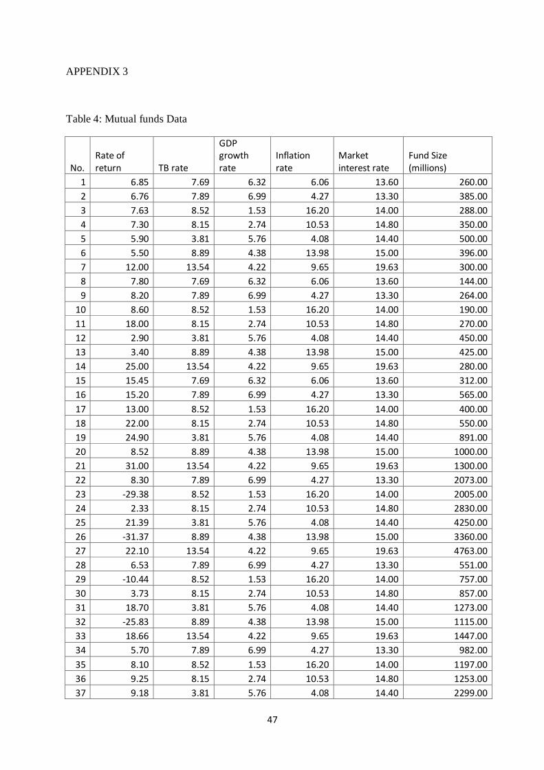
47

APPENDIX 3

Table 4: Mutual funds Data

No. Rate of return TB rate

GDP growth rate

Inflation rate

Market interest rate

Fund Size (millions)

1 6.85 7.69 6.32 6.06 13.60 260.00

2 6.76 7.89 6.99 4.27 13.30 385.00

3 7.63 8.52 1.53 16.20 14.00 288.00

4 7.30 8.15 2.74 10.53 14.80 350.00

5 5.90 3.81 5.76 4.08 14.40 500.00

6 5.50 8.89 4.38 13.98 15.00 396.00

7 12.00 13.54 4.22 9.65 19.63 300.00

8 7.80 7.69 6.32 6.06 13.60 144.00

9 8.20 7.89 6.99 4.27 13.30 264.00

10 8.60 8.52 1.53 16.20 14.00 190.00

11 18.00 8.15 2.74 10.53 14.80 270.00

12 2.90 3.81 5.76 4.08 14.40 450.00

13 3.40 8.89 4.38 13.98 15.00 425.00

14 25.00 13.54 4.22 9.65 19.63 280.00

15 15.45 7.69 6.32 6.06 13.60 312.00

16 15.20 7.89 6.99 4.27 13.30 565.00

17 13.00 8.52 1.53 16.20 14.00 400.00

18 22.00 8.15 2.74 10.53 14.80 550.00

19 24.90 3.81 5.76 4.08 14.40 891.00

20 8.52 8.89 4.38 13.98 15.00 1000.00

21 31.00 13.54 4.22 9.65 19.63 1300.00

22 8.30 7.89 6.99 4.27 13.30 2073.00

23 -29.38 8.52 1.53 16.20 14.00 2005.00

24 2.33 8.15 2.74 10.53 14.80 2830.00

25 21.39 3.81 5.76 4.08 14.40 4250.00

26 -31.37 8.89 4.38 13.98 15.00 3360.00

27 22.10 13.54 4.22 9.65 19.63 4763.00

28 6.53 7.89 6.99 4.27 13.30 551.00

29 -10.44 8.52 1.53 16.20 14.00 757.00

30 3.73 8.15 2.74 10.53 14.80 857.00

31 18.70 3.81 5.76 4.08 14.40 1273.00

32 -25.83 8.89 4.38 13.98 15.00 1115.00

33 18.66 13.54 4.22 9.65 19.63 1447.00

34 5.70 7.89 6.99 4.27 13.30 982.00

35 8.10 8.52 1.53 16.20 14.00 1197.00

36 9.25 8.15 2.74 10.53 14.80 1253.00

37 9.18 3.81 5.76 4.08 14.40 2299.00

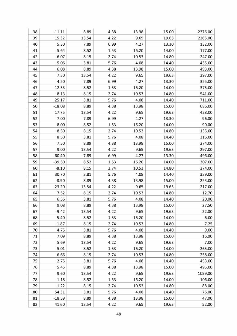
48

38 -11.11 8.89 4.38 13.98 15.00 2376.00

39 15.32 13.54 4.22 9.65 19.63 2265.00

40 5.30 7.89 6.99 4.27 13.30 132.00

41 5.64 8.52 1.53 16.20 14.00 177.00

42 6.07 8.15 2.74 10.53 14.80 247.00

43 5.06 3.81 5.76 4.08 14.40 435.00

44 6.08 8.89 4.38 13.98 15.00 493.00

45 7.30 13.54 4.22 9.65 19.63 397.00

46 4.50 7.89 6.99 4.27 13.30 355.00

47 -12.53 8.52 1.53 16.20 14.00 375.00

48 8.13 8.15 2.74 10.53 14.80 541.00

49 25.17 3.81 5.76 4.08 14.40 711.00

50 -18.08 8.89 4.38 13.98 15.00 686.00

51 17.75 13.54 4.22 9.65 19.63 428.00

52 7.00 7.89 6.99 4.27 13.30 96.00

53 8.00 8.52 1.53 16.20 14.00 90.00

54 8.50 8.15 2.74 10.53 14.80 135.00

55 8.50 3.81 5.76 4.08 14.40 316.00

56 7.50 8.89 4.38 13.98 15.00 274.00

57 9.00 13.54 4.22 9.65 19.63 297.00

58 60.40 7.89 6.99 4.27 13.30 496.00

59 -39.50 8.52 1.53 16.20 14.00 307.00

60 -8.10 8.15 2.74 10.53 14.80 274.00

61 30.70 3.81 5.76 4.08 14.40 339.00

62 -8.90 8.89 4.38 13.98 15.00 253.00

63 23.20 13.54 4.22 9.65 19.63 217.00

64 7.52 8.15 2.74 10.53 14.80 12.70

65 6.56 3.81 5.76 4.08 14.40 20.00

66 9.08 8.89 4.38 13.98 15.00 27.50

67 9.42 13.54 4.22 9.65 19.63 22.00

68 -5.40 8.52 1.53 16.20 14.00 6.00

69 -1.87 8.15 2.74 10.53 14.80 7.25

70 4.75 3.81 5.76 4.08 14.40 9.00

71 7.09 8.89 4.38 13.98 15.00 16.00

72 5.69 13.54 4.22 9.65 19.63 7.00

73 5.01 8.52 1.53 16.20 14.00 265.00

74 6.66 8.15 2.74 10.53 14.80 258.00

75 2.75 3.81 5.76 4.08 14.40 453.00

76 5.45 8.89 4.38 13.98 15.00 495.00

77 9.60 13.54 4.22 9.65 19.63 1059.00

78 1.18 8.52 1.53 16.20 14.00 106.00

79 1.22 8.15 2.74 10.53 14.80 88.00

80 54.31 3.81 5.76 4.08 14.40 76.00

81 -18.59 8.89 4.38 13.98 15.00 47.00

82 41.60 13.54 4.22 9.65 19.63 52.00

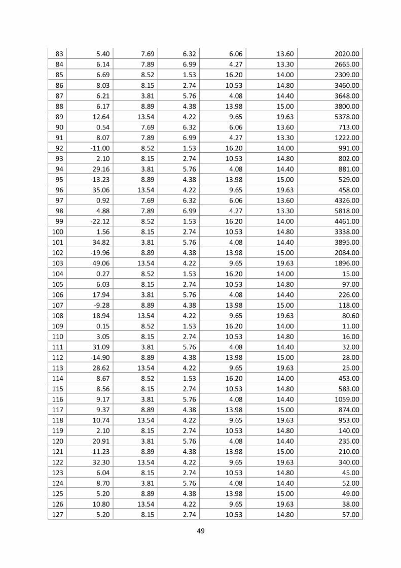
49

83 5.40 7.69 6.32 6.06 13.60 2020.00

84 6.14 7.89 6.99 4.27 13.30 2665.00

85 6.69 8.52 1.53 16.20 14.00 2309.00

86 8.03 8.15 2.74 10.53 14.80 3460.00

87 6.21 3.81 5.76 4.08 14.40 3648.00

88 6.17 8.89 4.38 13.98 15.00 3800.00

89 12.64 13.54 4.22 9.65 19.63 5378.00

90 0.54 7.69 6.32 6.06 13.60 713.00

91 8.07 7.89 6.99 4.27 13.30 1222.00

92 -11.00 8.52 1.53 16.20 14.00 991.00

93 2.10 8.15 2.74 10.53 14.80 802.00

94 29.16 3.81 5.76 4.08 14.40 881.00

95 -13.23 8.89 4.38 13.98 15.00 529.00

96 35.06 13.54 4.22 9.65 19.63 458.00

97 0.92 7.69 6.32 6.06 13.60 4326.00

98 4.88 7.89 6.99 4.27 13.30 5818.00

99 -22.12 8.52 1.53 16.20 14.00 4461.00

100 1.56 8.15 2.74 10.53 14.80 3338.00

101 34.82 3.81 5.76 4.08 14.40 3895.00

102 -19.96 8.89 4.38 13.98 15.00 2084.00

103 49.06 13.54 4.22 9.65 19.63 1896.00

104 0.27 8.52 1.53 16.20 14.00 15.00

105 6.03 8.15 2.74 10.53 14.80 97.00

106 17.94 3.81 5.76 4.08 14.40 226.00

107 -9.28 8.89 4.38 13.98 15.00 118.00

108 18.94 13.54 4.22 9.65 19.63 80.60

109 0.15 8.52 1.53 16.20 14.00 11.00

110 3.05 8.15 2.74 10.53 14.80 16.00

111 31.09 3.81 5.76 4.08 14.40 32.00

112 -14.90 8.89 4.38 13.98 15.00 28.00

113 28.62 13.54 4.22 9.65 19.63 25.00

114 8.67 8.52 1.53 16.20 14.00 453.00

115 8.56 8.15 2.74 10.53 14.80 583.00

116 9.17 3.81 5.76 4.08 14.40 1059.00

117 9.37 8.89 4.38 13.98 15.00 874.00

118 10.74 13.54 4.22 9.65 19.63 953.00

119 2.10 8.15 2.74 10.53 14.80 140.00

120 20.91 3.81 5.76 4.08 14.40 235.00

121 -11.23 8.89 4.38 13.98 15.00 210.00

122 32.30 13.54 4.22 9.65 19.63 340.00

123 6.04 8.15 2.74 10.53 14.80 45.00

124 8.70 3.81 5.76 4.08 14.40 52.00

125 5.20 8.89 4.38 13.98 15.00 49.00

126 10.80 13.54 4.22 9.65 19.63 38.00

127 5.20 8.15 2.74 10.53 14.80 57.00

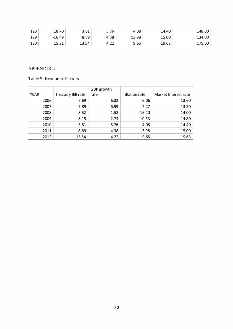
50

128 18.70 3.81 5.76 4.08 14.40 148.00

129 -16.49 8.89 4.38 13.98 15.00 134.00

130 15.31 13.54 4.22 9.65 19.63 175.00

APPENDIX 4

Table 5: Economic Factors

YEAR Treasury Bill rate GDP growth rate Inflation rate Market Interest rate

2006 7.69 6.32 6.06 13.60

2007 7.89 6.99 4.27 13.30

2008 8.52 1.53 16.20 14.00

2009 8.15 2.74 10.53 14.80

2010 3.81 5.76 4.08 14.40

2011 8.89 4.38 13.98 15.00

2012 13.54 4.22 9.65 19.63