A Study of Mutual Fund Flow and Market Return Volatility

Eric C. Chang

School of Business

The University of Hong Kong

Pokfulam Road, Hong Kong

Tel: (852) 2857-8347

Fax: (852) 2858-5614

Email: ecchang@business.hku.hk

and

Ying WANG

School of Business

The University of Hong Kong

Pokfulam Road, Hong Kong

Tel: (852) 2249-0615

Fax: (852) 2858-5614

Email: wypony@business.hku.hk

This Draft: May 17, 2002

Very Preliminary

For Conference Submission

2

A Study of Mutual Fund Flow and Market Return Volatility

Abstract

In this study, we investigate the impact of institutional trading on the market by

examining the daily relation between aggregate flow into U.S. equity funds and

market volatility. We differentiate the impact of fund inflow and outflow, respectively,

on the market volatility. Our empirical results show that there exists an asymmetric

concurrent relationship between fund flow and market volatility: fund inflow is

negatively correlated with market volatility while fund outflow is positively correlated

with market volatility. We also discuss the potential explanations for our results and

suggest that our results are consistent with information content differences of funds’

buys and sales.

3

1. Introduction

Stock market volatility has received great attention from investors, regulators, press

and academicians and is especially closely watched by many option traders since the

option value is largely dependent on the volatility of its underlying asset. Existing

literature documents evidence that volatility is time-varying and calls for a better

understanding why volatility has changed over time. For example, based on monthly

observations, Schwert (1989) reports that stock volatility exhibits substantial changes

from 1857 to 1987. Haugen, Talmor, and Torous (1991) document a large variation in

volatility over the period 1897 through 1988 by using daily return data. Lockwood

and Linn (1990) examine the intraday market returns during 1964-1989 and show that

volatility is higher for intraday than overnight periods.

The popular press often quotes the view of practitioners to suggest that greater

institutional participation may account for the volatility variation. Sias (1996), for

example, quotes “Reviewing this week’s events, analysts are concluding that

professional investors simply overreacted… ” (Wall Street Journal (WSJ), July 21,

1995, p. A1). The quote highlights that institutional traders have been perceived as a

contributor to the stock market volatility. This view is echoed by another quote:

“Small investors, through their purchase of stock mutual funds, have emerged as the

major driving force that has propelled the Dow Jones Industrial Average.” (WSJ,

February 26, 1993, p. C1).

Notwithstanding these perceptions and fears, we know little empirically about the

relationship between market volatility and institutional traders, especially the mutual

fund traders. Recently, considerable academic attention has been given to the price

impact of mutual fund trading. While many prior studies have documented the price

effect of money inflow into a mutual fund on individual mutual funds (Chan and

Lakonishok, 1993, 1995, 1997; Keim and Madhavan, 1997; Jones and Lipson, 1999),

some other literatures study the relation between the aggregate cash flow into all

mutual funds and market-wide returns. In general, these studies focus on the

following questions: Does mutual fund flow respond to either contemporaneous or

lagged security returns? Do security returns respond to contemporaneous or lagged

mutual flow, and, if they do, is there a price pressure, an information effect, or a

4

positive feedback effect in which a shock to security returns can affect flow, which

then affects returns, and so on?

Warther (1995, 1998) finds a very strong contemporaneous relation between

unexpected flow and stock returns at monthly frequency. But he also argues that this

relationship is not sufficient to infer causality between flow and returns because return

could drive flow, or flow could drive return, or a third factor, such as new information,

could drive both. Although he cannot distinguish the causality between them, he

suggests a plausible causal link from flow to returns. He also investigates the lead-lag

relation between flow and returns, but he rejects both sides of feedback trading,

arguing that security returns neither lag nor lead mutual fund flow. Edelen and

Warner (2001) further address this issue using higher-frequency data. They report that

aggregate unexpected mutual fund flow is positively correlated with concurrent

market returns at daily frequency. They also find the causality from flow to returns

within the day and the one-day lagged response of aggregate flow to market returns.

However, they argue that, unlike Warther (1995), who finds a very high correlation

(R2=55%) between monthly flow and returns, they document that variation in

aggregate flow only accounts for 3% of the variation of daily market index returns,

thus providing limited evidence on the common public view that mutual fund flow

would cause the movement of security prices.

Taken together, the empirical evidence in general suggests that mutual fund flow

will affect market returns. But an interesting question remains: would flow affect

market volatility? If so, what is the direction of the relationship between mutual fund

flow and volatility?

In recent years, considerable studies have looked at the impact of institutional

trading on the volatility of stock prices, yet whether it would increase or reduce

market volatility is still a controversial issue. The empirical evidence on this issue is

rather conflicting. Some studies suggest a negative contemporaneous relation between

volatility and institutional trading. For example, Reilly (1979) claims that institutional

trading actually reduces stock price volatility rather than promoting it. Badrinath, Gay,

and Kale (1989) and Arbel, Carvell and Strebel (1983) also suggest reduced volatility

is associated with increased institutional trading. However, many other researches

indicate the other way around. For example, Sias (1996) documents the positive

contemporaneous relation between change of institutional ownership and volatility.

5

Xu and Malkiel (2002) point out that most of increased idiosyncratic volatility is

attributable to the institutional ownership.

An argument along similar lines, but that assigns somewhat more direct

responsibility to institutional trading, concerns the role of mutual funds in the stock

market volatility. As far as we know, there is little analysis that explicitly examines

the relation between the aggregate mutual fund flow and market volatility. Warther

(1998) does ask the similar question whether increased mutual fund flow will lead to

increased market instability, but he provides no empirical evidence that directly

address the flow-volatility relation. And it seems that the question can not be simply

answered in affirmative without further tests because a reliably positive, simple

relation between conditional market returns and conditional market volatility has not

be found in empirical studies (See, e.g., French, Schwert and Stambaugh, 1987;

Campell, 1987; Glosten, Jagannathan, and Runkle, 1993; and Whitelaw, 1994). This

is also pointed out by Busse (1999), when he is investigating the market volatility

timing instead of return timing. Thus, in this study, we will examine the relation

between mutual fund flow and the stock market volatility, thus providing additional

evidence on the impact of institutional trading on stock market volatility from a new

perspective.

We find a negative contemporaneous volatility-flow relation when we examine

aggregate net mutual fund flow across the whole flow range. This implies that

increases in flow are associated with less volatile market.

However, a more careful examination suggests that this might not be the case since

the above investigation fails to differentiate between inflow and outflow. Will

negative relation still holds for inflow and outflow respectively? The answer is not

clear without further tests. Karpoff (1987) discusses the asymmetric concurrent

relation between volume and price changes in financial markets depending on the

direction of price changes: when prices go up, volume increases; but when prices go

down, volume also increases. However, previous studies that do not consider the

asymmetry Karpoff discusses usually document a positive contemporaneous relation

between volume and price changes. Karpoff argues that tests of the volume-price

changes relation that do not differentiate positive and negative price changes are

misspecified because they are based on the implicit false assumption that the relation

between volume and price changes is monotonic. Hence we would take into account

the direction of flow in case a similar misspecification problem occurs in our studies.

6

An interesting finding emerges after we take into account the direction of aggregate

net flow: there is a marked asymmetry between the impact of inflow and outflow on

the market. We document that the fund inflow is negatively correlated with market

volatility while the fund outflow is positively correlated with market volatility. This

confirms our prior conjecture: it is necessary to distinguish between inflow and

outflow; otherwise, we would infer false concurrent volatility-flow relation from

previous models.

Our results are consistent with the hypothesis that both individual investors and

trading strategies of mutual fund managers are influential on the market. On the one

hand, individual investors use mutual funds shares as liquidity tools by buying

(redeeming) fund shares during up (down) market periods. On the other hand, the

trading strategies (e.g. herding) of mutual fund money managers will have an impact

on the market; their behavior does not necessarily stabilize or destabilize the market

depending on whether their trading or herding contains information about

fundamentals. Our studies suggest the joint roles played by individual investors and

fund managers in the market.

Moreover, our findings are also consistent with the information effect proposed in

price impact asymmetry literatures (see, e.g., Chan and Lakonishok, 1993, 1995; Saar,

2001). That is, there are differences of information content in mutual funds’ buying

and selling behaviors: buys tend to convey more information than sales. We propose

at least one potential explanation for the asymmetric concurrent volatility-flow

relations. Mutual funds devote substantial resources to gather, analyze information

and make decisions based on their private information. However, when market is

down, individual investors tend to redeem fund shares on a daily basis. Thus, mutual

fund managers are forced to sell stocks from their portfolios to satisfy this liquidity

more often than are forced to buy stocks. Moreover, it is also possible that fund

managers tend to over-react to market information or sell stocks in a panic when

market is down. In general, they argue that the trading of mutual fund managers on

selling stocks contains less information than their trading on buying stocks. If this is

the case, we will expect negative relation between volatility and inflow and positive

relation between volatility and outflow (ignore the sign). That is just what we find in

our studies.

The remainder of the paper is organized as follows. Section 2 reviews the

stabilization and destabilization argument about the impact of the institutional trading

7

on the stock market. Section 3 discusses the flow data and the volatility measures.

Section 4 presents the paper’s main results using daily data. Section 5 discusses the

potential explanations for the asymmetric relationship. The paper concludes with

Section 6.

2. Argument: stabilizing or destabilizing?

Whether the institutional trading stabilizes or destabilizes the market is a

controversial issue that long interests the researchers and practitioners. The most

commonly cited ways in which institutions stabilize or destabilize stock prices include

herding and positive-feedback trading, noisy trading and investors’ preference. In this

section, we would review the stabilizing and destabilizing argument about the impact

of institutional trading on the market.

2.1. Herding and positive-feedback trading

Lakonishok, Shleifer, and Vishny (1992) make an excellent discussion of the impact

of herding and positive-feedback trading on the stock market. They argue that

institutions may destabilize stock prices and increase market volatility in two ways.

First, institutional money managers tend to trade in the same direction at the same

time, thereby exacerbating price movements. In other words, institutional herding, or

correlated trading across institutional investors may drive prices away from

fundamental values and thus increase price volatility. Second, due to agency problems,

money managers might follow positive-feedback trading strategies based not on

fundamental values of stocks, thus moving prices away from fundamentals and

destabilizing the market. However, they also argue that herding and positive-feedback

trading do not necessarily destabilize the market. Institutions might appear to herd if

they all react to the same fundamental information in time or counter the same

irrational moves in individual investor sentiment. If so, they are stabilizing the market

by speeding up the adjustment of prices to new fundamentals. Moreover, positive-

feedback trading destabilizes prices if funds buy overpriced and sell underpriced

stocks, but stabilizes prices if funds do the opposite. For example, such trading could

bring stock prices close to their “true values” if investors underreact to news.

8

The empirical evidences on this facet are also inconsistent. On the one hand, some

studies show that institutional herding may not be related to information and thus may

destabilize the market prices. For example, Dreman (1979) suggest that institutional

herding can result from irrational psychological factors and cause temporary price

bubbles. Scharfstein and Stein (1990) suggest that agency problems can encourage

institutional herding or feedback trading. By following the trading of others (i.e.,

buying when others are buying, and selling when others are selling) rather than

responding to their private information, institutions will amplify exogenous stock

price shocks. De Long, Shleifer, Summers and Waldmann (1990a) show that positive-

feedback trading strategies are connected with higher volatility. In addition, the

positive-feedback trading, or momentum trading, or “return chasing” has been well

documented (e.g., Jegadeesh and Titman, 1993; Chan, Jegadeesh and Lakonishok,

1996). On the other hand, some other paper supports the stabilizing effect of

institutional herding. Bikhchandani, Shilfer, and Welch (1992) and Hirshleifer,

Subrahmanyam, and Titman (1994) show that if, for example, institutional investors

are better informed than individual investors will likely appear to herd to undervalued

stocks and away from overvalued stocks, thus moving prices toward, rather than away

from, equilibrium values. Sias and Starks (1997) also reveal that the returns on

portfolios dominated by institutional investors lead the returns on portfolios

dominated by individual investors, consistent with the hypothesis that institutional

trading reflects information and increases the speed of daily stock price adjustment.

Nofsinger and Sias (1999) show that institutional investors, at the margin, are better

informed than other investors. Wermers (1999) investigates the impact of mutual fund

herding on stock prices and documents that stocks that herds buy outperform stocks

that they sell. The results are consistent with theories where managers herding on new

information about the fundamentals and help to speed up the information

incorporation process.

2.2. Noisy trading

Advocates of a positive relationship between institutional trading and volatility

refer to the “noise trader” theory of DeLong et al. (1990b), which shows that the

unpredictability of noise traders’ beliefs creates excessive risk, resulting in significant

divergent of stock prices from fundamental values. DeLong et al. (1991) also present

9

a model to show that noise traders are associated with excess volatility in the market.

Yet, they fail to note the fact that institutional investors are more likely behave

rationally (i.e., less likely to trade on “noise” or “fads”) than individual investors, as

indicated by Chopra, Lakonishok and Ritter (1992), Lakonishok, Shleifer and

Vishney (1994) and Brennan (1995). Zweig (1973) and Brennan (1995) also argue

that institutional investors are “smart money” investors, who will stabilize asset prices

by offsetting the irrational trades of individual investors.

2.3. Investors’ preference

Some studies cite the institutional traders’ preference to suggest a positive

contemporaneous relation between volatility and institutional trading. For example,

Kothare and Laux (1995) suggest that institutional investors are associated with more-

volatile stocks. However, other academic evidences indicate the other way around.

For example, Badrinath, Gay, and Kale (1989) and Arbel, Carvell and Strebel (1983)

suggest that institutional traders are prudent and more likely to avoid riskier (and

typically smaller) stocks, and thus are associated with lower volatility. Gompers and

Metrick (2001) also suggest that large institutions, as compared to other investors,

prefer to invest in large, more liquid stocks.

Given these arguments, increased institutional trading is not necessarily associated

with increased volatility or reduced volatility in light of the existent theories and

evidences. Therefore, we must appeal to empiricism to investigate the relation

between institutional trading and market volatility.

3. Data and Measurement of volatility

3. 1. Mutual fund flow data

Our data on daily net mutual fund flow come from Trim Tabs (TT) financial

services of Santa Rosa, California. TT has furnished us with the daily data on NAVs

and total net assets (TNAs) for a sample of over 800 mutual funds. The sampling

period is from February 2, 1998 to December 29, 2000. The data include equity funds

and bond funds, which represent approximately 15% and 12% respectively of the total

10

funds covered by Investment Company Institute (ICI). Our sample ends December 29,

2000. TT also provides us with daily net fund flow (new subscription less

redemptions) based on the following formula:

3.1.1. Fund classification and aggregation

Since we want to explore the impact of aggregate mutual fund flow on the US stock

market volatility, our focus in this study is on the domestic equity mutual funds.

Therefore, we isolate domestic equity funds from other funds. We then match the

whole sample with those in CRSP survivor-bias free US mutual fund database and

classify the funds by the investment objectives. Warther (1995) classifies mutual

funds by the ICI category. Therefore, we also refer to the ICI Mutual Fund Factbook

(2001, p.3-p.6) and include the funds with the following investment objectives in our

sample: aggressive growth (AG), growth and income (GI), long-term growth (LG),

sector funds (SF), total return (TR), utility funds (UT), income (IN) and precious

metals (PM). Unlike Warther, we exclude international equities (IE) funds from our

sample, given that we are concerned with the U.S. domestic equity market volatility.

This is also consistent with Edelen and Warner (2001). However, it may be

controversial whether or not global equity (GE) and balanced (BL) funds should be

included in our sample, since GE funds invest in both US and international equities

and BL funds invest in a mix of equity securities and bonds. Hence, we will perform

robustness check by including GE and BL funds to see if the results are, in particular,

sensitive to them. The final sample contains 411 domestic equity mutual funds.

3.1.2. Data filter

Before aggregating the daily U.S. equity mutual fund flow data, there are many

issues that we should address. First, we need to filter NAVs and TNAs. TT advises us

that their data are prone to errors such as interchanged digits and digit transposition,

because the data are in hand-collected procedure. Greene and Hodges (2000),

Goetzmann, Ivkovic and Rouwenhorst (hence GIR, 2000), and Chalmers, Edelen and

Kadlec (hence CEK, 2000) also address this issue. Second, similar to CEK (2000), we

1

1

−

−−=t

tttt NAV

TNANAVTNAFlow

11

would employ two filters to fill out data error in NAVs and TNAs series, and

calculate the net flow on the basis of these two series.

First, we would apply a five standard-deviation filter to daily percentage change in

NAVs (daily return) and TNAs. That is, we would remove observations if the

absolute value of daily percentage change in NAVs or TNAs is greater than five

standard deviations, where the standard deviation is calculated on a fund-by-fund

basis. As noted by CEK (2000), it is a decidedly rare event in the true data since a five

standard-deviation move in the value-weighted NYSE index has happened 14 times

since 1965.

A second filter, which is designed to catch false reversals, is also applied to the

absolute values of daily percentage change in both NAVs and TNAs series. CEK

(2000) point out that, a three standard-deviation move in the NYSE index has

happened 92 times over the past 33 years, or about three times a year. However, a

subsequent reversal back to within 1.5 standard deviations of the original (two days

prior) value has happened only 15 times. Therefore, we would remove if the

observation is a three standard deviations move followed by a reversal back to within

1.5 standard deviations of the original (two days prior) value. This filter, thus,

historically removes less than 0.25% of true data. Nevertheless, removing true

extreme negative autocorrelation biases the remaining data toward positive

autocorrelation. To offset this, we would remove if the observation is a three standard

deviation move followed by a further 1.5 standard deviation move in the same

direction the next day. This happened with the NYSE index 26 times between 1965

and 1999.

CEK (2000) also argue that the filters thus constructed, suggest that no bias arises.

On the one hand, they do not materially distort true autocorrelation because the

autocorrelation of daily returns of the value-weighted NYSE index over the 1965 –

1999 period is 14% without filters and 15% with filters. On the other hand, the filters

almost surely remove most data errors. If a data-entry error is present, e.g. a digit

transposition, then it is likely to be greater than 3 or 5 standard deviations, or about

5%, in magnitude. For example, digit transpose in NAV is typically about a 10% error

if it occurs in the cents’ columns and far greater in the dollars column.

3.1.3. Timeliness

12

In addition to typo concerns, another potential problem is the timeliness of fund

flow data. We are not the only researchers who have noted this problem. Edelen and

Warner (2001) suggest that TT include the funds in their sample only if the funds can

reliably provide up-to-date daily NAV. They employ various tests to reject the

hypothesis that TT reports one-day old data. Although they cannot reject the partially

updated data (with updated NAV but not reflecting the day’s fund-share transactions)

hypothesis, they also note that the test power is limited by the availability of

semiannual SEC report. Further, even if a fund shows a one-day reporting lag based

on the comparisons of SEC and TT data, whether there is also a one-day lag for all

other days is unclear. Therefore, they caution that merely adjusting the fund's data by

one day is subject to potentially severe classification errors. Thus, they don’t make

any adjustment to their data in the end and just argue that this only strengthens their

paper’s main conclusion that flow-motivated trade has an aggregate price impact. GIR

(2000) employ similar methodology in Edelen and Warner (2001) to determine the

reporting practice for each of the international funds in their sample. They differ from

Edelen and Warner in that they check the data with that in the CRSP mutual fund

database. Thus, they identify 88 out of 116 funds in their sample to be reporting the

appropriate total net assets, 3 funds to be reporting one day lagged TNA, while the

data for the remaining 25 funds were either too noisy to make a determination or were

not available for 1998. Therefore they conclude that overwhelming majority of the

funds in their sample seem to have followed the proper practice of reporting “post-

flow” total net assets. They also point out that the results obtained under the

assumption that all 116 funds report timely data and those obtained for the 91 funds

whose likely reporting practice they were able to identify are very similar, so they

only report the former.

Therefore, in this research, we would, like Edelen and Warner (2001), make no

adjustments to fund flow data. However, we also note that since we focus on the

interaction of daily aggregate fund flow with daily volatility, we must be very careful

to determine whether the fund data is timely or one day lagged. Thus we would also

use the methodology in Edelen and Warner (2001) to test the timeliness of the flow

data for purpose of robustness check.

3.1.4. Distribution of dividends

13

TT advises us that flow in the presence of dividends is pure guesswork because

mutual funds do not handle distributions in a uniform manner. Hence, since most

distributions happen in December, we would check our results by discarding

December data from our sample to see whether or not a non-trivial change occurs.

3.1.5. Properties of daily aggregate mutual fund flow

The dollar value of TT asset base varies dramatically from 340 billion to 810

million during our three-year time period. Therefore, we will normalize flow by

expressing it as a percentage of the previous day’s asset base. Thus, normalized flow

is defined as the one-day percentage change in TNA, less the one-day percentage

change in NAV.

Insert Table 1

Summary statistics for normalized flow data are presented in Table 1. Panel A

describes the characteristics of aggregate flow by investment objectives. The daily

flows of aggressive growth funds, growth and income funds, long-term growth funds

and sector funds are on average positive, while average flows of total return funds,

utility funds, income growth funds and precious metals funds are negative. Moreover,

the mean of the aggregate U.S. equity mutual fund flow is 2.94 basis points

(0.0292%). There is substantial autocorrelation of the flows for all fund groups.

Especially, for aggregate flow, there is statistically significant negative

autocorrelation at lags 1 and 2, but there is no significant autocorrelation at lag 5. This

is also consistent with Edelen and Warner (2001). Thus, there is no obvious week

effect in aggregate flow data. The time series data of daily aggregate U.S. equity

funds are depicted in Figure 1.

Insert Figure 1

However, despite the average positive aggregate flow, we notice that among the 735

observations of aggregate net flow data, 416 observations are positive while 319

observations are negative. That is, during about 43% of time period, aggregate cashes

flow out of rather than into the equity mutual funds. Thus, it seems important to

differentiate the impact of aggregate inflow and outflow. We will address this issue in

14

detail later. Here we present the summary statistics of aggregate net inflow and

outflow respectively in Panel B of Table 1. From the data, we can see that aggregate

net inflow is on average larger than aggregate net outflow.

3.2. Measurement of daily volatility

In order to examine the relation between aggregate mutual fund flow and volatility,

we must, first of all, construct measures of daily market volatility. Since volatility is

inherently unobservable, many estimators of time-varying market volatility have been

developed in the recent financial literatures. For example, we can estimate the

volatility based on the parametric econometric models such as generalized

autoregressive conditional heteroskedasticity (GARCH) or stochastic volatility

models, or the implied volatility based on option prices and a pricing model such as

Black-scholes, or the historical volatility based on ex post squared or absolute returns.

3.2.1. Alternative volatility estimators

Three measures of daily market volatility are used in this study. The first is the

high-frequency volatility estimator proposed by Andersen, Bollerslev, Diebold and

Labys (hence ABDL, 2001) and Andersen, Bollerslev, Diebold and Ebens(hence

ABDE, 2001). They develop a daily volatility estimator by simply summing intraday

squared returns. They argued that the estimators thus constructed are, in theory, free

of measurement error as well as model-free. The high-frequency volatility estimator

is defined as:

∑∆

= ∆−+

∆+=/1

1

2

)1(, )(log

i it

ittHigh P

Pσ

where tHigh,σ denotes the daily market volatility on day t, ∆ is the number of 5-minute

in one trading day, and Pt+h is the intraday 5-minute S&P 500 index prices on day t.

ABDL (2001) justified that a sampling frequency of 5 minutes will be appropriate,

because it is high enough to mostly avoid measurement error and low enough to avoid

microstructure biases. We obtain the intraday 5-minute return data on the S&P 500

index from Tick Data, Inc, one of the first companies in the world to offer historical

tick-by-tick prices on the futures and index markets.

15

However, in order to prevent our inferences from being sensitive to the particular

volatility estimators used, we also adopt two other estimators to check the robustness

of the result.

One is the extreme value estimator developed by Parkinson (1980), which is defined

as

)/ln(601.0, tttHL LH=σ

where Ht and Lt are respectively the highest and lowest index prices on day t. We use

the daily S&P 500 prices from Reuters Database.

Another alternative to these aforementioned estimators is the implied volatility of an

option on a market index. The Chicago Board Options Exchange (CBOE) begins to

quote a daily frequency implied volatility index ( VIXσ ) based on the option of S&P

100 index (OEX) in 1986. Our sample begins from February 2, 1998 till December 29,

2000.

3.2.2. Properties and correlations of volatility estimators

Insert Table 2

Insert Figure 2

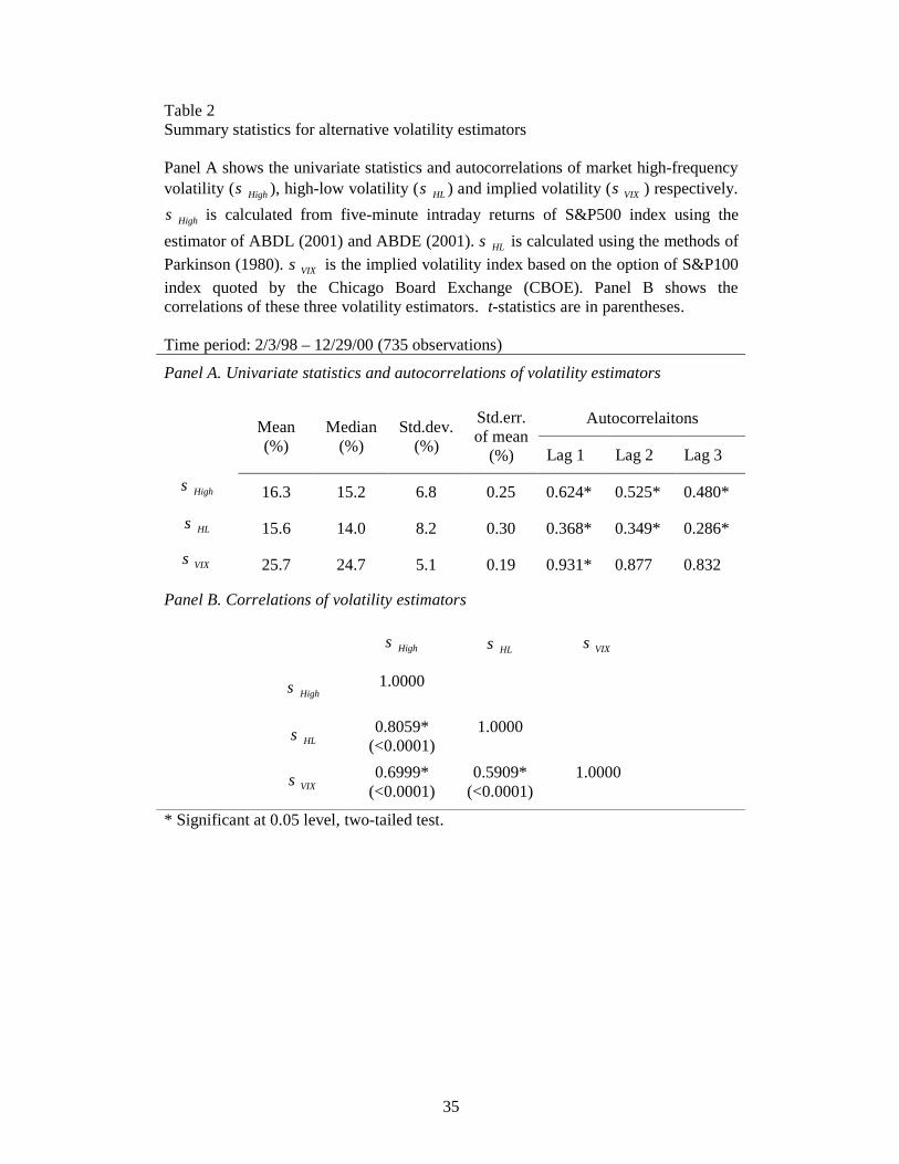
Summary statistics for alternative daily volatility estimators are shown in Table 2.

From Panel A., we can see that all three volatility estimators show substantial positive

autocorrelation. Thus, we should control for this autocorrelation in our later tests.

Moreover, implied volatility ( VIXσ ) is on average higher than volatility estimated

from high-frequency intraday data ( Highσ ) and high-low volatility ( HLσ ). But from the

correlations shown in Panel B., we can see that these three volatility estimators are

highly correlated. The time series of three volatility estimators are shown in Figure 2.

To save space, we will present our results mainly by using high-frequency volatility.

Also, to prevent our inferences from being sensitive to the particular estimators used,

we will repeat all the analyses with the high-low volatility and implied volatility index

time series.

16

4. Empirical Results

4. 1. Daily flow-return relations

Edelen and Warner (2001) document a daily relation between aggregate equity

mutual fund flow and NYSE composite index returns during a time period from

February 1998 to June 1999. Our data on flow come from the same source as theirs

but differs from their data in that we do not have aggregate net flow at equity mutual

funds. Instead, TT provides us with daily data of NAVs, TNAs and flow on a sample

of about 800 funds. Then we aggregate the domestic equity fund flow on our own and

normalize the flow by dividing it by the previous day’s TNA. Thus, we will replicate

their tests of flow-return relation but on a much longer time period to see the

validness of our flow data. The results are shown in Table 3.

Insert Table 3

In Panel A., daily flow is regressed on lagged flow and concurrent and lagged

returns. From Column 1 and Column 2, we can see that flow is highly related to

lagged flow and lagged return. Especially, we use column 2 as expected flow model

used in Panel B. The focus of Panel A. is the concurrent flow-return relation after

controlling for lagged flow and lagged returns, which is presented in Column 3. From

Column 3, the relation between concurrent returns and flow is positive, with a t-

statistics of 2.01. This is consistent with the concurrent flow-return relation presented

in Edelen and Warner (2001).

In Panel B., returns are regressed on concurrent and lagged flow, using both the raw

series and the expected-unexpected flow series. Expected daily flow is taken from the

model in Panel A., Column 2. and unexpected flow is actual minus expected. Column

4 presents the regression of returns on concurrent and lagged raw flow. Column 5 and

Column 6 show the regression of returns on expected and unexpected flow. From

these two columns, we can see that returns are positively related with

contemporaneous unexpected flow but not related with expected flow. The results are

also consistent with Edelen and Warner (2001) though our results using longer time

period are a little weaker than their results.

17

We also perform similar tests during two sub-time periods: during time period

from Feb. 1998 to June 1999 (same time period as Edelen and Warner’s paper), we

get very similar results as Edelen and Warner’s; during time period from July 1999 to

Dec. 2000, the results are a little weaker. Although we do not report the results for the

sub-time periods here to save space, we are confident that our data on flow can reflect

the impact of mutual fund flow on the market.

4. 2. Regression of volatility on aggregate flow

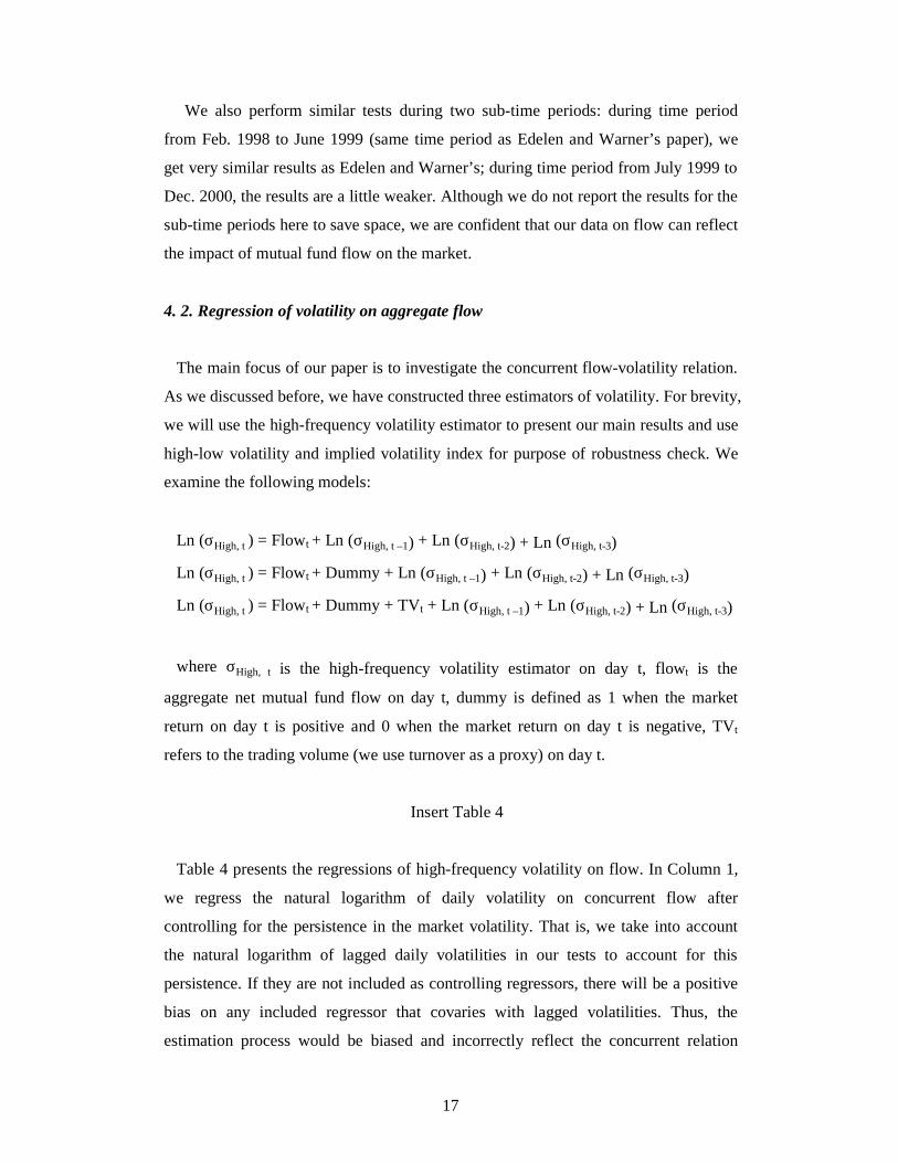
The main focus of our paper is to investigate the concurrent flow-volatility relation.

As we discussed before, we have constructed three estimators of volatility. For brevity,

we will use the high-frequency volatility estimator to present our main results and use

high-low volatility and implied volatility index for purpose of robustness check. We

examine the following models:

Ln (σHigh, t ) = Flowt + Ln (σHigh, t –1) + Ln (σHigh, t-2) + Ln (σHigh, t-3)

Ln (σHigh, t ) = Flowt + Dummy + Ln (σHigh, t –1) + Ln (σHigh, t-2) + Ln (σHigh, t-3)

Ln (σHigh, t ) = Flowt + Dummy + TVt + Ln (σHigh, t –1) + Ln (σHigh, t-2) + Ln (σHigh, t-3)

where σHigh, t is the high-frequency volatility estimator on day t, flowt is the

aggregate net mutual fund flow on day t, dummy is defined as 1 when the market

return on day t is positive and 0 when the market return on day t is negative, TVt

refers to the trading volume (we use turnover as a proxy) on day t.

Insert Table 4

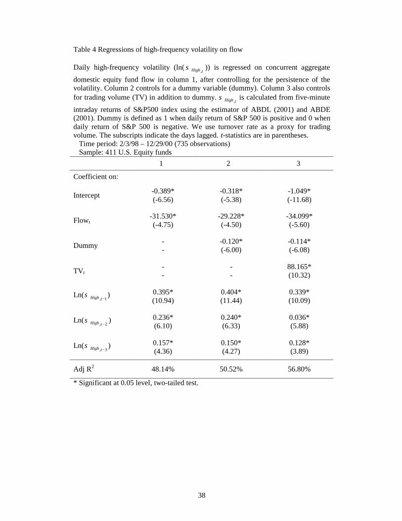
Table 4 presents the regressions of high-frequency volatility on flow. In Column 1,

we regress the natural logarithm of daily volatility on concurrent flow after

controlling for the persistence in the market volatility. That is, we take into account

the natural logarithm of lagged daily volatilities in our tests to account for this

persistence. If they are not included as controlling regressors, there will be a positive

bias on any included regressor that covaries with lagged volatilities. Thus, the

estimation process would be biased and incorrectly reflect the concurrent relation

18

between volatility and flow. From Column 1, the relation between concurrent

volatility and flow is significantly negative, with a t-statistic of –4.75. This implied

that increased aggregate fund flow is associated with decreased market volatility.

In Column 2, we also include a dummy variable as explanatory variable in our

regression given the negative correlation between the S&P 500’s daily returns and

volatility. The dummy variable is defined as 1 when the market return is positive and

0 when the market return is negative. The results indicate that adding the dummy term

does not materially affect the flow coefficient. Moreover, the coefficient of dummy

variable is –0.12 with a t-statistics of –6.0. This implies that bear market is associated

with higher volatility than bull market. This is also consistent with empirical results

(see, e.g., Campbell, Koedijk and Kofman, 2002).

Another issue that catches our attention is the well-documented positive relation

between trading volume and volatility (e.g., karpoff, 1987). As Edelen and Warner

(2001) have suggested, unexpected flow should proxy for subsequent unexpected

institutional trading volume. However, as Edelen (1999) has documented a positive

relation between gross flow (a half of the sum of inflow and outflow) and trading

volume, a positive relation between net flow (inflow minus outflow) and trading

volume does not necessarily follow. Moreover, if mutual fund flow is merely a

substitute for trading volume, then the flow-volatility relation thus gained would be a

spurious consequence of the universal trading-volatility relation. Therefore, we

include trading volume as a regressor in Column 3, to check whether the volatility-

flow coefficient is still statistically significant after controlling for trading volume,

thus getting more consistent and unbiased results. We use turnover rate, that is, daily

trading volume divided by shares outstanding at the end of previous day, as a proxy

for trading volume. The results suggest that flow is still strongly related to market

volatility even after controlling for trading volume.

The evidence so far seems to suggest that there exists a negative relation between

contemporaneous flow and volatility. But a more careful examination will show that

this may be misspecified. We will address this issue in the next sub-section.

4. 3. Regression of volatility on aggregate net inflow and outflow

4.3.1. Misspecification of previous models

19

In the previous part, we find negative concurrent relation between volatility and

flow. In other words, it appears that the larger is the cash flow, the more volatile is the

market. But this may be misspecified because we fail to differentiate between cash

inflow into equity mutual funds and cash outflow from funds. To illustrate this point,

we first look at the classical volume-price change relation.

Insert Figure 3

Karpoff (1987) makes an excellent review on the relation between trading volume

and price changes and presents a model that suggests an asymmetric concurrent

relation between volume and price changes in financial markets. He points out that, as

illustrated in the V shape in Figure 3, there exist a positive relation between volume

and positive price changes and a negative relation between volume and negative price

changes. Moreover, Karpoff argues that tests on linear relation between volume and

price changes per se will yield positive correlations, as shown in the slope of the

dotted line that connects the midpoints of the sides of the V shape in Figure 3. The

positive concurrent relation between volume and price changes is also consistent with

the findings of Morgan (1976), Rogalski (1978), Harris (1984, 1986) and Richardson,

Sefcik, and Thompson (1987). However, Karpoff asserts that tests of the volume-price

change relation without differentiating positive and negative price changes are

misspecified. The reason is not far to see: when it is possible that the relation between

volume and price changes is not monotonic, it is not correct to examine volume-price

change relations across a broad price change range.

We may face a similar scenario when we investigate the volatility-flow relation

given that our previous models are based on the implicit assumption that the

volatility-flow relation is functional and/or monotonic. It is very dangerous because

we will get false results when the volatility and flow relation is not a one-one function.

As far as we know, the tests so far regarding the relation between volatility and flow

(or changes of institutional ownership) do not differentiate positive and negative flow,

or changes of ownership (see, for example, Sias, 1996). Thus, we will revise the

previous models by differentiating positive and negative flow to investigate whether

there exists an asymmetric relation between volatility and flow.

4.3.2. Regressions of volatility on inflow and outflow

20

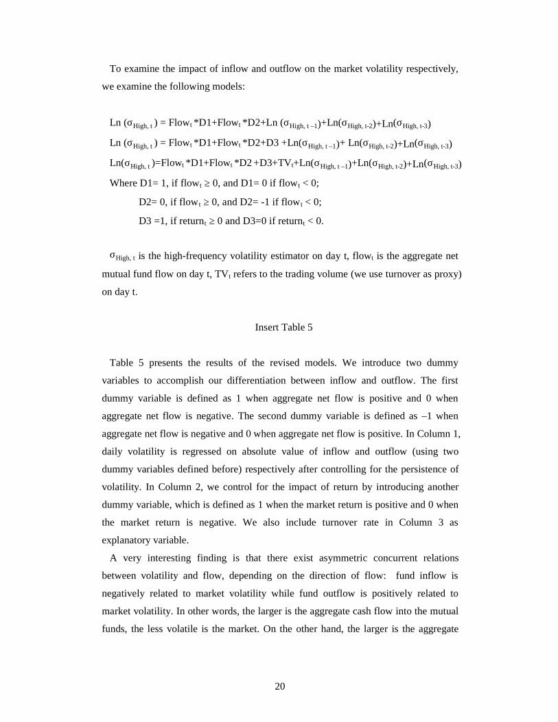
To examine the impact of inflow and outflow on the market volatility respectively,

we examine the following models:

Ln (σHigh, t ) = Flowt *D1+Flowt *D2+Ln (σHigh, t –1)+Ln(σHigh, t-2)+Ln(σHigh, t-3)

Ln (σHigh, t ) = Flowt *D1+Flowt *D2+D3 +Ln(σHigh, t –1)+ Ln(σHigh, t-2)+Ln(σHigh, t-3)

Ln(σHigh, t )=Flowt *D1+Flowt *D2 +D3+TVt+Ln(σHigh, t –1)+Ln(σHigh, t-2)+Ln(σHigh, t-3)

Where D1= 1, if flowt ≥ 0, and D1= 0 if flowt < 0;

D2= 0, if flow t ≥ 0, and D2= -1 if flowt < 0;

D3 =1, if returnt ≥ 0 and D3=0 if returnt < 0. σHigh, t is the high-frequency volatility estimator on day t, flowt is the aggregate net

mutual fund flow on day t, TVt refers to the trading volume (we use turnover as proxy)

on day t.

Insert Table 5

Table 5 presents the results of the revised models. We introduce two dummy

variables to accomplish our differentiation between inflow and outflow. The first

dummy variable is defined as 1 when aggregate net flow is positive and 0 when

aggregate net flow is negative. The second dummy variable is defined as –1 when

aggregate net flow is negative and 0 when aggregate net flow is positive. In Column 1,

daily volatility is regressed on absolute value of inflow and outflow (using two

dummy variables defined before) respectively after controlling for the persistence of

volatility. In Column 2, we control for the impact of return by introducing another

dummy variable, which is defined as 1 when the market return is positive and 0 when

the market return is negative. We also include turnover rate in Column 3 as

explanatory variable.

A very interesting finding is that there exist asymmetric concurrent relations

between volatility and flow, depending on the direction of flow: fund inflow is

negatively related to market volatility while fund outflow is positively related to

market volatility. In other words, the larger is the aggregate cash flow into the mutual

funds, the less volatile is the market. On the other hand, the larger is the aggregate

21

cash flow out of the mutual funds, the more volatile is the market. We illustrate this

asymmetry in Figure 4.

Insert Figure 4

The slopes of solid lines in Figure 4 roughly show the asymmetric relation between

volatility and flow. Moreover, the slope of the dotted line that connects the midpoints

of the two solid lines in the figure above suggests that a negative correlation is likely

to be detected when volatility-flow relation is examined across a broad flow range.

This is just the case— we detect significantly negative concurrent relations between

volatility and flow in the previous sub-section. Thus, previous models that do not take

into account the direction of flow seem to be misspecified.

4. 4. Robustness tests

4. 4. 1. Tests of outliers

Our sample covers about 430 U.S. equity mutual funds, including funds with the

investment objectives varying from aggressive growth to precious metals. In

particular, from Panel A. of Table 1, average flows of funds with the investment

objectives of AG, GI, LG and SF are positive while average flows of funds including

TR, UT, IN and PM are negative. Suppose, if particular funds have especially large

inflow or outflow, the results previously reported in this paper would lose much of

their appeal because it is these outliers rather than the whole sample that drive their

significance.

To test this possibility, we construct a new variable, dispersion rate (DR), as follows:

where Mt refers to the number of funds whose flow on day t is positive, Nt is the

number of funds whose flow on day t is negative, and Tt is the total number of funds

on day t. Table 6 shows the summary statistics of DR. Among 735 observations of

DR, 250 observations are positive with the mean of 0.119 and 485 observations are

negative with the mean of –0.177. Besides, the correlation between flow and DR

variable across the whole time period is 0.63.

t

ttt T

NMDR −=

22

Insert Table 6

We perform similar tests on DR to examine whether any outliers induce this

asymmetric volatility-flow relation. The models are specified as follows:

Ln (σHigh, t ) = DRt *D1+DRt *D2+Ln(σHigh, t –1)+Ln(σHigh, t-2)+Ln (σHigh, t-3)

Ln (σHigh, t ) = DRt *D1+DRt *D2+D3 +Ln (σHigh, t –1)+Ln(σHigh, t-2)+ Ln(σHigh, t-3)

Ln(σHigh, t )=DRt *D1+DRt *D2 +D3+TVt+Ln(σHigh, t –1)+Ln(σHigh, t-2)+Ln(σHigh, t-3)

Where D1= 1, if DRt ≥ 0, and D1= 0 if DRt< 0;

D2= 0, if DRt ≥ 0, and D2= -1 if DRt< 0;

D3 =1, if returnt ≥ 0 and D3=0 if returnt< 0.

σHigh, t is the high-frequency volatility estimator on day t, DRt is the diversion rate as

we defined before on day t, TVt refers to the trading volume (we use turnover as

proxy) on day t. The subscripts indicate the day lagged.

Insert Table 7

The results are shown in table 7. In Column 1, we regress natural logarithm of

volatility on positive DR and absolute value of negative value respectively after

controlling for the persistence of volatility. In Column 2, we also control for the

impact of return by using a dummy variable. In addition, turnover rate is included in

Column 3 as a controlling variable.

The results also show an asymmetric pattern. That is, there is a negative relation

between concurrent volatility and positive dispersion rate and there is a positive

relation between concurrent volatility and absolute value of negative dispersion rate.

The implication of the results is there do not exist outliers in mutual funds that drive

the results.

4. 4. 2. Alternative volatility estimators

As mentioned before, the regressions that use a market volatility estimate as a

dependent variable are subject to an errors-in-the-variables problem. To prevent our

results from being sensitive to particular volatility estimator used, we repeat our tests

23

using two alternative volatility estimators discussed before: high-low volatility and

implied volatility index. For brevity, we only show the results for the most

comprehensive models. The results appear in Table 8.

Insert Table 8

From Table 8, the results using two alternative volatility estimators are very similar

to the results presented before. Nevertheless, the results are a little weaker compared

with those using high-frequency volatility. Thus, we conclude that our results of

asymmetric relation between volatility and flow are not driven due to particular

volatility estimator used.

4. 4. 3. Sub-time periods tests

We also divide our sample period into two sub-time periods: one is from Feb. 1998

to June 1999, which is consistent with the time period in Edelen and Warner (2001);

the other begins at July 1999 and ends with Dec. 2000. Then we replicate all the tests

for the two sub-time periods. Also for brevity, we only show the most comprehensive

models using high-frequency volatility. Table 9 presents the results.

Insert Table 9

The results are on a large part consistent with our previous results. For example, we

get the inflow estimates of –33.4 with the t statistic of –2.94 and –38.1 with the t

statistic of –2.83 for two sub-time periods. At the same time, the outflow estimates

during two sub-time periods are 25.5 with the t statistic of 1.93 and 63.1 with the t

statistic of 2.33 respectively.

4. 4. 4. Other tests

We also perform two additional tests as we mentioned before. First, we would

include global equity (GE) and balanced funds (BL) in our sample to check whether

the results are sensitive to them. Second, we would repeat the analysis, excluding the

December data from our sample to check the dividend effect since most dividends are

distributed in December. However, meaningful changes do not occur in these tests,

but to save space, the results are not reported.

24

5. Discussion: Why Asymmetric Relation?

5.1. Who are decision makers? Two hypotheses.

The asymmetric relation between volatility and flow suggests two, though not

mutually exclusive, stories. On the one hand, individual investors may play an

important part in the market by buying (redeeming) mutual fund shares when market

is up (down). On the other hand, the proactive trading strategies (e.g., herding) of

mutual fund money managers may also drive the market. Then a specific question

arises: who are decision makers? In other words, who are responsible for the

concurrent asymmetric volatility-flow relation, individual investors or mutual fund

managers?

It is well known that mutual funds are required by law to redeem shares on a daily

basis, thus making mutual fund shares a very liquid investment. This liquidity service,

as pointed out in Edelen (1999), forces mutual fund to engage in a substantial amount

of uninformed, liquidity-motivated trading, and this liquidity-motivated trading makes

up a material fraction of the fund’s overall trading activity. Then the question is

whether this kind of liquidity-motivated trading is sufficient to deliver a meaningful

movement in stock market volatility. Harris and Raviv (1993) and Shalen (1993)

propose the dispersion of beliefs models, which show that a greater dispersion of

beliefs, that is, a wider dispersion of expectations in the current and preceding rounds

of trade, will create excess price variability relative to the equilibrium value.

Especially, as Shalen (1993) has pointed out, uninformed (or less-informed) investors

have difficulty in interpreting the noisy signals of price change, that is, they cannot

differentiate the short-term random liquidity demand from the overall fundamental

changes in supply and demand. This could result in a general discrepancy about the

true price embodied in the revealed information. Thus this kind of wider dispersion of

beliefs would make uninformed investors react to all changes in prices as if they truly

reflect the information. Moreover, uninformed investors tend to revise their beliefs

more frequently, thus resulting in slower disappearance of price fluctuations from

their trading than those from their informed counterparts after the new public

information. In these ways, uninformed investors would more likely overreact to

fundamental price movements, which would lead to increased price volatility.

25

Therefore, as mutual fund investors are uninformed or relatively uninformed (Warther,

1995), they possess no information or receive information on a delayed or second-

hand basis, if they receive information at all, to the extent that mutual funds facilitate

their entry into the market, and to the extend flow should proxy for the liquidity-

motivated trading, mutual fund flow would inevitably induce greater price volatility.

However, this seems to tell only part of the stories. As we discussed before, the

herding and positive-feedback trading strategies of mutual fund managers would exert

significant influence on the market. Nevertheless, herding and positive-feedback

trading does not necessarily destabilize or stabilize the market. For example, herding

would destabilize the market when mutual fund managers ignore their own

information about fundamentals and mimic the trading of others. Yet, herding might

stabilize the market by speeding up the adjustment of prices to new fundamentals and

making the market more efficient when funds react to the same fundamental

information in a timely manner. We will show later that our findings will unite these

two stories in a consistent framework.

5.2. Information effect

Chan and Lakonishok (1993) discuss the differences in the information content of

institutional trades. They argue that “Since an institutional investor typically does not

hold the market portfolio, the choice of a particular issue to sell, out of the limited

alternatives in a portfolio, does not necessarily convey negative information. Rather,

the stocks that are sold may already have met the portfolio’s objectives, or there may

be other mechanical rules, unrelated to expectations about future performance, for

reducing a position. As a result, there are many liquidity-motivated reasons to dispose

of a stock. In contrast, the choice of one specific issue to buy, out of the numerous

possibilities on the market, is likely to convey favorable firm-specific news.” Implied

in this argument is the suggestion that buy orders of institutions convey more

information than sell orders. In addition, Keim and Madhavan (1995) provide another

channel through which the information content of buys is greater than sales:

institutional traders can choose among various potential assets; however, their sales

are limited to the assets they already own due to the short sales restriction. Keim and

Madhavan (1997) also show that trading costs for buy-initiated trades exceed seller-

initiated trades and their findings are consistent with the differences of information

26

content of buys and sales. Saar (2001) develops a model which shows that the trading

strategy of mutual fund managers creates a difference between the information

content of buys and sells. He proposes a “prototypical” mutual fund which describes

the behavior and constraints of mutual funds. Specifically, he points out that the

asymmetry is mainly driven by two factors: the first is the ability of portfolio

managers to gather, analyze and optimally use the private information; the second is a

set of trading constraints (e.g., restriction on the use of leverage and short sales) that

portfolio managers face.

5.3. Explanation: asymmetric relation

Our findings of asymmetric concurrent volatility-flow relation are consistent with

the differences of information content of mutual funds’ buying and selling behavior

discussed above. When the market is up, individual investors tend to buy mutual fund

shares. Thus, large sums of cash flow into mutual funds and mutual fund managers

will invest the money in a diversified portfolio. As pointed out by Saar (2001), mutual

funds will devote substantial resources to gathering and analyzing private information

and make investment decisions based on predictions and recommendations of their

research departments. Under such circumstances, mutual funds might appear to herd

if they all react to the same fundamental information. Thus, their trading or herding

behaviors tend to stabilize the market by speeding up the adjustment of the prices to

new fundamentals. If this is the case, we would expect negative relation between

market volatility and aggregate mutual fund flow. That is just what we have found:

more fund inflow is associated with less volatile market.

By contrast, during down market periods, individual investors tend to redeem

mutual fund shares and large sums of money exit the mutual funds. Besides, mutual

funds are subject to a set of constraints (Saar, 2001). For example, use of leverage is

restricted in mutual fund charters; short sales are also forbidden. Hence, fund

managers are forced to sell stocks from their portfolios to satisfy the liquidity

requirement of individual investors more often than are forced to buy stocks.

Moreover, fund managers may tend to over-react to market information or sell stocks

in a panic when market is down. Thus, fund managers are less rational and their

trading or herding on selling stocks contains less information than their trading or

herding on buying stocks. As we discussed before, such herding will drive the prices

27

away from the assets’ fundamental values and destabilize the market. This is also

consistent with our findings: the more is the aggregate mutual fund outflow, the more

volatile is the market.

Taken together, we link the impact of individual investors and mutual fund

managers in a unified framework and provide a potential explanation for our findings.

A potential testing of our results is to investigate the impact of herding on buys or

sales on the market respectively. However, this is beyond the availability of our data

and thus the scope of this paper. Future tests on this issue will help shed more light on

our asymmetric results.

6. Conclusion

In this paper, we use daily data to directly investigate the concurrent volatility-flow

relation. Our high frequency data enable us to conduct rigorous tests which offer new

evidence. Our studies are expected to shed light on the impact of institutional trading

on the market and be of importance to investors, practitioners, academicians and

regulators.

Our initial evidence suggests a significantly negative contemporaneous relation

between volatility and aggregate net mutual fund flow across the whole flow range.

However, additional insight on this issue is gained by differentiating the data between

inflow and outflow. An important finding emerges after we take into account the

direction of aggregate net flow: there is a marked asymmetry between the impact of

inflow and outflow on the market. Increases in aggregate net inflow are accompanied

by less volatile market; however, increases in aggregate net outflow are associated

with more volatile market.

We discuss the potential explanations for our findings of asymmetric concurrent

volatility-flow relation and suggest the joint roles played by individual investors and

mutual fund managers in the market. Our results are also consistent with the

differences of information content of mutual funds’ buys and sales.

28

Reference:

Andersen, T.G., Bollerslev, T., Diebold, F.X. and Ebens, H., 2001. “The distribution

of realized stock return volatility.” Journal of Financial Economics 61, 43-76

Andersen, T.G., Bollerslev, T., Diebold, F.X. and Labys, P., 2001. “The distribution

of realized exchange rate volatility.” Journal of the American Statistical Association

96, 42-55

Arbel, A., Carvell, S. and Strebel, P., 1983. “Giraffes, institutions and neglected

firms.” Financial Analysts Journal 39, 55-63

Badrinath, S.G., Gay, G.D. and Kale, 1989. “Patterns of institutional investment,

prudence, and the managerial safety-net hypothesis.” Journal of risk and insurance 55,

605-629

Bikhchandani, S., Hirshleifer, D. and Welch, I., 1992. “A theory of fads, fashion,

custom, and cultural change as informational cascades.” Journal of Political Economy

100, 992-1026

Brennan, M.J., 1995. "The individual investor." Journal of Financial Research 18, 59-

74

Busse, J.A., 1999. “Volatility timing in mutual funds: evidence from daily returns.”

The Review of Financial Studies 12, 1009-1041

Campbell, J.Y., 1987. “Stock returns and the term structure.” Journal of Financial

Economics 18, 373-399

Campbell, R., Koedijk, K. and Kofman, P., 2002. "Increased correlation in bear

markets." Financial Analysts Journal 58, 87-94

29

Chalmers, J.M.R., Edelen, R.M. and Kadlec G.B., 2000. “The wildcard option in

transacting mutual-fund shares.” Working paper, University of Pennsylvania

Chan, L. and Lakonishok, J., 1993. “Institutional trades and intraday stock price

behavior.” Journal of Financial Economics 33, 173-200

Chan, L. and Lakonishok, J., 1995. “The behavior of stock prices around institutional

trades.” Journal of Finance 50, 1147-1174

Chan, L. and Lakonishok, J., 1997. “Institutional equity trading costs: NYSE versus

NASDAQ.” Journal of Finance 52, 713-735

Chan, L., Jegadeesh, N. and Lakonishok, J., 1996. “Momentum strategies.” Journal of

Finance 51, 1681-1713

Chopra, N., Lakonishok, J. and Ritter, J., 1992. "Measuring abnormal performance--

Do stocks overreact?" Journal of Financial Economics 49, 235-268

DeLong, J.B., Shleifer, A., Summers, L.H. and Waldmann, R.J., 1990a. “Noise trader

risk in financial markets.” Journal of Political Economy 98, 703-739

DeLong, J.B., Shleifer, A., Summers, L.H. and Waldmann, R.J., 1990b. “Positive

feedback investment strategies and destabilizing rational speculation.” Journal of

Finance 45, 379-395

DeLong, J.B., Shleifer, A., Summers, L.H. and Waldmann, R.J., 1991. “The survival

of noise traders in financial markets.” Journal of Business 64, 1-19

Dreman, D., 1979. “Contrarian investment strategy: the psychology of stock market

success.” (Random House, New York).

Edelen, R.M., 1999. "Investor flows and the assessed performance of open-end

mutual funds." Journal of Financial Economics 53, 439-466

30

Edelen, R.M. and Warner, J.B., 2001. “Aggregate price effects of institutional trading:

a study of mutual fund flow and market returns.” Journal of Financial Economics 59,

195-220

French, K.R., Schwert, G.W. and Stambaugh, 1987. “Expected stock returns and

volatility.” Journal of Financial Economics 19, 3-30

Glosten, L.R., Jagannathan, R. and Runkle, D.E., 1993. “On the relation between the

expected value and the volatility of the nominal excess return on stocks.” Journal of

Finance 48, 1779-1801

Goetzmann, W.N., Ivkovic, Z. and Rouwenhorst, K.G., 2000. “Day trading

international mutual funds: evidence and policy solutions.” Working paper, Yale

University.

Gompers, P. and Metrick, A., 2001. "Institutional investors and equity prices." The

Quarterly Journal of Economics 116, 229-259

Greene, J.T., 2000. “The dilution impact of daily fund flows on open-end mutual

funds.” Working paper, Georgia State University.

Harris, L., 1984. "Transactions data tests of the mixture of distributions hypothesis."

Working paper, Univ. of Southern CA.

Harris, L., 1986. "Cross-security tests of the mixture of distributions hypothesis."

Journal of Financial and Quantitative Analysis 21, 39-46

Harris, M. and Artur, R., 1993. "Differences of opinion make a horse race." Review

of Financial Studies 6, 473-506

Haugen, R.A., Talmor, E. and Torous, W.N., 1991. “The effect of volatility changes

on the level of stock prices and subsequent expected returns.” Journal of finance 46,

985-1007

31

Hirshleifer, D., Subrahmanyam, A. and Titman, S., 1994. “Security analysis and

trading patterns when some investors receive information before others.” Journal of

Finance 49, 1665-1698

Jegadeesh, N. and Titman, S., 1993. “Returns to buying winners and selling losers:

implications for stock market efficiency.” Journal of Finance 48, 65-91

Jones, C. and Lipson, M., 1999. “Execution costs of institutional equity orders.”

Journal of Financial Intermediation 8, 123-140

Karpoff, J.M., 1987. "The relation between price changes and trading volume: a

survey." Journal of Financial and Quantitative Analysis 22, 109-126

Keim, D. and Madhavan, A., 1995. "Anatomy of the trading process: empirical

evidence on the behavior of institutional trades" Journal of Financial Economics 37,

371-398

Keim, D. and Madhavan, A., 1997. “Transactions costs and investment style: an inter-

exchange analysis of institutional equity trades.” Journal of Financial Economics 46,

103-131

Kothare, M. and Laux, P.A., 1995. "Trading costs and the trading systems for Nasdaq

stocks." Financial Analysts Journal 51, 42-53

Lakonishok, J., Shleifer, A. and Vishny, R.W., 1992. “The impact of institutional

trading on stock prices.” Journal of Financial Economics 32, 23-44

Lakonishok, J., Shleifer, A. and Vishny, R.W., 1994. "Contrarian investment,

extrapolation, and risk." Journal of Finance 49, 1541-1578

Lockwood, L.J. and Linn, S.C., 1990. “An examination of stock market return

volatility during overnight and intraday periods, 1964-1989.” Journal of Finance 45,

591-601

32

Xu Yexiao. and Malkiel B.G, 2002. “Investigating the behavior of idiosyncratic

volatility.” Forthcoming in Journal of Business

Morgan, I.G., 1976. "Stock prices and heteroskedasticity." Journal of Business 49,

496-508

Nofsinger, J.R. and Sias, R.W., 1999. “Herding and feedback trading by institutional

and individual investors.” Journal of Finance 54, 2263-2295

Parkinson, M., 1980. “The extreme value method for estimating the variance of the

rate return.” Journal of Business 53, 61-66

Reilly, F.K., 1979. “How institutional trading reduces market volatility.” Journal of

Portfolio Management 5, 11-17

Richardson, G., Sefcik, S.E. and Thompson, R., 1986. "A test of dividend irrelevance

using volume reaction to a change in dividend policy." Journal of Financial

Economics 17, 313-333

Rogalski, R.J., 1978. "The dependence of prices and volume." The Review of

Economics and Statistics 36, 268-274

Saar, G., 2001. "Price impact asymmetry of block trades: an institutional trading

explanation." Review of Financial Studies 14, 1153-1181

Scharfstein, D.S. and Stein, J.C., 1990. "Herd behavior and investment." American

Economic Review 80, 465-479

Schwert, G.W., 1989. “Why does stock market volatility change over time?” Journal

of Finance 44, 1115-1153

Shalen, C.T., 1993. "Volume, volatility, and the dispersion of beliefs." Review of

Financial Studies 6, 405-434

33

Sias, R.W. and Starks, L.T., 1997. "Return autocorrelation and institutional

investors." Journal of Financial Economics 46, 103-131

Sias, R.W., 1996. “Volatility and the institutional investor.” Financial analysts journal

52, 13-20

Warther, V., 1998. “Has the rise of mutual funds increased market instability?”

Brookings-Wharton Papers on Financial Services, 239-262

Warther, V., 1995. “Aggregate mutual fund flows and security returns.” Journal of

Financial Economics 39, 209-235

Wermers, R., 1999. "Mutual fund herding and the impact on stock prices." Journal of

Finance 54, 581-622

Whitelaw, R.F., 1994. “Time variations and covariations in the expectation and

volatility of stock market returns.” Journal of Finance 49, 515-541

Zweig, M., 1973. "An investor expectations stock price predictive model using

closed-end fund premiums." Journal of Finance 28, 67-78

34

Table 1 Summary statistics for daily mutual fund flow Our data on daily flow (new subscriptions less redemptions), NAV and total net assets (TNA) come from Trim Tabs (TT) financial services of Santa Rosa, California. We match the whole sample of about 850 mutual funds in TT with those in CRSP survivor-bias free US mutual fund database and classify the mutual funds by the investment objectives defined by Investment Company Institute (ICI). Included in our sample of all U.S. equity funds are funds from aggressive growth (AG) to precious metals (PM). We apply two filters detailed in the main text, the absolute-value filter and the Reversal filters, to the TNA and NAV series and aggregate the two series. Flow is defined as the one-day percentage change in aggregate TNA, less the one-day percentage change in the aggregate NAV. Distributions are not accounted for in these data.

Time period: 2/3/98 – 12/29/00 (735 observations) Sample: 411 U.S. Equity funds

Panel A. Univariate statistics and autocorrelations of fund flow

Autocorrelations Fund investment objective

Mean (b.p.)

Median (b.p.)

Std. dev. (b.p.)

Std.err of

mean (b.p.)

Lag1 Lag2 Lag5

Aggressive growth (AG) 4.54 3.54 25.6 0.95 -0.023* -0.144* 0.094

Growth and income (GI) 1.33 1.11 8.9 0.33 -0.193* 0.051 0.129*

Long-term growth (LG) 3.63 2.57 23.3 0.86 -0.065* -0.310* 0.003

Sector funds (SF) 3.44 1.33 40.0 1.48 -0.223* -0.075* -0.012

Total return (TR) -4.44 -4.35 18.2 0.67 -0.076* 0.031 0.122*

Utility funds (UT) -1.91 -2.97 38.0 1.41 -0.361* 0.009* 0.041

Income (IN) -1.68 -2.18 13.0 0.48 -0.076* 0.071 0.140*

Precious metals (PM) -4.77 -21.3 198.0 7.33 -0.147* -0.237* -0.034

All U.S. equity funds 2.94 1.63 15.6 0.58 -0.091* -0.227* 0.060

Panel B. Univariate statistics of aggregate net inflow and outflow

Obs. Mean (b.p.)

Median (b.p.)

Std. dev. (b.p.)

Std. err of mean (b.p.)

Aggregate net inflow 416 11.83 9.00 12.8 0.63

Aggregate net outflow 319 -8.62 -6.69 10.5 0.59

* Significant at 0.05 level, two-tailed test.

35

Table 2 Summary statistics for alternative volatility estimators Panel A shows the univariate statistics and autocorrelations of market high-frequency volatility ( Highσ ), high-low volatility ( HLσ ) and implied volatility ( VIXσ ) respectively.

Highσ is calculated from five-minute intraday returns of S&P500 index using the estimator of ABDL (2001) and ABDE (2001). HLσ is calculated using the methods of Parkinson (1980). VIXσ is the implied volatility index based on the option of S&P100 index quoted by the Chicago Board Exchange (CBOE). Panel B shows the correlations of these three volatility estimators. t-statistics are in parentheses. Time period: 2/3/98 – 12/29/00 (735 observations)

Panel A. Univariate statistics and autocorrelations of volatility estimators

Autocorrelaitons Mean

(%) Median

(%) Std.dev.

(%)

Std.err. of mean

(%) Lag 1 Lag 2 Lag 3

Highσ 16.3 15.2 6.8 0.25 0.624* 0.525* 0.480*

HLσ 15.6 14.0 8.2 0.30 0.368* 0.349* 0.286*

VIXσ 25.7 24.7 5.1 0.19 0.931* 0.877 0.832

Panel B. Correlations of volatility estimators

Highσ HLσ VIXσ

Highσ 1.0000

HLσ 0.8059*

(<0.0001) 1.0000

VIXσ 0.6999*

(<0.0001) 0.5909*

(<0.0001) 1.0000

* Significant at 0.05 level, two-tailed test.

36

Table 3 Contemporaneous relations between Returns and flow In Panel A., daily flow is regressed on current and past observations of market returns of NYSE index (Rt) and past observations of flow. In Panel B., daily returns of NYSE index are regressed on concurrent and lagged daily flow (Flow t) in column 4, and on concurrent and lagged unexpected daily flow (Uflowt) and concurrent expected daily flow (Eflowt) in column 5 and 6. Expected daily flow is taken from Panel A, column 2. Unexpected flow is actual minus expected. The subscripts indicate the days lagged. t-statistics are in parentheses.

Time Period: 2/3/98-12/29/00(735 observations) Sample: 411 U.S. Equity funds

Panel A. Flow dependence on returns and past flow

1 2 3 Coefficient on:

Intercept 0.00031* (6.2)

0.00031* (8.2)

0.00030* (8.1)

Rt - -

- -

0.009* (2.01)

Rt-1 0.068* (15.1)

0.069* (15.6)

0.066* (15.1)

Rt-2 -0.036* (-5.9)

-0.035* (-8.0)

-0.038* (-8.5)

Rt-3 -0.010 (-1.87)

-0.009 (-1.67)

- -

Flowt-1 - -

-0.077* (-2.11)

-0.077* (-2.12)

Flowt-2 - -

-0.220* (-6.03)

-0.225* (-6.18)

R2 28.5% 32.3% 33.3%

Panel B. Returns dependence on flow

Raw flow 4 Exp.-unexp. flow 5 6 Coefficient on: Coefficient on:

Intercept 0.00012 (0.25) Intercept 0.00043

(0.01) 0.00013 (1.07)

Flowt 0. 317* (1.97) Uflowt

0. 663* (2.48)

0.629* (2.01)

Flowt-1 0.021 (0.08) Uflowt-1

0.006 (0.02)

- -

Flowt-2 -0.038 (-0.14) Uflowt-2

0.273 (0.81)

- -

Flowt-3 -0.00002 (-0.00) Uflowt-3

-0.325 (-1.03)

- -

Flowt-4 -0.119 (-0.44) Uflowt-4

-0.089 (-0.28)

- -

37

Flowt-5 0.115 (0.43) Uflowt-5

0.166 (0.52)

- -

Eflowt 0.483 (0.98)

0.459

(1.01)

R2 1.0% 2.3% 1.9%

* Significant at 0.05 level, two-tailed test.

38

Table 4 Regressions of high-frequency volatility on flow Daily high-frequency volatility (ln(

tHigh ,σ )) is regressed on concurrent aggregate

domestic equity fund flow in column 1, after controlling for the persistence of the volatility. Column 2 controls for a dummy variable (dummy). Column 3 also controls for trading volume (TV) in addition to dummy.

tHigh ,σ is calculated from five-minute

intraday returns of S&P500 index using the estimator of ABDL (2001) and ABDE (2001). Dummy is defined as 1 when daily return of S&P 500 is positive and 0 when daily return of S&P 500 is negative. We use turnover rate as a proxy for trading volume. The subscripts indicate the days lagged. t-statistics are in parentheses.

Time period: 2/3/98 – 12/29/00 (735 observations) Sample: 411 U.S. Equity funds

1 2 3

Coefficient on:

Intercept -0.389* (-6.56)

-0.318* (-5.38)

-1.049* (-11.68)

Flowt -31.530* (-4.75)

-29.228* (-4.50)

-34.099* (-5.60)

Dummy - -

-0.120* (-6.00)

-0.114* (-6.08)

TVt - -

- -

88.165* (10.32)

Ln(1, −tHighσ ) 0.395*

(10.94) 0.404* (11.44)

0.339* (10.09)

Ln(2, −tHighσ ) 0.236*

(6.10) 0.240* (6.33)

0.036* (5.88)

Ln(3, −tHighσ ) 0.157*

(4.36) 0.150* (4.27)

0.128* (3.89)

Adj R2 48.14% 50.52% 56.80%

* Significant at 0.05 level, two-tailed test.

39

Table 5 Regressions of high-frequency volatility on aggregate net inflow and outflow Daily high-frequency volatility (ln(

tHigh ,σ )) is regressed on concurrent aggregate net

inflow and outflow (using two dummy variables, dummy1 and dummy 2) in column 1, after controlling for the persistence of the volatility. Column 2 controls for a dummy variable (dummy 3). Column 3 also controls for trading volume (TV) in addition to dummy 3.

tHigh ,σ is calculated from five-minute intraday returns of S&P500 index

using the estimator of ABDL (2001) and ABDE (2001). Dummy 1 is defined as 1 when aggregate flow is positive and 0 when aggregate flow is negative. Dummy 2 is defined as –1 when aggregate flow is negative and 0 when aggregate flow is positive. Dummy 3 is defined as 1 when daily return of S&P 500 is positive and 0 when daily return of S&P 500 is negative. We use turnover rate as a proxy for trading volume. The subscripts indicate the days lagged. t-statistics are in parentheses.

Time period: 2/3/98 – 12/29/00 (735 observations) Sample: 411 U.S. Equity funds

1 2 3

Coefficient on:

Intercept -0.389* (-6.45)

-0.315* (-5.23)

-1.296* (-13.83)

Flowt*dummy1 -31.647* (-3.32)

-31.215* (-3.35)

-36.819* (-4.37)

Flowt*dummy2 31.335* (2.39)

25.934* (2.02)

28.035* (2.42)

Dummy3 - -

-0.121* (-6.01)

-0.115* (-6.32)

TVt - -

- -

110.740* (12.85)

Ln(1, −tHighσ ) 0.395*

(10.93) 0.404* (11.43)

0.317* (9.70)

Ln(2, −tHighσ ) 0.236*

(6.09) 0.240* (6.33)

0.200* (5.82)

Ln(3, −tHighσ ) 0.157*

(4.36) 0.150* (4.27)

0.127* (3.99)

Adj R2 48.07% 50.46% 59.61%

* Significant at 0.05 level, two-tailed test.

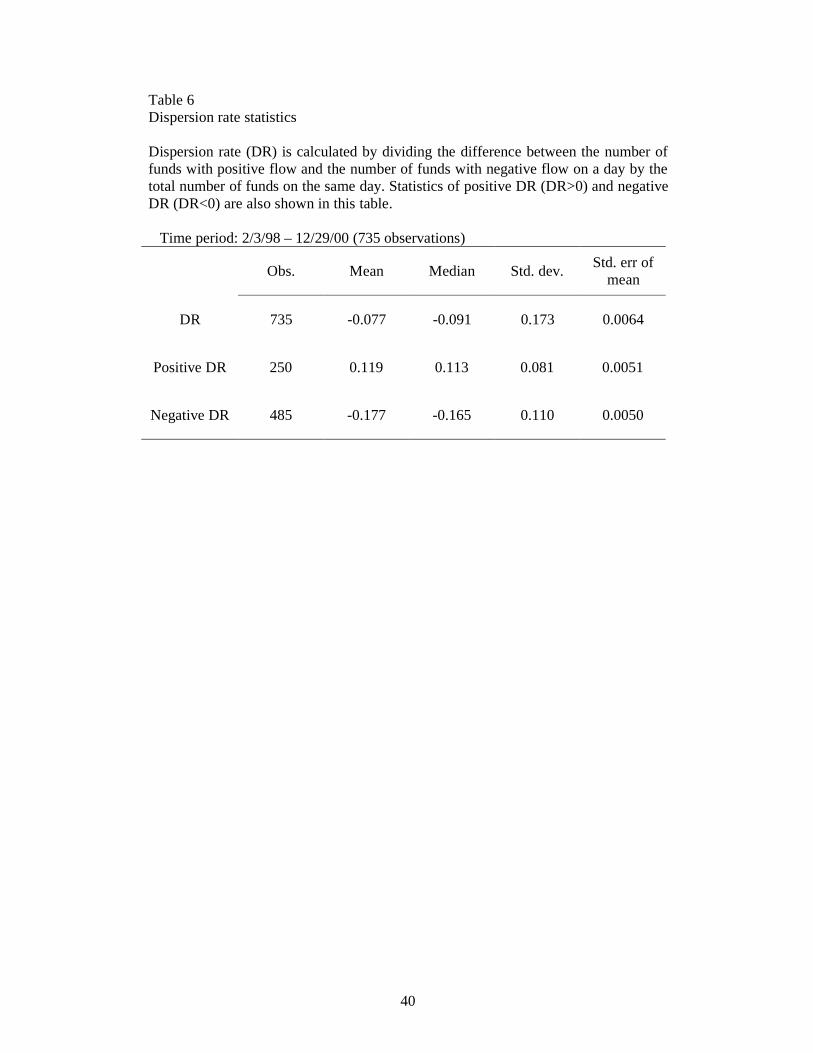
40

Table 6 Dispersion rate statistics Dispersion rate (DR) is calculated by dividing the difference between the number of funds with positive flow and the number of funds with negative flow on a day by the total number of funds on the same day. Statistics of positive DR (DR>0) and negative DR (DR<0) are also shown in this table.

Time period: 2/3/98 – 12/29/00 (735 observations)

Obs. Mean Median Std. dev. Std. err of mean

DR 735 -0.077 -0.091 0.173 0.0064

Positive DR 250 0.119 0.113 0.081 0.0051

Negative DR 485 -0.177 -0.165 0.110 0.0050

41

Table 7 Regression of high-frequency volatility on dispersion rate Daily high-frequency volatility (ln(

tHigh ,σ )) is regressed on positive and negative

dispersion rate (DR) (using two dummy variables, dummy1 and dummy 2) in column 1, after controlling for the persistence of the volatility. Column 2 controls for a dummy variable (dummy 3). Column 3 also controls for trading volume (TV) in addition to dummy 3.

tHigh ,σ is calculated from five-minute intraday returns of

S&P500 index using the estimator of ABDL (2001) and ABDE (2001). DR is calculated by dividing the difference between the number of funds with positive flow and the number of funds with negative flow on a day by the total number of funds on the same day. Dummy 1 is defined as 1 when aggregate flow is positive and 0 when aggregate flow is negative. Dummy 2 is defined as –1 when aggregate flow is negative and 0 when aggregate flow is positive. Dummy 3 is defined as 1 when daily return of S&P 500 is positive and 0 when daily return of S&P 500 is negative. We use turnover rate as a proxy for trading volume. The subscripts indicate the days lagged. t-statistics are in parentheses.

Time period: 2/3/98 – 12/29/00 (735 observations) 1 2 3

Coefficient on:

Intercept -0.517* (-8.24)

-0.443* (-7.13)

-1.306* (-13.72)

DRt*dummy1 -0.380* (-2.36)

-0.362* (-2.31)

-0.235# (-1.63)

DRt*dummy2 0.493* (4.99)

0.500* (5.20)

0.496* (5.44)

Dummy3 - -

-0.125* (-6.40)

-0.121* (-6.72)

TVt - -

- -

98.612* (11.35)

Ln(1, −tHighσ ) 0.357*

(9.90) 0.365* (10.39)

0.298* (9.04)

Ln(2, −tHighσ ) 0.233*

(6.20) 0.238* (6.51)

0.195* (5.73)

Ln(3, −tHighσ ) 0.159*

(4.52) 0.152* (4.43)

0.134* (4.24)

Adj R2 50.42% 53.01% 60.08%

* Significant at 0.05 level, two-tailed test # Significant at 0.10 level, two-tailed test

42

Table 8 Dependence of high-low volatility and implied volatility on aggregate net inflow and outflow Controlling for the persistence of the volatility, trading volume (TV) and a dummy variable (dummy 3), daily high-low volatility (Ln( tHL ,σ )) and implied volatility (Ln( tVIX ,σ )) are regressed on concurrent aggregate net inflow and outflow (using two dummy variables, dummy1 and dummy 2) in column 1 and column 2 respectively.

tVIX ,σ is calculated using the methods of Parkinson (1980). tVIX ,σ is the implied volatility index based on the option of S&P100 index quoted by the Chicago Board Exchange (CBOE). Dummy 1 is defined as 1 when aggregate flow is positive and 0 when aggregate flow is negative. Dummy 2 is defined as –1 when aggregate flow is negative and 0 when aggregate flow is positive. Dummy 3 is defined as 1 when daily return of S&P 500 is positive and 0 when daily return of S&P 500 is negative. We use turnover rate as a proxy for trading volume. The subscripts indicate the days lagged.

Time period: 2/3/98 – 12/29/00 (735 observations) Sample: 411 U.S. Equity funds

1 2

Ln( tHL ,σ ) Ln( tVIX ,σ )

Estimate T-value Estimate T-value

Intercept -1.535* -11.97 -0.034# -1.67

Flowt*dummy1 -39.671* -3.03 -4.835* -2.69

Flowt*dummy2 48.481* 2.71 4.066# 1.82

Dummy3 -0.160* -5.68 -0.085* -22.96

TVt 114.305* 9.20 3.885* 2.34

Ln( 1−tσ ) 0.151* 4.43 0.950* 90.32

Ln( 2−tσ ) 0.237* 7.00 - -

Ln( 3−tσ ) 0.133* 3.94 - -

Adj R2 34.70% 94.02%

* Significant at 0.05 level, two-tailed test. # Significant at 0.10 level, two-tailed test.

43

Table 9 Sub-period check of high-frequency volatility on aggregate net inflow and outflow Controlling for the persistence of the volatility, trading volume (TV) and a dummy variable (dummy 3), daily high-frequency volatility (ln(

tHigh ,σ )) is regressed on

concurrent aggregate net inflow and outflow (using two dummy variables, dummy1 and dummy 2)during two sub-time periods in column 1 and column 2.

tHigh ,σ is

calculated from five-minute intraday returns of S&P500 index using the estimator of ABDL (2001) and ABDE (2001). Dummy 1 is defined as 1 when aggregate flow is positive and 0 when aggregate flow is negative. Dummy 2 is defined as –1 when aggregate flow is negative and 0 when aggregate flow is positive. Dummy 3 is defined as 1 when daily return of S&P 500 is positive and 0 when daily return of S&P 500 is negative. We use turnover rate as a proxy for trading volume. The subscripts indicate the days lagged. t-statistics are in parentheses.

Time period 1: 2/3/98 – 6/30/99 (355 observations) Time period 2: 7/1/99 – 12/29/00 (380 observations) Sample: 411 U.S. Equity funds

1 2

Time period 1 Time period 2

Estimate T-value Estimate T-value

Intercept -1.064* -7.80 -1.442* -10.56

Flowt*dummy1 -33.404* -2.94 -38.113* -2.83

Flowt*dummy2 25.459# 1.93 63.096* 2.33

Dummy3 -0.137* -5.13 -0.095* -3.69

TVt 132.201* 7.12 107.138* 9.48

Ln(1, −tHighσ ) 0.357* 7.42 0.300* 6.53

Ln(2, −tHighσ ) 0.236* 4.54 0.166* 3.51

Ln(3, −tHighσ ) 0.166* 3.47 0.086* 1.96

Adj R2 59.61% 52.69%

* Significant at 0.05 level, two-tailed test. # Significant at 0.10 level, two-tailed test.

44

Fig. 1. Time series of daily aggregate U.S. equity mutual fund flow. The figure shows the time series of daily aggregate domestic equity mutual fund flow. Our data on flow (new subscriptions less redemptions) come from Trim Tabs (TT) financial services of Santa Rosa, California. Flow is defined as the one-day percentage change in aggregate TNA, less the one-day percentage change in the aggregate NAV. The sample covers the period from February 3, 1998 through December 29, 2000, for a total of 735 observations.

980203 980822 990310 990926 000413 001030-0.020

-0.015

-0.010

-0.005

0.000

0.005

0.010

0.015

0.020

FLO

W

45

Fig. 2. Time series of different volatility estimators. The figure shows time series of three different market volatility estimators: high-frequency volatility ( Highσ ) in (a), high-low volatility ( HLσ ) in (b) and implied volatility ( VIXσ ) in (c). Highσ is calculated from five-minute intraday returns of S&P500 index using the estimator of ABDL (2001) and ABDE (2001). HLσ is calculated using the methods of Parkinson (1980). VIXσ is the implied volatility index based on the option of S&P100 index quoted by the Chicago Board Exchange (CBOE). The sample covers the period from February 3, 1998 through December 29, 2000, for a total of 735 observations.

980203 980630 981124 990420 990914 000208 000704 001128 0.0

0.1

0.2

0.3

0.4

0.5

0.6

Vola

tility

σHigh

Figure 2 (a) High-freq. volatility

980203 980630 981124 990420 990914 000208 000704 001128 0.0

0.1

0.2

0.3

0.4

0.5

0.6

Vola

tility

σHL

Figure 2 (b) High-low volatility

980203 980630 981124 990420 990914 000208 000704 001128

0.15

0.20

0.25

0.30

0.35

0.40

0.45

0.50

Vola

tility

Figure 2 (c) Implied volatility

σVIX

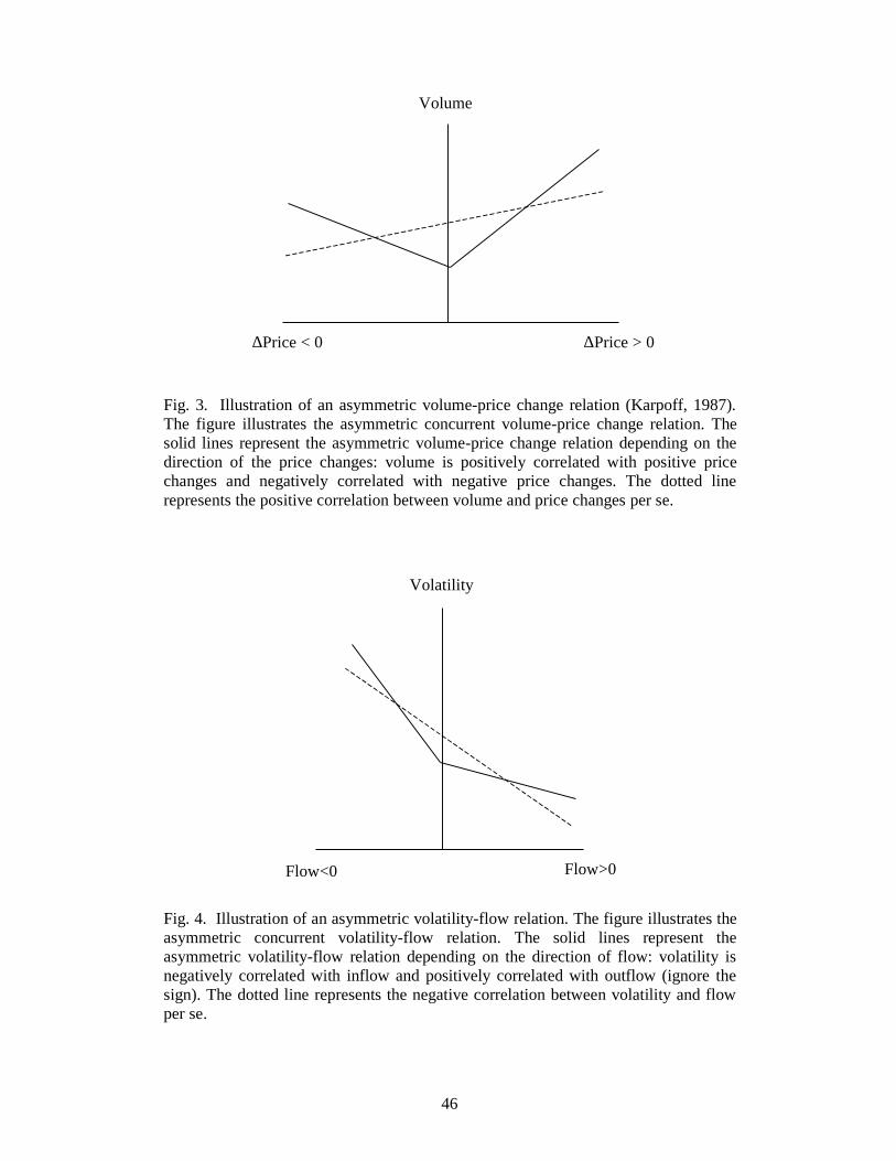
46

Fig. 3. Illustration of an asymmetric volume-price change relation (Karpoff, 1987). The figure illustrates the asymmetric concurrent volume-price change relation. The solid lines represent the asymmetric volume-price change relation depending on the direction of the price changes: volume is positively correlated with positive price changes and negatively correlated with negative price changes. The dotted line represents the positive correlation between volume and price changes per se. Fig. 4. Illustration of an asymmetric volatility-flow relation. The figure illustrates the asymmetric concurrent volatility-flow relation. The solid lines represent the asymmetric volatility-flow relation depending on the direction of flow: volatility is negatively correlated with inflow and positively correlated with outflow (ignore the sign). The dotted line represents the negative correlation between volatility and flow per se.

∆Price < 0 ∆Price > 0

Volume

Volatility

Flow>0 Flow<0