The role of credit in international business cycles

TengTeng Xu

December 2011

CWPE 1202

The role of credit in international business cycles∗

TengTeng Xu†

University of Cambridge

December 2011

Abstract

The recent financial crisis raises important issues about the role of credit

in international business cycles and the transmission of financial shocks across

country borders. This paper investigates the international spillover of US credit

shocks and the importance of credit in explaining business cycle fluctuations

using a global vector autoregressive (GVAR) model with credit, estimated over

the period 1979Q2 to 2006Q4 for 26 major advanced and emerging economies.

Results from the country-specific models reveal the importance of bank credit

in explaining output growth, changes in inflation and long term interest rates

in countries with developed banking sector. The generalized impulse response

function (GIRF) for a one standard error negative shock to US real credit provides

strong evidence of the spillover of US credit shock to the UK, the Euro area, Japan

and other industrialized economies.

Keywords: Credit, Global VAR, Macro-finance linkages, International business

cycles.

JEL Classification: C32, G21, E44, E32.

∗I am grateful to Professor M. Hashem Pesaran for his valuable guidance and continuous support.I would also like to thank Richard Louth, Kamiar Mohaddes, Alessandro Rebucci, Til Schuermann,Vanessa Smith and seminar participants at the 1st Cambridge Finance-Wharton Seminar Day, RoyalEconomic Society Easter School 2010, the 10th Econometric Society World Congress, Bank of Englandand Bank of Canada for useful discussions and helpful comments. I gratefully acknowledge financialsupport from the Overseas Research Scholarship, the Smithers & Co. Foundation and the CambridgeOverseas Trust.†Corresponding address at: Faculty of Economics, University of Cambridge, Sidgwick Avenue,

Cambridge, CB3 9DD. Email : tx204@cam.ac.uk.

1

1 Introduction

The recent credit crunch largely originated from the US housing market has led to pro-

found impact on the international financial markets as well as the global real economy.

The financial crisis and the subsequent economic downturn raises important issues on

the role of credit in international business cycles: how are credit shocks transmitted

across country borders and how important is credit in macroeconomic modeling? This

paper tries to address these questions by examining the role of credit variables using

country-specific VARX∗ models (augmented VAR with foreign variables) and study-

ing the international transmission of credit shocks using a global vector autoregressive

(GVAR) framework.

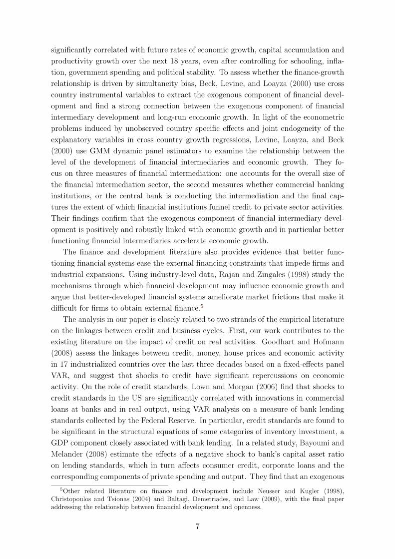
Over the past 30 years, credit has experienced steady growth in most advanced

countries and emerging economies (see Figure 1). At the same time, the globaliza-

tion of the banking sector, the increase in cross-border ownership of assets, and the

rapid development in securitization and financial engineering has increased the inter-

dependency of banking and credit markets across country borders. However, the role of

credit has been largely neglected in monetary policy making in recent decades, before

this financial crisis ignited fresh debate on this issue.1

The theoretical literature on credit market frictions has highlighted the importance

of credit, in modeling the inter-linkages between financial market and the real economy,

see for example Kiyotaki and Moore (1997), Bernanke, Gertler, and Gilchrist (1999) and

Gertler and Kiyotaki (2010). The open economy extension of this literature has shown

that credit market frictions can play an important role in transmitting shocks across

countries, through balance sheet linkages among investors and financial institutions,

see for example Devereux and Yetman (2010).

On the empirical side, many have studied the relationship between finance and

development and found better functioning financial intermediaries accelerate economic

growth, see for example Levine (2005). Some recent studies have also examined the

empirical evidence of credit channels (Braun and Larrain, 2005 and Iacoviello and

Minetti, 2008) and the impact of a US credit shock on global GDP (Helbling, Huidrom,

Kose, and Otrok, 2011). However, little empirical work has been done in quantifying

the importance of credit in explaining business cycle dynamics and in analysing the

international transmission of credit shocks in a global framework, including advanced

economies as well as emerging Asia and Latin American countries.

This paper aims to fill in the gap and the contribution in relation to the literature

is two fold: first, to my knowledge, it is the first comprehensive cross country study,

analysing and quantifying the role of credit in business cycle dynamics, for 26 major

advanced and emerging economies covering 90% of world GDP. Second, it provides

detailed analysis of the channels through which a negative shock to US real credit is

1Credit enjoyed considerable attention in monetary policy making in the 1950s and 1960s, however,its importance was replaced by a focus on money in the 1970s and part of the 1980s, before bothmoney and credit exited the main scene from late 1980s, see for example Borio and Lowe (2004).

2

transmitted across country borders and to the real economy, capturing the impact on

output, inflation and interest rates on a country by country basis.

Figure 1: Bank credit to the Private sector and Output

(log of real credit and log of real GDP in levels)

(a) United States (b) Japan

(c) Euro Area (d) UK

(e) China (f) Switzerland

The Global VAR model is estimated over the period 1979Q2 to 2006Q4, containing

26 country-specific models where the eight euro zone countries are treated as a single

economy, and including both financial and real variables in each of the country-specific

models. Among the different measures of credit, we focus on bank credit (loans and

advances) to the private sector, following the empirical literature on finance and de-

velopment where credit to the private sector is considered one of the most important

banking development indicators.

Results from the country-specific models reveal that the inclusion of credit improves

the in-sample fit of the error-correction equations in several dimensions. In particular,

3

domestic credit is found to be effective in explaining output growth, changes in inflation

and long term interest rates in countries with developed banking sector. The importance

of the credit variable in these regressions depends on the depth of the banking sector

and institutional settings of the country of interest.

The Generalized Impulse Response Functions (GIRF) for a one standard error neg-

ative shock to US real credit provide strong evidence of international spillover of US

credit shocks to the euro area, UK and Japan, with the impact on the UK particularly

profound, possibly due to the strong linkages in the banking sectors between the UK

and the US. The model predicts the spillover of credit shock to the US real economy

and its subsequent international propagation in the real sector. The US credit shock

is also accompanied by a fall in short term interest rates in the US, UK and the euro

area, suggesting a possible loosening of monetary policy in association with the con-

traction in credit availability, as observed in the policy coordination in the aftermath

of the recent credit crunch. The rapid transmission of credit shocks and the profound

impact on the international financial markets and the global real economy highlights

the important role of credit in the international business cycles.

The paper also provides strong evidence of the international spillover of shocks to US

real equity prices and oil prices. In particular, a negative shock to US real equity prices

is accompanied by a decline in real output, short term as well as long term interest rates

in the US, UK and Japan, while a positive shock to oil prices has profound impact on

real output in China and inflation in the US and the euro area.

The plan of the paper is as follows: Section 2 briefly reviews the literature on the

role of credit. Section 3 presents the GVAR methodology and the model specification.

Section 4 studies the results from the country specific VARX∗ models and evaluates the

importance of the credit variable on a country by country basis. Section 5 studies the

degree of comovements in credit compared with other business cycle variables. Section

6 presents the results from the generalized impulse response functions and discusses

their implications. Section 7 offers some concluding remarks.

2 Literature Review and Motivation

In the past decades or so, there has been rapid development in the theoretical literature

on the macroeconomic implications of financial imperfections, see for example Carl-

strom and Fuerst (1997), Kiyotaki and Moore (1997), Bernanke, Gertler, and Gilchrist

(1999) and Iacoviello (2005). By introducing credit market frictions (asymmetry of in-

formation, agency costs or collateral constraints) in dynamic general equilibrium mod-

els, research on the credit channel of monetary policy and credit cycles show that these

financial frictions act as a financial accelerator that leads to an amplification of busi-

ness cycle and highlight the mechanisms through which the credit market conditions

4

are likely to impact the real economy.2

Financial market imperfections arise from several sources: first, the asymmetry of

information between lenders and borrowers (see for example Bernanke and Gertler,

1995, Bernanke, Gertler, and Gilchrist, 1999 and Gilchrist, 2004), which induces the

lenders to engage in costly monitoring activities.3 The extra cost of monitoring by

lenders gives rise to the external finance premium of firms, which reflects the existence of

a wedge between a firm’s own opportunity cost of funds and the cost of external finance

(borrowing from the banking sector). Higher asset prices improve firm balance sheets,

reduce the external finance premium, increase borrowing and stimulate investment

spending. The rise in investment further increases asset prices and net worth, giving

rise to an amplified impact on investment and output in the economy.

Financial frictions could also stem from the lending collateral constraints faced by

borrowers (see for example Kiyotaki and Moore, 1997 and Gertler and Kiyotaki, 2010).

Credit constraints arise because lenders cannot force borrowers to repay their debts

unless the debts are secured by some form of collateral. Borrowers’ credit limits are

affected by the prices of the collateralized assets, and these asset prices are in turn

influenced by the size of the credit limits, which affects investment and demand for

assets in the economy. The dynamic interaction between borrowing limits and the

price of assets amplifies the impact of a small initial shock and generates large and

persistent fluctuations in output and asset prices in the economy.

A simple illustration of the direct relationship between credit and output can be

found in a two sector model by Biggs, Mayer, and Pick (2009), where firms cannot retain

earning in competitive product markets but must borrow entirely from the banking

sector to finance investment purchase. Under the assumption of competitive product

market, they show that output can be expressed as a function of the stock of credit

and flow of credit and suggest that credit growth has direct impact on the level of

output in the economy, with the relative importance depending on the interest rate

and depreciation rate in the economy.

In addition to the demand for credit from firms, Chen (2001) and Meh and Moran

(2004) argue that banks themselves are also subject to frictions in raising loanable funds

and show that the supply side of the credit market also contributes to shock propagation,

affecting output dynamics in the economy. In these models, moral hazard arises as the

monitoring activities of banks are not public observable–depositors are concerned that

banks may not monitor entrepreneurs adequately (so to lower the monitoring cost)

and demand that banks invest their own net worth (bank capital) in the financing of

2According to Bernanke and Gertler (1995), the credit channel is not considered as a distinct, free-standing alternative to the traditional monetary transmission mechanism, but rather a set of factorsthat amplify and propagate conventional interest rate effects of monetary policy. Financial frictionsare essential in propagating financial shocks to the real economy. Modigliani and Miller (1958) theoremimplies that, without financial frictions, leverage or financial structure is irrelevant to real economicoutcomes.

3For example, costly state verification, first introduced in Townsend (1979) and further developedin Bernanke, Gertler, and Gilchrist (1999).

5

entrepreneurial projects. The extra financial friction between banks and their depositors

constrain the supply of credit and hence the leverage of entrepreneurs in the economy.4

Several studies apply models of financial frictions to an open economy to explore the

role of financial markets in the international transmission mechanism. Devereux and

Yetman (2010) study the international transmission of shocks due to interdependent

portfolio holdings among leverage-constrained investors and highlight the importance of

balance sheet linkages among investors and financial institutions across countries. They

develop a two country model in which investors borrow from savers and invest in fixed

assets. Investors also diversify their portfolios across countries and hold equity positions

in the assets of the other country in addition to their own. When leverage constraints

are binding, a fall in asset values in one country forces a large and immediate process of

balance sheet contractions for that country’s investor, similar to the process outlined in

Kiyotaki and Moore (1997). More importantly, the asset price collapses are transmitted

internationally through deterioration in the balance sheets of institutions in countries

holding portfolios of similar assets. The final result is a magnified impact of the initial

shock, a large fall in investment and output, and highly correlated business cycle across

countries during the downturn. Other notable papers on financial frictions in an open

economy include Gilchrist (2004), who focuses on the asymmetries between lending

conditions across economies, using the external finance premium model developed in

Bernanke, Gertler, and Gilchrist (1999). Gilchrist (2004) predicts that highly leverage

countries (where the share of investment financed through external funds is high) are

more vulnerable to external shocks, owing to their effect on foreign asset valuations and

thus on borrower net worth.

Another important area of theoretical literature examines the spillover of shocks in

an open economy through trade linkages. Trade linkages play an important role since

the slowdown in output (as a result of a credit shock) is largely transmitted through

trade across country borders. Backus, Kehoe, and Kydland (1994) and Kose and Yi

(2006) model a particular type of trade linkage between countries, where final goods are

produced by combining domestic and foreign intermediate goods. In their framework,

an increase in final demand leads to an increase in demand for foreign intermediates,

which results in a transmission of shocks to the foreign country.

On the empirical side of the literature, many have studied the linkages between

finance and development, see for example the survey papers by Levine, Loayza, and

Beck (2000) and Levine (2005). The finance and development literature provides strong

evidence that countries with more fully developed financial systems tend to grow faster,

in particular those with large, privately owned banks that channel credit to private en-

terprises and liquid stock exchanges. For example, using cross-country studies, Levine

and Zervos (1998) find that the initial level of banking development are positively and

4Other work that focus on the role of the banking sector include Christiano, Motto, and Rostagno(2008), Freixas and Rochet (2008), Goodhart, Sunirand, and Tsomocos (2004), Goodhart, Sunirand,and Tsomocos (2005) and de Walque, Pierrard, and Rouabah (2009), with the latter three studyingthe role of banking sector in financial stability.

6

significantly correlated with future rates of economic growth, capital accumulation and

productivity growth over the next 18 years, even after controlling for schooling, infla-

tion, government spending and political stability. To assess whether the finance-growth

relationship is driven by simultaneity bias, Beck, Levine, and Loayza (2000) use cross

country instrumental variables to extract the exogenous component of financial devel-

opment and find a strong connection between the exogenous component of financial

intermediary development and long-run economic growth. In light of the econometric

problems induced by unobserved country specific effects and joint endogeneity of the

explanatory variables in cross country growth regressions, Levine, Loayza, and Beck

(2000) use GMM dynamic panel estimators to examine the relationship between the

level of the development of financial intermediaries and economic growth. They fo-

cus on three measures of financial intermediation: one accounts for the overall size of

the financial intermediation sector, the second measures whether commercial banking

institutions, or the central bank is conducting the intermediation and the final cap-

tures the extent of which financial institutions funnel credit to private sector activities.

Their findings confirm that the exogenous component of financial intermediary devel-

opment is positively and robustly linked with economic growth and in particular better

functioning financial intermediaries accelerate economic growth.

The finance and development literature also provides evidence that better func-

tioning financial systems ease the external financing constraints that impede firms and

industrial expansions. Using industry-level data, Rajan and Zingales (1998) study the

mechanisms through which financial development may influence economic growth and

argue that better-developed financial systems ameliorate market frictions that make it

difficult for firms to obtain external finance.5

The analysis in our paper is closely related to two strands of the empirical literature

on the linkages between credit and business cycles. First, our work contributes to the

existing literature on the impact of credit on real activities. Goodhart and Hofmann

(2008) assess the linkages between credit, money, house prices and economic activity

in 17 industrialized countries over the last three decades based on a fixed-effects panel

VAR, and suggest that shocks to credit have significant repercussions on economic

activity. On the role of credit standards, Lown and Morgan (2006) find that shocks to

credit standards in the US are significantly correlated with innovations in commercial

loans at banks and in real output, using VAR analysis on a measure of bank lending

standards collected by the Federal Reserve. In particular, credit standards are found to

be significant in the structural equations of some categories of inventory investment, a

GDP component closely associated with bank lending. In a related study, Bayoumi and

Melander (2008) estimate the effects of a negative shock to bank’s capital asset ratio

on lending standards, which in turn affects consumer credit, corporate loans and the

corresponding components of private spending and output. They find that an exogenous

5Other related literature on finance and development include Neusser and Kugler (1998),Christopoulos and Tsionas (2004) and Baltagi, Demetriades, and Law (2009), with the final paperaddressing the relationship between financial development and openness.

7

fall in bank capital/asset ratio by one percent point reduces real GDP by some one and

a half percent through its effects on credit availability. Development in the theoretical

literature on the credit channel of monetary policy has sparked interests in examining

the empirical evidence of credit channels, see for example Braun and Larrain (2005)

and Iacoviello and Minetti (2008). Using micro data on manufacturing industries in

more than 100 countries during the last 40 years, Braun and Larrain (2005) find strong

support for the existence of the credit channel and show that industries that are more

dependent on external finance are hit harder during recessions and countries with poor

accounting standards (a proxy for information asymmetries and financial frictions) and

highly dependent industries experience more severe impact during economic downturns.

The existing empirical literature on the linkages between credit and real activities

has largely focused on the impact of credit on output dynamics, while little has been

done in analysing the effect of credit on inflation, short term and long run interest rates

in the economy, nor in quantifying the importance of credit in the macroeconomy, both

of which we aim to address in our paper.

Secondly, our paper is closely related to the latest research on the international

transmission of credit shocks. For example, Galesi and Agherri (2009) examine the

transmission of regional financial shocks in Europe using a Global VAR framework. The

model is estimated for 26 European economies and the US and they find that asset prices

are the main channel through which financial shocks are transmitted internationally,

at least in the short run, whereas the contribution of other variables, including the

cost and quantity of credit only become important over longer horizons. Their analysis

focuses on regional spillovers in Europe, in particular between advanced and emerging

European economies, while we are more interested in the interactions in the world

economy, where emerging Asia and oil-producing countries are increasingly playing

an important role. Helbling, Huidrom, Kose, and Otrok (2011) examine the impact

of global credit shocks on global business cycles, using global factors of credit, GDP,

inflation and interest rates, constructed with data from G-7 countries. They also study

the impact of a US credit shock using a FAVAR (factor augmented VAR) model on US

GDP and the global factor of GDP and find that the US credit market shocks have a

significant impact on the evolution of global growth during the recent financial crisis.

While this paper sheds some light on the impact of a US credit shock on the global

factor of GDP, it has not examined the mechanism through which US credit shock is

transmitted to individual emerging economies and advanced countries, accounting for

the differences in responses among countries. Finally, Cetorelli and Goldberg (2008,

2010) show that global banks played a significant role in the transmission of liquidity

shocks through a contraction in the cross border lending. However, this line of research

has not considered the impact of liquidity shocks on the real economy and the resulting

propagation into the real sector.

As we can see, the existing literature on the international transmission of credit

shocks has not examined the transmission of US credit shocks to both advanced and

8

emerging economies and the subsequent impact on the real economy including output,

inflation and interest rates on a country by country basis. Our paper aims to fill in

the gap and offers a comprehensive analysis of the channels through which a US credit

shock is transmitted to advanced economies as well as emerging Asia, Latin America

and oil-producing countries and compares its impact with other financial shocks, such

as shocks to US real equity and oil prices.

3 Methodology

3.1 The GVAR approach

The theoretical insights and the existing empirical literature suggest that there could

be important linkages between bank credit and business cycle dynamics. To study the

spillover of credit shocks across country borders and its impact on the real economy, we

incorporate bank credit in a global VAR framework, pioneered in Pesaran, Schuermann,

and Weiner (2004) (hereafter PSW) and further developed in Pesaran and Smith (2006),

Dees, di Mauro, Pesaran, and Smith (2007) (hereafter DdPS), Dees, Holly, Pesaran,

and Smith (2007) (hereafter DHPS). The GVAR model is a multi-country framework

which allows for the analysis of the international transmission mechanics and the in-

terdependencies among countries.

Following PSW and DdPS, suppose there are N + 1 countries (or regions) in the

global economy, indexed by i = 0, 1, ..., N , where country 0 is treated as the reference

country (which we take as the US in this case). The individual country VARX∗(pi, qi)

model for the ith economy can be written as:6

Φi(L, pi)xit = ai0 + ai1t+ Υi(L, qi)dt + Λi(L, qi)x∗it + uit, (1)

for i = 0, 1, ..., N , where xit is the ki × 1 vector of domestic variables (including, for

example, real GDP, inflation, interest rates and real credit), x∗it is the k∗i × 1 vector

of country-specific foreign variables, dt denotes the md × 1 matrix of observed global

factors, which could include international variables such as world R&D expenditure, oil

or other commodity prices, ai0 and ai1 are the coefficients of the deterministics, here

intercepts and linear trends, and uit is the idiosyncratic country specific shock. Further,

we have Φi(L, pi) =∑pi

l=0 ΦilLl, Υi(L, qi) =

∑qim=0 ΥimL

m, Λi(L, qi) =∑qi

n=0 ΥinLn,

where L is the lag operator and pi and qi are the lag order of the domestic and foreign

variables for the ith country.

Country specific VARX∗ models are vector autoregression models augmented with

country-specific foreign variables x∗it, constructed using trade weights wij, j = 0, 1, ...., N ,

6DdPS develop a theoretical framework where the GVAR is derived as an approximation to a globalunobserved common factor model.

9

that capture the importance of country j for country i’s economy

x∗it =N∑j=0

wijxjt, (2)

where wii = 0 and∑N

j=0 wij = 1,∀i, j = 0, 1, ...., N . The weights wij are estimated

by bilateral trade data drawn from the IMF Direction of Trade Statistics, where wij

captures the importance of country j for country i ’s economy in the share of exports

and imports. We first use fixed weights based on the average trade flows computed

over the three years 2001 to 2003, we could later allow time-varying trade weights in

our analysis.

Trade weights are considered our preferred measure of weights in the GVAR for

three main reasons. Firstly, trade is found to be the most important determinants of

cross country linkages and international business cycle synchronization, see for example

Forbes and Chinn (2004), Imbs (2004), Baxter and Kouparitsas (2005) and Kose and Yi

(2006). Baxter and Kouparitsas (2005) study the determinants of international business

cycle comovements and conclude that bilateral trade is the most important source of

inter-country business cycle linkages. Imbs (2004) provides further evidence on the

effect of trade on business cycle synchronization and concludes that while specialization

patterns have a sizable effect on business cycles, trade continues to play an important

role in this process. Focusing on global linkages in financial markets, Forbes and Chinn

(2004) also show that direct trade appears to be one of the most important determinants

of cross-country linkages.

Secondly, time series on bilateral trade data are also more readily available for

developing or emerging market economies, as compared to data on bilateral financial

flows. For example, the International banking statistics published by the BIS and the

Bilateral FDI data published by the OECD do not provide data on bilateral financial

flows between developing countries.7 The lack of available bilateral financial flow data

among emerging economies means that these financial weights are not likely to fully

capture the interlinkages between the 15 developing countries modeled in the GVAR

and to reveal the full extent of globalization. For example, should we use financial

weights as the aggregation weights, a weight of zero will be assigned to the bilateral

linkage between China and Brazil due to data availability, which does not reflect the

important trade linkages between these two countries (according to IMF Direction of

7International banking statistics from the Bank for International Settlements (BIS) measure consol-idated foreign claims of reporting banks on individual countries (through both direct lending and localbanking systems). The countries that report the consolidated banking statistics to the BIS comprisethe largest international banking centers. For the 33 countries considered in the GVAR, only 20 wereamong the reporting countries. The OECD International Direct Investment Database (Source OECD)publish data on bilateral FDI flows (inflows and outflows) among OECD and non-OECD countriesover the period from 1985 to 2006, in particular FDI outflows from OECD countries to all countries,as well as FDI outflows from non OECD countries to OECD countries, but not FDI outflows from nonOECD to non OECD countries

10

Trade Statistics, China accounts for around 10% of total trade in Brazil in 2005).8

Furthermore, due to the generally high cross country correlation of variables such

as output or real equity prices, mis-specification of the weights might not have strong

implication for the measurement of foreign variables. Asymptotic results suggest that

the type of aggregate weights used would not be important if there was a strong common

factor among the country series. Finally, it is important to note that international

financial linkages have already been captured in our modeling framework, through the

inclusion of country specific foreign financial variables, such as equity, credit and long

run interest rates.

For each country model, we consider at most a VARX∗(2, 2) specification9

xit = ai0 + ai1t+ Θi1xi,t−1 + Θi2xi,t−2 + Υi0dt + Υi1dt−1 + Υi2dt−2

+Λi0x∗it + Λi1x

∗i,t−1 + Λi2x

∗i,t−2 + uit.

The corresponding error correction term may be written as

∆xit = ci0−αiβ′i[ζi,t−1−γi(t−1)]+Υi0∆dt+Λi0∆x∗it+Υi1∆dt−1 +Γi∆zi,t−1 +uit, (3)

where zit = (x′it,x∗′it )′, ζi,t−1 = (z′i,t−1,d

′i,t−1)′, αi is a ki × ri matrix of rank ri, βi

is a (ki + k∗i + md) × ri matrix of rank ri (the number of cointegration relationships

in the system). We could further partition β′i as βi = (β′ix, β′ix∗ , β

′id)′ conformable to

ζit = (x′it,x∗′it ,d

′t)′, and the ri error correction terms defined above can be written as

β′i(ζit − γit) = β′ixxit + β′ix∗x∗′it + β′idd

′t − (β′iγi)t,

which allows for the possibility of cointegration within xit, between xit and x∗it and

across xit and xjt for i 6= j. Notice that the coefficient of the linear trend in the

error correction form is restricted (αiβ′iγi), to avoid the possibility of quadratic trend in

xit and to ensure that the deterministic trend property of the country-specific models

remains invariant to the cointegrating rank assumptions, see Pesaran, Shin, and Smith

(2000).

An important condition in the GVAR framework is the weak exogeneity of the

foreign variables, which implies that there is no long run feedback from xit to x∗it,

without necessarily ruling out lagged short run feedback between xit and x∗it. That is,

8Several studies have explored the possibility of using different weights to construct country-specificforeign variables, for example, Hiebert and Vansteenkiste (2007) use weights based on the geographicaldistances among region, Vansteenkiste (2007) adopts weights based on sectorial input-output tablesacross industries and Galesi and Agherri (2009) construct financial weights based on the consolidatedforeign claims of reporting banks on individual countries in the BIS International banking statistics.However, these studies mainly focus on linkages between developed economies or between developedand developing economies, a weight of zero is imposed for bilateral financial flows among developingcountries where data is not available.

9DHPS consider a VARX∗(2, 1) specification across all countries and PSW consider a VARX∗(1, 1)specification.

11

the domestic economic conditions cannot affect the ‘the rest of the world’ in the long

run, though there can be short run interactions between the two set of variables. In

effect, each country is treated as a small open economy in the framework except for

the US. The weak exogeneity assumption is later tested by examining the significance

of the error correction terms of the individual country vector error correction models

in the marginal error correcting model of x∗it.

After estimating each country VARX∗ model, all the k =∑N

i=0 ki endogenous vari-

ables are collected in the k × 1 global vector xt = (x′0t,x′1t, ...,x

′Nt)′ and solved si-

multaneously using link matrix defined in terms of the country specific weights. De-

note zit = (xt,x∗t )′ a vector of domestic and foreign variables, then the individual

VARX∗(pi, qi) model in Equation (1) can be written as

Ai(L, pi, qi)zit = ϕit, i = 0, 1, 2, ..., N, (4)

where

Ai(L, pi, qi) = [Φi(L, pi),−Λi(L, pi)],

ϕit = ai0 + ai1t+ Υi(L, qi)dt + uit.

The vector zit can be written as

zit = Wixt, i = 0, 1, 2, ..., N, (5)

where Wi is a link matrix of dimension (ki + k∗i ) × k, constructed based on country

specific weights. Substitute (5) into (4), we have

Ai(L, pi, qi)Wixt = ϕit, i = 0, 1, 2, ..., N. (6)

The vector of endogenous variables of the global economy, xt, can now be obtained

by stacking the country specific models (6) as

G(L, p)xt = ϕt, (7)

where

G(L, p) =

A0(L, p)W0

A1(L, p)W1

...

AN(L, p)WN

, ϕt =

ϕ0t

ϕ1t

...

ϕNt

,

and p = max(p0, p1, ..., pN , q0, q1, ..., qN). The model in (7) is a high dimensional VAR

model which can be solved recursively, and used for generalized impulse response anal-

ysis and forecasting.

12

3.2 The GVAR model with credit

The version of the GVAR model developed in this paper covers 33 countries, where 8 of

the 11 countries that originally joined the euro on 1 January 1999 (Austria, Belgium,

Finland, France, Germany, Italy, Netherlands and Spain) are aggregated using the

average Purchasing Power Parity GDP weights, computed over the 2001-2003 period.

In effect, we consider a global model with 26 advanced and emerging market economies

(accounting for 90% of world output), estimated over the period 1979Q2 to 2006Q4.

The choice of the credit measure used in this paper “bank credit (loans and ad-

vances) to the private sector” is guided by the existing literature, data availability and

the consideration of international comparability across country series. First, banking

sector refers to deposit money banks, which comprise commercial banks and other fi-

nancial institutions that accept transferable deposits, such as demand deposits. They

often engage in core banking services that extend loans to the non-financial corpora-

tions, which ultimately determine the level of investment and output in the economy.

Second, we focus on credit to the private sector, following the empirical literature on

finance and development, where credit to the private sector is considered the most im-

portant banking development indicator, since it proxies the extent to which new firms

have opportunities to obtain bank finance and this in turn could influence short term

fluctuations in the level of output and economic growth in the economy.10 Third, we

choose to use the level of ‘claims on private sector from deposit money banks’ rather

than its ratio to GDP, as seen in the finance and development literature.11 The rea-

son is that our objective is not to study the extent of financial intermediation in the

economy but the overall level of bank credit that is available to the private sector.

The source of credit data for all countries, except UK, Australia and Canada, was

the series ‘Claims on Private Sector from Deposit Money Banks’ (22d) from the IFS

Money and Banking Statistics, measured in national currency in current prices. The

data source for the UK and Australia was the National Statistics from Datastream

and for Canada was the OECD data from Datastream. The data series on the other

variables are drawn from the rejoinder in Pesaran, Schuermann, and Smith (2009),

which covers the period 1979Q1 to 2006Q4.12

Many of the IMF credit series displayed large level shifts due to changes in the

definition and re-classifications of the banking institutions. Following Goodhart and

Hofmann (2008) and Stock and Watson (2003), we adjust for these level shifts by

replacing the quarterly growth rate in the period when the shift occurs with the median

10See for example Levine, Loayza, and Beck (2000) and Baltagi, Demetriades, and Law (2008).11 For example, King and Levine (1993a,b) use the ratio of gross claims on the private sector to

GDP in their study. Levine and Zervos (1998) and Levine (1998) use the ratio of deposit money bankcredit to the private sector to GDP over the period 1976 to 1993. Levine, Loayza, and Beck (2000)use a measure of private credit as an indicator of financial intermediary development from 1960 to1995, where Private credit equals the ratio of credits by financial intermediaries to the private sectorto GDP.

12The data set in the rejoinder of Pesaran, Schuermann, and Smith (2009) is a revised and extendedversion of the data set used in DdPS, which ends in 2003Q4.

13

Table 1: Countries/Regions included in the GVAR

United States Euro Area Latin AmericaChina Germany BrazilJapan France MexicoUnited Kingdom Italy Argentina

Spain ChileCanada Netherlands PeruAustralia BelgiumNew Zealand Austria

Finland

Rest of Asia Rest of W. Europe Rest of the WorldKorea Sweden IndiaIndonesia Switzerland South AfricaThailand Norway TurkeyPhilippines Saudi ArabiaMalaysiaSingapore

of the growth rate of the two periods prior and after the level shift. The level of the

series is then adjusted by backdating the series based on the adjusted growth rates. The

nominal credit series are deflated by the CPI to obtain the real credit series, which are

seasonally adjusted where necessary, according to the combined test for the presence

of identifiable seasonality.13

We include real output (yit), the rate of inflation (πit = pit−pi,t−1), the real exchange

rate (eit − pit), real equity prices (qit), real credit (crdit), the short term interest rate

(ρSit) and the long rate of interest (ρLit) in the GVAR, where available. More specifically

yit = ln(GDPit/CPIit), pit = ln(CPIit), eit = ln(Eit),

crdit = ln(CRDit/CPIit), qit = ln(EQit/CPIit),

ρSit = 0.25× ln(1 +RSit/100), ρLit = 0.25× ln(1 +RL

it/100),

where GDPit is the nominal Gross Domestic Product, CPIit the consumer price index,

EQit the nominal equity price index, CRDit the nominal credit, Eit the exchange rate

in terms of US dollars, RSit is the short term interest rate, and RL

it the long rate of

interest, for country i during the period t.

In order to verify to what degree the credit series have univariate integration proper-

ties, we perform the unit root tests over the sample period for the levels and first differ-

ences of the logarithm of real credit (after seasonality adjustment) for the 33 countries

considered in the GVAR.14 ADF tests and the weighted symmetric estimation of the

ADF type regressions (introduced by Park and Fuller, 1995) in general support the view

13A detailed discussion on the choice of credit variable, a comparison between the IFS and Datas-tream data source, adjustment for level shifts and seasonality can be found in Appendix A.

14According to Dickey and Pantula (1987), the appropriate sequence of testing for unit root is tofirst check whether the variables are stationary in their first differences.

14

that credit variables are integrated of order one. DdPS noted that the weighted sym-

metric (WS) tests exploit the time reversibility of stationary autoregressive processes

and hence possess higher power compared with the traditional Dickey-Fuller (DF) tests.

Further, Pantula, Gonzalez-Farias, and Fuller (1994) and Leybourne, Kim, and New-

bold (2005) provide evidence of superior performance of the weighted symmetric (WS)

test statistics compared with the standard ADF tests or the GLS-ADF tests (Elliott,

Rothenberg, and Stock, 1996). The test results also support the unit root properties of

the other variables considered in the GVAR and we consider the key variables including

credit as I(1) in our empirical analysis hereafter, since it allows the empirical model to

adequately represent the statistical features of the series over the sample period and

provides the scope for studying long run structural relationships in the model.15

With the exception of the US model, all country specific models include yit, πit,

ρSit, ρLit, qit, crdit and eit − pit as domestic variables, where available, and their foreign

counterparts y∗it, π∗it, q

∗it, ρ

∗Sit , ρ

∗Lit , crd

∗it as country-specific foreign variables, excluding ex-

change rate, which is already determined in the model, and including the log of oil prices

(pot ), as given in Table 2.

Table 2: Model specifications

Country Domestic variables Foreign variables

US yit, ∆pit, ρSit, ρ

Lit, qit, crdit, p

ot y∗it, ∆p∗it, ρ

S∗

it , e∗it − p∗it

Rest of yit,∆pit, ρSit, ρ

Lit, qit, crdit, eit − pit y∗it,∆p

∗it, ρ

S∗

it , ρL∗

it , q∗it, crd

∗it, p

ot

the world where available

The US is considered the dominant economy in the model, and the specifications for

the US model differ accordingly. Oil prices are included as an endogenous variable in the

US model, to allow for macro variables to influence the evolution of oil prices. Given the

importance of the US financial variables in the global economy, the US-specific foreign

financial variables q∗US,t, ρ∗LUS,t, crd

∗US,t were not included in the US model as they were not

long run forcing (weakly exogenous) with respect to the US domestic financial variables,

see below for supporting test results. The US-specific foreign output, inflation, short

term interest rate and exchange rate variables y∗it, π∗it, ρ

∗SUS,t and e∗US,t − p∗US,t were

included in the US model in order to capture the possible second round effects of

external shocks on the US, and as we shall see below they do satisfy the weak exogeneity

assumption.

As mentioned earlier, one important condition underlying the GVAR estimation

strategy is the weak exogeneity of x∗it with respect to the long-run parameters of the

conditional model. Weak exogeneity is tested along the lines described in Johansen

(1992) and Harbo, Johansen, Nielsen, and Rahbek (1998). This involves a test of the

joint significance of the estimated error correction term in auxiliary equations for the

15Please see Appendix B for detailed results on unit root testing.

15

country-specific foreign variables, x∗it. In particular, for each lth element of x∗it the

following regression is carried out:

∆x∗it,l = µil +

ri∑j=1

γij,lECMji,t−1 +

si∑k=1

ϕik,l∆xi,t−k +

ni∑m=1

ϑim,l∆x̃∗i,t−m + εit,l, (8)

where ECM ji,t−1, j = 1, 2, ..., ri, are the estimated error correction terms corresponding

to the ri cointegrating relations found for the ith country model and ∆x̃∗i,t= (∆x′∗i,t,

∆(e∗it − p∗it), ∆p0t )′. In the case of the USA the term ∆(e∗it − p∗it) is implicitly included

in x∗i,t. The test for weak exogeneity is an F-test of the joint hypothesis that γij,l =

0, j = 1, 2, ...ri, in the above regression. In this case, we take the lag orders si to be

the same as the orders pi of the underlying country-specific VARX* models and the lag

orders ni to be two. We find that the weak exogeneity hypothesis could not be rejected

for the majority of the variables being considered, especially for core economies such

as the US, the euro area, UK and China.16

Table 3: F-statistics for testing the weak exogeneity of the country-specificforeign variables and oil prices–selected countries

Country Foreign variables

y∗t ∆p∗t q∗t ρS∗

t ρL∗

t crd∗t pot e∗t − p∗t

US F( 2,83) 0.143 1.309 1.247 2.57UK F( 3,74) 0.409 0.774 0.125 0.135 0.056 2.532 0.397

Euro Area F( 3,72) 0.187 2.495 1.710 2.726 0.898 1.408 1.305Switzerland F( 3,74) 0.154 0.2 1.163 0.199 0.59 1.668 2.778

Japan F( 4,73) 0.597 0.991 0.71 1.761 1.336 0.233 1.832China F( 2,79) 1.953 1.351 0.378 0.126 0.312 1.508 1.517India F( 1,78) 0.039 0.111 1.433 0.028 0.375 0.022 0.011Brazil F( 2,79) 0.242 1.957 1.703 2.258 0.843 3.664† 0.582

Note: These F statistics test zero restrictions on the coefficients of the error correction terms in the error-correction regression for the country-specific foreign variables. ‘†′ indicates significance at 5% level. Thelag orders of the VARX∗ models used for the weak exogeneity tests are set as follows: the lag order for thedomestic variable is equal to the that in the GVAR model selected by AIC, the lag order for the foreignvariables is set to be two for all countries except the euro zone where we use the lag order 4, since there wasserial correlation in several of the regression equations with lower order.

4 The Role of Credit in Country Specific Models

The theoretical literature on the role of credit (see details in the literature review)

has highlighted the importance of credit in real economic activities. To examine and

quantify the importance of credit in modeling output growth, changes in inflation, in-

terest rates, exchange rates, equity prices and oil prices, we estimate country specific

VARX∗ models for 26 advanced and emerging economies, based on the error correction

16Please see Table 3 for the test results or the weak exogeneity hypothesis for the core economies,the test statistics for the remaining countries can be found in Table C1 in the appendix.

16

model representation specified in equation (3) and taking into account of the long run

relationships between financial and real variables and between domestic and country

specific foreign variables. In order to evaluate the in-sample performance of the credit

models (i.e. error correction models with real credit), we compare their in sample fit

with two benchmark models. The first of which captures an otherwise identical error

correction model except for the exclusion of the variable real credit (crdt), while the

second benchmark is estimated as an AR(p) specification applied to the first differ-

ence of each of the seven core country-specific endogenous variables in turn, with the

appropriate lag order p selected by the Akaike information Criteria.17

4.1 Lag order and number of cointegration relationships

The country specific models are estimated by first selecting the appropriate lag order

and the number of cointegration relationships in each of the country specific models.

We select the lag order of the domestic variables pi according to the Akaike information

criterion and we set the lag order of the foreign variables, qi to be one in all countries

with the exception of UK, where Akaike information criterion favours a VARX∗(2, 2).

Owing to data limitations, we do not allow pmax or qmax to be greater than two, but

a VARX∗ in 7 variables is capable of generating quite rich dynamics at the level of

individual variables.

After selecting the appropriate lag order for the individual VARX∗ model with

unrestricted intercepts and restricted trend coefficients, we compute Johansen’s ‘trace’

and ‘maximal eigenvalue’ statistics.18 As shown by Cheung and Lai (1993) using Monte

Carlo experiments, the maximum eigenvalue test is generally less robust to the presence

of skewness and excess kurtosis in the errors than the trace tests. Given that we have

evidence of non-normality in the residuals of the VARX∗ model used to compute the test

statistics (due to the inclusion of variables such as equity prices and interest rates, all

of which exhibit significant degrees of departure from normality), we therefore believe

it more appropriate to base our cointegration tests on the trace statistics. The selected

lag orders and the number of cointegration relationships by country are given in the

Table 4.

4.2 Parameter estimates and error correction equations

Once the appropriate lag order and the number of cointegration relationships are spec-

ified, the next stage in the estimation is to exactly identify the long run, which with

n cointegration relations require n2 restrictions. DdPS argue that in one sense, the

choice of the exactly identifying restrictions is arbitrary, since the maximized value of

17The a priori maximum lag order for the autoregressive process is set as four.18We selected a VARX∗ with unrestricted intercepts and restricted trends since the variables con-

sidered are trended and we wish to avoid the possibility of quadratic trends in some of the variables,see for example PSW for detailed mathematical exposition.

17

the log-likelihood function is identical under an alternative exactly identified scheme.

In another sense, however, the choice of exactly identifying restrictions is crucial, as

it provides the basis for the development of an econometric model with economically

meaningful long-run properties. It is therefore important that the cointegrating rela-

tions are exactly identified by imposing restrictions that are a subset of those suggested

by economic theory. It is also good practice to avoid using doubtful theory restrictions

as exact identifying restrictions. For example, for the US with a VARX∗(2,1) speci-

fication with two cointegration relationships, economic theory and the coefficients in

the cointegration vectors obtained under Johansen’s just-identifying restrictions sug-

gest that Fisher equation and the term structure of interest rate are the two long run

relationships relevant to our model:

ρSit −∆pit ∼ I(0),

ρSit − ρLit ∼ I(0).

We impose four exact identifying restrictions, on the coefficients of short term interest

rate and inflation in the first cointegrating vector and on short term and long term inter-

est rates in the second cointegrating vector. Using the above exactly identified model,

we can also test for the over-identifying restrictions, including the co-trending hypothe-

sis, the Fisher equation and the term structure of interest rate relationships for the US

model. In the current version of the paper, we focus on the case of exact-identifying

restriction and we do not impose over-identifying restriction on the cointegration rela-

tions.

4.2.1 The United States

Following a VARX∗(2,1) specification with two cointegration relationships, the short run

dynamics of the US model are characterized by the seven error correction specifications

given in Table 5. The estimates of the error correction coefficients show that the long

run relations make an important contribution in several equations and that the error

correction terms provide for a complex and statistically significant set of interactions

and feedbacks across output, inflation and credit equations. The credit variable is

significant in explaining output and credit growth and changes in the short term interest

rate. The results in Table 5 also show that the core model fits the historical data well,

especially for the US output, inflation, short term interest rate and credit equation.

In comparison the benchmark models, we find that, the inclusion of credit improves

the fit for the output and oil price equation. In particular, the adjusted R2 rises

from 0.488 to 0.571 in the output equation with the inclusion of credit. Our result is

consistent with the existing empirical literature, for example Bayoumi and Melander

(2008) have also found important empirical evidence on US Macro-financial linkages

through the role of credit and bank capital adequacy. The core model with credit

outperforms the AR benchmark in the case of all variables except for oil prices and the

18

Table 4: VARX∗ order and number of cointegration relationships in thecountry-specific models

VARX∗(pi, qi) No. of VARX∗(pi, qi) No. ofCountry pi qi CR Country pi qi CR

China 2 1 2 Malaysia 1 1 1Euro Area 2 1 3 Philippines 2 1 2

Japan 2 1 4 Singapore 1 1 3Argentina 2 1 3 Thailand 1 1 2

Brazil 2 1 2 India 2 1 1Chile 2 1 3 South Africa 2 1 3

Mexico 2 1 4 Saudi Arabia 2 1 1Peru 2 1 3 Turkey 2 1 2

Australia 2 1 3 Norway 2 1 4Canada 2 1 4 Sweden 2 1 3

New Zealand 2 1 3 Switzerland 2 1 3Indonesia 2 1 3 UK 2 2 3

Korea 2 1 4 US 2 1 2

Note: The lag orders of the VARX∗ models are selected by AIC. The number of cointegrationrelationships are based on trace statistics with MacKinnon’s asymptotic critical values. To resolvethe issues of potential overestimation of cointegration relationships with asymptotic critical values,we reduce the number of cointegration relationships for six countries, as marked in bold, to beconsistent to economic theory and to maintain the stability in the global model.

credit variable.

4.2.2 The Euro Area

Recall that the euro area economies (Austria, Belgium, Finland, France, Germany, Italy,

Netherlands and Spain) are aggregated using the average Purchasing Power Parity GDP

weights, computed over the 2001-2003 period. Similar to the US model, we consider a

VARX∗(2,1) model for our analysis.

The error-correction model under the exactly-identified restrictions suggest that the

core model with credit fits historical data well, especially for the output, inflation, equity

and long run interest rate equation in the euro area. Bank credit plays a particular

important role in explaining real activities in the euro area since loans (bank finance)

are by far the most important source of debt financing of non-financial corporations

in the euro area, in comparison to the US (see for example Ehrmann, Gambacorta,

Martinez-Pages, Sevestre, and Worms, 2001).

The explanatory power of the equity equation for the euro area seems unreasonably

high in first instance (R̄2=0.83), after re-estimating the model with different subset

of the variables, we identify that it is foreign equity that contributes most to the R̄2

for the equity equation, which is in line with the high level of international spillover

in the equity market. The diagnostics statistics of the equations are generally satis-

factory as far as the tests of serial correlation, functional form and heteroscedasticity

are concerned. The assumption of normally distributed errors is rejected in the short

term interest rate equation, which is understandable if we consider the major hikes in

19

Table 5: In sample fit and Diagnostics for the US core model, USVARX∗(2,1) model

Equation ∆yt ∆(∆pt) ∆qt ∆ρSt ∆ρLt ∆crdt ∆pot∆yt−1 -0.112 −0.185† 2.005 -0.004 -0.011 -0.084 -1.445

(0.093) (0.082) (1.240) (0.033) (0.023) (0.188) (2.579)∆(∆pt−1) 0.072 0.267† -1.806 −0.133† -0.019 0.246 0.984

(0.126) (0.111) (1.689) (0.045) (0.256) (3.514)∆qt−1 0.013 0.019† 0.137 0.006∗ 0.004† −0.032∗ 0.355

(0.008) (0.007) (0.110) (0.003) (0.002) (0.017) 0.229∆ρSt−1 1.626† 0.253 -1.585 -0.041 -0.145 -0.423 -13.215

(0.387) (0.341) (5.181) (0.139) (0.097) (0.786) (10.781)∆ρLt−1 −0.951∗ 1.246† -11.197 0.253 0.272† −1.809∗ 31.051†

(0.522) (0.460) (6.980) (0.188) (0.131) (1.059) (14.523)∆crdt−1 0.143† -0.058 0.407 0.026∗ -0.006 0.702† 1.645

(0.043) (0.038) (0.576) (0.015) (0.011) (0.087) (1.199)∆pot−1 -0.004 -0.002 0.003 0.003† 0.0008 0.009 0.111

(0.004) (0.003) (0.053) (0.001) (0.001) (0.008) (0.110)∆y∗t 0.712† 0.125 -2.454 0.142† 0.139† 0.591† 5.558

(0.127) (0.112) (1.699) (0.046) (0.032) (0.258) (3.535)∆(∆p∗t ) 0.189∗ 0.213† 1.307 -0.018 0.028 −0.358∗ -1.163

(0.097) (0.086) (1.301) (0.035) (0.024) (0.197) (2.707)

∆ρS∗

t 0.218 -0.027 −3.201∗ 0.036 -0.038 0.290 6.512∗

(0.132) (0.116) (1.760) (0.047) (0.033) (0.267) (3.663)∆(e∗t − q∗t ) -0.014 -0.006 -0.327 0.006 0.013† -0.014 -0.895

(0.022) (0.019) (0.291) (0.008) (0.005) (0.044) (0.605)

ξ̂1,t −0.032† -0.006 0.050 0.002 0.004 0.017∗ -0.009(0.005) (0.004) (0.062) (0.002) (0.001) (0.009) (0.130)

ξ̂2,t 0.007 −0.029† 0.020 0.0008 0.0004 -0.002 0.039(0.005) (0.004) (0.062) (0.002) (0.001) (0.009) (0.130)

c 0.354† −0.480† 0.018 -0.003 -0.035 0.087 0.730(0.091) (0.080) (1.220) (0.033) (0.023) (0.185) (2.538)

R̄2 0.571 0.439 0.055 0.282 0.279 0.522 0.093Benchmark1 R̄2 0.488 0.490 0.063 0.309 0.343 0.084Benchmark2 R̄2 0.115 0.326 0.027 0.126 0.046 0.564 0.100

σ̂ 0.005 0.004 0.062 0.002 0.001 0.009 0.130χ2SC [4] 1.451 11.757† 10.100† 14.606† 3.293 20.924† 18.580†

χ2FF [1] 1.706 0.909 0.046 0.943 0.530 3.480∗ 4.247†

χ2N [2] 1.403 10.911† 140.498† 126.993† 17.238† 10.784† 49.257†

χ2H [1] 0.216 0.097 1.144 15.485† 2.139 10.899† 0.225

Note: Standard errors are given in parentheses. ‘†′ indicates significance at 5% level, and ‘*’ indicatessignificance at 10% level. The diagnostics are chi-squared statistics for serial correlation (SC), functionalform (FF), normality (N) and heteoroscedasticity (H). Benchmark 1 captures a model with the same numberof cointegration relationships and lag order, but excluding the variable real credit (crdt) from the country-specific models. Benchmark 2 is estimated as an AR(p) specifications applied to the first difference of eachof the seven core endogenous variables in turn, where the appropriate lag order p is selected using AIC (thea priori maximum lag order for the autoregressive process is set as four).

oil prices experienced during the estimation period and the special events that have

affected the euro area such as German unification and the introduction of the euro in

1999.

20

Table 6: In sample fit and Diagnostics for the EU core model, EUVARX∗(2,1) model

Equation ∆yt ∆(∆pt) ∆qt ∆(et − pt) ∆ρSt ∆ρLt ∆crdt

R̄2 0.498 0.580 0.834 0.276 0.562 0.705 0.456Benchmark1 R̄2 0.458 0.471 0.858 0.139 0.550 0.728Benchmark2 R̄2 0.100 0.227 0.085 0.045 0.229 0.294 0.260

σ̂ 0.003 0.002 0.032 0.040 0.0008 0.0005 0.007χ2SC [4] 3.513 13.249 2.615 10.866† 5.248 1.772 1.230

χ2FF [1] 1.302 0.311 0.099 0.008 0.403 3.282∗ 1.555χ2N [2] 0.067 0.357 1.363 0.176 159.021† 3.457 0.005χ2H [1] 3.676∗ 0.816 0.116 1.871 1.192 1.012 0.310

Note: Standard errors are given in parentheses. ‘†′ indicates significance at 5% level, and ‘*’ indicatessignificance at 10% level. The diagnostics are chi-squared statistics for serial correlation (SC), functional form(FF), normality (N) and heteoroscedasticity (H). Benchmark 1 captures a model with the same number ofcointegration relationships and lag order, but excluding the variable real credit (crdt) from the country-specificmodels. Benchmark 2 is estimated as an AR(p) specifications applied to the first difference of each of theseven core endogenous variables in turn, where the appropriate lag order p is selected using AIC (the a priorimaximum lag order for the autoregressive process is set as four).

4.2.3 Summary of results

The country specific models for the rest of the world is estimated following the same

procedure as that for the US and the euro area. The results for the UK show that the

credit model fits the historical data well, especially for the output, inflation, equity and

credit equation. Compared with the first benchmark where real credit is excluded in the

set of domestic variables and foreign variables, our credit model for the UK outperforms

in the output, inflation and equity equations. The credit model also improves upon the

AR benchmark for the in-sample fit in all variables in the model. Similarly for Japan,

the inclusion of credit improves the fit for the output, inflation, short term and long

term interest rate equations.

In summary, we find robust evidence that the inclusion of credit improves the in

sample fit of the output, inflation and long run interest rate equations for industrialized

countries with a more advanced banking sector. For example, for output, the inclusion

of credit improves the fit of the model for 8 out of 11 industrialized countries, for

inflation, 9 out of 11 industrialized countries, and for the long run interest rate, 8 out

of 11 industrialized countries.

While for emerging economics, the results are more mixed, we find an improvement

in the fit of the output equation for 7 out of 15 countries, for inflation in 9 out of 15

countries, and for long run interest rate, the only emerging economies with this variable

is South Africa and we do find an improvement there. The effectiveness of the credit

variables depends on the development of the banking sector and institutional features

such as the size and maturity of capital markets. In Asia, the credit variable improves

the fit for the inflation and the real exchange rate equation for China and India. While

for the other Asian economies considered in the GVAR, including Thailand, Singapore,

Malaysia, the credit model outperforms the benchmark in fitting the equity equation,

possibly a result of the relatively developed banking sector and equity markets in these

21

countries. For the five Latin American economies, Argentina, Brazil, Chile, Peru and

Mexico, the inclusion of credit improves the fit of the output and short term interest

rate equation for Argentina, Mexico and Peru, but performs less well for variables in

the Chile model, which could be a result of the differences in the transmission channels

of monetary policy and the size of capital markets in Latin American economies.19

Table 7: Summary of results for country-specific models

Industrialized economies Emerging economies

No. of improvement available improvement availableCountries upon B1 series upon B1 series

yit 8 11 7 15πit 9 11 9 15qit 5 11 6 8

eit − pit 3 10 8 15ρSit 5 11 8 14ρLit 8 11 1 1

Note: Among the 26 country-specific models (where 8 European countriesare grouped as the euro area), 11 economies are classified as industrializedcountries, including the US, Japan, UK, Euro Area, Canada, Australia, NewZealand, Korea, Sweden, Switzerland and Norway. The rest of the economiesare classified as emerging economies.

4.2.4 Non-nested testing of the significance of the results

To examine the statistical significance of the improvement with the inclusion of credit

(seen from the comparison of R̄2), we carry out non-nested testing procedure to test the

core model against the benchmark model without credit. For convenience of notations,

we refer to the core model as M1 and the first benchmark model as M2.

The error correction model for each lth element of xit (the vector of endogenous

variables for country i) in M1 is given by

M1 : ∆xit,l = ιil +

ri∑j=1

θij,lECMji,t−1 +

pi∑k=1

ψik,l∆xi,t−k +

qi∑m=1

ρim,l∆x∗i,t−m + νit,l, (9)

where ECM ji,t−1, j = 1, 2, ..., ri, are the estimated error correction terms corresponding

to the ri cointegrating relations found for the ith country model, pi and qi refer to the

lag order of the domestic variables xit and foreign variables x∗it respectively.

The error correction model for the corresponding lth element of x′it in M2 is given

by

M2 : ∆x′it,l = ι′il +

ri∑j=1

θ′ij,lECM′ji,t−1 +

si∑k=1

ψ′ik,l∆x′i,t−k +

ni∑m=1

ρ′im,l∆x′∗i,t−m + ν ′it,l, (10)

19The detailed results from the country specific models are included in the supplement, which isavailable upon request.

22

where x′it and x′∗it denote the vector of endogenous and exogenous variables respectively.

The benchmark model (M2) differs from the core model (M1) in two aspects: first,

x′it excludes the variable crdit and x′∗it excludes the variable crd∗it, for example, x′it =

(yit,∆pit, qit,∆(eit − pit),∆ρSit,∆ρ

Lit)′ for the euro area, which excludes real credit.20

Another difference between M1 and M2 lies in the expression of the error correction

terms ECM ′j, where the credit variable does not enter the error correction expression

in M2. As a result, a simple variable exclusion test (test on the exclusion of the credit

variables) is not appropriate to study the statistical significance of the core model M1

against M2.

Table 8: W-test for M1 against M2

Equation ∆yt ∆(∆pt) ∆qt ∆(et − pt) ∆ρSt ∆ρLt pot

China 0.285 0.440 -1.860 -2.908*Euro Area -0.171* 1.010 -4.426* 1.444 -0.331 -2.621*

Japan 0.614 -0.125 0.041 -10.236* 1.419 0.339Argentina 0.679 -0.577 -9.393* -2.268* -1.676

Brazil -3.619* -0.122 -3.122* 0.800Chile -2.658* -1.638 1.337 -7.701* -3.507*

Mexico -0.957 -0.002 0.205 -0.987Peru -0.294 -4.094* -2.418* -1.761

Australia -1.421 0.252 -5.689* -1.547 -3.033* 1.514Canada -3.289* -2.279* -1.430 -0.955 -0.575 -0.751

New Zealand -2.481* -1.363 0.084 -19.230* -0.956 -1.635Indonesia -4.455* -0.894 0.673 -2.932*

Korea -1.491 0.360 -0.989 0.611 0.269 0.562Malaysia -1.633 -1.789 0.356 0.151 0.256

Philippines 0.228 -0.785 -0.016 1.077 0.305Singapore 1.263 -0.050 -1.561 -1.643 -6.986*Thailand -2.128* -9.457* -0.267 -0.404 -2.611*

India -1.133 0.837 -2.185* 0.487 -16.743*South Africa -0.882 -0.123 -0.323 -1.369 -1.872* -1.565Saudi Arabia 1.963* 0.510 1.075

Turkey -0.054 -2.102* -5.062* -1.344Norway -2.049* -0.147 -0.039 -4.144* -1.169 1.185Sweden -2.523* -0.653 1.245 -2.169* -1.184 0.173

Switzerland 0.521 -5.466* -1.240 -0.353 0.832 0.860UK -1.322 0.331 1.861 -12.846* -1.409 -2.966*US 2.179* -3.355* -0.055 -5.180* -4.150* 0.454

Note: H0: M1 is the right model; H1: M2 is the right model. * indicates significance at5% level. A negative and significant value indicates that H0 can be rejected at 5% level.

Instead, we apply a non-nested testing procedure based on the W-test statistics

(proposed by Godfrey and Pesaran, 1983).21 Among the different test statistics for

the non-nested testing procedure, we focus on the W-test statistics since it is found to

20Note that in the US country specific model, crd∗it is not included in M1 (the core model) due tothe dominant position of the US economy, hence only domestic credit crdit is excluded in M2.

21For a formal definition of the concepts of nested and non-nested models, see Pesaran (1987). Non-nested tests are implemented in Microfit 5.0, developed by Pesaran, M.H and B. Pesaran, forthcoming,OUP. The non-nested tests in Microfit 5.0 offers six test statistics for comparison between the twomodels (for models with the same LHS variable), including the N-test (see Cox, 1962 and Pesaran,1974), the NT-test (the adjusted Cox-type test, see Godfrey and Pesaran, 1983), the W-test (seeGodfrey and Pesaran, 1983), the J-test (see Davidson and MacKinnon, 1981), the JA-test (see Fisherand McAleer, 1981) and the Encompassing test (see for example Gourieroux, Holly, and Monfort,1982 and Dastoor, 1983). Microfit 5.0 also presents two choice criteria for M1 versus M2: the Akaikeinformation criteria and the Schwarz’s Bayesian Criterion.

23

be more reliable compared with the other tests, based on a Monte Carlo study of the

relative performance of the a number of non-nested tests in small samples (see Godfrey

and Pesaran, 1983). In particular, the W-test is better behaved when the regressors

include lagged dependent variables, which is applicable to the setting of our model.

The null and alternative hypothesis for the W-test is given by

H0 : y = Xb0 + u0, u0 ∼ N(0, σ20I),

H1 : y = Zb1 + u1, u1 ∼ N(0, σ21I).

In the first part of the test, we refer to M1 as the true model under H0, and M2

the true model under the alternative hypothesis H1. Test results for M1 against M2

suggest that we cannot reject the hypothesis that the core model with credit is the

better model in the majority of the cases, in particular, in 17 out of 26 countries in the

output equation, in 20 out of 26 countries in the inflation equation and in 9 out of 12

countries in the long run interest rates equation.22

Table 9: W-test for M2 against M1

Equation ∆yt ∆(∆pt) ∆qt ∆(et − pt) ∆ρSt ∆ρLt pot

China -0.236 -4.292* -3.689* 1.349Euro Area -2.427* -4.905* -0.149 -5.200* -1.219 0.432

Japan -3.168* -2.787 0.159 0.678 -1.306 -1.185Argentina -0.083 -5.476* 0.514 -0.548 -2.151*

Brazil 0.301* -3.980* -1.232 -4.540*Chile 1.119 -0.996 -8.778* 0.317 1.041

Mexico -2.702* -3.609* -5.256* -4.972*Peru -2.469* -0.404 -0.929 -2.507*

Australia -2.457* -2.693* -1.486 -1.340 -1.809 -4.552*Canada 1.052 -2.490* -1.761 -0.663 -0.473 -7.922*

New Zealand -7.495* -2.020* -9.624* 1.131 0.304 -2.884*Indonesia 0.663 -5.566* -2.536* -0.761

Korea -2.168* -0.896 -2.565* -1.877 0.153 -3.086*Malaysia 1.190 -0.480 -0.261 0.367 -2.933*

Philippines 0.060 0.365 -1.775 -0.090 -2.592*Singapore -1.865 -1.367 -5.918* 0.660 1.531Thailand -1.833 -0.315 -0.379 0.088 -0.260

India -0.308 -7.474* 1.064 -3.050* 2.017*South Africa -4.645* -0.505 -0.996 -1.233 -0.999 -2.729*Saudi Arabia -1.485 -2.311* -2.060*

Turkey -1.454 -0.013 0.181 -4.549*Norway -1.128 -2.265* -4.554* -1.452 -1.233 -5.436*Sweden 1.291 -1.398 -0.824 -1.061 -1.122 -4.589*

Switzerland -0.630 -0.832 1.266 0.162 -1.160 -2.021*UK -1.662 -1.141 -2.293* -1.870 0.545 1.290US -6.301* -0.776 0.623 0.640 1.510 -0.339

Note: H0: M2 is the right model; H1: M1 is the right model. (Note the reverse inthe null and alternative hypothesis in comparison to the test of M1 against M2). *indicates significance at 5% level. A negative and significant value indicates that H0 canbe rejected at 5% level.

In the second part of the test, we examine the opposite hypothesis where M2 is

the true model under H0, and M1 the true model under the alternative hypothesis H1.

Test results for M2 against M1 suggest that we can reject the hypothesis that the model

22We find that the Cox-type NT test and the W-test give similar results.

24

without credit is the better model in 9 out of the 26 countries in the output equation,

in 12 out of 26 countries in the inflation equation and in 8 out of the 12 countries in

the long run interest rates equation.

The findings from the non-nested tests are broadly in line with the our results from

the country specific models. The inclusion of credit is found to provide significant

improvement in the error correction models of output, inflation and long run interest

rates, in particular for the industrialized economies.

5 Pair-wise Cross Country Correlation in Credit

Do we observe comovements in credit across countries? Recent business cycles studies

have highlighted the pattern of comovements in output, inflation, interest rates and real

equity prices across countries, while credit has been largely omitted from the analysis.

To examine the degree of comovements in credit among the 26 largest advanced and

emerging economies, we compute the pair-wise cross country correlations in credit and

compare our findings with the degree of comovements in other business cycle variables

as a preliminary analysis of the international linkages in credit.

Table 10: Average pairwise cross-country correlations, World, 1979Q2 to2006Q4

HP filtered First No. ofVariables cycle components differences Levels economies

real credit (crdit) 0.065 0.034 0.643 26real output (yit) 0.154 0.111 0.939 26

the rate of inflation (πit) 0.078 0.058 0.301 26real equity prices (qit) 0.354 0.369 0.695 19

real exchange rate (eit − pit) 0.286 0.209 0.530 25short term interest rate (ρSit) 0.169 0.087 0.420 25

long rate of interest (ρLit) 0.450 0.321 0.753 12

Note: The average pair-wise cross country correlations are calculated for countries with available series.The number of countries/regions with available series for each variable is given in the fifth column inthe above table. The average pairwise correlation for first differences uses one less observation at thebeginning of the sample period.

The pair-wise cross country correlations in credit are computed in levels, first dif-

ferences and HP filtered cyclical components. As seen earlier, unit root tests in general

support the view that credit variables are integrated of order one. It is therefore mean-

ingful to also consider the cross country correlation in the detrended version of the

series (integrated of order zero), using the first difference filter and the HP filter.23

23The first difference filter extracts the cyclical component yct from a time series yt, where yct =(1 − L)yt. The HP filter was introduced in Hodrick and Prescott (1980) and discussed in King andRebelo (1993) and Hodrick and Prescott (1997). The cyclical component yct of the series extracted by

an HP filter, defined by (in the infinitely sample version of the HP filter) yct = λ(1−L)2(1−L−1)2

1+λ(1−L)2(1−L−1)2 yt,

where yt is the original time series, L is the lag operator, λ is the smooth parameter, typically set as1600 for quarterly data, as suggested by Hodrick and Prescott (1997).

25

In reporting the results, we focus on the correlation in levels and the HP filtered

cyclical components, since the HP filter is found to be more effective as a device for

extracting the business cycle and high frequency components in quarterly data, while

the first difference filter tends to reweights strongly towards high frequencies and down-

weights lower frequencies, further, the correlation in first differences yield very similar

results in order of magnitude.24

Consistent with the business cycle literature, the average cross country correlation

in real output is very high in levels, at 0.939, followed by real equity prices and long rate

of interest, reflecting the high degree of synchronization in the international equity and

bond markets (Table 10). The average cross country correlation in real credit is found

to be lower compared with that in real equity prices and long run interest rates, in

particular in the HP filtered cyclical component. One explanation for the lower degree

of comovements in credit could be that the level of credit extended in an economy is

more dependent on the domestic economic conditions, while equity and bond markets

are more responsive to international economic conditions. With the growing influence

of global banks and cross border holding of assets, we do observe an increase in the

degree of comovements in credit over the past 30 years, by examining the pair-wise

cross country correlation coefficient of the credit in three subsamples of nine to ten

years between 1979Q1 to 2006Q4.25

Table 11: Average pairwise cross-country correlations in credit, bysubgroups of countries, 1979Q2 to 2006Q4

HP filtered Firstcrdit cycle components differences Levels

Latin America 0.005 0.002 0.204Asia 0.017 0.011 0.749

Euro Area 0.096 0.059 0.753G7 0.095 0.057 0.759

Industrialized countries 0.111 0.063 0.764Emerging countries 0.016 0.008 0.575

World 0.068 0.038 0.678

Note: According to FTSE classification, with the exception of Singapore, the In-dustrialized economies countries include USA, Japan, UK, Euro Area (8 countries),Canada, Australia, New Zealand, Korea, Sweden, Switzerland and Norway. Therest are considered as Emerging countries.

The pair-wise cross country correlation coefficient of the credit variable by subgroups

of countries exhibits some degree of heterogeneity, as can be seen from Table 11. We

observe a higher average correlation in the case of industrialized economies with a more

mature banking sector, compared to the average correlation coefficient for the emerging

economies. In particular, the average cross country correlations in real credit for the

24See for example Baxter and King (1999) and Christiano and Fitzgerald (2003) for an comparisonand evaluation of different types of band pass filters.

25The results on the pairwise cross section correlation by subsamples are not presented here due tospace considerations but available upon request.

26

euro area and G7 are higher than the world average. In contrast, very low correlation

can be found in Latin American and Asia, which could have contributed to the low

correlation we observe in the world average. On the individual country level, Argentina

and Brazil have a negative correlation in the credit variable with the rest of the world,

while China, Germany, Peru and Korea have a negative correlation in the credit variable

at business cycle frequencies (HP filtered series) with the rest of the world. In contrast,

Switzerland, Belgium, Sweden, US, Canada, Australia and UK are among the countries

with the highest correlation in credit with the rest of the world, possibly due to the

international presence of their banking sector. For the US, we observe a reasonably high

correlation in credit with the other industrialized economies in contrast to a negative

correlation with emerging countries at business cycle frequency, see Table 12.

Table 12: Average pairwise cross-country correlations, US, 1979Q2 to2006Q4

crdit HP cycle First differences Levels

US with industrialized countries 0.226 0.174 0.852US with emerging countries -0.004 -0.028 0.597US with rest of the world 0.118 0.079 0.732

Note: According to FTSE classification, with the exception of Singapore, the Industrializedeconomies countries include USA, Japan, UK, Euro Area (8 countries), Canada, Australia,New Zealand, Korea, Sweden, Switzerland and Norway. The rest are considered as Emergingcountries.

6 The International Spillover of Financial Shocks

What are the channels through which credit and other financial shocks are transmitted

across country borders and what are their impacts on the real economy? We first

study the contemporaneous effects of foreign variables on domestic counterparts, for

example, the effect of a foreign credit shock on domestic credit on impact, then examine

the dynamic properties and the time profile of the impact of financial shocks and the

international transmission of shocks using the Generalized Impulse Response Function

(GIRF). Before presenting the results from the contemporaneous effects and the GIRFs

of financial shocks, it is important to note that the global model is stable, supported by

the persistence profiles, the eigenvalues of the system and the responses in the GIRFs.

6.1 Persistence profiles and stability of the global system

The persistence profiles refer to the time profiles of the effects of system or variable

specific shocks on the cointegration relations in the GVAR model.26 We use persistence

profiles to examine the effect of system-wide shocks on the dynamics of the long-run

26See Pesaran and Shin (1996) for a discussion on persistence profile applied to cointegrating models.

27

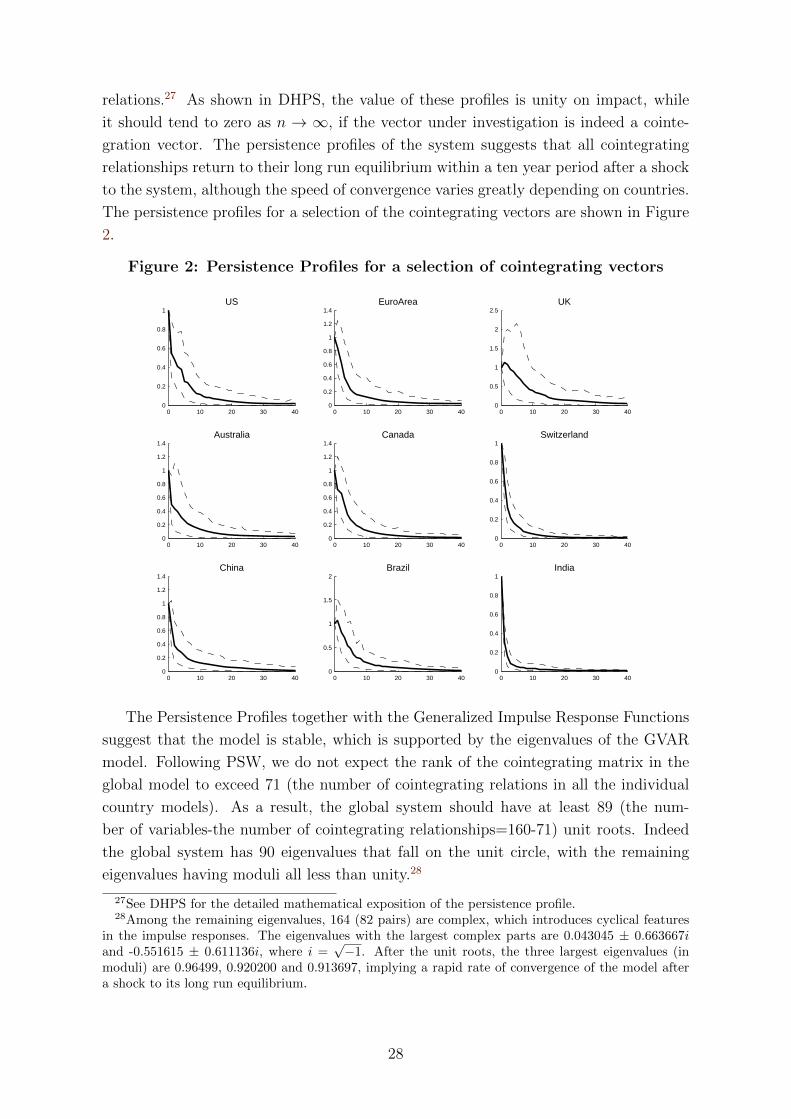
relations.27 As shown in DHPS, the value of these profiles is unity on impact, while

it should tend to zero as n → ∞, if the vector under investigation is indeed a cointe-

gration vector. The persistence profiles of the system suggests that all cointegrating

relationships return to their long run equilibrium within a ten year period after a shock

to the system, although the speed of convergence varies greatly depending on countries.

The persistence profiles for a selection of the cointegrating vectors are shown in Figure

2.

Figure 2: Persistence Profiles for a selection of cointegrating vectors

0 10 20 30 400

0.2

0.4

0.6

0.8

1US

0 10 20 30 400

0.2

0.4

0.6

0.8

1

1.2

1.4EuroArea

0 10 20 30 400

0.5

1

1.5

2

2.5UK

0 10 20 30 400

0.2

0.4

0.6

0.8

1

1.2

1.4Australia

0 10 20 30 400

0.2

0.4

0.6

0.8

1

1.2

1.4Canada

0 10 20 30 400

0.2

0.4

0.6

0.8

1Switzerland

0 10 20 30 400

0.2

0.4

0.6

0.8

1

1.2

1.4China

0 10 20 30 400

0.5

1

1.5

2Brazil

0 10 20 30 400

0.2

0.4

0.6

0.8

1India

The Persistence Profiles together with the Generalized Impulse Response Functions

suggest that the model is stable, which is supported by the eigenvalues of the GVAR

model. Following PSW, we do not expect the rank of the cointegrating matrix in the

global model to exceed 71 (the number of cointegrating relations in all the individual

country models). As a result, the global system should have at least 89 (the num-

ber of variables-the number of cointegrating relationships=160-71) unit roots. Indeed

the global system has 90 eigenvalues that fall on the unit circle, with the remaining

eigenvalues having moduli all less than unity.28

27See DHPS for the detailed mathematical exposition of the persistence profile.28Among the remaining eigenvalues, 164 (82 pairs) are complex, which introduces cyclical features

in the impulse responses. The eigenvalues with the largest complex parts are 0.043045 ± 0.663667iand -0.551615 ± 0.611136i, where i =

√−1. After the unit roots, the three largest eigenvalues (in

moduli) are 0.96499, 0.920200 and 0.913697, implying a rapid rate of convergence of the model aftera shock to its long run equilibrium.

28

6.2 Contemporaneous effects of foreign credit on domestic

credit

To examine the international linkages between domestic credit and foreign credit, in

particular the impact of foreign credit on domestic credit, we investigate the contempo-

raneous effects of foreign variable on their domestic counterparts, with robust t ratios

computed using White’s heteroskedasticity-consistent variance estimator. These esti-

mates can be interpreted as impact elasticities of domestic to foreign variables.

Consistent with the findings for the cross-country correlation in the earlier sec-

tion, we observe positive and significant elasticities in foreign and domestic credit in

a large number of industrialized countries, but only one emerging market economy

(Brazil), which indicates that credit in countries with mature banking sector are more

inter-related with the rest of the world. Specifically, for the UK, the euro area and

Switzerland, a 1% change in foreign credit in a given quarter leads to an increase in

domestic real credit of 0.48%, 0.23% and 0.38% respectively, within the same quarter.

The contemporaneous effect of foreign credit on real credit in China and India is pos-

itive but not significant, despite the rapid development of banking sector in the two

largest emerging economies, reflecting a much lower degree of openness in the banking

sector in comparison to more advanced economies.

Table 13: Contemporaneous effects of foreign variables on their domesticcounterparts

Country Domestic variables

yt ∆pt qt ρSt ρLt crdt

US 0.712 0.213 - 0.036 - -[5.141] [2.443] - [0.806] - -

Euro Area 0.517 0.057 1.009 0.068 0.67 0.225[5.138] [1.395] [18.371] [3.938] [8.134] [2.143]

UK 0.261 0.371 0.88 0.163 0.757 0.48[1.634] [1.988] [16.435] [1.379] [5.305] [2.95]

Japan 0.384 0.061 0.635 -0.047 0.549 -0.085[2.279] [0.457] [5.064] [-1.105] [6.532] [-0.622]

Sweden 1.33 0.572 1.174 0.348 0.891 1.989[4.822] [2.724] [13.39] [2.237] [7.328] [4.123]

Switzerland 0.622 0.219 0.924 0.163 0.386 0.377[4.716] [1.667] [12.226] [2.616] [5.05] [2.492]

China 0.022 0.285 - 0.054 - 0.06[0.195] [0.827] - [1.604] - [0.157]

Brazil 0.649 0.62 - 1.045 - 2.605[1.737] [0.501] - [0.526] - [3.138]

India -0.226 0.506 0.757 0.009 - 0.464[-0.861] [1.479] [4.22] [0.24] - [0.85]

Singapore 1.162 0.464 1.27 0.377 - -0.01[5.609] [3.031] [11.811] [1.942] - [-0.061]

Note: White heteroskedastic-robust t-ratios are given in square brackets.

29

In addition, results suggest high elasticity of foreign and domestic long run interest

rates (statistically significant), implying relatively strong co-movements between the

international bond markets. Contemporaneous financial linkages in the equity market

are found to be strong and significant, in particular, we observe above unit elasticity in

the euro area, Sweden and Singapore, which indicates a high degree of synchronization

in the international equity markets.

6.3 Generalized impulse response functions

To study the dynamic properties of the global model and to assess the time profile of the

effects of variable-specific shocks, we investigate the implication of (1) a one standard

error negative shock to US real credit, (2) a one standard error negative shock to US

real equity prices and (3) a one standard error positive shock to oil prices, using the

Generalized Impulse Response Function (GIRF) (see Koop, Pesaran, and Potter, 1996

and Pesaran and Shin, 1996). In contrast to the Orthogonalized Impulse Responses

(OIR) proposed by Sims (1980), GIRF is invariant to the ordering of the variables and

the countries in the GVAR model, which offers more flexibility in the modeling strategy

without making any a priori assumption on the sequence of impacts. GIRF is particular

applicable to our global framework, which contains 160 real and financial variables

covering 26 advanced and emerging economies in the world. It would be very difficult

to impose a sensible ordering among the 160 variables based on existing economic

theory, especially given that the mechanism through which shocks are transmitted is

likely to have evolved during the long sample period from 1979 to 2006. Note that

GIRF and OIR coincide if the error variance matrix is diagonal, in the case of a non-

diagonal error variance matrix, the two impulse responses are the same only for shocks

to the first equation in the VAR (see Pesaran and Shin, 1996 for a formal proof).

In the interpretation of the GIRF results, we focus only on the first two years

following the shock since we are interested in studying their impact on the international

short-term business cycles fluctuations and the two year time horizon seems to be a

reasonable time horizon for this purpose.

6.3.1 Shock to US real credit

Consider first the GIRFs for a one standard error negative shock to US real credit,

which is equivalent to a fall of around 0.9-1% per quarter. The real credit shock results

in a permanent fall in US real credit of around 2% at two year horizon, reflecting the

persistence of the credit series. The impulse response function suggests strong evidence

of international spillover of credit shocks, which is consistent with our earlier finding

of a significant contemporaneous impact of foreign credit on domestic credit, especially

for advanced economies.

The GIRFs show that the transmission of the real credit shock to the euro area,

UK and Japan real credit takes place rather quickly, with the impact on UK real credit

30

Figure 3: GIRFs of a one standard deviation negative shock to US realcredit (bootstrap mean estimates with 90% error bounds)

0 5 10 15 20−0.035

−0.03

−0.025

−0.02

−0.015

−0.01

−0.005

0US Real Credit

0 5 10 15 20−0.05

−0.04

−0.03

−0.02

−0.01

0

0.01UK Real Credit

0 5 10 15 20−0.05

−0.04

−0.03

−0.02

−0.01

0

0.01Japan Real Credit

0 5 10 15 20−0.025

−0.02

−0.015

−0.01

−0.005

0

0.005Euro Area Real Credit

0 5 10 15 20−0.04

−0.03

−0.02

−0.01

0

0.01Switzerland Real Credit

0 5 10 15 20−0.08

−0.06

−0.04

−0.02

0

0.02Sweden Real Credit

0 5 10 15 20−0.03

−0.02

−0.01

0

0.01

0.02China Real Credit

0 5 10 15 20−0.025

−0.02

−0.015

−0.01

−0.005

0

0.005

0.01Singapore Real Credit

0 5 10 15 20−0.1

−0.05

0

0.05

0.1Brazil Real Credit

especially strong at around 1.5% after one year, possibly due to the strong linkages in

the banking sector between the US and the UK. We also observe the spillover of credit

shock to emerging market economies, such as Singapore and Brazil, where the negative

impact on the real credit variable is significant in the first three or four quarters,

however the negative impact on China real credit is not statistically significant. One

possible explanation is the greater openness of the banking sector and capital markets

in Singapore and Brazil in comparison to China. A greater presence of global banks

in Singapore and Brazil also makes their domestic banking sector more susceptible to

credit shocks originated in the US.

The real credit shock is transmitted to the real economy, as seen by a decline in US

real GDP of around 0.15% on impact, by 0.5% at the end of two quarters, although the

process starts to reverse after one year. The impact on the euro area, UK and Japan

real GDP is negative and significant, at around 0.2% to 0.3% on average (see Figure 4).

As predicted by economic theory, a decline in credit (either through a fall in demand

or a shortage in credit availability) is accompanied by a fall in firm investments and a

reduction in output in the economy. The subsequent spillover in the real economy could

be a result of the strong trade linkages between US, the euro area, UK and Japan.

The negative shock to US real credit is accompanied by decreases in short term

interest rates in the US, UK, the euro area and several other advanced economies,

suggesting a possible loosening of monetary policy in association with the fall in the

availability of credit, as observed in the policy coordination in the aftermath of the

31

Figure 4: GIRFs of a one standard deviation negative shock to US realcredit–cont. (bootstrap mean estimates with 90% error bounds)

0 5 10 15 20−10

−8

−6

−4

−2

0

2

4x 10

−3 US Real GDP

0 5 10 15 20−8

−6

−4

−2

0

2

4x 10

−3 UK Real GDP

0 5 10 15 20−0.025

−0.02

−0.015

−0.01

−0.005

0

0.005Japan Real GDP

0 5 10 15 20−12

−10

−8

−6

−4

−2

0

2x 10

−3 Euro Area Real GDP

0 5 10 15 20−15

−10

−5

0

5x 10

−3Switzerland Real GDP

0 5 10 15 20−15

−10

−5

0

5x 10

−3 Sweden Real GDP

0 5 10 15 20−3

−2.5

−2

−1.5

−1

−0.5

0

0.5x 10

−3 US Short Term IR

0 5 10 15 20−4

−3

−2

−1

0

1x 10

−3 UK Short Term IR

0 5 10 15 20−2.5

−2

−1.5

−1

−0.5

0

0.5x 10

−3 EA Short Term IR

0 5 10 15 20−0.04

−0.03

−0.02

−0.01

0

0.01

0.02

0.03US Real Equity Price

0 5 10 15 20−0.1

−0.08

−0.06

−0.04

−0.02

0

0.02UK Real Equity Price

0 5 10 15 20−0.2

−0.15

−0.1

−0.05

0

0.05Euro Area Real Equity Price

recent credit crunch. The impact of the real credit shock is also reflected in a significant

fall in the UK and European equity markets at around 3 to 4%, possibility reflecting

a fall in investor confidence and a deterioration in the economic fundamentals in the

economy.

6.3.2 Shock to US equity prices

The GIRFs of a one standard error negative shock to US equity prices are given in

Figure 5. This shock amounts to around 5% fall in US real equity prices per quarter.

The negative equity shock has a permanent impact on US real equity price at 5% on

average in a two year horizon.

The spillover to the UK, the euro area and Japan equity market takes place rather

quickly and the effects of the shock are statistically significant. On impact, equity

prices in these markets fall by a similar amount to the US market at around 5%, but

32

the effect of the US shock on the European and Japanese equity markets becomes more

pronounced over the first two years. This result is consistent with findings in DdPS

(based on an earlier data set ending in 2003Q4) and suggests a mild overreaction of

equity prices in the European markets to the US shock, reflecting the higher volatility

of the European equity markets compared with that of the US market (where S&P500

is used as the equity benchmark). The spillover in the equity market is not limited

to advanced economies, we also observe a significant and negative impact of US eq-

uity shock on the real equity prices of emerging market economies such as India and

Singapore, again consistent with our findings in the contemporaneous effect of foreign

variables on their domestic counterparts, where the elasticity of a foreign equity shock

is found to be significant for both advanced and emerging market economies.

The equity price shock is accompanied by a decline in US real GDP of around 0.15%

on impact and about 0.6% in two year horizon. The impact on UK real GDP is similar

to that of the US credit shock in the first year, at around 0.2%, but the effect is no

longer significant after the first year. Real output in the euro area falls by around 0.4%

to 0.6% before reverting back to zero after the first year.

Similar to a US real credit shock, a negative shock to US real equity prices is

associated with a fall in short term interest rates in the US, UK and the euro area,

possibly reflecting a loosening in monetary policy stance. In contrast to the case of

a US real credit shock, a negative shock to US real equity prices is also accompanied

by a significant fall in long term interest rates in advanced economies including the

US, UK and Japan, suggesting that equity markets can be more effective in conveying

information on the fundamentals and growth prospect of the economy and in reflecting

private sector’s expectation on central banks’ monetary policy decisions.

6.3.3 Shock to oil prices

We are interested in studying the shocks to oil prices since oil price changes have had

a significant impact on output growth, inflation and the conduct of monetary policy

in the past thirty years. A positive unit shock to oil prices results in a 10% increase

per quarter in oil prices. This shock is accompanied by a negative and statistically

significant decline of real output in China and the UK (however, the impact on US real

output was not statistically significant). In particular the fall in real output in China

is as high as 1% in two year horizon, reflecting the high dependence of the Chinese

economy on oil imports.

On impact, the oil price shock raises the inflation rate in US and the euro area by

0.2% and 0.1% respectively, before it starts to fall to about half of the initial increase

in two year horizon (see Figure 6). Similar to the findings in DdPS, the GIRFs suggest

the effects are stronger on US inflation compared to euro area inflation.

As expected, the increase in oil prices is associated with a fall in major equity

markets. The impact on European equity markets are stronger as compared with the

US and UK equity markets, at around 5% in two year horizon, again a result of a higher

33

Figure 5: GIRFs of a one standard deviation negative shock to US realequity price (bootstrap mean estimates with 90% error bounds)

0 5 10 15 20−0.1

−0.08

−0.06

−0.04

−0.02

0US Real Equity Price

0 5 10 15 20−0.12

−0.1

−0.08

−0.06

−0.04

−0.02

0

0.02UK Real Equity Price

0 5 10 15 20−0.25

−0.2

−0.15

−0.1

−0.05

0Euro Area Real Equity Price

0 5 10 15 20−0.2

−0.15

−0.1

−0.05

0Japan Real Equity Price

0 5 10 15 20−0.35

−0.3

−0.25

−0.2

−0.15

−0.1

−0.05

0India Real Equity Price

0 5 10 15 20−0.4

−0.3

−0.2

−0.1

0Singapore Real Equity Price

0 5 10 15 20−15

−10

−5

0

5x 10

−3 US Real GDP

0 5 10 15 20−5

0

5

10x 10

−3 UK Real GDP

0 5 10 15 20−0.01

−0.005

0

0.005

0.01Euro Area Real GDP

0 5 10 15 20−4

−3

−2

−1

0

1x 10

−3 US Short Term IR

0 5 10 15 20−4

−3

−2

−1

0

1

2x 10

−3 UK Short Term IR

0 5 10 15 20−2

−1.5

−1

−0.5

0

0.5

1x 10

−3 EA Short Term IR

0 5 10 15 20−2.5

−2

−1.5

−1

−0.5

0

0.5

1x 10

−3 US Long Term IR

0 5 10 15 20−1.5

−1

−0.5

0

0.5

1x 10

−3 UK Long Term IR

0 5 10 15 20−15

−10

−5

0

5x 10

−4 Japan Long Term IR

volatility of the European benchmark equity prices compared with that of the US and

UK.

6.4 Robustness of the GVAR results to time-varying weights

Recall that the analysis was based on three year average trade weights between 2001

and 2003, to check the robustness of our results to the choice of trade weight, we also

estimate the GVAR model using the time-varying weights, constructed as rolling three

year moving averages of the annual trade weights. First, we study the relationship of

34

Figure 6: GIRFs of a one standard deviation positive shock to Oil Prices(bootstrap mean estimates with 90% error bounds)

0 5 10 15 20−0.025

−0.02

−0.015

−0.01

−0.005

0

0.005China Real GDP

0 5 10 15 20−8

−6

−4

−2

0

2

4x 10

−3 UK Real GDP

0 5 10 15 20−8

−6

−4

−2

0

2x 10

−3 US Real GDP

0 5 10 15 20−0.05

−0.04

−0.03

−0.02

−0.01

0

0.01US Real Equity Price

0 5 10 15 20−0.08

−0.06

−0.04

−0.02

0

0.02UK Real Equity Price

0 5 10 15 20−0.15

−0.1

−0.05

0

0.05Euro Area Real Equity Price

0 5 10 15 20−1

0

1

2

3x 10

−3 US Inflation

0 5 10 15 20−5

0

5

10

15x 10

−4 Euro Area Inflation

0 5 10 15 200

0.05

0.1

0.15

0.2US POIL

the two measures, x∗it (based on fixed weights) and x∗∗it (based on time-varying weights).

The correlation coefficients between the levels and first differences of the two measures

are given in Table 14. Similarly to DdPS, we find that the correlation coefficients of the

levels of the variables being very close to unity, while the correlations in terms of first

differences are not as high, particularly in the case of inflation rates and credit. Given

the high correlations in the levels of the series, we conjecture that the main conclusions

of the paper is unlikely to be affected by whether fixed or time-varying trade weights

are used. We find that this is indeed the case.

By re-estimating the GVAR model using time-varying weights, we find that the

same number of lag orders pi and qi are chosen for the individual VARX∗(pi, qi) model

and we obtain similar number of cointegration relationships. Compared with Table

4, we estimate a time-varying GVAR model with the same number of cointegration

relationships for all countries, except for Argentina, Brazil, Indonesia, Turkey, where

the number of cointegrating relationships was decreased by one, and for Chile, Malaysia,

Philippines, Singapore, India, Saudi Arabia and Switzerland, where the number of

cointegrating relations was increased by one.29

With regard to the impact effects of the foreign variables, we obtain similar results,

especially in the case of real output, real equity prices, short term and long term

interest rates. The results from the Generalized Impulse Response Functions (GIRF)

for a one standard error negative shock to US real credit, equity and a one standard

29For Mexico, the number of cointegrating relationships decreases by two.

35

Table 14: Correlation coefficients of country-specific foreign variables usingfixed and time-varying trade weights

Country Real output Inflation Real equity pricesLevels 1st diff. Levels 1st diff. Levels 1st diff.

US 1.00 0.88 0.90 0.71 1.00 0.99UK 1.00 0.98 0.95 0.68 1.00 1.00

China 1.00 0.285 0.45 0.01 0.99 0.98Euro Area 1.00 0.88 0.88 0.49 1.00 1.00

Japan 1.00 0.83 0.79 0.43 1.00 0.99Sweden 1.00 0.98 0.89 0.50 1.00 1.00

Switzerland 1.00 0.99 0.90 0.51 1.00 1.00

Country Short term interest rates Long term interest ratesLevels 1st diff. Levels 1st diff.

US 0.98 0.96 1.00 0.99 – –UK 1.00 0.99 1.00 1.00 – –

China 0.97 0.94 0.99 0.94 – –Euro Area 0.99 0.99 1.00 1.00 – –

Japan 0.99 0.98 1.00 0.99 –Sweden 1.00 0.99 1.00 1.00 – –

Switzerland 1.00 0.97 1.00 1.00 – –

Country Real exchange rates Real creditLevels 1st diff. Levels 1st diff. – –

US 0.98 0.85 0.89 0.23 – –UK 1.00 0.98 1.00 0.52 – –

China 0.84 0.62 0.92 0.12 – –Euro Area 0.97 0.88 0.98 0.36 – –

Japan 0.77 0.53 0.99 0.35 – –Sweden 1.00 0.99 0.98 0.45 – –

Switzerland 1.00 0.99 1.00 0.81 – –

error positive shock to oil prices are also found to be similar, except for a few cases

on the significance of the responses. For example, a negative shock to US credit now

has significant (negative) impact on US and Japan equity when re-estimating with

time-varying weights.

7 Conclusion

This paper investigates the important role of bank credit in the international business

cycles using a Global VAR framework containing 26 economies, estimated over the

period 1979Q2 to 2006Q4. We find robust results from the country specific VARX∗

models that the incorporation of credit provides statistically significant improvement in

explaining output growth, changes in inflation and long run interest rates for countries

with developed banking sector. Our results confirm the theoretical predictions that

credit market conditions could lead to direct impact on the real economy and highlight

the importance of the credit variable in explaining the dynamics of business cycle

fluctuations and the value of incorporating credit in economic modeling.

36

The impulse responses of a negative shock to US credit shed light on interesting

insights of the international transmission of credit shocks. First, we find strong evidence

of international spillover of US credit shocks to the euro area, UK and Japan, with the

impact on the UK particularly profound, possibly due to the strong linkages in the

banking sectors between the UK and the US. Second, the model predicts the spillover

of credit shock to the US real economy and its subsequent international propagation in

the real sector. Indeed, the interactions between financial market and the real economy

is not simply a one way process. A shock to US credit is accompanied by falling output

in the US, UK and the euro area for 12 to 18 months, as shown in our analysis. Third,

the US credit shock is associated with a fall in short term interest rates in several

economies including the US, UK and the euro area, suggesting a possible loosening

of monetary policy in response to the contraction in credit availability, as observed

in the policy coordination in the aftermath of the recent credit crunch. Furthermore,

US credit shock is accompanied by a significant fall in the UK and European equity

markets. Our results are consistent with the theoretical insights that credit markets

play an important role in the international transmission of shocks, resulting a magnified

impact of the initial shock and highly correlated business cycles across countries during

the downturn.

In addition to the US credit shock, we examine the impact of a one standard error

negative shock to US real equity price and a one standard error positive shock to oil

prices. A negative shock to US real equity is transmitted rather quickly to equity

markets in advanced as well as emerging economies, with the impact on the European

and Japanese markets particularly profound. The US equity shock is also accompanied

by a fall in real output, short term and long term interest rates in several advanced

economies, such as the US, UK and Japan. For a positive shock to oil prices, we observe

a significant fall in real output in China, reflecting the high dependence of the Chinese

economy on oil imports, and a rise in inflation in US and the euro area.

The generalized impulse response functions of a negative shock to US real credit,

US real equity prices and a positive shock to oil prices provide strong evidence of the

international spillover of financial shocks and shed light on the mechanisms through

which financial shocks are transmitted across country borders. In particular, the rapid

international transmission of credit shocks and the profound impact on the international

financial markets and the global real economy highlights the important role of credit

in international business cycles and calls for greater attention to credit measures in

economic policy making.

37

A Data Appendix

A1 Data sources

The credit variable in our analysis measures bank credit to the private sector. Ourmain sources for the credit data are the IMF International Finance Statistics (IFS)and Datastream.30 The Datastream credit data are drawn from National Sources andthe OECD Main Economics Indicators. For the rest of the variables considered in theGVAR, the data source is drawn from Dees, Pesaran, Smith, and Smith (2009) and therejoinder of Pesaran, Schuermann, and Smith (2009).

In terms of country coverage and time coverage, the IFS statistics is more completefor the 33 countries considered in the GVAR from 1979Q1 to 2006Q4 (among which8 countries are later grouped together as the Eurozone), compared with Datastream.To draw meaningful comparison between the 33 countries, maintain the consistency ofthe definition of the credit series and reduce errors due to assessing data from differentstatistical sources, we have decided to use the IMF IFS database as our primary sourcefor the credit data and Datastream as a secondary source.31

The source of credit data for all 33 countries, except UK, Australia and Canada,was the series ‘Claims on Private Sector from Deposit Money Banks’ (22d) from theIFS Money and Banking Statistics, measured in national currency in current prices.The data source for the UK and Australia was the National Statistics from Datastreamand for Canada was the OECD data from Datastream

A1.1 Choice of the credit variable (IFS series)

The choice of the appropriate credit variable is guided by existing literature, dataavailability and the consideration of international comparability between country series.

There are a few important decisions to be made with regard to our chosen measureof bank credit to the private sector. First, the definition of the banking sector. Wechoose to follow the definition of ‘deposit money banks’ in the IFS Money and BankingStatistics. Deposit money banks comprise commercial banks and other financial insti-tutions that accept transferable deposits, such as demand deposits. They often engagein core banking services that extend loans to the non-financial corporations, which ul-timately determine the level of investment and output in the economy, as shown in thetheoretical literature on credit.

In addition to ‘deposit money banks’, IFS also publish data on ‘other bankinginstitutions’, which comprise institutions that do not accept transferable deposits butthat perform financial intermediation by accepting other types of deposits or by issuingsecurities.32 We have decided not to include ‘other banking institutions’ in our definition

30Several studies in the finance and development literature, see for example Baltagi, Demetriades,and Law (2008), used the World Development Indicators (WDI) (published by the World Bank) as thesource for credit data (private credit as a percentage of GDP). The credit data in WDI is also takenfrom the IMF International Finance Statistics, for example, the indicator “Claims on private sector”in WDI is taken from IFS line 32d, which includes gross credit from the financial system (monetaryauthority and deposit money banks) to the private sector.

31Further, the OECD data on credit to the private sector was discontinued at the beginning of 2007.For the purpose of updating the database in the future, we have decided not to use the OECD creditseries unless necessary.

32For example, other banking institutions covers savings and mortgage loan institutions, post-officesaving institutions, building and loan associations, finance companies that accept deposits or deposit

38

of banking sector for two reasons. First, ‘other banking institutions’ often focus onconsumer mortgages loans business and security investment, rather than core lendingservices to the private sector that is of interest to our analysis. For example, in theUS, mortgages make up close to 70 percent of the credit market instruments held bysavings institutions (part of ‘other banking institutions’).33 Further, the data on ‘otherbanking institutions’ is missing for 15 out of 33 countries considered in the GVAR.34

Where available, the measure ‘claims on private sector from other banking institutions’(42d) does not have complete time coverage for the period 1979Q1 to 2006Q4.

We also note that our interests lie in the role of the commercial banking sector ratherthan the central bank in the provision of credit, as a result, we do not include monetaryauthority in our definition of the banking sector and the measure of ‘claims on privatesector in the monetary survey’ (32d) is not appropriate in our study (where monetarysurvey consolidates the account of the Central Bank and deposit money banks).

Second, our credit measure (claims on private sector from deposit money banks)isolates credit issued to the private sector, as opposed to credit issued to governments,government agencies, and public enterprises, following the empirical literature on fi-nance and development. In the development literature, credit to the private sector (asexpressed as percentages of GDP) is considered the most important banking develop-ment indicator, since it proxies the extent to which new firms have opportunities toobtain bank finance and it closely accords to the McKinnon-Shaw school’s inside moneymodel which asserts that it is the supply of credit to the private sector that determinesboth the level and component of investment. This in turn could influence the level ofoutput and economic growth and better economic prospects could lead to increasedflow of bank credit to the private sector, see for example Masih (2001).

One potential limitation of the measure ‘claims on the private sector from depositmoney banks’ is that the private sector is composed of both individuals and non-financial corporations in the IFS statistics (no separate series are available), while ourpreferred credit measure is bank lending to non-financial corporations. Although somenational sources publish separate series for bank credit to individuals and non-financialcorporations (see for example the Fed Flow of Funds accounts), this measure can not befound in all the 33 countries considered in the GVAR (for example, the Bank of Japanalso groups bank credit to individual and non-finance corporations in their money andbanking data). In order to maintain the consistency of the definition of ‘private sector’in our analysis, we have decided to follow the IFS definition and use the series ‘claimson the private sector from deposit money banks’ (22d) as our preferred measure forprivate credit.

In addition, we explored the possibility of using a broader credit measure ‘domesticcredit’ (line 32), which is the sum of the claims on central government, state and localgovernment, non-financial public entreprises, private sector, other bank institutions andnon bank financial institutions in the monetary survey. The measure ‘domestic credit’captures the net credit available in the economy, with its components measuring thenet rather than gross claims on the different sectors, such as net claims on centralgovernment. Since we are interested in the level of credit used for investment and

substitutes, development banks and offshore banking institutions.33See ‘Guide to the Flow of Funds account’ published by the Federal Reserve Statistical Release at

http://www.federalreserve.gov/releases/z1/current/ for more details.34 The data category ‘other banking institutions’ is not available for the following countries: Aus-

tralia, Austria, Belgium, China, Finland, France, Germany, India, Indonesia, Italy, Japan, Spain,Thailand, Turkey and United Kingdom.

39

production, rather than the transfer of credit between different sectors in the economy,‘domestic credit’ is not an appropriate measure for our purpose. Furthermore, the othercomponents ‘claims on non-financial public enterprises’ and ‘claims on other bankinginstitutions’ of ‘domestic credit’ are often very small compared with ‘claims on theprivate sector’.35

Third, we choose to use the level of ‘claims on private sector from deposit moneybanks’ rather than its ratio to GDP, as seen in the finance and development literature.36

The reason is that our objective is not to study the extent of financial intermediation inthe economy but the overall level of bank credit that is available to the private sector.

Our preferred Datastream series has a definition that is closest to the IFS series anda similar magnitude. Several studies on the role of credit also adopt the same creditmeasure, see for example Goodhart and Hofmann (2008) and Levine and Zervos (1998).

A1.2 Data on the Euro Zone

For countries within the Eurozone, two series are available for the measure ‘Claimson Private Sector from Deposit Money Banks’. One series is denominated in nationalcurrency for the period from 1979Q1 to 1998Q4 (series 22d.zf), before the introductionof the Euro, the other series is denominated in euros from 1999Q1, after the introduc-tion of the euro (series 22d.zw). The latter series is compiled on the base of nationalresidency criteria (as oppose to Euro Area-wide residency criteria), described in thefifth edition of the IMF Balance of Payment Manual.

The former series denoted in national currency is converted into euro using an ap-propriate exchange rate series between euro and national currency. This exchange rateseries is constructed using the ratio of two series, one being the synthetic Eurodollarexchange rate from Datastream, the other the exchange rate of dollar to national cur-rency (consistent with the exchange rate used to derive the euro dollar rate in DdPS).37

In DdPS, quarterly averages of daily Datastream GTIS US$ exchange rate data, cal-culated based on the last Wednesday of each month within the quarter, are used forBrazil (1994Q1-2006Q4), Chile (1994Q1-2006Q4), Peru (1991Q1-2006Q4). For the restof the countries (1986Q1-2006Q4), the rate of change of the IFS series ‘rf.zf’ is used tobackfill the series to 1979Q1.

35The measure ‘domestic credit’ can sometimes be negative (due to negative net claims on centralgovernment), while in fact bank credit to the private sector was in steady growth in the economy forthe corresponding period, see for example Saudi Arabia from 1979Q1 to 1987Q3.

36For example, King and Levine (1993a,b) use the ratio of gross claims on the private sector (line32d) to GDP in their study. Levine and Zervos (1998) and Levine (1998) use the ratio of deposit moneybank credit to the private sector (line 22d) to GDP over the period 1976 to 1993. Levine, Loayza,and Beck (2000) uses a measure of private credit as an indicator of financial intermediary developmentfrom 1960 to 1995, where Private credit equals the ratio of credits by financial intermediaries to theprivate sector (line 22d+42d) to GDP.

37The synthetic Euro/US exchange rate in Datastream is constructed as follows: The EMU (Eu-ropean Monetary Unit) in national currencies are weighted by 1996 national GDP levels, and thenexpressed in Deutschmark terms using the bilateral rates set by the EU (implicitly taken as the bestapproximation to the fixed bilateral rates that will prevail on December 31, 1998). The individualcomponents are each converted to Deutschmarks at current exchange rates using the Reuters ClosingSpot Rates. Finally, by multiplying the series by the fixed Deutschmark/Euro rate, Datastream pro-duces a Deutschemark/Euro exchange rate that reflects both the changing relative strengths of theEMU in countries over time and the presumed fixed local to Euro bilateral rates. By converting theseries using the appropriate US/Deutschmark rate, also taken from Reuters, a synthetic Euro/US rateis constructed. Documentation is available on-line at www.datastream.com.

40

A1.3 Datastream credit series

As mentioned earlier, the series on credit to private sector in Datastream are takenfrom National Sources and the OECD Main Economics Indicators.38 The credit seriesfor Australia, Canada and the UK are taken from Datastream. A brief description ofthe series are given below.

For Australia, we use the datastream series (AUBANKLPA) from the Reserve Bankof Australia, which captures loans and advanced by banks, which includes all bank loansand advances to the private sector (including public trading enterprises) on the balancesheet of banks, net of loans to non-bank financial institutions (NBFIs).

For Canada, we use an OECD series (CNOCR016A) “credit to the private sector”,which consists of consumer credits, residential mortgage credits, short-term (businessloans, chartered bank foreign currency loans, banks’ acceptances, commercial paperissued by non-financial corporations) and other (non-residential mortgages, leasing re-ceivables, bonds and debentures, equity and other) business credit.

Finally, for the UK, we take a credit series from the Bank of England that measuresbank and building society lending (UKVQJMQ.). This series represents the seasonallyadjusted quarterly amounts outstanding of M4 lending (monetary financial institutions’sterling net lending to private sector) made by Banks and Building societies; where theM4 private sector consists of all UK residents other than the public sector and MFIs.39

The description of the Datastream series on credit for other countries is not pre-sented here due to space considerations, but available upon request.

A1.4 Comparison between IFS and Datastream credit data

The choice of the appropriate credit series between the IFS and the Datastream series ona country by country basis is guided by two principles. First of all, we use the IFS serieswhen no alternative series is available from Datastream or the available Datastreamseries have missing observations for more than a year. Second, for countries with fullseries available in Datastream, we compare the logarithms of the credit data in levelsand first differences between IFS and Datastream and choose the series that are moreconsistent with the credit history of the country.40 For Australia, Canada and UK, theDatastream series significantly improve upon the IFS credit series, where the spike inthe Australia series in 1985 and the movement in the Canada and UK series at thebeginning of the 80s can not be explained by the credit history in these economies.The spikes could be a result of measurement errors or a change in the definition ofbanking sector (although the level shift due to a change in definition have already beenaccounted for). We have decided to replace the IFS series with the Datastream seriesfor Australia, Canada and the UK. For the rest of the countries, the Datastream seriesdo not provide an improvement upon the IFS series and we decide the keep the creditseries from the IFS database. In particular, the IFS series for the US reflects a moreprofound credit cycle, which is consistent with the credit history in the US and the

38In datastream, the relevant credit series are available for the 33 countries in the GVAR exceptfor Argentina and Saudi Arabia, however, only a number of countries have series for the full periodfrom 1979Q1 to 2006Q4, namely Australia, Canada, France (data is missing from 1979Q1 to 1979Q4),Germany, Japan, Korea, Norway, South Africa, Spain, Turkey, the United Kingdom and the UnitedStates. Note also, the OECD credit series were discontinued from 2007Q2.

39 For details, see http://www.bankofengland.co.uk/mfsd/iadb/notesiadb/M4 counterparts.htm40The countries include Australia, Canada, France, Germany, Japan, Korea, Norway, South Africa,

Turkey, the United Kingdom and the United States.

41

changes in commercial credit standards as shown in the Loan Officer Opinion Survey,see for example Lown and Morgan (2006) and Lown, Morgan, and Rohatgi (2000).41

A2 Adjustments to credit data

A2.1 Interpolation

The countries with complete data series for ‘Claims on private sector from DepositMoney Banks’(22d) are Argentina, Australia, Canada, Chile, India, Japan, Korea,Malaysia, Mexico, New Zealand, Peru, Singapore, Switzerland, Thailand, Turkey, UKand US. Some observations are missing for the following countries (missing data inbracket): 1) EU countries: Austria (1998Q4), Belgium (1998Q4), France (1998Q3 to1998Q4), Netherlands (1998Q1 to 1998Q4). 2) Ex-EU countries: Brazil (1986Q3 to1988Q1), China (1979Q1 to 1985Q3), Indonesia (1979Q1 to 1979Q4), Norway (1987Q1and 1987Q2), Philippines (1983Q3, 1984Q1 to 1984Q3, 1985Q1 to 1985Q3, 1986Q1to 1986Q3), Saudi Arabia (1983Q1 to 1983Q3), South Africa (1991Q3 and 1991Q4),Sweden (2001Q1 to 2001Q3).

For country series with missing observations, we interpolate the series with missingobservations using the growth rate of a comparable series when available. For China,the credit data (Claims on private sector from Deposit Money Banks, 22d) from 1979Q1to 1985Q3 is constructed by using the growth rate of the series ‘Claims on private sec-tor from Deposit Money Banks AND Monetary authority’ (32d) (the two series havesimilar growth rate for overlapping periods). For Austria, missing observations for1998Q4 was generated using the growth rate of a series from Datastream named ‘lend-ing to private sector’ (OELNBNK.A). For France, missing observations for 1998Q3 and1998Q4 were generated based on the growth rate of a Datastream series ‘loans to res-ident private sector’ (FRBANKLPA). For the Netherlands, missing observations from1998Q1 to 1998Q4 were generated using the growth rate of a series ‘bank lending to pri-vate sector’ (NLBANKLPA) from Datastream. For South Africa, missing observationsfor 1991Q3 and 1991Q4 were generated from the growth rate of a Datastream series‘bank lending to private sector’ (SABANKLPB). For Sweden, missing observations for2001Q1 to 2001Q3 were generated from the growth rate of a comparable credit series on‘bank lending to non financial corporations’ (SDBANKLPA) on Datastream. FollowingGoodhart and Hofmann (2008), missing observations in 1987Q1 to 1987Q2 for Norwaywere generated from the growth rate of an IMF series for credit extended by non bankfinancial institutions to the private sector (IFS series 42d).

In the case when comparable series are not available, we use the median growth rateof the adjacent four quarter as a proxy of the growth rate of the missing observations.For Indonesia, the credit data from 1979Q1 to 1979Q4 is constructed by using themedian growth rate of the next four quarter. For Belgium, Brazil and Saudi Arabia,missing observations (Belgium (1998Q4), Brazil (1986Q3 to 1988Q1) and Saudi Arabia(1983Q1 to 1983Q3)) were generated from the median growth rate of the previous fourquarters. In the case of Philippines, the data was missing at multiple dates, missingobservations for 1983Q3, 1984Q1 to 1984Q3, 1985Q1 to 1985Q3, 1986Q1 to 1986Q3were generated from linear interpolation (alternative national sources and internationalsources also have observations missing for the corresponding periods).

41The comparison charts for IFS and Datastream series in levels and first differences are not presentedhere due to space considerations, but are available upon request.

42

A2.2 Adjusting for level shifts in the credit data

Many of the IMF credit series (claims on the private sector from deposit money banks)displayed large level shifts due to changes in definition and re-classifications of thebanking institutions. For example, for countries in the euro area, a new reportingsystem is adopted after the introduction of the Euro (1999Q1), which consolidates theaccount of all resident units classified as other monetary financial institutions (otherMFIs). A number of countries introduced improved classifications and sectorization ofbanking institutions, which led to changes in the definition of ‘deposit money banks’over the sample period from 1979Q1 to 2006Q4. For example, the coverage of financialinstitutions in Germany was broadened to include all cooperative banks from 1985. InSingapore, post office savings deposits was classified under ‘deposit money banks’ from1998Q4 and thereafter excluded from the category ‘other banking institutions’.42

Following Stock and Watson (2003) and Goodhart and Hofmann (2008), we adjustfor these level shifts by replacing the quarterly growth rate in the period when the shiftoccurs with the median of the growth rate of the two periods prior and after the levelshift. The level of the series is then adjusted by backdating the series based on theadjusted growth rates.

The following level shifts were adjusted for (the dates at which the IMF creditseries were butt spliced and the euro was introduced): Argentina 1990Q1, 1994Q1;Australia 1989Q1, 2002Q1; Austria 1984Q1 1995Q4, 1999Q1; Belgium 1992Q4, 1999Q1;Brazil 1986Q1, 1988Q2, 2001Q4; Canada 1981Q4 2001Q4; Chile 1997Q4; China 1993Q12002Q1; France 1999Q1; Germany 1985Q4 1990Q2 1999Q1; Indonesia 1992Q4 2001Q42004Q2; Italy 1999Q1; Japan 1997Q4 2001Q4; Malaysia 1992Q1 1996Q4 2001Q4 2002Q4;Mexico 1982Q1 1997Q1 2001Q4; Netherlands 1982Q4 1999Q1; New Zealand 1988Q3;South Africa 1992Q1 2001Q4 2002Q2; Saudi Arabia 1983Q4 1992Q4; Spain 1983Q11986Q1 1999Q1; Sweden 1983Q1 1996Q1 2001Q4; Switzerland 1982Q3 1984Q4 1996Q4;Thailand 1986Q1 2001Q4 2002Q4; United Kingdom 1981Q4 1986Q3 1992Q3 1999Q3;United States 2001Q4.

Table A1: Occurrence of banking crisis in selected countries

Country Dates Description Literature

Philippines 1984Q1 Debt crisis Intal and Llanto (1998)1997Q4 Asia Financial Crisis Chan-Lau and Chen (1998)

Thailand 1998Q1 Asia Financial Crisis Chan-Lau and Chen (1998)Indonesia 1998Q3-1999Q2 Asia Financial Crisis Chan-Lau and Chen (1998)Malaysia 1983Q3 Debt crisis Hagen and Ho (2008)

1999Q1 Asia Financial Crisis Hagen and Ho (2008)Mexico 1995Q1 Mexico Peso Crisis Hagen and Ho (2008)Argentina 1989-1990 Banking Crisis Glick and Hutchison (2001)Brazil 1990 Banking Crisis Glick and Hutchison (2001)Austria 1985Q1 Banking Crisis Hagen and Ho (2008)Finland 1991Q3 Banking Crisis Kaminsky and Reinhart (1999)New Zealand 1983Q1 Banking Crisis Hagen and Ho (2007)

42In addition, Austria adopted new sectorization of accounts in 1984Q1, Brazil in 2001Q4, Finland in1991Q1, Indonesia in 1992Q4, Japan in 1998Q2 and 2001Q4, Malaysia in 2002Q4, Mexico in 2001Q4,Philippines in 1983Q4, South Africa in 2002Q2, Thailand in 2001Q4, Turkey in 2002Q4 and the UnitedStates in 2001Q4. The table with detailed definition of banking institutions (‘deposit money banks’and ‘other banking institutions’) and changes in the definition for the 33 countries in the GVAR is notpresented here due to space considerations, but available upon request.

43

Even after all the necessary adjustment on the credit series (to account for changesin the definition of banking sector), we see clear evidence of banking and economic crisesfrom the sudden drop in credit supply. For example, Mexico’s economy enjoyed a stageof rapid credit expansion from December 1988 to November 1994, till the Peso crisis tookplace in December 1994. In addition to a sudden stop of foreign capital, domestic creditprovision in Mexico contracted in 1995.43 Countries in Southeast Asia experienceda severe credit crunch during the Asia Financial Crisis in 1997-1998, as observed inthe credit series for Philippines (1997Q4), Thailand (1998Q1) and Indonesia (1998Q3-1999Q2). Table A1 reports the date of banking crisis identified by the literature, whichcould contribute to the unusual movement that we observe in the credit series.

A2.3 Seasonal Adjustments

Seasonality is identified in the credit series in the following countries Australia, Austria,Belgium, China, Finland, France, Germany, India, Italy, Japan, Mexico, Philippines,Saudi Arabia, Spain, Switzerland, Thailand, Turkey and US, according the combinedtest for the presence of identifiable seasonality.44

To seasonally adjust the level of the log real credit series (integrated of order one),we first adjust the change in the log real credit series using the X-12 quarterly sea-sonal adjustment method in Eviews, under the additive option. Then we use the firstobservation of raw series in the level of log real credit (not seasonally adjusted) andthe seasonally adjusted series of change in log real credit to accumulate the seasonallyadjusted series in the level of log real credit.

B Unit Root Tests

The ADF tests in general support the view that the credit variables are I(1) series.45

However, the unit root hypothesis is not rejected when applied to the first differencesof the logarithm of real credit (∆crd) of 11 out of 33 countries: Belgium, Finland,Germany, Japan, Norway, Philippines, Spain, Sweden, Switzerland, Thailand and theUK. Among them, the test statistics are borderline (close to the five percent criticalvalues) for all 11 countries except Japan. When unit root tests are applied to the levelsof log real credit crd, there is no evidence with which to reject the unit root hypothesis(except the credit series of Chile and Australia, which is borderline I(1) and I(0)).

As a robustness check, we also examine the results from the weighted symmetricestimation of the ADF type regressions (introduced by Park and Fuller (1995)). Similarto the ADF tests, the lag length employed in the WS unit root tests is selected by theAkaike Information Criterion (AIC) based on the standard ADF regressions. We reportthe WS statistics for the level, first differences and second difference of all the endoge-nous variables in the GVAR model in Table B2 and Table B3. Confirming the resultsusing ADF tests, we also find that the credit variables are I(1) across countries, except

43See for example http://www.cato.org/pubs/journal/cj17n3-14.html44The results of seasonality tests are not presented here due to space considerations, but are available

upon request.45Dickey-Fuller tests attempt to account for temporally dependent and heterogeneously distributed

errors by including lagged sequences of first differences of the variables in its set of regressors (seeDickey and Fuller (1981)). The results of the Augmented Dickey-Fuller (ADF) tests are not presentedhere due to space considerations but available upon request.

44

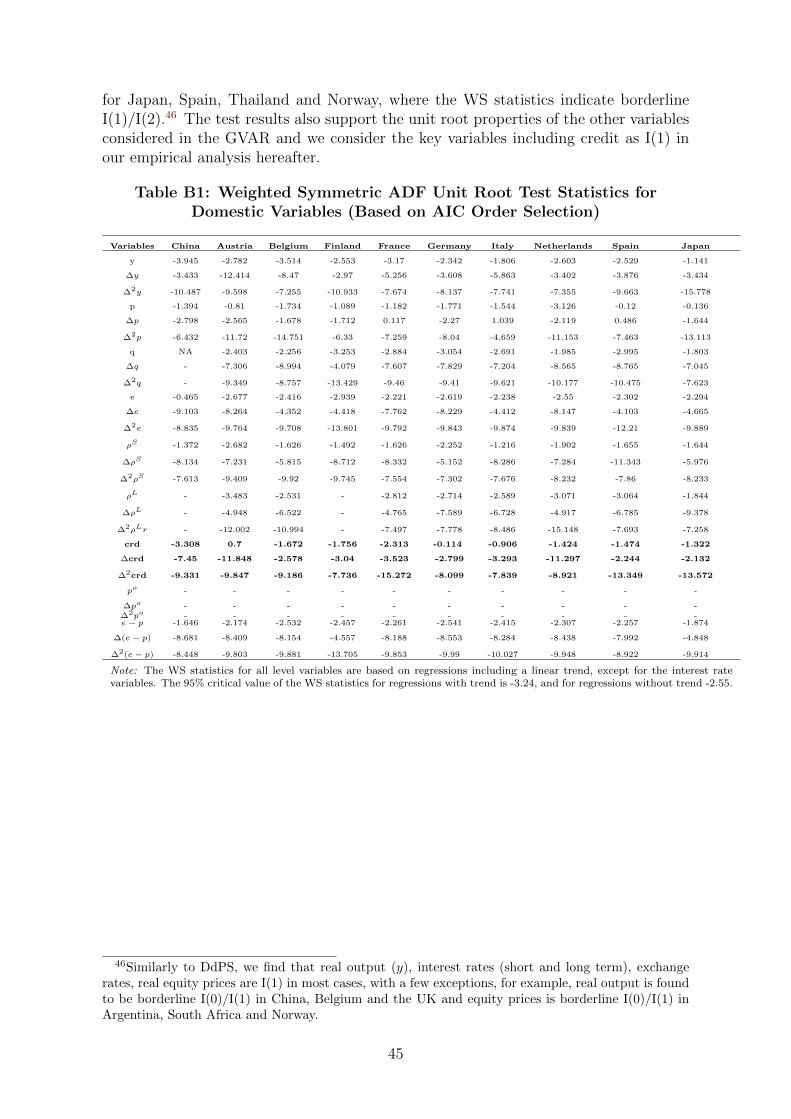
for Japan, Spain, Thailand and Norway, where the WS statistics indicate borderlineI(1)/I(2).46 The test results also support the unit root properties of the other variablesconsidered in the GVAR and we consider the key variables including credit as I(1) inour empirical analysis hereafter.

Table B1: Weighted Symmetric ADF Unit Root Test Statistics forDomestic Variables (Based on AIC Order Selection)

Variables China Austria Belgium Finland France Germany Italy Netherlands Spain Japan

y -3.945 -2.782 -3.514 -2.553 -3.17 -2.342 -1.806 -2.603 -2.529 -1.141

∆y -3.433 -12.414 -8.47 -2.97 -5.256 -3.608 -5.863 -3.402 -3.876 -3.434

∆2y -10.487 -9.598 -7.255 -10.933 -7.674 -8.137 -7.741 -7.355 -9.663 -15.778

p -1.394 -0.81 -1.734 -1.089 -1.182 -1.771 -1.544 -3.126 -0.12 -0.136

∆p -2.798 -2.565 -1.678 -1.712 0.117 -2.27 1.039 -2.119 0.486 -1.644

∆2p -6.432 -11.72 -14.751 -6.33 -7.259 -8.04 -4.659 -11.153 -7.463 -13.113

q NA -2.403 -2.256 -3.253 -2.884 -3.054 -2.691 -1.985 -2.995 -1.803

∆q - -7.306 -8.994 -4.079 -7.607 -7.829 -7.204 -8.565 -8.765 -7.045

∆2q - -9.349 -8.757 -13.429 -9.46 -9.41 -9.621 -10.177 -10.475 -7.623

e -0.465 -2.677 -2.416 -2.939 -2.221 -2.619 -2.238 -2.55 -2.302 -2.294

∆e -9.103 -8.264 -4.352 -4.418 -7.762 -8.229 -4.412 -8.147 -4.103 -4.665

∆2e -8.835 -9.764 -9.708 -13.801 -9.792 -9.843 -9.874 -9.839 -12.21 -9.889

ρS -1.372 -2.682 -1.626 -1.492 -1.626 -2.252 -1.216 -1.902 -1.655 -1.644

∆ρS -8.134 -7.231 -5.815 -8.712 -8.332 -5.152 -8.286 -7.284 -11.343 -5.976

∆2ρS -7.613 -9.409 -9.92 -9.745 -7.554 -7.302 -7.676 -8.232 -7.86 -8.233

ρL - -3.483 -2.531 - -2.812 -2.714 -2.589 -3.071 -3.064 -1.844

∆ρL - -4.948 -6.522 - -4.765 -7.589 -6.728 -4.917 -6.785 -9.378

∆2ρLr - -12.002 -10.994 - -7.497 -7.778 -8.486 -15.148 -7.693 -7.258

crd -3.308 0.7 -1.672 -1.756 -2.313 -0.114 -0.906 -1.424 -1.474 -1.322

∆crd -7.45 -11.848 -2.578 -3.04 -3.523 -2.799 -3.293 -11.297 -2.244 -2.132

∆2crd -9.331 -9.847 -9.186 -7.736 -15.272 -8.099 -7.839 -8.921 -13.349 -13.572

po - - - - - - - - - -

∆po - - - - - - - - - -∆2po - - - - - - - - - -e− p -1.646 -2.174 -2.532 -2.457 -2.261 -2.541 -2.415 -2.307 -2.257 -1.874

∆(e− p) -8.681 -8.409 -8.154 -4.557 -8.188 -8.553 -8.284 -8.438 -7.992 -4.848

∆2(e− p) -8.448 -9.803 -9.881 -13.705 -9.853 -9.99 -10.027 -9.948 -8.922 -9.914

Note: The WS statistics for all level variables are based on regressions including a linear trend, except for the interest ratevariables. The 95% critical value of the WS statistics for regressions with trend is -3.24, and for regressions without trend -2.55.

46Similarly to DdPS, we find that real output (y), interest rates (short and long term), exchangerates, real equity prices are I(1) in most cases, with a few exceptions, for example, real output is foundto be borderline I(0)/I(1) in China, Belgium and the UK and equity prices is borderline I(0)/I(1) inArgentina, South Africa and Norway.

45

Table

B2:

Weig

hte

dSym

metr

icA

DF

Unit

Root

Test

Sta

tist

ics

for

Dom

est

icV

ari

able

s,C

onti

nued

New

Variables

Argentina

Brazil

Chile

Mexico

Peru

Australia

Canada

Zealand

Indonesia

Korea

Malaysia

Philip

pin

es

y-2

.597

-2.7

06

-2.4

64

-2.9

7-1

.778

-2.2

58

-2.4

94

-1.4

92

-1.6

22

-0.9

92

-2.1

98

-2.2

34

∆y

-5.4

55

-5.7

33

-8.0

78

-4.0

98

-7.3

58

-7.2

41

-4.7

9-8

.729

-10.3

35

-5.8

98

-5.0

52

∆2y

-7.0

67

-7.6

26

-9.3

08

-9.1

17

-8.6

79

-8.1

73

-11.1

21

-8.1

07

-7.7

73

-8.1

37

-7.4

9-9

.515

p-1

.487

-1.7

68

0.4

75

-1.0

2-1

.504

-0.2

77

1.1

15

0.2

63

-2.6

29

-1.6

76

-1.4

41

-0.4

43

∆p

-2.9

93

-2.4

02

-1.8

65

-2.8

09

-3.0

25

-2.1

24

-1.3

2-2

.304

-5.5

83

-2.0

65

-2.2

65

-4.1

25

∆2p

-11.7

27

-5.9

78

-6.7

19

-5.4

53

-7.5

79

-12.1

18

-9.9

11

-16.0

22

-6.8

48

-5.8

24

-8.8

43

-6.4

99

q-3

.924

--2

.268

--

-3.4

75

-2.7

22

-2.5

98

--3

.054

-2.5

65

-2.0

8

∆q

-6.5

54

--4

.977

--

-9.3

22

-6.1

3-6

.165

--5

.272

-10.0

38

-7.4

31

∆2q

-7.7

22

--7

.277

--

-8.4

62

-7.2

9-6

.93

--1

2.7

03

-9.6

9-1

2.7

59

e-1

.222

-1.4

97

-0.2

79

-1.0

99

-1.0

46

-2.0

93

-1.8

96

-1.3

13

-2.8

87

-2.2

89

-2.9

25

-1.8

68

∆e

-3.1

77

-2.2

5-6

.127

-3.6

65

-5.1

56

-4.6

54

-4.1

66

-7.7

32

-7.1

3-4

.993

-6.7

48

-6.7

79

∆2e

-11.3

79

-8.8

21

-9.7

05

-10.8

57

-8.4

31

-8.5

47

-7.9

71

-7.4

98

-10.1

73

-8.7

32

-8.2

66

-6.8

08

ρS

-2.2

08

-2.6

-1.1

31

-1.7

84

-3.1

06

-2.4

05

-1.5

25

-2.2

5-3

.983

-1.3

69

-2.1

05

-2.6

56

∆ρS

-15.1

36

-8.7

55

-6.4

89

-5.9

66

4.2

48

-8.4

56

-5.7

04

-7.9

47

-6.1

06

-8.7

2-5

.646

-6.1

∆2ρS

-12.2

97

-10.8

13

-8.1

09

-10.3

95

-8.5

11

-10.8

27

-8.1

27

-9.0

9-1

1.3

97

-9.0

28

-8.1

14

-9.2

54

ρL

--

--

--1

.759

-3.5

72

-1.4

91

--2

.906

--

∆ρL

--

--

--5

.118

-5.6

25

-6.7

19

--8

.732

--

∆2ρL

--

--

--8

.581

-8.2

74

-8.3

55

--8

.9-

-

crd

-3.006

-2.521

-2.815

-2.702

-2.662

-2.347

-2.368

-2.428

-1.124

-2.764

-0.911

-1.824

∆crd

-4.731

-5.351

-2.665

-3.863

-3.026

-3.731

4.7

-14.677

-3.824

3.901

-10.939

-2.69

∆2crd

-7.461

-8.545

-5.925

-16.141

-9.767

-6.258

-9.732

-10.326

-7.152

-11.222

-8.065

-8.43

po

--

--

--

--

--

--

∆po

--

--

--

--

--

--

∆2po

--

--

--

--

--

--

e−p

-2-2

.092

-2.8

02

-3.9

91

-1.4

73

-2.7

94

-1.7

12

-2.4

93

-2.9

3-2

.33

-2.6

51

-2.2

35

∆(e−p)

-9.5

43

-8.9

27

-4.5

36

-8.9

23

-8.1

97

-4.5

96

-3.5

55

-7.8

43

-7.6

81

-5.2

21

-6.8

43

-5.3

43

∆2(e−p)

-8.8

81

-9.8

43

-10.2

02

-9.8

01

-8.2

44

-8.7

74

-7.3

91

-7.5

97

-8.5

95

-8.6

9-8

.402

-7.1

01

Note:

Th

eW

Sst

ati

stic

sfo

rall

level

vari

ab

les

are

base

don

regre

ssio

ns

incl

ud

ing

alin

ear

tren

d,

exce

pt

for

the

inte

rest

rate

vari

ab

les.

Th

e95%

crit

ical

valu

eof

the

WS

stati

stic

sfo

rre

gre

ssio

ns

wit

htr

end

is-3

.24,

an

dfo

rre

gre

ssio

ns

wit

hou

ttr

end

-2.5

5.

46

Table

B3:

Weig

hte

dSym

metr

icA

DF

Unit

Root

Test

Sta

tist

ics

for

Dom

est

icV

ari

able

s,C

onti

nued

South

Saudi

Variables

Sin

gapore

Thailand

India

Africa

Arabia

Turkey

Norway

Sweden

Switzerland

UK

US

y-1

.857

-1.7

42

-0.6

47

-1.1

6-0

.613

-2.5

2-2

.415

-1.2

61

-2.2

36

-3.5

95

-2.8

3

∆y

-7.6

18

-2.7

56

-6.7

53

-5.5

22

-2.7

21

-7.1

58

-5.6

04

-16.5

62

-7.9

15

-3.4

2-5

.233

∆2y

-8.3

88

-9.3

54

-9.8

07

-7.6

-17.0

66

-8.6

06

-8.1

66

-8.5

22

-8.2

83

-12.4

41

-7.3

88

p-0

.976

-1.9

64

-0.1

60.6

23

-1.8

95

-1.5

33

-0.7

08

-0.4

78

-0.0

84

0.7

34

0.1

72

∆p

-2.7

63

-1.4

58

-7.1

43

-2.6

44

-8.5

29

-2.8

02

-2.1

57

-1.6

98

-2.4

78

-4.7

55

-0.3

37

∆2p

-8.5

29

-6.7

99

-8.6

86

-8.1

42

-8.8

9-7

.433

-6.4

34

-12.3

33

-8.5

45

-7.1

54

-14.5

5

q-3

.053

-1.8

75

-3.1

69

-4.2

38

--

-3.7

06

-2.9

41

-2.1

59

-1.9

13

-2.4

08

∆q

-8.9

06

-4.1

76

-6.7

74

-8.2

72

--

-8.4

08

-7.4

25

-8.1

52

-9.8

06

-5.8

82

∆2q

-9.7

07

-8.4

06

-8.6

04

-8.3

16

--

-7.0

61

-11.9

86

-7.4

58

-8.1

21

-8.1

81

e-1

.596

-2.8

77

-0.5

93

-2.8

66

-0.6

2-0

.403

-1.8

72

-2.6

42

-2.8

42

-2.1

99

-

∆e

-9.9

51

-5.7

58

-7.4

77

-4.4

02

-4.3

34

-7.4

14

-8.6

07

-4.2

82

-8.8

12

-8.5

94

-

∆2e

-9.8

89

-8.6

22

-7.2

13

-9.9

68

-7.3

11

-7.9

14

-7.9

14

-7.4

42

-9.8

32

-8.9

15

-

ρS

-1.4

97

-2.1

73

-2.9

23

-2.9

02

--1

.54

-1.8

15

-1.5

52

-2.0

48

-1.5

71

-1.9

64

∆ρS

-4.6

04

-5.9

68

-6.1

63

-6.4

57

--8

.666

-11.3

16

-10.5

84

-5.3

97

-8.5

85

-3.5

71

∆2ρS

-9.5

09

-7.4

72

-9.7

99

-7.7

35

--8

.634

-8.0

49

-10.2

19

-8.1

49

-9.0

74

-10.6

28

ρL

--

--0

.435

--

-1.1

13

-3.2

47

-2.3

8-3

.638

-3.9

62

∆ρL

--

--7

.814

--

-6.9

22

-6.7

2-5

.881

-8.2

97

-5.7

49

∆2ρL

--

--7

.904

--

-7.6

82

-7.7

5-7

.531

-8.6

21

-7.4

6

crd

-0.483

-1.925

0.698

-0.697

-2.24

-3.297

-2.651

-2.917

-2.044

-2.174

-2.226

∆crd

-4.846

-2.234

-9.489

-5.51

-1.558

-6.499

-2.316

-2.902

-2.994

-2.656

-2.927

∆2crd

-7.761

-12.455

-9.876

-9.772

-9.829

-8.464

-9.161

-12.205

-13.141

-11.354

-6.077

po

--

--

--

--

--

-2.0

54

∆po

--

--

--

--

--

-5.5

3

∆2po

--

--

--

--

--

-8.2

44

e−p

-1.2

46

-2.3

72

-1.3

9-3

.12

-2.0

6-1

.73

-2.2

83

-2.7

18

-2.5

52

-2.8

11

-

∆(e−p)

-8.9

29

-5.3

-7.8

92

-4.4

78

-7.5

23

-7.4

39

-8.7

1-4

.255

-8.9

01

-8.4

29

-

∆2(e−p)

-9.2

97

-8.6

76

-7.4

74

-10.0

5-8

.68

-8.1

93

-7.8

09

-13.9

04

-9.9

01

-8.8

38

-

Note:

Th

eW

Sst

ati

stic

sfo

rall

level

vari

ab

les

are

base

don

regre

ssio

ns

incl

ud

ing

alin

ear

tren

d,

exce

pt

for

the

inte

rest

rate

vari

ab

les.

Th

e95%

crit

ical

valu

eof

the

WS

stati

stic

sfo

rre

gre

ssio

ns

wit

htr

end

is-3

.24,

an

dfo

rre

gre

ssio

ns

wit

hou

ttr

end

-2.5

5.

47

C Weak Exogeneity Test

Table C1: F-statistics for testing the weak exogeneity of thecountry-specific foreign variables and oil prices

Country Foreign variables

y∗t ∆p∗t q∗t ρS∗

t ρL∗

t crd∗t pot e∗t − p∗t

China F( 2,79) 1.953 1.351 0.378 0.126 0.312 1.508 1.517Euro Area F( 3,72) 0.187 2.495 1.710 2.726 0.898 1.408 1.305

Japan F( 4,73) 0.597 0.991 0.71 1.761 1.336 0.233 1.832Argentina F( 3,76) 0.653 0.55 0.178 0.85 0.689 1.706 0.619

Brazil F( 2,79) 0.242 1.957 1.703 2.258 0.843 3.664† 0.582Chile F( 3,76) 1.305 0.07 0.325 0.841 1.066 1.907 0.336

Mexico F( 4,77) 0.717 1.187 0.539 2.411 0.272 1.878 0.258Peru F( 3,78) 1.062 1.193 0.731 1.671 0.45 0.369 4.517†

Australia F( 3,74) 0.254 3.553† 0.029 2.581 2.176 1.174 0.415Canada F( 4,73) 0.867 0.741 0.631 0.7 0.822 0.673 0.523

New Zealand F( 3,74) 0.229 1.198 1.725 0.504 1.007 1.449 1.545Indonesia F( 3,78) 0.871 1.633 0.866 0.669 0.062 0.388 0.753

Korea F( 4,73) 1.508 0.627 0.77 0.897 0.679 2.262 0.896Malaysia F( 1,84) 0.031 0.375 0.425 0.03 0.342 0.212 0.01

Philippines F( 2,77) 0.064 1.031 0.471 0.765 0.189 1.368 1.327Singapore F( 3,82) 0.478 0.708 1.135 0.132 0.905 0.404 0.294Thailand F( 2,83) 4.166† 1.292 0.542 1.05 1.228 1.835 1.229

India F( 1,78) 0.039 0.111 1.433 0.028 0.375 0.022 0.011South Africa F( 3,74) 1.487 2.532 0.312 1.767 1.736 1.666 0.304Saudi Arabia F( 1,82) 0.01 0.019 0.006 1.054 0.199 0.588 0.179

Turkey F( 2,79) 4.029† 0.233 0.725 2.757 0.403 0.148 0.415Norway F( 4,73) 1.249 1.252 0.83 1.057 1.485 0.588 2.168Sweden F( 3,74) 0.214 1.419 1.132 0.149 0.688 0.471 0.433

Switzerland F( 3,74) 0.154 0.2 1.163 0.199 0.59 1.668 2.778UK F( 3,74) 0.409 0.774 0.125 0.135 0.056 2.532 0.397US F( 2,83) 0.143 1.309 1.247 2.57

Note: These F statistics test zero restrictions on the coefficients of the error correction terms in the error-correction regression for the country-specific foreign variables. ‘†′ indicates significance at 5% level. Thelag orders of the VARX∗ models used for the weak exogeneity tests are set as follows: the lag order for thedomestic variable is equal to the that in the GVAR model selected by AIC, the lag order for the foreignvariables is set to be two for all countries except the euro zone where we use the lag order 4, since there wasserial correlation in several of the regression equations with lower order.

48

D Results from Country Specific Models

D1 Cointegration rank statistics

Table D1: Cointegration rank test statistics for the core model, USVARX∗(2,1) model

H0 H1 Test statistics 95% Critical values 90% Critical values(a) Trace statistics

r = 0 r ≥ 1 329.88 245.37 237.30r ≤ 1 r ≥ 2 227.89 194.35 188.97r ≤ 2 r ≥ 3 136.20 150.16 144.48r ≤ 3 r ≥ 4 70.38 111.97 106.12r ≤ 4 r ≥ 5 36.44 77.43 73.42r ≤ 5 r ≥ 6 15.71 48.09 44.95r ≤ 6 r = 7 7.59 25.34 22.24

(b) Maximum Eigenvalue Statisticsr = 0 r = 1 101.99 73.83 70.54r≤ 1 r = 2 91.69 65.86 62.14r≤ 2 r = 3 65.82 58.25 54.31r≤ 3 r = 4 33.94 49.60 45.88r≤ 4 r = 5 20.73 41.03 38.34r≤ 5 r = 6 8.12 33.69 30.71r≤ 6 r = 7 7.59 25.34 22.24

Note: The underlying VARX∗(2,1) model contains unrestricted intercepts and restricted trend coefficients. Thestatistics refer to Johansen’s log-likelihood-based trace and maximal eigenvalue statistics and are computed using109 observations from 1979Q4 to 2006Q4. The list of variables included in the cointegrating vector are y,∆p(=π), ρS , ρL, q, crd, pot , e

∗US,t − p∗US,t, y

∗it and ∆p∗US . The list of I(1) exogenous variables included in the VAR are

e∗US,t − p∗US,t, y

∗it and ∆p∗US . Note that in the marginal models for the exogenous variables, the lag order of the first

difference of endogenous variables and exogenous variables are set to be one.

Table D2: Cointegration rank test statistics for the core model, UKVARX∗(2,2) model

H0 H1 Test statistics 95% Critical values 90% Critical values(a) Trace statistics

r = 0 r ≥ 1 401.30 336.66 327.12r ≤ 1 r ≥ 2 306.45 269.42 259.97r ≤ 2 r ≥ 3 213.55 210.36 201.45r ≤ 3 r ≥ 4 130.55 159.50 151.91r ≤ 4 r ≥ 5 78.62 112.62 107.65r ≤ 5 r ≥ 6 43.20 70.58 66.68r ≤ 6 r = 7 16.92 37.15 33.31

(b) Maximum Eigenvalue Statisticsr = 0 r = 1 94.85 95.36 90.59r≤ 1 r = 2 92.90 84.73 80.81r≤ 2 r = 3 83.00 76.33 72.23r≤ 3 r = 4 51.93 66.39 63.04r≤ 4 r = 5 35.42 56.79 53.13r≤ 5 r = 6 26.28 46.90 43.17r≤ 6 r = 7 16.92 37.15 33.31

Note: The critical values here are simulated in Microfit. The number of cointegration relationships indicated by thesimulated value is one less than that implied by the critical values given by the MacKinnon’s asymptotic method.The underlying VARX∗(2,2) model contains unrestricted intercepts and restricted trend coefficients.

49

Table D3: Cointegration Rank Statistics VARX∗(2,1)

95%H0 H1 EU Australia Canada Japan Korea Norway Critical values

(a) Trace statisticsr = 0 r ≥ 1 368.19 353.27 393.15 421.14 409.35 350.10 258.09r ≤ 1 r ≥ 2 269.72 274.04 279.93 294.27 307.06 252.91 210.79r ≤ 2 r ≥ 3 182.47 213.71 194.70 208.62 216.56 194.68 167.48r ≤ 3 r ≥ 4 115.78 157.48 133.57 138.02 147.82 140.41 128.00r ≤ 4 r ≥ 5 65.91 104.62 88.25 87.34 87.77 91.57 92.29r ≤ 5 r ≥ 6 35.12 66.69 53.72 48.61 52.13 47.96 60.22r ≤ 6 r ≥ 7 12.25 30.45 23.83 22.38 22.63 20.09 31.35

(b) Maximum Eigenvalue Statisticsr = 0 r = 1 98.47 79.22 113.22 126.87 102.29 97.19 72.82r≤ 1 r = 2 87.25 60.33 85.23 85.65 90.50 58.23 66.53r≤ 2 r = 3 66.69 56.24 61.13 70.60 68.74 54.27 60.10r≤ 3 r = 4 49.87 52.86 45.32 50.68 60.06 48.84 53.55r≤ 4 r = 5 30.79 37.93 34.53 38.73 35.64 43.61 46.77r≤ 5 r = 6 22.88 36.24 29.90 26.23 29.50 27.87 39.56r≤ 6 r = 7 12.25 30.45 23.83 22.38 22.63 20.09 31.35

Table D4: Cointegration Rank Statistics VARX∗(2,1)–continued

New South 95%H0 H1 Zealand Africa Sweden Switzerland Critical values

(a) Trace statisticsr = 0 r ≥ 1 409.99 309.80 334.44 379.36 258.09r ≤ 1 r ≥ 2 297.92 235.40 254.86 277.71 210.79r ≤ 2 r ≥ 3 205.44 168.63 185.77 192.21 167.48r ≤ 3 r ≥ 4 135.46 105.10 130.40 126.83 128.00r ≤ 4 r ≥ 5 80.20 61.69 76.74 80.21 92.29r ≤ 5 r ≥ 6 39.42 37.76 48.40 45.14 60.22r ≤ 6 r ≥ 7 17.35 15.91 21.85 17.26 31.35

(b) Maximum Eigenvalue Statisticsr = 0 r = 1 112.07 74.40 79.58 101.64 72.82r≤ 1 r = 2 92.48 66.77 69.08 85.50 66.53r≤ 2 r = 3 69.98 63.53 55.38 65.39 60.10r≤ 3 r = 4 55.26 43.42 53.66 46.62 53.55r≤ 4 r = 5 40.78 23.93 28.34 35.06 46.77r≤ 5 r = 6 22.07 21.85 26.55 27.88 39.56r≤ 6 r = 7 17.35 15.91 21.85 17.26 31.35

Table D5: Cointegration Rank Statistics Countries with R, LR and EQmissing for VARX∗(2,1)

H0 H1 Saudi Arabia 95% Critical values(a) Trace statistics

r = 0 r ≥ 1 169.91 128.00r ≤ 1 r ≥ 2 91.16 92.29r ≤ 2 r ≥ 3 47.43 60.22r ≤ 3 r ≥ 4 16.56 31.35

(b) Maximum Eigenvalue Statisticsr = 0 r = 1 78.75 53.55r≤ 1 r = 2 43.73 46.77r≤ 2 r = 3 30.87 39.56r≤ 3 r = 4 16.56 31.35

50

Table D6: Cointegration Rank Statistics Countries with LR missing forVARX∗(2,1)

95%H0 H1 Argentina Chile Philippines India Critical values

(a) Trace statisticsr = 0 r ≥ 1 333.68 377.34 287.88 239.70 210.79r ≤ 1 r ≥ 2 224.63 233.58 204.11 160.66 167.48r ≤ 2 r ≥ 3 139.87 148.75 127.01 99.70 128.00r ≤ 3 r ≥ 4 86.11 88.40 81.63 54.96 92.29r ≤ 4 r ≥ 5 44.10 54.80 41.45 31.50 60.22r ≤ 5 r ≥ 6 13.78 23.79 13.85 11.61 31.35

(b) Maximum Eigenvalue Statisticsr = 0 r = 1 109.06 143.76 83.77 79.04 66.53r≤ 1 r = 2 84.76 84.83 77.10 60.96 60.10r≤ 2 r = 3 53.76 60.35 45.39 44.74 53.55r≤ 3 r = 4 42.01 33.60 40.18 23.46 46.77r≤ 4 r = 5 30.32 31.01 27.60 19.89 39.56r≤ 5 r = 6 13.78 23.79 13.85 11.61 31.35

Table D7: Cointegration Rank Statistics Countries with LR missing forVARX∗(1,1)

H0 H1 Malaysia Thailand Singapore 95% Critical values(a) Trace statistics

r = 0 r ≥ 1 236.17 461.73 295.30 210.79r ≤ 1 r ≥ 2 162.27 293.95 205.78 167.48r ≤ 2 r ≥ 3 102.98 188.50 137.00 128.00r ≤ 3 r ≥ 4 60.66 112.08 90.31 92.29r ≤ 4 r ≥ 5 31.99 59.35 46.37 60.22r ≤ 5 r ≥ 6 9.25 20.60 12.31 31.35

(b) Maximum Eigenvalue Statisticsr = 0 r = 1 73.90 167.79 89.52 66.53r≤ 1 r = 2 59.29 105.45 68.78 60.10r≤ 2 r = 3 42.32 76.43 46.69 53.55r≤ 3 r = 4 28.67 52.72 43.94 46.77r≤ 4 r = 5 22.74 38.75 34.06 39.56r≤ 5 r = 6 9.25 20.60 12.31 31.35

Table D8: Cointegration Rank Statistics Countries with LR and EQmissing for VARX∗(2,1)

95%H0 H1 Brazil China Indonesia Mexico Peru Turkey Critical values

(a) Trace statisticsr = 0 r ≥ 1 221.09 190.01 299.91 238.51 351.37 206.80 167.48r ≤ 1 r ≥ 2 130.91 128.72 187.63 157.60 196.15 132.58 128.00r ≤ 2 r ≥ 3 79.25 82.61 104.90 102.96 113.51 77.33 92.29r ≤ 3 r ≥ 4 39.78 45.54 47.41 60.47 53.72 35.85 60.22r ≤ 4 r ≥ 5 13.64 17.98 20.31 20.61 15.08 14.20 31.35

(b) Maximum Eigenvalue Statisticsr = 0 r = 1 90.18 61.29 112.28 80.90 155.22 74.22 60.10r≤ 1 r = 2 51.67 46.11 82.74 54.64 82.65 55.26 53.55r≤ 2 r = 3 39.47 37.08 57.48 42.50 59.78 41.48 46.77r≤ 3 r = 4 26.14 27.56 27.10 39.86 38.65 21.65 39.56r≤ 4 r = 5 13.64 17.98 20.31 20.61 15.08 14.20 31.35

51

D2 In sample fit for country specific models

Table D9: In sample fit and Diagnostics for the UK, VARX∗(2,2) model

Equation ∆yt ∆(∆pt) ∆qt ∆(et − pt) ∆ρSt ∆ρLt ∆crdtCore R̄2 0.597 0.678 0.775 0.307 0.169 0.408 0.683

Benchmark1 R̄2 0.578 0.667 0.752 0.445 0.219 0.463Benchmark2 R̄2 0.347 0.145 -0.004 0.039 0.032 0.035

σ̂ 0.004 0.004 0.032 0.040 0.002 0.0009 0.007χ2SC [4] 3.402 8.042∗ 5.133 5.600 2.530 1.665 8.546∗

χ2FF [1] 7.502† 1.476 1.540 1.180 0.733 0.542 2.707χ2N [2] 2.944 1.715 28.238† 173.801† 20.288† 3.323 7.597†

χ2H [1] 1.219 0.032 0.470 0.025 1.672 3.704∗ 4.816†

Note: Standard errors are given in parentheses. ‘†′ indicates significance at 5% level, and ‘*’ indicatessignificance at 10% level. The diagnostics are chi-squared statistics for serial correlation (SC), functionalform (FF), normality (N) and heteoroscedasticity (H). Benchmark 1 captures a model with the samenumber of cointegration relationships and lag order, but excluding the variable real credit (crdt) in theset of domestic and foreign variables. Benchmark 2 is estimated as an AR(p) specifications applied to thefirst difference of each of the seven core endogenous variables in turn, where the appropriate lag order pis selected using AIC (the a priori maximum lag order for the autoregressive process is set as four).

Table D10: In sample fit and Diagnostics for the Japan, VARX∗(2,1) model

Equation ∆yt ∆(∆pt) ∆qt ∆(et − pt) ∆ρSt ∆ρLt ∆crdtCore R̄2 0.418 0.639 0.391 0.088 0.552 0.378 0.715

Benchmark 1 R̄2 0.338 0.601 0.391 0.304 0.532 0.355Benchmark 2 R̄2 0.155 0.342 0.140 0.074 0.263 -0.004 0.578

σ̂ 0.006 0.003 0.065 0.051 0.001 0.0008 0.007χ2SC [4] 6.569 4.221 5.013 16.311† 20.141† 4.695 12.782†

χ2FF [1] 0.072 5.849† 0.00003 1.822 2.217 2.761∗ 5.610†

χ2N [2] 2.660 8.858† 6.578† 2.869 123.202† 1.193 1.889χ2H [1] 0.725 2.209 2.364 0.579 13.371† 3.088∗r 0.408

Table D11: In sample fit and Diagnostics for China, VARX∗(2,1) model

Equation ∆yt ∆(∆pt) ∆qt ∆(et − pt) ∆ρSt ∆crdtCore R̄2 0.712 0.204 0.273 0.322 0.328

Benchmark1 R̄2 0.713 0.090 0.181 0.372Benchmark2 R̄2 0.662 0.090 0.028 0.057 0.104

σ̂ 0.004 0.009 0.041 0.001 0.023χ2SC [4] 13.924† 11.382† 4.472 13.892† 7.175

χ2FF [1] 0.641 6.658† 13.061† 0.053 3.585∗

χ2N [2] 63.050† 22.885† 796.234† 42.870† 103.012†

χ2H [1] 0.723 0.545 30.108† 24.367† 21.387†

52

Table D12: In sample fit and Diagnostics for other advanced economies

Equation ∆yt ∆(∆pt) ∆qt ∆(et − pt) ∆ρSt ∆ρLt ∆crdtSwitzerland VARX∗(2,1)–CV=3

R̄2 0.566 0.462 0.772 0.281 0.403 0.510 0.432Benchmark1 R̄2 0.559 0.551 0.781 0.285 0.387 0.479Benchmark2 R̄2 0.069 0.171 0.053 0.019 0.069 0.137 0.235

σ̂ 0.005 0.003 0.036 0.045 0.001 0.0005 0.009χ2SC [4] 4.197 7.848∗ 3.077 2.063 12.693† 13.612† 5.292

χ2FF [1] 0.810 3.022∗ 10.284† 0.007 7.110† 0.007 5.398†

χ2N [2] 1.882 6.992† 3.960 1.493 0.636 0.850 15.076†

χ2H [1] 0.200 0.085 3.926† 0.015 0.223 0.006 0.199

New Zealand VARX∗(2,1)–CV=3R̄2 0.346 0.501 0.621 0.153 0.468 0.441 0.388

Benchmark1 R̄2 0.198 0.464 0.470 0.461 0.479 0.427Benchmark2 R̄2 0.025 0.157 0.200 0.073 0.014 0.100 0.096

σ̂ 0.008 0.007 0.055 0.046 0.003 0.001 0.034χ2SC [4] 15.627† 11.403† 22.272† 3.829 8.912∗ 18.577† 1.026

χ2FF [1] 1.198 10.488† 4.318† 0.493 4.784† 9.394† 7.674†

χ2N [2] 34.011† 29.919† 7.129† 39.930† 24.923† 8.499† 54.568†

χ2H [1] 0.507 38.008† 0.468 0.263 10.582† 28.390† 5.186†

Korea VARX∗(2,1)—CV=4R̄2 0.545 0.541 0.414 0.284 0.456 0.284 0.196

Benchmark1 R̄2 0.518 0.529 0.385 0.242 0.461 0.208Benchmark2 R̄2 0.047 0.350 0.046 0.130 0.112 0.025 0.053

σ̂ 0.012 0.008 0.106 0.039 0.003 0.002 0.018χ2SC [4] 6.807 11.303† 2.420 6.742 7.150 2.012 4.291

χ2FF [1] 11.844† 5.720† 0.011 9.491† 0.521 0.106 1.596χ2N [2] 0.804 4.069 1.233 5074.8† 54.940† 3.004 1.769χ2H [1] 6.201† 14.356† 2.716∗ 1.378† 0.224 0.536 5.288†

Norway VARX∗(2,1)—CV=4R̄2 0.509 0.623 0.680 0.197 0.474 0.589 0.166

Benchmark1 R̄2 0.516 0.593 0.616 0.222 0.487 0.456Benchmark2 R̄2 0.345 0.331 0.036 0.027 -0.0006 0.129 0.166

σ̂ 0.013 0.004 0.064 0.039 0.002 0.001 0.022χ2SC [4] 12.628† 2.819 7.357 1.871 0.969 19.922† 3.297

χ2FF [1] 19.300† 10.737† 1.728 0.0002 11.232† 0.004 0.101χ2N [2] 5.009∗ 54.941† 0.056 0.482 259.598† 0.103 0.623χ2H [1] 8.936† 14.786† 2.532 0.185 4.467† 0.422 2.304

Australia VARX∗(2,1)—CV=3R̄2 0.303 0.543 0.473 0.162 0.277 0.407 0.550

Benchmark1 R̄2 0.274 0.503 0.550 0.134 0.265 0.286Benchmark2 R̄2 0.067 0.298 0.005 0.063 0.038 0.046 0.424

σ̂ 0.007 0.006 0.060 0.040 0.002 0.001 0.009χ2SC [4] 2.099 1.411 7.929† 9.568† 2.440 3.362 14.655†

χ2FF [1] 0.604 12.073† 7.666† 0.399 2.809∗ 0.239 0.008χ2N [2] 0.481 13.087† 4.530 1.711 52.665† 10.098† 3.420χ2H [1] 0.117 7.705† 33.775† 0.887 0.255 0.283 0.324

Canada VARX∗(2,1)–CV=4R̄2 0.491 0.555 0.804 0.360 0.666 0.851 0.723

Benchmark1 R̄2 0.546 0.547 0.797 0.363 0.663 0.793Benchmark2 R̄2 0.302 0.220 0.080 0.189 0.062 0.006 0.433

σ̂ 0.005 0.004 0.032 0.019 0.001 0.0005 0.005χ2SC [4] 8.646∗ 18.008† 7.428 18.438† 10.256† 6.101 6.182

χ2FF [1] 0.000001 0.431 2.260 0.208 0.817 4.260† 6.560†

χ2N [2] 1.498 35.085† 1.738 2.450 10.598† 1.452 1.160χ2H [1] 1.073 0.188 0.111 4.345† 1.775 4.704† 0.848

Sweden VARX∗(2,1)–CV=3R̄2 0.405 0.573 0.688 0.140 0.309 0.675 0.103

Benchmark1 R̄2 0.451 0.558 0.679 0.143 0.312 0.612Benchmark2 R̄2 0.174 0.283 0.099 0.080 -0.009 0.236 0.325

σ̂ 0.010 0.005 0.061 0.047 0.002 0.0008 0.025χ2SC [4] 7.389 14.328† 12.875† 7.302 7.896∗ 4.135 27.267†

χ2FF [1] 1.857 0.135 0.090 8.721† 0.091 3.707∗ 2.076χ2N [2] 0.089 23.221† 1.078 6.455† 40.894† 8.234† 0.327χ2H [1] 3.474∗ 0.296 0.0000004 1.060 0.260 1.173 3.501∗

53

Table D13: In sample fit and Diagnostics, Asia and Turkey

Equation ∆yt ∆(∆pt) ∆qt ∆(et − pt) ∆ρSt ∆crdtIndia VARX∗(2,1)–CV=1

R̄2 0.036 0.377 0.127 0.104 -0.014 0.028Benchmark1 R̄2 0.049 0.204 0.174 0.023 0.275Benchmark2 R̄2 0.104 0.232 0.064 0.062 0.0009 0.003

σ̂ 0.011 0.010 0.128 0.029 0.002 0.027χ2SC [4] 9.973† 2.828 1.934 4.644 9.427† 1.276

χ2FF [1] 3.716∗ 2.386∗ 0.158 6.782† 0.013 6.651†

χ2N [2] 11.343† 84.312† 72.297† 93.608† 261.457† 48.372†

χ2H [1] 2.109 4.226† 0.834 43.839† 0.655 0.040

Singapore VARX∗(1,1)–CV=3R̄2 0.418 0.500 0.759 0.290 0.270 0.319

Benchmark1 R̄2 0.388 0.486 0.726 0.323 0.402Benchmark2 R̄2 0.089 0.237 0.017 0.017 0.152 0.151

σ̂ 0.013 0.005 0.054 0.019 0.002 0.019χ2SC [4] 5.116 24.788† 9.519† 3.038 14.472† 3.462

χ2FF [1] 0.788 0.021 0.445 0.387 0.087 3.507∗

χ2N [2] 1.875 14.538† 3.652 8.689† 47.695† 86.230†

χ2H [1] 3.500∗ 4.649† 4.488† 0.804 0.706 0.027

Malaysia VARX∗(1,1)—CV=1R̄2 0.335 0.420 0.443 0.067 0.172 0.034

Benchmark1 R̄2 0.348 0.439 0.440 0.071 0.121Benchmark2 R̄2 0.126 0.264 -0.007 0.180 0.024 -0.008

σ̂ 0.013 0.004 0.110 0.031 0.001 0.052χ2SC [4] 2.972 4.104 6.179 14.487† 5.806 1.965

χ2FF [1] 9.138† 1.968 1.020 2.670 2.868∗ 1.597χ2N [2] 3.743 0.718 11.066† 2509.2† 130.000† 2754.3†

χ2H [1] 0.165 9.152† 0.396 0.139 17.956† 0.167

Philippines VARX∗(2,1)–CV=2R̄2 0.202 0.577 0.405 0.114 0.485 0.558

Benchmark1 R̄2 0.206 0.585 0.381 0.113 0.446Benchmark2 R̄2 0.077 0.265 0.102 0.049 0.039 0.487

σ̂ 0.014 0.015 0.135 0.041 0.004 0.032χ2SC [4] 6.466 3.303 0.972 1.310 7.177 11.844†

χ2FF [1] 1.884 3.628∗ 11.488† 6.448† 0.001 0.040χ2N [2] 38.525† 47.575† 102.568† 60.929† 29.434† 0.171χ2H [1] 1.166 1.154 34.294† 0.716 13.354† 1.536

Thailand VARX∗(1,1)–CV=2R̄2 0.526 0.261 0.339 -0.010 0.120 0.669

Benchmark1 R̄2 0.537 0.533 0.337 0.005 0.147Benchmark2 R̄2 0.259 0.255 0.018 0.122 -0.007 0.566

σ̂ 0.011 0.009 0.116 0.043 0.004 0.019χ2SC [4] 6.536 13.363† 2.825 18.601† 1.780 1.668

χ2FF [1] 14.075† 6.045† 0.078 15.921† 12.204† 3.076∗

χ2N [2] 31.959† 1.706† 11.880† 599.463† 53.280† 11.088†

χ2H [1] 0.017 14.586† 0.264 8.383† 2.646 0.778

Indonesia VARX∗(2,1)–CV=3R̄2 0.386 0.620 0.428 0.251 0.648

Benchmark1 R̄2 0.478 0.491 0.376 0.272Benchmark2 R̄2 -0.009 0.073 0.121 0.045

σ̂ 0.018 0.017 0.080 0.009 0.048χ2SC [4] 6.789 12.599† 7.367 6.732 17.053†

χ2FF [1] 0.583 0.004 18.670† 3.229∗ 7.190†

χ2N [2] 91.190† 35.745† 302.722† 1637.0† 31.131†

χ2H [1] 2.144 19.763† 60.132† 0.005 3.115∗

Turkey VARX∗(2,1)–CV=2R̄2 0.181 0.533 0.111 0.257 0.342

Benchmark1 R̄2 0.144 0.547 0.167 0.160Benchmark2 R̄2 0.079 0.250 -0.006 0.002 0.192

σ̂ 0.024 0.031 0.066 0.013 0.056χ2SC [4] 9.966† 7.667 4.881 5.757 6.851

χ2FF [1] 6.370† 2.586 18.413† 0.616 1.547χ2N [2] 63.601† 150.085† 22.805† 73.961† 1.547†

χ2H [1] 0.010 5.562† 6.032† 34.748† 0.131

54

Table D14: In sample fit and Diagnostics, Latin America and Others

Equation ∆yt ∆(∆pt) ∆qt ∆(et − pt) ∆ρSt ∆ρLt ∆crdtChile VARX∗(2,1)–CV=3

R̄2 0.382 0.427 0.517 0.358 0.396 0.544Benchmark1 R̄2 0.445 0.430 0.280 0.477 0.482Benchmark2 R̄2 0.057 0.246 0.142 0.208 0.201 0.145

σ̂ 0.017 0.014 0.081 0.039 0.014 0.032χ2SC [4] 4.280 5.906 2.814 24.839† 1.306 9.227∗

χ2FF [1] 7.759† 0.413 0.770 6.709† 9.196† 5.356†

χ2N [2] 3.884 99.800† 0.144 193.117† 97.596† 43.258†

χ2H [1] 2.011 3.467∗ 1.644 1.700 4.677† 10.932†

Argentina VARX∗(2,1)–CV=3R̄2 0.437 0.873 0.247 0.297 0.642 0.702

Benchmark1 R̄2 0.433 0.836 0.407 0.309 0.634Benchmark2 R̄2 0.325 0.226 -0.004 -0.023 0.372 0.138

σ̂ 0.017 0.104 0.278 0.130 0.119 0.083χ2SC [4] 7.045 6.622 9.029∗ 8.133∗ 0.722 18.929†

χ2FF [1] 7.044† 5.314† 2.334 12.647† 2.210 26.464†

χ2N [2] 10.397† 193.883† 14.989† 70.094† 224.504† 13.875†

χ2H [1] 0.452 0.181 0.130 15.628† 20.416† 19.153†

Mexico VARX∗(2,1)–CV=4R̄2 0.464 0.599 0.420 0.496 0.579

Benchmark1 R̄2 0.433 0.541 0.265 0.392Benchmark2 R̄2 0.066 0.072 0.018 0.059 0.341

σ̂ 0.011 0.022 0.053 0.011 0.046χ2SC [4] 11.136† 4.895 2.211 17.058† 17.494†

χ2FF [1] 5.033† 14.713† 11.704† 20.309† 0.007χ2N [2] 3.279 339.432† 66.326† 39.466† 57.105†

χ2H [1] 0.469 3.668∗ 7.009† 50.395† 0.016

Brazil VARX∗(2,1)–CV=2R̄2 0.241 0.510 0.255 0.374 0.336

Benchmark1 R̄2 0.261 0.428 0.252 0.255Benchmark2 R̄2 0.080 0.129 0.018 0.067 0.139

σ̂ 0.016 0.105 0.070 0.157 0.086χ2SC [4] 10.014† 9.293∗ 3.197 5.830 4.098

χ2FF [1] 4.483† 7.880† 2.669 47.047† 4.643†

χ2N [2] 1.087 194.215† 128.316† 200.801† 13.660†

χ2H [1] 0.375 12.790† 7.314† 29.370† 0.109

Peru VARX∗(2,1)–CV=3R̄2 0.391 0.727 0.213 0.618 0.653

Benchmark1 R̄2 0.342 0.761 0.236 0.601Benchmark2 R̄2 0.149 0.105 0.019 0.133 0.280

σ̂ 0.026 0.106 0.090 0.053 0.053χ2SC [4] 7.647 13.960† 14.353† 23.086† 6.056

χ2FF [1] 16.362† 0.092 0.192 45.318† 9.758†

χ2N [2] 63.379† 253.341† 62.528† 57.004† 6.325†

χ2H [1] 0.434† 6.418† 1.696 28.406† 39.255†

South Africa VARX∗(2,1)—CV=3R̄2 0.603 0.566 0.470 0.075 0.397 0.357 0.086

Benchmark1 R̄2 0.520 0.568 0.454 0.046 0.386 0.290Benchmark2 R̄2 0.320 0.194 0.050 0.071 0.195 0.032 0.056

σ̂ 0.005 0.007 0.077 0.064 0.002 0.001 0.023χ2SC [4] 6.244 13.296† 3.407 6.337 11.272† 14.438† 9.088∗

χ2FF [1] 1.904 1.475 2.933∗ 1.038 2.602 0.0001 0.002χ2N [2] 10.188† 1.654 2.688 22.958† 155.412† 23.875† 12.761†

χ2H [1] 1.979 0.550 0.096 2.419 0.728 0.990 0.407

Saudi Arabia VARX∗(2,1)–CV=1R̄2 0.400 0.449 0.162 0.099

Benchmark1 R̄2 0.379 0.413 0.118Benchmark2 R̄2 0.547 0.330 0.080 0.141

σ̂ 0.018 0.008 0.009 0.034χ2SC [4] 52.656† 9.294∗ 11.015† 11.486†

χ2FF [1] 0.679 0.807 6.294† 3.119∗

χ2N [2] 34.716† 622.339† 317.905† 1.566χ2H [1] 2.443 0.330 2.422 0.821

55

References

Backus, D. K., P. J. Kehoe, and F. E. Kydland (1994): “Dynamics of the Trade Balance andthe Terms of Trade: The J-Curve?,” American Economic Review, 84(1), 84–103.

Baltagi, B. H., P. O. Demetriades, and S. H. Law (2008): “Financial Development, Open-ness and Institutions: Evidence from Panel Data,” Journal of Development Economics, In Press,Corrected Proof.

(2009): “Financial development and openness: Evidence from panel data,” Journal of Devel-opment Economics, 89(2), 285 – 296, New Approaches to Financial Globalization.

Baxter, M., and R. G. King (1999): “Measuring Business Cycles: Approximate Band-Pass FiltersFor Economic Time Series,” The Review of Economics and Statistics, 81(4), 575–593.

Baxter, M., and M. A. Kouparitsas (2005): “Determinants of business cycle comovement: arobust analysis,” Journal of Monetary Economics, 52(1), 113–157.

Bayoumi, T., and O. Melander (2008): “Credit Matters: Empirical Evidence on U.S. Macro-Financial Linkages,” IMF Working Papers 08/169, International Monetary Fund.

Beck, T., R. Levine, and N. Loayza (2000): “Finance and the sources of growth,” Journal ofFinancial Economics, 58(1-2), 261–300.

Bernanke, B., and M. Gertler (1995): “Inside the Black Box: The Credit Channel of MonetaryPolicy Transmission,” Journal of Economic Perspectives, 9(4), 27–48.

Bernanke, B., M. Gertler, and S. Gilchrist (1999): “The financial accelerator in a quantitativebusiness cycle framework,” in Handbook of Macroeconomics, ed. by J. B. Taylor, and M. Woodford,vol. 1 of Handbook of Macroeconomics, chap. 21, pp. 1341–1393.

Biggs, M., T. Mayer, and A. Pick (2009): “Credit and economic recovery,” Discussion paper,Deutsche Bank and De Nederlandsche Bank.

Borio, C. E. V., and P. Lowe (2004): “Securing sustainable price stability: should credit comeback from the wilderness?,” BIS Working Papers 157, Bank for International Settlements.

Braun, M., and B. Larrain (2005): “Finance and the Business Cycle: International, Inter-IndustryEvidence,” Journal of Finance, 60(3), 1097–1128.

Carlstrom, C. T., and T. S. Fuerst (1997): “Agency Costs, Net Worth, and Business Fluctua-tions: A Computable General Equilibrium Analysis,” American Economic Review, 87(5), 893–910.

Cetorelli, N., and L. S. Goldberg (2008): “Banking Globalization, Monetary Transmission, andthe Lending Channel,” NBER Working Papers 14101, National Bureau of Economic Research, Inc.

(2010): “Global banks and international shock transmission: evidence from the crisis,”Discussion paper.

Chan-Lau, J. A., and Z. Chen (1998): “Financial Crisis and Credit Crunch as a Result of Ineffi-cient Financial Intermediation with Reference to the Asian Financial Crisis,” International Finance9804001, EconWPA.

Chen, N.-K. (2001): “Bank net worth, asset prices and economic activity,” Journal of MonetaryEconomics, 48(2), 415–436.

Cheung, Y.-W., and K. S. Lai (1993): “Finite-Sample Sizes of Johansen’s Likelihood Ration Testsfor Conintegration,” Oxford Bulletin of Economics and Statistics, 55(3), 313–28.

Christiano, L., R. Motto, and M. Rostagno (2008): “Shocks, structures or monetary policies?The Euro Area and US after 2001,” Journal of Economic Dynamics and Control, 32(8), 2476–2506.

56

Christiano, L. J., and T. J. Fitzgerald (2003): “The Band Pass Filter,” International EconomicReview, 44(2), 435–465.

Christopoulos, D. K., and E. G. Tsionas (2004): “Financial development and economic growth:evidence from panel unit root and cointegration tests,” Journal of Development Economics, 73(1),55–74.

Cox, D. (1962): “Further Results on Tests of Separate Families of Hypotheses,” Journal of the RoyalStatistical Society, (24), 406–424.

Dastoor, N. K. (1983): “Some aspects of testing non-nested hypotheses,” Journal of Econometrics,21(2), 213–228.

Davidson, R., and J. G. MacKinnon (1981): “Several Tests for Model Specification in the Presenceof Alternative Hypotheses,” Econometrica, 49(3), 781–93.

de Walque, G., O. Pierrard, and A. Rouabah (2009): “Financial (In)stability, Supervision andLiquidity Injections: A Dynamic General Equilibrium Approach,” CEPR Discussion Papers 7202,C.E.P.R. Discussion Papers.

Dees, S., F. di Mauro, M. H. Pesaran, and L. V. Smith (2007): “Exploring the internationallinkages of the euro area: a global VAR analysis,” Journal of Applied Econometrics, 22(1), 1–38.

Dees, S., S. Holly, M. H. Pesaran, and L. V. Smith (2007): “Long Run MacroeconomicRelations in the Global Economy,” Economics - The Open-Access, Open-Assessment E-Journal,1(3).

Dees, S., M. H. Pesaran, L. V. Smith, and R. P. Smith (2009): “Identification of New KeynesianPhillips Curves from a Global Perspective,” Journal of Money, Credit and Banking, Forthcoming.

Devereux, M. B., and J. Yetman (2010): “Leverage Constraints and the International Transmis-sion of Shocks,” Journal of Money, Credit and Banking, 42(s1), 71–105.

Dickey, D. A., and W. A. Fuller (1981): “Likelihood Ratio Statistics for Autoregressive TimeSeries with a Unit Root,” Econometrica, 49(4), 1057–72.

Dickey, D. A., and S. G. Pantula (1987): “Determining the Ordering of Differencing in Autore-gressive Processes,” Journal of Business & Economic Statistics, 5(4), 455–61.

Ehrmann, M., L. Gambacorta, J. Martinez-Pages, P. Sevestre, and A. Worms (2001):“Financial systems and the role of banks in monetary policy transmission in the Euro area,” WorkingPaper Series 105, European Central Bank.

Elliott, G., T. J. Rothenberg, and J. H. Stock (1996): “Efficient Tests for an AutoregressiveUnit Root,” Econometrica, 64(4), 813–36.

Fisher, G. R., and M. McAleer (1981): “Alternative procedures and associated tests of signifi-cance for non-nested hypotheses,” Journal of Econometrics, 16(1), 103–119.

Forbes, K. J., and M. D. Chinn (2004): “A Decomposition of Global Linkages in Financial MarketsOver Time,” The Review of Economics and Statistics, 86(3), 705–722.

Freixas, X., and J.-C. Rochet (2008): Microeconomics of Banking, 2nd Edition. The MIT Press.

Galesi, A., and S. Agherri (2009): “Regional financial spillovers across Europe: a Global VARanalysis,” Working paper series, International Monetary Fund.

Gertler, M., and N. Kiyotaki (2010): “Financial Intermediation and Credit Policy in BusinessCycle Analysis,” Discussion paper.

57

Gilchrist, S. (2004): “Financial Markets and Financial Leverage in a Two-Country World Economy,”in Banking Market Structure and Monetary Policy, ed. by L. A. Ahumada, J. R. Fuentes, N. L. S.Editor), and K. S.-H. (Se, vol. 7 of Central Banking, Analysis, and Economic Policies Book Series,chap. 2, pp. 027–058. Central Bank of Chile.

Glick, R., and M. Hutchison (2001): “Finance and Growth: Theory and Evidence,” in FinancialCrises in Emerging Markets, ed. by R. M. Reuven Glick, and M. M.Spiegel. Cambridge UniversityPress.

Godfrey, L. G., and M. H. Pesaran (1983): “Tests of non-nested regression models: Small sampleadjustments and Monte Carlo evidence,” Journal of Econometrics, 21(1), 133–154.

Goodhart, C. A., P. Sunirand, and D. P. Tsomocos (2005): “A risk assessment model forbanks,” Annals of Finance, 1(2), 197–224.

Goodhart, C. A. E., and B. Hofmann (2008): “House prices, money, credit, andthe macroeconomy,” Oxford Review of Economic Policy, 24(1), 180–205.

Goodhart, C. A. E., P. Sunirand, and D. P. Tsomocos (2004): “A model to analyse financialfragility: applications,” Journal of Financial Stability, 1(1), 1–30.

Gourieroux, C., A. Holly, and A. Monfort (1982): “Likelihood Ratio Test, Wald Test, andKuhn-Tucker Test in Linear Models with Inequality Constraints on the Regression Parameters,”Econometrica, 50(1), 63–80.

Hagen, J. V., and T.-K. Ho (2007): “Money Market Pressure and the Determinants of BankingCrises,” Journal of Money, Credit and Banking, 39(5), 1037–1066.

(2008): “Twin Crises: An Examination of the Empirical Links,” Work in progress, presentedat the workshop by deutsche bundesbank and technische universitat dresden.

Harbo, I., S. Johansen, B. Nielsen, and A. Rahbek (1998): “Asymptotic Inference on Cointe-grating Rank in Partial Systems,” Journal of Business & Economic Statistics, 16(4), 388–99.

Helbling, T., R. Huidrom, M. A. Kose, and C. Otrok (2011): “Do credit shocks matter? Aglobal perspective,” European Economic Review, 55(3), 340–353.

Hiebert, P., and I. Vansteenkiste (2007): “International trade, technological shocks andspillovers in the labour market; A GVAR analysis of the US manufacturing sector,” Working PaperSeries 731, European Central Bank.

Hodrick, R. J., and E. C. Prescott (1980): “Postwar U.S. Business Cycles: an Empirical Inves-tigation,” Discussion Paper 451, Carnegie Mellon University.

(1997): “Postwar U.S. Business Cycles: An Empirical Investigation,” Journal of Money,Credit and Banking, 29(1), 1–16.

Iacoviello, M. (2005): “House Prices, Borrowing Constraints, and Monetary Policy in the BusinessCycle,” American Economic Review, 95(3), 739–764.

Iacoviello, M., and R. Minetti (2008): “The credit channel of monetary policy: Evidence fromthe housing market,” Journal of Macroeconomics, 30(1), 69–96.

Imbs, J. (2004): “Trade, Finance, Specialization, and Synchronization,” The Review of Economicsand Statistics, 86(3), 723–734.

Intal, P. J. S., and G. M. Llanto (1998): “Financial Reform and Development in the Philippines,1980-1997: Imperatives, Performance and Challenges,” Discussion paper.

Johansen, S. (1992): “Cointegration in partial systems and the efficiency of single-equation analysis,”Journal of Econometrics, 52(3), 389–402.

58

Kaminsky, G. L., and C. M. Reinhart (1999): “The Twin Crises: The Causes of Banking andBalance-of-Payments Problems,” American Economic Review, 89(3), 473–500.

King, R. G., and R. Levine (1993a): “Finance and Growth: Schumpeter Might Be Right,” TheQuarterly Journal of Economics, 108(3), 717–37.

King, R. G., and R. Levine (1993b): “Finance, entrepreneurship and growth: Theory and evi-dence,” Journal of Monetary Economics, 32(3), 513–542.

King, R. G., and S. T. Rebelo (1993): “Low frequency filtering and real business cycles,” Journalof Economic Dynamics and Control, 17(1-2), 207–231.

Kiyotaki, N., and J. Moore (1997): “Credit Cycles,” The Journal of Political Economy, 105(2),211–248.

Koop, G., M. H. Pesaran, and S. M. Potter (1996): “Impulse response analysis in nonlinearmultivariate models,” Journal of Econometrics, 74(1), 119–147.

Kose, M. A., and K.-M. Yi (2006): “Can the standard international business cycle model explainthe relation between trade and comovement?,” Journal of International Economics, 68(2), 267–295.

Levine, R. (1998): “The Legal Environment, Banks, and Long-Run Economic Growth,” Journal ofMoney, Credit and Banking, 30(3), 596–613.

(2005): “Finance and Growth: Theory and Evidence,” in Handbook of Economic Growth, ed.by P. Aghion, and S. Durlauf, vol. 1 of Handbook of Economic Growth, chap. 12, pp. 865–934.

Levine, R., N. Loayza, and T. Beck (2000): “Financial intermediation and growth: Causalityand causes,” Journal of Monetary Economics, 46(1), 31–77.

Levine, R., and S. Zervos (1998): “Stock Markets, Banks, and Economic Growth,” AmericanEconomic Review, 88(3), 537–58.

Leybourne, S., T.-H. Kim, and P. Newbold (2005): “Examination of Some More PowerfulModifications of the Dickey-Fuller Test,” Journal of Time Series Analysis, 26(3), 355–369.

Lown, C. S., and D. P. Morgan (2006): “The Credit Cycle and the Business Cycle: New FindingsUsing the Loan Officer Opinion Survey,” Journal of Money, Credit and Banking, 38(6), 1575–1597.

Lown, C. S., D. P. Morgan, and S. Rohatgi (2000): “Listening to loan officers: the impact ofcommercial credit standards on lending and output,” Economic Policy Review, (Jul), 1–16.

Masih, R. (2001): “Dynamic Linkages between Financial Development and Economic Growth,” Phdthesis, University of Cambridge.

Meh, C., and K. Moran (2004): “Bank Capital, Agency Costs, and Monetary Policy,” Discussionpaper.

Modigliani, F., and M. H. Miller (1958): “The Cost of Capital, Corporation Finance and theTheory of Investment,” The American Economic Review, 48(3), 261–297.

Neusser, K., and M. Kugler (1998): “Manufacturing Growth And Financial Development: Evi-dence From Oecd Countries,” The Review of Economics and Statistics, 80(4), 638–646.

Pantula, S. G., G. Gonzalez-Farias, and W. A. Fuller (1994): “A Comparison of Unit-RootTest Criteria,” Journal of Business & Economic Statistics, 12(4), 449–59.

Park, H. J., and W. A. Fuller (1995): “Alternative estimators and unit root tests for the autore-gressive process,” Journal of Time Series Analysis, 16(4), 415–429.

Pesaran, M. H. (1974): “On the General Problem of Model Selection,” Review of Economic Studies,41(2), 153–71.

59

(1987): “Global and Partial Non-Nested Hypotheses and Asymptotic Local Power,” Econo-metric Theory, 3(01), 69–97.

Pesaran, M. H., T. Schuermann, and L. V. Smith (2009): “Forecasting economic and financialvariables with global VARs,” International Journal of Forecasting, 25(4), 642–675.

Pesaran, M. H., T. Schuermann, and S. Weiner (2004): “Modeling Regional Interdependen-cies Using a Global Error-Correcting Macroeconometric Model,” Journal of Business & EconomicStatistics, 22, 129–162.

Pesaran, M. H., and Y. Shin (1996): “Cointegration and speed of convergence to equilibrium,”Journal of Econometrics, 71(1-2), 117–143.

Pesaran, M. H., Y. Shin, and R. J. Smith (2000): “Structural analysis of vector error correctionmodels with exogenous I(1) variables,” Journal of Econometrics, 97(2), 293 – 343.

Pesaran, M. H., and R. Smith (2006): “Macroeconometric Modelling With A Global Perspective,”Manchester School, 74(s1), 24–49.

Rajan, R. G., and L. Zingales (1998): “Financial Dependence and Growth,” American EconomicReview, 88(3), 559–86.

Sims, C. A. (1980): “Macroeconomics and Reality,” Econometrica, 48(1), 1–48.

Stock, J. H., and M. W. Watson (2003): “Forecasting Output and Inflation: The Role of AssetPrices,” Journal of Economic Literature, 41(3), 788–829.

Townsend, R. M. (1979): “Optimal contracts and competitive markets with costly state verification,”Journal of Economic Theory, 21(2), 265–293.

Vansteenkiste, I. (2007): “Regional housing market spillovers in the US - lessons from regionaldivergences in a common monetary policy setting,” Working Paper Series 708, European CentralBank.

60