TECHNICAL 85-06 REPORT - IAEA
80
e--,j J -•-, »-» TECHNICAL REPORT 85-06 Mechanical properties of granitic rocks from G idea, Sweden Christer Ljunggren OveStephansson Ove Alm Hossein Hakami Ulf Mattila Div of Rock Mechanics University of Lulea Lulea. Sweden, October 1985 SVENSK KÄRNBRÄNSLEHANTERING AB SWEDISH NUCLEAR FUEL AND WASTE MANAGEMENT CO BOX 5864 S-102 48 STOCKHOLM TEL 08-67 95 4Q TELEX 13108-SKB TEL 08-65 28 00
Transcript of TECHNICAL 85-06 REPORT - IAEA

e--,j J -•-, »-»
TECHNICALREPORT 85-06
Mechanical properties of granitic rocksfrom G idea, Sweden
Christer LjunggrenOveStephanssonOve AlmHossein HakamiUlf Mattila
Div of Rock MechanicsUniversity of Lulea
Lulea. Sweden, October 1985
SVENSK KÄRNBRÄNSLEHANTERING ABSWEDISH NUCLEAR FUEL AND WASTE MANAGEMENT CO
BOX 5864 S-102 48 STOCKHOLMTEL 08-67 95 4Q TELEX 13108-SKBTEL 08-65 28 00
MECHANICAL PROPERTIES OF GRANITIC ROCKS
FROM GIDEA, SWEDEN
Christer LjunggrenOve StephanssonOve AlmHossein riakamiUlf Mattila
Div of Rock MechanicsUniversity of LuleåLuleå, Sweden, October 1985
This report concerns a study which was conductedfor SKB. The conclusions and viewpoints presentedin the report are those of the author(s) and donot necessarily coincide with those of the client.
A list of other reports published in this seriesduring 198 5 is attached at the end of this report.Information on technical reports from 1977-1978 (TR 121)1979 (TR 79-28), 1980 (TR 80-26), 1981 (TR 81-17),1982 (TR 82-28), 1983 (TR 83-77) and 1984 (TR 85-01)is available through SKB.

MECHANICAL PROPERTIES OF GRANITIC ROCKSFROM 6IDEÅ, SWEDEN
By
Christer LjunggrenOve Stephansson
Ove AlmHossein HakamiUlf Mattila
Div of Rock MechanicsUniversity of Luleå
Luleå, Sweden

ABSTRACT
The elastic and mechanical properties were determined for two
rock types from the Gideå study area. Gideå is located approximately
30 km north-east of Örnsköldsvik, Northern Sweden. The rock types that
were tested were migmatitic gneiss and migmatitic granite.
The following tests were conducted:
- sound velocity measurments
- uniaxial compression tests with acoustic emission recording
- brazil i an disc tests
- triaxial tests
- three point bending tests
All together, 12 rock samples were tested with each test method. Six
samples of these were migmatitic gneiss and six samples were migma-
titic granite.
The result shows that the migmatitic gneiss has varying strength
properties with low compressive strength in comparison with its high
tensile strength. The migmatitic granite , on the other hand, is found
to have parameter values similar to other granitic rocks.

SUMMARY
This report contains the elastic and mechanical properties determined
for two rock types from Gideå, one of the chosen study areas. Gideå is
located about 30 km northeast of Örnsköldsvik. It should be pointed
out that the study of the properties is limited to intact rock. All
the tests were conducted on drill cores from corehole Gi 1 (AKGI
01000). The rock types that were tested were migmatitic gneiss and
migmatitic granite.
The following tests were conducted:
- Sound velocity measurements: dynamic elastic modulus (E ), dynamic
Poisson's ratio (vJ. bulk modulus (B d),
primary and shear wave velocities and
the intensity of microfracturing.
- Uniaxial compression testing: static elastic modulus (E ), static
Poisson's ratio (v ), uniaxial
compressive strength (o ) and brittle-
ness.
- Brazilian disc testing: tensile strength (indirect test).
- Triaxial testing: elastic modulus (E) and compressive strength ( o ) .
- Three point bending test: fracture toughness (K. ), elastic modulus
(fL) and energy release rate (G).
The results were quite average compared to other granitic rocks. The
modulus of elasticity varied between 50 - 65 GPa for both rock types
and Poisson's ratio between 0.08 - 0.33, depending on which method
that was used. The uniaxial compression strength for migmatitic gneiss
was low, (128 MPa), while it's tensile strength was comparatively
high, (18.1 MPa). The strength values for migmatitic granite were 201
MPa and 12.3 MPa respectively, which are normal values for granitic
rocks.
Results from the triaxial test show an increase in failure stress from
confining pressure of 10 - 25 MPa. In particular at 25 MPa confining
pressure the failure stress approaches a value which is twice that of
uniaxial testing.
The fracture toughness is seen to be normal for migmatitic gneiss,
while migmatitic granite is somewhat more fracture resistant than what
is considered normal for granitic rock types.

TABLE OF CONTENTS
ABSTRACT
SUMMARY
1 INTRODUCTION
2 TEST SITE DESCRIPTION
2.1 Location and topography
2.2 Geology
2.3 Corehole Gi 1
3 RESULTS
3.1 Sound velocity measurements
3.2 Uniaxial compression testing with simultaneousacoustic emission recording
3.3 Brazilian disc test
3.4 Controlled triaxial testing
3.5 Three point bending test
4 DISCUSSION
5 RECOMMENDATIONS
6 REFERENCES
APPENDIX
Appendix 1: Determination of sound velocity and
dynamic parameters of elasticity for
rock specimens
Appendix 2: Uniaxial compression strength, modulus
of elasticity and poisson's ratio
Page
3
3
3
4
7
8
10
15
16
18
22
31
32

Appendix 3: Acoustic emission
Appendix 4: Determination of indirect tensile strength
with brazilian test
Appendix 5: Controlled triaxial compression testing
Appendix 6: Fracture toughness determination with threepoint bending test

1 INTRODUCTION
A quantitative risk analysis for a final repository given a fixed
locality requires access to site specific data regarding the physical
characteristics of the rock mass. These data concerns fracture zones,
and the hydrological characteristics of the rock mass, as well as the
mechanical characteristics of the rock types contained within the rock
mass.
Studies of the different type localities are based on a standard
program composed of the following phases:
1) reconnaissance to chose a suitable locality2) surface investigations
3) drillhole investigations4) evaluation and modelling
After a non-biased evaluation and comparison of a large number of
possible areas, a smaller number of sites are chosen for
reconnaissance level geological and geophysical studies. The results
from these studies are utilized to classify the areas. The most
interesting areas warrant a reconnaissance borehole to obtain an idea
of the rock mass's characteristics at depth. An evaluation is then
conducted with all the previously collected information to determine
which areas are interesting enough to warrant further investigation.
This report contains a summary of the elastic and mechanical
properties determined for rock types taken from Gideå, one of the
chosen study areas. The strength and mechanical characteristics of
the rocks, as well as the in-situ stresses, are important factors in
the choice of locality, construction of the storage facility, and the
final deposition storage of radioactive waste. This study of rock
types from Gideå is the first of its type and embraces a near complete
evaluation of the elastic, dynamic, and mechanical properties of the
rocks. It must, however, be pointed out that the study is limited to
intact rock. No studies have been conducted concerning fractures and

discontinuities or the effects of heating on these properties.
This report contains the results from the following tests:
Sound velocity measurement: dynamic elastic modulus (E ),
dynamic Poisson's ratio (v.), bulk
modulus (B J ) , primary and shear
wave velocities, and the intensity
of microfracturing.
Uniaxial compression testing: static elastic modulus (E ),
(with acoustic emission) static Poisson1s ratio (v ),
uniaxial compressive strength,
(o ), and brittleness.
Brazilian disc testing: tensile strength, (o.), (indirect
test).
Triaxia. testing: elastic modulus (E) and uniaxial compressivestrength ( o ) .
Three point bending test: fracture toughness (K* ) , elastic
modulus (Eb), and energy release
rate (G).

2.1
TEST SITE DESCRIPTION
Location and topography
The Gideå study area is located in northern Ångermanland approximately
30 km north-east of Örnsköldsvik (Figure 2-1). The area is situated
on a more than 100 km2 plateau about 100 m above sea level. The study
area itself is a smaller plateau with relatively flat topography.
Elevation within the area vary between 80 m to 130 m above sea level.
The topography of the area is shown in Figure 2-2.
The locality is forested and includes small swamps. A somewhat larger
swamp is located in the north-east portion of the area. This swamp,
however, lies mainly outside the detail study area. The soil is
mainly of moraine origin and commonly overlain with peat in topograph-
ical hollows. Approximately 15% of the area is exposed bedrock.
Figure 2-1, Overview map of the Gideå study area
2.2 Geology
The main rock type within the study area is banded gneiss. It ischaracteristically composed of veins, schiieren and other irregularbodies with varying mineral composition. These veins and schlieren are

generally north-east striking with a general dip of 10° to 20° to thenorth-west.
The mineral assemblage of the banded gneiss is quartz (56%), biotite
(19%), plagioclase (13%), and microcline (6%). Sulfide minerals are
present in small amounts of which the most common is pyrrohtite
appearing as small clusters in the matrix or as fracture fillings.
The content of ore minerals is so low that mining will never be
economically feasible.
Occasionally, granitic gneiss is found within the study area. Even
this rock type has been affected by the alteration and deformation
that affected the banded gneiss. Granitic gneiss appears as thin
horizontal layers parallel with the structure of the banded gneiss and
composes 6% of the total core length.
meters abovesea level
L00-
300-
200-
100 -
I—GIOEÅ STUDY AREA
T"
2T"
LT
5 km
Figure 2-2 Topographic profile through the Gideå study area. Profile
is east - west striking.
2.3 Corehole Gi 1
All the testing within this study was conducted on drill core from
corehole Gi 1 (AKGI01000). The rock types that were tested were
migmatitic gneiss (migmatite) and migmatitic granite (apiite granite).

Corehole Gi 1 is vertical and has a length of 704.25 m. The hole
indicates that migmatite is predominant, at least to a depth of 700 m.
If the migmatite is divided into migmatitic gneiss and migmatitic
granite, the following percentages are obtained: migmatitic gneiss
(90%), migmatitic granite (6.0%), pegmatite (3.5%), and diabase
(0.5%).
The migmatite is fine to medium grained and have a massive texture.
Colour varies between grey white and grey black. The material is
occasionally oorphyritic with feldspar eyes 3 - 10 mm in size. The
migmatite is often foliated and even folded. Locally, the rock is
rich with sedimentary material - up to 50% of the mineral content.
Granitic material appears as small bodies within the larger rock mass.
The most common minerals are feldspar, quartz and biotite.
ro -•• -n«-»• 3 - • •• o. ua
—• cCu O T—• CU (B• r*
UD -I00 Orv> 3
_ . . OJ
o -irr ><CL Oft> -»1-or+ O3" O
ro
n> cuT3
ro -••in 3r+ 03
</> -»1Q» O3 -1
TJ—• Q.n> -i
ro 3P-J O
O)
n>
O) O-I S
in
o
300 8
i 1 uii T r
io 3 Z i> Ö Ö O» § I I
J * *t*• •I
>cn
rn ö oo oJO Z
^H cn
osioo
oo
CORE LOG10M:S SECTION WITHMORE THAN 5FRACTURES/MFRACTURE ZONESHEAR INDICATIONCORE LOSS
Om
oomo
CORE LOG10M:S SECTION WITH
.MORE THAN 5FRACTURES/M
' FRACTURE ZONE'SHEAR INDICATION[CORE LOSS Si-
fö*
4
iro

RESULTS
The following tests were conducted:
- sound velocity measurements
- uniaxial compression tests with acoustic emission recording
- brazil i an disc tests
- triaxial tests
- three point bending tests
All together, 12 rock samples were tested with each test method. Of
these, 6 samples were migmatitic gneiss (migmatite) and 6 samples
migmatitic granite (aplite granite).
The preparation of the samples for testing will not be discussed in
this section. A discussion describing sample preparation for the test
methods is located in Appendix 1-6.
3.1 Sound velocity measurements
A summary of the results from the sound velocity testing giving values
for the dynamic elf.stic modulus (E.), dynamic Poisson1 s ratio (v.),
bulk modulus (B.), primary and shear wave velocities, and a measure of
the microfracture intensity (V /V ) is given as Table 3-2. Table 3-1
displays the classification of microfracturing intensity from sound
velocity ratio (V /V ) proposed by Torenq et al. (1971).
Table 3-1 Classification of microfracturing intensity (Torenq et al,
1971)
Vs/Vp
<0.60.6 - 0.7
>0.7
Classification
unfractured
some microfractures
highly microfractured

Table 3-2: Results from sound velocity measurements conducted on rock
samples from G idea
Rocktype
Gneiss 1
2
3
4
5
6
Average
Std.dev.
Granite 1
2
3
4
5
6
Average
Std.dev.
Vp
m/s
5768
5598
4686
4559
4519
4879
5000
±545
4816
4729
4856
4462
4640
4816
4720
±148
Vs
m/s
3390
3540
3426
3202
3222
3335
3350
±128
2952
3020
3193
3080
2949
3138
3055
±100
Vs/Vp
0.59
0.63
0.73
0.70
0.71
0.68
0.67
±0.05
0.61
0.64
0.66
0.69
0.64
0.65
0.65
±0.03
E-mod
(GPa)
76.6
79.2
59.2
56.8
56.0
64.4
65.4
±10.2
55.1
55.4
60.1
52.2
53.3
58.8
55.8
±3.1
V
0.236
0.167
neg
0.013
neg
0.061
0.12
±0.1
0.199
0.155
0.119
0.045
0.161
0.131
0.135
±0.05
B-mod
(GPa)
48.4
39.6
17.2
19.4
18.0
24.4
27.8
±13.1
30.5
26.8
26.3
19.1
26.2
26.5
25.9
±3.7

10
3.2 Uniaxial compression testing with simultaneous acoustic emission
recording
The rock types' static elastic moduli (E$), static Poisson's ratio
(v ), and uniaxial compressive strength were determined with this
test. The acoustic emissions (AE) generated by the samples during
testing were monitored continuously. These acoustic emission results
give an understanding of at what loads microfracturing begins in the
sample. They can also be utilized for a general classification of the
brittleness of the rocks. A histogram showing the compressive
strength of the individual specimens is displayed in figure 3-1.
Typical curves for migmatitic gneiss and migmatitic granite showing
stress plotted versus radial and axial strain are shown in Figure 3-2.
The results from the uniaxial compression testing are summarized in
table 3-3. A description of the test method is found in Appendix 2.
<n
200-
100
0a 8
SAMPLE NUMBER10 12
Figure 3-1 Results from uniaxial compression tests. Sample number
1-6: migmatitic gneiss, sample number 7-12: migmatitic granite
The dotted line indicates the average value for each rock type

Table 3-3 Results from uniaxial compression testing on Gideå samples
Rocktype 4>(mm)
L
(mm)m
(9) (kg/m3) (GPa)
E50
(GPa)
** ,50** SP
(*) (h,a)
Gneiss 1•i »i n
It II o
II II Q
„ 5
.. 6
AverageC ̂ f\ /tniljCQ< Ucvi
Granite 1.. 2
" 3i, 4
" 5
Average
Std.dev.
41 .4
41.2
41.4
41.4
41.4
41.4
41 .4
41.5
41.6
41.5
41 .6
41.5
104.4
103.0
104.5
104.4
104.4
104.4
104.5
104.5
104.4
104.4
104.4
104.5
378.7
371.7
383.5
383.9
385.4
383.1
370.9
371 .5
373.7
371 .7
374.4
373.0
2695
2707
2726
2732
2742
2726
2637
2628
2634
2632
2639
2639
53.1
17.7
33.9
34.9
41 .9
40.4
37.0
+ 11 7III./
36.5
39.3
40.2
32.3
25.9
38.4
35.4
±5.4
0.16
0.05
neg.
0.13
0.08
0.11
0.11
0.12
0.09
0.10
0.05
neg.
0.06
0.08
±0.03
58.5
62.7
53.8
56.2
51 .0
56.4
56.4+ A n
63.9
65.3
67.7
66.8
52.6
69.3
64.3
±6.0
0.20
0.26
0.21
0.33
0.25
0.22
0.24+ n n c*IU.UD
0.33
0.29
0.35
0.39
0.24
0.30
0.32
±0.05
_ — — -
63.7
65.7
68.1
90.3
71 .4
71 .8+1 n 7I IU, /
50.6
33.6
41 .7
38.3
49.5
51 .2
44.2
±7.4
108.6
137.5
109.5
141.2
142.9
129.5
128.2+ H CI ID. J
174.7
213.7
205.3
217.9
192.9
201 .3
201 .0
±15.6
* E1 and v1 are calculated at initial load
** E and v are calculated at 50% of compress i ve strength

Figure 3-2 Stress versus radial/axial deformation
A) miçmatitic gneiss, B) migmatitic granite

13
SP is a measure of the brittleness of the rock. It is determined
by the shape of the acoustic emission curve. SP is defined as:
SP=Fsp/Fmax
Where: F = the load when the number of acoustic events in twospseconds is equal to 1000
F = failure loadmax
A classification of the brittleness given the SP value is given in
Table 3-4. Typical acoustic emission curves from both of the tested
rock types are shown in Figure 3-3. The solid line in the figures are
arrived at by a curve fitting procedure in order to allow SP to be
determined. The methodology for the registration of AE is described
in Appendix 3.
Table 3-4 Classification of rock brittleness, SP(after Ljunggren, Norin, 1985)
SP
>0
0.7
0.5
<0
.9-
-
.5
0.0.
97
Classification
very brittle
brittleductile
very ductile

Figure 3-3 Acoustic emission versus axial stress for uniaxial com-
pression test. A: migmatitic gneiss, B: migmatitic granite

15
3.3 Brazilian disc test
The tests were conducted on 12 disc shaped rock samples. Calculated
tensile strengths are shown in Table 3-5 and Figure 3-4. The test
procedure is described in Appendix 4.
Table 3-5 Brazilian disc test results, Gideå
Rocktype
Gneiss 1
2
3
4
5
6
Average
Std.dev.
Granite 1
2
3
4
5
6
AverageStd.dev.
(mm)
41.4
41.3
41.5
41.5
41.4
41.4
41.4
41.5
41.6
41.5
41.6
41.5
L(mm)
21.2
21.1
21.1
21,1
21.1
21.2
21.0
21.1
21.1
21.2
21.1
21.3
Mass
(g)
76.7
76.5
77.5
77.5
77.7
77.6
74.6
74.8
75.3
75.3
75.8
76.0
Density(kg/m3)
2688
2706
2715
2715
2736
2719
2713
±15.8
2641
2621
2626
2626
2643
2638
2632
±9.3
°t(MPa)
21.3
17.3
13.8
15.3
21.5
19.5
18.1±3.2
12.8
13.9
12.1
12.1
9.2
13.5
12.3±1.7
16
3
20
10
n12
SAMPLE NUMBER
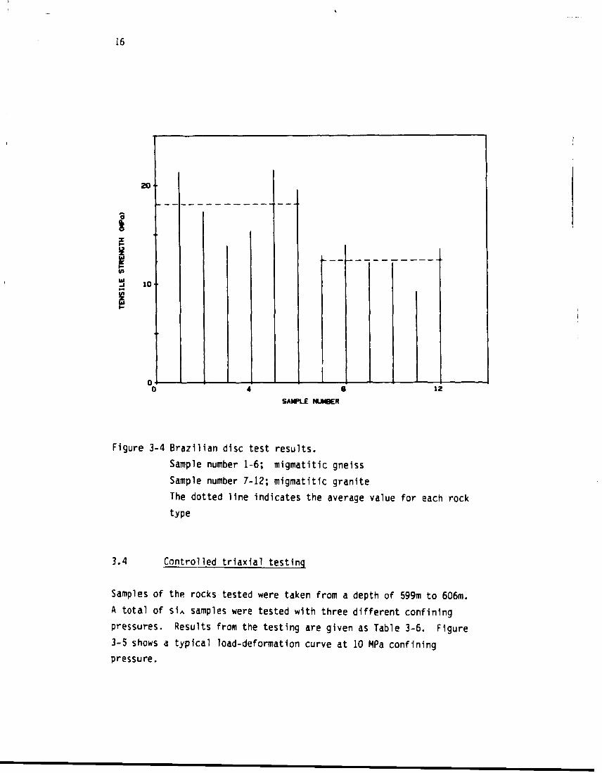
Figure 3-4 Brazilian disc test results.
Sample number 1-6; migmatitic gneiss
Sample number 7-12; migmatitic granite
The dotted line indicates the average value for each rocktype
3.4 Controlled triaxial testing
Samples of the rocks tested were taken from a depth of 599m to 606m.A total of six samples were tested with three different confiningpressures. Results from the testing are given as Table 3-6. Figure3-5 shows a typical load-deformation curve at 10 MPa confiningpressure.
17
200-
100'
.2 .4DEFORMATION ••
.e
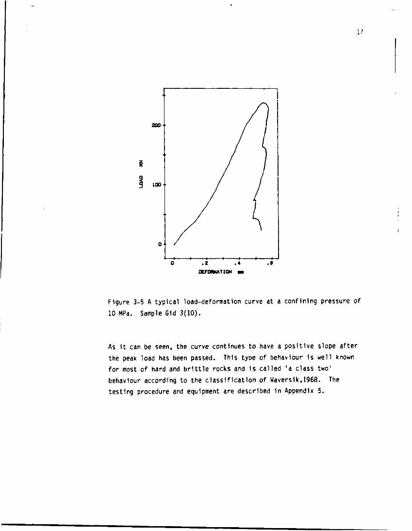
Figure 3-5 A typical load-deformation curve at a confining pressure of
10 MPa. Sample Gid 3(10).
As it can be seen, the curve continues to have a positive slope after
the peak load has been passed. This tyDe of behaviour is well known
for most of hard and brittle rocks and is called 'a class two'
behaviour according to the classification of Waversik,1968. The
testing procedure and equipment are described in Appendix 5.
18
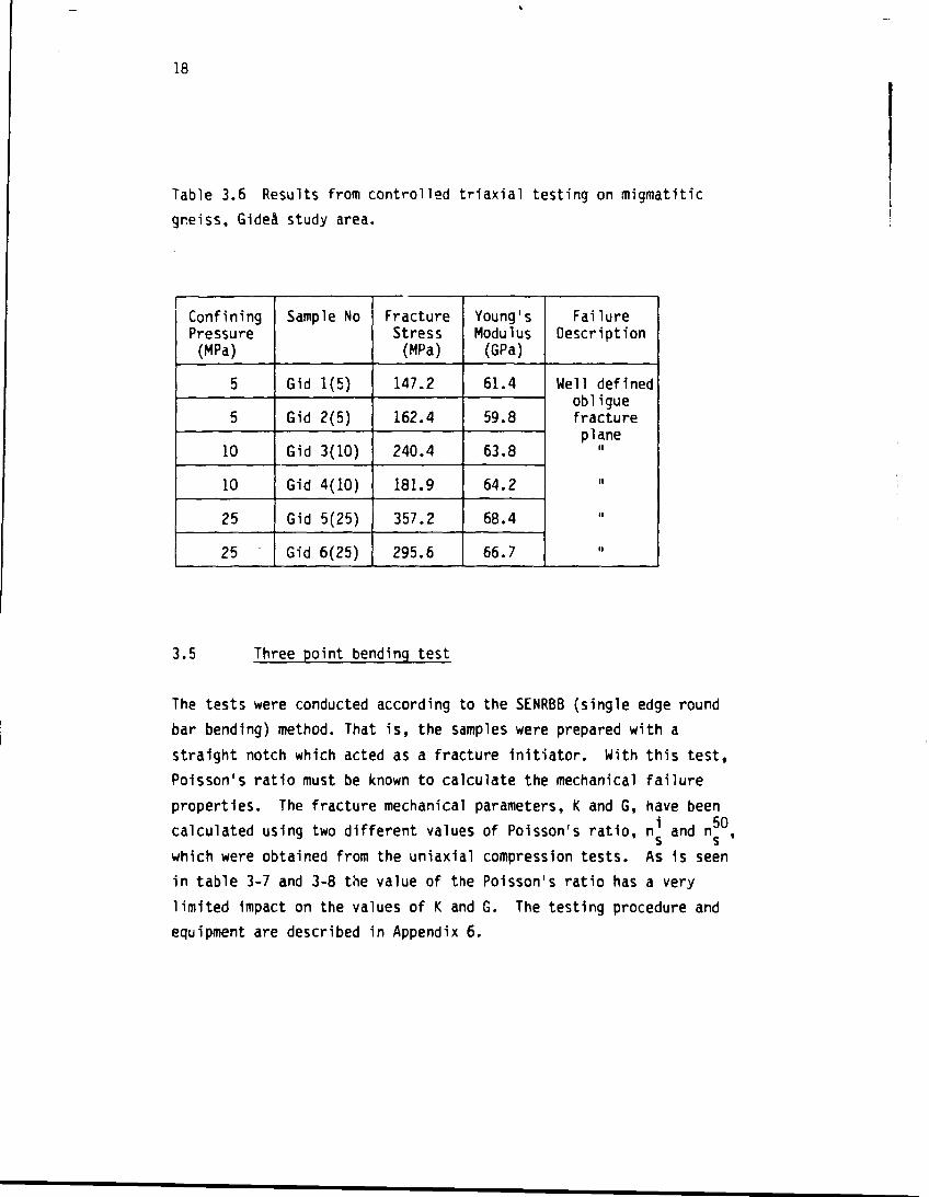
Table 3.6 Results from controlled triaxial testing on migmatitic
gneiss, Gideå study area.
1ConfiningPressure(MPa)
5
5
10
10
25
25
Sample No
Gid 1(5)
Gid 2(5)
Gid 3(10)
Gid 4(10)
Gid 5(25)
Gid 6(25)
FractureStress(MPa)
147.2
162.4
240.4
181.9
357.2
295.6
Young'sModulus(GPa)
61.4
59.8
63.8
64.2
68.4
66.7
FailureDescription
Well definedobliguefractureplane
•i
n
3.5 Three point bending test
The tests were conducted according to the SENRBB (single edge round
bar bending) method. That is, the samples were prepared with a
straight notch which acted as a fracture initiator. With this test,
Poisson's ratio must be known to calculate the mechanical failure
properties. The fracture mechanical parameters, K and G, have been
calculated using two different values of Poisson's ratio, n^ and rr ,
which were obtained from the uniaxial compression tests. As is seen
in table 3-7 and 3-8 the value of the Poisson's ratio has a very
limited impact on the values of K and G. The testing procedure and
equipment are described in Appendix 6.

table 3-7 Three point bending test results, Gideå
Calculations conducted with v.
19
Rocktype
Gneiss 1
2
3
4
" 5
6
AverageStd.dev.
Granite 1
2
3
4
5
6
AverageStd.dev.
(mm)
41.5
41.5
41.6
41.3
41.5
41.4
41.6
41.6
41.5
41.5
41.5
ao_
0.241
0.241
0.240
0.242
0.241
0.242
0.240
0.240
0.241
0.241
0.241
E-mod
(GPa)
55.5
53.9
46.6
60.3
27.7
63.1
51.2±12.8
63.4
60.9
52.7
46.5
36.9
52.1±10.8
a
4
0.349
0.331
0.276
0.393
0.359
0.335
0.355
0.371
0.367
0.330
0.394
max(kN)
2.33
2.29
1.69
2.18
1.35
2.77
2.10±0.50
3.11
3.19
2.89
2.40
1.95
2.71±0.52
K
(MN/m3/2)
2.083
1.951
1.241
2.228
1.241
2.394
1.86±0.50
2.819
3.025
2.722
2.039
1.985
2.52±0.48
G
(J/m2)
77.3
69.8
32.7
81.3
54.9
89.8
67.6±20.8
124.3
149.0
139.5
89.2
106.4
121.7±24.3

20
Table 3-8 Three point bending test results, Gideå
Calculations conducted with v_
Rocktype
Gneiss 1
2
3
4
5
6
AverageStd.dev.
Granite 1
2
3
4
5
6
AverageStd.dev.
*
(mm)
41.5
41.5
41.6
41.3
41.5
41.4
41.6
41.6
41.5
41.5
41.5
*
0.241
0.241
0.240
0.242
0.241
0.242
0.240
0.240
0.241
0.241
0.241
E-mod
(GPa)
55.6
54.0
46.7
60.4
27.8
63.2
51.3±12.8
63.4
60.9
52.7
46.6
37.0
52.1±10.8
a
*
0.354
0.334
0.276
0.400
0.363
0.338
0.362
0.380
0.377
0.334
0.401
max(kN)
2.33
2.29
1.69
2.18
1.35
2.77
2.10±0.50
3.11
3.19
2.89
2.40
1.95
2.70±0.52
K
(MN/m3/2)
2.110
1.967
1.241
2.269
1.256
2.413
1.88±0.50
2.879
3.105
2.793
2.064
2.031
2.57±0.49
G
(J/m2)
75.2
67.4
31.0
80.0
53.5
86.6
65.6±20.4
116.7
141.3
132.3
84.7
103.2
115.6±22.6

21
Q
a
O 20 40 60 80
LOAD POINT DISPLACEMENT (urn)
Figure 3-6 Typical recording from three point bending test.Migmatitic granite.

22
4 DISCUSSION
Primary and shear wave velocities for the Gideå rock types are high
for migmatitic gneiss and moderate for migmatitic granite when
compared with other Swedish granitic rocks. The microfracturing grade,
V /V , is typical for granitic rocks. It may also be pointed out that
the migmatitic gneiss has a higher dynamic elastic modulus than the
migmatitic granite. Results from the other tests (uniaxial
compression test and three point bending test) indicated the contrary.
A contributing factor is the higher density of the migmatitic gneiss,
as density is included in the calculation of the elastic moduli from
the sound velocity measurments. It is also notable that the
migmatitic gneiss has the lowest compressive strength, o , but the
highest tensile strength, (oj. This may be attributed to the mineral
composition and shape of mineral grains. There is a clear shape
orientation of the mica minerals in the migmatitic gneiss, and this
has probably had some effect on the test results.
The tensile strength of the migmatitic gneiss is high while that of
the migmatitic granite is around average for granitic rock types in
Sweden. The compressive strength, o , determined from uniaxial
compression testing for migmatitic granite (201 MPa) is clearly
comparable to that of Stripa granite (205 MPa) and considerably higher
than Bohus granite (157 MPa). Compressive strength of the migmatitic
gneiss for Gideå is considerably lower (128 MPa). This is most likely
due to its higher mica content. Plans cutting through a large number
of mica crystals tend to act as weakness planes.
The brittleness of the migmatitic granite is comparable with that of
the Stripa granite, whereas that of the gneiss is higher. Previous
studies (Ljunggren, Norin, 1985), indicate however, that an increase
in mica content has a damping effect on the registration of acoustic
events.
Results from the controlled triaxial test show an increase in failure
stress from 10 MPa to 25 MPa confining pressure. In particular, at
25 MPa confining pressure, the failure stress approaches a value which

23
is double that arrived at from uniaxial testing. Due to material
variation and the limited number of samples tested, it is not possible
to distinguish any change in failure stress up to 5 MPa confining
pressure.
Young's moduli obtained from these tests are consistent with those
obtained from uniaxial testing. Although a slight increase of the
moduli may be expected as a result of confinement, this cannot be
shown due to the limited number of samples tested.
To classify the results of the testing as objectively as possible, and
to ascertain whether the strength values could be regarded as weak or
strong, we have chosen to compare them with a compilation of
parameters for crystalline rock types conducted by Tammemagi and
Chieslar (1985). Information on Swedish rock types ((Swan, 1977) and
(Swan, 1983)) is also found in thi*; work. We have chosen to
re-present their data here and, at the same time, indicate where the
results from the Gideå rock types appear.
As is seen in Figure 4-1, the density values obtained from the Gideå
rock types fall well within the area that can be regarded as normal
for acid igneous rocks.
The compiled data on the elastic moduli exhibit a much larger standard
deviation than what is found in the density data. The reason for this
lies partly in the variety of test methods used and partly in the
different evaluation methods. The results, however, give and adequate
picture of the interval within which the elastic moduli normally are
located.

24
30-
25-
20-
UJ_ i£L
<
O
is-
le-
iUj UJ
o o5 o
1 IJ
MEAN-2700 kg/m3
STD. DEV.-150 kg/m 3
I 12300 2400 2500 2600 2700 2800 2900 3000 3100 3200
DENSITY (kg/m 1 )
Figure 4-1 Frequency histogram of density of crystalline rocks. 104samples. Gideå results are indicated by the arrows. (After Tammemagiand Chieslar, 1985).

UJ
W -
13 -
12 -
11 -
10 "
9 "
• -
7 -
a.* 6inu. 5
3
2
1
_ Jl
iri
t </>Z £
UJ UJ
9 9
II
Lfcz H2UJ< < UJ
oo oo
UJUJ UJUJ99 -99oo oo
o o
UJUJ
oo.5O O O O O
ii ii Ii
MEAN • 54,9 GPö
STD. DEV.. 18,9 G Po
nn10 20 30 40 50 60 70
YOUNG'S MOOULUS (GPa )
80 90 100
Figure 4-2 Frequency histogram of Young's modulus for c rys ta l l ine rocks. 160 samples. Results from
Gideå are indicated by the arrows. (After Tammemagi and Chieslar, 1985).
noCJl

26
As is seen in Figure 4-2, the initial elastic moduli, obtained from
uniaxial compression testing, E^, are markedly different from the
others. This is probably due to closing of microcracks and collapsing
of aspherical pores. Part of the measured strain is then a result of
rigid translation and rotation of crystals instead of true distortion
of crystal lattices. The calculated elastic modulus will then be
smaller at very low loads than at loads above which microcracks and
some pores have closed. In general, the elastic moduli from the Gideå
rock types lie in the vicinity of the average for the entire comp-
ilation, with the migmatitic granite having a somewhat higher value.
Poisson's ratio depends on which test and evaluation method was used
to obtain the result. Generally speaking, it can be concluded that
the Gideå results fall well within the area that is considered normal
for crystalline rock types.
The large standard deviation (81.6 MPa) is clear evidence of the large
variation that is present in the uniaxial compressive strength
determinations. As is seen in Figure 4-4, there is an obvious maximum
at around 200 MPa. Migmatitic granite can be taken as having a
moderate average value of compressive strength while migmatitic gneiss
has a considerably lower strength.
The determination of tensile strength of intact rock is a complex
task. Laboratory tests invariably indicate that ten?ile strength
depends upon sample size (the larger the sample, the lower the
strength) and upon the testing method utilized. Some of the methods
used for the determination of rock tensile strength are: direct
tension test, Brazilian disc test, and hydraulic fracturing. Even if
only one method is utilized, the data shows a large scatter about the
mean. Keeping this in mind, it is, however, apparent that the tensile
strength values of the Gideå samples, especially the migmatitic
gneiss, are quite high.

Figure 4-3 Frequency histogram of Poisson's ratio for crystalline rocks. 121 samples. Results from
Gideå are indicated by the arrows. (After Tammemagi and Chieslar, 1985).

IS -
u -
13 -
12 '
11 -
K) -
9 -to
!U •z< 7 -U.'
° 6-i
5 •
4
3
2
so
00
nnUJ
o
If
LnMEAN • 196,0 MPQ
STD. DEV.- 8t,6 MPQ
UJ
oI
Ui
z<o
<oo JLJ
100 150 200 250 300 350 400
UNCONFINED COMPRESSIVE STRENGTH ( M P Q )
450 500
Figure 4-4 Frequency histogram of unconfined compressive strength for crystalline rocks. 127 samples.
Gideå results are indicated by the arrows. (After Tammemagi and Chieslar, 1985).

5 -
UJ
g 3
g
1 -
MEAN-8,0 MPa
STD. DEV • 3,9 MPa
•f-6 8 10 12
APPARENT TENSILE STRENGTH I MPQ )
z
o
(/tV)
tu
O
o
Figure 4-5 Frequency histogram of apparent tensile strength for crystalline rocks. 39 samples. Gideåresults are indicated by the arrows. (After Tammemagi and Chieslar, 1985).

30
The fracture toughness, K. , which is described as the rock's
resistance to fracture propogation, is seen to be normal for
migmatitic gneiss when compared to other crystalline rock types. The
migmatitic granite, which has a K, =2.52 MN/m3/2 is somewhat more
fracture resistant than what is considered normal for granitic rock
types (see Table 4-1).
Table 4-1 Fracture toughness for granitic rock types
Rocktype
Migmatitic gneiss, Gideå
Migmatitic granite, Gideå
Granite, Öjebyn
Quartzite, Kiruna
Stripa granite
Avesta gneiss
Klc
(MN/m3/2)
1.88
2.52
1.411
2.282
1.983
1.94"
1 Obtained from results reported by Lindqvist and Rånman (1980)2 Alm (1983)3 Sun (1983)4 Ljunggren, Norin (1985)
A final evaluation of the characteristics of the tested rock types is
that the migmatitic gneiss has varying strength properties. What is
especially obvious is its low compressive strength in comparison to
its high tensile strength. Petrographic studies indicate that the
minerals which compose the material have a preferred shape orientation
and that the content of mica is significant. The latter factor has a
negative effect on the compressive strength. Migmatitic granite,
however, may be classed as having average values (c.f. Tammemagi and
Chiesiar, 1985). No data from Gideå can be regarded as abnormal.

31
5 RECOMMENDATIONS
To increase our knowledge of the mechanical characteristics of Swedish
rocks, and in particular those that eventually will be targets for
further development for a nuclear waste repository, it is important to
test the rock types that appear in the other study areas.
A problem that always confronts the investigator is that testing is
conducted on fresh, intact rock whereas the excavation is carried out
in a rock mass which in addition contains fractures, joints and joint
fillings. Elastic and fracture mechanical properties of intact rock
are there- fore not the same as those of a rock mass. Hence a more
complete study of rock mass characteristics must incorporate studies
of joint properties as well as the properties of the joint filling
materials. Studies along these lines are recommended before any final
design of the repository is made. A more comprehensive study of the
properties of the intact rock is also necessary.
Direct experimental studies of rock mass properties are difficult to
carry out. Nevertheless such results are of vital importance if a
better understanding of the behaviour of the rock mass is to be
reached. Large scale testing offers interesting prospects in this
case. A great step towards controlled experimental studies of rock
mass properties would be taken if specimens having dimensions of
approximately lxlxl m could be tested. Large scale laboratory testing
are therefore recommended for future research.

32
REFERENCES
[1] Albino B, Nilsson G, 1982. Sammanställning av tekniska data för
de olika borrhålen samt sprick- och bergartsloggar,
typområdet G Idea. KBS ARBETSRAPPORT AR 84-23.
[2] Albino B, Nilsson G, Stenberg L, 1982. Geologiska och geofysiska
mark- och djupundersökningar. KBS ARBETSRAPPORT AR 83-19.
[3) Alm 0, 1983. Results from Mechanical Testing of Six DifferentRock Materials. Internrapport BM 1983:05. 30p.
[41 Hakami H, 1985. Cast On Rock Inclusion Gauged Sleeve for
Controlled Uni-axial and Tri-axial Compression Tests onRocks. A progress report, Internrapport BM 1985:01.
[51 ISRM, 1981. Rock Characterization Testing and Monitoring. ISRM
Suggested Methods. Brown E T (Ed). 211 p.
[61 KBS-3. Använt kärnbränsle-KBS-3. II Geologi. SKBF/KBS.
[7] KBS-3: Använt kärnbränsle-KBS-3. IV Säkerhet. SKBF/KBS.
[81 Lindqvist P-A, Rånman K-E, 1980. Mechanical Rock Fragmentation;
Chipping Under a Disc Cutter. Technical Report 1980:59 T,
University of Luleå, Sweden.
[91 Ljunggren C, Norin J, 1985. Akustisk Emission vid Bergarts-testning. Teknisk Rapport 1985:25 T, LuH, Sverige. 59p.
[101 Sun Z, 1983. Fracture Mechanics and Tribology of Rocks and
Rock Joints. Doctoral Thesis, 1983:22 D, LuH, Sweden. 207p.

33
[111 Swan G, 1977. The Mechanical Properties of Rocks in Stripa,Kråkemåla, Finnsjön and Blekinge. KBS-48, prepared forKärnbränslesäkerhet, Stockholm, Swedan.
[12] Swar, 6, 1978. The Mechanical Properties of Stripa Granite.
Tecnical Project Report No. 3. Originally part of KBS
Teknisk Rapport 48, Kärnbränslesäkerhet (KBS), Sweden. 25p.
[13] Swan G, 1983. Determination of Stiffness and Other Joint
Properties From Roughness Measurments, Rock Mechanics andRock Engineering, Vol. 16, pp. 19 - 38.
[14] Tammemagi H Y, Chieslar J D, 1985. Interim Rock Mass Properties
and Conditions for Analyses of a Repository in Crystalline
Rock. Technical Report BMI/OCRD-18. 84p.
[15] Wawersik W R, 1968. Detailed Analysis of Rock Failure in
Laboratory Compression Tests. Ph.D Thesis, Unversity of
Minnesota.
APPENDIX 1
DETERMINATION OP SOUND VELOCITY AND OYNAMICPARAMETERS OF ELASTICITY FOR ROCK SPECIMENS
Introduction
The easiest way to study the dynamic properties of rock specimens
is by means of ultrasonic sound velocity measurements. In an iso-
tropic material the velocity of the shear waves, V and the
compression waves, V is the same in all directicns. If the material
is linearly elastic the elastic parameters of the specimen can be
calculated from the measured velocities, V and V .
Experiments have shown that the velocity of elastic waves in a rock
material depends both on the mineral composition of the rock and
its porosity and content of microfractures. The specimens degree
of saturation does also have strong influence on the sound velocities.
Sound velocity measurements, in combination with microscopic analysis,
can be used to study the porosity of rocks.
The main purpose of the test is to determine the elastic properties
of the specimen. This is done within the elastic loading range of
each rock type.
Equipment
The equipment for measuring sound velocity in rock specimens include
the following components:
a) Two cylindrical transducers (* 50 x 50 mm), each containing two
piezoelectric crystals - one for shear waves,S the other for com-
pression waves, P. Both crystals having own frequency of 1 MHz.
The transducers can take an eavenly distributed compressing load
of 220 kN, equaling 112 MPa stress

b) Pulse generator/measuring unit, type PUNDIT
c) Oscilloscope with memory, type GOULD 4000
d) Switch unit to switch between P and S crystals
e) X-Y recorder to plot from the oscilloscope memory
f) Loading machine for loading specimen and transducers to acertain
good rock-transducer contact. An INSTRON 10 ton servo-hydraulic
press serves this purpose.
g) Spherical seat for eaven load distribution on transducers and
specimen
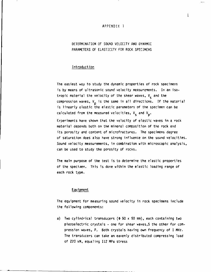
Figure 1 shows the principles of component layout for the test.
Fig. 1 The layout of components for measuring sound velocity
in rock specimens.
Sample preparation
In a standard test the sound velocities, Vp and Vs, are measured
in rock specimens of straight circular cylinders. Other sample
shapes are possible but the specimen must have two parallel and
planar surfaces for placing the transducers on. It is common
to do sound velocity measurements on specimens prepared for uni-
axial compression test. These specimens meet all requirements
set on sample preparation for sound velocity tests. Test specimens
from drill cores are prepared in the following way:
a) Cylindrical specimens with parallel end surfaces are cut with
a diamond blade. The ends shall not depart from perpendicularity
to the axis of the specimen by more than 4 min or 0.05 mm over
a specimen of 50 mm diameter. As a standard we have chosen a
specimen length of 2.5 times it's diameter. The length to dia-
meter ratio should not be less than 2. An eventual departure from
this rule shall be noted in the test report.
b) After cutting the specimen it is dried in oven at 50° C for a
minimum period of 24 hours. The specimens are stored in a
desiccator till the time of testing.
If a specimen is to be tested in a saturated state it must
lie submerged in water for at least 24 hours before testing.
If a specimen has started drying it shall be placed in vacuum
to get rid of air in pores, preventing water to enter. After
de-airing the specimen it is submerged in water while still in
vacuum. The procedure is called vacuum impregnation.
Specimens to be tested at normal laboratory humidity shall standuncovered in the laboratory for one week at least.

Test procedure
The piezoelectric crystals are embedded in the steel cylinders of the
transducers. While traveling between crystals on opposite ends off
the specimen a sound wave must therefore pass through two layers of
steel of unknown thickness plus the specimen. Before running the test
we need to know the travel time of sound waves through these steel
layers. This is done by placing the transducers against each other,
with two pieces of double aluminium foil between, those sitting at the
ends of the specimen during normal testing. The travel time through
the tra;.. .iucer system is now measured in usual way. This procedure
is called zero-reading. The travel time obtained in the zero-test
will be subtracted from the total travel time during normal rock
specimen testing.
Specimen and transducers must be loaded to give good acoustic contact.
Experiments have shown that 5 MPa stress is sufficient to aquire good
contact between specimen and transducers (see Fig. 2). ISRM's
"Suggested Methods" (Brown 1981) recommend 0.1 MPa but this stress is
to low for our type of transducers.
For soft rock or fractured the stress may be reduced from 5 MPa
down to 3 MPa for example. In such case it should be noted in the
test report. The measurements are run in the following way:
a) Components are connected and tested
b) Zero-reading is carried out. Travel time through the zero-system
is measured both for P and S waves
c) A rock specimen, with double aluminium foil covering each end, isnow placed between the transducers

d) Specimen with transducers is now placed on a spherical seat in
the press and centered carefully. The spherical seat will
contribute to an eaven load distribution in the system. Speci-
men and transducers is now loaded to 5 MPa
e) The test is run at 5 MPa axial stress. The equipment are con-
nected in such a way that the pulse activating the transmitting
crystal will also trigger the scanning of the oscilloscope. The
scanning time is chosen to give good resolution over the period
from transmitting to receiving the wave. The curve on the
oscilloscope is recorded by an internal memory for later plotting
it on paper by a recorder working in X-t mode. The memory can
save one curve at a time. Figure 3 shows typical curves for P-
and S-waves and how the traveling time for these is determined.
The time difference between the points on the curve is 0.55 us.
Calibration of the time axis on the paper plot is achieved by
measuring the distance between points n and n + 50
f) The load is now decreased down to axial stress of 1 MPa. Measure-
ments are repeated at this stress level
g) New double aluminium foils are placed on the ends of the specimen
and points c) to f) repeated
h) Travel times through the specimen for P-waves, t* and S-waves, tt
are found as the difference between total travel times, t and t
respectively and the zero-times, t° and t° e.i.
t; • tj - t°
Where t , t , t° and tQ are average values from two measurements.

o
o_ i
UJ
oV)
AXIAL LOAD
Fig, 2 Sound velocity as a function of axial stress for cylindrical
specimens of Stripa Granite.

CALIBRATIONinLUCL
ti
ö
COin
CL
tiX
12.21 us
L7.S9JJS
,., 12.09 us,.
12.09JJS_
n
.̂28 us.
P.+50
ininLU
cr
ROCK-- Stripa granite
38.62 us
Ts= 26.53 us
n+50
io
2A.69 us
Tp= 17.41 us
n+50
Fig. 3 Typical plots from P- and S-waves in Stripa Granite.

Calculations
For calculating the sound velocities the specimen length must be
known. In our standard tests we measure the length, L the diameter,
D and the weight, m of the specimen. The value presented for each
parameter is an average from several measurements.
Sound velocities are calculated from equations (1) and (2):
P-wave velocity V. = L/t: (1)
S-wave velocity = L/t" (2)
If the rock material is taken to be linearly elastic and isotropic
the elastic parameters can be calculated straight foreward. Young's
modulus, E. and Poisson1s ratio, v. are then found from equations (3)
and (4):
Young's modulus
Poisson's ratio
Ed =
Vd = 2
(3)
(4)
The bulk modulus, B . and the shear modulus, G . are found through
the relationship between E, u, G and B. Equations (5) and (6) give
B and G as functions of E and u.

B = 3(1 - (5)
G = 2(1 + v) (6)
Reporting of results
The results are listed in a table (see Table 1) and in a sample-
comparison diagram (Fig. 4). Visible structures in specimens are
noted in the Comment column.
Table 1 Results from sound velocity measurements, average valuesfrom two measurements.
Rock
type
Sample
nr
L
(mm) (mm)
m
(g)
P
(kg/m3)VP(m/s)
V
(m/s)
Ed(GPa)
vd(m/s)
Comments

10
6000-
5000-
•Z 4000-oo
» 0 0 -
2000-
1500- I
L"8
II
LOAD: MPo
• \ '
1v vy vi
i-x ̂<IÉ
SAMPLE NR
SHEAR WAVE VELOCITY, Vs (m/s)
COMPRESSION WAVE VELOCITY, Vp
E-MODULUS,(GPa)
POISSON'S RATIO
Fig. 4 Sample comparison diagram for each specimen showing: V
(m/s), V (m/s), Young's modulus (GPa) and Poisson's ratio.
References
Brown, E. T. (ed) 1981. ISRM Suggested Methods. Rock Characterization,
Testing and Monitoring. Suggested Methods for Determining Sound
Velocity. Pergamon Press, Oxford.

APPENDIX 2
UNIAXIAL COMPRESSION STRENGTH, MODULUS OF ELASTICITY
AND POISSON'S RATIO
This testing method serves to determine the modulus of elasticity,
the Poisson's ratio and the uniaxial compression strength of intact
rock samples. The test specimen is made of a rock cylinder with the
ends cut perpendicular to the axis of the cylinder and polished for
a high degree of parallelity. This is a standard test for determining
mechanical properties of rocks.
Equipment
a) The test is run in a servo-hydraulic Instron press with loading
capacity of 4500 kN and a maximum piston movement of + 35 mm. The
loading rate can be set within wide limits. The stiffness of the
press is sufficiently high to neglect it's effect on the test
result
b) Cylindrical platens of high quality steel are placed on both ends
of the specimen. The diameter of the platens is D to D+2 mm,
where D is the diameter of the specimen and the minimum thickness
should be at least 15 mm or D/3. Surfaces of the platens should
be ground and their flatness should be better than 0.005 mm
c) One of the two steel platens contains a spherical seat. The
spherical seat must be cleaned thoroughly and lubricated by
a few drops of mineral oil before placing it under the specimen.
The specimen, the steel platens and the spherical seat must be
accurately centered in the press before starting the test
d) Strains in the specimen during the loading cycle are measured by
strain gauges. If strains are measured by some other method
it's reading limits should be 5 x 10⁻⁶ strain at least.

Recommended effective length of strain gauges is 10 times the
biggest grain size of the rock sample with an upper limit at half
the diameter of the specimen
e) Recording of strain and load during the test may either be done
by a conventional X-Y recorder or a computer
« = STEEL PLATEB = "0C< ?/>MPLEC = SPHERICAL SEAT0 = APFLIFD AXIAL
Fig. 1 Example of an experimental set-up.
Procedure
a) The rock specimen is a straight, circular cylinder with a length
to diameter ratio of approximately 2.5. Smaller sample diameter
than 40 mm should be avoided
b) The ends of the specimen shall be flat to 0.02 mm and shall notdepart from perpendicularity to the axis of the specimen by morethan 0.05 mm

c) The sides of the specimen shall be smooth and free from abrupt
irregularities. A specimen that does not ful Ifi 1 the above
listed rules on specimen quality shall not be tested as it might
affect the test results
d) The diameter of the test specimen shall be measured to the nearest
0.1 mm. Three measurements shall be taken and averaged. The ave-
rage is used to calculate the cross-sectional area of the speci-
men. The specimen length is measured to the nearest 0.1 mm.
Specimen weight is determined tc calculate it's density. The
weight should be measured to the nearest 0.1 g for specimen dia-
meter of 40-80 mm
e) The axial loading rate should be set to reach specimen failure
within 5 - 1 0 minutes. Alternatively a constant stress rate
can be set between 0.5 - 1.0 MPa/s
f) The maximum load on the specimen shall be recorded in Newtons
(or an appropriate multiple thereof) to within 1 %. The de-
formations in the specimen are recorded in strains or a multiple
thereof. The most common unit is the micro strain (us)
g) As a compliment to the standard method of testing the registration
of acoustic emission from the specimen can be acieved. This has
shown to give valuable information on the initiation of failure
in the specimen
h) The minimum number of specimens tested for each rock type should
be five

Calculations
a) Axial strain is calculated from the equation:
_ Alea = l0
where t, = Axial straind
1Q = Initial axial length of specimen
Al = Change in measured axial length
b) Radial strain is calculated from the equation:
d0
where e = Radial strain
do = Initial diameter of specimen
Ad = Change in diameter
c) The axial stress in the specimen (a) calculated from the equation:
where o = The compress i ve stress
F = The axial force
A = The initial cross-sectional area of the specimen
The uniaxial compression strength (oc) is calculated from the
above equation from the maximum load on the specimen (F_.J.
d) A typical plot from this test is shown in Fig. 2. The curvesshow axial stress vs. axial and radial strain in the specimen.

The diagram shows a typical behaviour of rock material through
the applied stress range.
O
Fig. 2 Example of a graphical presentation of axial and
radial stress-strain curves.
e) The modulus of elasticity is calculated from the equation:
where E = The modulus of elasticity
Ao = Change in axial stressea = Change in axial straina
Various methods are accepted for calculating the modulus of elas-
ticity. Following methods are used at the Division of Rock Mechanics:

1) The tangent modulus (Et); calculated at 50 % stress level
of the uniaxial compression strength
50'/.e T = A£
Ea
Fig. 3 Calculation of the tangent modulus of elasticity.
2) The average modulus (Eflv); Calculated as the inclination
of the linear portion of the stress-strain curve.
aA
Or Ya iAe a
-•Ea
Fig. 4 Calculation of the average modulus of elasticity.

3) The secant modulus (E ); calculated as the inclination
of the secant line to the curve from 0 point up to a fixed
percentage, commonly 50 %, of the ultimate strength
. A Q
50V. —
Fig. 5 Calculation of the secant modulus of elasticity.
4) The initial modulus of elasticity (E. .); calculated as
inclination of the tangent to the initial part of the
curve.
it a
Fig. 6 Calculation of the initial modulus of elasticity.

The Young's modulus is presented in the Pascal unit (Pa)
or a multiple thereof. Commonly in GigaPascals (GPa).
f) The poisson's ratio (v) is calculated in the following way:
Inclination of the axial stress-strain curvev = Inclination of the radial stress-strain curve
E
Inclination of the radial curve
g) The volumetric strain (Ey) is calculated from the equation:
S = ea + 2er
Reporting of results
A report from the test should include the following:
a) A lithological description of the rocks tested, also givingsampling location and depth
b) Orientation of the axis of loading with respect to specimen
anisotropy
c) The test results shall be set up in a table, eventually completed
by a sample-comparison diagram showing the variation in com-
pressive strength between the specimens (se figs. 7 and 8)
Rock type Sample
nr
D
(mm)
L
(mm)
m
(kg)
p
(kg/m3)
Fmax(N)
o
(Pa)init(GPa)
E50V.in
V50Remarks
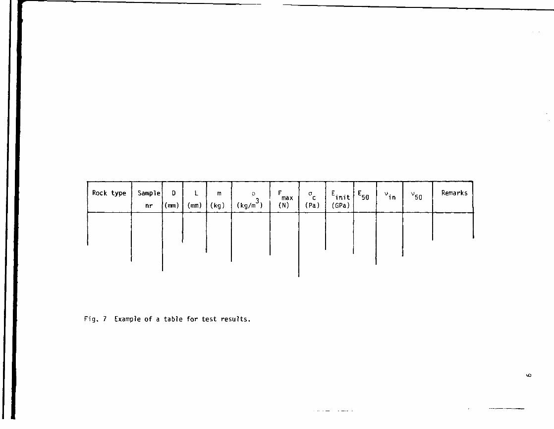
Fig. 7 Example of a table for test results.

10
Sample nr
1 8
Fig. 8 Example of a sample-comparison diagram showing the variationof compressive strength between specimens in the same series.
References
Brown. E.T. (ed) 1981. ISRM Suggested Methods. Rock Characteri-
zation, Testing and Monitoring. Suggested Methods for Determining
the Uniaxial Comnpressive Strength and Deformability of Rock
Materials. Pergamon Press, Oxford, 211 pages.
Jaeger, J.C. and Cook, N.G.W. 1979. Fundamentals of Rock Mechanics.Third edition. Chapmann and Hall, London, 593 pages.

APPENDIX 3
ACOUSTIC EMISSION
Scope
Acoustic emission are used as a help and complement to other test
methods wich are conducted at the Division of Rock Mechanics,
Technical University of Luleå. By the acoustic emissions one
registeres the sound waves caused by crack generation in a rock
sample. The acoustic emissions are used to get an idea about when the
cracks initiate and propagate. At the present the acoustic emissions
(AE) can be used as a routine in the following testing methods:
Uniaxial compression test, three point bending test, brazilian test,
as well as hydraulic fracturing and sleeve fracturing.
Apparatus
The equipment for acoustic emission consists of the following parts:
1) Transducer: A piezoelectric transducer which is in contact with the
sample and transforms the sound waves of the microcracking into
electrical signals.
2) Pre-amplifier: It is placed near the transducer and transfers the
signal to the counter. The amplification is +60 dB.
3) Filter: It filters out mechanical (low frequence) and electromag-
netic disturbances. The signals which are significant for rock are
within the frequency range 100 kHz - 1 MHz.
4) Amplifier: It amplifies the signal even more. The amplification can
be varied between 0-60 dB in steps of 1 dB.
5) Threshold detector: The instrument reads the signal and only
releases the peaks which pass over a pre-set threshold value.
6) Counter: Counts the number of pulses that have passed t.ie thresholddetector.

Besides, a printer can be connected, which will then show the
acoustic emissions.
Procedure
The AE equipment is connected according to the block diagram below,Fig 1:
TRANS- PREAM- FILTER AMPLIFIER THRESHOLD" COUNTERDUCER PLIFIER DETECTOR
Fig 1 Block diagram for AE equipment.
The transducer (phone) is placed as close as possible to the sample,
but not so near that eventual rock splinters can damage it. In
uniaxial compression test, the transducer is placed in a specially
constructed holder so that it is well protected. The holder is placed
directly under the sample. Between the metal surface and the transdu-
cer is applied a thin layer of vacuum grease. This is to improve the
transfer of signal to the measuring instrument and to avoid the re-
gistration of not wanted signals.
A micro-computer of type ABC 800 is connected to the counter for
the collection of the acoustic emissions during the test. The
frequence interval is set to 300 kHz - 1 MHz.
Calculations
The acoustic emissions do not give any value of a rock's strength orelastic paramenters. AE shall be seen as a complement to the othertesting methods. What AE can show is how fast and at which load thecracks initiate and propagate.
Presentation of results
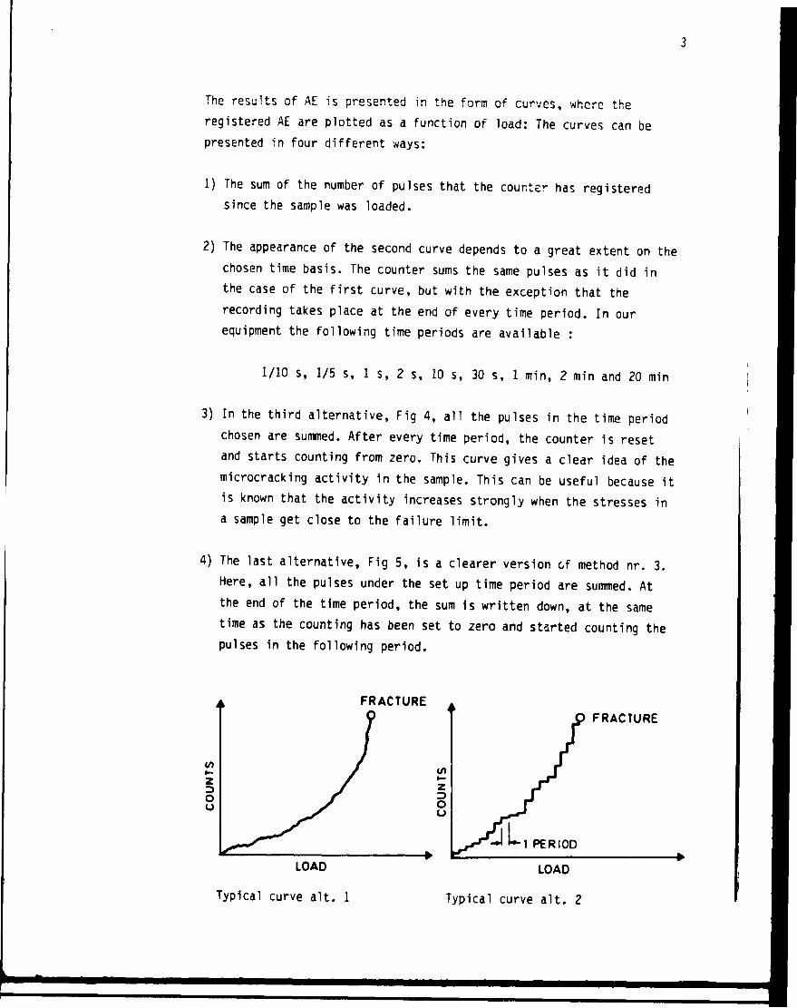
The results of AE is presented in the form of curves, where theregistered AE are plotted as a function of load: The curves can bepresented in four different ways:
1) The sum of the number of pulses that the counter has registeredsince the sample was loaded.
2) The appearance of the second curve depends to a great extent on thechosen time basis. The counter sums the same pulses as it did inthe case of the first curve, but with the exception that therecording takes place at the end of every time period. In ourequipment the following time periods are available :
1/10 s, 1/5 s, 1 s, 2 s, 10 s, 30 s, 1 min, 2 min and 20 min
3) In the third alternative, Fig 4, all the pulses in the time period
chosen are summed. After every time period, the counter is reset
and starts counting from zero. This curve gives a clear idea of the
microcracking activity in the sample. This can be useful because it
is known that the activity increases strongly when the stresses in
a sample get close to the failure limit.
4) The last alternative, Fig 5, is a clearer version of method nr. 3.Here, all the pulses under the set up time period are summed. Atthe end of the time period, the sum is written down, at the sametime as the counting has been set to zero and started counting thepulses in the following period.
zoo
FRACTURE
LOAD
Typical curve alt. 1
Z
Oo
1 PERIOD
FRACTURE
LOAD
Typical curve alt. 2

FRACTURE
LOAD H h 1 PERIOD
Typical curve a l t . 3
.n n
FRACTURE
LOAD
Typical curve alt. 4
Fig 2 Typical curves for the different registering alternatives.
References
Ljunggren, C. 1984. Laboratoriebestämning av bergarters draghåll-
fasthet med hydraulisk spräckning och membranspräckning.
Examensarbete 1984:078 E. Högskolan i Luleå, Luleå.
Ljunggren C, Norin J, 1985. Akustisk Emission Vid Bergartstestning.
Teknisk Rapport 1985:25 T. Högskolan i Luleå, Luleå.

APPENDIX 4
DETERMINATION OF INDIRECT TENSILE STRENGTH WITH BRAZILIAN TEST
Apparatus
a) A loading rig consisting of two steel plates loads a disc shaped
rock specimen diametrically, until failure occurres, see Fig 1. The
dimensions of the parts of the loading rig are the following: The
radius of the steel plates is 1.5 x the radius of the specimen, the
guide pins permit a rotation of one jaw relative to the other by
4 x 10 radians out of plane of the apparatus. The width of the
jaw is 1.1 x the specimen's thickness. The upper steel plate (jaw)
has a spherical seat to avoid inclined loading.
b) A servo-hydraulic Instron press is used to load the specimen in a
control led manner.
c) An X - Y recorder is used to register the load.
Spherical seat
Upper jaw
Guide pin
Test specimen
Lowerjaw
Fig 1 Loading equipment for Brazilian test.

Procedure
a) The specimen is cut, so as to provide parallel ends.
b) The diameter of the specimen is normally 42 mm, and the thicknessis chosen to be 0.5 x the diameter.
c) The orientation of the specimen shall be known and is given in the
results table.
d) The specimen is placed so that the load is applied diametrally.
e) The loading rate is chosen so that failure occurres within 15 - 30
seconds.
f) The load is registered continously on the X - Y recorder, and the
failure load is estimated.
g) The number of samples varies depending on the practical circumstan-
ces. Since the results often show a large spread, the number of
specimens should be at least 10 for each rock type.
Calculations
The tensile strength, ot, is calculated with the following formula:
ot = 0.636 P/D x t (MPa)
where P = failure load (N)
0 = diameter of the specimen (mm)
t = thickness of the sample (mm)
Presentation of results
a) Description of specimen location and depth.
b) Geological description of the rock type.
c) Orientation of anisotropy or foliation in relation to the direction

of the load.
d) Description of the failure appearance for each specimen.
e) Tests results are presented tabulated, according to Table 1
Table 1 Tensile strength by Brazilian test method.
Rocktype
Samplenr
Diameter
0[mm]
Thickness
t[mm]
Mass
m
[gl
Density
P[kg/mJ]
Max load
max[Nl
Tensilestrength
°1[MPa]
Remarks
References
Mellor, M. och Hawkes, I. 1971. Measurement of tensile strength bydiametral compression of disces and annul i. Eng Geol, i5, pp173-225.

APPENDIX 5
CONTROLLED TRI-AXIAL COMPRESSION TESTING
Purpose
It is known that natural rock formations are in a tri-axially state ofstress. Knowledge of the strength of rock under such state is veryimportant for designing structures in rock.
By conducting conventional tri-axial tests, it is possible to obtainthe strength of rock under different confinements. These data furtherhelp us to determine the strength envelope and calculate the internalfriction angle (*) and apparent' cohesion (c) of the rock material.
Controlled tri-axial testing, however, are more informative. They showus how rocks behave when their peak strengths have been passed and howreduction in load-bearing capacity takes place with the continuationof deformation.
Testing equipment
A high pressure cylindrical vessel, with a pressuring chamber dia-meter of 70 mm and height of 170 mm, made of handened steel is used.Strain gauge wires are connected to a specially designed collar, sit-ting at the bottom of the chamber. The teflon packing ring of the col-lar seals of the oil from leaking out. Details of the vessel andaccessories are found in Fig 1, schematically.
A pressure intensifier provides the necessary confining pressure andmaintains the pressure constant, while the specimen is being deformed.
The axial load on the sample is applied by the existing 4500 kN stiffand servocontrolled Instron testing machine. It is possible to carry-out the test in 'strain control' by this system. Details of thesystem is shown schematically in Fig 2.

12-
%, »' .'
-2<3
-5-6
-8
-9
Fig 1 Schematic view of the high pressure vessel, accessories andthe sample
1 - Pressurizing chamber2 - Top piston with two teflon
Packing rings
3 • Sperical seat
4 - Top platen
5 - Specimen
6 - Sleeve
7 - Inside wires
8 - Bottom platen
9 - Bottom collar with one
teflon packing ring
10 - Outside wires
11 - Body of the vessel
12 - Oil duct

Fig 2 Schematic view of the 4500 kN Instron Press
Fig 3 A prepared specimen for tri-axial testing

Specimen preparation
Samples of the rock to be tested, with diameter of 41.5 + 0.5 mm andlength to diameter ratio of L/D = 2 are prepared for testing. The pre-paration is exactly as that for uniaxial testning with longitudinaland circumferential strain gauges mounted on the specimen for strainmeasurements. The specimens are then prowided with 'Cast on RockInclusion Gauged Sleeves', so that controlled tri-axial testing can becarried out on them. Two long strain gauges are embedded in thesesleeves and provide the 'feedback' signal for the loading system.Details of the sleeve preparation is reported elsewhere (3). Fig 3shows a prepared specimen.
Testing procedure
The experiments are conducted in the following way:
- The specimen is placed in the pressurizing chamber, all thestrain gauge wires are connected and the chamber is filledwith oil.
By pushing the top piston into the chamber, the specimen is slightlyloaded, while no oil pressure is being built up.
- The confining pressure is raised to the desired value by thepressure intensifier.
- The loading of the specimen, then starts in 'position con-trol1, (see reference 2).
- At about 50% of the ultimate strength of the specimen, thecontrol is transferred to "strain controller1 module, wherethe long circumferetial strain gauges are responsible ofprowiding the "feedback1 signal for the system.
- The experiii.ant is continued in this manner until the com-plete load-deformation curve for the specimen is recorded.
Calculation of the elastic properties
Calculations of the fracture stress, modulus of elasticity, axial andradial strains are exactly as those for uniaxial testing.
Reporting of the results
A summary of the results may be reported in a table, an example ofwhich is given below.
SampleNo
Confiningpressure
MPa
FracturestressMPa
Young'smodulus
RPa
Failuredescription

REFERENCES
1) Brown E.T. (ed), 1981. ISRM suggested Methods, Rock Characte-rization, Testing and Monitoring.
2) Instron Manuals
3) Hakami Hossein, 1985. Cast on Rock Inclusion Gauged Sleeve forControlled Uni-axial and Tri-axial Compression Tests on Rocks.A progress report, Internrapport BM 1985:01.
4) Wawersile, W.R. 1968. Detailed Anlysis of Rock Failure in Labora-tory Compression Test. Ph.D Thesis, University of Minnesota.

APPENDIX 6
FRACTURE TOUGHNESS DETERMINATION WITH THREE POINTBENDING TEST
Scope
With this method it is determined a rock's modulus of elasticity, E,
and the stress intensity factor, K. , which is a measure of the stress
concentration at a crack tip. The three point bending test also gives
the energy release rate, G. The test can either be performed as a one
cycle test or as a several cycles test.
Apparatus
The experimental set-up is shown in Fig. 1. The experiment is conduc-
ted in a 10 ton servohydraulic Instron press, which is equipped with
a 1.5 ton load cell for registering the applied load. Downwards
flexure at the loading point is measured with two LVDT transducers
(Linear Variable Differencial Transformer). Widening of the crack is
measured with a COD gauge (Crack Opening Displacement). An X-Y re-
corder of type Hewlett Packard 7046A is used for registering load as
function of the average value of the LVDT transducers.
SECRBB configuration
Ftop roller
•clip gauge
Fig 1 Experimental set-up for three point bending test.

Procedure
a) The three point bending test is conducted on drill cores and the
ratio S/D shall be 3.33, where S is the c-c distance between the
support rollers and D is the diameter of the core.
b) At one half of the distance S is sawn a 0.8 mm wide and 10 mm deep
notch.
c) Tne supports for the COD gauge are glued on the sample.
d) Mounting of the measuring frame and the yoke on the sample.
e) The prepared sample is placed in the press.
f) A low load is applied to the specimen under load control, usually
0.1 KN.
g) Alignment of the specimen under load,
h) Mounting of COD gauge.
i) The measuring frame is controlled and adjusted.
j) Mounting of LVDT transducers as well as zero correction of the
signals.
k) A X-Y recorder is connected to the load signal as well as to the
LVDT signals.
1) The test is strain controlled via the COD gauge, with a strain rate
of 0.1 um/s.
m) The time for a test to total failure should not exceed 15 min.
Calculations
The calculations for a test with only one cycle are done according tothe following:

Step 1 Calculate the initial modulus of elasticity, E
X x E x D = g(a/D, v) = 15.6719(1 + 0.1372(1 + v) +
+ 11.5073 x (1 - v2)(a/D)2'5 x
x (1 + 7.0165(a/D)4*5)]
A6FA6Fwhere X = TF~ [mm/kN]
a = crack length [mm]. Here, it is set a = a
a = notch depth [mm]
D = diameter of the sample [mrnl
(1)
v - Poisson1s ratio
Fig 2 Diagram of load, F, as funtion of load point deformation,
for a test with one cycle.
Step 2 Calculate the real crack length, a, from equation (1) with an
iterative method. Use X from l_i and the modulus of elastici-
ty from the first calculation.
Step 3 Use a, given from step 2 to calculate the paramenter Y' in
equation (2)

Y" = 12.7527(a/0)0'5 [1 + 19.646(a/D)4-5]°'5/(l - a/D) 0 ' 2 5
(2)
Step 4 Calculate fracture toughness, K, with equation (3), where
F - F m a x (see Fig 2)
K = O.25(S/D) x Y" x F/D1.5 (3)
Wfiere K = K Secant fracture toughness [MN/m3/2]sec
Step 5 Calculate energy release rate, G
G = (1 - v2) x K2/E [J/m2] (4)
Cyclic tests
The evaluation procedure for cyclic tests is similar to that for one
cycle tests. Fig 3 shows an idealized diagram of load as function of
load point deformation from a several cycle test.
Fig 3 Diagram of load, F, as function of load point deformation, 6r,
for a cyclic test.
The lines l\ - U in Fig 3 are drawn through the linear portion of thecurves from cycles 2 - 5 . The stepwise calculation for curves like the

one above, is described below.
Step 1 Identical to Step 1 for one cycle tests.
Step 2 Use equation (1) to calculate the real crack length, a, after
the first cycle. Use X from line 2 and the modulus of
elasticity, given from Step 1, as E
Step 3 Identical to Step 3 for one cycle tests.
Step 4 Calculate fracture toughness, K, with equation (3). S is the
distance between the support rollers and D is the diameter of
the specimen. Y' is given in Step 3. There are at least two
ways to estimate the force F. The first way to do it is to
draw a line with a slope which is 5 % less than the slope of
line 1 (the dashed line in Fig 3) and use the value where the
line crosses the curve, as the force. The other method is to
use the maximum force for cycle 2, Fpax , as F in equation
(3). We recommend the latter method.
Step 5 Repeat Step 1 to Step 4 for the following cycles.
Step 6 Calculate the man value of the values obtained in step 1through step 5.
The calculated f r ä c k e toughness values in Step 1 to Step 5 are
called K p KCvc2*
and so on> wnere the index indicates which cycle,after the first failure, is behind, as basis for the calculation ofthe fracture toughness. It is recommended that at least four Kvalues from four different cycles are calculated after the firstcycle. It should be pointed out that the first cycle in a cyclic testcan be used to calculate K in agreement with one cycle tests. TheG value for every cycle is calculated according to equation (4).
Presentation of results
a) A geologic description of the rock type
b) Orientation of eventual anisotropy in relation with the direction

of loading
c) Description of the location from which the sample was taken:
Geographic location and depth.
d) A table where all the calculated values for each sample, as well asthe sample's diameter and notch depth are listed.
Rocktype
SampleNr
*[mm]
AD*
V E
[GPa]a4
maxIMN1
K[MN/m3/2l
6
[J/m2]
Fig 4 Presentation of data from a three point bending test.
References
Ouchterlony, F. 1980. Compliance measurements on notched rock cores in
bending. Report DS 1980:2. SveDeFo, Stockholm.
Ouchterlony, F. 1982. Fracture toughness testing of rock. Report OS1982:5. SveDeFo, Stockholm.
Ouchterlony, F., Swan, G. och Sun Zongqi. 1982. A comparison of
displacement measurement methods in the bending of notched rock
cores. Report DS 1982:16. SveDeFo, Stockholm.
Swan, G. 1980. Some observations concerning the strength-size
dependency of rocks. Research Report TULEA 1980:01, Luleå
University of Technology, Luleå.

List of Technical Reports
1977-78TR121KBS Technical Reports 1-120.Summaries. Stockholm, May 1979.
1979TR 79-28The KBS Annual Report 1979.KBS Technical Reports 79-01 - 79-27.Summaries. Stockholm, March 1980.
1980TR 80-26The KBS Annual Report 1980.KBS Technical Reports 80-01 - 80-25.Summaries. Stockholm, March 1981.
1981TR 81-17The KBS Annual Report 1981.KBS Technical Reports 81 -01 -81-16.Summaries. Stockholm, April 1982.
1982TR 82-28The KBS Annual Report 1982.KBS Technical Reports 82-01 - 82-27.Summaries. Stockholm, July 1983.
1983TR 83-77The KBS Annual Report 1983.KBS Technical Reports 83-01 -83-76Summaries. Stockholm, June 1984.
1984
TR 85-01Annual Research and Development Report1984Including Summaries of Technical Reports Issuedduring 1984. (Technical Reports 84-01-84-19)Stockholm June 1985.
1985TR 85-01Annual Research and Development Report1984Including Summaries of Technical Reports Issuedduring 1984.Stockholm June 1985.
TR 85-02The Taavinunnanen gabbro massif.A compilation of results from geological,geophysical and hydrogeological investi-gations.Bengt GentzscheinEva-Lena TullborgSwedish Geological CompanyUppsala, January 1985
TR 85-03Porosities and diffusivities of some non-soibing species in crystalline rocks.Kristina SkagiusIvars NeretnieksThe Royal Institute of TechnologyDepartment of Chemical EngineeringStockholm, 1985-02-07
TR 85-04The chemical coherence of natural spentfuel at the Oklo nuclear reactors.David B.CurtisNew Mexico, USA, March 1985
TR 85-05Diffusivity measurements and electricalresistivity measurements in rock samplesunder mechanical stress.Kristina SkagiusIvars NeretnieksThe Royal Institute of TechnologyDepartment of Chemical EngineeringStockholm, 1985-04-15


![Dosimetry in Norwegian radiotherapy · determination of dose according to IAEA Technical Reports Series No. 277 (TRS 277) [3], IAEA Technical Reports Series No. 381 (TRS 381) [4]](https://static.fdocuments.us/doc/165x107/5e785179f3fcca41e9038ab2/dosimetry-in-norwegian-radiotherapy-determination-of-dose-according-to-iaea-technical.jpg)