Tari s and the Organization of Trade in China s and the Organization of Trade in China Loren Brandt...

Tariffs and the Organization of Trade in China∗

Loren Brandt Peter M. Morrow

University of Toronto

September 26, 2016

Abstract

This paper examines the impact of China’s falling import tariffs on the organization ofits exports between ordinary and processing trade. These trade forms differ in terms oftariff treatment and the ability of firms to sell on the domestic market. At the industrylevel, we find that falling input tariffs cause the share of ordinary trade in gross exports toincrease, with both the intensive and extensive margins playing roles. The choice of tradeform is tied to a lesser degree to the size of the domestic market, which processing firmscannot access. Consistent with the literature, we show that changes in the organizationof trade linked to input tariff cuts caused the share of Chinese domestic content in grossexports to increase at the industry-province level.

Keywords: China, Processing Trade, Tariffs, Domestic Content.

jel classification: f14, f15, f16

∗Email: [email protected] and [email protected]. We thank Andres Rodrıguez-Clare (theEditor) and two anonymous referees for very insightful and constructive comments. We also thank Dwayne Ben-jamin, Bernardo Blum, Meredith Crowley, Kunal Dasgupta, Gilles Duranton, Gordon Hanson, Pravin Krishna,Nick Li, Heiwai Tang, Daniel Trefler, Zhihong Yu, and seminar participants at the Barcelona GSE Summer Fo-rum, Baylor University, Duke University, Johns Hopkins University School for Advanced International Studies,Kent State, McMaster University, the MWIEG Spring 2013 meeting, RMET, and the University of Toronto forhelpful comments and suggestions. Jeff Chan, Lei Kang, and Luhang Wang provided excellent research assis-tance. Brandt thanks the Social Sciences and Humanities Research Council of Canada for research support. Allusual disclaimers apply.

1 Introduction

Between 1990 and 2009, China’s share of world manufacturing exports grew from only 2 percent

to 13 percent (Hanson, 2012). An important dimension of this impressive growth has been the

prominent, albeit declining role of processing exports.1 In 1999, processing exports represented

57.3 percent of China’s total exports, but by 2006 this fell to 53.6 percent and in 2012 were

only 34.8 percent.2 The role of China’s ordinary trade increased commensurately. Recent

scholarship suggests that the composition of trade matters for China and its trading partners.

Koopman, Wang, and Wei (KWW, 2012) and Kee and Tang (KT, 2016) find that ordinary

exports embody more than twice as much domestic value added per USD as do processing

exports. Furthermore, recent work by Jarreau and Poncet (2012), and Yu (2015) indicates

that ordinary trade entails substantially more upgrading and has larger spillovers on the local

economy than does processing.

In this paper we examine the causal determinants of this shift to ordinary trade. Ordinary

and processing trade in China differ most prominently in terms of tariff treatment and the

ability of firms to sell on the domestic market. Firms involved in processing trade enjoy

the right to duty-free imports of intermediate goods and capital equipment that are used in

export processing activity, but face restrictions in selling to the domestic market. For firms

exporting through ordinary, it is the reverse. Beginning in the mid-1990s, China embarked on

an ambitious program of tariff liberalization that saw average tariffs fall from over 40 percent

in 1995 to less than 10 percent following their accession to the WTO (Branstetter and Lardy,

2008). Lower tariffs should have eroded some of the policy advantages processing exports

enjoyed relative to ordinary trade. Changes in the size of the domestic market relative to

export opportunities could have either reinforced this effect, or been offsetting.

Utilizing Chinese Customs data for the period between 2000 and 2006, we find strong

1Export processing zones and regimes have been a common development strategy existing in various formsin countries such as Mexico, Vietnam, Senegal, and Kenya. Radelet and Sachs (1997) and Radelet (1999)emphasize the importance of export processing zones in export-led development. See Madani (1999) for areview of export processing zones around the world.

2Estimates for 1999 and 2006 are taken from Koopman, Wang, and Wei (2012, pg. 184).For 2012,The China Daily reported that “processing trade imports and exports accounted for 34.8percent of the total value of foreign trade, down 9.2 percentage points compared with 2011.”http://usa.chinadaily.com.cn/epaper/2013-01/28/content 16180791.htm (retrieved September 22nd, 2016).

2

evidence that the recent shift from processing to ordinary trade is causally linked to falling

input tariffs. Our estimates suggest that falling input tariffs explain slightly more than eighty

percent of the observed average increase in the share of ordinary trade in exports at the

industry-province level, with both existing and new exporters playing prominent roles in this

adjustment.3 We also link the organization of trade to the size of the domestic market. Up

through 2006, more rapid growth of demand in overseas markets offset some of the benefits to

organizing exports through ordinary trade tied to falling input tariffs.

We corroborate our key finding for exports through a similar analysis of the organization

of imports. Unlike exports, where the impact of falling input tariffs on trade organization is

pervasive across all types of goods, our results for imports only hold for capital goods and

intermediate inputs, and not for consumption goods. This finding is consistent with a world in

which firms can use imported capital and intermediate inputs to produce a variety of goods,

and choose the organizational form that maximizes profits.

Last, we examine the link between falling tariffs, trade forms, and the share of domestic

content embodied in gross exports. Following KT (2016), we define the domestic value added

ratio as the value of domestic goods and services embodied in gross exports divided by the value

of these exports. KWW (2012) and KT (2016) both document significantly higher domestic

value-added ratios in ordinary trade compared to processing. Our results on the relationship

between tariffs and trade form suggest possibly significant increases in the share of the value of

gross exports earned by domestic agents through this link. There are a number of alternative

channels through which lower tariffs may influence this share: within each trade form, tariffs

may affect the use of imported intermediates relative to those domestically sourced; in addition,

they may affect the respective roles of foreign and Chinese firms, who often differ in their use

of imported intermediates. Thus, falling tariffs can be associated with either an increase or

decrease in domestic value added ratios. Indeed, an important motivation at the outset of

China’s reforms for the high tariffs was to maintain high levels of domestic content.

To address this question, we draw on a sample of manufacturing firms that we can di-

3These findings complement other recent work emphasizing the contribution of entry to the dynamism inChina’s manufacturing sector (e.g Brandt, Van Biesebroeck, and Zhang, 2012 and Brandt, Van Biesebroeck,Wang, and Zhang, 2016).

3

rectly link to Chinese Customs data for the period between 2000 and 2006. For these firms,

we document that the domestic value added ratio for ordinary exports is approximately 40

percentage points higher than it is for processing, consistent with earlier estimates by KWW

(2012) and KT (2016). Through an analysis of the relationship between changes in input tariffs

and changes in the domestic value added ratio for Chinese exports, we find that the fall in

input tariffs led to an increase in the domestic value added ratio through a change in com-

position. However, once we control for the direct relationship between the share of ordinary

trade and the domestic value added ratio, we no longer find a relationship between input tariffs

and domestic value added ratios. This finding implies that the effect of input tariff cuts on

the domestic value added ratio of exports operated substantially through the rising share of

ordinary trade in China’s exports.

To motivate our empirical work, we first sketch out a simple partial equilibrium model of

firm organizational choice following Helpman, Melitz, and Yeaple (2004). Under processing

trade, firms import intermediate inputs duty free but are restricted from selling on domestic

markets. For these firms, the opportunity cost of processing trade is forgone domestic sales;

for the marginal firm, the ability to source duty free is offset by restrictions on selling in the

domestic market. As a result, lower input tariffs reduce firms’ incentives to organize through

processing trade. Moreover, lower input prices due to falling tariffs make it easier for new

ordinary exporters to overcome the fixed costs of exporting, thereby resulting in the entry of

new firms organizing through ordinary trade.

This paper is linked to two distinct literatures within international trade. First, it is related

to a small but growing literature on the defining characteristics and causes of ordinary and

processing trade in China. Feenstra and Hanson (2005) focus on the effect of incomplete

contracts on the choice between domestic or foreign ownership within processing. Our paper is

distinct from theirs in that we examine the causes of sorting between ordinary and processing

trade. Yu (2015) examines the relative productivity of ordinary and processing firms, and

how output tariff cuts affect this difference. Finally, Manova and Yu (2016) examine the

influence of credit constraints and higher up-front costs on firm sorting between trade forms.

We complement these papers by examining the role of input tariffs, as well as the importance of

4

domestic market access. Second, our paper is linked to an extensive literature on fragmentation

of the supply chain and production sharing in the context of China (e.g. Feenstra and Hanson,

2005) and the global trading system in general (Yi, 2003). Within this literature, we are

most closely related to Kee and Tang (2016). They point out that, in sharp contrast to the

rest of the world, domestic value-added ratios in China rose with global integration.4 While

they analyze the reasons for the changes occuring within each trade form, our analysis focuses

on the effect of changes in organizational form on domestic content through the lens of the

relationship between lower input tariffs, the organization of trade and domestic value added

ratios.

Section 2 describes the institutional context and historical details. Section 3 sketches our

simple partial equilibrium model. Section 4 discusses the data and our empirical framework.

Section 5 presents our results, with robustness checks provided in Section 6. Section 7 discusses

the effect of tariff reduction on the domestic content of China’s exports. Section 8 concludes.

2 Stylized Facts/Context

2.1 Ordinary and Processing Trade

The vast majority of Chinese exports occur through either ordinary or processing trade, which

combined represent more than 95 percent of Chinese exports between 2000 and 2006.5 Es-

tablished in 1979, China’s processing regime confers substantial benefits on export processors,

most importantly, the right to import duty-free raw materials, components, and capital equip-

ment used in processing activity, and preferential tax treatment (Naughton, 1996). Processing

firms are not allowed to use these inputs in production for sales on the domestic market, and

in fact must set up segregated production facilities to sell domestically (Interviews, 2005, 2006,

4See Johnson and Noguera (2016) for a review of global trends5For a general discussion, see Naughton (1996). Within processing trade, there are two forms: import and

assembly and pure assembly, of which the earlier represents more than 75 percent. Both forms can import dutyfree, but are restricted in terms of their ability to sell to the domestic market. Because of these similarities, wecombine these two organizational forms into a single form that we refer to as ‘processing’. Differences betweenthe two, including the right to source domestically, ownership of imported intermediates, and taxation as a legalentity, are the focus of a small but growing literature. For a discussion of some of these differences, see Feenstraand Hanson (2005), Branstetter and Lardy (2008), and Fernandes and Tang (2012).

5

Figure 1: Share of Ordinary Trade (2000 & 2006)

0.1

.2.3

.4Fr

actio

n

0 .2 .4 .6 .8 1Share Organized as Ordinary (2000)

0.1

.2.3

Frac

tion

0 .2 .4 .6 .8 1Share Organized as Ordinary (2006)

and 2007.)6 In contrast, firms engaged in ordinary trade must pay duties on their imports, but

are free to sell on the domestic market. Consequently, firms in industries in which the domestic

market is large relative to export demand have an incentive to organize through ordinary trade.

Exports in all organizational forms are subject to VAT rebates.

In the aggregate, ordinary trade comprised 42.1 percent of total exports in 2000 and 45.3

percent in 2006, an increase of 3.2 percentage points, or 7.6 percent. At the 6-digit HS industry,

however, trade was organized predominantly through ordinary trade. In 2000, the unweighted

average share of ordinary exports across industries was 67.6 percent and by 2006 rose to 75.1

percent, or an increase of 11 percent. The gap between the growth in ordinary’s share at

the aggregate and the industry level reflects the fact that the sectors experiencing the most

rapid growth were heavily involved in processing. Figure 1 presents histograms of the share of

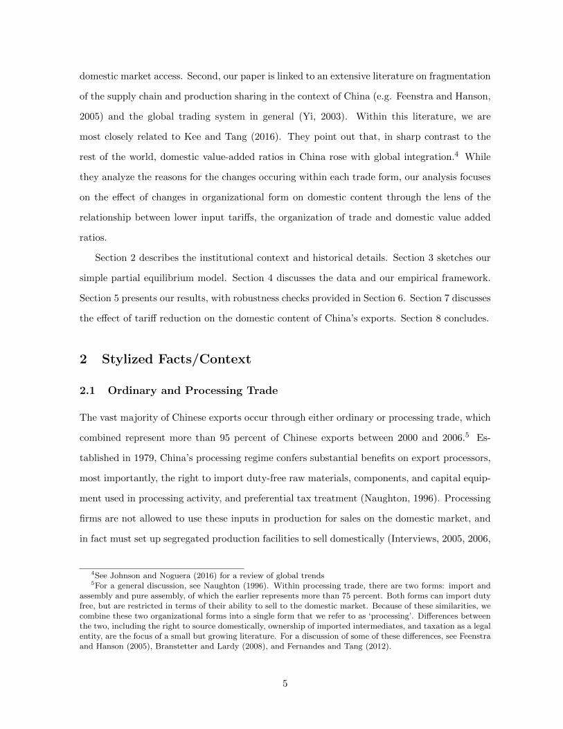
exports organized through ordinary trade in HS industries in 2000 and 2006. Figure 2 shows

the distribution of changes at the HS level between 2000 and 2006. The bottom panel of

Figure 2 drops industries that in 2000 were already completely organized through ordinary

trade. The large mass in the distribution to the right of the origin reflects the general shift

6Segregated facilities helped to reduce the ‘leakage’ of tariff-free intermediates into the local economy.

6

Figure 2: Change in the Share of Ordinary Trade (2000-2006)

0.0

5.1

.15

.2.2

5Fr

actio

n

-1 -.5 0 .5 1Change in the share of exports organized as ordinary: 2000-2006

0.0

5.1

.15

Frac

tion

-1 -.5 0 .5 1Excluding industries completely organized through ordinary in 2000

towards ordinary trade over this period.

A majority of firms–73 percent in 2003–export through a single organizational form. At the

six-digit HS product level, 94.8 percent of all firms in 2003 did the same. Consequently, while

exporting through multiple organizational forms is more common at the firm level, only a small

percentage of firms export a given product through multiple forms.7 Over time, the prevalence

of firms that export a given product through multiple forms also fell from 7.6 percent of all

firms in 2000 to 5.2 percent in 2003, and 3.2 percent in 2006. Consequently, in our theoretical

and empirical framework, we assume that each plant chooses a single form of trade for each

product. Throughout this paper references to ‘sector’ or ‘industry’ are to 1996 HS six-digit

codes unless otherwise indicated.

2.2 Tariffs

In China, tariffs began to come down in the early 1990s as part of a broad set of external reforms

culminating in WTO accession. Statutory tariffs fell from an average of 43.2 percent in 1992

7We also observe that exports by firms exporting through multiple forms accounted for 68.8% of total exportsin 2003. However, exports by firms exporting a given product through multiple organizational forms accountedfor only 33.2 percent of total exports.

7

to 15.1 percent in 2001 and to 9.9 percent in 2007. This was accompanied by an equally sharp

reduction in the dispersion in tariffs (Brandt et al., 2016). Viewed from the perspective of this

fifteen-year period, these cuts and the compression in tariffs reflect policymakers’ objective of

lower and more uniform tariffs. Tariff cuts occurring after 2001 were negotiated in the late

1990s as part of China’s WTO accession.8 Once these tariff cuts were negotiated, they were

locked in, severing the link between tariff cuts and contemporaneous economic changes. As

a result, concerns about possibly endogenous behavior of tariffs are based on expectations of

their effects rather than the effects themselves.

To address concerns about the possible endogeneity of tariff liberalization and lacking a

solid IV strategy, we use long-differences to eliminate time-invariant industry-province factors.

The robustness section also evaluates numerous threats to the exogeneity of tariff cuts including

the initial structure of tariffs across industries, pre-existing trends in input tariffs and ordinary

trade shares, as well as changes in other key variables.

2.3 Domestic Absorption

We define domestic absorption to be the value of total sales of firms manufacturing in China

less exports plus imports. This is our measure of domestic market size. Although China is

often viewed as an ‘export-driven’ economy, exports represent approximately 15 percent of

gross manufacturing output, and domestic absorption exceeds exports in most industries. At

the four-digit China Industrial Classification (CIC) level, domestic absorption for the median

industry in 2004 was 8 times larger than exports, and was greater than exports in 87 percent

of all industries. Over the period we examine, 2000-2006, external demand grew more rapidly

than domestic absorption.

3 Theory

In this section, we sketch a simple partial equilibrium model in which entrepreneurs choose

between organizing production into either ordinary or processing trade.9 Input tariffs and

8Brandt et al. (2016) discuss the institutional context of this round of tariff liberalization in detail.9We purposefully do not explore the full general equilibrium of the model. This requires a model that

captures how falling tariffs affect both global sourcing decisions and product and factor market competition,

8

domestic demand affect the distribution of exports within an industry between ordinary and

processing. The key trade-off that we highlight is that exporting through ordinary trade allows

a product to be sold on the domestic market but at the cost that the firm incurs tariffs on

imported intermediate inputs. Processing trade offers duty-free import of intermediate inputs

but prohibits sale of the product on the domestic market.

3.1 Demand

There are two markets: China and the World. Consumers in each market possess identical and

homothetic Cobb-Douglas preferences over an exogenously fixed number of industries indexed i.

Within an industry, monopolistically competitive entrepreneurs each sell a single differentiated

variety that can either be an ordinary or a processing good. We assume that the elasticity of

substitution is the same across all varieties within an industry and equal to σ > 1.10

Entrepreneurs producing the ordinary good can sell it exclusively in the domestic (China)

market (D) or to both domestic and overseas consumers (O). Entrepreneurs producing the

processing good are legally prohibited from selling it domestically and can only sell it to world

consumers (P ). We refer to the choice of which good to produce and the market in which

to sell it (D, O, or P ) as the ‘organization of production’ and the choice of ordinary versus

processing exports as the ‘organization of trade.’

The price an entrepreneur receives for a good produced under organizational form j, (pji ),

depends on their exogenous capability, (φf ). Industry-specific demand shifters for domestic

and World consumers are captured by DCi and DW

i , respectively.11 Thus, revenue demand

functions from selling domestically (D), selling domestically and exporting through ordinary

trade (O), and only exporting through processing (P ), respectively, are given by:

rDi (φf ) =(DCi

) [pDi (φf )

]1−σ, rOi (φf ) =

(DWi +DC

i

) [pOi (φf )

]1−σ, rPi (φf ) = DW

i

[pPi (φf )

]1−σ.

which is beyond the scope of this paper.10We relax these assumptions in the online appendix and consider cases in which: 1. a single entrepreneur

can produce both ordinary and processing goods within an industry; and 2. substitution possibilities betweenvarieties within a single trade form are greater than between ordinary and processing varieties within the sameindustry.

11Specifically DWi = (tiσ/(σ− 1))1−σνi

(PWi

)σ−1YW where ti is any exogenous transport cost for exports to

the World, νi is the share of world income spent in industry i, PWi is the world CES price index for industry iand YW is world income. A domestic analog holds for DC

i .

9

3.2 Inputs, Technology, and Costs

We assume a two-tier production function. In the top tier, there are two factors that are

combined via a Cobb-Douglas technology: labor L (with cost share α) and intermediate inputs

M , (with a cost share 1 − α).12 Labor is paid a factor return w. In the lower tier, imported

intermediate inputs MM , and domestically supplied intermediate inputs MD are combined

into the composite M via a CES technology with an elasticity of substitution ψ.13 Imported

intermediates face an ad-valorem tariff set at the industry level τi unless used in the production

of processing exports. For this section, we assume that input prices (which include transport

costs), pM and pD, are exogenous. We discuss issues associated with pass-through of input

tariff cuts into import prices (pM ) and into prices charged by domestic firms (pD) below. In

addition, firms face a fixed cost of production f ji that we allow to differ by organizational form

and industry.

As suggested by KWW (2012) and KT (2016), the use of imported intermediate inputs

can differ across industries and also across organizational forms within an industry. Assuming

that variable and fixed costs have the same relative factor mix within an organizational form,

total cost functions associated with the three organizational forms are given by:

TCDi ≡ cDi[qfφf

+ fDi

], TCOi ≡ cOi

[qfφf

+ fOi

], TCPi ≡ cPi

[qfφf

+ fPi

],

where qf is output and

cOi = cDi ≡ wα[p1−ψD + γOi (τipM )1−ψ

] 1−α1−ψ

cPi ≡ wα[p1−ψD + γPi (pM )1−ψ

] 1−α1−ψ

. (1)

The total cost functions for domestic and ordinary trade firms (TCDi and TCOi ) are similar in

that both include tariffs τi on their imported intermediate inputs; reflecting the preferential

policies extended to processing activity, the total cost function for processing firms (TCPi ) does

not. If the unit input requirement of imported intermediate inputs is higher for processing than

for ordinary (for reasons unrelated to input tariffs) then γPi > γOi .14 Lemma 1 formalizes the

12In the empirical section, we allow for multiple primary inputs to enter into industries with different inten-sities. Their inclusion at this point does not illuminate the results that follow.

13KT (2016) find ψ to be greater than one in large cross-section of Chinese industries during this period.14Formally, this is seen by using Shephard’s lemma and setting τi = 1.

10

notion that, other things equal, the input bundles associated with production for the domestic

market and ordinary trade are more expensive in industries in which input tariffs are higher.

Lemma 1. For a given pM/pD, both cDi /cPi and cOi /c

Pi are increasing in τi, other things equal.

Proof. Simple inspection of the equations in (1) deliver the result.

Profit functions for domestic, ordinary, and processing organization are as follows:

πDi =DCi

σ

(cDi)1−σ

φσ−1f − cDi fDi , (2)

πOi =DCi +DW

i

σ

(cOi)1−σ

φσ−1f − cOi fOi , (3)

πPi =DWi

σ

(cPi)1−σ

φσ−1f − cPi fPi . (4)

Following the literature, we assume that the fixed cost of production for domestic sales is

smaller than for exporting through either form (e.g. Bernard, Jensen, Redding, and Schott,

2007).

3.3 Sorting

Taking capabilities as given, entrepreneurs in industry i choose the organization of production

that maximizes profit and earn vi (φf ) ≡ max{

0, πDi (φf ), πOi (φf ), πPi (φf )}

.15 Conditional on

exporting, entrepreneurs sort into either ordinary or processing trade depending on whether

πOi (φf ) ≶ πPi (φf ).

We refer to the case in which there are strictly positive amounts of both ordinary and

processing exports in an industry as a ‘diversified equilibrium.’ All exporters for whom

πOi (φf ) > πPi (φf ) > 0 sort into ordinary trade, and all for whom πPi (φf ) > πOi (φf ) > 0

sort into processing. Any exporter for whom πOi (φf ) = πPi (φf ) > 0 is indifferent between or-

ganizational forms. Setting equation (3) equal to (4), the capability of this marginal exporter

is equal to: (φPf)σ−1 ≡

σ[cPi f

Pi − cOi fOi

]DWi

(cPi)1−σ − (DW

i +DCi

) (cOi)(1−σ)

. (5)

15The first argument allows for costless exit.

11

This expression will be strictly positive as long as the two inequalities below are of the same

direction: (cOicPi

)σ−1

≶ 1 +DCi

DWi

andcPi f

Pi

cOi fOi

≶ 1. (6)

When both inequalities are strictly greater than (>), the marginal profit with respect to

capability and the fixed cost of exporting are greater for processing than for ordinary exports.

If they are both strictly less than (<), then the marginal profit with respect to capability and

the fixed cost of exporting are greater for ordinary trade than for processing.16 The first case

describes a setting in which the benefits of importing capital and intermediate inputs duty

free compensate only the most capable entrepreneurs for the higher fixed costs of processing

and the loss of access to domestic consumers. In the second case, only for the most capable

entrepreneurs do the returns to accessing the domestic market compensate for the higher fixed

cost of ordinary exports and loss of duty free intermediate inputs.17

If πOi (φf ) > πPi (φf ) for all active exporters, then a ‘specialized equilibrium’ holds in which

all exporters sort into ordinary exports. Under the opposite inequality, only processing is

chosen for active exporters.18 A specialized equilibrium with only ordinary trade will hold if

ordinary trade is both high marginal profit and low fixed cost such that the first inequality of

(6) is < and the second is >. This can emerge if domestic market size is relatively large and/or

input tariffs are relatively low.19 A specialized equilibrium with only processing trade can

emerge if the profit return to capability is higher for processing and the fixed cost is lower.20

Figure 3 presents a diversified equilibrium in which there is both a larger return to capability

and greater fixed cost for processing. Consistent with this, the processing profit function cuts

the ordinary profit function from below.(φP,1

)σ−1represents the capability at which an

entrepreneur is indifferent between ordinary and processing.(φO,1

)σ−1is the capability at

16Both of these cases can be seen easily by examining the profit functions associated with each organizationalform of production: equations (3) and (4).

17If there are no differences in fixed costs, all exporters choose the organizational form with greater marginalprofit.

18As in Melitz (2003), this requires that some firms choose to export.19Technically, it can also hold if the inequalities in (6) are both < but the profits of the marginal firm are

negative.20This is the case when firms produce for the domestic market and export through processing alone. In

practice, these types of firms are rare: only 1.4% of firms produce for the domestic market and export throughprocessing but not ordinary trade.

12

Figure 3: Higher Marginal Return to Processing Exports

π φσ−1( )

π D φσ−1( )

π O φσ−1( )π P φσ−1( )

φ*( )σ−1

φO,1( )σ−1

φ P,1( )σ−1

φσ−1− fiDci

D

− fiPci

P

− fiOci

O

which entrepreneurs are indifferent between selling exclusively to the domestic economy and

exporting through ordinary trade. Entrepreneurs with capability φf < φ∗ exit. The solid

line depicts vi (φ). In this case, the least capable entrepreneurs exit, the low intermediate

capability entrepreneurs produce only for the domestic market, high intermediate capability

entrepreneurs organize through ordinary trade, and the most capable entrepreneurs organize

through processing.

Figure 4 presents a diversified equilibrium in which ordinary trade offers a higher return to

capability, but at a greater fixed cost.(φP,2

)σ−1denotes the level of capability for which an

entrepreneur is indifferent between domestic sales and processing trade, and(φO,2

)σ−1is the

critical cut-off between export processing and ordinary trade. φ∗ is unchanged between the two

figures. In the second case, the least capable entrepreneurs exit, low intermediate capability

entrepreneurs produce only for the domestic market, high intermediate capability entrepreneurs

organize through processing, and the most capable entrepreneurs organize through ordinary

trade.

We remain agnostic as to which ordering of the inequalities is most likely to hold at the

industry level. As we show below, in both cases the key finding holds, namely, that relative

trade shares respond to changes in input tariffs and differences in the size of the domestic

13

Figure 4: Higher Marginal Return to Ordinary Exports

π φσ−1( )

π D φσ−1( )

π O φσ−1( )π P φσ−1( )

φ*( )σ−1

φ P,2( )σ−1

φO,2( )σ−1

φσ−1− fi

DciD

− fiPci

P

− fiOci

O

relative to the foreign market across industries.21 Either ordering can be rationalized, and

is model-dependent.22 For example, if R&D causes substantial fixed costs in processing or

if intermediate input tariffs are high, then Figure 3 is empirically relevant. Alternatively, if

capital investment or identifying export markets causes high fixed costs for ordinary trade, and

if a high premium is also placed on the ability to access the domestic market, then Figure 4

should hold.

3.4 Specialized Equilibrium: Comparative Statics

If πPi (φf ) > πOi (φf ) for all firms that choose to export, then all exporters organize through

processing. Lower input tariffs can cause some firms to switch to ordinary trade, leading to a

diversified equilibria as in Figure 3 or 4. This increases the share of ordinary exports from zero

to some positive amount.23 An increase in the size of the domestic market relative to foreign

can have a similar effect. If πOi (φf ) > πPi (φf ) for all exporters, then all exporters organize

through ordinary trade, and lower input tariffs and/or a larger relative domestic market size

21All results continue to go through if selling domestically is high fixed cost/high marginal profit relative toprocessing as well.

22Recent research arguing that processing firms are less productive than firms engaged in ordinary tradesuggests the ordering in Figure 4. See Yu (2015) and Manova and Yu (2016).

23If the change in input tariffs is large enough, the industry can shift from being completely organized throughprocessing to being completely organized through ordinary trade.

14

cannot increase the share of ordinary exports any more. However, the level of ordinary exports

will increase in this case. For this reason, the empirical section also examines the effect of falling

input tariffs and relative market size on export levels.24

3.5 Diversified Equilibrium: Comparative Statics

To develop crisp predictions for the share of ordinary trade when ordinary and processing

co-exist in an industry, we assume that productivity follows a Pareto distribution, with φmin,i

representing the minimum productivity draw in industry i, and k > σ − 1 the common shape

parameter.25 We define the (value) share of total exports that occur through ordinary trade

in industry i as SO,i ≡VO,i

VO,i+VP,iwhere Vj,i is the value of shipments in industry i through

organizational form j. Proposition 1 lays out the relevant comparative static results for changes

in input tariffs and relative market size (holding the other constant):

Proposition 1. Suppose that 0 < SO,i < 1. If τi falls, holdingDCiDWi

fixed, then SO,i rises

regardless of which organizational form is high return to capability/high fixed cost. IfDCiDWi

rises, holding τi fixed, then SO,i rises regardless of which organization of exporting is highreturn to capability/high fixed cost.

Proof. See the online appendix.

For the sorting depicted in Figure 3, lower input tariffs increase the marginal profit to

ordinary exporting as marginal costs fall and profits rise for entrepreneurs that previously were

not able to overcome the fixed cost of ordinary exports. Consequently, some entrepreneurs that

previously only sold domestically now export the ordinary good as the minimum capability

necessary for ordinary trade also falls[(φO,1

)σ−1 ↓]. In addition, some entrepreneurs that

previously chose to organize through processing trade now switch into ordinary trade due to

a falling cost advantage of processing trade. As a result, the minimum capability at which

entrepreneurs organize through processing trade rises[(φP,1

)σ−1 ↑]. On the intensive margin,

falling input tariffs lower input prices which are passed through into lower prices, causing

export levels of incumbent ordinary exporters to rise while there is no change for processing

24The online appendix presents graphically the comparative statics discussed in this subsection.25This restriction ensures industry revenue is finite.

15

exporters who are not subject to these tariffs. Consequently, the share of exports organized

through ordinary trade increases on both the extensive and intensive margins.

For the sorting in Figure 4, lower input tariffs increase both the marginal return to exporting

through ordinary trade and of selling domestically as marginal costs fall for entrepreneurs

organizing through those two forms of production. Consequently, some entrepreneurs that

previously chose to organize through processing trade now switch into ordinary trade due to a

falling cost advantage of processing trade[(φO,2

)σ−1 ↓]

and some entrepreneurs that previously

exported through processing choose to sell only on the domestic market[(φP,2

)σ−1 ↑]. Again,

the level of ordinary exports increases for incumbent ordinary exporters due to lower input

prices. Consequently, the share of exports organized through ordinary trade increases on

both the extensive and intensive margins. In both cases, a larger domestic market relative to

international demand also increases the attractiveness of organizing through ordinary trade,

leading to an increase in the share of exports organized through ordinary trade.

3.6 Pass-Through

Our theoretical framework assumes that pD and pM are both exogenous and do not respond to

changes in tariffs. This implies 100% pass-through of lower tariffs into the price that firms pay

for imported inputs (1 + τ)pM and 0% pass-through into the price of domestically provided

inputs pD. We now briefly discuss departures from this assumption and discuss evidence

regarding pass-through in China during this period.

Consider the case of complete pass-through of lower input tariffs into the price that firms

pay for domestically provided inputs such that a one percent fall in input tariffs also causes

pD also to fall by one percent. If pM is exogenous and fixed, the relative price of domestically

provided inputs to foreign-provided inputs (pD/ ((1 + τ)pM )) does not change and firms that

are subject to tariffs do not substitute between domestically provided and imported interme-

diates occurs. Ordinary firms’ sales expand as the prices of each of their intermediate inputs

fall because they benefit from both lower tariffs on imported goods and lower prices for do-

mestically provided inputs. Average cost for firms engaged in processing trade also falls even

though they do not pay tariffs on imported inputs. This is because the price of domestically

16

provided inputs falls.26 Average cost for processing declines by less than for ordinary exporters

because they do not benefit from lower input tariffs on imported inputs. While total industry

ordinary exports increase due to lower average costs, the change in total processing exports is

ambiguous as some firms might reorganize into ordinary trade. The share of ordinary trade

increases.

Pass-through into the prices of domestically provided inputs has been shown to be strong

in China. Brandt et al. (2016) find that the pass-through of tariff cuts into the price of

domestically provided intermediates is approximately 0.4 over a one-year window. Long-run

pass-through is likely even larger. For import prices, Han et al. (2016) also find evidence of

incomplete pass-through. They estimate that a one percent lower tariff results in an approxi-

mately 0.5 percent lower (tariff inclusive) price of imported goods.27 The similarity in the two

estimates suggests that the relative price of inputs from these two sources changes very little

with tariff cuts, thereby mitigating any possible substitution effects between them.

4 Data

We use trade transaction data collected by the Customs Administration of China available

for the years 2000-2006. These data provide firm-level information at the 8-digit HS level

on the quantity and value of exports and imports, destination and source countries, whether

goods are exported directly or through Hong Kong, organizational form (e.g. processing and

ordinary trade), and ownership type (e.g. foreign- or Chinese-owned). To link data over time,

we aggregate these data to the six-digit HS level.28 We use the full sample of transactions data

rather than the commonly used matched transactions-manufacturing sample [as in KT (2016)

and Manova and Yu (2016)] because the latter omits small firms who tend to organize through

ordinary trade.

A key variable of interest in our analysis is input tariffs. Generally speaking, a firm’s

26Processing firms do use domestically provided inputs. KT (2016) and KWW (2012) estimate that thedomestic value added ratio for processing exports is between 0.4 and 0.5. Pass-through of lower tariffs intothe price of domestically provided inputs can also cause substitution toward these inputs by processing firmsconsistent with the evidence presented in KT (2016).

27Han et al. (2016) Table 2, column 1.28A change in HS codes in 2002 requires us to use a concordance linking pre- and post-2002 codes.

17

Figure 5: Input Tariffs (τI,it): 2000 & 2006

0.1

.2.3

Frac

tion

0 5 10 15 20 25 30Input tariff (2000)

0.1

.2.3

.4.5

Frac

tion

0 5 10 15 20 25 30Input tariff (2006)

input tariff is a weighted average of tariffs applied to goods imported by the firm. Following

the literature (e.g. Brandt et al., 2016), we use input tariffs that are constructed by passing

statutory tariffs through the Chinese input-output matrix.29 The resulting tariffs therefore

vary at the Chinese Input-Output (IO) classification level.30 By construction, all variation in

input tariffs over time comes from changes in the statutory tariffs and not from changes in

the intensity with which these inputs are used. Figure 5 presents histograms of the calculated

input tariffs in 2000 and 2006. We observe a clear fall and compression in input tariffs with

the average input tariff calculated at the IO industry level falling from 11.43 percent to 6.49

percent between 2000 and 2006.

Domestic absorption for industry i, DDit , is total industry sales in the domestic (Chinese)

market. By definition, it is equal to the sum of total sales of all firms in that industry producing

in China minus exports plus imports. The manufacturing census data that are required to

calculate this variable are only available for 1995, 2004, and 2008 at the Chinese Industrial

Classification (CIC) level.31 We interpolate to obtain annual values for 2000-2003 and 2005-

2006. Appendix A describes this in detail. As required by theory, we divide domestic absorption

29We use the 2004 input-output matrix.30There are 84 of these codes.31There are 352 of these codes, each of which maps into approximately 6-8 HS codes.

18

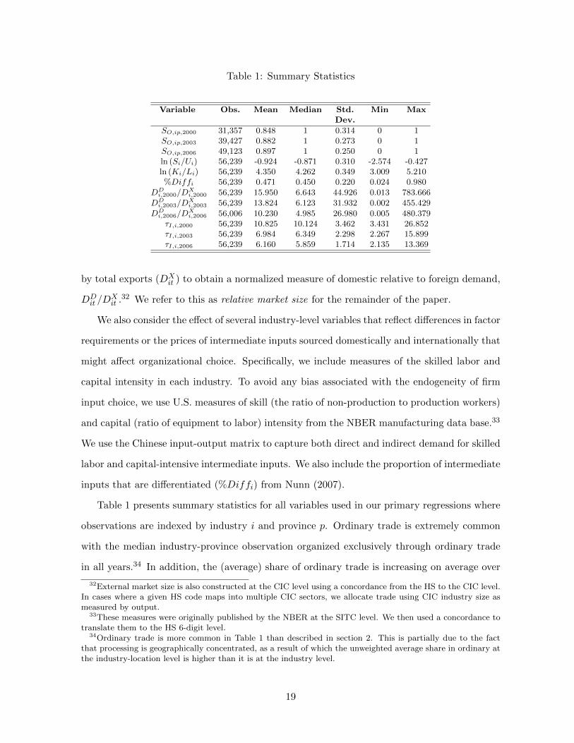
Table 1: Summary Statistics

Variable Obs. Mean Median Std. Min MaxDev.

SO,ip,2000 31,357 0.848 1 0.314 0 1SO,ip,2003 39,427 0.882 1 0.273 0 1SO,ip,2006 49,123 0.897 1 0.250 0 1ln (Si/Ui) 56,239 -0.924 -0.871 0.310 -2.574 -0.427ln (Ki/Li) 56,239 4.350 4.262 0.349 3.009 5.210%Diffi 56,239 0.471 0.450 0.220 0.024 0.980

DDi,2000/D

Xi,2000 56,239 15.950 6.643 44.926 0.013 783.666

DDi,2003/D

Xi,2003 56,239 13.824 6.123 31.932 0.002 455.429

DDi,2006/D

Xi,2006 56,006 10.230 4.985 26.980 0.005 480.379

τI,i,2000 56,239 10.825 10.124 3.462 3.431 26.852τI,i,2003 56,239 6.984 6.349 2.298 2.267 15.899τI,i,2006 56,239 6.160 5.859 1.714 2.135 13.369

by total exports (DXit ) to obtain a normalized measure of domestic relative to foreign demand,

DDit /D

Xit .32 We refer to this as relative market size for the remainder of the paper.

We also consider the effect of several industry-level variables that reflect differences in factor

requirements or the prices of intermediate inputs sourced domestically and internationally that

might affect organizational choice. Specifically, we include measures of the skilled labor and

capital intensity in each industry. To avoid any bias associated with the endogeneity of firm

input choice, we use U.S. measures of skill (the ratio of non-production to production workers)

and capital (ratio of equipment to labor) intensity from the NBER manufacturing data base.33

We use the Chinese input-output matrix to capture both direct and indirect demand for skilled

labor and capital-intensive intermediate inputs. We also include the proportion of intermediate

inputs that are differentiated (%Diffi) from Nunn (2007).

Table 1 presents summary statistics for all variables used in our primary regressions where

observations are indexed by industry i and province p. Ordinary trade is extremely common

with the median industry-province observation organized exclusively through ordinary trade

in all years.34 In addition, the (average) share of ordinary trade is increasing on average over

32External market size is also constructed at the CIC level using a concordance from the HS to the CIC level.In cases where a given HS code maps into multiple CIC sectors, we allocate trade using CIC industry size asmeasured by output.

33These measures were originally published by the NBER at the SITC level. We then used a concordance totranslate them to the HS 6-digit level.

34Ordinary trade is more common in Table 1 than described in section 2. This is partially due to the factthat processing is geographically concentrated, as a result of which the unweighted average share in ordinary atthe industry-location level is higher than it is at the industry level.

19

time.35 As illustrated in Figure 5, input tariffs fell by an average of 4.7 percentage points.

Although the domestic market was larger than exports in each year, it grew less rapidly; as a

result, relative domestic market size declined over time.

4.1 Estimation Details

Our primary outcome of interest is the value share of exports organized through ordinary trade:

SO,ipt ≡VO,ipt

VO,ipt + VP,ipt, (7)

where VO,ipt and VP,ipt are export values organized through ordinary and processing trade,

respectively, for industry i in province p in year t. We examine the organization of trade at

this level for four reasons. First, in contrast to the firm-level, industry-level analysis allows

us to quantify the extensive margin’s contribution to total changes. Second, ordinary trade

firms are generally small. For this reason, average changes in ordinary trade at the firm level

often differ from changes at the industry level. Third, geographic heterogeneity may play an

important role in determining firms’ choice of organizational form (Defever and Riano, 2012).

In the Chinese context, special economic zones are prominent. And fourth, we conduct our

analysis at the six-digit HS level, as opposed to the four-digit CIC, to examine more finely the

product-level extensive margin.

In the cross section, we estimate equation (8) for each of the years t ∈ {2000, 2003, 2006}

ln(SO,ipt) = βI,t ln(τI,it) + β′X,tXit + Φpt + εipt (8)

where τI,it is the input tariff, Xit is a vector of explanatory variables, and Φpt is a province

fixed effect for that cross-section. We use provincial fixed effects to control for factors such

as the presence of special economic zones that might make some geographic locations more

likely to be organized into ordinary or processing trade. Finally, εipt is an error term that is

clustered at the IO-industry level to account for the fact that multiple HS industries may map

into a single IO industry at which the input tariff is defined, and that other control variables

35The number of observations on trade shares is less than that on tariffs and industry characteristics becauseexports in some observations are zero.

20

are only defined at the industry level and not the industry-province level.

In the cross-section, we use Tobit estimators that are censored from above at ln(1) = 0.

We discuss censoring from below in section 6. Our dependent variable is undefined if there

are no exports, and so our panel is unbalanced. Finally, because exporting activity by a

different number of firms underlie each observation, heteroskedasticity might compromise the

consistency of our estimates. For this reason, we weight each observation by the number of

firms in the industry-province cell.

In order to eliminate any time-invariant industry-province effects that might be correlated

with input tariffs, we also estimate the relationship by taking first differences of equation (8)

between 2000 and 2006. Our estimating equation is then given by equation (9):

∆ ln(SO,ipt) = β∆I∆ ln(τI,it) + β′XXi + Φp + ε∆,ipt (9)

where standard errors are clustered at the IO level and variables are defined analogous to

equation (8).36 Input tariff reductions between 2000 and 2006 are defined as negative. The

coefficients β′X now capture differential trends in the share of ordinary exports correlated with

industry observables, and Φp absorbs province-specific trends. Section 6 examines and rules

out reasons why additional industry-specific trends might be correlated with changes in input

tariffs.

5 Results

Columns (1)-(6) of Table 2 present Tobit estimation results of equation (8), while columns

(7) and (8) are linear estimates for equation (9). Columns (7) and (8), which eliminate

time-invariant industry-province factors, are our preferred specifications but we present cross-

sectional results for comparison.

In the individual cross-sections for 2000, 2003 and 2006, the coefficient on input tariffs is

consistently negative and declining slightly. The results suggest that sectors with the lowest

(highest) input tariffs have the highest (lowest) share of ordinary trade. Consistent with our

36Results are robust to two-way clustering at the IO-province level as described by Cameron, Gelbach, andMiller (2008).

21

model, there is also a robust positive correlation in each year between relative market size and

the role of ordinary trade in exports.

The time-series effects of tariffs are similar. Column (8) suggests that a 1 log point cut in

input tariffs increases the average share of ordinary trade by 0.81 log points, ceteris paribus.

With weighting, the average increase in the share of ordinary trade for a given industry-

province pair is 0.54 log points. With input tariffs falling on average by 0.56 log points

[ln(10.83) − ln(6.16)] between 2000 and 2006, this implies that 83% of the average change

in the share of ordinary trade is consistent with falling input tariffs.37 The effect of relative

market size is positive and significant as suggested by theory, and only slightly smaller than in

the cross-section. Table 1 shows that the ratio of domestic absorption to external market size

was actually falling during this period, which partially offset the effect of falling input tariffs

on trade form.

5.1 Levels

Table 3 explores the growth rates of export levels that underlie our results for shares. We do this

for two reasons. First, our model predicts that the level of ordinary trade within an industry-

province pair should rise as input tariffs fall. If there is no pass-through, we might expect

processing exports to decline due to reorganization, although some degree of pass-through

into the price of domestically provided intermediate inputs might provide a countervailing

force as discussed in section 3.6. Second, the large number of observations that are organized

exclusively through ordinary trade precludes an increase in the share of ordinary trade but

does allow for increased levels in response to lower input tariffs.

We start by estimating the following regression where ∆ ln(Vipt) is the log change in export

value between 2000 and 2006 in the industry-province pair ip:

37This large contribution is not due to our weighting scheme. The unweighted average change is 0.10 logpoints. The weighted average of 0.54 log points reflects the fact that industry-province pairs with more firmsincreased their share of ordinary trade more than those with fewer firms. Estimating equation (9) withoutweights delivers a coefficient on input tariffs of 0.24 [p = 0.07] suggesting an even larger contribution of fallingtariffs to the increase in the ordinary share of trade (1.35=0.24*0.56/0.10) suggesting mitigating effects fromother factors. The change in relative market size can be one such mitigating factor.

22

Table 2: Baseline Estimation

Dep. Var: Dep. Var:ln

(SO,ipt

)∆ ln

(SO,ipt

)2000 2000 2003 2003 2006 2006 2000-2006(1) (2) (3) (4) (5) (6) (7) (8)

ln(τI,it

)-1.67∗∗∗ -1.01∗∗ -0.82∗∗∗ -0.63∗∗ -0.49∗∗ -0.53∗∗

(0.53) (0.45) (0.32) (0.30) (0.25) (0.23)∆ ln

(τI,it

)-0.90∗∗∗ -0.81∗∗

(0.26) (0.31)ln

(DDit /D

Xit

)0.22∗∗ 0.18∗∗ 0.11∗

(0.10) (0.09) (0.06)∆ ln

(DDit /D

Xit

)0.068∗∗

(0.03)%Diffi -1.33∗∗ -1.36∗∗∗ -1.02∗∗∗ -0.14

(0.62) (0.51) (0.36) (0.12)ln (Si/Ui) -0.55 -0.63 -0.72∗∗∗ 0.029

(0.59) (0.39) (0.26) (0.15)ln (Ki/Li) 0.18 0.043 0.14 -0.076

(0.69) (0.48) (0.30) (0.15)Obs. 30,434 30,434 38,927 38,927 47,406 47,199 26,927 26,839Non-Cens. 7,613 7,613 9,303 9,303 11,468 11,442 . .R-Cens. 22,821 22,821 29,624 29,624 35,938 35,757 . .

Columns (1)-(6) are one-sided Tobits with an (upper) censoring value of ln(1) = 0. Columns (7)and (8) are WLS. Dependent variables are at the top of each column. Standard errors inparentheses are clustered at the IO level. All regressions include province fixed effects. p < 0.01 :∗∗∗, 0.01. ≤ p < 0.05 :∗∗, 0.05 ≤ p < 0.10 :∗. Regressions weighted by the number of firms foreach ip observation.

Table 3: Growth of Total, Ordinary, and Processing Exports

Dep. Var. Dep. Var.∆ ln(Vj,ipt) %∆Vj,ipt

Total Ord. Proc. Total Ord. Proc.(1) (2) (3) (4) (5) (6)

∆ ln(τI,it

)-0.11 -0.91∗ 0.13 -0.075 -0.34∗∗ 0.057(0.27) (0.50) (0.28) (0.13) (0.16) (0.18)

∆ ln(DXit

)1.13∗∗∗ 0.93∗∗∗ 0.90∗∗∗ 0.54∗∗∗ 0.28∗∗∗ 0.62∗∗∗

(0.07) (0.09) (0.05) (0.05) (0.04) (0.04)∆ ln

(DDit /D

Xit

)-0.038 -0.061 -0.078 0.030 -0.0057 -0.0069(0.03) (0.05) (0.06) (0.02) (0.02) (0.03)

%Diffi -0.20∗ -0.29 0.083 -0.023 -0.014 -0.11(0.12) (0.21) (0.28) (0.06) (0.07) (0.20)

ln (Si/Ui) 0.14 0.16 0.76∗∗∗ 0.0053 0.014 0.40∗∗∗

(0.09) (0.20) (0.15) (0.05) (0.07) (0.11)ln (Ki/Li) 0.020 0.040 -0.13 0.020 0.076 -0.11

(0.07) (0.15) (0.12) (0.04) (0.07) (0.07)Obs. 27,655 26,839 6,483 47,436 47,079 11,666Non-Cens. . . . 27,655 26,839 6,483R-Cens. . . . 19,781 20,240 5,183

Columns (1)-(3) are WLS and columns (4)-(6) are two-sided Tobits withcensoring values of -2 and 2. Dependent variables given at the top of eachcolumn. Standard errors in parentheses are clustered at the IO level. Allregressions include province fixed effects. p < 0.01 :∗∗∗, 0.01 ≤ p < 0.05:∗∗, 0.05 ≤ p < 0.10 :∗. Regressions weighted by the number of firms foreach ip observation.

23

∆ ln(Vipt) = β∆I∆ ln(τI,it) + β′XXi + Φp + ε∆′,ipt. (10)

We then run similar regressions where the dependent variables are ordinary exports and pro-

cessing exports, ∆ ln(VO,ipt) and ∆ ln(VP,ipt), respectively. One difference between this esti-

mating equation and the one for shares [equation (9)] is the need to control for changes in

total demand at the industry level that are differenced out when looking at shares. To do

this we follow an IV strategy in which we include the increase in Chinese exports to the world

[∆ ln(DXit

)] and then instrument for it using the change in world trade (excluding China).38

Columns (1)-(3) of Table 3 present these results.

We also estimate these relationships using as the dependent variable a proportional change

calculated from a midpoint average:

%∆Vipt =Vip,2006 − Vip,2000

0.5 ∗ [Vip,2006 + Vip,2000]

that is bound between [-2,2] by design and is estimated using a two-sided Tobit with censoring

at these values.39 This transformation has the advantage of accommodating values of zero in

2000 or 2006 (but not both) and is common in the job creation and destruction literature [see

Levinsohn (1999) and Haltiwanger, Jarmin, and Mir (2013)]. These results appear in columns

(4)-(6). Columns (1) and (4) show no statistically significant relationship between changes in

input tariffs and total exports although the point estimate is negative. As expected however,

falling input tariffs increase ordinary exports [columns (2) and (5)]. The effects on processing

exports [columns (3) and (6)] are not significantly different from zero.

5.2 Imports and Heterogeneous Effects

Our theory suggests that falling input tariffs should also increase the share of imports organized

through ordinary trade. We examine this relationship in Table 4, where the dependent variable

is the (log) share of imports organized through ordinary trade, ln(SMO,ipt). For comparability,

we use the output tariff calculated at the same level as the input tariff that we use in Table 2.

38This is calculated at the HS six-digit level. The instrument is strong well above conventional levels.39Dependent variables for ordinary and processing in columns (5) and (6) are defined analogously.

24

The relationship between lower output tariffs and the change in the share of imports coming

through ordinary trade [column (8)] is positive, but only marginally significant [p = 0.12].

To explore this result further, Table 5 examines whether there are heterogeneous effects of

lower input tariffs by type of good. Using the United Nations Broad Economic Classification

(BEC) system, we classify goods into three basic categories: consumption goods, capital goods,

and intermediate inputs. In our regressions, we include a set of interactions terms involving

indicators for these categories and our tariff measures. The omitted category in all regressions

is consumption goods. Because processing trade most prominently involves the imports of

intermediate inputs and capital goods for further assembly and re-export, we expect our results

to be strongest for these two types of goods and do not expect them to hold for imports of

final consumption goods. Since processing trade involves the use of imported intermediates in

the manufacture and exporting of all types of goods, we have no strong prior about how our

results might differ by the type of exported good.

Columns (1) and (4) of Table 5 replicate column (8) of Tables 2 and 4, respectively. Columns

(2) and (5) add indicator variables for capital goods and intermediate inputs, BECK,i and

BECINT,i. Columns (3) and (6) include the interaction terms. Column (3) is consistent with

our prior that the effect of lower input tariffs does not depend on the type of good that is being

produced for export. Furthermore, column (6) suggests that input tariffs influence the choice

between importing through ordinary or processing in the case of intermediate and capital

goods, but have no effect on consumption goods.

5.3 Decomposition

There are a number of alternative margins through which the increase in ordinary trade may

have occurred. We start by decomposing the total effect into the contributions of domestic

and foreign firms. Both play a prominent role in China’s exports. In 2000, 53% (47%) of

total exports was through foreign (domestic) firms. Of total exports by foreign firms, 13%

was through ordinary trade in 2000, while 59% of total exports by domestic firms was through

ordinary. Our concern here is that other policy changes implemented concurrently with the

25

Table 4: Imports

Dep. Var: Dep. Var:

ln(SMO,ipt

)∆ ln

(SMO,ipt

)2000 2000 2003 2003 2006 2006 2000-2006(1) (2) (3) (4) (5) (6) (7) (8)

ln(τO,it

)-1.50∗ -0.98∗∗ -0.86 0.063 -0.034 0.44(0.77) (0.49) (0.62) (0.49) (0.35) (0.40)

∆ ln(τO,it

)-0.20 -0.35(0.30) (0.22)

ln(DDit /D

Xit

)0.20∗∗ 0.21∗∗ 0.18∗

(0.09) (0.10) (0.10)∆ ln

(DDit /D

Xit

)0.10

(0.09)%Diffi 3.77∗∗∗ 3.25∗∗∗ 2.38∗∗∗ -1.26∗∗∗

(0.99) (0.79) (0.63) (0.37)ln (Si/Ui) 2.53∗∗∗ 1.96∗∗∗ 1.33∗∗ -1.50∗∗∗

(0.65) (0.74) (0.60) (0.35)ln (Ki/Li) 0.48 0.37 0.31 -0.067


Columns (1)-(6) are one-sided Tobits with an (upper) censoring value of ln(1) = 0.Columns (7) and (8) are WLS. Dependent variables are at the top of each column.Standard errors in parentheses are clustered at the IO level. All regressions includeprovince fixed effects. p < 0.01 :∗∗∗, 0.01. ≤ p < 0.05 :∗∗, 0.05 ≤ p < 0.10 :∗.Regressions weighted by the number of firms for each ip observation.

Table 5: Heterogeneous Effects

Panel A: Exports Panel B: ImportsDep. Var: Dep. Var:

∆ ln(SO,ipt) ∆ ln(SMO,ipt)

(1) (2) (3) (4) (5) (6)

∆ ln(τI,it

)-0.81∗∗ -0.83∗∗∗ -1.12∗∗ ∆ ln

(τO,it

)-0.35 -0.33 0.24

(0.31) (0.29) (0.51) (0.22) (0.23) (0.27)BECK,i ∗∆ ln

(τI,it

)-0.26 BECK,i ∗∆ ln

(τO,it

)-0.54∗

(1.27) (0.33)BECINT,i ∗∆ ln

(τI,it

)0.46 BECINT,i ∗∆ ln

(τO,it

)-0.65∗

(0.54) (0.38)∆ ln

(DDit /D

Xit

)0.068∗∗ 0.086∗∗ 0.087∗∗ ∆ ln

(DDit /D

Xit

)0.10 0.091 0.090

(0.03) (0.04) (0.04) (0.09) (0.09) (0.09)BECK,i 0.047 -0.084 BECK,i -0.16 -0.46∗

(0.10) (0.71) (0.19) (0.25)BECINT,i 0.080 0.34 BECINT,i 0.038 -0.32

(0.07) (0.29) (0.17) (0.28)%Diffi -0.14 -0.080 -0.12 %Diffi -1.26∗∗∗ -1.08∗∗∗ -1.10∗∗∗

(0.12) (0.15) (0.17) (0.37) (0.36) (0.36)ln (Si/Ui) 0.029 0.0053 0.018 ln (Si/Ui) -1.50∗∗∗ -1.46∗∗∗ -1.48∗∗∗

(0.15) (0.13) (0.13) (0.35) (0.37) (0.37)ln (Ki/Li) -0.076 -0.073 -0.079 ln (Ki/Li) -0.067 -0.094 -0.086

(0.15) (0.14) (0.14) (0.28) (0.29) (0.29)Obs. 26,839 26,806 26,806 Obs. 22,164 22,164 22,164

All regressions are WLS. Dependent variables given at the top of each column. Standard errors in parenthesesare clustered at the IO level. All regressions include province fixed effects. p < 0.01 :∗∗∗, 0.01 ≤ p < 0.05 :∗∗

, 0.05 ≤ p < 0.10 :∗. Regressions weighted by the number of firms for each ip observation.

26

Table 6: Decomposition

Total Domestic Foreign Domestic Foreign Domestic Foreign Domestic ForeignIncumbent Incumbent New New Exit Exit

%∆SO,ipt DOMO,ipt FORO,ipt DOMIO,ipt FORIO,ipt DOMN

O,ipt FORNO,ipt DOMEO,ipt FOREO,ipt

(1) (2) (3) (4) (5) (6) (7) (8) (9)

∆ ln(τI,it

)-0.61∗∗ -0.45∗ -0.15 -0.075 -0.080 -0.19 -0.12 -0.18∗ 0.040∗

(0.24) (0.23) (0.12) (0.10) (0.05) (0.18) (0.08) (0.10) (0.02)∆ ln

(DDit /D

Xit

)0.056∗∗ 0.051∗∗∗ 0.0053 -0.00072 0.0069 0.011 -0.0097 0.041∗∗∗ 0.0081∗∗

(0.02) (0.02) (0.01) (0.01) (0.01) (0.01) (0.01) (0.01) (0.00)%Diffi -0.053 -0.063 0.013 -0.061 -0.036 -0.091 0.046 0.089 0.0030

(0.10) (0.10) (0.04) (0.04) (0.03) (0.06) (0.04) (0.07) (0.01)ln (Si/Ui) -0.11 -0.17∗∗ 0.064 0.0021 -0.00085 -0.12∗∗∗ 0.064 -0.055 0.0011

(0.12) (0.08) (0.05) (0.04) (0.02) (0.04) (0.04) (0.06) (0.01)ln (Ki/Li) 0.021 0.071 -0.052 -0.041∗ -0.0036 0.053 -0.026 0.059 -0.023∗∗∗

(0.12) (0.08) (0.05) (0.02) (0.02) (0.04) (0.04) (0.05) (0.01)Obs. 27,597 27,597 27,597 27,597 27,597 27,597 27,597 27,597 27,597L-Cens. 95 73 18 1 8 0 0 72 9Non-Cens. 26,839 27,265 27,509 27,589 27,575 27,364 27,550 27,525 27,588R-Cens. 663 259 70 7 14 233 47 0 0

All regressions are two-sided Tobits with censoring values of -2 and 2. Dependent variables given at the top of each column.Standard errors in parentheses are clustered at the IO level. All regressions include province fixed effects. p < 0.01 :∗∗∗,0.01 ≤ p < 0.05 :∗∗, 0.05 ≤ p < 0.10 :∗. Regressions weighted by the number of firms for each ip observation.

tariff cuts might have encouraged greater entry by Chinese-owned firms, in which case the

correlation between tariffs and ordinary trade shares would be spurious. One specific policy

is the universal extension of direct trading rights in 2004 to domestically-owned firms, rights

which foreign-owned firms already possessed (see Bai, Krishna, and Ma, 2015). Second, because

of potential differences between domestic and foreign firms in the use of imported intermedi-

ates within each trade form, the effect of tariffs on their choices may matter for the overall

relationship between tariffs and domestic value added ratios.

Because the change in the log of a sum of components cannot be decomposed exactly, we

use the proportional change in the share of ordinary trade %∆SO,ipt ≡SO,ip,2006−SO,ip,2000

0.5∗[SO,ip,2006+SO,ip,2000] ,

and decompose it into components due to changes in domestic and foreign firms:40

%∆SO,ipt = DOMO,ipt + FORO,ipt.

40Formally, start by defining V DO,ipt as ordinary exports by domestic firms, and Vipt as total exports. Then, we

can define DOMO,ipt ≡V DO,ip,2006Vip,2006

−V DO,ip,2000Vip,2000

0.5∗[SO,ip,2006+SO,ip,2000]as the contribution of domestic firms to the total proportional

increase in the share of ordinary trade. An analogous expression holds for the contribution of foreign firmsFORO,ipt with the sum of the two equaling the total proportional change, %∆SO,ipt. Appendix B describesthis in more detail.

27

Under the properties of linear regression, the marginal effects of lower input tariffs for these

two components sum to the total effect.41 Column (1) of Table 6 presents the effect of lower

input tariffs on the total change in the share of ordinary trade, %∆SO,ipt. Columns (2) and (3)

decompose this into the contributions of domestic and foreign firms, DOMO,ipt and FORO,ipt.

Domestic firms account for the largest share of the total change (75%), highlighting their

importance in the expansion of ordinary trade. The contribution from foreign firms is non-

negligible (25% of the total), however it is not statistically significant. This can be either

because foreign firms were not increasing their share of ordinary trade or their small overall

share of ordinary trade makes their contribution difficult to pick up. If the former, we are

concerned that our results reflect reforms benefitting domestically-owned firms rather than the

effect of input tariffs. Consequently, in Appendix C we examine the percentage increase in the

share of ordinary exports in domestic and foreign firms separately. For both subsamples, we

find large, positive and significant effects of falling input tariffs on the share of ordinary trade.

Thus, while both domestic and foreign firms increased their “within” share of ordinary trade,

the contribution of domestic firms to the total change was much larger.

Next, we further decompose the total effect into components due to incumbents (I), new

firms (N), and exiting firms (E), allowing each of these to be further divided into domestic

and foreign firm components:42

%∆SO,ipt = DOM IO,ipt + FORIO,ipt︸︷︷︸incumbents

+DOMNO,ipt + FORNO,ipt︸︷︷︸new firms

+DOMEO,ipt + FOREO,ipt︸︷︷︸exiting firms

.

Incumbent firms [columns (4) and (5)] are those that sell the same product in 2000 and 2006.

New firms [columns (6) and (7)] are those that start exporting a product between 2000 and

2006.43 Exiting firms [columns (8) and (9)] are those that stop exporting a product between

2000 and 2006. Again, the sum of the marginal effects of the change in tariffs for these

components [columns (4)-(9)] equals the total effect [column (1)].

41Although Tobit is a non-linear estimator, the small number of censored values when looking at proportionalchanges leads it to closely resemble linear regression.

42These terms are derived analogously as in footnote 40. See Appendix B for more details of this decomposi-tion.

43In this group, we include firms that exported another product in 2000 and added the relevant product after2000. These are not quantitatively important.

28

On the intensive margin, we find similar point estimates for both domestic and foreign

incumbent firms. Falling input tariffs also cause the share of ordinary trade to increase due to

entry of new domestic and foreign exporters, with domestic firms playing a slightly stronger

role. Finally, we find that falling input tariffs increased ordinary trade shares due to less exit

by domestic firms but lower ordinary trade due to increased exit by foreign firms, however the

net effect of the two is to increase the share of ordinary trade.

The strong role for new exporters in increasing the share of ordinary trade (columns 6 and

7) is consistent with the ordering in Figure 3 as lower input tariffs allow intermediate capability

firms who had previously only sold domestically to overcome the fixed costs of exporting and

enter into ordinary trade. However, the role for exit (columns 8 and 9) is consistent with

intermediate capability firms leaving processing to sell on the domestic market alone as the

preferential treatment associated with processing trade diminishes.44 Therefore, our results

suggest that the data fall somewhere in between Figure 3 in which processing trade is high

return to capability/high fixed cost relative to ordinary trade and Figure 4 in which the opposite

is true.

6 Robustness

We now examine the robustness of our results to a potential number of concerns including

functional form, the sample of observations we use, and endogeneity issues that pose threats

to our identification strategy.

6.1 Functional Forms

We re-estimate equation (8) using two alternative specifications. Results appear in Appendix

D. With SO,ipt as the dependent variable, we use two-sided Tobits that allow for censoring at

SO,ipt = 0 and SO,ipt = 1. Comparable estimates are provided for equation (9), where the

44Tables 2 and 3 are consistent with either ordering. With no pass-through of lower input tariffs into pricescharged by domestic intermediate input providers, both orderings predict an increase in the level of ordinarytrade and a fall in processing trade as processing exporters sort into ordinary trade. With some pass-throughof lower input tariffs into prices charged by domestic intermediate input providers, the prediction for processingexporters becomes ambiguous as they have access to lower prices charged by domestic providers of intermediateinputs and pass some of these lower prices onto consumers abroad.

29

Table 7: Robustness

No Trading Interior τI,i,2000 Trend ∆τaltI,it China Trend IV Value Finance

Co. in 2000 τI,it Skill SO,ipt Weights

∆ ln(SNTO,ipt) ∆ ln(SO,ipt) ∆ ln(SO,ipt) ∆ ln(SO,ipt) ∆ ln(SO,ipt) ∆ ln(SO,ipt) ∆ ln(S03−06O,ipt ) ∆ ln(SO,ipt) ∆ ln(SO,ipt) ∆ ln(SO,ipt)

(1) (2) (3) (4) (5) (6) (7) (8) (9) (10)

∆ ln(τI,it

)-0.95∗∗ -0.78∗∗ -0.76∗∗∗ -0.77∗∗∗ -0.80∗∗∗ -0.82∗∗ -2.27∗∗∗ -0.78∗∗

(0.39) (0.39) (0.26) (0.28) (0.27) (0.34) (0.79) (0.33)ln

(τI,i,2000

)0.040(0.14)

∆ ln(DDit /D

Xit

)0.080∗ 0.039 0.064∗ 0.065∗∗ 0.10∗∗∗ 0.059 0.051∗∗ 0.059 0.23 0.063∗

(0.04) (0.04) (0.04) (0.03) (0.02) (0.04) (0.02) (0.05) (0.14) (0.04)%Diffi -0.18 -0.43∗∗ -0.15 -0.11 -0.085 -0.11 -0.037 -0.13 -0.044 -0.20

(0.16) (0.16) (0.12) (0.12) (0.12) (0.12) (0.07) (0.12) (0.48) (0.16)ln (Si/Ui) -0.0085 0.26 0.044 0.026 0.019 0.099 0.018 -0.23 0.0097

(0.18) (0.19) (0.15) (0.15) (0.09) (0.08) (0.17) (0.36) (0.14)ln (Ki/Li) -0.14 -0.23 -0.079 -0.058 -0.12 -0.031 -0.028 -0.068 0.28 -0.075

(0.17) (0.16) (0.14) (0.15) (0.09) (0.13) (0.07) (0.17) (0.33) (0.15)

∆ ln(τ96−99I,it

)-0.58

(0.35)

∆ ln(τaltI,it

)-0.44∗∗∗

(0.10)ln(Si/Ui)ch -0.037

(0.09)

∆ ln(τshortI,it

)-0.53∗

(0.28)

∆ ln(S00−02O,ipt

)-0.072∗∗∗

(0.02)exfini -0.16

(0.18)inventi -1.06

(1.45)tangi -0.51

(0.61)RDi 0.51

(0.85)Obs. 17,124 7,471 26,839 26,839 26,709 26,839 23,516 26,839 26,839 26,839

All columns are WLS. Dependent variables are at the top of each column. Standard errors in parentheses are clustered at the IO level except for column (5)in which standard errors are clustered at the HS six-digit level. All regressions include province fixed effects. p < 0.01 :∗∗∗, 0.01 ≤ p < 0.05 :∗∗, 0.05 ≤p < 0.10 :∗. Regressions weighted by the number of firms for each ip observation except column (9) which is weighted the value of exports for each ip observation.

30

dependent variable is the proportional increase in ordinary trade %∆SO,ipt =SO,ip,2006−SO,ip,2000

0.5∗[SO,ip,2006+SO,ip,2000],

which is bound in the interval [-2,2]. Results are robust to this specification. Our results are

also robust to using first differences that are bound in the interval [-1,1].

6.2 Subsamples

Over the period we examine, a significant (29% in 2000), albeit declining portion of China’s

trade was carried out through trading companies. Although we observe both ordinary and

processing exports through trading companies, a potential concern is that for trade interme-

diated by trading companies, the mechanisms outlined in section 3 may be muted by other

factors. Thus, as is common in the literature (e.g. Manova and Yu, 2016), column (1) of Table

7 excludes all firms identified to be trading firms.45 Results are slightly stronger than our

baseline specification.

Column (2) examines a subsample for which there was a strictly positive amount of both

ordinary and processing exports in 2000. This allows us to examine the effect of input tariff

cuts on industry-locations that were not at corners, and had potentially more room for choice

between ordinary and processing. It also drops all province-industry observations that were

already at 100 percent ordinary trade in 2000 and thus could not increase their share of ordinary

trade.

6.3 Additional Tariff Measures

Column (3) includes the initial input tariff level in 2000. This serves two purposes. First, it

controls for pre-WTO levels of protection in an industry. Second, it controls for the possibility

that sectors may have had different trajectories based on their initial tariff level. We are also

concerned that pre-existing trends may be endogenously correlated with our tariff measures,

thus biasing our results. In column (4), we include the change in input tariffs from 1996 to

1999 to help absorb any unobserved heterogeneity.

One common criticism of input tariffs constructed using input-output tables is that they do

not distinguish imported from domestically provided intermediate inputs. By relying on the

45This is done by looking for the Chinese characters for “trading company” in a firm’s name.

31

input tariffs constructed by using the IO matrix, our measures are also rather coarse. Column

(5) uses an input tariff constructed from firm product-level import data in a manner analogous

to Yu (2015).46 Our results are robust to this measure.47

6.4 Additional Endogeneity Concerns

Column (6) considers the possibility that US measures of skill intensity may be inaccurate

measures of the skill requirements of Chinese firms. Consequently, we replace our measure of

skill intensity from the NBER with a measure from the Chinese census. Results are unchanged.

Column (7) examines pre-existing trends in trade shares. Our concern is that pre-existing

trends may be endogenously correlated with our tariff measures, thus biasing our results. We

do not have data on the pre-2000 trends for the share of ordinary trade. However, in column (7),

we run regressions for the change in the share of ordinary trade from 2003 to 2006 using input

tariff cuts over the same period, and include as additional controls the change in ordinary’s

share from 2000 to 2002. Finally, column (8) addresses the fact that domestic absorption

is an endogenously determined outcome because of its normalization by total exports. We

instrument for this using a variable whose denominator contains total world exports (excluding

China) to the world.48 Column (9) weights the observations by total shipments in the industry-

province pair instead of by the number of firms. While the point estimate is much larger, the

qualitative result is unchanged.

Finally, column (10) considers the variables related to financial constraints examined by

Manova and Yu (2016). Specifically, we include: (i) reliance on external financing (exfini); (ii)

the ratio of inventory to sales (inventi) which is commonly thought to reflect liquidity needs,

(iii) the ratio of tangible to total assets (tangi); and (iv) R&D expenditures as a proportion

of total sales (RDi). All variables are from Kroszner et al. (2007). Our results are robust to

their inclusion.49

46The online appendix describes the construction of this alternate input tariff in detail.47While the point estimate is smaller in absolute value, the average change in this measure is larger leading

to similar contributions.48The instrument is strong with a first stage F-statistic of 242 when the data are collapsed to the CIC level.49Although they are insignificant in the results presented here, inventi and tangi are of the expected sign

and are significant in the cross section.

32

7 Implications for Domestic Factor Demand

KWW (2012) and KT (2016) argue that ordinary exports embody a larger share of Chinese

value added than do processing exports. Both papers estimate that the share of domestic value

added in Chinese exports (‘domestic value added ratio’) is 40-50 percentage points higher for

ordinary than processing trade.50 Consequently, our results imply that falling input tariffs

might influence the domestic value added ratio of an industry’s exports by affecting the relative

mix of ordinary and processing trade. However, lower levels of protection might have offsetting

influences that could reduce the share of value paid to domestically provided goods and services.

In particular, reductions in the level of protection that lower the relative price of imported

intermediate inputs might lead firms and industries to substitute away from domestic factors.

In addition, the composition of exports between domestic and foreign firms might also be

altered, inducing changes in overall domestic content depending on differences in domestic

value added ratios between these two types of firms. This section rigorously assesses this

potentially ambiguous effect.

7.1 Calculating Domestic Value Added Ratios

Following KT (2016), we start by calculating the domestic value added ratio (DVAR) for

the exports of each industry. This represents the share of gross export revenue accruing to

domestically provided goods and services. To do so, we link the Customs data for 2000-2006

to firm-level data that are a product of annual surveys by the National Bureau of Statistics

(NBS).51 Appendix E discusses the construction of this variable in detail.52 A DVAR value of

one implies that all export revenue accrues to domestic agents, while a value of zero implies that

all export revenue goes to foreign agents.53 These calculations are at the four-digit Chinese

50KWW (2012) estimate that between 2002 and 2007 the domestic content of ordinary trade was 86.8 percentof total value compared to 37.3 percent for processing. Using firm-level data, KT (2016) obtain estimates of 88and 42 percent, respectively.

51This results in a subsample that covers 32 percent of the aggregate export value used in section 5 in 2000and 37 percent in 2006. Table A1 in the online appendix re-estimates the baseline results of Table 2 using thissubsample and finds that they continue to hold.

52Following KT, we drop trading firms from this analysis but similar regression results hold with their inclu-sion.

53Because we are only calculating this for exports, we are not double-counting domestic content as longexports are not re-imported for further processing.

33

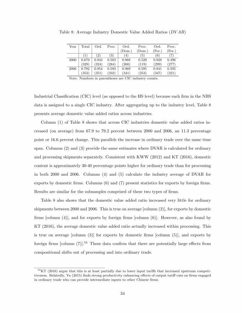
Table 8: Average Industry Domestic Value Added Ratios (DV AR)

Year Total Ord. Proc. Ord. Proc. Ord. Proc.(Dom.) (Dom.) (For.) (For.)

(1) (2) (3) (4) (5) (6) (7)

2000 0.679 0.944 0.503 0.968 0.529 0.928 0.496(329) (324) (284) (260) (119) (299) (277)

2006 0.792 0.954 0.593 0.969 0.595 0.941 0.595(352) (351) (332) (341) (253) (347) (321)

Note: Numbers in parentheses are CIC industry counts.

Industrial Classification (CIC) level (as opposed to the HS level) because each firm in the NBS

data is assigned to a single CIC industry. After aggregating up to the industry level, Table 8

presents average domestic value added ratios across industries.

Column (1) of Table 8 shows that across CIC industries domestic value added ratios in-

creased (on average) from 67.9 to 79.2 percent between 2000 and 2006, an 11.3 percentage

point or 16.6 percent change. This parallels the increase in ordinary trade over the same time

span. Columns (2) and (3) provide the same estimates where DVAR is calculated for ordinary

and processing shipments separately. Consistent with KWW (2012) and KT (2016), domestic

content is approximately 30-40 percentage points higher for ordinary trade than for processing

in both 2000 and 2006. Columns (4) and (5) calculate the industry average of DVAR for

exports by domestic firms. Columns (6) and (7) present statistics for exports by foreign firms.

Results are similar for the subsamples comprised of these two types of firms.

Table 8 also shows that the domestic value added ratio increased very little for ordinary

shipments between 2000 and 2006. This is true on average [column (2)], for exports by domestic

firms [column (4)], and for exports by foreign firms [column (6)]. However, as also found by

KT (2016), the average domestic value added ratio actually increased within processing. This

is true on average [column (3)] for exports by domestic firms [column (5)], and exports by

foreign firms [column (7)].54 These data confirm that there are potentially large effects from

compositional shifts out of processing and into ordinary trade.

54KT (2016) argue that this is at least partially due to lower input tariffs that increased upstream competi-tiveness. Relatedly, Yu (2015) finds strong productivity enhancing effects of output tariff cuts on firms engagedin ordinary trade who can provide intermediate inputs to other Chinese firms.

34

Table 9: Input Tariffs and Domestic Value Added Ratios

Dep. Var. Dep. Var. Dep. Var.∆ ln(DV ARipt) ∆DV ARipt %∆DV ARipt(1) (2) (3) (4) (5) (6)

∆ ln(τI,it

)-0.51∗∗ -0.28 -0.25∗∗ -0.19∗ -0.48∗∗ -0.33(0.24) (0.27) (0.10) (0.11) (0.20) (0.20)

∆ ln(SO,ipt) 0.17∗∗∗ 0.058∗∗∗ 0.12∗∗∗

(0.03) (0.01) (0.02)ln (Si/Ui) -0.24 -0.19 -0.19∗∗ -0.18∗∗ -0.24 -0.22

(0.19) (0.19) (0.08) (0.08) (0.16) (0.15)ln (Ki/Li) 0.37∗∗ 0.14 0.13∗ 0.053 0.28∗∗ 0.11

(0.17) (0.15) (0.07) (0.06) (0.14) (0.11)%Diffi 0.23 -0.048 0.16 0.081 0.26 0.094

(0.26) (0.27) (0.11) (0.10) (0.21) (0.20)∆ ln

(DDit /D

Xit

)-0.015 -0.0038 0.018 0.023 0.0047 0.017(0.06) (0.05) (0.03) (0.02) (0.05) (0.04)

Obs. 1,596 1,535 1,633 1,549 1,633 1,549L-Cens. . . 1 1 2 1Non-Cens. . . 1631 1548 1596 1535R-Cens. . . 1 0 35 13

Columns (1)-(2) are WLS. Columns (3)-(6) are two-sided Tobits with censoringvalues of -1 and 1 in columns (3) and (4), and -2 and 2 in columns (5) and (6).Dependent variables given at the top of each column. Standard errors inparentheses are clustered at the IO level. All regressions include province fixedeffects p < 0.01 :∗∗∗, 0.01 ≤ p < 0.05 :∗∗, 0.05 ≤ p < 0.10 :∗. Regressionsweighted by the number of firms for each ip observation.

7.2 Industry Level Evidence

We now explicitly examine the link between lower input tariffs and domestic value added ratios.

Analogous to section 5, we conduct our analysis at the CIC industry-province level so as to

allow for geographic heterogeneity. With slight abuse of notation, CIC industries are indexed i

and provinces are indexed p. Our starting point is equation (11), where the dependent variable

is the log difference of the domestic value added ratios:

∆ ln(DV ARipt) = β1∆ ln(τI,it) + β′XXi + Φp + µipt. (11)

Industry-level input tariffs are the same as before, while the vector Xi contains the same

control variables as in section 5. We continue to cluster the standard errors at the IO industry

level and weight observations as before. Equation (12) includes the (log) change in the share

of ordinary trade as an additional control:

∆ ln(DV ARipt) = β1∆ ln(τI,it) + β2∆ ln(SO,ipt) + β′XXi + Φp + µipt. (12)

35

If the effect of input tariff cuts on DVAR is coming through the organization of trade, we

expect any effect of ∆ ln(τI,it) in equation (11), to be mitigated or eliminated entirely when

the share of ordinary trade is included directly in equation (12).

Column (1) of Table 9 presents results from estimating equation (11) and column (2) adds

the share of ordinary trade to estimate equation (12). Columns (3) and (4) present Tobit

results when the dependent variable is in first differences (∆DV ARipt). Columns (5) and (6)

present results using proportional changes [%∆DV ARipt].55

Column (1) finds that a 1 log point cut in input tariffs causes a 0.51 log point increase in

the domestic value added ratio, consistent with the results in section 5 and a higher measured

DVAR in ordinary relative to processing trade. The inclusion of the share of ordinary trade

[column (2)] reduces the point estimate on input tariffs by about half and increases the standard

error so that the effect is no longer statistically significant. There is, however, a very strong

and significant relationship between the (log) change in the share of ordinary trade and the

change in the DVAR as suggested by the data in Table 8. Columns (3)-(6) show that this

qualitative result is unchanged under alternative functional form assumptions although input

tariffs maintain a marginal significance in column (4).

While it is tempting to argue that lower input tariffs increased total demand for domestic

factors of production, this does not follow from our analysis for two reasons. First, our empirical

strategy that compares first differences only identifies relative effects and not aggregate effects.

Second, the analysis only examines the domestic value added ratio of exports and not total

production.

Interestingly, while imprecisely estimated, the point estimate on input tariffs remains nega-

tive in columns (2), (4), and (6), which directly control for the change in the share of ordinary

trade. One might expect substitution effects to appear in our results as a positive coefficient

on input tariffs after controlling for the share of ordinary trade. Specifically, there might be

both between and within effects, where the between effect is the reallocation of production

from processing to ordinary trade, which implies an increase in DVAR, and the within effect

is that producers in the ordinary trade regime should decrease their DVAR. Once we control

55Where %∆DV ARipt ≡ DVARip,2006−DVARip,2000

0.5∗[DVARip,2006+DVARip,2000]

36

for the between effect, we might expect the within effect to appear in our results. However,

the point estimate on input tariffs remains negative even after controlling for the organization

of trade.

This behavior can be explained by patterns of pass-through and productivity upgrading in

China. Brandt et al. (2016) find relatively high degrees of pass-through from tariffs into prices

charged by domestic agents. Also, as documented by Han et al. (2016) foreign (e.g. US) firms

capture some of the tariff cuts into higher prices. Such high degrees of pass-through into the

price of domestically provided inputs, combined with the partial capture of tariff cuts by foreign

firms mitigates possible substitution effects as discussed in section 3.6. Yu (2015) also finds

that reductions in output tariffs have substantial positive effects on the productivity of Chinese

firms. If productivity upgrading for Chinese firms causes the relative price of domestic inputs

to fall for processing firms (who do not directly benefit from falling tariffs), this is consistent

with rising domestic value added ratios for processing firms documented in Table 8 and KT

(2016).

8 Conclusion

This paper finds that a majority of the average change from processing to ordinary exports for

China between 2000 and 2006 can be explained by reductions in input tariffs with both the

intensive and extensive margins playing roles. In the cross-section, a larger domestic market

vis-a-vis export opportunities promoted the organization of ordinary exports. Over the period

we examine however, the relative value of accessing the domestic market actually declined as

world export markets grew more quickly than domestic absorption in China, which offset some

of the effect of falling tariffs on trade form. A reversal in this behavior due to the Great Trade

Collapse following the Great Recession in 2008 may explain the more recent sharp decline in

the role of processing.

Our finding that lower levels of protection for intermediate inputs did not cause domestic

value added ratios to fall might seem counter-intuitive. However, lower input tariffs in China

promoted the entry of new exporters who were more likely to export through ordinary trade

with higher domestic content. Falling input tariffs also encouraged incumbent firms to increase

37

their share of exports organized through ordinary trade, leading to higher shares of domestic

value added in gross exports through changes in export composition.

Assembly-intensive processing trade has played a strategic role in industrial upgrading and

export-led development for many countries (Radelet and Sachs, 1997 and Radelet, 1999). It is

a potentially important source of foreign exchange and foreign technology and know-how when

domestic markets are protected. However, processing trade also entails relatively lower demand

for domestic factors of production as documented here and elsewhere. Empirical assessment

of these trade-offs is an important area of research with regard to China and to development

policy in general. The reduced form mechanisms identified in this paper along with those in

other papers such as Yu (2015) and Manova and Yu (2016) can serve as the foundations for

more structural work that can provide full general equilibrium welfare assessments of processing

trade.

References

[1] Bai, Xue, Kala Krishna and Hong Ma, (2015) “How You Export Matters: Export Mode,Learning and Productivity in China,” NBER working paper #21164

[2] Bernard, Andrew B., J. Bradford Jensen, Stephen J. Redding and Peter K. Schott (2007)“Firms in International Trade,”Journal of Economic Perspectives, 21(3), 105-130

[3] Brandt, Loren, Johannes Van Biesebroeck, and Yifan Zhang (2012) “Creative Accountingor Creative Destruction: Firm Level Productivity Growth in Chinese Manufacturing,”Journal of Development Economics, 97(2), 339-351

[4] Brandt, Loren, Johannes Van Biesebroeck, Luhang Wang, and Yifan Zhang, (2016) “WTOAccession and Performance of Chinese Manufacturing Firms,” CEPR Discussion PaperNo. 9166 (October 2012, revised 2016)

[5] Branstetter, Lee and Nicholas R. Lardy, (2008) “China’s Embrace of Globalization” inChina’s Great Economic Transformation, Edited by Loren Brandt and Thomas G. Rawski,Cambirdge University Press, New York, 633-683

[6] Cameron, A. Colin, Jonah B. Gelbach and Douglas L. Miller (2008) “Bootstrap-BasedImprovements for Inference with Clustered Errors,” Review of Economics and Statistics,90(3), 414-427

[7] Defever, Fabrice and Ajejandro Riano, (2012) “China’s Pure Exporter Subsidies,”workingpaper, University of Nottingham

38

[8] Feenstra, Robert C. and Gordon H. Hanson, (2005) “ Ownership And Control Of Out-sourcing To China: Estimating The Property-Rights Theory Of The Firm,” QuarterlyJournal of Economics, 120(2), 729-761

[9] Fernandes, Ana and Heiwai Tang (2012) “Determinants of vertical integration in exportprocessing: Theory and evidence from China,” Journal of Development Economics, 96(2),396-414

[10] Haltiwanger, John and Ron S. Jarmin and Javier Miranda, (2013) “Who Creates Jobs?Small versus Large versus Young,” The Review of Economics and Statistics,. 95(2), pages347-361

[11] Han, Jun, Runjuan Liu, Beyza Ural Marchand, and Junsen Zhang, (2016) “Market Struc-ture, Incomplete Tariff Pass-through, and Household Welfare in Urban China,” Journalof International Economics, forthcoming

[12] Hanson, Gordon, (2012) “The Rise of Middle Kingdoms: Emerging Economies in GlobalTrade,” Journal of Economic Perspectives, 26(2), 41-64

[13] Helpman, Elhanan, Marc J. Melitz, and Stephen Yeaple (2004) “Export Versus FDI withHeterogeneous Firms, American Economic Review, 94(1), 300-316

[14] Jarreau, Joachim and Sandra Poncet, (2012) “Export sophistication and economic growth:Evidence from China,” Journal of Development Economics, 97(2), 281-292.

[15] Johnson, Robert C. and Guillermo Noguera, (2016) “Fragmentation and Trade in ValueAdded over Four Decades,” NBER Working Paper #18186, National Bureau of EconomicResearch, Inc.

[16] Kee, Hiau Looi and Heiwai Tang, (2016) “Domestic Value Added in Exports: Theory andFirm Evidence from China,” American Economic Review, 106(6) 1402-1436

[17] Koopman, Robert, Zhi Wang, and Shang-Jin Wei (2012) “Estimating domestic content inexports when processing trade is pervasive,” Journal of Development Economics, 96(2),178-189

[18] Kroszner, Randall S., Luc Laevenb and Daniela Klingebield (2007) “Banking crises, fi-nancial dependence, and growth,” Journal of Financial Economics, 84(1), 187228

[19] Levinsohn, James, (1999) “Employment responses to international liberalization in Chile,”Journal of International Economics, 47(2), 321-344.

[20] Madini, Dorsati, (1999) “A Review of the Role and Impact of Export Processing Zones,”World Bank, Policy Research Working Paper #2238

[21] Manova, Kalina and Zhihong Yu, (2016) “Firms and Credit Constraints along the ValueChain: Processing Trade in China,”Journal of International Economics, Vol. 100(C), 120-137

[22] Melitz, Marc J., (2003)“The Impact of Trade on Intra-Industry Reallocations and Aggre-gate Industry Productivity,” Econometrica, 71(6), 1695-1725.

39

[23] Naughton, Barry (1996) “China’s Emergence and Prospects as a Trading Nation,” Brook-ings Papers on Economic Activity , Vol. 2, 273-344

[24] Nunn, Nathan, (2007) “Relationship-Specificity, Incomplete Contracts, and the Patternof Trade,” Quarterly Journal of Economics, 122(2), 569-600

[25] Radelet, Steven, (1999) “Manufactured Exports, Export Platforms, and EconomicGrowth,” Harvard Institute for International Development working paper

[26] Radelet, Steven and Jeffrey Sachs (1997) “Asia’s Reemergence,” Foreign Affairs, 76(6),44-59

[27] Yi, Kei-Mu, (2003) “Can Vertical Specialization Explain the Growth of World Trade?,”Journal of Political Economy, 111(1), 52-102

[28] Yu, Miaojie, (2015) “Processing Trade, Tariff Reductions and Firm Productivity: Evi-dence from Chinese Firms,” Economic Journal, 125(585), 943-988

A Domestic Absorption Calculation

For years t ∈ {1995, 2004, 2008}, we calculate domestic absorption as follows where Qit is thevalue of production, Mit is the value of imports into China, and Xit is the value of exportsfrom China in CIC industry i:

DDit ≡ Qit +Mit −Xit.

Qit is available at the CIC level but is only available for census years. We use UN COMTRADEtrade data for the years 1995, 2004, and 2008 in the calculation above. These trade data arecollected at the HS level and then aggregated to the CIC level. In cases where a given six-digitHS code maps into multiple CIC codes, shares are allocated based on the output size of theCIC industries. We then calculate the average growth rate of this variable for two windows1995-2004 and 2004-2008 where Tt′−t is the number of years in each window between years t′

and t:

gi,1995−2004 =ln(DDi,2004

)− ln

(DDi,1995

)T2004−1995

gi,2004−2008 =ln(DDi,2008

)− ln

(DDi,2004

)T2008−2004

.

We then impute the interim years according to the following formula

DDi,2000 ≡ DD

i,1995 ∗ (1 + gi,1995−2004)5

DDi,2003 ≡ DD

i,1995 ∗ (1 + gi,1995−2004)8

DDi,2006 ≡ DD

i,2004 ∗ (1 + gi,2004−2008)2

The ratio of domestic absorption to external demand is the ratio of DDi,t to Chinese exports at

the CIC level for the years 2000, 2003, and 2006. Log differences are the difference betweenthe (log) 2006 and 2000 values.

40

B Decomposition Details

Start by defining the proportional change in the share of ordinary trade as

%∆SO,ipt =SO,ip,2006 − SO,ip,2000

0.5 ∗ [SO,ip,2006 + SO,ip,2000]=

VO,ip,2006Vip,2006

− VO,ip,2000Vip,2000

0.5 ∗ [SO,ip,2006 + SO,ip,2000].

Decomposing this into export values accruing to domestic and foreign firms, we obtain

%∆SO,ipt =

V DO,ip,2006Vip,2006

− V DO,ip,2000Vip,2000

0.5 ∗ [SO,ip,2006 + SO,ip,2000]︸︷︷︸DOMO,ipt

+

V FO,ip,2006Vip,2006

− V FO,ip,2000Vip,2000

0.5 ∗ [SO,ip,2006 + SO,ip,2000]︸︷︷︸FORO,ipt

.

The first term provides us with the dependent variable in column (2) of Table 6 and the secondprovides us with the dependent variable in column (3) of Table 6. To decompose further into

the incumbent, new firm, and exiting firm margins, define V D,kO,ip,2006 as ordinary exports by

domestic firms in group k ∈ {I,N,E} (as described in the text), we obtain

%∆SO,ipt =∑k

V D,kO,ip,2006

Vip,2006− V D,kO,ip,2000

Vip,2000

0.5 ∗ [SO,ip,2006 + SO,ip,2000]+∑k

V F,kO,ip,2006

Vip,2006− V F,kO,ip,2000

Vip,2000

0.5 ∗ [SO,ip,2006 + SO,ip,2000].

Therefore we obtain

%∆SO,ipt = DOM IO,ipt +DOMN

O,ipt +DOMEO,ipt + FORIO,ipt + FORNO,ipt + FOREO,ipt

where, setting 2006 values to zero for exiting firms and 2000 values to zero for new firms, weobtain the following values for the decomposition for domestic and foreign incumbent, new,and exiting firms (respectively):

DOM IO,ipt =

V D,IO,ip,2006

Vip,2006− V D,IO,ip,2000

Vip,2000

0.5 ∗ [SO,ip,2006 + SO,ip,2000]FORIO,ipt =

V F,IO,ip,2006

Vip,2006− V F,IO,ip,2000

Vip,2000

0.5 ∗ [SO,ip,2006 + SO,ip,2000]

DOMNO,ipt =

V D,NO,ip,2006

Vip,2006

0.5 ∗ [SO,ip,2006 + SO,ip,2000]FORNO,ipt =

V F,NO,ip,2006

Vip,2006

0.5 ∗ [SO,ip,2006 + SO,ip,2000]

DOMEO,ipt = −

V D,EO,ip,2000

Vip,2000

0.5 ∗ [SO,ip,2006 + SO,ip,2000]FOREO,ipt = −

V F,EO,ip,2000

Vip,2000

0.5 ∗ [SO,ip,2006 + SO,ip,2000]

C Baseline Estimation for Domestic and Foreign Firms

This section examines our baseline results by looking at subsamples of domestic and foreignfirms. This section is not a formal decomposition of the overall effect (as found in the mainbody of the text). Rather, it is a “within” exercise that examines whether the forces identifiedin Table 2 hold within subsamples of each type of firm. To do this, start by defining the shareof ordinary exports by domestic firms as

41

Table 10: Domestic Firms Subsample

Dep. Var: Dep. Var:

ln(SDO,ipt

)∆ ln

(SDO,ipt

)2000 2000 2003 2003 2006 2006 2000-2006(1) (2) (3) (4) (5) (6) (7) (8)

ln(τI,it

)-2.41∗ -1.37∗ -1.44∗ -1.06∗ -0.91 -0.85∗∗

(1.35) (0.82) (0.87) (0.58) (0.56) (0.42)∆ ln

(τI,it

)-0.95∗∗∗ -0.74∗∗∗

(0.22) (0.24)ln

(DDit /D

Xit

)0.31 0.25 0.12

(0.22) (0.20) (0.11)∆ ln

(DDit /D

Xit

)0.065∗

(0.03)%Diffi -1.07 -1.19 -0.89 -0.050

(0.86) (0.79) (0.56) (0.12)ln (Si/Ui) 0.080 -0.17 -0.30 0.15

(0.94) (0.56) (0.27) (0.12)ln (Ki/Li) -0.011 -0.19 -0.038 -0.15


Columns (1)-(6) are one-sided Tobits with an (upper) censoring value of ln(1) = 0.Columns (7)-(8) are WLS. Dependent variables are at the top of each column. Standarderrors in parentheses are clustered at the IO level. All regressions include province fixedeffects. p < 0.01 :∗∗∗, 0.01. ≤ p < 0.05 :∗∗, 0.05 ≤ p < 0.10 :∗. Regressions weighted bythe number of firms for each ip observation.

SDO,ipt =V DO,ipt

V Dipt

where V Dipt is total exports by domestic firms in the triplet ipt and V D

O,ipt is exports throughordinary trade for the same triplet. An analogous expression holds for the share of ordinaryexports by foreign firms SFO,ipt. Tables 10 and 11 present results for these subsamples. Noticethat these are not formal decompositions but rather “within” samples that allow us to examinethe mechanisms at play for these two types of firms separately.

D Alternative Functional Forms

First, we redefine our dependent variable in the cross-section as SO,ipt and in the time series as

%∆SO,ipt =SO,ip,2006−SO,ip,2000

0.5∗[SO,ip,2006+SO,ip,2000]. For the cross-sectional results, the dependent variable is

bound in the interval [0,1] and we therefore use a two-sided Tobit with a lower censoring valueof 0 and an upper censoring value of 1. Results in the cross-section appear in column (1)-(6)of Table 12. Columns (7) and (8) present proportional changes where the left censoring is at%∆SO,ipt = −2 and the upper censoring is at %∆SO,ipt = 2. Qualitative results are unchangedfrom our main specification. Columns (9) and (10) estimate equation (9) when the dependentvariable is defined in first differences [∆SO,ipt = SO,ip,2006−SO,ip,2000] such that the dependent

42

Table 11: Foreign Firms Subsample

Dep. Var: Dep. Var:

ln(SFO,ipt

)∆ ln

(SFO,ipt

)2000 2000 2003 2003 2006 2006 2000-2006(1) (2) (3) (4) (5) (6) (7) (8)

ln(τI,it

)-2.15∗∗∗ -1.45∗∗∗ -1.06∗∗∗ -0.86∗∗ -0.78∗∗ -0.87∗∗∗

(0.39) (0.53) (0.33) (0.34) (0.31) (0.28)∆ ln

(τI,it

)-2.08∗∗∗ -1.79∗∗∗

(0.68) (0.68)ln

(DDit /D

Xit

)0.29∗∗∗ 0.26∗∗∗ 0.20∗∗∗

(0.09) (0.08) (0.07)∆ ln

(DDit /D

Xit

)0.11∗∗

(0.05)%Diffi -1.94∗∗∗ -2.05∗∗∗ -1.48∗∗∗ 0.28

(0.70) (0.56) (0.45) (0.30)ln (Si/Ui) -1.60∗∗ -1.24∗∗∗ -1.08∗∗∗ -0.066

(0.69) (0.48) (0.37) (0.35)ln (Ki/Li) 0.58 0.22 0.13 0.060


Columns (1)-(6) are one-sided Tobits with an (upper) censoring value of ln(1) = 0.Columns (7)-(8) are WLS. Dependent variables are at the top of each column. Standarderrors in parentheses are clustered at the IO level. All regressions include province fixedeffects. p < 0.01 :∗∗∗, 0.01. ≤ p < 0.05 :∗∗, 0.05 ≤ p < 0.10 :∗. Regressions weighted bythe number of firms for each ip observation.

variable is bound between -1 and 1.56 Results are qualitatively similar across specifications.

56Because our baseline results are in proportional changes and the columns (9) and (10) are in first differences,their coefficients are not strictly comparable.

43

Table 12: Alternative Functional Forms

Dep. Var: Dep. Var: Dep. Var:SO,ipt %∆ (SO,ipt) ∆ (SO,ipt)

2000 2000 2003 2003 2006 2006 2000-2006 2000-2006

(1) (2) (3) (4) (5) (6) (7) (8) (9) (10)

ln (τI,it) -0.61∗∗∗ -0.36∗∗∗ -0.37∗∗∗ -0.27∗∗∗ -0.29∗∗∗ -0.29∗∗∗

(0.15) (0.13) (0.11) (0.10) (0.10) (0.09)∆ ln (τI,it) -0.66∗∗∗ -0.61∗∗

(0.21) (0.24)∆τIO,i -0.015∗ -0.0096∗∗

(0.01) (0.00)ln

(DDit /D

Xit

)0.066∗∗ 0.066∗∗ 0.045∗∗

(0.03) (0.03) (0.02)∆ ln

(DDit /D

Xit

)0.056∗∗ 0.00099(0.02) (0.01)

%Diffi -0.46∗∗∗ -0.48∗∗∗ -0.39∗∗∗ -0.053 -0.0018(0.18) (0.17) (0.13) (0.10) (0.05)

ln (Si/Ui) 0.053 -0.11 -0.22∗∗ -0.11 -0.18∗∗∗

(0.17) (0.13) (0.10) (0.12) (0.04)ln (Ki/Li) -0.063 -0.050 0.014 0.021 0.059∗∗

(0.21) (0.17) (0.13) (0.12) (0.02)

Obs. 31,276 31,276 39,427 39,427 47,772 47,564 27,687 27,597 27,746 27,655L-Cens. 842 842 500 500 366 365 95 95 60 60Non-Cens. 7,611 7,611 9,289 9,289 11,408 11,382 26,927 26,839 27,416 27,325R-Cens. 22,823 22,823 29,638 29,638 35,998 35,817 665 663 270 270

All regressions are two-sided Tobits with censoring values of 0 and 1 in columns (1)-(6), -2 and 2 in columns (7)and (8), and -1 and 1 in columnbs (9) and (10). Dependent variables given at the top of each column. Standarderrors in parentheses are clustered at the IO level. All regressions include province fixed effects. p < 0.01 :∗∗∗,0.01 ≤. p < 0.05 :∗∗, 0.05 ≤ p < 0.10 :∗. Regressions weighted by the number of firms for each ip observation.

44

E Construction of Domestic Content Ratios

Start with the accounting identity for a firm f operating in industry i:

Xfi = πfi + wfiLfi + rfiKfi +MDfi +M I

fi

where Xfi is the value of exports, πfi is profits from these exports, wfiLfi is total paymentsto labor in production of these exports, rfiKfi is total payments to capital for these exports,MDfi is total payments to domestically-provided intermediate inputs for these exports, and M I

fi

is total payments to imported intermediate inputs for these exports [KT (2016), equation (1)].Then decompose imported intermediate inputs into two mutually exclusive and exhaustivecomponents: foreign value added (qFfi) and domestic value added (through indirect channels)

(δDfi). Similarly, decompose domestically-provided intermediate inputs into domestic value

added (qDfi) and foreign value added (through indirect channels) (δFfi) (see their pg. 7). Thendefine domestic value added, DV Afi, as

DV Afi ≡ πfi + wfiLfi + rfiKfi + δDfi + qDfi.

Define XPfi and XO

fi as the value of processing and ordinary exports (respectively) for firm

f in industry i, and MPfi and MO

fi as analogous expressions for the value of imports. For aprocessing firm, KT show that domestic value added corresponds to:

DV APfi = XPfi −MP

fi + (δDfi − δFfi).

Following KT, we set δDfi = 0, and then use average values of δFfi from their Table Appendix

Table A7. This allows us to calculate domestic value added for a processing exporter DV APfi.

For an ordinary exporter, the calculation is slightly more complicated because one cannottell how total imports of intermediate inputs are allocated between production of exports anddomestically sold output. Following KT, we use a proportionality assumption where the ratioof intermediate inputs used for ordinary exports to total intermediate inputs is assumed to beequal the ratio of ordinary exports to overall production for the firm. Arithmetically, whereY Dfi is domestic sales, Mfi is total imports, and Yfi = Y D

fi +Xfi is total output, this assumptionallows us to write domestic value added embodied in the exports of an ordinary exporter:

DV AOfi = XOfi −MO

fi + (δDfi − δFfi)

where

MOfi = Mfi

[1−

Y Dfi

Yfi

].

Industry domestic value added in exports is then equal to the sum of domestic value added inordinary exports and processing exports across all firms in an industry i:

DV Ai =∑

f∈Si;j∈{O,P}

DV Ajfi.

where Si is the set of all firms in industry i. The ratio of domestic value added in exports to

45

gross exports is then equal to this value divided by total exports:

DV ARi =

∑f∈Si;j∈{O,P}DV A

jfi.∑

f∈Si;i∈{O,P}Xjfi

.

46

Tari s and the Organization of Trade in China s and the Organization of Trade in China Loren Brandt...

Documents

Transcript of Tari s and the Organization of Trade in China s and the Organization of Trade in China Loren Brandt...