Staff Working Paper ERSD-2018-10 26 October 2018 ______________________________________________________________________

World Trade Organization

Economic Research and Statistics Division

______________________________________________________________________

The “China Shock” revisited: Insights from value added trade

flows*

Adam Jakubik

World Trade Organization, Geneva

Victor Stolzenburg World Trade Organization, Geneva

Manuscript date: 26 October 2018

______________________________________________________________________________ Disclaimer: This is a working paper, and hence it represents research in progress. The opinions expressed in this paper are those of the authors. They are not intended to represent the positions or

opinions of the WTO or its members and are without prejudice to members' rights and obligations under the WTO. Any errors are attributable to the authors.

* The authors wish to thank David Dorn, Bernard Hoekman, Robert Koopman, Marc-Andreas Muendler, Marcelo Olarreaga, Stela Rubinova, Peri Silva, Jens Suedekum, Thierry Verdier, Aksel Erbahar, and participants at NCCR Trade Regulation Brown Bag Series, World Trade Institute, University of Bern; Geneva Trade and Development Workshop, Graduate Institute of International and Development Studies; ILO Research Seminar; ETSG 2017; ELSNIT; Sixth IMF-WB-WTO Trade Conference at the International Monetary Fund; Bank of Canada Research Seminar; RMET 2018; IOSE 2018; and APTS 2018 for helpful comments and suggestions and are especially grateful to Zhi Wang and colleagues at RCGVC, UIBE for providing data on the value added decomposition of trade flows. The opinions expressed in this paper should be attributed to its authors. They are not meant to represent the positions or opinions of the WTO and its Members and are without prejudice to Members’ rights and obligations under the WTO.

The “China Shock” revisited: Insights from value added tradeflows∗

Adam Jakubik† Victor Stolzenburg‡

October 26, 2018

Abstract

We exploit a decomposition of gross trade flows into their value added components to re-assess the relationship between increased imports from China and manufacturing jobs in USlocal labour markets following the seminal paper of Autor, Dorn, and Hanson (2013, ADH).Decomposed trade flows enable us to address identification and measurement issues inherentto gross trade data. In particular, it allows us to remove US value added in Chinese exportsfrom the exposure measure which is mechanically correlated with the dependent variable andoverstates the volume of the trade shock. In addition, the decomposition permits to correctfor double counting, to remove primary and services inputs in manufacturing exports, andto assign competition to the upstream industry that supplied the value added rather thanthe final exporting industry. This further reduces the volume of the shock and improves theaccuracy of the import exposure measure. Consequently, we find considerable differencesin the pattern of regions that are most affected by the trade shock and show that importsfrom China can explain less of the decline in US manufacturing than what gross trade datawould suggest. We then separate the shock into a China-driven domestic reform and a third-country-driven value chain component, and find in line with ADH that the smaller, but stillnegative labour market effects are indeed China driven. Finally, we observe that the negativeeffects identified in ADH are not present in the 2008-2014 period, as labour market adjust-ment has largely concluded. The long time needed for adjustment may have been prolongedby the evolution of China’s comparative advantage.

Keywords: value added trade, labor-market adjustment, local labor marketsJEL Classification: E24; F14; F16; J23; L60; R23

∗The authors wish to thank David Dorn, Bernard Hoekman, Bob Koopman, Marc-Andreas Muendler, MarceloOlarreaga, Stela Rubinova, Peri Silva, Jens Suedekum, Thierry Verdier, Aksel Erbahar, and participants at NCCRTrade Regulation Brown Bag Series, World Trade Institute, University of Bern; Geneva Trade and DevelopmentWorkshop, Graduate Institute of International and Development Studies; ILO Research Seminar; ETSG 2017;ELSNIT; Sixth IMF-WB-WTO Trade Conference at the International Monetary Fund; Bank of Canada ResearchSeminar; RMET 2018; IOSE 2018; and APTS 2018 for helpful comments and suggestions and are especiallygrateful to Zhi Wang and colleagues at RCGVC, UIBE for providing data on the value added decomposition oftrade flows. The opinions expressed in this paper should be attributed to its authors. They are not meant torepresent the positions or opinions of the WTO and its Members and are without prejudice to Members’ rightsand obligations under the WTO.

†World Trade Organization, Geneva; E-mail: adam.jakubik@wto.org.‡World Trade Organization, Geneva; E-mail: victor.stolzenburg@wto.org.

1

1 Introduction

The reintegration of China into the world trading system has been an extraordinary historicalachievement that has lifted millions of people out of poverty. It has also set in motion monumentalshifts in world trading patterns which provide a unique opportunity to examine the effects of tradepolicy. This research has found evidence of lower prices and greater investment in innovationdue to trade with China (Feenstra and Weinstein, 2017; Amiti et al., 2017; Bloom et al., 2016;Impullitti and Licandro, 2018). On the flip side, trade liberalisation necessitates adjustments inboth factor and product markets. As is the case with adjustment due to technological progress orchanges in consumer tastes, some individuals will be worse off than before and can face significantadversities in transitioning from job to job. While the gains from trade through lower prices arerelatively evenly distributed throughout the US, the patterns of geographical clustering typicalof manufacturing industries cause local communities to be asymmetrically affected by importcompetition. Highly influential research by Autor et al. (2013, henceforth ADH) shows thatUS local labour markets more exposed to increased import competition from China have seensignificant losses in jobs and earnings relative to less exposed labour markets. These effects havealso been shown to be present in other advanced economies such as Spain, Norway, and France(Donoso et al., 2015; Balsvik et al., 2015; Malgouyres, 2016).

Although recent research suggests that these negative effects are not present at the national level,and that the cost savings made possible by trade with China have actually helped industries retainworkers on aggregate (Caliendo et al., 2015; Magyari, 2017; Wang et al., 2017), this does notdiminish the significance of the fact that in many locations US manufacturing industries havesuffered, and further research by Adda and Fawaz (2017) and Autor et al. (forthcoming) shownegative effects in other areas of life of those affected, such as health and marriage prospects.The localised pain felt by those adversely impacted has started to feed into the political processand has shaped the discourse on trade at a national level. Colantone and Stanig (2016) show thatthe vote for Brexit was influenced by import competition from China, and Autor et al. (2017)present evidence on trade with China contributing to the polarisation of US politics. In lightof these developments, researchers and policy makers have emphasized the need for adjustmentpolicies, such as place-based or mobility policies, in order to secure the net welfare gains fromtrade while minimizing the hardship for locations and individuals who are affected negatively bytrade (IMF, World Bank, WTO, 2017; WTO, 2017; Austin et al., 2018). For such policies it iscrucial to correctly identify which regions and sectors are exposed to import competition and towhat extent.

In this paper, we firstly show that the statistical concept of trade in value added can greatlyenhance the accuracy of import competition measures with important consequences for the spatialdistribution and the magnitude of trade shocks. Moreover, value added decomposed trade flowsfurther allow us to correct for a mechanically endogenous component of the exposure measure,namely US value added in Chinese exports, and to distinguish between the impact of China-specific drivers of the trade shock and that of third countries who use China in final stages oftheir production but provide much of the value added. The final contribution of this paper is toexplore the length of adjustment and how changes in China’s comparative advantage over time

2

may have prolonged the employment effects.

We address these questions by exploiting data from Inter-Country Input-Output tables (ICIOs)covering the time period from 2000 to 2015. This expands the time-period analysed by ADH toshed light on whether the negative effect of Chinese import competition persists, and thereforewhether the China shock is fundamentally different from other trade shocks with regard toadjustment time. The tables allow splitting gross imports from China into their individual valueadded components by origin and, thus, separate Chinese value added (which we refer to asdomestic value added, DVA) in exports to the US from third country value added (foreign valueadded, FVA) that enters the US via China. This approach entails two important methodologicalimprovements over the use of gross export data.

Firstly, it allows us to create a more precise measure of local labour market exposure by ad-dressing four different measurement issues of gross imports. Goods exported from a downstreamindustry such as consumer electronics contain inputs from upstream industries such as plasticsand fabricated metal products. Therefore, a rise in US consumer electronics imports might ac-tually affect local labour markets which depend on plastics or fabricated metal products. Forinstance, let us assume that ten people are required to produce a mobile phone but only five ofthem actually work in the electronics industry while the other five are employed by the glass,plastics and other upstream industries that are located elsewhere. This means that when amobile phone is imported, gross trade data incorrectly assigns 50% of the competition by as-signing it fully to the electronics industry and the local labour markets where that industry isrepresented. In addition, gross imports hide the fact that certain upstream production stagesof imported goods might still be performed at home. Using the mobile phone as example, itmight be that two employees are in charge of high-tech components and while the other stagesare off-shored, high-tech production stages remain domestic. In this case gross trade data wouldoverstate exposure by 20%. Similarly, many goods are dependent on primary and services inputsand as long as the focus is on manufacturing employment as in this paper or ADH, such inputsshould be excluded which is possible with value added data. Finally, in the age of value chainsgross trade data suffers from double counting when intermediates cross the same border twice. Iffor example, China produces phone cases and ships them to the US where high-tech componentsare inserted before the phone travels back to China for final assembly, then the phone case wouldbe counted twice by gross trade data. By looking at the value added content of US importsfrom China, we can address these four issues and correctly assign the imports to the local labourmarkets that are ultimately affected.

The second methodological improvement relates to another measurement issue, namely US valueadded in Chinese exports. Value added trade data allows us to better control for the endogeneityof import exposure by removing the US value added component in Chinese exports. Since USemployment is a major contributor to US value added in Chinese exports, there is a mechanicalcorrelation between import exposure and employment in manufacturing. This mechanical cor-relation is not addressed by the instrumentation strategy of ADH since US value added is alsopresent in Chinese exports to other high-income countries. By removing this part of Chineseexports, we improve the validity of the instrument. Johnson and Noguera (2012) show that the

3

US value added content in Chinese exports is considerable which highlights that this adjustmentis quantitatively meaningful and relevant.

Turning to our results, we find that using value added instead of gross trade flows changes thegeography of import competition considerably. As expected, locations specialized in downstreamindustries, in particular electrical machinery and electronic equipment, are much less exposed toimport competition than what gross imports would suggest while the opposite hold for certainlocations specialized in upstream manufacturing including steel. Two of our most extreme casesin this regard are San Jose, California, home to Silicon Valley and many of the US’ main electronicequipment manufacturers, and North-West Indiana, home to the largest steel mill in the US andlarge aluminum producers. In these commuting zones, import competition in value added termsis more than a standard deviation different from gross import exposure. In the case of SanJose the exposure decreases while it increases for North-West Indiana. These intuitive resultshighlight the need to take value added data into account when assessing the geography of tradeshocks and when designing policy responses, in particular when these policies are place-based.They also facilitate our understanding of current trade policy developments since they alignimport competition more closely with certain recently introduced trade policy measures.

Next, we find that Chinese import competition can explain less of the US manufacturing declinethan previously considered. As using value added imports effectively reduces measurement errorwhich biases estimates towards zero and corrects for an upward bias introduced by endogeneity,we observe that the corresponding coefficient on Chinese imports increases substantially com-pared to the coefficients obtained using gross import data. This speaks in favour of a larger roleof imports. However, since the total volume of the shock is significantly smaller once doublecounting, US value added, and primary and services inputs are excluded, we find that the totalnumber of jobs affected is in fact smaller than the corresponding gross trade number by 32.3%,despite the increased coefficient. This suggests that China has been relatively less important forthe decline of US manufacturing than what ADH find using gross trade flows.

Regarding the drivers behind the employment effects, we find that China-specific changes as sug-gested by ADH are dominant. Autor et al. (2016) discuss extensively the domestic reforms whichtook place in China that enabled it to integrate into the globalised economy as a manufacturingpowerhouse. At the same time, Johnson and Noguera (2016) and Koopman et al. (2012) researchthe proliferation of Global Value Chains (GVCs) and in particular the participation of China.Implications for US trade policy depend on the extent to which employment effects are causedby China-specific drivers as opposed to GVCs since the latter tend to be highly mobile and canreroute if faced with bilateral trade policy interventions. Our results show that for the period2000-2008 increased exposure to Chinese value added is associated with a relative decline in localmanufacturing employment, whereas exposure to foreign value added in Chinese exports has apositive effect, albeit not statistically significant. This means that US employment adjustmentsare caused by China-specific changes and not by indirect imports consistent with a GVC-drivenexplanation. The result for foreign value added suggests that other advanced economies suchas Japan and Korea re-routing exports via China does not harm US manufacturing. This ispotentially explained by lower prices of goods that have been previously imported by the US

4

directly from these countries boosting total demand without requiring significant new labourmarket adjustment in the industries affected. This hypothesis is in line with the fact that mostof foreign value added in Chinese exports to the US originates in high-income countries whichhave traded intensively with the US before the rise of China. An alternative hypothesis is thatforeign value added is associated more with horizontal intra-industry trade and Chinese valueadded with vertical intra-industry trade as defined by Greenaway et al. (1995), and hence theformer necessitates relatively little labour market adjustment.

Finally, we find that in the period from 2008-2014 the negative effects of local exposure to Chi-nese value added are no longer present. The corresponding coefficients in this latter period areno longer statistically significant, implying that the China shock today is not driving regionaldifferences in manufacturing employment. We further split the Chinese value added exposurealong three industry groups to determine if the negative impact is driven by a particular subsetof industries. Specifically, the three groups comprise industries in which China has had a com-parative advantage since 1995, industries in which China had gained a comparative advantagebetween 1995 and 2008, and industries in which China has had a comparative disadvantage be-tween 1995 and 2008. We find that in the period 2000-2008 exposure to value added from thefirst two groups is associated with negative effects on local manufacturing employment, however,in 2008-2014 these are no longer statistically significant. This implies that adjustment has takenplace in industries where China has had or relatively recently gained a competitive edge, andthat it has concluded. Exposed occupations and firms have contracted or adapted successfully,leaving the surviving manufacturing occupations and firms largely resistant to a further increasein import competition. While the adjustment period estimated by ADH of about 10 years fromthe mid-1990s to 2007 is fairly long, this is consistent with the concurrent evolution of China’scomparative advantage to encompass more complex and skill intensive manufacturing industries.We conclude that policy measures aimed at limiting imports from China cannot be vindicatedby the aim of protecting manufacturing employment.

The rest of this paper is organised as follows. Section 2 reviews the related literature, Section3 discusses the data followed by Section 4 on the empirical strategy, Section 5 presents theeconometric results, and Section 6 concludes.

2 Related Literature

Our work is directly related to the seminal paper by ADH and papers that replicate their method-ology (e.g. Dauth et al., 2014; Balsvik et al., 2015; Malgouyres, 2016). Our methodological con-tribution to this line of research is to improve upon the identification as well as the precision ofthe exposure measure by considering also the upstream industries and countries that contributevalue added to the final product whose industry is recorded in the gross trade statistics.

In addition, our work is similar in spirit to Shen and Silva (2018) who also adopt a value addedperspective. Rather than studying the value added decomposition of bilateral gross trade flows,they view the impact of the rise of China through a different lens, focusing on all the Chinese value

5

added that is eventually absorbed by the US. That is, they exclude foreign value added in Chineseexports to the US but consider instead also the Chinese value added embedded in third countryexports to the US. For instance, China might export processed rare earth elements to Japan forthe production of semiconductors which are then exported to the US. In technical terms, thevalue added decomposition we use employs backward linkages whereas their’s employs forwardlinkages. While this is a very valuable exercise, their decomposition is not suited to provideinsights for bilateral trade policy and does not allow for a direct comparison to the results byADH who, like us, look at bilateral trade flows.

Similar to our paper, more recent work on the impact of Chinese imports emphasises the im-portance of input-output linkages (e.g. Acemoglu et al., 2016; Wang et al., 2017). Acemogluet al. (2016) use industry level data to complement the effects of direct industry exposure withexposure which propagates downstream to a given industry’s customers and exposure whichpropagates upstream to a given industry’s suppliers. As one would expect, direct and upstreameffects of exposure are found to be negative, however downstream effects are statistically in-significant. While related to our approach in spirit, they continue to rely on gross trade datato calculate the direct exposure measures and based on these direct exposure measures estimateindirect exposure using US national input-output tables. This means that the measurement andidentification issues mentioned above are not addressed in their work and affect their direct andindirect measures. In contrast, like ADH, we are interested only in the direct exposure measure.By taking into account foreign, as opposed to US, input-output linkages we are able to capturethe direct exposure effects more precisely by shifting some import competition to the upstreamindustries that are affected. However, this still only relates to direct exposure and is thus notcomparable to the approach in Acemoglu et al. (2016) or Wang et al. (2017), who define directexposure similarly. In contrast to Acemoglu et al. (2016), Wang et al. (2017) find statisticallysignificant positive downstream effects since they calculate downstream exposure using importsof only intermediate goods and services. Once effects on services sectors are taken into account,they find that the net effect of trading with China on local employment is modestly positive.

The effects we identify here are but one side of the coin of trade liberalisation: the necessarylocal labour market adjustment. Magyari (2017) broadens the focus by studying the effects onUS manufacturing employment at a firm level, cutting across local labour markets. She findsthat US firms involved in manufacturing record net gains in jobs in response to increased Chineseimport competition. While specific units of production within the firm shrink, others, in sectorswhere the US has a comparative advantage relative to China experience employment growth.These results are attributed to firms reorganising production and a favourable cost shock inthe form of cheaper Chinese inputs. This does not contradict the significant effects found ata local labour market level or indeed the adjustment costs faced by individual workers, rather,this methodology is suited to assess the aggregate effects of a trade shock, which are equallyimportant to consider from a policy perspective.

In one of the earliest papers in trade to apply this type of identification strategy, Topalova(2007) emphasises that this methodology is suited to identify short- and medium-run effects atthe local level. Rather than identifying the effects of the treatment, in our case the China shock,

6

on the national aggregate levels of the outcome variable, the focus is on identifying differentialregional effects based on regional variation in the level of treatment exposure. The fact thatmanufacturing employment is reduced more in local labour markets that are more exposed toimport competition is a good indicator of the locally borne costs of trade adjustment, which aregreatly important for domestic policy, as discussed earlier. However, it is not informative aboutthe causal effects of the China shock on the manufacturing employment share at a national level,much less about aggregate welfare implications in general equilibrium, which are more relevantquestions from a trade policy angle.

3 Data Description

We use value added decomposed trade flow data covering the years 2000 and 2007 generatedfrom the OECD ICIOs and based on the accounting framework proposed by Koopman et al.(2014) and further disaggregated to a bilateral-sector level by Wang et al. (2013). The databasecovers 61 countries and 34 industries.1 We prefer TiVA compared to alternative datasets sinceOECD and WTO have used elaborate techniques to deal with China’s processing trade. Due toChina’s outstanding role in GVCs and processing trade, this implies a significant improvementfor the reliability of the data. As the OECD ICIOs currently only extend to 2011, we use forsome regressions data for the years 2000, 2008, and 2015 generated from the Asian DevelopmentBank multi-regional input-output tables (ADB-MRIO) and provided by the Research Centre onGVCs at the University of International Business and Economics in Beijing.2

For robustness exercises we also use equivalent data from the 2016 release of the World Input-Output Tables (WIOT 2016), however the ADB-MRIO is preferred because compared to WIOT2016 it contains 5 additional Asian economies, and since the focus of this research is on thesources of value added in Chinese exports, accurately measuring input-output linkages in theregion is critical.

Our employment data is sourced from the publicly available County Business Patterns (CBP)series of the United States Census Bureau and covers the years 1990, 2000, 2007, 2008, and2014. This data is cleaned using code made public by David Dorn3. Data on working-agepopulation used to compute the dependent variables are sourced from the Population EstimatesProgram (PEP) of the United States Census Bureau. We concord our employment data to themore aggregated industry classification of our trade flow data using correspondence tables madeavailable by the United Nations Statistics Division4.

Control variables at the local labour market level, with the exception of lagged percentage ofemployment in manufacturing, are the ones made public by David Dorn.

1Note, that as a result our data is more aggregated than ADH’s gross import data which is aggregated to4-digit SIC industries. We show in robustness exercises that this does not drive our results.

2For future research, we plan to run value added decompositions for more recent years also on TiVA as thisdata becomes available.

3http://www.ddorn.net/4ISIC Rev.3 - US SIC 87 correspondence, https://unstats.un.org/unsd/cr/registry/regdnld.asp?Lg=1

7

4 Empirical Strategy

4.1 Identification and Instrumentation

Our empirical approach builds on the methodology developed by ADH with the aim to deepenour understanding of the local labour market effects of the US-China trading relationship.5 Inthis approach, the identification strategy relies on the fact that the US can be divided into 722regional markets, termed commuting zones (CZs). Within commuting zones labour is mobile andacross them it is highly immobile. This is a key assumption, because if labour were mobile alsoacross CZs, the effects of trade shocks would not be identifiable at a local labour market level. Itis thus worth noting that the literature finds support for this assumption (Topel 1986; Blanchardand Katz 1992; Glaeser and Gyourko 2005). These CZs are then subject to differential tradeshocks determined by their initial patterns of industry specialisation.

We use a measure of CZ trade exposure created in the spirit of ADH but based on value addedimports from China to the US:

∆EXPit = 1

Lit∑s

List

Lst∆IMPst. (1)

The above expression represents the change in exposure, EXP , for a particular CZ i with thebase year t. It is normalised per worker. The change in imports, IMP , from each exportingsector s is weighted by the national prominence of the CZ in the sector, using the CZ’s share oftotal US employment, L, in that sector. In our analysis, our benchmark specifications measureIMP as the value added provided by sector s embedded in the imports of any other sector. Forcomparison with previous work, other specifications use the conventional gross value of importsIMP by exporting sector s.

The issue of potential endogeneity stemming from the correlation of both employment outcomesand imports with unobservable and omitted demand shocks is addressed by instrumenting theexposure measure with an analogous one where employment is lagged by one period and USimports from China are replaced by imports from a group of other developed countries.

We estimate the specification in Equation 2, that is we regress ∆MANUFit, the change in theshare of manufacturing employment in the working-age population of CZ i on the change inlocal trade exposure, ∆EXPit. We depart from ADH in that rather than using a stacked firstdifferences model we only use the one time period for which we have overlapping data, specifically2000-2007.

5We are interested in precisely identifying the causal effects on manufacturing employment through the importcompetition channel, so we do not seek to simultaneously include a treatment variable for downstream exposureto intermediate goods in order to identify input price effects. Industries which are downstream from the importedproduct presumably benefit, so the expected effect would be positive. For example, Topalova and Khandelwal(2011) show that trade liberalisation leads to some firm level efficiency gains due to import competition but muchbigger gains due to increased access to foreign inputs. Furthermore, our identification strategy is agnostic aboutthe employment effects, whether positive or negative, through the aggregate demand channel, which is not locallydetermined, as well as welfare effects more generally. Therefore, our conclusions are most relevant not for tradepolicy but for employment policies, particularly those aimed at facilitating adjustment to shocks.

8

∆MANUFit = β0 + β1∆EXPit +X′itγ + εit (2)

4.2 Value Added Exposure

If trade adjustment policies are to be implemented, it is important to correctly identify theindustries and local labour markets affected by import competition. It is here that trade in valueadded statistics come into play. By accounting for input-output linkages on the supply side theyallow us to identify the industries and countries which contribute value added to the productionof a manufactured good. This information enables us in turn to create a more precise measureof local labour market exposure.

The reason is that gross trade data assigns a substantial amount of import competition to wronglabour markets due to four issues. Firstly, goods exported from a downstream industry such asconsumer electronics contain inputs from upstream industries such as plastics or fabricated metalproducts. Therefore, a rise in US consumer electronics imports might actually affect local labourmarkets which depend on plastics or fabricated metal products and not only labour marketsspecialised in electronics. As a result, ignoring the components of a final good leads downstreamlabour markets to appear overexposed and upstream labour markets underexposed. Secondly,primary and services inputs account for an important share of the value of manufacturing imports,around 42.3% in 2000, but do not compete with manufacturing workers. Not removing this valueadded leads to overstating the exposure of local labour markets. The same holds for the doublecounting problem of gross trade data. The increasing complexity of production networks causessome intermediates to cross the same border several times which leads them to enter grosstrade statistics several times without actually adding competition. The final issue is that anon-negligible share of US manufacturing imports from China is in fact US value added, around6.25% in 2000, that should not be counted as competition.

In addition to misestimation, US value added in Chinese exports introduces a second identifica-tion issue. It mechanically correlates dependent and independent variable since US value addedis created by US employment which is the outcome variable. This endogeneity is not addressedby the instrumentation strategy since US value added is likely to be part of Chinese exportsto other high-income countries too. With value added decomposed imports we can correct forthis source of endogeneity, address the overexposure problem and assign the imports to the locallabour markets that are actually affected.

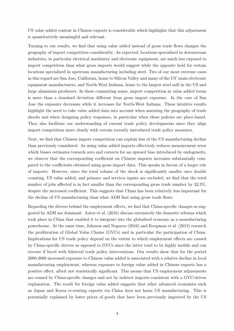
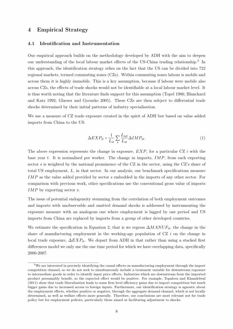
In Figure 1 we present a side-by-side comparison of the value of imports based on the industryof the imported good, i.e. a gross trade perspective, with the imported value added by industry.Given the focus of the literature on the decline of manufacturing industries in the US, we focushere on manufacturing goods and the manufacturing value added, so while embedded primarycommodities and services value added is included in the first panel, these industries are not shownin the second panel, albeit they are also indirectly exposed. As expected, we observe that theimported value added is significantly less than the gross import value for some industries such asTextiles (4), Leather and Footwear (5), Machinery (13), Electrical and Optical Equipment (14),

9

and other Manufacturing and Recycling (16). The most dramatic difference is in the Electricaland Optical Equipment sector where in 2008 US imports from China were close to USD 130billion by import value of the goods, yet only above USD 47 billion of the value added embeddedin those goods came from the Electrical and Optical Equipment sector. This illustrates howusing gross trade statistics may give a distorted picture of labour market exposure to importcompetition. In contrast to the downstream sectors listed above, we observe that for someupstream sectors which serve more often as inputs to production, such as Pulp, Paper, Printingand Publishing (7), Coke, Refined Petroleum and Nuclear Fuel (8), Chemicals (9), and Basicand Fabricated Metal (12), the embedded value added imported is significantly greater than itsgross import counterpart. This implies that local labour markets specialised in these productsare affected more than one might expect from studying gross import data.

Figure 1: Imports and Imported Value Added by Manufacturing Industry

(a) Panel 1 (b) Panel 2

Notes: WIOD codes for manufacturing industries: 3 Food, Beverages and Tobacco; 4 Textiles and Textile Products; 5Leather, Leather and Footwear; 6 Wood and Products of Wood and Cork; 7 Pulp, Paper, Paper , Printing and Publishing;8 Coke, Refined Petroleum and Nuclear Fuel; 9 Chemicals and Chemical Products; 10 Rubber and Plastics; 11 OtherNon-Metallic Mineral; 12 Basic Metals and Fabricated Metal; 13 Machinery, Nec; 14 Electrical and Optical Equipment; 15Transport Equipment; 16 Manufacturing, Nec; Recycling.

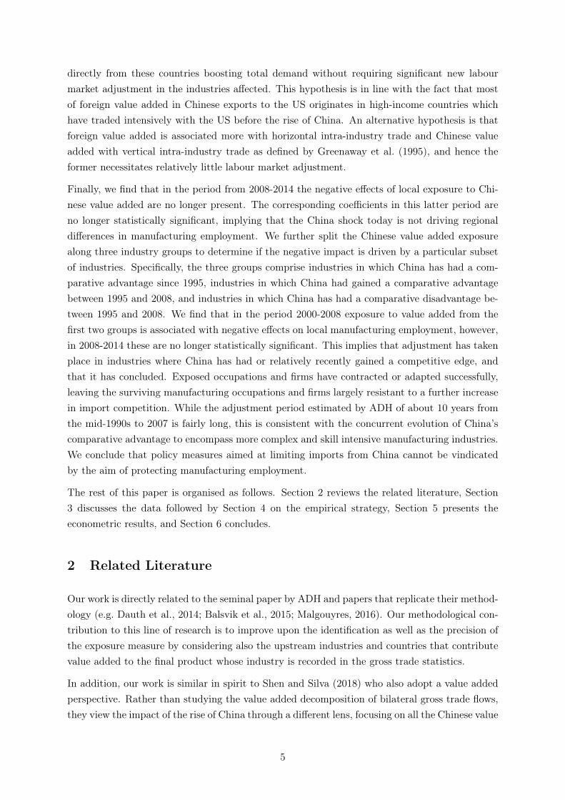
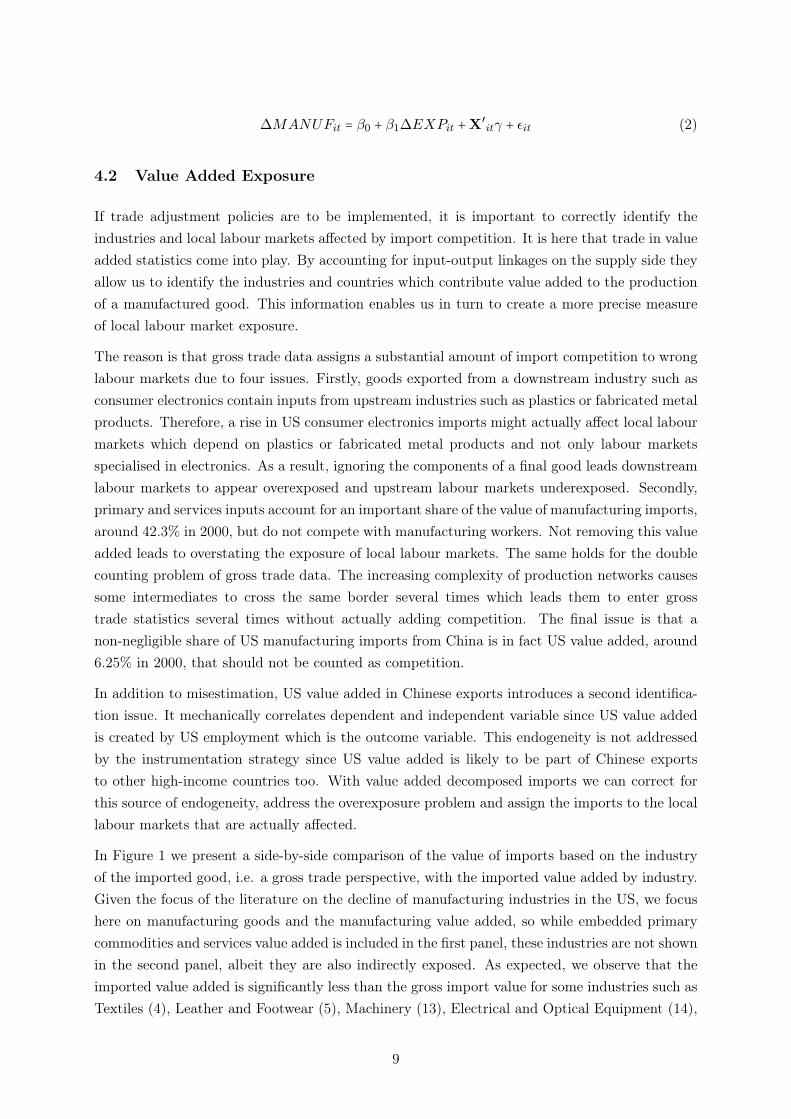
Figure 2 Illustrates that the value added content of Chinese exports to the US does not solelyoriginate from the exporting industry, but also from other upstream industries that supply inputsto the exporting industry. Different shades represent the source industries of the value addedcontent in the exports of each manufacturing industry. The industry with the largest share isusually the nominal exporting industry, however it is clear that a significant share of value added– and labour – content is contributed by other manufacturing industries, as well as primaryand services industries. It is important to note that the value added decomposition of bilateralexports does not simply take into account the direct inputs to production but also the inputs ofthese inputs, and so on.

Given these insights, we follow ADH in constructing an exposure measure based on beginning-of-period local employment in manufacturing industries, but assign import competition to labourmarkets according to which industries supplied the value added content rather than to the ex-porting industry in order to better understand the local geography of exposure to the rise of

10

Figure 2: Industry-level value added content of exports

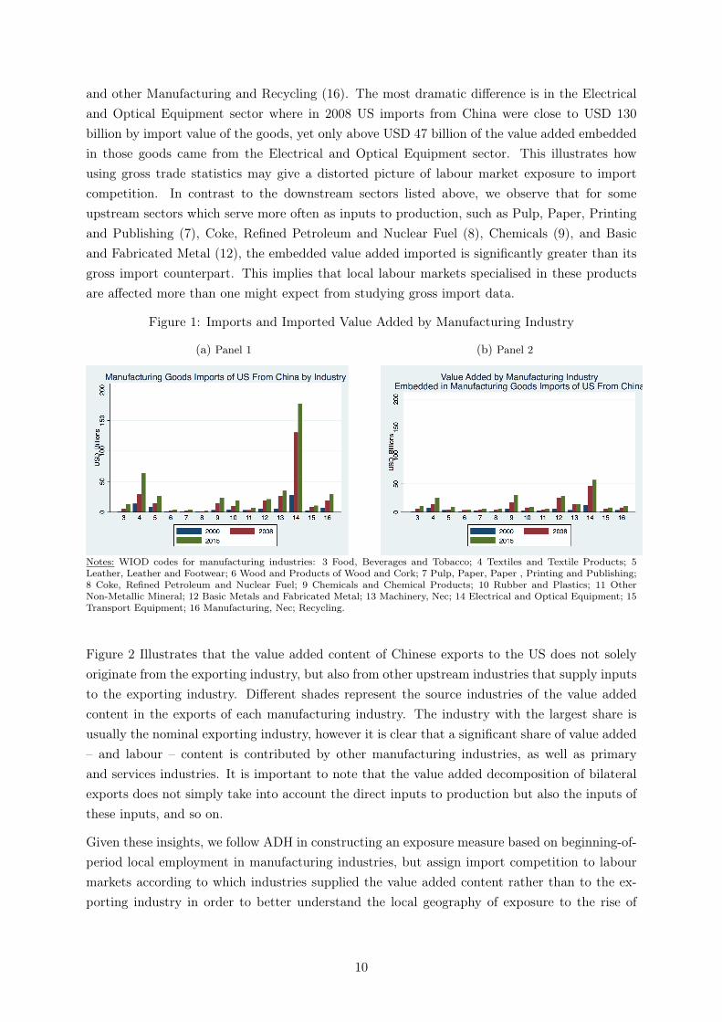
China.6 As expected and as first result, we observe that the geographic pattern differs markedlyfrom gross import based exposure measures.

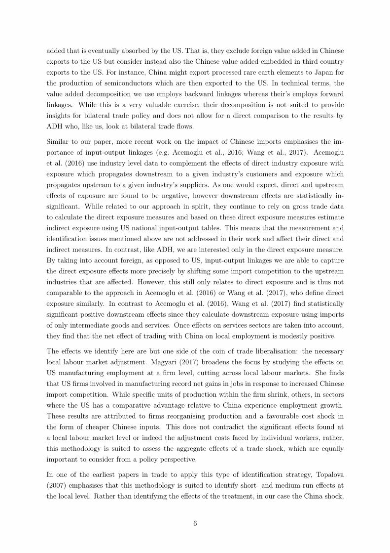
Figure 3: Difference Between Import Value and Value Added Exposure Measures

Notes: Exposure is calculated based on import growth over the 2000-2007 period. Trade data is sourced from the TiVAdatabase.

In Figure 3 we wish to highlight the differences in local labour market exposure using the twodifferent approaches. For comparability the two types of exposure are both calculated from thesame source, that is, TiVA. The colour scale in Figure 3 differentiates between below and aboveone standard deviation (of gross trade based exposure) differences between the two exposure

6Since the OECD-WTO, ADB-WIOD, and WIOD databases have been balanced so that worldwide tradeflows are mirrored, we first confirmed that the differences in the geography of exposure are not due to using adifferent dataset compared to UN Comtrade, the database used by ADH.

11

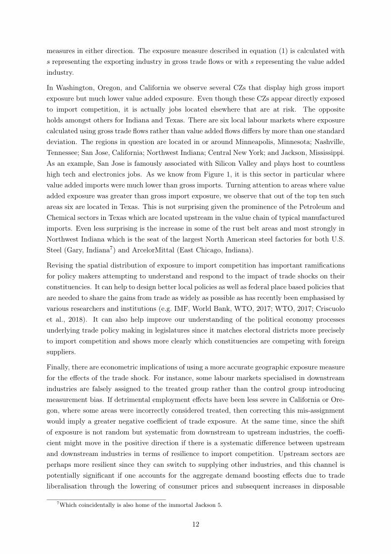
measures in either direction. The exposure measure described in equation (1) is calculated withs representing the exporting industry in gross trade flows or with s representing the value addedindustry.

In Washington, Oregon, and California we observe several CZs that display high gross importexposure but much lower value added exposure. Even though these CZs appear directly exposedto import competition, it is actually jobs located elsewhere that are at risk. The oppositeholds amongst others for Indiana and Texas. There are six local labour markets where exposurecalculated using gross trade flows rather than value added flows differs by more than one standarddeviation. The regions in question are located in or around Minneapolis, Minnesota; Nashville,Tennessee; San Jose, California; Northwest Indiana; Central New York; and Jackson, Mississippi.As an example, San Jose is famously associated with Silicon Valley and plays host to countlesshigh tech and electronics jobs. As we know from Figure 1, it is this sector in particular wherevalue added imports were much lower than gross imports. Turning attention to areas where valueadded exposure was greater than gross import exposure, we observe that out of the top ten suchareas six are located in Texas. This is not surprising given the prominence of the Petroleum andChemical sectors in Texas which are located upstream in the value chain of typical manufacturedimports. Even less surprising is the increase in some of the rust belt areas and most strongly inNorthwest Indiana which is the seat of the largest North American steel factories for both U.S.Steel (Gary, Indiana7) and ArcelorMittal (East Chicago, Indiana).

Revising the spatial distribution of exposure to import competition has important ramificationsfor policy makers attempting to understand and respond to the impact of trade shocks on theirconstituencies. It can help to design better local policies as well as federal place based policies thatare needed to share the gains from trade as widely as possible as has recently been emphasised byvarious researchers and institutions (e.g. IMF, World Bank, WTO, 2017; WTO, 2017; Criscuoloet al., 2018). It can also help improve our understanding of the political economy processesunderlying trade policy making in legislatures since it matches electoral districts more preciselyto import competition and shows more clearly which constituencies are competing with foreignsuppliers.

Finally, there are econometric implications of using a more accurate geographic exposure measurefor the effects of the trade shock. For instance, some labour markets specialised in downstreamindustries are falsely assigned to the treated group rather than the control group introducingmeasurement bias. If detrimental employment effects have been less severe in California or Ore-gon, where some areas were incorrectly considered treated, then correcting this mis-assignmentwould imply a greater negative coefficient of trade exposure. At the same time, since the shiftof exposure is not random but systematic from downstream to upstream industries, the coeffi-cient might move in the positive direction if there is a systematic difference between upstreamand downstream industries in terms of resilience to import competition. Upstream sectors areperhaps more resilient since they can switch to supplying other industries, and this channel ispotentially significant if one accounts for the aggregate demand boosting effects due to tradeliberalisation through the lowering of consumer prices and subsequent increases in disposable

7Which coincidentally is also home of the immortal Jackson 5.

12

income. We seek to answer this empirical question in the section below.

5 Econometric Results

5.1 Comparison with ADH

We are interested in the effects of trade exposure on local manufacturing employment and wefollow closely the preferred specification of ADH with the full set of controls. The dependentvariable is the change in the share of working-age population employed in manufacturing in eachCZ. Each observation is weighted by population.

∆MANUFit = β0 + β1∆EXPit +X′itγ + εit (3)

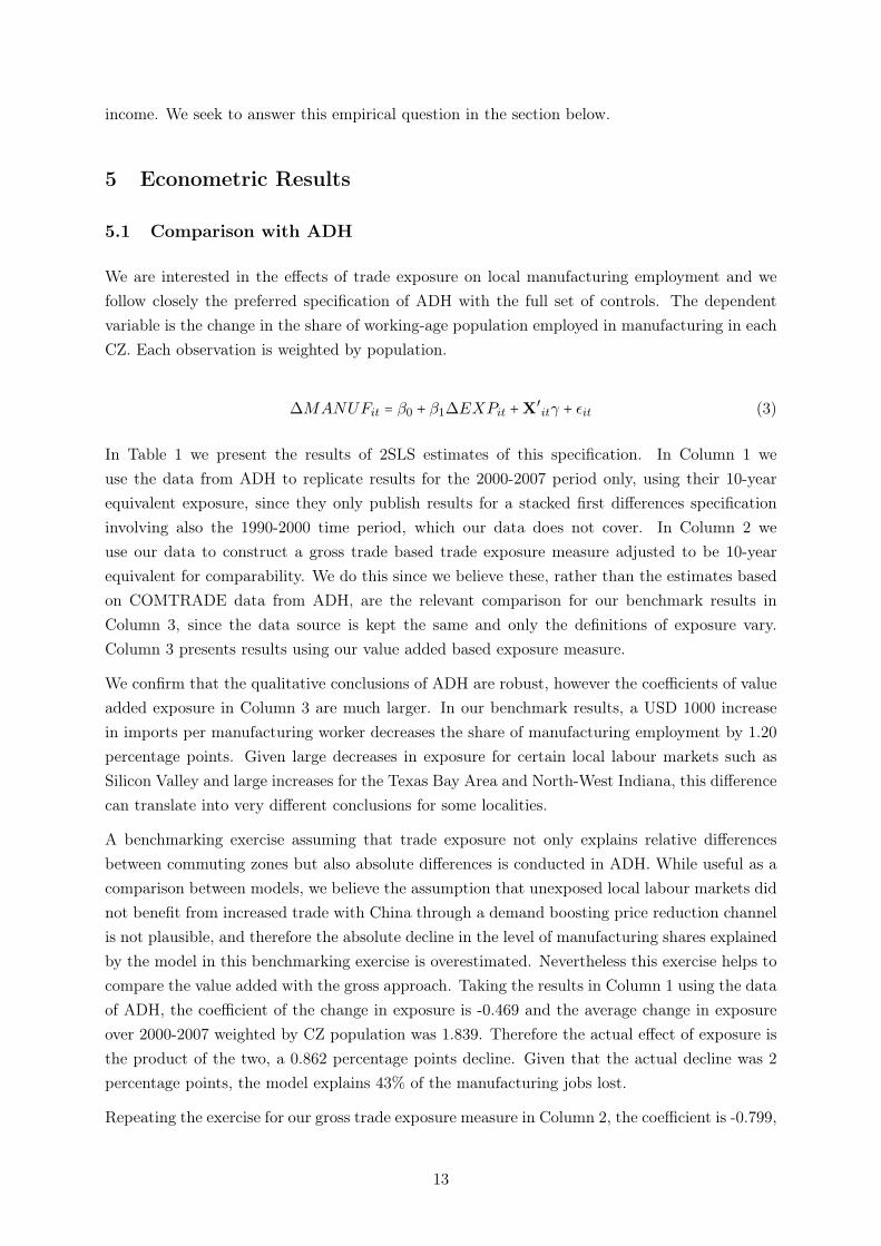
In Table 1 we present the results of 2SLS estimates of this specification. In Column 1 weuse the data from ADH to replicate results for the 2000-2007 period only, using their 10-yearequivalent exposure, since they only publish results for a stacked first differences specificationinvolving also the 1990-2000 time period, which our data does not cover. In Column 2 weuse our data to construct a gross trade based trade exposure measure adjusted to be 10-yearequivalent for comparability. We do this since we believe these, rather than the estimates basedon COMTRADE data from ADH, are the relevant comparison for our benchmark results inColumn 3, since the data source is kept the same and only the definitions of exposure vary.Column 3 presents results using our value added based exposure measure.

We confirm that the qualitative conclusions of ADH are robust, however the coefficients of valueadded exposure in Column 3 are much larger. In our benchmark results, a USD 1000 increasein imports per manufacturing worker decreases the share of manufacturing employment by 1.20percentage points. Given large decreases in exposure for certain local labour markets such asSilicon Valley and large increases for the Texas Bay Area and North-West Indiana, this differencecan translate into very different conclusions for some localities.

A benchmarking exercise assuming that trade exposure not only explains relative differencesbetween commuting zones but also absolute differences is conducted in ADH. While useful as acomparison between models, we believe the assumption that unexposed local labour markets didnot benefit from increased trade with China through a demand boosting price reduction channelis not plausible, and therefore the absolute decline in the level of manufacturing shares explainedby the model in this benchmarking exercise is overestimated. Nevertheless this exercise helps tocompare the value added with the gross approach. Taking the results in Column 1 using the dataof ADH, the coefficient of the change in exposure is -0.469 and the average change in exposureover 2000-2007 weighted by CZ population was 1.839. Therefore the actual effect of exposure isthe product of the two, a 0.862 percentage points decline. Given that the actual decline was 2percentage points, the model explains 43% of the manufacturing jobs lost.

Repeating the exercise for our gross trade exposure measure in Column 2, the coefficient is -0.799,

13

but the average change in exposure over 2000-2007 weighted by CZ population was only 1.50,and therefore the effect of exposure was -1.20 percentage points, or 59.8% of manufacturing jobslost. Using our value added based exposure measure in Column 3, the coefficient of exposureis -1.202 while the average change in exposure over 2000-2007 weighted by CZ population was0.75, yielding an effect of exposure of -0.903 percentage points or 45.2% of manufacturing jobslost.8 Since the relevant comparison in terms of data consistency is between Columns 2 and 3,we find that using gross trade exposure overstates by 32.3% the share of jobs lost which can beattributed the the trade shock under these strong assumptions.

Table 1 — A Comparison of Local Labour Market Exposure MeasuresDependent Variable: 10-year equivalent change in manufacturing employment / working-age population in % pts

(1) (2) (3)

Local exposure to Chinese exports / worker -0.469*** -0.799*** -1.202***(0.123) (0.147) (0.295)

% manufacturing employment t-1 -0.083*** -0.129*** -0.163***(0.025) (0.0305) (0.0279)

% college educated population t-1 -0.000 0.00122 -0.0102(0.021) (0.0228) (0.0237)

% foreign born t-1 0.057*** -0.00728 -0.00968(0.013) (0.0233) (0.0244)

% employment among women t-1 -0.064 0.0221 0.0268(0.039) (0.0438) (0.0470)

% employment in routine occupations t-1 -0.142 -0.248*** -0.228***(0.093) (0.0655) (0.0820)

avg offshorability of occupations t-1 -0.670* -0.154 -0.508(0.344) (0.478) (0.579)

Constant -1.182 6.528* 6.166(3.270) (3.590) (4.112)

Observations 722 722 722R-squared 0.532 0.651 0.632Census division dummies YES YES YES

2SLS first stage estimatesInstrumental Variable 0.528*** 0.755*** 0.740***

(0.0965) (0.0326) (0.0321)Adjusted R-squared 0.517 0.905 0.928Robust F 29.2963 527.251 521.698Robust standard errors in parentheses*** p<0.01, ** p<0.05, * p<0.1

5.2 Trade flows decomposed

Beyond improving the accuracy of the exposure measure, our data also allows us to distinguishbetween the true origins of the value added embedded in Chinese exports to the US. Given theremarkable expansion of Global Value Chains in the 1990s and 2000s this is relevant because itenables us to test whether the labour market effects of Chinese imports are driven by factors

8If we were to consider only the exogenous supply-driven component of exposure, a simple variance decompo-sition that uses the relationship between OLS and 2SLS estimates would indicate that its effects are only abouthalf of this.

14

specific to China, such as domestic productivity-enhancing reforms, or whether they are due tothird countries gaining competitiveness by using China as assembly hub. This has importantimplications for bilateral trade policy because in the latter case China could easily be replacedby alternative low-cost countries if bilateral trade policy barriers were to be erected while in theformer case relocation would imply losing access to a China-specific productivity multiplier.

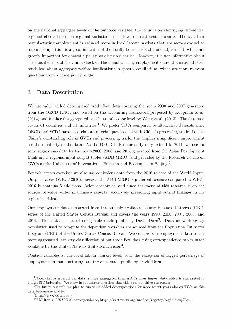
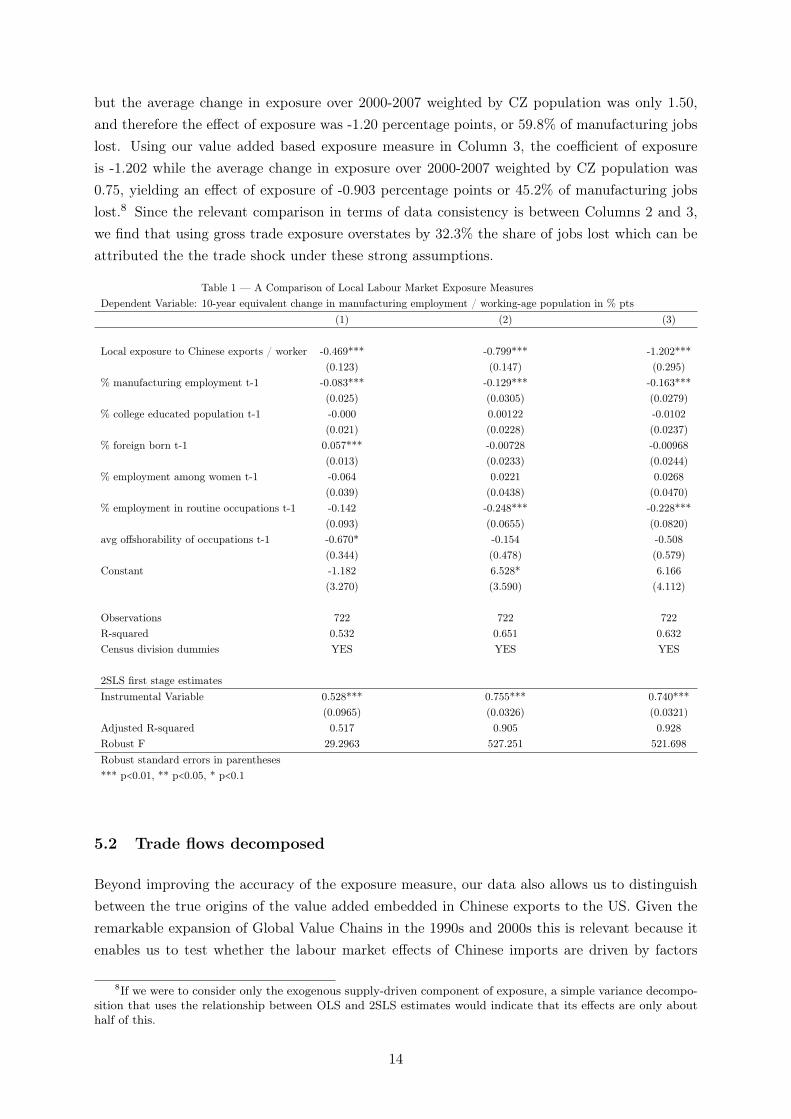
Therefore, we separate US imports from China into DVA, representing Chinese domestic valueadded, and FVA, representing foreign third-country value added, with US value added stillexcluded. Figure 4 presents two maps contrasting the geographic distribution of DVA and FVA.The specification used in this section is described in equation (4).

∆MANUFit = b0 + b1∆DV AEXPit + b2∆FV AEXPit +X′itb3 + eit (4)

In order to separately identify the causal effects of these two treatment variables on manufac-turing employment, it is a prerequisite that the industry compositions of DVA and FVA aresufficiently different. We can confirm from Figure 4 that the geographic pattern of these twoexposures indeed varies and allows for an identification. Even though DVA exposure is generallygreater in magnitude, we see important heterogeneity across industries. What stands out is thatdownstream industries, in particular electrical machinery and electronic equipment, contain ahigh share of foreign value added (72% FVA in 2000) while upstream industries such as the basicmetals industry (e.g. steel) contain predominantly Chinese value added (28% FVA in 2000). Thereason for this variation in the industry composition of DVA and FVA is an interesting topic ofresearch in its own right. This could be attributed to comparative advantage stemming from thevarying resource endowments of China and FVA contributors, China moving up the value chainas its economy develops, or a combination of factors.

Figure 4: Comparison of DVA and FVA exposure 2000-2007

(a) DVA exposure (b) FVA exposure

Notes: DVA represents Chinese domestic value added in US imports from China, FVA represents foreign third-country valueadded with US value added excluded. Exposure is calculated based on import growth over the 2000-2007 period. Tradedata is sourced from the TiVA database.

15

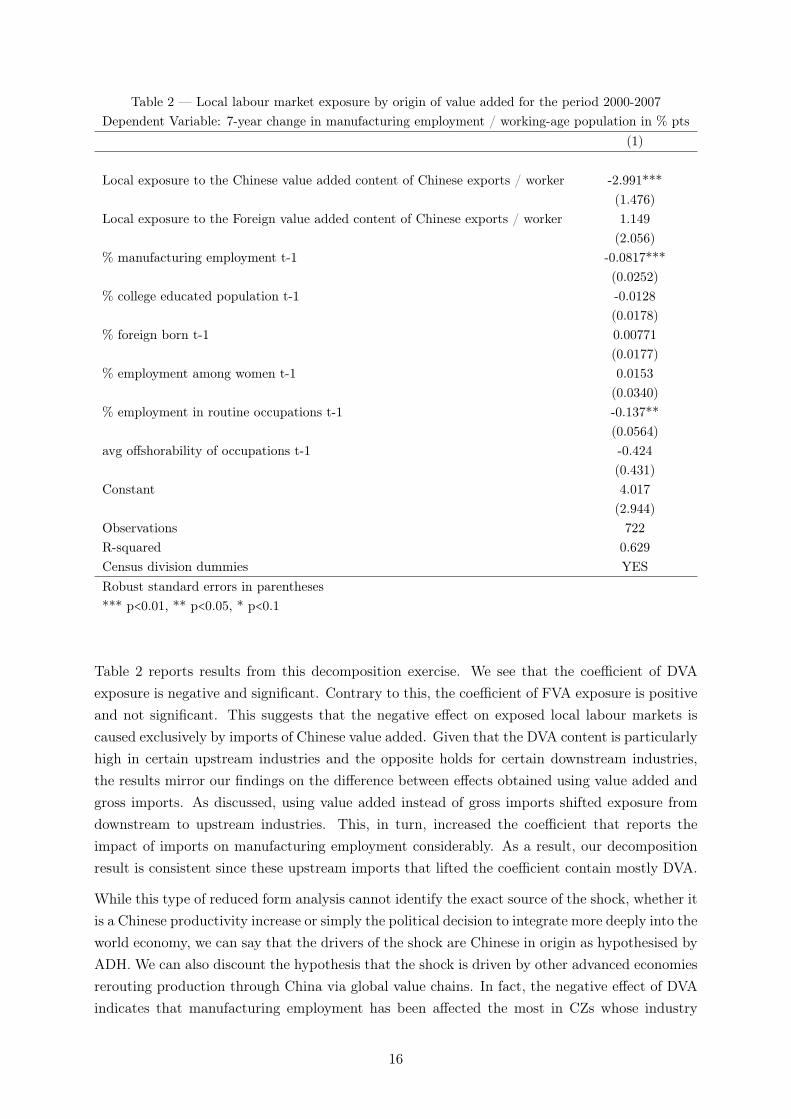
Table 2 — Local labour market exposure by origin of value added for the period 2000-2007Dependent Variable: 7-year change in manufacturing employment / working-age population in % pts

(1)

Local exposure to the Chinese value added content of Chinese exports / worker -2.991***(1.476)

Local exposure to the Foreign value added content of Chinese exports / worker 1.149(2.056)

% manufacturing employment t-1 -0.0817***(0.0252)

% college educated population t-1 -0.0128(0.0178)

% foreign born t-1 0.00771(0.0177)

% employment among women t-1 0.0153(0.0340)

% employment in routine occupations t-1 -0.137**(0.0564)

avg offshorability of occupations t-1 -0.424(0.431)

Constant 4.017(2.944)

Observations 722R-squared 0.629Census division dummies YESRobust standard errors in parentheses*** p<0.01, ** p<0.05, * p<0.1

Table 2 reports results from this decomposition exercise. We see that the coefficient of DVAexposure is negative and significant. Contrary to this, the coefficient of FVA exposure is positiveand not significant. This suggests that the negative effect on exposed local labour markets iscaused exclusively by imports of Chinese value added. Given that the DVA content is particularlyhigh in certain upstream industries and the opposite holds for certain downstream industries,the results mirror our findings on the difference between effects obtained using value added andgross imports. As discussed, using value added instead of gross imports shifted exposure fromdownstream to upstream industries. This, in turn, increased the coefficient that reports theimpact of imports on manufacturing employment considerably. As a result, our decompositionresult is consistent since these upstream imports that lifted the coefficient contain mostly DVA.

While this type of reduced form analysis cannot identify the exact source of the shock, whether itis a Chinese productivity increase or simply the political decision to integrate more deeply into theworld economy, we can say that the drivers of the shock are Chinese in origin as hypothesised byADH. We can also discount the hypothesis that the shock is driven by other advanced economiesrerouting production through China via global value chains. In fact, the negative effect of DVAindicates that manufacturing employment has been affected the most in CZs whose industry

16

structure corresponds to industries in which Chinese value added has expanded, highlighting adegree of substitutability. In contrast, manufacturing employment was unaffected in CZs whoseindustry structure mirrors the industry composition of increased FVA. This could indicate abroad shift across developed countries to expand manufacturing sectors where they maintain acomparative advantage over China in response to increased import competition in other sectors.It is also the case that the FVA component does not necessitate new adjustment as countriessuch as the US have been exposed to imports from countries such as Japan and Korea for along time. Moreover, if we sum up the total value added that key exporters send to the US,independent of the exact route these exports take, that is, independent whether they travel tothe US directly or via third countries such as China, we observe in the data that the expansionof Japanese, German, or Korean exports to the US via China comes at the expense of directexports. This means that there is no FVA import shock but simply a re-routing that does notaffect the growth rate of total imported value added from these countries. DVA on the otherhand expanded dramatically causing the observed response.

5.3 Extending the analysis until 2014

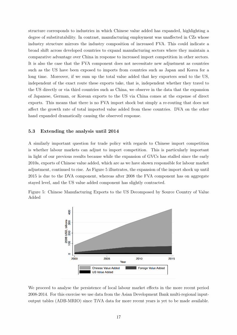
A similarly important question for trade policy with regards to Chinese import competitionis whether labour markets can adjust to import competition. This is particularly importantin light of our previous results because while the expansion of GVCs has stalled since the early2010s, exports of Chinese value added, which are as we have shown responsible for labour marketadjustment, continued to rise. As Figure 5 illustrates, the expansion of the import shock up until2015 is due to the DVA component, whereas after 2008 the FVA component has on aggregatestayed level, and the US value added component has slightly contracted.

Figure 5: Chinese Manufacturing Exports to the US Decomposed by Source Country of ValueAdded

We proceed to analyse the persistence of local labour market effects in the more recent period2008-2014. For this exercise we use data from the Asian Development Bank multi-regional input-output tables (ADB-MRIO) since TiVA data for more recent years is yet to be made available.

17

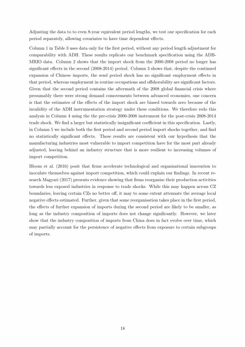
Adjusting the data to to even 8-year equivalent period lengths, we test our specification for eachperiod separately, allowing covariates to have time dependent effects.

Column 1 in Table 3 uses data only for the first period, without any period length adjustment forcomparability with ADH. These results replicate our benchmark specification using the ADB-MRIO data. Column 2 shows that the import shock from the 2000-2008 period no longer hassignificant effects in the second (2008-2014) period. Column 3 shows that, despite the continuedexpansion of Chinese imports, the send period shock has no significant employment effects inthat period, whereas employment in routine occupations and offshorability are significant factors.Given that the second period contains the aftermath of the 2008 global financial crisis wherepresumably there were strong demand comovements between advanced economies, one concernis that the estimates of the effects of the import shock are biased towards zero because of theinvalidity of the ADH instrumentation strategy under these conditions. We therefore redo thisanalysis in Column 4 using the the pre-crisis 2000-2008 instrument for the post-crisis 2008-2014trade shock. We find a larger but statistically insignificant coefficient in this specification. Lastly,in Column 5 we include both the first period and second period import shocks together, and findno statistically significant effects. These results are consistent with our hypothesis that themanufacturing industries most vulnerable to import competition have for the most part alreadyadjusted, leaving behind an industry structure that is more resilient to increasing volumes ofimport competition.

Bloom et al. (2016) posit that firms accelerate technological and organisational innovation toinoculate themselves against import competition, which could explain our findings. In recent re-search Magyari (2017) presents evidence showing that firms reorganise their production activitiestowards less exposed industries in response to trade shocks. While this may happen across CZboundaries, leaving certain CZs no better off, it may to some extent attenuate the average localnegative effects estimated. Further, given that some reorganisation takes place in the first period,the effects of further expansion of imports during the second period are likely to be smaller, aslong as the industry composition of imports does not change significantly. However, we latershow that the industry composition of imports from China does in fact evolve over time, whichmay partially account for the persistence of negative effects from exposure to certain subgroupsof imports.

18

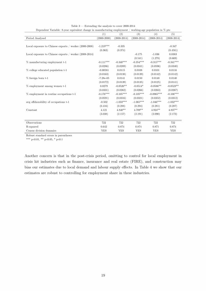
Table 3 — Extending the analysis to cover 2000-2014Dependent Variable: 8-year equivalent change in manufacturing employment / working-age population in % pts

(1) (2) (3) (4) (5)Period Analysed (2000-2008) (2008-2014) (2008-2014) (2008-2014) (2008-2014)

Local exposure to Chinese exports / worker (2000-2008) -1.219*** -0.335 -0.347(0.363) (0.374) (0.458))

Local exposure to Chinese exports / worker (2008-2014) -0.175 -1.036 0.0383(0.541) (1.278) (0.669)

% manufacturing employment t-1 -0.111*** -0.340*** -0.354*** -0.315*** -0.341***(0.0286) (0.0289) (0.0341) (0.0596) (0.0340)

% college educated population t-1 -0.00581 0.0115 0.0108 0.0101 0.0116(0.0163) (0.0138) (0.0139) (0.0142) (0.0142)

% foreign born t-1 -7.28e-05 0.0141 0.0150 0.0148 0.0140(0.0172) (0.0139) (0.0135) (0.0125) (0.0141)

% employment among women t-1 0.0279 -0.0526** -0.0514* -0.0586** -0.0523**(0.0331) (0.0262) (0.0266) (0.0263) (0.0267)

% employment in routine occupations t-1 -0.176*** -0.105*** -0.105*** -0.0965*** -0.106***(0.0591) (0.0316) (0.0321) (0.0352) (0.0312)

avg offshorability of occupations t-1 -0.502 -1.033*** -1.065*** -1.046*** -1.032***(0.416) (0.288) (0.294) (0.281) (0.287)

Constant 4.121 4.840** 4.709** 4.924** 4.837**(3.038) (2.157) (2.191) (2.090) (2.173)

Observations 722 722 722 722 722R-squared 0.642 0.874 0.874 0.871 0.874Census division dummies YES YES YES YES YES

Robust standard errors in parentheses*** p<0.01, ** p<0.05, * p<0.1

Another concern is that in the post-crisis period, omitting to control for local employment incrisis hit industries such as finance, insurance and real estate (FIRE), and construction maybias our estimates due to local demand and labour supply effects. In Table 4 we show that ourestimates are robust to controlling for employment share in these industries.

19

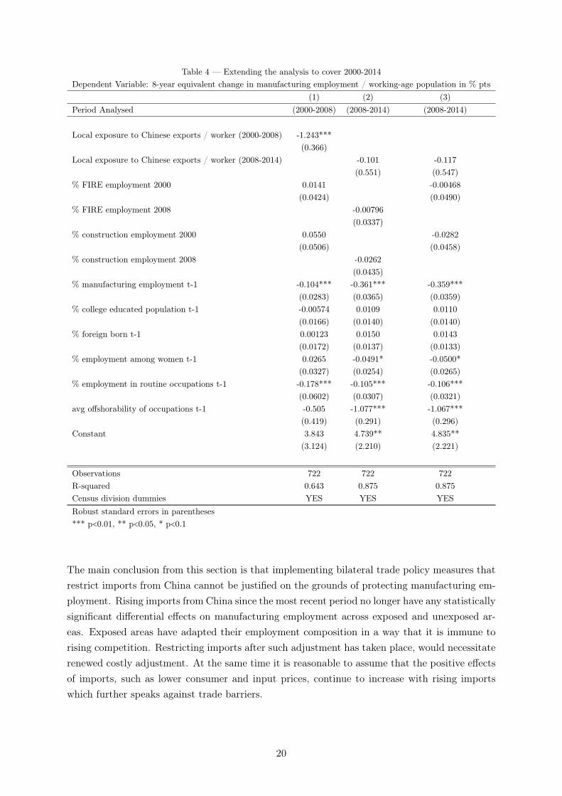
Table 4 — Extending the analysis to cover 2000-2014Dependent Variable: 8-year equivalent change in manufacturing employment / working-age population in % pts

(1) (2) (3)Period Analysed (2000-2008) (2008-2014) (2008-2014)

Local exposure to Chinese exports / worker (2000-2008) -1.243***(0.366)

Local exposure to Chinese exports / worker (2008-2014) -0.101 -0.117(0.551) (0.547)

% FIRE employment 2000 0.0141 -0.00468(0.0424) (0.0490)

% FIRE employment 2008 -0.00796(0.0337)

% construction employment 2000 0.0550 -0.0282(0.0506) (0.0458)

% construction employment 2008 -0.0262(0.0435)

% manufacturing employment t-1 -0.104*** -0.361*** -0.359***(0.0283) (0.0365) (0.0359)

% college educated population t-1 -0.00574 0.0109 0.0110(0.0166) (0.0140) (0.0140)

% foreign born t-1 0.00123 0.0150 0.0143(0.0172) (0.0137) (0.0133)

% employment among women t-1 0.0265 -0.0491* -0.0500*(0.0327) (0.0254) (0.0265)

% employment in routine occupations t-1 -0.178*** -0.105*** -0.106***(0.0602) (0.0307) (0.0321)

avg offshorability of occupations t-1 -0.505 -1.077*** -1.067***(0.419) (0.291) (0.296)

Constant 3.843 4.739** 4.835**(3.124) (2.210) (2.221)

Observations 722 722 722R-squared 0.643 0.875 0.875Census division dummies YES YES YESRobust standard errors in parentheses*** p<0.01, ** p<0.05, * p<0.1

The main conclusion from this section is that implementing bilateral trade policy measures thatrestrict imports from China cannot be justified on the grounds of protecting manufacturing em-ployment. Rising imports from China since the most recent period no longer have any statisticallysignificant differential effects on manufacturing employment across exposed and unexposed ar-eas. Exposed areas have adapted their employment composition in a way that it is immune torising competition. Restricting imports after such adjustment has taken place, would necessitaterenewed costly adjustment. At the same time it is reasonable to assume that the positive effectsof imports, such as lower consumer and input prices, continue to increase with rising importswhich further speaks against trade barriers.

20

5.4 Comparative advantage sectors

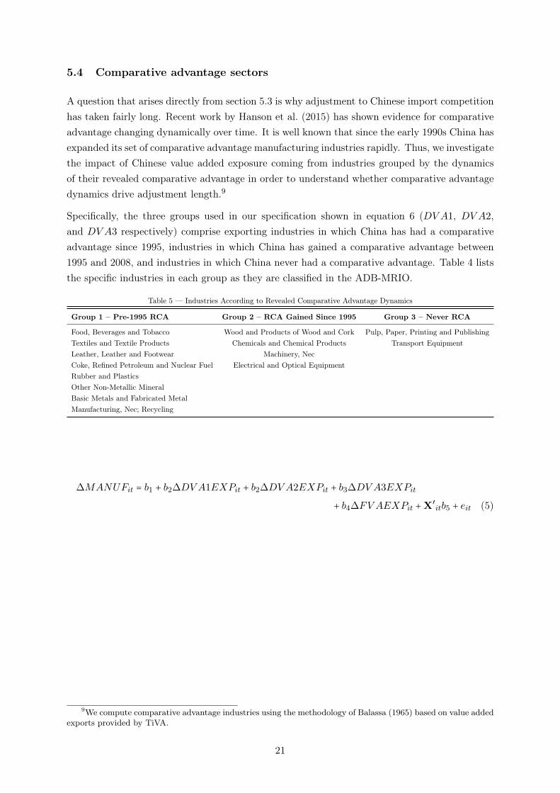
A question that arises directly from section 5.3 is why adjustment to Chinese import competitionhas taken fairly long. Recent work by Hanson et al. (2015) has shown evidence for comparativeadvantage changing dynamically over time. It is well known that since the early 1990s China hasexpanded its set of comparative advantage manufacturing industries rapidly. Thus, we investigatethe impact of Chinese value added exposure coming from industries grouped by the dynamicsof their revealed comparative advantage in order to understand whether comparative advantagedynamics drive adjustment length.9

Specifically, the three groups used in our specification shown in equation 6 (DV A1, DV A2,and DV A3 respectively) comprise exporting industries in which China has had a comparativeadvantage since 1995, industries in which China has gained a comparative advantage between1995 and 2008, and industries in which China never had a comparative advantage. Table 4 liststhe specific industries in each group as they are classified in the ADB-MRIO.

Table 5 — Industries According to Revealed Comparative Advantage Dynamics

Group 1 – Pre-1995 RCA Group 2 – RCA Gained Since 1995 Group 3 – Never RCA

Food, Beverages and Tobacco Wood and Products of Wood and Cork Pulp, Paper, Printing and PublishingTextiles and Textile Products Chemicals and Chemical Products Transport EquipmentLeather, Leather and Footwear Machinery, NecCoke, Refined Petroleum and Nuclear Fuel Electrical and Optical EquipmentRubber and PlasticsOther Non-Metallic MineralBasic Metals and Fabricated MetalManufacturing, Nec; Recycling

∆MANUFit = b1 + b2∆DV A1EXPit + b2∆DV A2EXPit + b3∆DV A3EXPit

+ b4∆FV AEXPit +X′itb5 + eit (5)

9We compute comparative advantage industries using the methodology of Balassa (1965) based on value addedexports provided by TiVA.

21

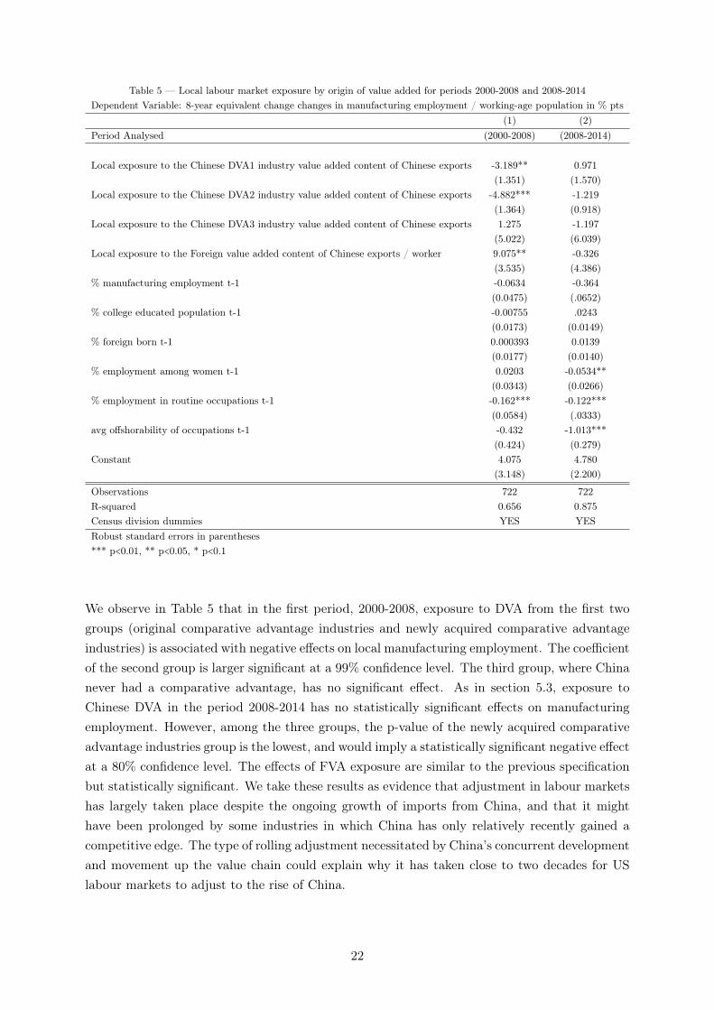
Table 5 — Local labour market exposure by origin of value added for periods 2000-2008 and 2008-2014Dependent Variable: 8-year equivalent change changes in manufacturing employment / working-age population in % pts

(1) (2)Period Analysed (2000-2008) (2008-2014)

Local exposure to the Chinese DVA1 industry value added content of Chinese exports -3.189** 0.971(1.351) (1.570)

Local exposure to the Chinese DVA2 industry value added content of Chinese exports -4.882*** -1.219(1.364) (0.918)

Local exposure to the Chinese DVA3 industry value added content of Chinese exports 1.275 -1.197(5.022) (6.039)

Local exposure to the Foreign value added content of Chinese exports / worker 9.075** -0.326(3.535) (4.386)

% manufacturing employment t-1 -0.0634 -0.364(0.0475) (.0652)

% college educated population t-1 -0.00755 .0243(0.0173) (0.0149)

% foreign born t-1 0.000393 0.0139(0.0177) (0.0140)

% employment among women t-1 0.0203 -0.0534**(0.0343) (0.0266)

% employment in routine occupations t-1 -0.162*** -0.122***(0.0584) (.0333)

avg offshorability of occupations t-1 -0.432 -1.013***(0.424) (0.279)

Constant 4.075 4.780(3.148) (2.200)

Observations 722 722R-squared 0.656 0.875Census division dummies YES YESRobust standard errors in parentheses*** p<0.01, ** p<0.05, * p<0.1

We observe in Table 5 that in the first period, 2000-2008, exposure to DVA from the first twogroups (original comparative advantage industries and newly acquired comparative advantageindustries) is associated with negative effects on local manufacturing employment. The coefficientof the second group is larger significant at a 99% confidence level. The third group, where Chinanever had a comparative advantage, has no significant effect. As in section 5.3, exposure toChinese DVA in the period 2008-2014 has no statistically significant effects on manufacturingemployment. However, among the three groups, the p-value of the newly acquired comparativeadvantage industries group is the lowest, and would imply a statistically significant negative effectat a 80% confidence level. The effects of FVA exposure are similar to the previous specificationbut statistically significant. We take these results as evidence that adjustment in labour marketshas largely taken place despite the ongoing growth of imports from China, and that it mighthave been prolonged by some industries in which China has only relatively recently gained acompetitive edge. The type of rolling adjustment necessitated by China’s concurrent developmentand movement up the value chain could explain why it has taken close to two decades for USlabour markets to adjust to the rise of China.

22

6 Conclusion

The literature on the local labour market effects of Chinese import competition has been citedextensively as an argument for limiting trade with China despite the fact that the results do notsupport this conclusion. While the differential effects of trade at a local labour market level areclear, its aggregate negative effects on manufacturing employment are subject to debate.

In this paper we provide explicit evidence that even if policy were narrowly focused on directimport competition effects ignoring price and indirect effects, there is no case for limiting tradewith China. Using recent trade data, we show that rising US local labour market exposure toChinese imports in the recent period 2008-2014 no longer has a statistically significant effect onthe relative shares of manufacturing employment. This suggests that US local labour marketadjustment to the China shock has largely concluded.

While bilateral trade barriers cannot be justified on empirical grounds, the rationale for adjust-ment policies to trade remains. Such adjustment policies require a precise understanding aboutwhich industries and regions are most affected by import competition. By exploiting a valueadded decomposition of trade flows, we improve on the accuracy of gross trade based measuresof import exposure. We find that using gross trade exposure, as done by ADH and much ofthe recent literature, overstates the direct impact of Chinese imports on US manufacturing jobsby 32.3% over the 2000-2007 period. These differences are partly because the volume of thetrade shock is smaller once only value added from manufacturing industries is considered, andpartly because the geographical distribution of import exposure is different. Using our value-added-based exposure measure changes the spatial distribution of import exposure markedly withimportant implications for interventions to facilitate adjustment and political economy analyses.Moreover, the decomposition allows us to contribute an important methodological innovationthat complements the empirical strategy of ADH with a cleaner identification of the causal ef-fects of import exposure by removing US valued added from Chinese exports to the US, whichconstitutes a mechanically endogenous component.

Finally, this paper adds to our understanding of the drivers behind the rise of China. By splittingChinese exports into a Chinese part and a part of third country inputs into Chinese production,we provide evidence that confirms the hypothesis of Autor et al. (2016) that the local labourmarket effects are driven by changes specific to China rather than the proliferation of GVCswhich have increasingly incorporated China in downstream production stages.

We find it important to emphasise and to make clear that while the focus of this line of researchhas so far been on the effects of import competition which necessitates labour market adjustmentin the short run, there are other channels in general equilibrium through which bilateral traderelations with China have welfare improving effects, and an evaluation of policy should take intoaccount both sides of the coin. While the China shock was a unique historical event, we can expectthe labour market to be affected by disruptive technology shocks in the future, and therefore,the lessons from the China shock and its impact in different countries could potentially informthe debate about optimal domestic labour market policies aimed at facilitating adjustment.

23

References

Acemoglu, Daron, David Autor, David Dorn, Gordon H Hanson, and Brendan Price,“Import competition and the great US employment sag of the 2000s,” Journal of Labor Eco-nomics, 2016, 34 (S1), S141–S198.

Adda, Jérôme and Yarine Fawaz, “The Health Toll of Import Competition,” mimeo, BocconiUniversity 2017.

Amiti, Mary, Mi Dai, Robert Feenstra, and John Romalis, “How Did China’s WTO En-try Benefit U.S. Consumers?,” Discussion Paper 12076, Centre for Economic Policy Research,London 2017.

Austin, Benjamin, Edward Glaeser, and Lawrence H Summers, “Saving the heartland:Place-based policies in 21st century America,” in “Brookings Papers on Economic Activity,Conference Draft. Washington, DC: Brookings Institution. March” 2018.

Autor, David H., David Dorn, and Gordon H. Hanson, “The China Syndrome: Local La-bor Market Effects of Import Competition in the United States,” American Economic Review,October 2013, 103 (6), 2121–68.

, , and , “The China Shock: Learning from Labor Market Adjustment to Large Changesin Trade,” Annual Review of Economics, 2016, 8, 205–240.

, , and , “When Work Disappears: Manufacturing Decline and the Falling Marriage-Market Value of Young Men,” American Economic Review: Insights, forthcoming.

, , , and Kaveh Majlesi, “A Note on the Effect of Rising Trade Exposure on the 2016Presidential Election,” mimeo, University of Zürich 2017.

Balassa, Bela, “Trade Liberalisation and “Revealed" Comparative Advantage,” The ManchesterSchool, 1965, 33 (2), 99–123.

Balsvik, Ragnhild, Sissel Jensen, and Kjell G. Salvanes, “Made in China, sold in Norway:Local labor market effects of an import shock,” Journal of Public Economics, 2015, 127, 137–144.

Blanchard, Olivier and Lawrence Katz, “Regional Evolutions,” Brookings Papers on Eco-nomic Activity, 1992, 23 (1), 1–76.

Bloom, Nicholas, Mirko Draca, and John Van Reenen, “Trade Induced Technical Change?The Impact of Chinese Imports on Innovation, IT and Productivity,” Review of EconomicStudies, 2016, 83 (1), 87–117.

Caliendo, Lorenzo, Maximiliano Dvorkin, and Fernando Parro, “The Impact of Tradeon Labor Market Dynamics,” NBER Working Papers 21149, National Bureau of EconomicResearch, Inc May 2015.

Colantone, Italo and Piero Stanig, “Global Competition and Brexit,” BAFFI CAREFINWorking Papers 1644, Universita’ Bocconi, Milano 2016.

24

Criscuolo, Chiara, Ralf Martin, Henry G. Overman, and John Van Reenen, “SomeCausal Effects of an Industrial Policy,” American Economic Review, 2018, Forthcoming.

Dauth, Wolfgang, Sebastian Findeisen, and Jens Suedekum, “The rise of the East andthe Far East: German labor markets and trade integration,” Journal of the European EconomicAssociation, 2014, 12 (6), 1643–1675.

Donoso, Vicente, Víctor Martín, and Asier Minondo, “Do differences in the exposure toChinese imports lead to differences in local labour market outcomes? An analysis for Spanishprovinces,” Regional Studies, 2015, 49 (10), 1746–1764.

Feenstra, Robert C and David E Weinstein, “Globalization, markups, and US welfare,”Journal of Political Economy, 2017, 125 (4), 1040–1074.

Glaeser, Edward L and Joseph Gyourko, “Urban Decline and Durable Housing,” The Jour-nal of Political Economy, 2005, 113 (2), 345–000.

Greenaway, David, Robert Hine, and Chris Milner, “Vertical and horizontal intra-industrytrade: a cross industry analysis for the United Kingdom,” The Economic Journal, 1995,pp. 1505–1518.

Hanson, Gordon H, Nelson Lind, and Marc-Andreas Muendler, “The dynamics of com-parative advantage,” NBER Working Papers 21753, National Bureau of Economic Research,Inc 2015.

IMF, World Bank, WTO, “Making trade an engine of growth for all : the case for trade andfor policies to facilitate adjustment,” Technical Report, International Monetary Fund, WorldBank, World Trade Organization, Geneva and Washington D.C. 2017.

Impullitti, Giammario and Omar Licandro, “Trade, firm selection and innovation: Thecompetition channel,” The Economic Journal, 2018, 128 (608), 189–229.

Johnson, Robert C. and Guillermo Noguera, “Accounting for intermediates: Productionsharing and trade in value added,” Journal of International Economics, 2012, 86 (2), 224–236.

and , “A Portrait of Trade in Value Added over Four Decades,” NBER Working Papers22974, National Bureau of Economic Research, Inc 2016.

Koopman, Robert, Zhi Wang, and Shang-Jin Wei, “Estimating domestic content in ex-ports when processing trade is pervasive,” Journal of Development Economics, 2012, 99 (1),178–189.

, , and , “Tracing value-added and double counting in gross exports,” The AmericanEconomic Review, 2014, 104 (2), 459–494.

Magyari, Ildiko, “Firm Reorganization, Chinese Imports, and US Manufacturing Employ-ment,” mimeo, Colombia University 2017.

Malgouyres, Clément, “The impact of Chinese import competition on the local structure ofemployment and wages: Evidence from France,” Journal of Regional Science, 2016, forthcom-ing.

25

Shen, Leilei and Peri Silva, “Value-added exports and US local labor markets: Does Chinareally matter?,” European Economic Review, 2018, 101, 479–504.

Topalova, Petia, “Trade liberalization, poverty and inequality: Evidence from Indian districts,”in Ann Harrison, ed., Globalization and poverty, University of Chicago Press, 2007, pp. 291–336.

and Amit Khandelwal, “Trade liberalization and firm productivity: The case of India,”Review of economics and statistics, 2011, 93 (3), 995–1009.

Topel, Robert H, “Local labor markets,” Journal of Political economy, 1986, 94 (3, Part 2),S111–S143.

Wang, Zhi, Shang-Jin Wei, and Kunfu Zhu, “Quantifying international production sharingat the bilateral and sector levels,” Technical Report, National Bureau of Economic Research2013.

, , Xinding Yu, and Kunfu Zhu, “Rethinking the Impact of the China Trade Shock onthe US Labor Market: A Production-Chain Perspective,” mimeo, Colombia University 2017.

WTO, “World Trade Report 2017: Trade, technology, and jobs,” Technical Report, World TradeOrganization, Geneva 2017.

26

Appendix

The China Shock revisited: Insights from value added trade flows: Valueadded decomposition of gross trade flows at bilateral-sector level

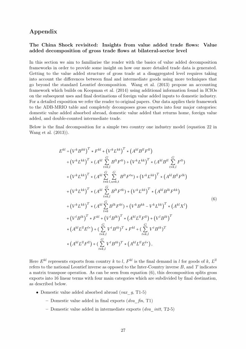
In this section we aim to familiarise the reader with the basics of value added decompositionframeworks in order to provide some insight on how our more detailed trade data is generated.Getting to the value added structure of gross trade at a disaggregated level requires takinginto account the differences between final and intermediate goods using more techniques thatgo beyond the standard Leontief decomposition. Wang et al. (2013) propose an accountingframework which builds on Koopman et al. (2014) using additional information found in ICIOson the subsequent uses and final destinations of foreign value added inputs to domestic industry.For a detailed exposition we refer the reader to original papers. Our data applies their frameworkto the ADB-MRIO table and completely decomposes gross exports into four major categories:domestic value added absorbed abroad, domestic value added that returns home, foreign valueadded, and double-counted intermediate trade.

Below is the final decomposition for a simple two country one industry model (equation 22 inWang et al. (2013)).

Ekl = (V kBkk)T ∗ F kl + (V kLkk)T ∗ (AklBllF ll)

+ (V kLkk)T ∗ (AklG

∑t≠k,l

BltF tt) + (V kLkk)T ∗ (AklBllG

∑t≠k,l

F lt)

+ (V kLkk)T ∗ (AklG

∑t≠k

G

∑l,u≠k,t

BltF tu) + (V kLkk)T ∗ (AklBllF lk)

+ (V kLkk)T ∗ (AklG

∑t≠k,l

BltF tk) + (V kLkk)T ∗ (AklBlkF kk)

+ (V kLkk)T ∗ (AklG

∑t≠k

BlkF kt) + (V kBkk − V kLkk)T ∗ (AklX l)

+ (V lBlk)T ∗ F kl + (V lBlk)T ∗ (AklLllF ll) + (V lBlk)T

∗ (AklLllEl∗) + (G

∑t≠k,l

V tBtk)T ∗ F kl + (G

∑t≠k,l

V tBtk)T

∗ (AklLllF ll) + (G

∑t≠k,l

V tBtk)T ∗ (AklLllEl∗) ,

(6)

Here Ekl represents exports from country k to l, F kl is the final demand in l for goods of k, Lll

refers to the national Leontief inverse as opposed to the Inter-Country inverse B, and T indicatesa matrix transpose operation. As can be seen from equation (6), this decomposition splits grossexports into 16 linear terms with four main categories which are subdivided by final destination,as described below.

• Domestic value added absorbed abroad (vax_g, T1-5)

– Domestic value added in final exports (dva_fin, T1)

– Domestic value added in intermediate exports (dva_intt, T2-5)

27

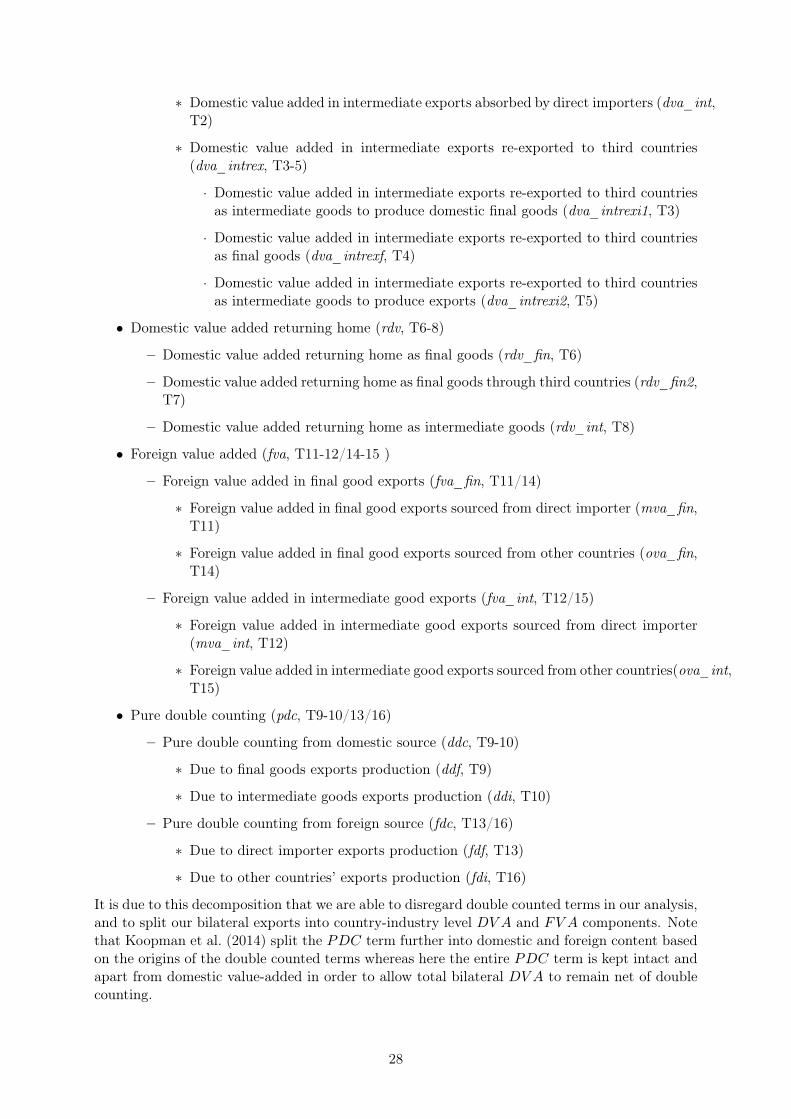
∗ Domestic value added in intermediate exports absorbed by direct importers (dva_int,T2)

∗ Domestic value added in intermediate exports re-exported to third countries(dva_intrex, T3-5)

· Domestic value added in intermediate exports re-exported to third countriesas intermediate goods to produce domestic final goods (dva_intrexi1, T3)

· Domestic value added in intermediate exports re-exported to third countriesas final goods (dva_intrexf, T4)

· Domestic value added in intermediate exports re-exported to third countriesas intermediate goods to produce exports (dva_intrexi2, T5)

• Domestic value added returning home (rdv, T6-8)

– Domestic value added returning home as final goods (rdv_fin, T6)

– Domestic value added returning home as final goods through third countries (rdv_fin2,T7)

– Domestic value added returning home as intermediate goods (rdv_int, T8)

• Foreign value added (fva, T11-12/14-15 )

– Foreign value added in final good exports (fva_fin, T11/14)

∗ Foreign value added in final good exports sourced from direct importer (mva_fin,T11)

∗ Foreign value added in final good exports sourced from other countries (ova_fin,T14)

– Foreign value added in intermediate good exports (fva_int, T12/15)

∗ Foreign value added in intermediate good exports sourced from direct importer(mva_int, T12)

∗ Foreign value added in intermediate good exports sourced from other countries(ova_int,T15)

• Pure double counting (pdc, T9-10/13/16)

– Pure double counting from domestic source (ddc, T9-10)

∗ Due to final goods exports production (ddf, T9)

∗ Due to intermediate goods exports production (ddi, T10)

– Pure double counting from foreign source (fdc, T13/16)

∗ Due to direct importer exports production (fdf, T13)

∗ Due to other countries’ exports production (fdi, T16)

It is due to this decomposition that we are able to disregard double counted terms in our analysis,and to split our bilateral exports into country-industry level DV A and FV A components. Notethat Koopman et al. (2014) split the PDC term further into domestic and foreign content basedon the origins of the double counted terms whereas here the entire PDC term is kept intact andapart from domestic value-added in order to allow total bilateral DV A to remain net of doublecounting.

28