Tail Risk and Return Predictability for the Japanese Equity Market∗

Torben G. Andersen† Viktor Todorov‡ Masato Ubukata§

May 7, 2019

Abstract

This paper studies the predictability of the Japanese equity market, focusing on the forecast-

ing power of nonparametric volatility and tail risk measures obtained from options data on

the S&P 500 and Nikkei 225 market indices. The Japanese market is notoriously difficult to

forecast using standard predictive indicators. We confirm that country-specific regressions for

Japan – contrary to existing evidence for other national equity indices – produce insignificant

predictability patterns. However, we also find that the U.S. option-implied tail risk measure

provides significant forecast power both for the dollar-yen exchange rate and the Japanese ex-

cess returns, especially when measured in U.S. dollars. Thus, the dollar-denominated Japanese

returns are, in fact, predictable through the identical mechanism as for other equity market

indices, suggesting a high degree of global integration for the Japanese financial market.

Keywords: Tail Risk, Variance Risk Premium, Option Markets, Return Predictability.

JEL classification: G12, G13, G15, G17.

∗This work is partially supported by NSF grant SES-1530748 and JSPS KAKENHI grant JP15K03397,

JP18K01690. In addition, Andersen gratefully acknowledges support from CREATES, Center for Research in Econo-

metric Analysis of Time Series (DNRF78), funded by the Danish National Research Foundation. We thank the Guest

Editor, Zhengjun Zhang, and two anonymous referees for many suggestions that significantly improved the paper.

We also thank participants at the 2nd International Conference on Econometrics and Statistics (EcoSta 2018) at City

University of Hong Kong, June 2018, the University of San Diego Conference in celebration of Tim Bollerslev’s 60’th

birthday, October 2018, and the Financial Management Association Conference on Derivatives and Volatility at the

CBOE, Chicago, November 2018, for useful comments.†Kellogg School, Northwestern University, Evanston, IL 60208; e-mail: t-andersen@northwestern.edu.‡Kellogg School, Northwestern University, Evanston, IL 60208; e-mail: v-todorov@northwestern.edu.§Department of Economics, Meiji Gakuin University, Shirokanedai, Minato-ku, Tokyo, 108-0071 Japan, e-mail:

ubukata@eco.meijigakuin.ac.jp

1 Introduction

An extensive literature suggests that a number of economic and financial variables possess forecast

power for long-horizon excess returns on the aggregate equity market. The early contributions

emphasize predictors such as the ratio of prices to dividends or earnings, see, e.g., Campbell and

Shiller (1988a,b), Fama and French (1988), and Hodrick (1992), as well as a variety of interest and

yield spread measures, see Campbell (1987), Fama and French (1989), and Keim and Stambaugh

(1986), among others. However, subsequently, a number of studies assert that methodological issues,

primarily due to the extreme persistence of the predictors and potential model misspecification,

severely distort the associated inference procedures. For example, Ang and Bekaert (2007), Welch

and Goyal (2008), Boudoukh et al. (2008), and Hjalmarsson (2011) conclude that there is no credible

evidence of long-run predictability for the U.S. aggregate market returns. Nonetheless, the topic

remains unsettled, and the hypothesis that expected excess returns—the equity risk premium—

varies over time, and in particular across the business cycle, remains widely accepted.

To assess the robustness of these findings, various authors explore the forecast power of the same

predictors for major international stock markets. As for the U.S., the predictors often generate

predictive patterns according to standard inference procedures, although the findings vary and

never provide a fully coherent picture across countries. The Japanese equity market has attracted

particular attention, as the studies typically fail to produce significant results and, more generally,

reveal features that deviate substantially from the usual pattern in other developed countries, see,

e.g., Schrimpf (2010), Aono and Iwaisako (2010, 2011, 2013), and Tsuji (2009) for recent evidence.

Meanwhile, over the past decade, a separate set of studies documents significant medium-term

predictability for stock returns based on the premium associated with exposure to equity return

variation. Specifically, Bollerslev et al. (2009) find that the variance risk premium, obtained as the

gap between the option-based risk-neutral and the statistically expected future return variation,

predicts the equity risk premium for horizons spanning four to twelve months. Not surprisingly,

this finding has also been studied extensively, including for international markets, with authors

generally confirming the positive association among the variance and equity risk premiums, albeit

with varying degrees of significance depending on the particular equity index and sample period

explored. One advantage of the variance risk premium (from a statistical point of view) is that,

relative to the extremely persistent regressors used in the long-horizon predictability studies, it

1

is substantially less persistent, generating fewer econometric problems. Nonetheless, as for the

macroeconomic and yield-based predictors, the evidence for predictability via the variance risk

premium is absent in the Japanese stock market, see, e.g., Londono (2011), Bollerslev et al. (2014),

and Ubukata and Watanabe (2014).

Finally, a number of recent studies reveal that the predictability afforded by the variance risk

premium stems largely from the left jump tail, as detailed for the U.S. market in Bollerslev et al.

(2015). Specifically, Andersen et al. (2015, 2019) document strong predictability associated with

the left tail component for both the U.S. and a set of European equity indices, while they also

find that the variance risk premium, stripped of the left tail premium, has insignificant predictive

power for all indices. These results suggest that the compensation for exposure to abrupt downside

movements in the index is at the core of the return predictability.

In this paper, we seek to establish whether the documented lack of forecast power for the

variance risk premium in Japan represents yet another fundamental difference vis-a-vis other de-

veloped economies, or whether, alternatively, the results may arise from the way equity tail risk is

compensated in the Japanese financial markets.

To achieve this goal, we follow Bollerslev and Todorov (2014) and Bollerslev et al. (2015) and

construct model-free measures of left tail variation from the option data for the U.S. and Japanese

stock market indices. The tail measures are based on extreme value theory, and to the best of our

knowledge, have not been constructed before for the Nikkei index. We document that, as for the

U.S. stock market, deep out-of-the-money log-put prices written on the Japanese market index decay

linearly as function of their log-strikes, consistent with what is implied by regular variation of the left

tail of the underlying return distribution. Our measures of tail variation on the U.S. and Japanese

markets have similarities and notable differences in their time series behavior. For example, they

both increase around the time of the financial crisis in the Fall of 2008, but the Japanese tail measure

also reacts strongly to country-specific events such as the Fukushima earthquake. The differences in

the time series behavior of the two tail measures manifest themselves in different predictive ability

for the Japanese equity risk premium. For Japan, we verify that return predictability is elusive

using traditional country-specific predictors: neither the variance risk premium nor the left tail

jump risk premium provide significant forecasts for the future Nikkei 225 index returns. On the

other hand, the U.S. tail measure shows weak predictability for the Japanese stock market returns,

2

while the results turn highly significant for the corresponding dollar-denominated returns. Thus,

from the point of view of a global investor, the predictive results for the Japanese market are similar

to these in other leading stock markets.

The remainder of this paper is structured as follows. Section 2 describes our data sources, with

an emphasis on the Japanese option data which have not been explored for this type of analysis

previously. Section 3 introduces the theoretical framework and details our estimation and implemen-

tation procedures. Section 4 presents results for predictive regressions involving the country-specific

option and financial market data. In Section 5, we adopt a global perspective, letting the U.S. left

tail jump premium serve as predictor for the yen- and dollar-denominated Japanese equity index.

Section 6 explores whether equity tail-risk compensation can also help predict future movements

in the dollar-yen exchange rate, and Section 7 provides concluding remarks. Additional results and

details regarding the empirical implementation are available in a Supplementary Appendix.

2 Data

We rely on data for the primary equity market indices in the U.S. and Japan from January 1996

to June 2018. We proxy the market portfolio in Japan with the Nikkei 225 Total Return Index

(Nikkei 225) provided by Nikkei inc., capturing the performance of the Nikkei Stock Average. It

includes changes in the index level and reinvestment of dividend income from its 225 constituent

stocks listed on the first section of the Tokyo Stock Exchange.1 Similarly, we use the S&P 500 Total

Return Index (S&P 500) to account for dividends.2 The index values, sampled at the end of each

month in Japan, are expressed both in local currency and U.S. dollars. We obtain the local excess

returns by subtracting the three-month Treasury bill rate in the U.S. and the unsecured overnight

call rate in Japan from the respective local (continuously compounded) market return. The U.S.

dollar-denominated Nikkei 225 excess returns equal the yen Nikkei 225 market returns plus the log

U.S. dollar-Japanese yen exchange rate return minus the U.S. risk-free rate.

1The TOPIX Total Return Index (cum dividends) is available from the Tokyo Stock Exchange (TSE). This

value-weighted index is based on all domestic common stocks in the first section of the TSE. Figures A.1–A.3 of the

Supplementary Appendix document that our results are qualitatively identical for the TOPIX Total Return Index.2In calculating the total return index for the S&P 500, dividends paid by the individual companies are invested

in the entire index, not just in the stock paying the dividend.

3

Descriptive statistics for the monthly return series from February 1996 to July 2017 (258

months)—corresponding to the period over which we produce forecasts regarding future returns—

are provided in Table 1.3 The mean monthly dollar- and yen-denominated excess returns for the

Japanese market are −0.10% and 0.08%, with monthly values ranging from −19.6% to 16.5% and

−27.3% to 12.2%, respectively. These figures are qualitatively similar for the U.S. index, except for

the markedly better average return of 0.50%. The monthly dollar-yen returns have relatively small

standard deviations, but the kurtosis of 5.52 is comparable to those for the market excess returns.

The estimated first-order autocorrelation of the monthly returns ranges from 0.01 for the dollar-yen

rate to 0.12 for the dollar denominated Nikkei 225 index. In Panel B, the sample cross-correlations

of the local equity-index returns versus the dollar-yen exchange rate returns are negative but, not

surprisingly, positive for the dollar-denominated Nikkei 225 index.

Next, we describe our Japanese option data in some detail, as they typically have not been

available for prior empirical studies. The Nikkei 225 index options are obtained from Nikkei NEEDS

Financial Quest 2.0, which provides closing bid and ask quotes as well as transaction prices for

options traded on the Osaka Securities Exchange. The Nikkei 225 options are European style, and

each contract trades until the business day preceding the second Friday of the expiration month (or

if the second Friday is a non-business day, the preceding business day). The final settlement price,

known in Japan as the special quotation or SQ, is calculated based on the total opening prices of

each component stock of Nikkei 225 on the business day following the last trading day. We remove

contracts with zero bid or ask quotes, and we compute the daily mid-quote as the simple average

of the bid and ask quote for each available option contract.4

Table 2 summarizes the main features of our Nikkei 225 out-of-the-money (OTM) option data

covering January 2006 to June 2017. We do not use data prior to 2006 due to the sparcity of deep

OTM options needed to estimate the implied jump risk measures. In Panel A, the OTM options are

sorted by tenor in calendar days. The average percentage bid-ask spread is the simple average of

100× (ask− bid)/ask. The average daily number of put options is about 50 versus 36 call options,

3The last observation exploited to generate return predictions is June 2017, while returns up to the end of June

2018 are used to assess forecast performance over one to twelve month horizons.4The Osaka Securities Exchange introduced options with expiry for each of the nearest four weeks beginning May

25, 2015. Without access to weekly options in Japan over our sample period, we also restrict ourselves to regular

monthly S&P 500 options for the U.S.

4

and the average bid-ask spread for puts ranges from around 13% to 17%, lower than the call range

of 15% to 19%. The available contracts are fairly evenly distributed across tenors from a few weeks

till three months. The average Black-Scholes implied volatility (BSIV) of the put contracts exceeds

those for the calls by a substantial margin at about 34% versus 23%.

In Panel B, the near- and next-term OTM options are sorted by moneyness, defined as the

ratio of the strike over forward price. These two option categories are used in the calculation

of model-free implied volatility measures at the end of each month. The near-term includes the

shortest maturity option each trading day, excluding those with less than eight days to expiration.

The average number of near- and next-term OTM options are around 29 and 37 per trading day,

respectively. The bid-ask spreads for the deep OTM options are higher than those for at-the-money

(ATM) options. The usual volatility skew in equity-index options is also present in Japan, as the

BSIV for the deep OTM put options, in particular, are much higher than for the ATM options.

Panel C provides information on the deep OTM put and call options available per week using

the moneyness definition commensurate with the construction of our nonparametric tail measures.

The OTM metric is now defined as the log-moneyness normalized by the ATM BSIV. The figures

refer to options with tenor between eight and forty-four days only, and we report on the initial part

of the sample separately to convey the growth in liquidity over time. As seen from the table, even

early in our sample, we have a considerable number of deep OTM options (volatility-standardized

log-moneyness below −2.5 for puts, above 1.5 for calls) available. Overall, this Nikkei OTM option

sample provides a good basis for the computation of the option-based jump risk measures introduced

in the following section.

3 Nonparametric Option-Based Risk Measures

3.1 Decomposing Variance Risk Premium

The generic asset price St is defined on a filtered probability space (Ω,F ,P), with (Ft)t≥0 denoting

the associated filtration. We assume St follows a stochastic exponential of a general jump-diffusion,

dSt/St− = at dt + σt dWt +

∫R

(ex − 1) µP(dx, dt), (1)

5

where the drift and diffusive processes, at and σt , are assumed to have cadlag paths, but otherwise

are left unspecified, Wt is a standard Brownian motion, x indicates the jump size of the log-price,

µP(dx, dt) ≡ µ(dx, dt) − νPt (dx)dt is a martingale measure under the actual probability measure,

P, where µ(dx, dt) counts the jumps in S, and νPt (dx) denotes the jump compensator, i.e., the

(predictable) jump intensity process under P. The return variation of the log-price process over t

to t+ τ is measured by the quadratic variation,

QVt,t+τ =

∫ t+τ

tσ2s ds +

∫ t+τ

t

∫Rx2 µ(dx, ds). (2)

We assume the existence of a risk-neutral probability measure, Q, under which the cum-dividend

discounted asset price is a local martingale.5 The P − Q wedge is due to compensation for risk,

i.e., a risk premium. In particular, the variance risk premium, normalized by the horizon, V RPt,τ ,

is given by the gap between the conditional expectations of QVt,t+τ under the risk-neutral and

objective measures, Q and P,

V RPt,τ ≡1

τ

(EQt [QVt,t+τ ]− EP

t [QVt,t+τ ]), (3)

which represents compensation for the risk associated with fluctuations in the return variation.6

The VRP provides compensation for two distinct types of risks: time-varying volatility and

jumps. Letting CVt,t+τ =∫ t+τt σ2sds be the continuous variation, and JVPt,t+τ =

∫ t+τt

∫R x

2νPs (dx)ds

and JVQt,t+τ =∫ t+τt

∫R x

2νQs (dx)ds denote the predictable jump variation under P and Q, respec-

5The existence of Q is guaranteed by no-arbitrage under standard regularity conditions, see, e.g., Duffie (2001).6The variance risk premium is usually defined, V RPt,τ ≡ EP

t [QVt,t+τ ] − EQt [QVt,t+τ ], whereas the return pre-

dictability literature often uses the expression (3), e.g., Londono (2011) and Bollerslev et al. (2014), to obtain an

(average) positive premium. Consumption-based asset pricing models incorporating time-varying economic uncer-

tainty imply a positive relationship between the equity risk premium and variance risk premium, which may serve as

a gauge of investor risk aversion; see Bollerslev et al. (2009, 2011) and Drechsler and Yaron (2011).

6

tively, we may decompose the VRP as,

V RPt,τ =1

τ

(EQt [CVt,t+τ ]− EP

t [CVt,t+τ ])

+1

τ

(EQt [JVQt,t+τ ]− EP

t [JVPt,t+τ ])

=1

τ

(EQt [CVt,t+τ ]− EP

t [CVt,t+τ ])

+1

τ

(EQt [JVPt,t+τ ]− EP

t [JVPt,t+τ ])

+1

τ

(EQt [JVQt,t+τ ]− EQ

t [JVPt,t+τ ]). (4)

The terms in the middle line of equation (4) reflect compensation for the risk associated with

variation in the diffusive volatility and jump intensity risk. They may be viewed as premiums

incurred for hedging against changes in the investment opportunity set for the aggregate market

portfolio. By contrast, the last term captures the wedge between the Q and P jump variation

under the risk-neutral measure. It signifies compensation for the possibility that jumps may occur,

as distinct from the compensation for temporal variation in the jump intensity.7 Bollerslev et al.

(2015) and Andersen et al. (2015, 2019) find that a large portion of the predictability of the U.S.

aggregate stock returns might be attributed to the compensation for this jump tail risk component.

We now introduce our jump tail risk measurement procedures for the U.S. and Japanese markets.

3.2 Estimating Implied and Expected Realized Variance and Jump Tail Risk

We start with reviewing the essentially model-free estimation procedure for the variance risk pre-

mium and its jump tail risk component. We obtain the VRP as the difference between a model-free

option-implied variance and an expected realized variance. The former approximates the risk-

neutral expectation of the quadratic variation for the market index over a fixed maturity using the

option prices for the corresponding tenor. As shown by Carr and Madan (1998), Demeterfi et al.

(1999) and Britten-Jones and Neuberger (2000), we have,

1

τEQt [QVt,t+τ ] ≈ 2 ertτ

τ

(∫ Ft,τ

0

Pt,τ(K)

K2dK +

∫ ∞Ft,τ

Ct,τ(K)

K2dK

), (5)

7See section 5 in Bollerslev and Todorov (2011) and section 2.2 in Bollerslev et al. (2015) for detailed discussion.

7

where rt is the risk-free rate, Pt,τ (K) and Ct,τ (K) are the European put and call option prices with

strike K, Ft,τ is the forward price, all at time t and with maturity date t+ τ .8

This representation constitutes the basis for well-known model-free market volatility indices,

including the VIX. We approximate the integral on the right-hand side of equation (5) using a

Riemann sum and option prices on an equidistant grid of 1, 001 strikes covering a range of three

times the standard deviation around the log forward price. Options on this grid are in turn

approximated from the available ones using cubic spline interpolation in the BSIV space. Outside

this range —beyond the smallest and highest available strikes—the BSIV level is assumed flat.

Finally, thirty (calendar) day implied measures are calculated by linear interpolation across the two

nearest maturities, excluding maturities below eight days. This approach is known to work well for

S&P 500 index options, see Carr and Wu (2009).9 Panel B of Table 2 in Section 2 characterizes

the basic features of the Japanese OTM option sample available for estimation.

For the P-conditional expectation of the quadratic variation, EPt [QVt,t+τ ], we use a realized vari-

ance forecast based on a standard time-series model. First popularized by Andersen and Bollerslev

(1998), Andersen et al. (2001) and Barndorff-Nielsen and Shephard (2002), the realized variance,

defined as the sum of the squared intraday returns over the interval, provides an accurate estimate

of the quadratic variation in the absence of microstructure noise induced by frictions such as bid-ask

bounce and non-synchronous trading. To mitigate microstructure effects, we rely on daily realized

variances obtained from five-minute returns generated by the Oxford-Man Institute Realized Li-

brary. Next, we estimate the heterogeneous autoregressive (HAR) model of Corsi (2009), using the

past 900 daily realized variances. It is a simple approximate long-memory model for the daily real-

ized volatility, that uses the one-day, five-day (one week) and twenty-two trading day (one month)

lagged realized variance as joint (reduced-form) predictors. Given the estimated parameters, the

8Equation (5) is subject to a minor approximation error. The right-hand side of equation (5) equals

1τ

∫ t+τt

EQt (σ2

s)ds + 2τ

∫ t+τt

(ex − 1 − x)EQt (νQs (dx)) which, up to a third order term (in an expansion around zero),

equals (1/τ)EQt [QVt,t+τ ]. However, this discrepancy is immaterial in the context of our predictive regressions (as

what matters for them is the variation in time of νQt (dx) and the latter typically is the same for jumps of different

size) and, henceforth, we ignore it.9Given the tail calculations that we implement later based on equation (10) below, we can alternatively utilize

those in the tail approximation for the integral in equation (5). We do not do this here for two reasons. One is to be

consistent with existing work on variance risk premium. The second is that the tail approximation has only a limited

impact on the overall risk-neutral variation given the strike range of the available options.

8

direct one-period-ahead forecast for the realized variance is used as our estimate of EPt [QVt,t+τ ].

A largely non-parametric option-based measure for the varying jump tail component of the

variance risk premium, represented by the third term in equation (4), is put forth by Bollerslev

et al. (2015). Define the left and right (predictable) risk-neutral jump variation over the interval

by,

LJV Qt,τ =

∫ t+τ

t

∫x<−kt

x2νQs (dx)ds, RJV Qt,τ =

∫ t+τ

t

∫x>kt

x2νQs (dx)ds, (6)

where kt > 0 is a time-varying cutoff for the log-jump size. We denote LJV Pt,τ and RJV P

t,τ as the

corresponding left and right predictable jump tail variation measures under P. The left and right

jump tail premium are then formally defined as,

LJPt,τ =1

τ

(EQt [LJV Q

t,τ ]− EPt [LJV P

t,τ ]), RJP =

1

τ

(EQt [RJV Q

t,τ ]− EPt [RJV P

t,τ ]). (7)

LJP and RJP are components of V RP , and they are naturally connected with the equity risk

premium, as they reflect compensation for price jump tail risk, which is an integral component of

the equity return risk. As we show below, we can construct proxy measures for EQt [LJV Q

t,τ ] and

EQt [RJV Q

t,τ ] from the option data. On the other hand, constructing measures from the return data

for EPt [LJV P

t,τ ] and EPt [RJV P

t,τ ] is challenging, because of the few tail events we observe in a typical

sample, including the one we use here. Hence, we exploit several empirical facts. First, the realized

jump tail risk is close to symmetric. Indeed, the null hypothesis, LJV Pt,τ = RJV P

t,τ , is not rejected at

the monthly frequency using truncated realized left and right return variation measures calculated

from high-frequency index return data. This is consistent with prior findings, e.g., Bollerslev and

Todorov (2011), and with daily returns, see Schwert (1990). Therefore,

LJPt,τ −RJPt,τ ≈1

τ

(EQt [LJV Q

t,τ ] − EQt [RJV Q

t,τ ]), (8)

which involves only Q expectations and reflects the pricing of negative tail events. Next, we find

that the left jump tail variation is an order of magnitude larger than the right one for our equity

indices. Therefore, we can approximate the jump tail risk premium by the Q expectation of the

9

left jump variation,

LJPt,τ −RJPt,τ ≈1

τEQt [LJV Q

t,τ ]. (9)

Our estimation procedure for LJV Qt,τ is based on a general specification for the jump intensity

processes under Q, following Bollerslev and Todorov (2014),10

νQt (dx) =

(φ+t × e−α

+t x 1x>0 + φ−t × e−α

−t |x| 1x<0

)dx, (10)

where α±t and φ±t represent the time-varying shape and level shift parameters of the right and left

jump tails, respectively. This model allows both the level and shape of the jump intensity function

to vary over time, providing significantly more flexibility than existing parametric option pricing

models for which only the level, but not the shape, of the jump intensity may vary over time.

Given specification (10) and following Bollerslev and Todorov (2014), we obtain the following

approximation for the OTM put option prices,

Ot,τ (k) ≈ τ e−rtτ Ft,τ φ−t

ek(1+α−t )

α−t (α−t + 1), k < 0, (11)

where Ot,τ (k) denotes the OTM option price corresponding to log-moneyness k. This approximation

is built using both the specification for the jump intensity in equation (10) and the fact that for

short-dated options, the OTM option price with log-moneyness away from zero is dominated by

the jumps in the underlying price, see, e.g., Bollerslev and Todorov (2011, 2014).

Using the approximation (11), the estimates of α−t and φ−t are generated as the solutions to the

following minimization problem,

α−t = arg minα−

1

N−t

N−t∑i=2

∣∣∣∣ log

(Ot,τ (kt,i)

Ot,τ (kt,i−1)

)(kt,i − kt,i−1)−1 − (1− (−α−))

∣∣∣∣ , (12)

φ−t = arg minφ−

1

N−t

N−t∑i=2

∣∣∣∣ log

(ertτOt,τ (kt,i)

τFt,τ

)− (1 + α−t )kt,i + log(α−t + 1) + log(α−t )− log(φ−)

∣∣∣∣ ,where N−t is the total number of puts used in the estimation with 0 < −kt,i < · · · < −kt,N−t for

10In fact, we only need the specification in (10) for the “big” negative jumps as our interest is in the left jump tail.

10

i-th log-moneyness kt,i. Intuitively, the tail shape parameter is inferred from the tail decay of the

log-price of puts. Given an estimate for it, the jump intensity parameter is then estimated from

the level of the deep OTM put prices.

For short-dated options, we may ignore the time variation in the tail parameters until the

option expiration and approximate them by a constant. Following this strategy, and substituting

the estimated parameters for the jump intensity process into the left predictable jump variation,

we obtain our proxy for the expected left jump tail variation under Q,

EQt [LJV Q

t,τ ] ≈ τ φ−t e−α−t |kt| (α−t kt(α

−t kt + 2) + 2 ) / (α−t ) 3. (13)

Similar to Bollerslev et al. (2015), we set τ equal to thirty calendar days, or one month, and the

time-varying cutoff kt is fixed at seven times the normalized ATM BSIV at time t in our calculation

of the expected U.S and Japanese left jump variation.

3.3 Empirical Implementation

Theoretically, the estimators of α−t (α+t ) and φ−t (φ+t ) require us to use deep OTM put (call)

options at short tenor to mitigate the effect of the diffusive price component. However, for our

sample period very short-dated options were not available for the Japanese market, and those that

were quoted were fairly illiquid. Thus, to avoid the impact of market microstructure effects, we use

options with maturities between 8 and 44 calendar days. Moreover, if the monotonicity condition

that the OTM put (call) option prices are increasing (decreasing) in strike price is violated, we

retain the option with the highest volume and, subsequently, the option closest to the ATM one.

To obtain a sufficient number of Japanese options for estimation of α−t and φ−t , as summarized in

Panel C of Table 2, we rely on put options with log-moneyness less than −2.0 and −2.5 times the

normalized ATM BSIV before and after December 2008, respectively, while we adopt the value of

−2.5 over the full January 1996 to June 2017 sample for the put options on the S&P 500 index.

To mitigate the impact of noise, we assume α−t only changes at a weekly frequency, while we

allow φ−t to vary each trading day.11 We then compute weekly LJV Q measures by averaging the

daily measures and obtain the monthly jump variation by averaging the weekly measures within the

11Most existing parametric models for the jump distribution impose time-invariant jump distribution corresponding

to a constant α−t .

11

month. To illustrate how the left tail parameter α−t is estimated using equation (12), Figure 1 plots

the slope estimates of the OTM put decay, given by log(Ot,τ (kt,i)/Ot,τ (kt,i−1))/(kt,i−kt,i−1), versus

the log-moneyness kt,i for weeks reflecting diverse market conditions. The panels are obtained by

pooling the Nikkei 225 OTM options over an early week in our sample, January 18 to 24, 2006 (upper

left), from a period when the LJV is relatively low prior to the 2008-2009 financial crisis, December

8 to 14, 2007 (upper right), from the tumultuous period during the crisis, November 22 to 28, 2008

(Panel C), December 10 to 16, 2008 (Panel D), from the turbulent week, March 25 to 31, 2011,

following the Japanese earthquake (Panel E), and from more recent weeks, August 16 to 22, 2014

(Panel F), September 3 to 9, 2015 (lower left) and June 10 to 16, 2017 (lower right), respectively.

The flat dotted line represents the estimates 1 + α− in (12). The fact that we do not identify any

significant patterns in the configuration of the data points across the panels support the use of a

weekly α−t measure. That is, in the tail representation (10), log(Ot,τ (kt,i)/Ot,τ (kt,i−1))/(kt,i−kt,i−1)

should fluctuate randomly around its true value of 1+α−t , and this is largely confirmed by the panels

in Figure 1. Indeed, the OTM put decay displays only limited dependence on the log-moneyness,

and this dependence is more notable for strikes close to the money, for which the presence of the

diffusion in the stock price dynamics renders the decay slightly stronger. The latter feature is

consistent with theory, and it is accommodated by our measurement procedure.12

On the other hand, the distinctly different values of the left jump tail parameter α−t across the

panels suggest significant time variation over the sample period. Specifically, at times, we observe

an unusually slow rate of decay for the log option put prices as we consider increasingly OTM

contracts (low values of α−t ), implying a fat left tail of the risk-neutral density. This is particularly

true for the weeks in November and December 2008, during the financial crisis, the week of March

25 to 31, 2011, following the earthquake disaster, and September 3 to 9, 2015, right after large

U.S. stock market losses in August ascribed to anxiety over interest rate hikes, tumbling oil prices

and turbulence in the Chinese markets. In comparison, the tail index is much higher for the other

panels in Figure 1, representing more tranquil market conditions. For further assessment of the tail

measures, Figure 2 depicts the estimated monthly Japanese left jump tail index series along with

the one for the U.S., which is derived from the more liquid S&P 500 options. The Japanese series

12Recall from equation (11) that our estimation is based on approximating the short-dated OTM put price by

ignoring the diffusion component in the stock price dynamics.

12

starts out lower than in the U.S. during the tranquil markets of 2006-2007, but effectively converges

to the U.S. index as the financial crisis approaches. In the aftermath of the crisis, the series remain

fairly coherent, but there is also strong evidence of spikes in the Japanese tail index that reflect

more local concerns associated with the Fukushima earthquake and shifts in the perception of the

economic policy under Prime minister Abe in Japan. Both the coherence and readily interpretable

divergencies among the series suggest that they are economically meaningful.

The jump tail indices have a direct impact on the corresponding variance and tail jump risk

variation measures. Table 3 provides descriptive statistics and sample cross-correlations for the

monthly VRP series and their tail jump risk components for the two countries in percentage form,

while Figure 3 displays the corresponding series in annualized percentage units. The samples

comprise January 1996 to June 2017 for LJV -US, January 2000 to June 2017 for V RP -US, and

January 2006 to June 2017 for Japan. The contemporaneous correlations are estimated for January

2006 to June 2017. All VRPs have a significantly positive mean, indicating that the risk-neutral

expectation of the future return variation systematically exceeds the actual realization. Table 3

and Figure 3 also indicate significant time variation of the jump risk component. In particular,

there are clearly discernible peaks associated with specific events, including those around the 2008–

2009 financial crisis, the U.S. Flash Crash in May 2011, and the worldwide stock market decline

in August 2011. The Japanese jump variation measures are also elevated during the period of

Chinese market turbulence starting in the middle of 2015 and culminating in early 2016.13 We

note that the summary statistics of LJV -JPN are qualitatively similar to those for LJV -US but,

consistent with the tail index estimates in Figure 2, there are unique spikes in LJV -JPN around the

earthquake disaster in March 2011 and the period of uncertainty associated with the implementation

of Abenomics in June 2013. The LJV -US and LJV -JPN are moderately persistent, with first-

order monthly autocorrelation coefficients of 0.68 and 0.60. From Panel B of Table 3, the sample

correlation between V RP and LJV is 0.03 for U.S. and 0.22 for Japan, indicating that the jump

tail risk component may display a different dynamic from the overall VRP. In contrast, LJV -JPN

and LJV -US are reasonably coherent, yet not tightly linked, with a sample correlation of 0.49.

13The idea that Chinese market instability may have global effects is fairly recent, but reflects the importance of

the country in international trade. For example, at the October 2015 International Monetary Fund (IMF) annual

meeting in Peru, China’s slump dominated discussions with participants asking if China’s economic downturn would

trigger a new financial crisis; see “China is not collapsing,” by Anatole Kaletsky, Project Syndicate, October 12, 2015.

13

4 Country-Specific Stock Return Predictability

Our main focus here is the predictability of excess returns on the Japanese market portfolio, and

how the evidence contrasts to that for the U.S. The Japanese market is notoriously difficult to

forecast using predictive signals or indicators, that are successful for other national market indices,

see, e.g., Campbell and Hamao (1992), Tsuji (2009), Schrimpf (2010), Aono and Iwaisako (2010,

2011, 2013), Li and Yu (2012), and Rapach et al. (2013). Recent studies further confirm that

the Japanese VRP is an insignificant predictor for the local market return, see Londono (2011),

Bollerslev et al. (2014), and Ubukata and Watanabe (2014), while the market returns in the U.S. and

most developed countries in Europe are predictable based on the respective VRPs, see Bollerslev

et al. (2009), Drechsler and Yaron (2011), Londono (2011), Du and Kapadia (2013), Bekaert and

Hoerova (2014), and Bollerslev et al. (2014), among others.14

Meanwhile, recent studies indicate that inclusion of the diffusive and jump risk components

of the VRP as separate predictors yields significantly improved forecast power for the aggregate

equity market, e,.g., Bollerslev et al. (2015) and Andersen et al. (2015, 2019). Consequently, in this

section, we explore country-specific predictive regressions based on the variance risk premium and

their jump risk component for both the U.S and Japan.

In line with the literature, we rely on standard monthly predictive return regressions,

1

hERjt,t+h = β0(h) + β1(h)V j

t + ujt,t+h, t = 1, . . . , T j , (14)

where, henceforth, t refers to the month and ERjt,t+h denotes h = 1 (one month) to h = 12 (one

year) excess returns for country j = U.S. and JPN, respectively, and for the error term in the

regression we assume

Et(ujt,t+h) = 0, (15)

i.e., that it is a martingale difference sequence. V jt in the predictive regression refers to one or

more explanatory variables, including the VRP and its diffusive and jump risk components. For

statistical inference on the slope coefficient β1(h) in the overlapping multi-period return regression,

we rely on regular heteroskedasticity and autocorrelation robust (HAR) Newey and West (1987)

14Tables A.1 and A.2 of the Supplementary Appendix provide a summary of the findings from this literature.

14

t-statistic with a lag length equal to 2h (to account for the overlap), consistent with the approach

of Bollerslev et al. (2015). However, for robustness, we also compute two alternative sets of critical

values for existence of return predictability, i.e., the slope coefficient β1(h) 6= 0. These procedures

stem from Lazarus et al. (2018, hereafter LLSW), which improve on the standard Newey and West

(NW) approach in a wide set of circumstances. The first robust test employs the NW estimator

with a lag length of d1.3T 1/2e along with nonstandard fixed-b critical values. The second exploits

the Equal-Weighted Cosine (EWC) estimator of the long-run variance with a free parameter rule

of b0.4T 2/3c, which corresponds to the degrees of freedom of the HAR fixed-b t-test. Below, the

three statistics used to assess the significance of the slope coefficient are denoted t(NW), b(LLSW)

and t(LLSW), respectively.

4.1 The Left Tail Variation as Predictor

Table 4 reports results from univariate regressions based on the left jump tail variation LJV ,

a proxy for the left jump risk component of VRP, over samples covering January 1996 – June

2017 for the U.S. and January 2006 – June 2017 for Japan. The superscripts a, b and c for the

three HAR test statistics t(NW), b(LLSW) and t(LLSW) indicate significance levels 1%, 5%, and

10%, respectively. For predictability of the S&P 500 returns in Panel A of Table 4, LJV -US

is significantly positive over forecasting horizons ranging from five to twelve months, consistent

with the findings in Bollerslev et al. (2015) and Andersen et al. (2019). It indicates that higher

(lower) compensation for U.S. jump tail risks predicts higher (lower) future U.S. market excess

returns. The top and bottom left panels of Figure 4 depict the associated t(NW) statistics and

adjusted R2 over the full sample, January 1996 – June 2017 (solid lines) and for January 2006 –

June 2017 (dashed lines) corresponding to our Japanese sample. The LJV -US statistic remains

significant for the subsample regressions and the adjusted R2’s generally increase with the return

horizons, ultimately attaining about 12%. The right panels in Figure 4 provide evidence regarding

the predictability patterns obtained from the corresponding regressions, where the predicted and

explanatory variables are winsorized at the 2.5% and 97.5% levels. The winsorization mitigates

the impact of both large and small observation values, including abnormal inlier events associated

with regional holidays and volatile episodes like the Asian financial crisis, the Russian crisis and

LTCM shock, the 9/11 terrorist attacks, the Lehman bankruptcy, and the U.S. Flash Crash. The

15

significance of LJV -US in the winsorized regressions corroborates that the predictive ability of the

U.S. jump risk component of the VRP for the aggregate market returns is robust.

Turning to Panel B of Table 4, the estimation results for Japan are clearly different relative

to the U.S. For the Nikkei 225 excess returns, the slope coefficients of LJV -JPN are positive,

consistent with the results for U.S., but t(NW), b(LLSW) and t(LLSW) all indicate that LJV -JPN

is insignificant, even at the 10% level, for all forecast horizons. In addition, the adjustedR2’s are low,

attaining a maximum of only 1.56%. Figure 5 plots the associated t(NW) statistics and adjusted

R2 (solid lines) along with those from the corresponding winsorized regressions (dashed lines). The

robust regressions provide slightly larger t-values and adjusted R2’s for the longer horizons, but the

coefficients remain statistically insignificant. Thus, in line with many prior studies, we find that

country-specific regressions for standard predictive indicators fail to generate evidence for return

predictability in Japan.

4.2 Variance Risk Premium Components as Predictors

To assess the contribution of the left jump tail risk component to the forecast power of the V RP ,

we explore multiple predictive regressions in which the regressors consist of the LJV measure and

the total variance risk premium stripped of the left jump tail variation, V RP − LJV . The latter

constitutes the primary component of the V RP , attributable to diffusive or normal-sized price

fluctuations as well as positive market jumps. The t(NW) and adjusted R2 statistics from these

country-specific regressions are depicted in Figure 6. The predictability pattern associated with

the diffusive and positive jump component of V RP is clearly distinct from that of the negative

jump tail risk part. The hump-shaped curve for V RP − LJV slope coefficient, peaking around

the quarterly horizon for the S&P 500 excess returns, is qualitatively identical to that for the total

V RP previously documented in the literature, such as Bollerslev et al. (2009, 2014). However, this

measure is significant only at the 10% level, and the adjusted R2 at the three to four months horizons

for the U.S. only increase by about 1% to 2.5% relative to that from the univariate regression based

on LJV -US. Moreover, over the longer horizons, the predictability of the S&P 500 excess returns is

entirely attributable to the jump tail risk component, consistent with the result in Bollerslev et al.

(2015) and Andersen et al. (2019). By contrast, neither the Japanese diffusive risk component nor

the jump risk component have significant forecast power for the market excess returns across our

16

entire range of predictive horizons. We confirm that the corresponding adjusted R2’s are lower

than those from simple univariate regressions based solely on the local LJV . In summary, among

the predictors examined, the left jump tail risk component of the V RP is the primary measure

providing significant forecast power for the U.S. equity-index returns. The lack of a corresponding

finding for Japan is noteworthy given the consistent evidence for predictive power of the local LJV

component for six separate European equity indices in Andersen et al. (2019).

5 International Linkages in Predictability

Section 4 documents that country-specific regressions for Japan—in contrast to the U.S.—produce

insignificant return predictability patterns. Hence, consistent with much prior work, Japan seems

to constitute an outlier. This finding motivates an examination of the Japanese risk dynamics from

a global perspective, using also foreign or international predictors. This is similar in spirit to earlier

studies which explore standard U.S. predictors for the Japanese equity returns, such as the U.S.

lagged excess returns, relative short rates, dividend yields and long-short yield spreads, see Bekaert

and Hodrick (1992) and Campbell and Hamao (1992), among others.

The adoption of an international asset pricing perspective is inspired by an additional set of

observations. First, Table 5 reports the percentage of foreign investors in the total brokerage trading

value of the Japanese spot and derivatives markets. This data stems from a survey by the Japan

Exchange Group covering trading participants with capital of at least 3 billion yen. It shows that

foreigners are accountable for a very large fraction of the trading in Japanese equities and associated

derivatives, and the share has increased year by year. Uno and Kamiyama (2009) further conclude

that foreigners pursue strict monitoring of management and have a relatively short investment

horizon for their positions in the Japanese markets. In contrast, Japanese shareholders rely less

on active monitoring and tend to have long-term ownership relations. These facts point toward

significant degree of integration of the Japanese financial markets with the rest of the world, and

hence are suggestive of similar risk premium dynamics from the point of view of a foreign investor.

Second, global economic shocks and major declines in the U.S. stock index tend to induce

a sharp appreciation of the Japanese yen and assert strong downward pressure on the Japanese

stock index. Such “risk-off” periods induce foreign investors to seek risk mitigation by buying the

yen, and this process may be accentuated by large-scale yen carry trade unwinds by hedge funds.

17

Consequently, it is quite likely that global tail events may be linked closely to developments in the

Japanese equity market.

Third, Bollerslev et al. (2014), Londono (2011), and Gao et al. (2018) document that U.S.

or global risk-neutral variation measures generally have predictive power for foreign currency-

denominated equity indices and other international assets. This suggests that the U.S. LJV tail

and V RP measures may serve as indicators for the (dollar-denominated) Nikkei index, even if

Bollerslev et al. (2014) find only weak V RP -based predictability for the yen-denominated Nikkei

returns.

5.1 U.S. Left Tail Variation and Japanese Equity Returns

In order to assess the performance of foreign predictors for the Japanese market returns within

our context, we report results from simple univariate predictive regressions of dollar- and yen-

denominated Nikkei 225 excess returns based on the LJV -US in Panels A and B of Table 6.15

Moreover, we plot corresponding t(NW) and adjusted R2 statistics in Figure 7, along with those

for the subsample January 2006 to June 2017. For completeness, Panel C provides benchmark

results for the dollar-denominated Nikkei returns using the Japanese tail measure LJV -JPN, con-

firming that this yen-denominated risk measure does not have forecast power for the Nikkei returns,

irrespective of the currency denomination. Our first observation is that, unlike the insignificant

findings based on LJV -JPN in the previous section, LJV -US does appear to possess moderate

forecast power for the Nikkei 225 excess returns measured in yen, even if the evidence is less than

compelling. The LJV -US in Panel B yields larger t-values than the corresponding benchmark

regressions using the Japanese jump risk component reported in Panel B of Table 4. However, the

LJV -US is significantly positive at the 5% level only for forecast horizons of 5-8 months and at

the 10% level over longer horizons. Furthermore, the associated R2 statistics do not surpass 3.75%

at any horizon. The results corroborate the hypothesis that the U.S. jump risk component pos-

sesses superior predictive ability for the yen-denominated returns relative to the Japanese measure.

15The Japanese stock market closes at 3:00 pm Japanese Standard Time (JST), or 1:00 am Eastern Standard

Time (EST), before the U.S. markets open. Thus, information released at the end of the month in U.S. cannot

be incorporated in Japanese equity prices until the first trading day of the following month. To avoid potentially

spurious predictive evidence stemming from this timing issue, we exclude the last day of the month in the U.S., when

constructing the U.S. V RP and LJV predictors for the Japanese excess returns.

18

Nonetheless, the degree of forecast power for the risk premium dynamics of the Japanese equity

index seems small compared to the findings for other international equity markets.

In contrast, Panel A of Table 6 and Figure 7 document that the slope coefficients for LJV -US

are highly significant at the 5% level for the 2-4 month horizon and the 1% level for the longer

horizons in predicting the dollar-denominated Nikkei 225 excess returns. Not only are the t-statistics

generally substantially higher than those for predicting the yen-denominated excess returns, but the

adjusted R2’s now reach beyond 8% for the full sample and 14% for the subsample period. Thus,

contrary to prior findings, this suggest that the Japanese financial markets share important features

of predictability with other international indices, especially when expressed in U.S. dollar units.

We reiterate that, from Panel C of Table 6, we find that LJV -JPN has no significant predictive

power over any horizon for the dollar-denominated Nikkei 225 excess returns.

5.2 U.S. Variance Risk Components and Japanese Equity Returns

Bollerslev et al. (2014) and Londono (2011) focus on the predictive power of the U.S. V RP . Figure

8 reports the predictability patterns from simple regressions of the dollar-denominated Japanese

excess returns on V RP -US over the sample from January 2000 to June 2017 and the subsample

covering January 2006 – June 2017. We find that the V RP -US has no positive association with the

Japanese excess returns whatsoever. Of course, the significantly negative coefficients for the one-

and two-month horizons in the longer sample period do yield moderately sized adjusted R2’s, but

the negative signs are inconsistent with the implications obtained from basic asset pricing model

incorporating the VRP (Bollerslev et al. 2009), and any hint of forecast power for horizons beyond

two months is entirely absent. The results in Figures 7 and 8 confirm once more that the U.S.

jump tail risk component of the VRP is the relevant quantity for pricing of equity risk compared

to the overall VRP. In fact, our findings are consistent with the U.S. jump risk component of

VRP constituting an indicator reflecting the global economic environment for downside jump risk

compensation.16

16In empirical results for the U.K. equity market, omitted to conserve space, we also find that the LJV -US helps

forecast the FTSE 100 excess returns, expressed in either dollars or pounds.

19

5.3 Assessing the Impact of Abenomics

For the U.S. and Europe, the evidence supports the predictability of equity-index returns via

left tail variation measures, even as the economies have undergone strong business cycle variation

and have seen dramatic shifts in the policy regimes, including the onset of highly unconventional

monetary policies. Nonetheless, no country has arguably seen as drastic of a change in the conduct

of economic policy as Japan through the collection of actions labelled “Abenomics.” Specifically,

beyond implementing an expansionary monetary policy implying massive quantitative easing and

negative interest rates, there have also been policy initiatives that, directly or indirectly, were

intended to support the Japanese equity markets. For example, the Bank of Japan (BoJ) decided

to purchase a stock market exchange-traded fund (ETF) in 2010, and these purchases escalated

from 2013 onwards, leading the BoJ to become a major shareholder in a number of the Nikkei 225

index constituents.17 In addition, following a reform in 2014, the Japanese Government Pension

Investment Fund (GPIF) has increased its holdings of domestic stocks–at the expense of bond

holdings–from 12% to 25%.18 Of course, to the extent these purchases represent buy-and-hold

strategies, they will have less of an impact on the overall trading volume. Nonetheless, the question

of whether Abenomics has an impact on our predictability results warrants serious consideration.

Direct analysis of the return predictability during the Abenomics period, starting in December

2012, is difficult due to the limited sample period. Instead, we explore whether the inclusion of

the Abenomics period in our sample has a material impact on our conclusions. For this purpose,

we estimate a univariate version of the predictive regression (14) sequentially, using LJV -US as

the sole regressor. We start the sample in January 1996 and initially stop by December 2012,

corresponding to the beginning of the Abenomics program. Next, we expand the sample period

by one month, adding January 2013, and reestimate the predictive relationship. We continue this

procedure all through the end of our sample in 2018.

Figure 9 displays the point estimate for the coefficient of the LJV -US regressor along with its

associated Newey-West t- and adjusted R2-statistic in the 6-month ahead return regressions. The

left column refers to the dollar-denominated and the right column to the yen-denominated Nikkei

17This policy and some of its consequences are discussed in the Nikkei Asian Review article “BOJ is top-10

shareholder in 40% of Japan’s listed companies,” June 27, 2018.18See, for example, the account in “World’s Biggest Pension Fund Adds $23 Billion as Stocks Rebound,”

Bloomberg, August 3, 2018.

20

225 excess returns.19 We note that the results presented in Section 5.1 refer to the end point of the

plot for these series. An interesting conclusion emerges. The inclusion of the Abenomics period

has a negative impact on the predictability of the yen-denominated returns, as may be seen in the

panels of the right column. In contrast, the significance of the dollar-denominated excess returns is

essentially unaltered. In particular, comparing the two columns at the inception point in December

2012, there is only a minor difference between the explanatory power of the LJV -US for the yen-

versus dollar-denominated excess returns. This finding confirms the importance of bringing a global

perspective to the pricing of Japanese equities.20

5.4 Summary

To summarize, this section corroborates the hypothesis that a global left jump risk factor, as

captured through the U.S. left jump variation, has significant predictive power for the Japanese

market excess returns, especially when expressed in dollar terms. This novel finding brings a global

perspective to bear on the issue and seems helpful in terms of shedding light on the risk premium

dynamics of the Japanese financial markets. At the same time, our results mirror prior findings

in that the local jump tail risk component, presumably reflecting more idiosyncratic Japanese

features, as well as the international and local VRPs have no forecast power for the Japanese market

excess returns regardless of currency units. Since the critical role of the left tail factor has been

established in recent work for other markets, our evidence overcomes the long-standing conundrum

that the Japanese markets seem to evade our efforts to confirm return predictability through well-

established channels. We document that the dollar-denominated Japanese returns, in fact, are

predictable through the identical mechanism as for many foreign equity indices. This suggests

that the Japanese financial market is well integrated with the global markets, and is being priced

accordingly. On the basis of our findings in Sections 4 and 5, we conjecture that the combination

of low correlation between the Japanese and global economic fundamentals and the high degree

of integration of the Japanese market are responsible for the apparent stark differences in equity

19The results for the corresponding 12-month predictive return regressions are qualitatively identical. The plot

for the 12-month excess return horizon is provided in Figure A.5 of the Supplementary Appendix.20Figures A.6 and A.7 of the Supplementary Appendix confirm that predictability does not run in the opposite

direction; i.e., the Japanese return and tail variation measures have no significant forecast power for the U.S. equity

index returns.

21

pricing in Japan relative to all other developed international markets. This can also explain the

inability of the Japanese option-implied tail measure to predict future US equity returns.

6 Return Predictability for Exchange Rates

In Section 5, we found the LJV -US to be a better predictor for the dollar- than the yen-denominated

Nikkei 225 excess returns. Since the former is defined as the sum of the log-return on the dollar-

yen exchange rate and the (yen-denominated) Japanese market less the U.S. risk-free rate, this

strongly suggests that LJV -US also possesses forecast power for the dollar-yen exchange rate over

our sample. Because it is generally very difficult to forecast short- to medium-term currency

appreciations, we now directly examine whether the pricing of the jump tail risk component of the

VRP may serve as a signal concerning the future evolution in exchange rates.

The literature on predictability of the dollar-yen exchange rate includes numerous studies exam-

ining the discrepancy between U.S. and Japanese macroeconomic variables, such as the monetary

fundamentals (Mark 1995, Berkowitz and Giorgianni 2001), interest rate (Chen and Tsang 2013),

price and inflation, trade balance and output gap (Rossi 2013), among others. Additional pre-

dictors explored include net foreign assets (Alquist and Chinn 2008, Della Corte et al. 2012) and

commercial paper (Adrian et al. 2015).21 On the other hand, Londono and Zhou (2017) examine

the predictive power of world currency and stock variance risk premiums for 22 foreign exchange

rates versus the U.S. dollar from 2000 to 2011. The results for the individual-currency regressions

show that these predictors have weak or non-existent forecast power for the dollar-yen exchange

rate as, again, Japan is one of only a few outliers. This is consistent with our prior findings that

the V RP has only weak explanatory power for the Nikkei 225, whereas the left tail measure has

superior predictive ability. Hence, we test the hypothesis that the U.S. left jump variation or the

gap between the U.S. and Japanese left jump variation have forecast power for the dollar-yen ex-

change returns. Towards that end, we explore the following predictive regressions for exchange rate

returns,1

hRt,t+h = β0(h) + β1(h)Vt + ut,t+h, t = 1, . . . , T, (16)

where Rt,t+h denotes h = 1 (one month) to h = 12 (one year) returns for the dollar-yen exchange

21Table A.3 of the Supplementary Appendix summarizes the findings from a number of these studies.

22

rate and the error term satisfies the martingale difference condition in (15). Vt refers to one or more

explanatory variables, including predictors such as LJV -US and the LJV differential, LJV -US −

LJV -JPN.

We report the results from univariate regressions of the dollar-yen exchange rate returns on

LJV -US in Figure 10. The solid line in the left figure indicates that LJV -US is significant at

the 10% level for the eight-month horizon over the full sample, January 1996 to June 2017. The

positive coefficient estimates imply that an increase in the U.S. risk-neutral left jump tail variation

is correlated with a future depreciation of the U.S. dollars versus the yen. The solid line in the right

panel shows that the corresponding adjusted R2’s surpass 5% at the eleven-month horizon. For the

corresponding winsorized regressions, the dashed line indicates that LJV -US is significant at the

5% level after eight months, and the adjusted R2 exceeds 6.6% at the eleven-month horizon. These

findings suggest that the jump risk component of the U.S V RP , indeed, might have a moderate

degree of predictive power for the future dollar-yen exchange rate. This is an interesting hypothesis

to explore more widely, but we do not pursue it further here.

Figure 11 plots the Newey–West t-statistics from multiple regressions based on both the diffusive

(dashed line) and jump risk component (solid line) of the VRP along with the corresponding

adjusted R2 over the sample period January 2000 – June 2017. The V RP -US appears to provide

incremental predictive power over horizons from eight to twelve months. The positive coefficients

imply that an increase in V RP -US tends to be followed by a depreciation of the dollar, consistent

with the impact of the jump risk component. We also note that LJV -US remains significant at the

nine-month horizon and the corresponding adjusted R2’s exceed those from the univariate LJV -US

regressions. It suggests that the diffusive and jump risk components each contain independent

information regarding the future relative valuation of the U.S. dollar and Japanese yen.22

7 Conclusion

In this paper we study the return predictability for the Japanese stock market using risk mea-

sures constructed from U.S. and Japanese equity index option data. We find that risk measures

22One common predictor for exchange returns is the relative interest rates. Figure A.4 of the Supplementary

Appendix shows that our findings are robust to the inclusion of the dollar-yen interest rate differential in the predictive

exchange rate regressions.

23

constructed from Japanese options show very weak predictive ability for the future excess returns

on the Nikkei 225 index. On the other hand, a negative tail risk measure constructed from U.S.

equity index options has some predictive ability for future Japanese stock market returns. The

predictive ability of this U.S. left tail measure strengthens significantly, and is comparable to that

for the U.S. stock market, when denominating the Japanese stock market returns in dollars, i.e.,

when considering the investment in the Japanese stock market from the point of view of a foreign

investor. Consistent with evidence for the U.S., we find that variance risk premium measures have

no extra predictive ability for stock market returns beyond the one contained in their negative

tail component. Finally, we find evidence of limited predictability for the dollar-yen exchange rate.

The marginal-to-moderate degree of significance for the yen-denominated Nikkei excess returns and

the exchange rate, but substantially stronger evidence for the dollar-denominated Nikkei returns,

points to an important role for the interaction between the currency and Japanese equity markets

in rationalizing our results.

There are a few potential caveats associated with our evidence. From a theoretical perspective,

we manage to avoid strong distributional assumptions by relying on largely nonparametric measures

for the risk-neutral return and tail variation. Nonetheless, we do rely on the imposition of a power

law distribution for the risk-neutral tail observations. We do not find this feature troublesome, as

the assumption of a log-linear tail lines up very well with the observed OTM option prices.

Another issue for predictive regressions is the ever-present concern regarding data snooping. In

this context, we have a number of alleviating factors. First, the predictive ability of option-implied

tail measures is implied by number of existing equilibrium asset pricing models. Second, the

Japanese market is less correlated with other national markets than is typical for well-developed

market throughout the world, so the Japanese experience provides useful incremental evidence.

Third, findings from other countries already indicate that the left-tail variation measure should

possess forecast power for the equity-index returns; yet prior studies have failed to document

any such predictive relation in Japan based on the variance risk premium, which embeds our tail

variation measure. Hence, arguably, one would not expect, a priori, that a non-trivial amount of

predictability could be detected.

Finally, from a purely empirical perspective, we have only a short sample period available for

the Japanese equity-index options. Moreover, there is a possible structural break in the series, given

24

the dramatic shift in economic policy associated with the adoption of “Abenomics.” Nonetheless,

we are able to establish statistically significant return predictability. At some level, this may not be

too surprising as unconventional economic policies also were adopted across many other countries,

and the return predictability patterns were documented both before and after the implementation

of such shifts in most cases. In fact, for the Japanese case, we find that the yen-denominated excess

returns become hard to predict after the adoption of Abenomics, yet the dollar-denominated returns

continue to display a similar degree of correlation with our U.S. tail variation measure. Even so, the

small sample issue is not innocuous. Ultimately, only time will tell whether our findings are fully

robust, especially during periods of highly unconventional economic policies such as Abenomics.

References

Tobias Adrian, Erkko Etula, and Hyun Song Shin. Risk appetite and exchange rates. FRB of NY

Staff Report No. 750, 2015.

Ron Alquist and Menzie D Chinn. Conventional and unconventional approaches to exchange rate

modelling and assessment. International Journal of Finance & Economics, 13(1):2–13, 2008.

Torben G Andersen and Tim Bollerslev. Answering the skeptics: Yes, standard volatility models

do provide accurate forecasts. International economic review, 39:885–905, 1998.

Torben G Andersen, Tim Bollerslev, Francis X Diebold, and Paul Labys. The distribution of

realized exchange rate volatility. Journal of the American Statistical Association, 96(453):42–55,

2001.

Torben G Andersen, Nicola Fusari, and Viktor Todorov. The risk premia embedded in index

options. Journal of Financial Economics, 117(3):558–584, 2015.

Torben G Andersen, Nicola Fusari, and Viktor Todorov. The pricing of tail risk and the equity pre-

mium: evidence from international option markets. Journal of Business and Economic Statistics,

forthcoming, 2019.

Andrew Ang and Geert Bekaert. Stock return predictability: Is it there? The Review of Financial

Studies, 20(3):651–707, 2007.

25

Kohei Aono and Tokuo Iwaisako. On the predictability of japanese stock returns using dividend

yield. Asia-Pacific Financial Markets, 17(2):141–149, 2010.

Kohei Aono and Tokuo Iwaisako. Forecasting japanese stock returns with financial ratios and other

variables. Asia-Pacific Financial Markets, 18(4):373–384, 2011.

Kohei Aono and Tokuo Iwaisako. The consumption–wealth ratio, real estate wealth, and the

japanese stock market. Japan and the World Economy, 25:39–51, 2013.

Ole E Barndorff-Nielsen and Neil Shephard. Econometric analysis of realized volatility and its

use in estimating stochastic volatility models. Journal of the Royal Statistical Society: Series B

(Statistical Methodology), 64(2):253–280, 2002.

Geert Bekaert and Robert J Hodrick. Characterizing predictable components in excess returns on

equity and foreign exchange markets. The Journal of Finance, 47(2):467–509, 1992.

Geert Bekaert and Marie Hoerova. The vix, the variance premium and stock market volatility.

Journal of Econometrics, 183(2):181–192, 2014.

Jeremy Berkowitz and Lorenzo Giorgianni. Long-horizon exchange rate predictability? Review of

Economics and Statistics, 83(1):81–91, 2001.

Tim Bollerslev and Viktor Todorov. Tails, fears, and risk premia. The Journal of Finance, 66(6):

2165–2211, 2011.

Tim Bollerslev and Viktor Todorov. Time-varying jump tails. Journal of Econometrics, 183(2):

168–180, 2014.

Tim Bollerslev, George Tauchen, and Hao Zhou. Expected stock returns and variance risk premia.

The Review of Financial Studies, 22(11):4463–4492, 2009.

Tim Bollerslev, Michael Gibson, and Hao Zhou. Dynamic estimation of volatility risk premia and

investor risk aversion from option-implied and realized volatilities. Journal of Econometrics, 160

(1):235–245, 2011.

Tim Bollerslev, James Marrone, Lai Xu, and Hao Zhou. Stock return predictability and variance risk

premia: statistical inference and international evidence. Journal of Financial and Quantitative

Analysis, 49(3):633–661, 2014.

26

Tim Bollerslev, Viktor Todorov, and Lai Xu. Tail risk premia and return predictability. Journal

of Financial Economics, 118(1):113–134, 2015.

Jacob Boudoukh, Matthew Richardson, and Robert F Whitelaw. The myth of long-horizon pre-

dictability. The Review of Financial Studies, 21(4):1577–1605, 2008.

Mark Britten-Jones and Anthony Neuberger. Option prices, implied price processes, and stochastic

volatility. The Journal of Finance, 55(2):839–866, 2000.

John Y Campbell. Stock returns and the term structure. Journal of Financial Economics, 18(2):

373–399, 1987.

John Y Campbell and Yasushi Hamao. Predictable stock returns in the united states and japan:

A study of long-term capital market integration. The Journal of Finance, 47(1):43–69, 1992.

John Y Campbell and Robert J Shiller. The dividend-price ratio and expectations of future divi-

dends and discount factors. The Review of Financial Studies, 1(3):195–228, 1988a.

John Y Campbell and Robert J Shiller. Stock prices, earnings, and expected dividends. The Journal

of Finance, 43(3):661–676, 1988b.

Peter Carr and Dilip Madan. Towards a theory of volatility trading. Volatility: New estimation

techniques for pricing derivatives, 29:417–427, 1998.

Peter Carr and Liuren Wu. Variance risk premiums. The Review of Financial Studies, 22(3):

1311–1341, 2009.

Yu-chin Chen and Kwok Ping Tsang. What does the yield curve tell us about exchange rate

predictability? Review of Economics and Statistics, 95(1):185–205, 2013.

Fulvio Corsi. A simple approximate long-memory model of realized volatility. Journal of Financial

Econometrics, 7(2):174–196, 2009.

Pasquale Della Corte, Lucio Sarno, and Giulia Sestieri. The predictive information content of

external imbalances for exchange rate returns: how much is it worth? Review of Economics and

Statistics, 94(1):100–115, 2012.

27

Kresimir Demeterfi, Emanuel Derman, Michael Kamal, and Joseph Zou. A guide to volatility and

variance swaps. The Journal of Derivatives, 6(4):9–32, 1999.

Itamar Drechsler and Amir Yaron. What’s vol got to do with it. The Review of Financial Studies,

24(1):1–45, 2011.

Jian Du and Nikunj Kapadia. Tail and volatility indices from option prices. Working paper, 2013.

Darrell Duffie. Dynamic asset pricing theory. Princeton University Press, 2001.

Eugene F Fama and Kenneth R French. Dividend yields and expected stock returns. Journal of

Financial Economics, 22(1):3–25, 1988.

Eugene F Fama and Kenneth R French. Business conditions and expected returns on stocks and

bonds. Journal of Financial Economics, 25(1):23–49, 1989.

George P Gao, Xiaomeng Lu, and Zhaogang Song. Tail risk concerns everywhere. Management

Science, 2018. Forthcoming.

Erik Hjalmarsson. New methods for inference in long-horizon regressions. Journal of Financial and

Quantitative Analysis, 46(3):815–839, 2011.

Robert J Hodrick. Dividend yields and expected stock returns: Alternative procedures for inference

and measurement. The Review of Financial Studies, 5(3):357–386, 1992.

Donald B Keim and Robert F Stambaugh. Predicting returns in the stock and bond markets.

Journal of Financial Economics, 17(2):357–390, 1986.

Eben Lazarus, Daniel J Lewis, James H Stock, and Mark W Watson. Har inference: Recommen-

dations for practice. Journal of Business and Economic Statistics, 2018. Forthcoming.

Jun Li and Jianfeng Yu. Investor attention, psychological anchors, and stock return predictability.

Journal of Financial Economics, 104(2):401–419, 2012.

Juan M Londono. The variance risk premium around the world. International Finance Discussion

Papers, Number1035, Board of Governors of the Federal Reserve System, 2011.

28

Juan M Londono and Hao Zhou. Variance risk premiums and the forward premium puzzle. Journal

of Financial Economics, 124(2):415–440, 2017.

Nelson C Mark. Exchange rates and fundamentals: Evidence on long-horizon predictability. The

American Economic Review, 85(1):201–218, 1995.

Whitney K Newey and Kenneth D West. A simple, positive semi-definite, heteroskedasticity and

autocorrelationconsistent covariance matrix. Econometrica, 55(3):703–708, 1987.

David E Rapach, Jack K Strauss, and Guofu Zhou. International stock return predictability: what

is the role of the united states? The Journal of Finance, 68(4):1633–1662, 2013.

Barbara Rossi. Exchange rate predictability. Journal of Economic Literature, 51(4):1063–1119,

2013.

Andreas Schrimpf. International stock return predictability under model uncertainty. Journal of

International Money and Finance, 29(7):1256–1282, 2010.

G. William Schwert. Stock market volatility. Financial Analysts Journal, 46(May-June):23–34,

1990.

Chikashi Tsuji. Consumption, aggregate wealth, and expected stock returns in japan. International

Journal of Economics and Finance, 1(2):123–133, 2009.

Masato Ubukata and Toshiaki Watanabe. Market variance risk premiums in japan for asset pre-

dictability. Empirical Economics, 47(1):169–198, 2014.

Jun Uno and Naoki Kamiyama. Ownership structure, liquidity, and firm value: effects of the

investment horizon. Working paper, 2009.

Ivo Welch and Amit Goyal. A comprehensive look at the empirical performance of equity premium

prediction. The Review of Financial Studies, 21(4):1455–1508, 2008.

29

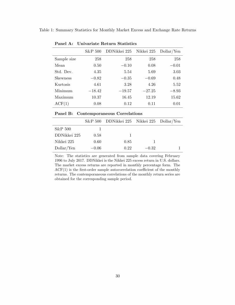
Table 1: Summary Statistics for Monthly Market Excess and Exchange Rate Returns

Panel A: Univariate Return Statistics

S&P 500 DDNikkei 225 Nikkei 225 Dollar/Yen

Sample size 258 258 258 258

Mean 0.50 −0.10 0.08 −0.01

Std. Dev. 4.35 5.54 5.69 3.03

Skewness −0.82 −0.35 −0.69 0.48

Kurtosis 4.61 3.28 4.26 5.52

Minimum −18.42 −19.57 −27.25 −8.93

Maximum 10.37 16.45 12.19 15.62

ACF(1) 0.08 0.12 0.11 0.01

Panel B: Contemporaneous Correlations

S&P 500 DDNikkei 225 Nikkei 225 Dollar/Yen

S&P 500 1

DDNikkei 225 0.58 1

Nikkei 225 0.60 0.85 1

Dollar/Yen −0.06 0.22 −0.32 1

Note: The statistics are generated from sample data covering February1996 to July 2017. DDNikkei is the Nikkei 225 excess return in U.S. dollars.The market excess returns are reported in monthly percentage form. TheACF(1) is the first-order sample autocorrelation coefficient of the monthlyreturns. The contemporaneous correlations of the monthly return series areobtained for the corresponding sample period.

30

Tab

le2:

Nik

kei

225

Ou

t-of

-th

e-M

oney

Ind

exO

pti

onD

ata

PanelA:

Sorted

by

Tim

e-to-m

atu

rity

τ[8,3

0)

[30,4

5)

[45,6

0)

[60,7

5)

[75,9

0)

All

Call

opti

on

Aver

age

num

ber

per

tradin

gday

10.6

014.2

215.7

515.7

814.7

336.4

2A

ver

age

per

centa

ge

bid

-ask

spre

ad

17.4

315.6

415.0

618.8

218.4

017.0

0A

ver

age

implied

vola

tility

24.8

523.0

222.6

221.8

321.4

122.8

2P

ut

opti

on

Aver

age

num

ber

per

tradin

gday

16.8

720.2

121.2

720.3

618.5

450.5

7A

ver

age

per

centa

ge

bid

-ask

spre

ad

17.2

313.8

612.9

515.4

615.2

615.0

0A

ver

age

implied

vola

tility

36.7

534.5

633.6

533.3

232.4

734.3

6

PanelB:

Sorted

by

OT

MP

ut

OT

MC

all

MoneynessK/F

<0.9

[0.9,0.9

7)

[0.9

7,1.0

3)

[1.0

3,1.1

)>

=1.1

All

Nea

r-te

rmopti

on

Aver

age

num

ber

per

tradin

gday

10.5

14.9

64.2

64.8

34.5

029.0

6A

ver

age

per

centa

ge

bid

-ask

spre

ad

23.1

77.1

14.0

011.6

028.5

316.5

3A

ver

age

implied

vola

tility

42.9

927.1

622.2

821.2

428.7

631.4

3N

ext-

term

opti

on

Aver

age

num

ber

per

tradin

gday

14.0

24.9

14.1

94.9

38.5

736.6

2A

ver

age

per

centa

ge

bid

-ask

spre

ad

18.2

24.9

83.5

66.0

924.6

714.6

4A

ver

age

implied

vola

tility

38.5

824.9

822.0

320.5

223.9

529.0

1

PanelC:

Sorted

by

OT

MP

ut,

τ∈

[8,4

4]

OT

MC

all,τ∈

[8,4

4]

log(K/F

)/(√τσATM

t)

<−

2.5

[−2.5,−

2.0

)[−

2.0,−

1.5

)[1.0,1.5

)>

=1.5

[Jan.

2006,

Nov

.2008

]A

ver

age

num

ber

per

wee

k14.1

94.8

84.8

86.8

612.8

1[

Dec

.2008,

Jun.

2017

]A

ver

age

num

ber

per

wee

k45.0

59.9

810.7

013.1

929.3

6

Note

:T

he

table

sum

mari

zes

the

Nik

kei

out-

of-

the-

money

index

opti

on

data

sort

edby

matu

rity

and

money

nes

sfr

om

January

2006

toJune

2017.

Panel

Are

port

sth

eav

erage

num

ber

of

OT

Mopti

ons

wit

hnon-z

ero

bid

and

ask

quote

sav

ailable

per

tradin

gday

,w

hen

ever

opti

ons

of

the

giv

ente

nor

cate

gory

are

traded

.T

he

aver

age

per

centa

ge

bid

-ask

spre

ad

isa

sim

ple

aver

age

of

100×

(ask−

bid

)/ask

.T

he

aver

age

implied

vola

tility

isth

eav

erage

of

the

annual

per

centa

ge

Bla

ck-S

chole

sim

plied

vola

tility

for

each

money

nes

sle

vel

(the

rati

oof

the

stri

ke

pri

ce,K

,to

forw

ard

pri

ce,F

).P

anel

Bre

port

sth

esa

me

thre

em

easu

res

for

the

nea

r-and

nex

t-te

rmopti

ons

sort

edby

money

nes

s.P

anel

Cpro

vid

esth

eav

erage

num

ber

of

short

er-d

ate

dopti

ons

available

per

wee

kas

afu

nct

ion

of

money

nes

s,w

her

eσATM

t

refe

rsto

the

end-o

f-day

tat-

the-

money

Bla

ckSch

ole

sim

plied

vola

tility

.

31

Table 3: Descriptive Statistics for the Variance Risk Premium and its Jump Tail Component

Panel A: Univariate statistics

V RP -US V RP -JPN LJV -US LJV -JPN

Sample size 210 138 258 138

Mean 0.14 0.39 0.05 0.05

Std. Dev. 0.16 0.55 0.05 0.06

Skewness 0.52 6.62 3.42 3.17

Kurtosis 12.27 57.76 17.71 15.70

Minimum −0.71 0.05 0.01 0.00

Maximum 0.99 5.50 0.37 0.43

ACF(1) 0.34 0.58 0.68 0.60

Panel B: Contemporaneous correlations

V RP -US V RP -JPN LJV -US LJV -JPN

V RP -US 1

V RP -JPN −0.17 1

LJV -US 0.03 0.76 1

LJV -JPN 0.17 0.22 0.49 1

Note: The monthly samples cover January 1996 to June 2017 forLJV -US, January 2000 to June 2017 for V RP -US and January2006 to June 2017 for the two Japanese series. They are reportedin monthly percentage form. The ACF(1) is the first-order sampleautocorrelation. The contemporaneous correlations are obtainedfor the period January 2006 to June 2017.

32

Tab

le4:

Cou

ntr

y-S

pec

ific

Sim

ple

Ret

urn

Pre

dic

tab

ilit

yR

egre

ssio

ns

Pan

el

A:

Pre

dic

ted

vari

ab

le:

S&

P500

excess

retu

rns

h1

23

45

67

89

10

11

12

Con

st0.4

20.2

30.2

60.2

20.

12

0.1

10.1

10.1

20.1

60.1

40.1

50.1

6

t(N

W)

(0.9

2)(0.5

3)(0.6

7)

(0.6

1)

(0.3

2)

(0.2

8)

(0.2

7)

(0.3

0)

(0.3

7)

(0.3

3)

(0.3

6)

(0.3

8)

LJV

-US

1.71

5.5

74.9

85.9

18.

09

8.2

78.4

88.1

67.3

97.7

77.4

87.3

3

t(N

W)

(0.1

8)(0.6

1)(0.6

3)

(0.9

4)

(1.9

3c)

(2.5

6b)

(2.7

2a)

(2.5

8b)

(2.0

8b)

(2.3

4b)

(2.3

2b)

(2.4

4b)

b(L

LS

W)

(0.2

2)(0.8

4)(0.8

4)

(1.1

9)

(2.3

4b)

(2.6

8b)

(2.6

9b)

(2.5

3b)

(2.0

3c)

(2.3

2b)

(2.3

3b)

(2.4

7b)

t(L

LS

W)

(0.2

2)(0.8

5)(0.8

7)

(1.2

7)

(2.6

0b)

(3.0

3a)

(3.0

0a)

(2.8

2b)

(2.2

1b)

(2.5

1b)

(2.5

1b)

(2.6

3b)

Ad

j.R

2−

0.36

0.2

60.4

01.0

32.

80

3.4

44.2

44.4

53.9

74.9

04.9

75.1

7

Pan

el

B:

Pre

dic

ted

vari

ab

le:

Nik

kei

225

excess

retu

rns

Con

st0.1

70.1

50.1

40.0

90.

09

0.0

50.0

70.1

30.1

60.1

20.1

20.1

0

t(N

W)

(0.2

3)(0.2

1)(0.1

9)

(0.1

2)

(0.1

2)

(0.0

7)

(0.0

9)

(0.1

7)

(0.2

1)

(0.1

7)

(0.1

6)

(0.1

4)

LJV

-JP

N1.

802.1

62.3

93.6

74.

15

5.2

15.1

24.0

53.5

14.1

84.3

34.5

8

t(N

W)

(0.2

8)(0.3

5)(0.3

5)

(0.5

3)

(0.5

7)

(0.7

7)

(0.8

3)

(0.6

8)

(0.6

2)

(0.7

7)

(0.8

3)

(0.9

0)

b(L

LS

W)

(0.2

3)(0.2

6)(0.2

9)

(0.4

6)

(0.5

3)

(0.7

3)

(0.8

1)

(0.6

8)

(0.6

4)

(0.8

1)

(0.8

9)

(0.9

8)

t(L

LS

W)

(0.2

4)(0.2

8)(0.3

0)

(0.4

7)

(0.5

4)

(0.7

5)

(0.8

3)

(0.7

0)

(0.6

5)

(0.8

2)

(0.8

9)

(0.9

7)

Ad

j.R

2−

0.70

−0.

64−

0.56

−0.

21

0.07

0.7

40.9

40.4

80.2

90.8

81.1

61.5

6

Not

e:T

he

tab

lere

por

tson

un

ivar

iate

pre

dic

tab

ilit

yre

gre

ssio

ns

for

aggre

gate

stock

exce

ssre

turn

sb

ase

don

ou

rlo

cal

jum

pta

ilri

skco

mp

onen

tof

theVRP

mea

sure

ineq

uati

on

(13).

Th

ep

red

icto

rsco

ver

Janu

ary

1996

toJu

ne

2017

for

U.S

.an

dJanu

ary

2006

toJu

ne

2017

for

Jap

an.

Inp

are

nth

eses

,w

ep

rese

ntt(

NW

),th

eN

Wt-

stati

stic

sw

ith

ala

gle

ngth

of

2h

,w

hil

eb(

LL

SW

)an

dt(

LL

SW

)ar

eth

eN

Wan

dE

WC

base

d-s

tati

stic

sp

rop

ose

dby

Laza

rus

etal.

(2018).

Th

esu

per

scri

ptsa,b

an

dc

ind

icate

the

sign

ifica

nce

level

s[p<

0.0

1],

[p<

0.05]

an

d[p<

0.1

],re

spec

tive

ly.

Th

ead

just

edR

2’s

are

rep

ort

edin

per

centa

ge

form

.

33

Table 5: Ratio of Foreign Investors on Trading Values

Year TSE 1st ETFs Nikkei 225 Nikkei 225 Nikkei 225Section stocks futures put options call options

2007 63.3 47.4 72.5 86.3 83.1

2008 64.8 47.8 78.7 86.1 85.6

2009 53.9 43.8 77.5 91.6 90.3

2010 63.6 54.5 76.7 89.7 88.9

2011 67.8 49.0 79.0 90.8 92.5

2012 67.7 51.4 77.4 93.7 92.9

2013 62.3 54.9 80.8 93.9 94.6

2014 69.1 53.9 81.0 92.9 94.3

2015 71.2 54.6 78.3 90.4 91.9

2016 73.8 62.9 79.5 92.5 93.9

2017 72.5 61.5 81.7 93.9 92.9

Note: This table reports the percentage of foreign investors in the total bro-kerage trading value (breakdown of brokerage). Survey by the Japan ExchangeGroup results from trading participants with capital of at least 3 billion yen, seehttps://www.jpx.co.jp/english/markets/statistics-equities/investor-type/00-02.htmland https://www.jpx.co.jp/english/markets/statistics-derivatives/sector/02.html fordetails.

34

Tab

le6:

Th

eD

olla

rD

enom

inat

edan

dL

oca

lN

ikke

i22

5R

etu

rnP

red

icta

bil

ity

Reg

ress

ion

s

Pan

el

A:

Pre

dic

ted

vari

able

:D

oll

ar

den

om

inate

dN

ikkei

225

excess

retu

rns,

Pre

dic

tor:

LJV

-US

h1

23

45

67

89

10

11

12

Con

st−

0.4

6−

0.7

3−

0.59

−0.

63

−0.

74

−0.

79

−0.8

2−

0.75

−0.

69

−0.6

7−

0.6

5−

0.6

3

t(N

W)

(−0.8

1)(−

1.3

4)(−

1.17)

(−1.

27)

(−1.

48)

(−1.

53)

(−1.

54)

(−1.

39)

(−1.

26)

(−1.2

3)

(−1.2

0)

(−1.1

5)

LJV

-US

7.35

12.9

210.0

810.

94

13.

34

14.

47

15.

23

14.

00

12.

72

12.

49

12.

28

11.

87

t(N

W)

(0.8

0)(1.6

5c)

(1.4

9)

(1.8

5c)

(3.0

0a)

(3.7

0a)

(3.9

4a)

(3.7

0a)

(3.2

8a)

(3.2

7a)

(3.1

5a)

(2.9

8a)

b(L

LS

W)

(1.1

7)(2.1

1c)

(1.8

0c)

(2.1

2c)

(3.1

1a)

(3.5

6a)

(3.7

2a)

(3.5

3a)

(3.1

9a)

(3.2

3a)

(3.1

9a)

(3.0

9a)

t(L

LS

W)

(1.2

8)(2.5

0b)

(2.1

4b)

(2.4

7b)

(3.6

0a)

(3.9

1a)

(3.9

7a)

(3.7

5a)

(3.3

7a)

(3.4

2a)

(3.4

1a)

(3.2

9a)

Ad

j.R

2−

0.0

11.

701.

50

2.36

4.57

6.34

8.08

7.67

6.90

7.18

7.52

7.63

Pan

el

B:

Pre

dic

ted

vari

ab

le:

Yen

den

om

inate

dN

ikkei

225

excess

retu

rns,

Pre

dic

tor:

LJV

-US

Con

st0.0

2−

0.2

3−

0.18

−0.

30

−0.

39

−0.

43

−0.

43

−0.

35

−0.

28

−0.2

5−

0.2

2−

0.2

2

t(N

W)

(0.0

3)(−

0.44

)(−

0.35)

(−0.

59)

(−0.

71)

(−0.

75)

(−0.

75)

(−0.

60)

(−0.4

8)

(−0.4

2)

(−0.3

8)

(−0.3

8)

LJV

-US

1.29

6.47

5.29

7.92

9.76

10.

62

10.

87

9.38

7.92

7.33

6.80

6.82

t(N

W)

(0.1

7)(1.0

3)(0.9

8)

(1.7

4c)

(2.4

0b)

(2.6

3a)

(2.6

7a)

(2.2

1b)

(1.7

7c)

(1.7

0c)

(1.6

7c)

(1.7

4c)

b(L

LS

W)

(0.2

1)(1.3

6)(1.1

7)

(1.8

7c)

(2.2

8b)

(2.3

8b)

(2.4

4b)

(2.0

7c)

(1.7

1)

(1.6

8)

(1.6

8)

(1.7

9c)

t(L

LS

W)

(0.2

3)(1.6

3)(1.4

2)

(2.2

3b)

(2.4

7b)

(2.5

3b)

(2.5

8b)

(2.1

7b)

(1.7

9c)

(1.7

6c)

(1.7

6c)

(1.8

7c)

Ad

j.R

2−

0.3

80.

110.

08

0.95

2.06

3.00

3.73

3.13

2.41

2.24

2.07

2.28

Pan

el

C:

Pre

dic

ted

vari

ab

le:

Doll

ar

den

om

inate

dN

ikkei

225

excess

retu

rns,

Pre

dic

tor:

LJV

-JP

N

Con

st0.0

60.

080.

03

−0.

05

−0.

04

−0.

05

−0.

01

0.06

0.11

0.10

0.12

0.12

t(N

W)

(0.1

1)(0.1

6)(0.0

7)

(−0.

10)

(−0.

08)

(−0.

09)

(−0.

02)

(0.1

2)

(0.2

2)

(0.2

1)

(0.2

4)

(0.2

4)

LJV

-JP

N3.

413.

033.

84

5.62

5.89

6.33

6.02

4.83

4.02

4.29

4.09

4.14

t(N

W)

(0.5

6)(0.5

5)(0.6

6)

(0.9

5)

(0.9

2)

(0.9

8)

(0.9

7)

(0.8

2)

(0.7

3)

(0.8

5)

(0.8

5)

(0.8

9)

b(L

LS

W)

(0.5

8)(0.4

8)(0.5

9)

(0.8

5)

(0.8

5)

(0.9

3)

(0.9

5)

(0.8

2)

(0.7

5)

(0.8

9)

(0.9

1)

(0.9

7)

t(L

LS

W)

(0.6

2)(0.5

0)(0.6

0)

(0.8

6)

(0.8

6)

(0.9

4)

(0.9

6)

(0.8

3)

(0.7

6)

(0.9

1)

(0.9

3)

(0.9

9)

Ad

j.R

2−

0.5

1−

0.4

20.

07

1.59

2.38

3.49

3.78

2.64

1.91

2.61

2.66

3.19

Not

e:T

he

tab

lere

por

tson

un

ivar

iate

pre

dic

tab

ilit

yre

gre

ssio

ns

for

aggre

gate

stock

exce

ssre

turn

sb

ase

don

ou

rlo

cal

jum

pta

ilri

skco

mp

onen

tof

theVRP

mea

sure

ineq

uati

on

(13)

for

the

U.S

.or

Jap

an

.T

he

pre

dic

tors

cove

rJanu

ary

1996

toJu

ne

2017

for

U.S

.an

dJan

uar

y20

06to

Ju

ne

2017

for

Jap

an

.In

pare

nth

eses

,w

ep

rese

ntt(

NW

),th

eN

Wt-

stati

stic

sw

ith

ala

gle

ngth

of

2h,

wh

ile

b(L

LS

W)

andt(

LL

SW

)ar

eth

eN

Wan

dE

WC

base

d-s

tati

stic

sp

rop

ose

dby

Laza

rus

etal.

(2018).

Th

esu

per

scri

ptsa,b

an

dc

ind

icate

the

sign

ifica

nce

leve

ls[p<

0.01

],[p<

0.05]

an

d[p<

0.1],

resp

ecti

vely

.T

he

ad

just

edR

2’s

are

rep

ort

edin

per

centa

ge

form

.

35

Figure 1: Slopes of the OTM Nikkei 225 Index Put Decay

­0.5 ­0.4 ­0.3 ­0.2 ­0.1 0.0

10

20

30

­0.5 ­0.4 ­0.3 ­0.2 ­0.1 0.0

10

20

30

­0.5 ­0.4 ­0.3 ­0.2 ­0.1 0.0

10

20

30

­0.5 ­0.4 ­0.3 ­0.2 ­0.1 0.0

10

20

30

Panel A

Panel C

Panel B

Panel D

Panel E

­0.5 ­0.4 ­0.3 ­0.2 ­0.1 0.0

10

20

30

­0.5 ­0.4 ­0.3 ­0.2 ­0.1 0.0

10

20

30

Panel F

Panel G Panel H

­0.5 ­0.4 ­0.3 ­0.2 ­0.1 0.0

10

20

30

­0.5 ­0.4 ­0.3 ­0.2 ­0.1 0.0

10

20

30

Note: The figure plots estimated weekly slopes of the OTM put decay, obtained as

log(Ot,τ (kt,i)/Ot,τ (kt,i−1))/(kt,i − kt,i−1) against log-moneyness kt,i under the assumption that the

shape of the left jump tails are constant over each individual week. The flat dotted lines represent the

estimated values of 1 + α−. The plots are obtained by pooling the selected Nikkei 225 OTM put options

over the week from January 18 to 24, 2006 (Panel A), December 8 to 14, 2007 (Panel B), November 22 to

28, 2008 (Panel C), December 10 to 16, 2008 (Panel D), March 25 to 31, 2011 (Panel E), August 16 to 22,

2014 (Panel F), September 3 to 9, 2015 (Panel G), and June 10 to 16, 2017 (Panel H), respectively.

36

Figure 2: Plots of Left Jump Tail Estimates of 1/α−t

1996 1998 2000 2002 2004 2006 2008 2010 2012 2014 2016 2018

0.1

0.2

Lehman Shock

US Flash Crash

Tohoku Earthquake and Tsunami

World wide stock price drop

Increasing uncertainty regarding Abenomics

October 27, 1997, minicrash and Asian financial crisis

Russian crisis and LTCM shock

Dotcom bubble burst

The 9/11 Attacks and 2001 Recession

Chinese and global market turbulence

Note: The figure plots the estimates of 1/α−t at a monthly frequency over the sample from January 1996 to

June 2017 for U.S. (solid line) and January 2006 to June 2017 for Japan (dashed line).

37

Figure 3: Plots of Variance Risk Premium and its Jump Tail Component

VRP­US VRP­JPN

1996 1998 2000 2002 2004 2006 2008 2010 2012 2014 2016 2018

0

25

50

VRP­US VRP­JPN

LJV­US LJV­JPN

1996 1998 2000 2002 2004 2006 2008 2010 2012 2014 2016 2018

1

2

3

4

5Lehman Shock

US Flash Crash

Tohoku Earthquake and Tsunami

World wide stock price drop

Increasing uncertainty regarding Abenomics

October 27, 1997, minicrash andAsian financial crisis

Russian crisis and LTCM shock

Dotcom bubble burst

The 9/11 Attacks and 2001 Recession Chinese and global

market turbulence

LJV­US LJV­JPN

Note: The series are plotted at a monthly frequency. They span January 1996 to June 2017 for LJV -US,

January 2000 to June 2017 for V RP -US, and January 2006 to June 2017 for Japan. They are reported in

annualized percentage form.

38

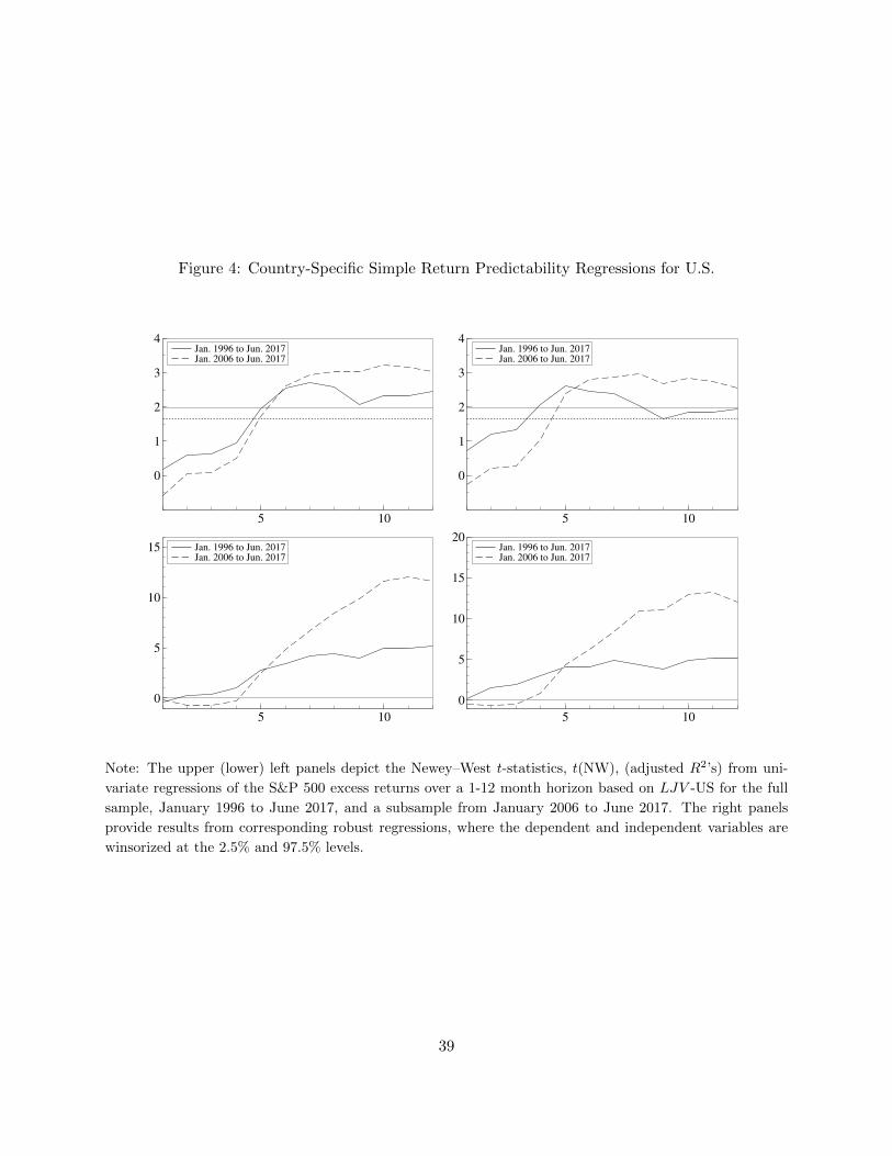
Figure 4: Country-Specific Simple Return Predictability Regressions for U.S.

Jan. 1996 to Jun. 2017

Jan. 2006 to Jun. 2017

5 10

0

1

2

3

4Jan. 1996 to Jun. 2017

Jan. 2006 to Jun. 2017

Jan. 1996 to Jun. 2017

Jan. 2006 to Jun. 2017

5 10

0

1

2

3

4Jan. 1996 to Jun. 2017

Jan. 2006 to Jun. 2017

Jan. 1996 to Jun. 2017

Jan. 2006 to Jun. 2017

5 10

0

5

10

15 Jan. 1996 to Jun. 2017

Jan. 2006 to Jun. 2017

Jan. 1996 to Jun. 2017

Jan. 2006 to Jun. 2017

5 10

0

5

10

15

20Jan. 1996 to Jun. 2017

Jan. 2006 to Jun. 2017

Note: The upper (lower) left panels depict the Newey–West t-statistics, t(NW), (adjusted R2’s) from uni-

variate regressions of the S&P 500 excess returns over a 1-12 month horizon based on LJV -US for the full

sample, January 1996 to June 2017, and a subsample from January 2006 to June 2017. The right panels

provide results from corresponding robust regressions, where the dependent and independent variables are

winsorized at the 2.5% and 97.5% levels.

39

Figure 5: Country-Specific Simple Return Predictability Regressions for Japan.

No winsorization

Winsorization

5 10

0

2

No winsorization

Winsorization

No winsorization

Winsorization

5 10

0

10

20

No winsorization

Winsorization

Note: The left and right panels depict the Newey–West t-statistics, t(NW), and adjusted R2’s from univariate

regressions of the Nikkei 225 excess returns over a 1-12 month horizon based on LJV -JPN from January

2006 to June 2017. The solid lines are based on the regression results in Panel B of Table 4. The dashed

lines represent results from corresponding robust regressions using the dependent and independent variables

winsorized at the 2.5% and 97.5% levels.

40

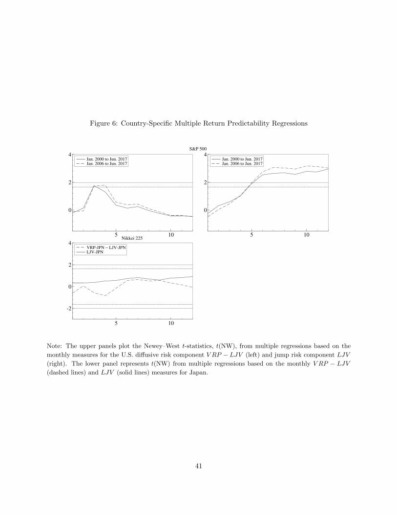
Figure 6: Country-Specific Multiple Return Predictability Regressions

Jan. 2000 to Jun. 2017

Jan. 2006 to Jun. 2017

5 10

0

2

4

S&P 500

Jan. 2000 to Jun. 2017

Jan. 2006 to Jun. 2017

Jan. 2000 to Jun. 2017

Jan. 2006 to Jun. 2017

5 10

0

2

4Jan. 2000 to Jun. 2017

Jan. 2006 to Jun. 2017

VRP­JPN − LJV­JPN

LJV­JPN

5 10

­2

0

2

4

Nikkei 225

VRP­JPN − LJV­JPN

LJV­JPN

Note: The upper panels plot the Newey–West t-statistics, t(NW), from multiple regressions based on the

monthly measures for the U.S. diffusive risk component V RP − LJV (left) and jump risk component LJV

(right). The lower panel represents t(NW) from multiple regressions based on the monthly V RP − LJV(dashed lines) and LJV (solid lines) measures for Japan.

41

Figure 7: Dollar- and Yen-Denominated Nikkei 225 Return Regressions Based on LJV -US

Jan. 1996 to Jun. 2017

Jan. 2006 to Jun. 2017

5 10

0

1

2

3

4DDNikkei

Jan. 1996 to Jun. 2017

Jan. 2006 to Jun. 2017

Jan. 1996 to Jun. 2017

Jan. 2006 to Jun. 2017

5 10

0

1

2

3

4Nikkei

Jan. 1996 to Jun. 2017

Jan. 2006 to Jun. 2017

Jan. 1996 to Jun. 2017

Jan. 2006 to Jun. 2017

5 10

0

5

10

15

20Jan. 1996 to Jun. 2017

Jan. 2006 to Jun. 2017

Jan. 1996 to Jun. 2017

Jan. 2006 to Jun. 2017

5 10

0

5

10

15

20Jan. 1996 to Jun. 2017

Jan. 2006 to Jun. 2017

Note: The upper (lower) left and right panels depict the Newey–West t-statistics, t(NW) (adjusted R2’s),

from univariate regressions of the dollar-denominated and local (yen-denominated) Nikkei 225 excess returns

over a 1-12 month horizon based on LJV -US for the full sample, January 1996 to June 2017, and a subsample,

January 2006 to June 2017, respectively.

42

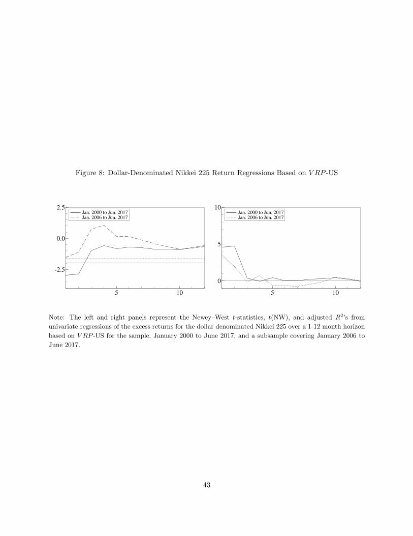
Figure 8: Dollar-Denominated Nikkei 225 Return Regressions Based on V RP -US

Jan. 2000 to Jun. 2017

Jan. 2006 to Jun. 2017

5 10

­2.5

0.0

2.5Jan. 2000 to Jun. 2017

Jan. 2006 to Jun. 2017

Jan. 2000 to Jun. 2017

Jan. 2006 to Jun. 2017

5 10

0

5

10Jan. 2000 to Jun. 2017

Jan. 2006 to Jun. 2017

Note: The left and right panels represent the Newey–West t-statistics, t(NW), and adjusted R2’s from

univariate regressions of the excess returns for the dollar denominated Nikkei 225 over a 1-12 month horizon

based on V RP -US for the sample, January 2000 to June 2017, and a subsample covering January 2006 to

June 2017.

43

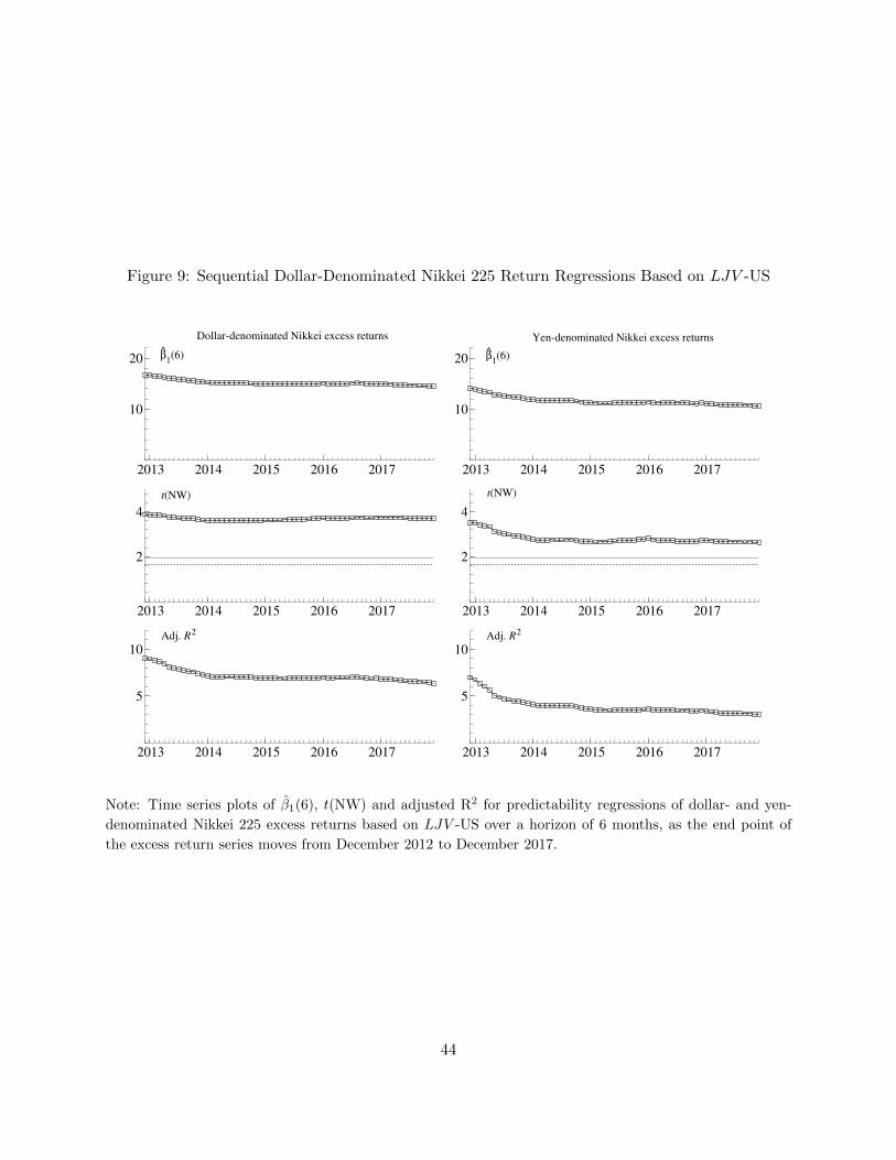
Figure 9: Sequential Dollar-Denominated Nikkei 225 Return Regressions Based on LJV -US

2013 2014 2015 2016 2017

10

20 β1(6)

Dollar­denominated Nikkei excess returns

2013 2014 2015 2016 2017

10

20 β1(6)

Yen­denominated Nikkei excess returns

2013 2014 2015 2016 2017

2

4

t(NW)

2013 2014 2015 2016 2017

2

4

t(NW)

2013 2014 2015 2016 2017

5

10Adj. R2

2013 2014 2015 2016 2017

5

10Adj. R2

Note: Time series plots of β1(6), t(NW) and adjusted R2 for predictability regressions of dollar- and yen-

denominated Nikkei 225 excess returns based on LJV -US over a horizon of 6 months, as the end point of

the excess return series moves from December 2012 to December 2017.

44

Figure 10: Dollar-Yen Exchange Rate Return Predictability Based on LJV -US

No winsorization

Winsorization

5 10

0

2

No winsorization

Winsorization

No winsorization

Winsorization

5 10

0

5

10No winsorization

Winsorization

Note: The left and right panels plot the Newey–West t-statistics, t(NW), and adjusted R2’s from univariate

regressions of the dollar-yen exchange rate returns over a 1-12 month horizon based on LJV -US for the full

sample, January 1996 to June 2017 (solid lines). The dashed lines represent results from robust regressions

using the dependent and independent variables winsorized at the 2.5% and 97.5% levels.

Figure 11: Dollar-Yen Exchange Rate Return Predictability Based on Diffusive and Jump RiskComponents of V RP -US

VRP­US − LJV­US

LJV­US

5 10

0

2

VRP­US − LJV­US

LJV­US

5 10

0

5

10

Note: The left panels represent the Newey–West t-statistics, t(NW), from multiple return predictability

regressions of the dollar-yen exchange rates over a 1-12 month horizon based on the diffusive risk component,

V RP -US − LJV -US, and jump risk component LJV -US for the sample from January 2000 to June 2017.

The right panels plot the corresponding adjusted R2’s.

45