System Design and Assessment Notes Note 43 RF DEW Scenarios and Threat...

System Design and Assessment Notes

Note 43

RF DEW Scenarios and Threat Analysis

Dr. Frank Peterkin Dr. Robert L. Gardner, Consultant

Directed Energy Warfare Office Naval Surface Warfare Center

Dahlgren, VA 22222 USA

ABSTRACT High power microwave weapons interact with their targets in complex ways. That interaction can best be described as a sequence of transfer functions describing the HPM source, antenna, propagation to the target, external target response, penetration into the target and finally the response of the target circuitry. This paper first describes these various transfer functions in a qualitative way. Prediction of the actual target is response is usually done empirically and some of the publicly available data is described and used to support the description of various scenarios. The paper concludes with three scenarios across seven sources and broad estimates are given for the effectiveness of the candidate sources.

RF DEW SCENARIOS AND THREAT ANALYSIS

1. INTRODUCTION

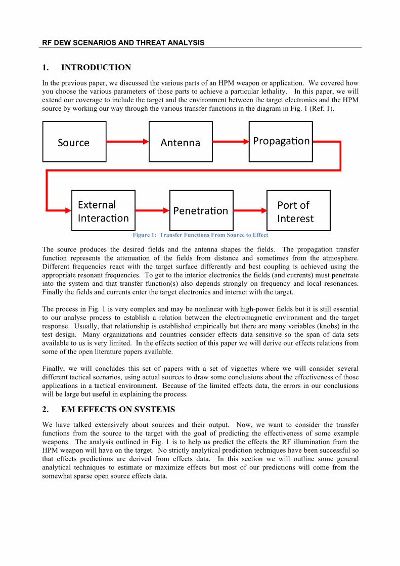
In the previous paper, we discussed the various parts of an HPM weapon or application. We covered how you choose the various parameters of those parts to achieve a particular lethality. In this paper, we will extend our coverage to include the target and the environment between the target electronics and the HPM source by working our way through the various transfer functions in the diagram in Fig. 1 (Ref. 1).

Figure 1: Transfer Functions From Source to Effect

The source produces the desired fields and the antenna shapes the fields. The propagation transfer function represents the attenuation of the fields from distance and sometimes from the atmosphere. Different frequencies react with the target surface differently and best coupling is achieved using the appropriate resonant frequencies. To get to the interior electronics the fields (and currents) must penetrate into the system and that transfer function(s) also depends strongly on frequency and local resonances. Finally the fields and currents enter the target electronics and interact with the target. The process in Fig. 1 is very complex and may be nonlinear with high-power fields but it is still essential to our analyse process to establish a relation between the electromagnetic environment and the target response. Usually, that relationship is established empirically but there are many variables (knobs) in the test design. Many organizations and countries consider effects data sensitive so the span of data sets available to us is very limited. In the effects section of this paper we will derive our effects relations from some of the open literature papers available. Finally, we will concludes this set of papers with a set of vignettes where we will consider several different tactical scenarios, using actual sources to draw some conclusions about the effectiveness of those applications in a tactical environment. Because of the limited effects data, the errors in our conclusions will be large but useful in explaining the process.

2. EM EFFECTS ON SYSTEMS

We have talked extensively about sources and their output. Now, we want to consider the transfer functions from the source to the target with the goal of predicting the effectiveness of some example weapons. The analysis outlined in Fig. 1 is to help us predict the effects the RF illumination from the HPM weapon will have on the target. No strictly analytical prediction techniques have been successful so that effects predictions are derived from effects data. In this section we will outline some general analytical techniques to estimate or maximize effects but most of our predictions will come from the somewhat sparse open source effects data.


2.1 Source The source, as shown in the previous paper, transmits the radio frequency fields. For this section of the paper, the source fields will be derived from chosen HPM weapon applications and combined with the antenna on the application to predict the field at the assumed target.

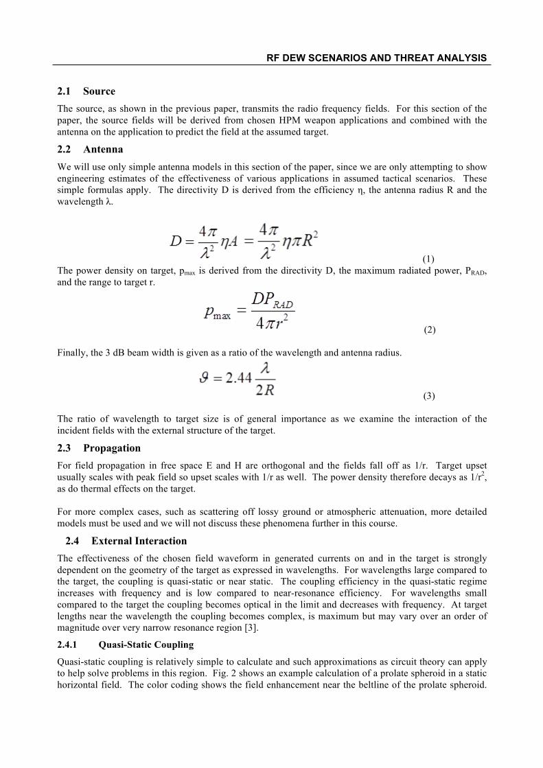
2.2 Antenna We will use only simple antenna models in this section of the paper, since we are only attempting to show engineering estimates of the effectiveness of various applications in assumed tactical scenarios. These simple formulas apply. The directivity D is derived from the efficiency η, the antenna radius R and the wavelength λ.

(1) The power density on target, pmax is derived from the directivity D, the maximum radiated power, PRAD, and the range to target r.

(2) Finally, the 3 dB beam width is given as a ratio of the wavelength and antenna radius.

(3) The ratio of wavelength to target size is of general importance as we examine the interaction of the incident fields with the external structure of the target.

2.3 Propagation For field propagation in free space E and H are orthogonal and the fields fall off as 1/r. Target upset usually scales with peak field so upset scales with 1/r as well. The power density therefore decays as 1/r2, as do thermal effects on the target. For more complex cases, such as scattering off lossy ground or atmospheric attenuation, more detailed models must be used and we will not discuss these phenomena further in this course.

2.4 External Interaction The effectiveness of the chosen field waveform in generated currents on and in the target is strongly dependent on the geometry of the target as expressed in wavelengths. For wavelengths large compared to the target, the coupling is quasi-static or near static. The coupling efficiency in the quasi-static regime increases with frequency and is low compared to near-resonance efficiency. For wavelengths small compared to the target the coupling becomes optical in the limit and decreases with frequency. At target lengths near the wavelength the coupling becomes complex, is maximum but may vary over an order of magnitude over very narrow resonance region [3].

2.4.1 Quasi-Static Coupling

Quasi-static coupling is relatively simple to calculate and such approximations as circuit theory can apply to help solve problems in this region. Fig. 2 shows an example calculation of a prolate spheroid in a static horizontal field. The color coding shows the field enhancement near the beltline of the prolate spheroid.


We can use this type of estimate to show the field enhancement on a desktop computer in an EMP (wavelengths much larger than a computer but near resonance for power cables) field.

Figure 2: Prolate spheroid illuminated by horizontal field. Fields enhanced on beltline.

2.4.2 Resonant Coupling

Resonant coupling is the most complicated but most efficient. Fig. 3 shows a very simple calculation from NEC4. The target is a simple dipole illuminated by a dipole field. For the resonant case, the induced currents are much larger than for the case where the excitation is about 10% off resonance.

Figure 3: Dipole response to resonant and near resonant fields

2.4.3 Optical or Diffractive Coupling

When the incident wavelength is small compared to the target, coupling calculations become much less complicated and such concepts as shadowing and diffraction become useful for estimates. Fig. 4 shows a source sending a wave toward a cylinder. Waves diffract around the cylinder and the fields at the observation point are much smaller than the incident fields but still non zero.


Figure 4: Optical and Diffractive Coupling

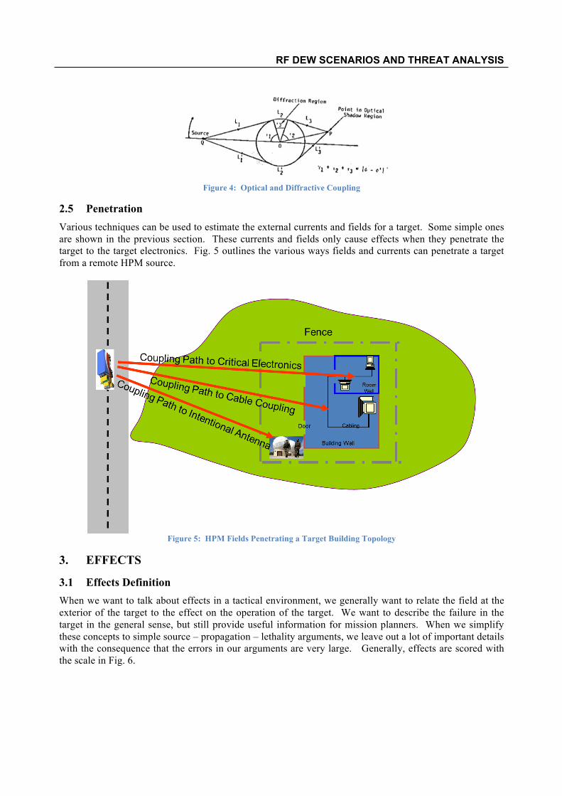
2.5 Penetration Various techniques can be used to estimate the external currents and fields for a target. Some simple ones are shown in the previous section. These currents and fields only cause effects when they penetrate the target to the target electronics. Fig. 5 outlines the various ways fields and currents can penetrate a target from a remote HPM source.

Figure 5: HPM Fields Penetrating a Target Building Topology

3. EFFECTS

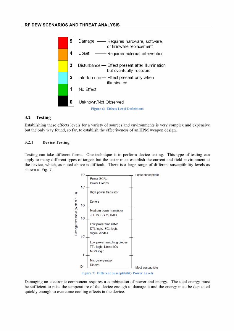
3.1 Effects Definition When we want to talk about effects in a tactical environment, we generally want to relate the field at the exterior of the target to the effect on the operation of the target. We want to describe the failure in the target in the general sense, but still provide useful information for mission planners. When we simplify these concepts to simple source – propagation – lethality arguments, we leave out a lot of important details with the consequence that the errors in our arguments are very large. Generally, effects are scored with the scale in Fig. 6.


Figure 6: Effects Level Definitions

3.2 Testing Establishing these effects levels for a variety of sources and environments is very complex and expensive but the only way found, so far, to establish the effectiveness of an HPM weapon design.

3.2.1 Device Testing

Testing can take different forms. One technique is to perform device testing. This type of testing can apply to many different types of targets but the tester must establish the current and field environment at the device, which, as noted above is difficult. There is a large range of different susceptibility levels as shown in Fig. 7.

Figure 7: Different Susceptibility Power Levels

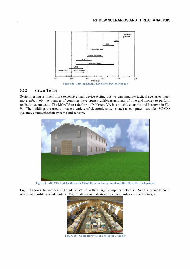
Damaging an electronic component requires a combination of power and energy. The total energy must be sufficient to raise the temperature of the device enough to damage it and the energy must be deposited quickly enough to overcome cooling effects in the device.


Figure 8: Varying Energy Levels for Device Damage

3.2.2 System Testing

System testing is much more expensive than device testing but we can simulate tactical scenarios much more effectively. A number of countries have spent significant amounts of time and money to perform realistic system tests. The MOATS test facility at Dahlgren, VA is a notable example and is shown in Fig. 9. The buildings are used to house a variety of electronic systems such as computer networks, SCADA systems, communication systems and sensors.

Figure 9: MOATS Test Facility with Citadelle in the Foreground and Bastille in the Background

Fig. 10 shows the interior of Citadelle set up with a large computer network. Such a network could represent a military headquarters. Fig. 11 shows an industrial process simulator – another target.

Figure 10: Computer Network Setup in Citadelle


Figure 11: Industrial Process Trainer

3.3 Effects Testing in the Literature Results for much of the testing shown here is considered sensitive by the testers, but some testers, primarily in Europe, have published their results. Some examples are shown in Table 1. Table 1: Some Published Effects Test Results


These test reports provide a span of results and show that those concerned with protecting their equipment need to start worrying at levels as low as a few 10s of V/m.

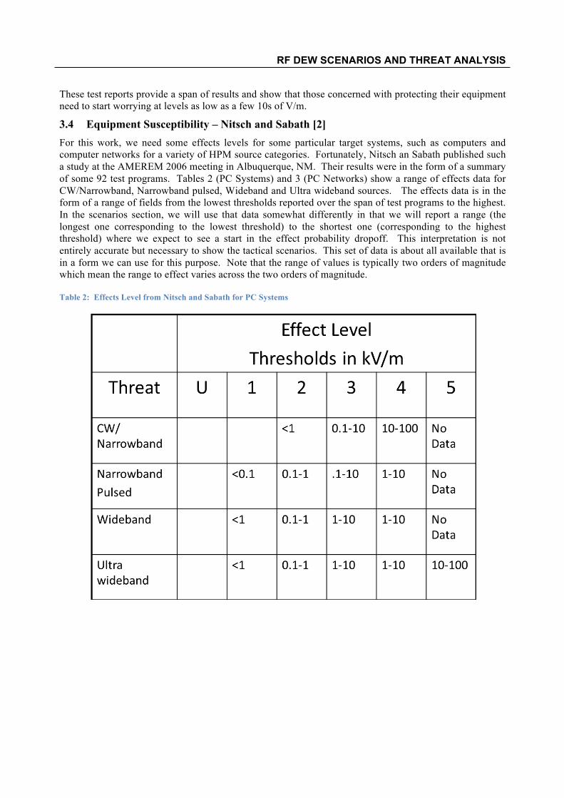
3.4 Equipment Susceptibility – Nitsch and Sabath [2] For this work, we need some effects levels for some particular target systems, such as computers and computer networks for a variety of HPM source categories. Fortunately, Nitsch an Sabath published such a study at the AMEREM 2006 meeting in Albuquerque, NM. Their results were in the form of a summary of some 92 test programs. Tables 2 (PC Systems) and 3 (PC Networks) show a range of effects data for CW/Narrowband, Narrowband pulsed, Wideband and Ultra wideband sources. The effects data is in the form of a range of fields from the lowest thresholds reported over the span of test programs to the highest. In the scenarios section, we will use that data somewhat differently in that we will report a range (the longest one corresponding to the lowest threshold) to the shortest one (corresponding to the highest threshold) where we expect to see a start in the effect probability dropoff. This interpretation is not entirely accurate but necessary to show the tactical scenarios. This set of data is about all available that is in a form we can use for this purpose. Note that the range of values is typically two orders of magnitude which mean the range to effect varies across the two orders of magnitude. Table 2: Effects Level from Nitsch and Sabath for PC Systems


Table 3: Effects Data from Nitsch and Sabath for PC Networks

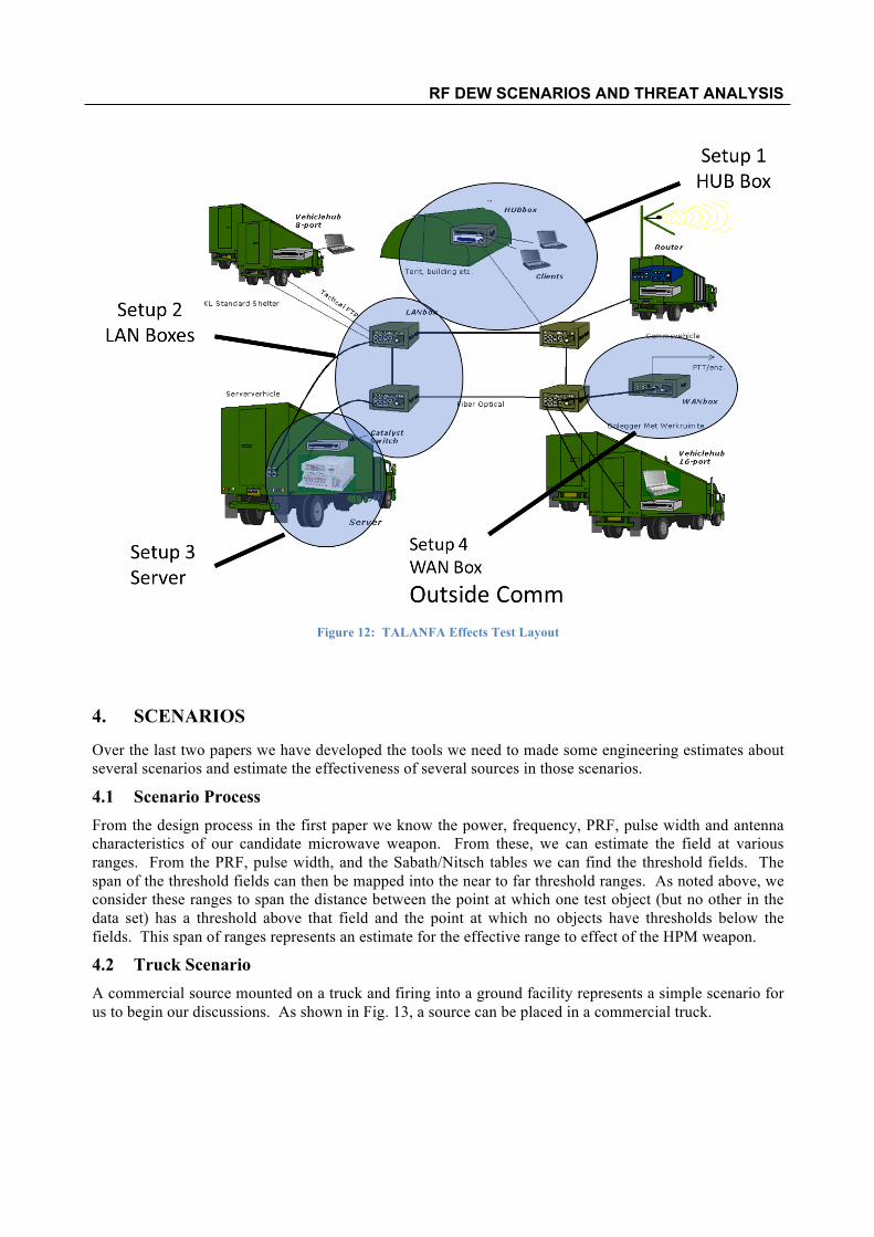
3.5 Susceptibility - TALANFA Our NATO group also performed a series of system tests on a fielded military computer network called TALANFA [1]. The testing was done in 5 countries and 6 test facilities. The various test configurations are outlined in Fig. 12. Unlike EMP, HPM source illumination does not cover the entire system so four different illumination configurations were designed and used for testing. Every effort was made to make that data from one test facility could be compared with the data from the others. Unfortunately, the data from this data set cannot be shared in this forum, we learned a lot about setting up tests that can be used to develop comparison techniques.


Figure 12: TALANFA Effects Test Layout

4. SCENARIOS

Over the last two papers we have developed the tools we need to made some engineering estimates about several scenarios and estimate the effectiveness of several sources in those scenarios.

4.1 Scenario Process From the design process in the first paper we know the power, frequency, PRF, pulse width and antenna characteristics of our candidate microwave weapon. From these, we can estimate the field at various ranges. From the PRF, pulse width, and the Sabath/Nitsch tables we can find the threshold fields. The span of the threshold fields can then be mapped into the near to far threshold ranges. As noted above, we consider these ranges to span the distance between the point at which one test object (but no other in the data set) has a threshold above that field and the point at which no objects have thresholds below the fields. This span of ranges represents an estimate for the effective range to effect of the HPM weapon.

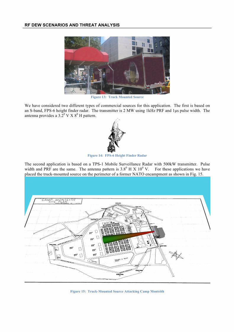
4.2 Truck Scenario A commercial source mounted on a truck and firing into a ground facility represents a simple scenario for us to begin our discussions. As shown in Fig. 13, a source can be placed in a commercial truck.


Figure 13: Truck Mounted Source

We have considered two different types of commercial sources for this application. The first is based on an S-band, FPS-6 height finder radar. The transmitter is 2 MW using 1kHz PRF and 1µs pulse width. The antenna provides a 3.20 V X 80 H pattern.

Figure 14: FPS-6 Height Finder Radar

The second application is based on a TPS-1 Mobile Surveillance Radar with 500kW transmitter. Pulse width and PRF are the same. The antenna pattern is 3.80 H X 100 V. For these applications we have placed the truck-mounted source on the perimeter of a former NATO encampment as shown in Fig. 15.

Figure 15: Truck-Mounted Source Attacking Camp Monteith


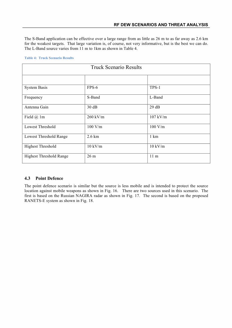
The S-Band application can be effective over a large range from as little as 26 m to as far away as 2.6 km for the weakest targets. That large variation is, of course, not very informative, but is the best we can do. The L-Band source varies from 11 m to 1km as shown in Table 4. Table 4: Truck Scenario Results

Truck Scenario Results

System Basis FPS-6 TPS-1

Frequency S-Band L-Band

Antenna Gain 30 dB 29 dB

Field @ 1m 260 kV/m 107 kV/m

Lowest Threshold 100 V/m 100 V/m

Lowest Threshold Range 2.6 km 1 km

Highest Threshold 10 kV/m 10 kV/m

Highest Threshold Range 26 m 11 m

4.3 Point Defence The point defence scenario is similar but the source is less mobile and is intended to protect the source location against mobile weapons as shown in Fig. 16. There are two sources used in this scenario. The first is based on the Russian NAGIRA radar as shown in Fig. 17. The second is based on the proposed RANETS-E system as shown in Fig. 18.


Figure 16: Point Defence Scenario

Figure 17: NAGIRA Radar


Figure 18: RANETS- E Brochure

The result of the point defence scenario is similar in style to that of the truck-mounted source scenario but with somewhat longer ranges. The short pulse width of these sources limits their effectiveness but the large antenna gains and high power more than compensate. Table 5: Point Defence Scenario Results

Point Defence Scenario Results

System Basis NAGIRA RANETS-E

Frequency X-Band X-Band

Antenna Gain 32 dB 52 dB

Field @ 1m 4600 kV/m 48000 kV/m

Lowest Threshold 100 V/m 100 V/m


Lowest Threshold Range 46 km 486 km

Highest Threshold 10 kV/m 10 kV/m

Highest Threshold Range 460 m 4.8 km

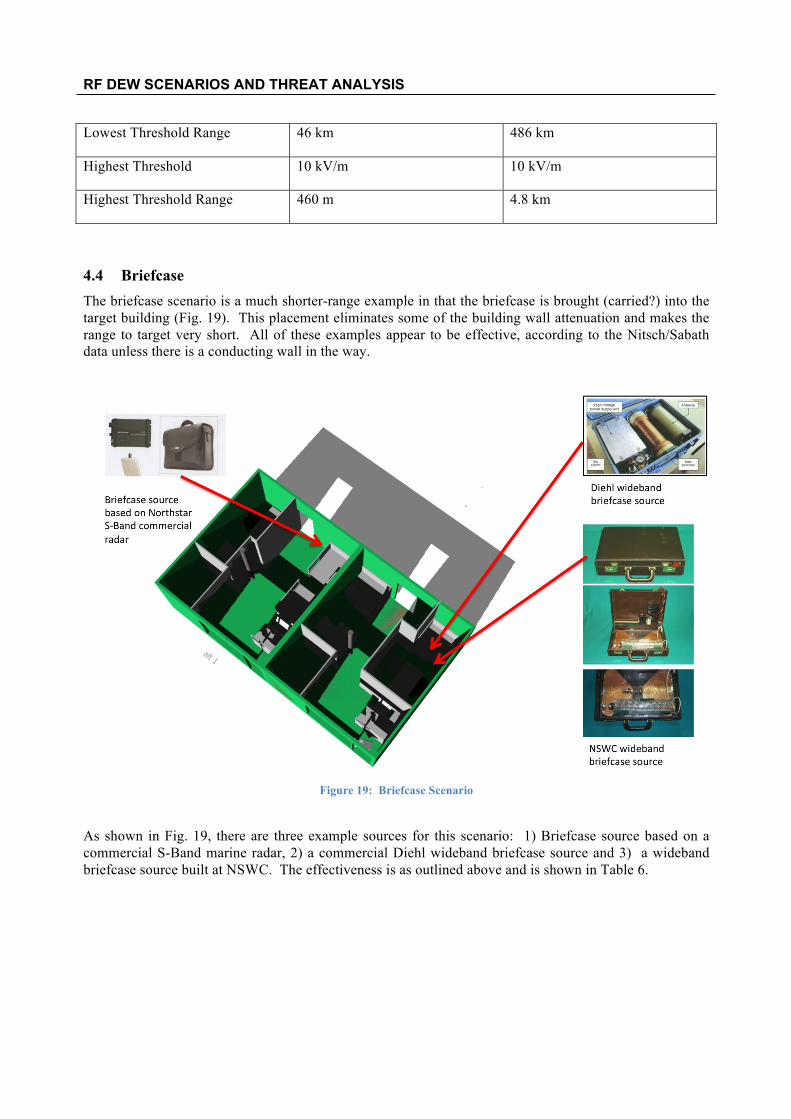
4.4 Briefcase The briefcase scenario is a much shorter-range example in that the briefcase is brought (carried?) into the target building (Fig. 19). This placement eliminates some of the building wall attenuation and makes the range to target very short. All of these examples appear to be effective, according to the Nitsch/Sabath data unless there is a conducting wall in the way.

Figure 19: Briefcase Scenario

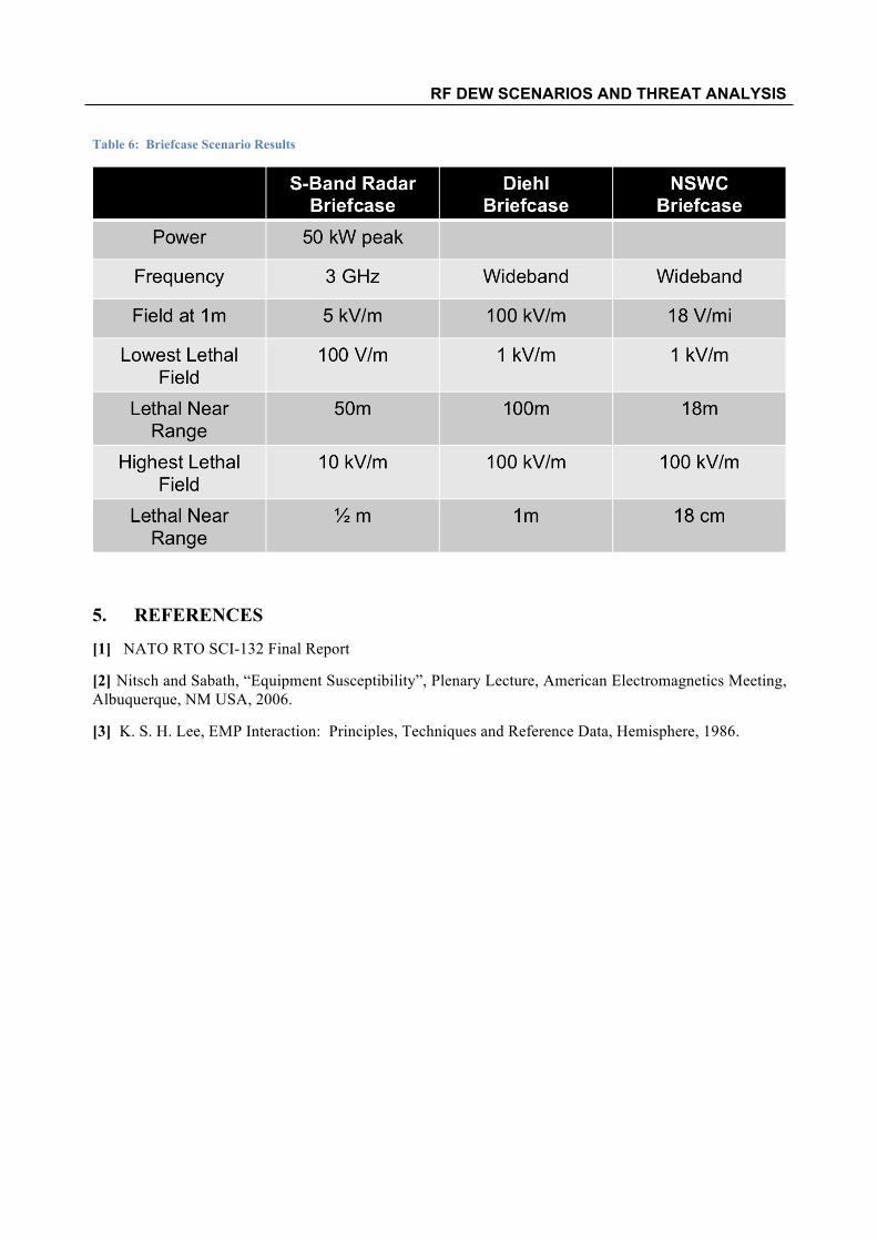
As shown in Fig. 19, there are three example sources for this scenario: 1) Briefcase source based on a commercial S-Band marine radar, 2) a commercial Diehl wideband briefcase source and 3) a wideband briefcase source built at NSWC. The effectiveness is as outlined above and is shown in Table 6.


Table 6: Briefcase Scenario Results

5. REFERENCES

[1] NATO RTO SCI-132 Final Report

[2] Nitsch and Sabath, “Equipment Susceptibility”, Plenary Lecture, American Electromagnetics Meeting, Albuquerque, NM USA, 2006.

[3] K. S. H. Lee, EMP Interaction: Principles, Techniques and Reference Data, Hemisphere, 1986.

System Design and Assessment Notes Note 43 RF DEW Scenarios and Threat...

Documents

Transcript of System Design and Assessment Notes Note 43 RF DEW Scenarios and Threat...