Structure of Solar Magnetic Field in Solar Active Regions:

SOLIS/VSM Observations

Sanjay Gosain, Jack Harvey, Brian Harker, Andy Marble, Alexei Pevtsov, Valentin Martinez Pillet

+ SOLIS Team

National Solar Observatory

Boulder, CO

Outline of the presentation

• Brief introduction

• Advantages of Magnetic Field Measurements in the Chromosphere

• Some Results from SOLIS VSM

-Longitudinal Field Measurements

• Recent Upgrade to Full Stokes Polarimetry

• Initial Full Stokes Results from SOLIS VSM

• NICOLE Inversions and Future plans

Advantages of Chromospheric Magnetometry

• Very important to understand connection between photosphere, chromosphere, interface region and corona.

• Proves an alternative and better boundary condition for force-free field extrapolations into the corona (Metcalf et al. 1995; Socas-Navarro, 2005).

• Gives us an extra layer to constrain 3-D magnetic structure of the solar magnetic fields from photosphere to corona (Wiegelmann et al.

2012; Choudhary et al. 2001).

• Could also be used to resolve 180 degree azimuth ambiguity (Crouch et al. 2009, 2015).

• Compute free energy and its evolution in solar active regions (Wheatland et al. 2005)

(Lagg, et al. 2005)

(Choudhary, et al. 2001)

SOLIS-VSM: An IntroductionThe Vector Spectromagnetograph (VSM) was designed for observing Zeeman-induced polarization signals in the spectral lines of photosphere and the chromosphere. Keller et al. Proc. SPIE 4853, 194 (2003)

The VSM provides the following data products:• Photospheric magnetograms :: LOS and Vector Fulldisk• Chromospheric magnetograms :: LOS Fulldisk• Chromospheric:: Full Stokes Vector Spectro-Polarimetry Fulldisk

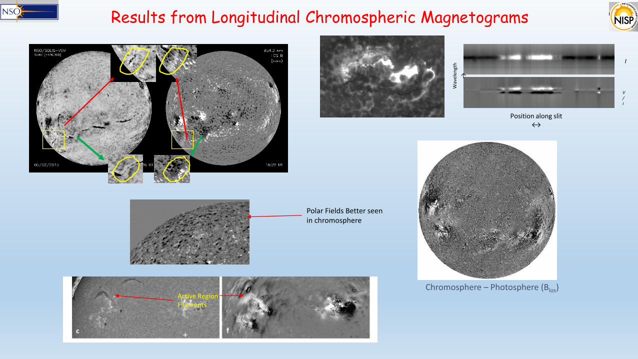
Chromosphere – Photosphere (Blos)

Results from Longitudinal Chromospheric Magnetograms

Position along slit ↔

Wav

elen

gth

→

I

V/I

Polar Fields Better seen in chromosphere

Active Region FIlaments

Full Stokes vector measurements in chromospheric line Ca 8542Modulator Design

IFilter FLC1 WP1 FLC2 WP2 Spacer

0 deg 246 deg 30 deg 90 deg

3mm 2.2 mm 10mm 2.2 mm 10mm 19 mm

8542 Modulator Package Schematic

Laboratory testing of Modulator Package

Measurement of the modulation signal (asterisks)

for various known input polarization vectors, and a forward model fit from

known angles and retardances (black line).

Optimum polarimetricefficiency (~ 0.57 for Q,U,V, as in J. Carlos del Toro Iniesta, 2007)

can be achieved from the computed set of angles for FLC modulators and

fixed retarders.

• Modulator package assembled as a

stack with index matching compound.

• SOLIS/VSM was brought to lab. for

installation of new modulator and

calibration optics.

• Polarimeter Calibration unit was

upgraded with dual passband

prefilter for 8542 and 6302 lines.

• SOLIS/VSM is back to observing

site

• Full Stokes Ca 8542 observations

began in November 2015.

Full Stokes vector measurements in chromospheric line Ca 8542Modulator Assembly + Installation

Full Stokes Observations in Ca II 854.2 nmFirst Light Results

• Area scans of activity belts with SOLIS VSM

• Typical scan covering an active region , as shown on the left takes 5 minutes.

Solis VSM instrument parameters

Spectral Lines: Fe I 630.2 nm, Ca II 854.2 nmPolarimetry: Stokes I, Q, U , VSpatial Sampling: 1 arcsec/pixelField-of-view: Full diskCadence: 22/45 min. for fulldisk (photo./chromo.)Active Region Mode: Typical AR scan in 3-5 minutes.Spectral Dispersion: Ca II (35 mA/pix), Fe I (25 mA/pix)

Inference of Chromospheric Vector Field

For full treatment of Stokes profiles we use NLTE inversion code NICOLE.

(Socas-Navarro et al, 2015, A&A)

“Our results indicate that the Ca II 8542 Å line is mostly sensitive to the layers enclosed in the range log τ = [0, −5.5], under the physical conditions that are present in our model atmospheres.”

(Quintero Noda et al., 2016, MNRAS)

UmbraNICOLE Inversions

PenumbraNICOLE Inversions

“Light-Bridge”

NICOLE Inversions

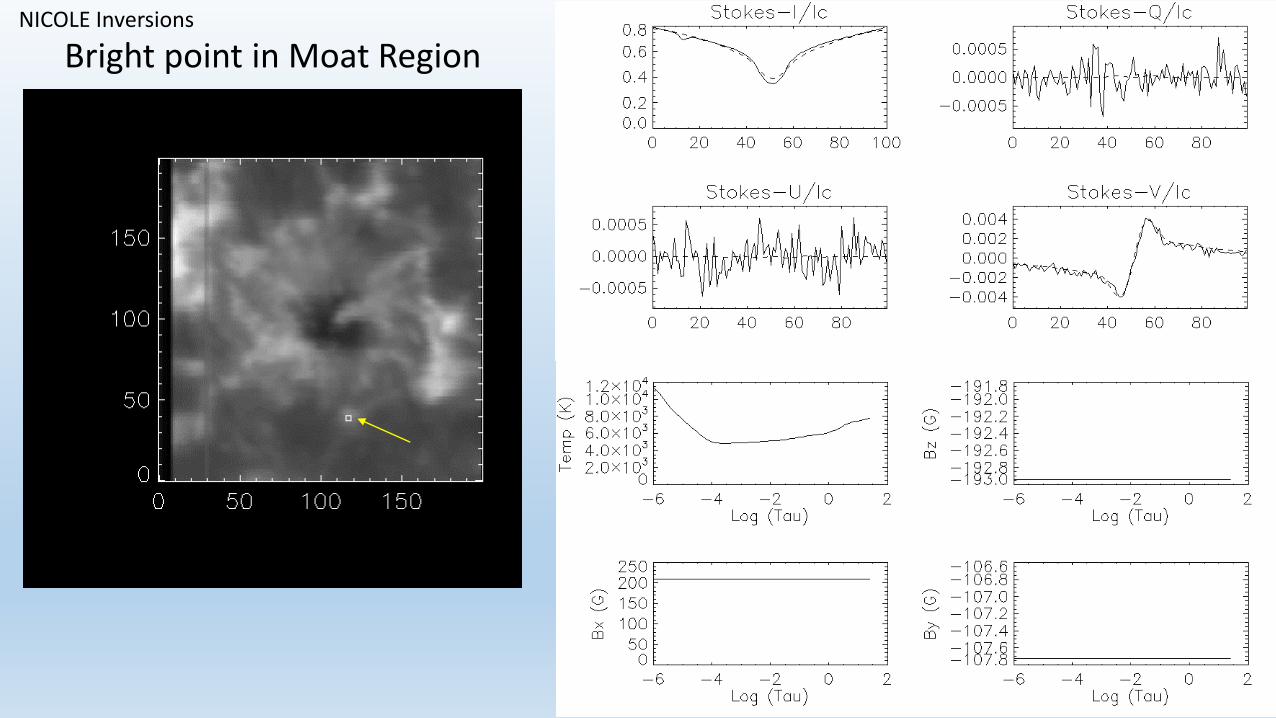
Bright point in Moat RegionNICOLE Inversions

PlageNICOLE Inversions

Maps of Magnetic and Velocity FieldNICOLE Inversions

Sample NICOLE Inversions for a Sunspot

Sample NICOLE Inversions for a Sunspot

Sample NICOLE Inversions for an Active Region

Can we recover Bz-gradient in solar atmosphere?

1

2

Future plansBetter Initialization:

• Weak Field Approx. can be used to initialize B-field.

• Inversions with binned set can be used as guess for full resolution

Faster Speed:

• More processors, GPUs ?

• Binning in spectral dimension.

Test Force-freeness:

• Test force-freeness compared to Photosphere

• Use as lower boundary condition for force-free extrapolations.

Multi-line Inversion:

Invert together with Fe I 630 nm lines to infer field gradients in stable sunspots.

(Fe and Ca lines are not observed simultaneously.)

Thanks!!