Induced Magnetic Fields in Solar System Bodies · Induced Magnetic Fields in Solar System Bodies...

Space Sci Rev (2010) 152: 391–421DOI 10.1007/s11214-009-9581-y

Induced Magnetic Fields in Solar System Bodies

Joachim Saur · Fritz M. Neubauer ·Karl-Heinz Glassmeier

Received: 5 April 2009 / Accepted: 12 October 2009 / Published online: 12 December 2009© The Author(s) 2009

Abstract Electromagnetic induction is a powerful technique to study the electrical con-ductivity of the interior of the Earth and other solar system bodies. Information about theelectrical conductivity structure can provide strong constraints on the associated internalcomposition of planetary bodies. Here we give a review of the basic principles of the elec-tromagnetic induction technique and discuss its application to various bodies of our solarsystem. We also show that the plasma environment, in which the bodies are embedded, gen-erates in addition to the induced magnetic fields competing plasma magnetic fields. Thesefields need to be treated appropriately to reliably interpret magnetic field measurements inthe vicinity of solar system bodies. Induction measurements are particularly important inthe search for liquid water outside of Earth. Magnetic field measurements by the Galileospacecraft provide strong evidence for a subsurface ocean on Europa and Callisto. The in-duction technique will provide additional important constraints on the possible subsurfacewater, when used on future Europa and Ganymede orbiters. It can also be applied to probeEnceladus and Titan with Cassini and future spacecraft.

Keywords Electromagnetic induction · Magnetic fields · Solar system bodies

1 Motivation and Background

The value of the electrical conductivity in naturally occurring matter varies enormously bymore than 20 orders of magnitude from highly conductive metals to nearly perfect isolators.

J. Saur (�) · F.M. NeubauerInstitut für Geophysik und Meteorologie, Universität zu Köln, Albertus-Magnus-Platz, 50923 Cologne,Germanye-mail: [email protected]

K.-H. GlassmeierInstitut für Geophysik und extraterrestrische Physik, TU Braunschweig, 38106 Braunschweig, Germany

K.-H. GlassmeierMax Planck Institut für Sonnensystemforschung, Max-Planck-Strasse 2, 37191 Katlenburg-Lindau,Germany

mailto:[email protected]

392 J. Saur et al.

Measurements of the electrical conductivity can thus be discriminative and well suited tocharacterize properties and spatial structures of matter in general or planetary bodies in ourcase. Knowledge of the electrical conductivity combined with cosmo-chemical, geological,gravitational and other geophysical information provides strong constraints on the structureof planetary bodies.

The change of magnetic flux through a conductor or the motion of a conductor througha magnetic field generates electric fields and thus also electric currents in the conductor.The changing electric fields and the electric currents are the source of secondary magneticfields, also called induced magnetic fields. The primary time variable magnetic fields arecalled inducing magnetic fields. Studies of the inducing and induced magnetic fields arethe core principle of the induction technique, through which the electrical conductivity canbe determined or constrained. This technique finds also ample application in engineeringand day-to-day experience. Each time we pass airport security, temporally changing electro-magnetic fields are exposed upon us. Possession of significantly conducting objects, such asmetal devices, generate secondary, i.e., induced magnetic fields. Airport security measuresthe secondary magnetic fields as their diagnostic means for metal objects.

Note, if we refer to induced magnetic fields, we refer to the aforementioned electromag-netic induction process, but not to a change of the magnetic induction B due to magnetizationM of matter. In the latter case the magnetic field strength H is modified by changes in themagnetic susceptibility χm such that B = μ0(H + M) = μ0(1 + χm)H = μrμ0H. For dia-magnetic and paramagnetic materials the relative magnetic permeability μr is close to unityand χm ≈ 0. This even holds in crustal layers of the Earth with ferromagnetic constituents. Itis also a good assumption in metallic cores of planetary bodies with temperatures above theCurie temperature. In this paper we consequently assume μ ≈ μ0. Also note, in accordancewith standard practice in the literature, in this chapter we refer to B as magnetic field, eventhough its is technically labeled magnetic induction.

The electromagnetic induction technique is a well developed and established method atEarth. It is extensively applied to study the electrical conductivity of the Earth at differentscales. The induction technique uses magnetic field measurements (and sometimes also elec-tric field measurements) obtained on the Earth’s surface or from satellites such as Magsat,Ørsted, and Champ. Time variable inducing magnetic fields are either naturally provided bytime dependent effects in the Earth’s ionosphere and magnetosphere or man made, for exam-ple, by transmitters particularly developed for the induction method or by low-frequency ra-dio waves operated for communications, but used by geophysicists for measuring inductiveresponses. The scales which are studied in geophysics by the induction technique vary fromglobal scales to study the Earth’s crust and parts of the Earth’s mantle to small scale objectsdown to dimensions of meters and less, e.g., water pipes, aquifers, waste sites, brines. Infor-mation on the spatial conductivity distribution provides in general constraints on chemicalcomposition and temperature. The induction technique at Earth is well developed and ma-ture at all fronts, i.e., in its physical and theoretical understanding, its technical applications,its numerical analysis of the measured data, as well as its associated geological interpreta-tion of the derived electrical conductivities. Not surprisingly, also a gigantic set of scientificreferences exists in this field, which can be tapped into by the planetary community (e.g.,Parkinson 1983; Schmucker 1985; Olsen 1999; Constable and Constable 2004). Applyingthe induction technique to other solar system bodies is in its infancy compared to the levelof sophistication reached at Earth. However, the induction technique applied to solar systembodies is often faced with new challenges not common at Earth and to be discussed in thischapter.

Induced Magnetic Fields in Solar System Bodies 393

The general aim in the application of the induction technique to solar system bodies is todetermine the conductivity structure of their interior. One of the key drivers for this applica-tion is the search for liquid water in our solar system. Liquid water is considered to be oneof the few essential building blocks for life as we know it. Surface layers of several plan-etary bodies in the outer solar system consist of frozen water with the possibility of liquidwater under the ice crust due to internal heating. Such subsurface liquid water layers underan ice crust also exist at Earth under the Antarctic ice, e.g. Lake Vostok and at least 145smaller lakes in the same region (e.g., Siegert et al. 2001, 2005). Frozen and liquid waterhave nearly the same density and thus cannot be distinguished directly by gravity measure-ments. However the electrical conductivity between frozen water and liquid saline waterdiffers by several orders of magnitude making the induction technique suitable for distinc-tion. The induction method finds also application in the study of other planetary properties,e.g. the existence and properties of a metallic core, which is e.g. uncertain in the case of theEarth moon.

In Sect. 2 we summarize some basic physical principles of the induction technique andalso discuss particular challenges this technique meets at solar system bodies. In the sub-sequent sections we then give a guided tour of solar system objects where induction playsa role. Particular emphasise is given to Jupiter’s satellite Europa, where the induction tech-nique is, arguably, further developed than for any other solar system body, with the exceptionof Earth.

2 Basic Theory: Earth and New Problems at Planetary Bodies

Before we discuss the state of the art of induction at planetary bodies, we repeat some ofthe basic theory of induction, which has been developed historically for the Earth. We beginwith the underlying equations for induction in a solid state or a conductive fluid at rest(Sect. 2.1) and then focus on induction for spherical geometry (Sect. 2.2). Afterwards wegeneralize the description of induction to a moving conductive fluid (Sect. 2.3).

2.1 Basic Equations

The fundamental equation to describe the induction process in a solid state body or in aconductive fluid at rest is the induction equation in a material with electrical conductivity σ

∂B∂t

= −∇ ×(

1

σμ0∇ × B

)(1)

which reads for constant conductivity

∂B∂t

= 1

σμ0ΔB. (2)

These equations can be derived from Maxwell’s equations and the simplest form of theisotropic Ohm’s law

j = σE (3)

for the electric current density j and the electric field E. In the derivation of (1) and (2),we retain the conductive currents (3), but neglect the displacement current in Ampere’s

394 J. Saur et al.

law. With this assumption, the magnetic field diffuses into the conductive material ratherthan propagates into it. This assumption holds if the time scales of the temporal variationexpressed by a frequency ω obey

ω � σμ0c2 (4)

with c the speed of light. Assuming a characteristic time scale of one minute, this conditionsis fulfilled if the conductivity is larger than ∼10−12 S m−1. This is well fulfilled for anyknown natural object in the solar system. Most time scales under consideration at solarsystem bodies are even longer than one minute. In the derivation of (2) it is also assumedthat the magnetic permeability μ can be approximated by μ0 (see Sect. 1).

Useful time and length scales for characterization of the induction process for objects ofsize L are the diffusion time

Tdiff = σμ0L2 (5)

and the frequency dependent skin depth

δ(ω) =√

2

σμ0ω≈ 1

2

√ρT km (6)

with the resistivity ρ = 1/σ and the period T = 2π/ω. The last term on the right-hand sidein (6) holds for SI-units and approximates the skin depth in km.

Since the induction equation is linear, we can decompose the time dependent primaryinducing magnetic field B(x, t) as a superposition of the real parts of fields with individualfrequencies ω in the form

B(x, t) = B̃(x)eiωt . (7)

Substituting (7) into (2) and introducing the complex wave vector k = ±(1 + i)√

μ0σω/2yields the Helmholtz equation

k2B̃(x) = ΔB̃(x). (8)

2.2 Induction in Spherical Geometry

The induction equation (2) is a linear parabolic partial differential equation. Well devel-oped tools for its solution exist in mathematical physics. In spherical coordinates it has beensolved on various levels of complexity for spherical distributions of the electrical conductiv-ity (e.g., Lahiri and Price 1939; Rikitake 1966; Parkinson 1983). In this subsection, we willdiscuss several solutions for spherical geometry.

2.2.1 Limit of Nearly Infinite Conductivity Case

One of the most simple solutions and in several cases already a very useful first order de-scription for some planetary satellites is given in the case when the conductivity and thethickness of the conducting shell D are large enough and the period T of the inducing fieldis small enough to obey the inequality (Neubauer 1999; Kivelson et al. 1999)

(δ/D)2 = 1

π(T /Tdiff)

2 � 1. (9)


In this case, the planetary body acts like a superconductor and time variable componentsobeying (9) are excluded from the conducting sphere by surface currents just inside thesurface of the sphere. For real superconductors this effect is called the Meissner–Ochsenfeldeffect and holds for any frequency ω. For non-superconductors in contrast, steady-state orvery low-frequency fields with ω = 2π/T → 0 can fully penetrate the conductor.

In case the external time-varying inducing field B0(t) is spatially homogeneous and inthe limit of nearly infinite conductivity σ → ∞, the induced, i.e. the secondary, field is adipole magnetic field

B∞ind(t) = μ0

4π

(3(r · M(t)

)r − r2M(t)

)/r5 (10)

with

M(t) = −2π

μ0B0(t)r

30 (11)

and the outer radius r0 of the conducting sphere or shell.

2.2.2 Single Layer with Finite Conductance

A very useful and still fairly easy to handle model is the single shell model with a con-stant conductivity (Lahiri and Price 1939; Parkinson 1983; Zimmer et al. 2000). We assumeone shell with conductivity σ , outer radius r0 and inner radius r1. The conductivity is zeroeverywhere else inside the planetary body of radius R.

Now we further assume that the exterior inducing field can be written as a poten-tial field B0 = −∇Ue . This holds in regions with negligible electric current, i.e. when∇ × B = μ0j = 0. The planetary bodies under considerations in this paper generally consistof poorly conductive surface layers. In these cases the potential representation is valid on andwithin the surface layers of the planetary bodies. The potential field can then be expandedinto spherical harmonics Sm

n (Θ,φ), with colatitude Θ and longitude φ (Rikitake 1966;Parkinson 1983; Olsen et al. 2009). If the conductivity distribution is radially symmet-ric, the resulting induced fields and its associated potentials U

n,mi are of the same degree

n and order m as the inducing field and its associated potentials Un,me (Parkinson 1983;

Schmucker 1985). This largely simplifies the analysis. For most planetary bodies radial sym-metry of the electrical conductivity is a reasonable first order assumption, and we can there-fore consider the inducing potential of a particular n and m without any loss of generality asthe real part of

Un,me = RBe

(r

R

)n

Smn (Θ,φ)eiωt (12)

with the complex coefficient Be. The full magnetic potential U = Ui + Ue is a linear super-position of all contributions of degree n and order m and of all frequencies ω. The inducingfields can be of varying nature for planetary bodies, e.g. spatially constant or inhomoge-neous. It can be also both, periodic and aperiodic. An aperiodic inducing signal can still beformally approximated in a temporally limited interval by a Fourier superposition in fre-quency space. We will discuss these effects in the following chapter where we cover theplanetary bodies individually.

The induction equation (2) must be solved inside the shell and also outside the shellsubject to the following boundary conditions for the total time-varying field: (i) B must be

396 J. Saur et al.

continuous across the boundaries of each shell. The normal component is continuous, andthe tangential component is continuous for the assumption μ = μ0 (see Sect. 1). (ii) B mustnot be infinite at the center of the body, r = 0, and (iii) B must be asymptotically equal tothe external field far away from the body (r R).

The total potential Un,m outside of the shell is the potential of the inducing Un,me and

the induced fields Un,mi for frequency ω and spherical harmonics Sm

n , characterized by thecomplex coefficients Be and Bi

Un,m = r0

(Be

(r

r0

)n

+ Bi

(r0

r

)n+1)Sm

n (Θ,φ)eiωt . (13)

The solution of (2) or (8) inside the conducting shell only contains poloidal magneticfields which can be described as a sum of the product of Bessel functions for the radial de-pendence with spherical harmonics for the longitudinal and latitudinal dependence (Rikitake1966; Parkinson 1983). Application of the boundary conditions (i) to (iii) at the inner andouter parts of the shell constrains the ratio of the complex amplitudes of the inducing to theinduced field to

Bi

Be

= −(

n

n + 1

)ξJn+3/2(r0k) − J−n−3/2(r0k)

ξJn−1/2(r0k) − J−n+1/2(r0k)(14)

with

ξ = (r1k)J−n−3/2(r1k)

(2n + 1)Jn+1/2(r1k) − (r1k)Jn−1/2(r1k). (15)

Jm are the Bessel function of first kind and order m. Zimmer et al. (2000) derived a similarsolution under the simplifying assumption that the inducing field is spatially homogeneous,i.e., n = 1.

The real and imaginary part of Bi/Be = A exp(iΦ) provide the amplitude A and thephase Φ so that the induced field outside of the planetary body is related to the induced fieldof a perfectly conducting sphere (see (10))

Bind(t) = AeiΦB∞ind(t) = AB∞

ind

(t + Φ

ω

). (16)

For finite conductivity the induced field is weaker than the primary field and its phase lagsthe primary inducing field, i.e. A < 1 and −π/2 ≤ Φ < 0. Note, A is calculated here atthe surface of the conducting shell r0 and not at the surface of the satellite R. For sphericalsymmetric conductivities, which is a premise for (12), an external inducing field n = 1, i.e.a spatially constant field, induces a dipole field.

In geophysics, several methods have been developed to describe the geomagnetic vari-ations at Earth, i.e. the inductive response of the Earth’s conductive layers to temporallychanging magnetic fields in the Earth’s ionosphere and magnetosphere (Schmucker 1985).One of these methods compares similar to the mathematical procedure of (12) to (15) theratio of the internal, i.e. induced, and external, i.e. inducing, parts of the magnetic poten-tials. This ratio is commonly called in geophysics the Q-response function and is a fre-quency dependent transfer function that connects the internal and the external coefficientsof the field expansion in spherical harmonics of order n (Schmucker 1985; Olsen 1999;Constable and Constable 2004):

Qn(ω) ≡ ιmn

εmn

= gmn − ihm

n

qmn − ism

n

= Bi

Be

(17)


where ιmn = gmn − ihm

n are the internal, and εmn = qm

n − ismn are the external potential coeffi-

cients. For more details on the complex notation of the magnetic potential and its coefficientssee chapter by Olsen et al. (2009) in this issue.

Attempts to estimate the conductivity profile as a function of depth at Earth based onsatellite observations, so far, rely on the assumption that the external (inducing) source is ofmagnetospheric origin with a spatial structure dominated by the spherical harmonics S0

1 , i.e.a spatially constant but time-varying field (Olsen 1999; Constable and Constable 2004). Inthe absence of currents at satellite altitude and after removal of other contributions, such asthe dynamo field from the core, the crustal and ionospheric magnetic fields, the remainingfield can simply be written as the potential

U 1,0(t) = r0

[ι01(t)

(r0

r

)2

+ ε01(t)

(r

r0

)]S0

1 (Θ). (18)

According to Gauss, the observed fields can then be separated in external (ε) and internal (ι)parts. Fourier transformation of the coefficients ε(t) and ι(t) into frequency space ω rendersthe frequency dependent transfer function Q1(ω). Constable and Constable (2004), for ex-ample, use corresponding periods from less than one day up to roughly 0.4 year. With inver-sion techniques subsequently, models of the conductivity-depth profile can be constructedbased on Q1(ω) (Olsen 1999; Constable and Constable 2004).

2.2.3 Induction in Sphere with Multi-layered Conductivity

In the previous subsection a single shell with finite conductivity was assumed. The solutioncan be extended to multiple layers with constant conductivities in each shell. The solutionof (2) in each shell together with the boundary conditions (i) to (iii) lead to recursive formulafound by Srivastava (1966). Schilling et al. (2007) derive a solution for a three layer modelrepresenting Europa’s ocean, mantle and core. Models with non constant conductivity dateback to as early as Lahiri and Price (1939) who assumed a conductivity increasing with aninverse power law of the radial distance from the center of the Earth.

2.3 Role of a Dynamic Plasma Environment

Solar system bodies are generally embedded in a dynamically changing magneto-plasma.All magnetic field measurements (except for the Earth and the Moon) have been performedin the past (and will still be performed in the foreseeable future) during satellite flybys orfrom satellites in orbit. In cases where the objects do not possess a substantial atmosphere(such as Europa, Ganymede, Callisto, or Enceladus), the objects are usually fully surroundedby plasma starting at the surface of the bodies. In other cases where objects possess a sub-stantial atmosphere (such as Titan), no plasma reaches the objects surfaces. In all thesecases the measurements are still gathered (above the surface or above the lower atmosphere)in a plasma environment which often contains significant electric current. Therefore themagnetic field cannot be written as a potential field and the separation in internal and exter-nal contributions as developed by Gauss (see chapter by Olsen et al. 2009) is not possibleany more and new approaches need to be developed. The following approach is based onSchilling et al. (2007, 2008).

Plasma effects and their associated electric currents, e.g. in the satellites’ ionospheres orAlfvén wings, cause strong magnetic field perturbations which can be equal or larger thanthe internally induced fields. In the analysis of magnetic field measurements to determine

398 J. Saur et al.

internally induced fields, the external fields therefore cannot be neglected. The external cur-rents close to the satellites can additionally be time variable and can contribute to inductionas well, while induction, vice versa, can modify the plasma flow and magnetic fields outsideof the planetary object.

The magnetic field in a plasma or within an electrically conductive fluid, cannot be de-scribed by an induction equation for solid state matter of the form (2) based on Ohm’slaw (3). In particular, the plasma velocity v with respect to the planetary objects introducesa motional electric field which changes Ohm’s law to

j = σ(E + v × B + Tadd). (19)

In a plasma Ohm’s law is in general quite complex (e.g., Baumjohann and Treumann 1996)and outside the realm of this chapter. Any additional terms in Ohm’s law are representedin (19) in the term Tadd. Their nature and relative importance depend on the particular plasmaphysical environment around the planetary object. The conductivity σ in (19) is in the sim-plest case isotropic and can, e.g., be due to the conductivity of the object’s ionosphere.Together with Faraday’s induction law, (19) leads to an induction equation of the form

∂B∂t

= ∇ × (v × B) − ∇ × (η∇ × B − Tadd) (20)

with the magnetic diffusivity η = 1/(μ0σ). Note, (20), reduces to (1) inside a non-movingpart of a planetary body where v = 0. No measurements of the fluid velocities in possible,conductive subsurface oceans exist. But the velocities are assumed to be small and to onlyweakly contribute to the exterior magnetic field. For example, Tyler (2008) discusses veloc-ities of less than 1 m/s within Europa’s possible ocean. Ocean tides at Earth generate smallpoloidal fields of the order of 1–10 nT, which can be observed from space and allow mon-itoring of the ocean flows (Tyler et al. 2003). Flows of extraterrestrial conductive oceansmight similarly be sounded through their induced magnetic fields.

To comprehensibly describe the magnetic field in the vicinity of a planetary body, theinduction equation (2) in the interior and the induction equation (20) for a plasma in theexterior need to be solved simultaneously. When the interior of a planetary body is liquidand moves with appreciable velocity v, then an induction equation of the form in (20) needsto be solved in the interior as well. In addition, the plasma momentum equation together withthe continuity and the energy equations in the exterior need to be solved self-consistently aswell. The plasma environment can in principal also be described by non-fluid models, suchas hybrid or full kinetic models. Due to the highly non-linear nature of these sets of plasmaequations, they can be solved in their full extent only numerically. A straightforward, butin most cases unfeasible procedure would be to self-consistently solve the plasma equationsand the induction equation inside and outside of the planetary body. The difficulty stemsfrom the different time scales of the processes, which will make simulations unrealisticallylong.

The magnetic field

B(x) = ⟨B(x)

⟩ + δB(x, t) (21)

consists in general of a time independent 〈B(x)〉 and a time dependent component δB(x, t).For a better understanding of the interaction in between the different processes that generatemagnetic field in this complex environment, as well for laying out a framework how to


numerically solve the set of equations, it is useful to decompose the magnetic field B intodifferent components:

B = B0 + BP + δBind(δB0) + δBind(δBP ). (22)

B0 is the component of an external background field, e.g. the magnetic field of a planetarymagnetosphere that surrounds a planetary moon at some distance from it. The second contri-bution is the magnetic field BP produced by plasma processes close to the body, e.g. throughthe currents in the bodies ionospheres or Alfvén wings. The third and fourth contributionsare the internally induced magnetic field δBind(δB0), δBind(δBP ) due to the time-varyingexternal background field δB0 and due to the time-varying plasma fields δBP , respectively.The induced fields δBind(δB0) and δBind(δBP ) are potential fields outside of the planetarybody, and the magnetospheric field B0 can usually be approximated by a potential field nearthe satellites as well.

With the aim to use induction to study properties of the planetary interior, the fields dueto the external plasma interaction BP + δBind(δBP ) can be considered a systematic measure-ment error that needs to be considered. In the absence of a significant time-varying externallyinducing magnetic fields δB0 (such as in the Saturn system), induction signals δBind(δBP )

might be generated due to time variable plasma magnetic fields δBP . These time variableplasma magnetic fields can be, for example, at Enceladus due to temporal changes in itsplume activity, or at Titan a result of an eclipse or due to temporal variations in the conduc-tivity distribution of the ionosphere. In these latter cases, BP(t) + δBind(δBP ) changes frommeasurement error to measurement target, and BP(t) + δBind(δBP ) establishes a possibilityfor the usage of the induction technique.

In cases of the Jovian and many other satellites, fortunately, the time scales that controlthe plasma in the exterior and the induction in the interior separate (Neubauer 1998). Thetime scale that controls the plasma interaction are on the order of minutes, while the timescales for induction are on the order of the planetary rotation period. Thus the planetaryinduction field can be considered quasi-stationary on time scales of the plasma interaction.But the plasma interaction reaches a quasi steady state as well on these time scales. Theplasma interaction during one planetary rotation can therefore be described by a consecutiveset of quasi-stationary plasma states during which the induction field is quasi-stationary aswell.

If the primary, inducing field is due to planetary rotation, the following iterative proce-dure to self-consistently solve the induction equation in the interior and exterior togetherwith the other plasma equations in the exterior based on the separation of time scales mightbe applied:

(a) First, the time interval spanning one rotation period is divided into small subsets,during which the plasma interaction and the induction fields can be considered quasi steadystate, respectively. In each small subset, we then solve the plasma interaction in the exteriorincluding the induction magnetic fields due to the changing planetary magnetic field, i.e.we compute B0, BP and δBind(δB0). The latter expression is calculated with (14) and (15).These calculations result in a set of three-dimensional magnetic fields at different times, i.e.subsets, during one rotation period.

(b) In this set of plasma interactions models, we now calculate the temporally constantand the temporally varying magnetic field contributions for each point in space. The tem-porally constant field 〈B(x)〉 is the temporally averaged field over one rotation period. Thetemporally changing field δB(x, t) is the deviation from the averaged field (see (21)).

400 J. Saur et al.

(c) The total time variable fields δB(x, t) now also contain time variable plasma fields,which generate time variable plasma induced magnetic fields δBind(δBP ). These plasma in-duced fields are computed in this step of the iteration process. Therefore we represent thetime variable plasma field δBP as a potential field Ue (see (12)) at or just below the surfaceof the satellite (where a potential representation of the magnetic field is possible). Equa-tions (14) and (15) subsequently provide the plasma induced magnetic fields for given Ue .Note, the time variable plasma fields are highly inhomogeneous in contrast to the time vari-able planetary magnetic field near the satellites and thus higher order contributions n in thespherical expansions in (14) and (15) are important.

(d) In the next iteration step, we calculate similar to (a) the plasma interaction and itsassociated plasma magnetic field BP within each small quasi-steady-state subset, but we nowinclude, additionally to B0 and δBind(δB0), the plasma induced field δBind(δBP ) computedin the previous step (c).

This cycle of iterations (b) to (d) are repeated until convergence is reached, i.e. inductionand plasma interaction in each individual subset do not change from one iteration to the nextone any more.

The procedure described above can be called forward-modeling similar to the nomen-clature in applied geophysics. In forward-modeling, induction and the plasma interactionare self-consistently calculated for a given set of model parameters, which are here the con-ductivity structure in the satellite’s interior, and background plasma and neutral propertiesoutside. The results are compared with the observations. Then a series of such forward-models with different model parameters are carried out to find a parameter set that explainsthe observations best.

A new level of modeling will be to construct an inverse-model. In inverse-modeling thewhole forward-model is inverted to directly solve for the internal parameters, which providethe best, e.g. least mean square, fit to the measurements.

3 Moon

Next to the Earth, the Moon and probably Europa are the solar system bodies best understoodin terms of electromagnetic induction. As the Moon does not possess a global magnetic fieldgenerated by an active dynamo (Stevenson 2003), the interaction of the Moon with the inter-planetary medium is much different from the terrestrial case. The Moon is always immersedin the ever changing magnetized solar wind plasma or is passing through the magnetotailof the Earth. No major magnetosphere with internal electric currents is developing, whichimplies that the Moon is directly exposed to the time-varying, external magnetic field of thesolar wind except perhaps for regions with strong magnetic anomalies (Dyal et al. 1975).As expected of even a poorly conducting object, the electromagnetic response of the Moonto these temporal fluctuations of the interplanetary magnetic field and its motion throughthe magnetotail is non-vanishing. Numerous studies on this response were conducted (e.g.,Blank and Sill 1969; Sonett et al. 1971; Dyal and Parkin 1973; Vanyan and Egorov 1975;Sonett 1982). Thus only a short summary is given here to demonstrate the potential of in-duction studies once sufficient observations are available.

Observational conditions for lunar induction studies are still much better than for anyother solar system body, except Earth. Surface magnetic field measurements from the Apollolunar surface magnetometer (Dyal and Gordon 1973) allow a detailed comparison with mag-netic field measurements made onboard a spacecraft such as Explorer 35. A transfer function


H(f ) can be defined by

H(f ) · B0(f ) = B0(f ) + Bind(f ) (23)

where B0(f ) is the Fourier component at frequency f of the external, inducing field of solarwind or magnetospheric origin, and Bind the induced magnetic field. The ratio of induced toinducing field can be derived from actual observations at the Moon’s surface and onboardan orbiting spacecraft. It can be interpreted using the Lahiri–Price theory referred to above.For a single layer reaching from the lunar surface to a depth of half the lunar radius and witha conductance of σ = 10−2 S/m the transfer function at 10−4 Hz is about 1.4.

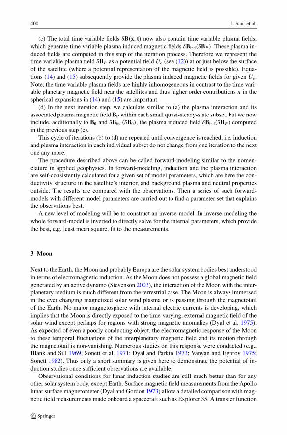
Hobbs et al. (1983) presented a detailed analysis of the available day-side magnetometerdata and derived the transfer function shown in Fig. 1. An apparent conductivity can bedetermined from the equation (e.g., Khan et al. 2006)

σa(f ) = 4H 2(f )

2πf μ0R2Moon

, (24)

where RMoon is the lunar radius. The frequency dependent skin depth (6) can be used to de-velop a depth sounding method. Low-frequency external field contributions penetrate deepinto the Moon and sound its deep structures, while higher frequency signals can only pen-etrate a short distance and thus sound only shallow structures. Therefore, this frequency

Fig. 1 A Lunar electromagnetictransfer function estimate and itsassociated apparent conductivitycurve, based on results of Hobbset al. (1983) (upper panel). Thebottom panel displays abest-effort electric conductivitymodel of the Moon as derived byHood et al. (1982)

402 J. Saur et al.

sounding allows a first view into the object under discussion. In case of the Moon the trans-fer function indicates an increasing electrical conductivity with depth.

However, further modeling and inversion efforts are necessary to infer the real conduc-tivity structure. The bottom panel of Fig. 1 shows the electrical conductivity structure ofthe Moon as a function of radial distance from its center derived by Hood et al. (1982).Upper and lower bounds for the conductivity are given. The conductivity was found to risefrom 10−4–10−3 S/m at a few hundred km depth to roughly 10−2 –1S/m at about 1100 kmdepth. The study by Hood et al. (1982) also allows for a metallic lunar core with a radiusof about 360 km and a conductivity σ > 102 S/m. Knowing the conductivity profile further-more enables one to constrain the compositional and thermal structure of the Moon (e.g.,Khan et al. 2006). Electromagnetic induction studies prove to be a powerful tool to studyplanetary interiors.

4 Mercury

Mercury is an enigmatic planet, also with respect to induction effects. The planetary mag-netic field is relatively weak with a current best estimate of its magnetic dipole moment ofM = −(230–290) nT (4π/μ0)R

3M , where RM = 2439 km is the Hermean planetary radius.

The negative sign denotes a polarity as for the current terrestrial dipole moment (Andersonet al. 2008). This weak magnetic field is nevertheless able to withstand the fast flowing solarwind plasma and generates a planetary magnetosphere first discovered by Ness et al. (1974).However, this magnetosphere is small with a mean planetocentric magnetopause stand-offdistance of only 1.7RM (Siscoe and Christopher 1975). Due to the small size of the magne-tosphere, which is filled by the planet to a large extent, surface magnetic fields of the orderof 100 nT generated by magnetopause currents are comparable to the dynamo generatedplanetary magnetic field of Mercury (e.g., Glassmeier et al. 2007b). As the magnetosphereis highly dynamic these large external fields cause major induction effects in the electricallyconducting planetary interior.

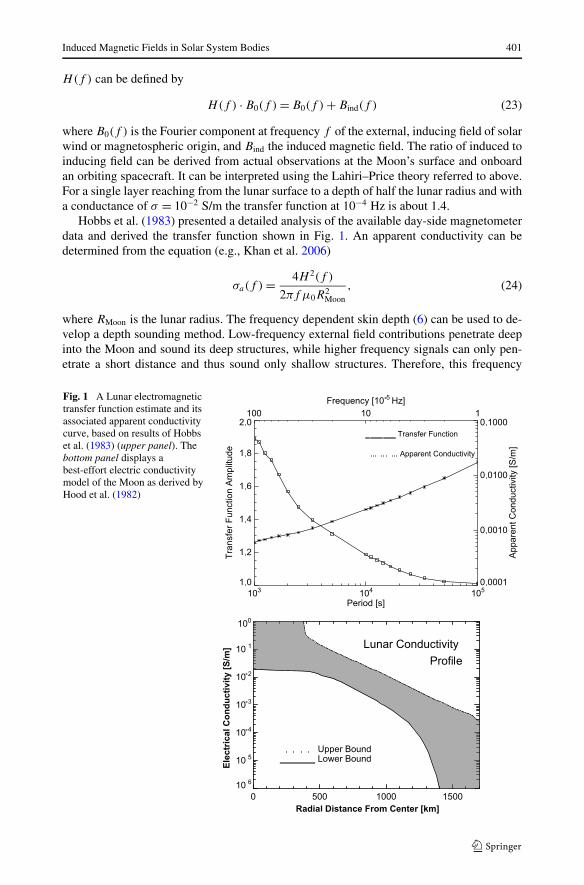
Already Hood and Schubert (1979) and Suess and Goldstein (1979) discussed such in-duction effects and pointed out that induction generated magnetic fields support the planetin withstanding the solar wind. A more detailed study on induction effects at Mercury waspresented by Grosser et al. (2004). Based on a potential field model of the magnetosphericmagnetic field following (Voigt 1981), assuming periodic variations of the magnetosphericsize and shape, and using the above outlined theoretical approach, especially (14), theyshowed that the induced magnetic field may well reach surface values of up to 20 nT, whichis about 10% of the dynamo generated magnetic field. As an example, Fig. 2 displays simu-lated magnetic field measurements made along a polar orbit around Mercury. The electricalconductivity distribution within the planet is spherically symmetric with a core conductivityof σ = 106 S/m. A core radius of 1860 km is assumed; the mantle is modeled as an electri-cally non-conductive shell. The magnetic field reaches a maximum value of 390 nT, out ofwhich about 290 nT are attributed to the dynamo generated field, 170 nT to magnetosphericcurrents, and about 20 nT to the induction effects.

The induced contribution, of course, depends on the assumed electrical conductivity dis-tribution. Not much is known about the actual conductivity distribution, but future magneticfield measurements at planet Mercury (Anderson et al. 2007; Glassmeier et al. 2009) willallow to constrain future models of the conductivity distribution.

Induction caused by temporal variations of the external magnetic field is not the onlyinduction effect of importance at Mercury. Not only a change of magnetic flux through a


Fig. 2 Modelled magnetic fieldmeasurements along an ellipticpolar orbit around Mercury(day-side periherm 1.15RM ,nightside apoherm 4RM ) (afterGrosser et al. 2004)

conductor causes induction, but also the motion of a conductor through a magnetic field.This situation is probably also realized at Mercury. Current Hermean dynamo models (e.g.,Wicht et al. 2007) assume a fluid planetary core. As this core is immersed in a large magneticfield of magnetospheric origin induction effects due to the relative motion of the conductivefluid to the field are to be expected. As a possible effect of the external field on the fluidGlassmeier et al. (2007a) and Heyner et al. (2009) study the inductive influence of the mag-netospheric field on the dynamo process in the planetary interior (described by an equationof the form (20) with a particular choice of Tadd and externally inducing magnetic field con-tributions, see (22)). As the external field, generated by the solar wind plasma-planetarymagnetic field interaction, is always directed anti-parallel to the dynamo generated dipolemoment a negative feedback is possible. A feedback dynamo is thus an interesting possibil-ity to explain the observed weak magnetic field at Mercury.

5 Jupiter’s Satellites

5.1 Basic Principle and the Nature of Inducing Fields

Jupiter’s large icy satellites Europa and Callisto are two of the few solar system objectswhere induction has been observed to take place (Khurana et al. 1998; Neubauer 1998;Kivelson et al. 2000). The third large icy satellite of Jupiter, Ganymede, shows hints ofinduction, which are however inconclusive (Kivelson et al. 2002). At Io no induction sig-natures have been observed. Io’s magnetic field environment is dominated by very strongplasma interaction fields compared to the other Galilean satellites (Kivelson et al. 2004;Saur et al. 2002).

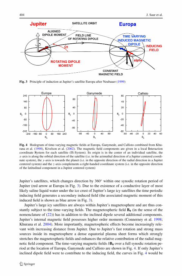
The induction is generated by a time periodic magnetic field, whose primary origin isthe inclination of Jupiter’s magnetic dipole moment with respect to Jupiter’s rotation axisby 9.6◦. The inclined magnetic moment rotates with Jupiter similar to the beacon of a lighthouse. The inclined moment can be decomposed in a component parallel and a componentperpendicular to the spin axis (see Fig. 3). The component parallel to the spin axis generatesa dipole magnetic field symmetric with respect to the rotation axis and thus does not producea time variable magnetic field. The component of the magnetic moment perpendicular tothe spin axis (red arrow at Jupiter in Fig. 3) generates a magnetic field at the locations of

404 J. Saur et al.

Fig. 3 Principle of induction at Jupiter’s satellite Europa after Neubauer (1999)

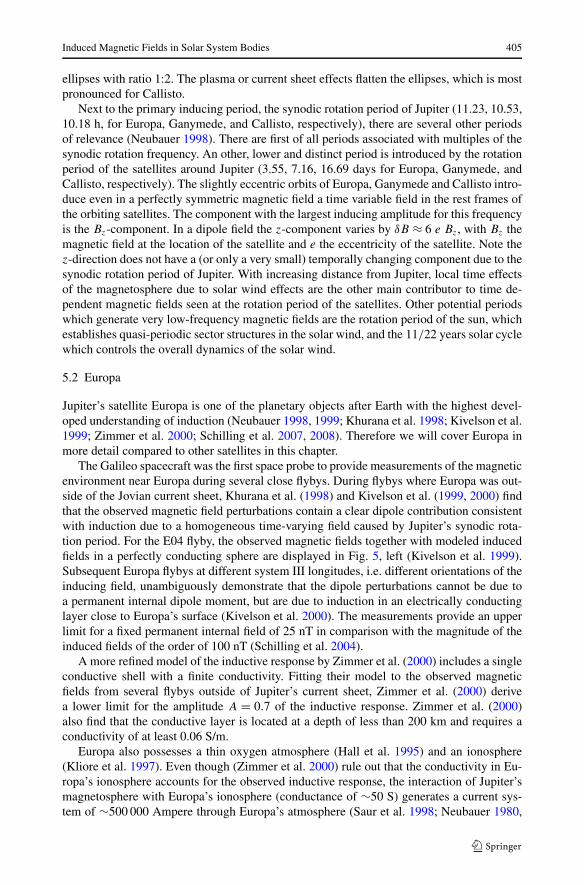
Fig. 4 Hodogram of time-varying magnetic fields at Europa, Ganymede, and Callisto combined from Khu-rana et al. (1998), Kivelson et al. (2002). The magnetic field components are given in a local Interactioncoordinate System for each satellite (IS-System). Its origin is in the center of an individual satellite, thex-axis is along the orbital direction of the satellite (i.e. in the azimuthal direction of a Jupiter centered coordi-nate system), the y-axis is towards the planet (i.e. in the opposite direction of the radial direction in a Jupitercentered system) and the z-axis complements a right-handed coordinate system (i.e. in the opposite directionof the latitudinal component in a Jupiter centered system)

Jupiter’s satellites, which changes direction by 360◦ within one synodic rotation period ofJupiter (red arrow at Europa in Fig. 3). Due to the existence of a conductive layer of mostlikely saline liquid water under the ice crust of Jupiter’s large icy satellites the time periodicinducing field generates a secondary induced field (the associated magnetic moment of thisinduced field is shown as blue arrow in Fig. 3).

Jupiter’s large icy satellites are always within Jupiter’s magnetosphere and are thus con-stantly subject to the time-varying fields. The magnetospheric field B0 (in the sense of thenomenclature of (22)) has in addition to the inclined dipole several additional components.Jupiter’s internal magnetic field possesses higher order moments (Connerney et al. 1998;Khurana et al. 2004). More importantly, magnetospheric effects become increasingly rele-vant with increasing distance from Jupiter. Due to Jupiter’s fast rotation and strong masssources inside its magnetosphere a dense equatorial plasma sheet forms which stronglystretches the magnetospheric fields and enhances the relative contribution of the radial mag-netic field component. The time-varying magnetic fields δB0 over a full synodic rotation pe-riod at the location of Europa, Ganymede and Callisto are shown in Fig. 4. If only Jupiter’sinclined dipole field were to contribute to the inducing field, the curves in Fig. 4 would be


ellipses with ratio 1:2. The plasma or current sheet effects flatten the ellipses, which is mostpronounced for Callisto.

Next to the primary inducing period, the synodic rotation period of Jupiter (11.23, 10.53,10.18 h, for Europa, Ganymede, and Callisto, respectively), there are several other periodsof relevance (Neubauer 1998). There are first of all periods associated with multiples of thesynodic rotation frequency. An other, lower and distinct period is introduced by the rotationperiod of the satellites around Jupiter (3.55, 7.16, 16.69 days for Europa, Ganymede, andCallisto, respectively). The slightly eccentric orbits of Europa, Ganymede and Callisto intro-duce even in a perfectly symmetric magnetic field a time variable field in the rest frames ofthe orbiting satellites. The component with the largest inducing amplitude for this frequencyis the Bz-component. In a dipole field the z-component varies by δB ≈ 6 e Bz, with Bz themagnetic field at the location of the satellite and e the eccentricity of the satellite. Note thez-direction does not have a (or only a very small) temporally changing component due to thesynodic rotation period of Jupiter. With increasing distance from Jupiter, local time effectsof the magnetosphere due to solar wind effects are the other main contributor to time de-pendent magnetic fields seen at the rotation period of the satellites. Other potential periodswhich generate very low-frequency magnetic fields are the rotation period of the sun, whichestablishes quasi-periodic sector structures in the solar wind, and the 11/22 years solar cyclewhich controls the overall dynamics of the solar wind.

5.2 Europa

Jupiter’s satellite Europa is one of the planetary objects after Earth with the highest devel-oped understanding of induction (Neubauer 1998, 1999; Khurana et al. 1998; Kivelson et al.1999; Zimmer et al. 2000; Schilling et al. 2007, 2008). Therefore we will cover Europa inmore detail compared to other satellites in this chapter.

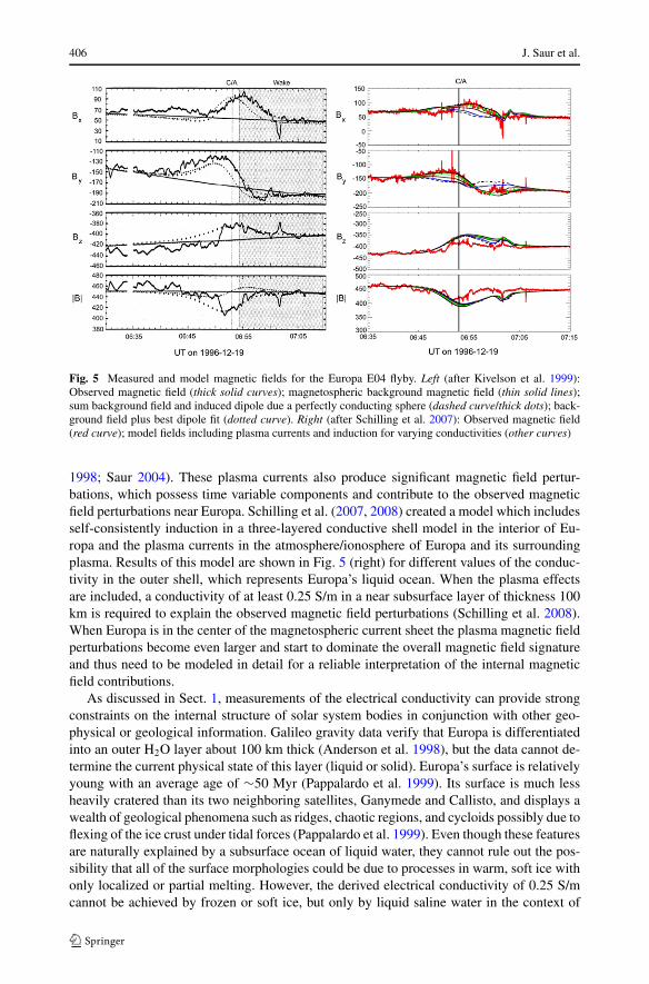
The Galileo spacecraft was the first space probe to provide measurements of the magneticenvironment near Europa during several close flybys. During flybys where Europa was out-side of the Jovian current sheet, Khurana et al. (1998) and Kivelson et al. (1999, 2000) findthat the observed magnetic field perturbations contain a clear dipole contribution consistentwith induction due to a homogeneous time-varying field caused by Jupiter’s synodic rota-tion period. For the E04 flyby, the observed magnetic fields together with modeled inducedfields in a perfectly conducting sphere are displayed in Fig. 5, left (Kivelson et al. 1999).Subsequent Europa flybys at different system III longitudes, i.e. different orientations of theinducing field, unambiguously demonstrate that the dipole perturbations cannot be due toa permanent internal dipole moment, but are due to induction in an electrically conductinglayer close to Europa’s surface (Kivelson et al. 2000). The measurements provide an upperlimit for a fixed permanent internal field of 25 nT in comparison with the magnitude of theinduced fields of the order of 100 nT (Schilling et al. 2004).

A more refined model of the inductive response by Zimmer et al. (2000) includes a singleconductive shell with a finite conductivity. Fitting their model to the observed magneticfields from several flybys outside of Jupiter’s current sheet, Zimmer et al. (2000) derivea lower limit for the amplitude A = 0.7 of the inductive response. Zimmer et al. (2000)also find that the conductive layer is located at a depth of less than 200 km and requires aconductivity of at least 0.06 S/m.

Europa also possesses a thin oxygen atmosphere (Hall et al. 1995) and an ionosphere(Kliore et al. 1997). Even though (Zimmer et al. 2000) rule out that the conductivity in Eu-ropa’s ionosphere accounts for the observed inductive response, the interaction of Jupiter’smagnetosphere with Europa’s ionosphere (conductance of ∼50 S) generates a current sys-tem of ∼500 000 Ampere through Europa’s atmosphere (Saur et al. 1998; Neubauer 1980,

406 J. Saur et al.

Fig. 5 Measured and model magnetic fields for the Europa E04 flyby. Left (after Kivelson et al. 1999):Observed magnetic field (thick solid curves); magnetospheric background magnetic field (thin solid lines);sum background field and induced dipole due a perfectly conducting sphere (dashed curve/thick dots); back-ground field plus best dipole fit (dotted curve). Right (after Schilling et al. 2007): Observed magnetic field(red curve); model fields including plasma currents and induction for varying conductivities (other curves)

1998; Saur 2004). These plasma currents also produce significant magnetic field pertur-bations, which possess time variable components and contribute to the observed magneticfield perturbations near Europa. Schilling et al. (2007, 2008) created a model which includesself-consistently induction in a three-layered conductive shell model in the interior of Eu-ropa and the plasma currents in the atmosphere/ionosphere of Europa and its surroundingplasma. Results of this model are shown in Fig. 5 (right) for different values of the conduc-tivity in the outer shell, which represents Europa’s liquid ocean. When the plasma effectsare included, a conductivity of at least 0.25 S/m in a near subsurface layer of thickness 100km is required to explain the observed magnetic field perturbations (Schilling et al. 2008).When Europa is in the center of the magnetospheric current sheet the plasma magnetic fieldperturbations become even larger and start to dominate the overall magnetic field signatureand thus need to be modeled in detail for a reliable interpretation of the internal magneticfield contributions.

As discussed in Sect. 1, measurements of the electrical conductivity can provide strongconstraints on the internal structure of solar system bodies in conjunction with other geo-physical or geological information. Galileo gravity data verify that Europa is differentiatedinto an outer H2O layer about 100 km thick (Anderson et al. 1998), but the data cannot de-termine the current physical state of this layer (liquid or solid). Europa’s surface is relativelyyoung with an average age of ∼50 Myr (Pappalardo et al. 1999). Its surface is much lessheavily cratered than its two neighboring satellites, Ganymede and Callisto, and displays awealth of geological phenomena such as ridges, chaotic regions, and cycloids possibly due toflexing of the ice crust under tidal forces (Pappalardo et al. 1999). Even though these featuresare naturally explained by a subsurface ocean of liquid water, they cannot rule out the pos-sibility that all of the surface morphologies could be due to processes in warm, soft ice withonly localized or partial melting. However, the derived electrical conductivity of 0.25 S/mcannot be achieved by frozen or soft ice, but only by liquid saline water in the context of


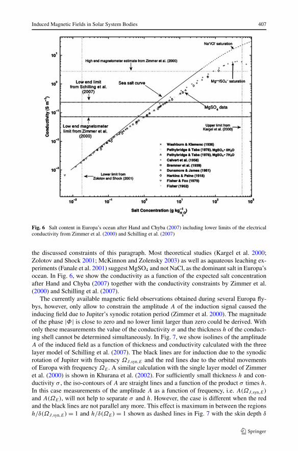
Fig. 6 Salt content in Europa’s ocean after Hand and Chyba (2007) including lower limits of the electricalconductivity from Zimmer et al. (2000) and Schilling et al. (2007)

the discussed constraints of this paragraph. Most theoretical studies (Kargel et al. 2000;Zolotov and Shock 2001; McKinnon and Zolensky 2003) as well as aquateous leaching ex-periments (Fanale et al. 2001) suggest MgSO4 and not NaCl, as the dominant salt in Europa’socean. In Fig. 6, we show the conductivity as a function of the expected salt concentrationafter Hand and Chyba (2007) together with the conductivity constraints by Zimmer et al.(2000) and Schilling et al. (2007).

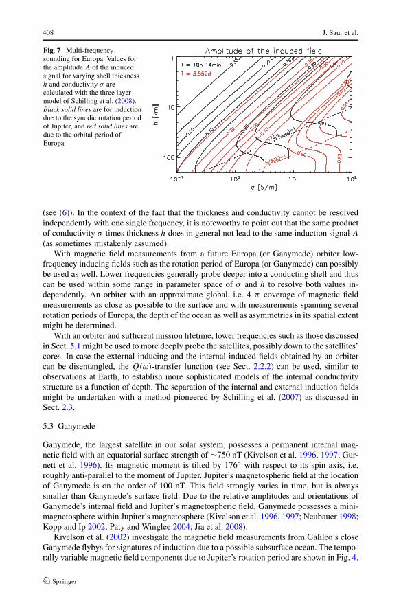
The currently available magnetic field observations obtained during several Europa fly-bys, however, only allow to constrain the amplitude A of the induction signal caused theinducing field due to Jupiter’s synodic rotation period (Zimmer et al. 2000). The magnitudeof the phase |Φ| is close to zero and no lower limit larger than zero could be derived. Withonly these measurements the value of the conductivity σ and the thickness h of the conduct-ing shell cannot be determined simultaneously. In Fig. 7, we show isolines of the amplitudeA of the induced field as a function of thickness and conductivity calculated with the threelayer model of Schilling et al. (2007). The black lines are for induction due to the synodicrotation of Jupiter with frequency ΩJ,syn,E and the red lines due to the orbital movementsof Europa with frequency ΩE . A similar calculation with the single layer model of Zimmeret al. (2000) is shown in Khurana et al. (2002). For sufficiently small thickness h and con-ductivity σ , the iso-contours of A are straight lines and a function of the product σ times h.In this case measurements of the amplitude A as a function of frequency, i.e. A(ΩJ,syn,E)

and A(ΩE), will not help to separate σ and h. However, the case is different when the redand the black lines are not parallel any more. This effect is maximum in between the regionsh/δ(ΩJ,syn,E) = 1 and h/δ(ΩE) = 1 shown as dashed lines in Fig. 7 with the skin depth δ

408 J. Saur et al.

Fig. 7 Multi-frequencysounding for Europa. Values forthe amplitude A of the inducedsignal for varying shell thicknessh and conductivity σ arecalculated with the three layermodel of Schilling et al. (2008).Black solid lines are for inductiondue to the synodic rotation periodof Jupiter, and red solid lines aredue to the orbital period ofEuropa

(see (6)). In the context of the fact that the thickness and conductivity cannot be resolvedindependently with one single frequency, it is noteworthy to point out that the same productof conductivity σ times thickness h does in general not lead to the same induction signal A

(as sometimes mistakenly assumed).With magnetic field measurements from a future Europa (or Ganymede) orbiter low-

frequency inducing fields such as the rotation period of Europa (or Ganymede) can possiblybe used as well. Lower frequencies generally probe deeper into a conducting shell and thuscan be used within some range in parameter space of σ and h to resolve both values in-dependently. An orbiter with an approximate global, i.e. 4 π coverage of magnetic fieldmeasurements as close as possible to the surface and with measurements spanning severalrotation periods of Europa, the depth of the ocean as well as asymmetries in its spatial extentmight be determined.

With an orbiter and sufficient mission lifetime, lower frequencies such as those discussedin Sect. 5.1 might be used to more deeply probe the satellites, possibly down to the satellites’cores. In case the external inducing and the internal induced fields obtained by an orbitercan be disentangled, the Q(ω)-transfer function (see Sect. 2.2.2) can be used, similar toobservations at Earth, to establish more sophisticated models of the internal conductivitystructure as a function of depth. The separation of the internal and external induction fieldsmight be undertaken with a method pioneered by Schilling et al. (2007) as discussed inSect. 2.3.

5.3 Ganymede

Ganymede, the largest satellite in our solar system, possesses a permanent internal mag-netic field with an equatorial surface strength of ∼750 nT (Kivelson et al. 1996, 1997; Gur-nett et al. 1996). Its magnetic moment is tilted by 176◦ with respect to its spin axis, i.e.roughly anti-parallel to the moment of Jupiter. Jupiter’s magnetospheric field at the locationof Ganymede is on the order of 100 nT. This field strongly varies in time, but is alwayssmaller than Ganymede’s surface field. Due to the relative amplitudes and orientations ofGanymede’s internal field and Jupiter’s magnetospheric field, Ganymede possesses a mini-magnetosphere within Jupiter’s magnetosphere (Kivelson et al. 1996, 1997; Neubauer 1998;Kopp and Ip 2002; Paty and Winglee 2004; Jia et al. 2008).

Kivelson et al. (2002) investigate the magnetic field measurements from Galileo’s closeGanymede flybys for signatures of induction due to a possible subsurface ocean. The tempo-rally variable magnetic field components due to Jupiter’s rotation period are shown in Fig. 4.


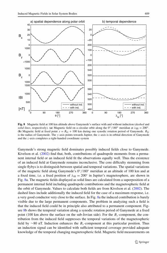
Fig. 8 Magnetic field at 100 km altitude above Ganymede’s surface with and without induction (dashed andsolid lines, respectively). (a) Magnetic field on a circular orbit along the 0◦/180◦ meridian at λIII = 200◦ .(b) Magnetic field at fixed point y = RG + 100 km during one synodic rotation period of Ganymede. RG

is the radius of Ganymede. The y-axis points towards Jupiter, the x-axis is in orbital direction of Ganymedeand the z-axis completes a right-handed coordinate system

Ganymede’s strong magnetic field dominates possibly induced fields close to Ganymede.Kivelson et al. (2002) find that, both, contributions of quadrupole moments from a perma-nent internal field or an induced field fit the observations equally well. Thus the existenceof an induced field at Ganymede remains inconclusive. The core difficulty stemming fromsingle flybys is to distinguish between spatial and temporal variations. The spatial variationsof the magnetic field along Ganymede’s 0◦/180◦ meridian at an altitude of 100 km and ata fixed time, i.e. a fixed position of λIII = 200◦ in Jupiter’s magnetosphere, are shown inFig. 8a. The magnetic fields displayed as solid lines are calculated from a superposition of apermanent internal field including quadrupole contributions and the magnetospheric field atthe orbit of Ganymede. Values to calculate both fields are from Kivelson et al. (2002). Thedashed lines include additionally the induced field for the case of a maximum response, i.e.a very good conductor very close to the surface. In Fig. 8a the induced contribution is barelyvisible due to the large permanent components. The problem in analyzing such a field isthat the induced field could be in principle also attributed to a permanent component. Fig-ure 8b shows the temporal variation along a synodic rotation period of Ganymede at a fixedpoint (100 km above the surface on the sub-Jovian side). For the By -component, the con-tribution from the induced field suppresses the temporal variations of the magnetosphericfield by ∼80 nT. Induction enhances the Bx -component at this particular position. Thusan induction signal can be identified with sufficient temporal coverage provided adequateknowledge of the temporal changing magnetospheric field. Magnetic field measurements on

410 J. Saur et al.

a future Ganymede orbiter will thus establish/rule out the existence of an induced field andthus help to settle the question of the existence of a subsurface ocean.

Similarly to Mercury, the very long period inducing fields at Ganymede may also beinvolved in the dynamo action in Ganymede.

5.4 Callisto

Callisto, the second largest of the Galilean satellites is only partially differentiated andposses the oldest surface of all Galilean satellites. It is heavily cratered and geologicallyinactive. Therefore it was quite surprising when the Galileo spacecraft magnetic fieldmeasurements near Callisto were observed to be consistent with induction possibly dueto a liquid subsurface ocean in Callisto’s interior (Neubauer 1998; Khurana et al. 1998;Kivelson et al. 1999; Zimmer et al. 2000). Near the orbit of Callisto, the radial componentof Jupiter’s magnetic field is the dominating time variable component (i.e. the By -componentin Fig. 4). It is directed outward or inward depending on whether Callisto is below or abovethe current sheet. For the cases when Callisto is outside of the current sheet, Zimmer et al.(2000) compared modeled induced magnetic fields from a single shell model to measure-ments by the Galileo spacecraft. The authors find that the conductivity in the model shellneeds to exceed 0.02 S/m at a depth of less than 300 km. The larger depth of the potentiallyassociated subsurface ocean compared to the smaller depth at Europa could be the reasonwhy Callisto’s surface is old and geological unaltered. An ocean much closer to the surface,as at Europa, will more strongly drive geological and tectonic near-surface processes.

6 Saturn’s Satellites

6.1 General

One of the major discoveries of the early Pioneer 11 and Voyager flyby missions to Sat-urn in 1979–1981 was the detection of a highly axisymmetric planetary magnetic field de-rived within the limitations of the flyby trajectories (Acuña and Ness 1980; Smith et al.1980). These results were confirmed by the analysis of the first Cassini magnetic field data(Dougherty et al. 2005).

At Saturn a small periodic planetary magnetic field portion with a period apparently nearthe probable rotational period of the planet’s interior has been observed mainly in the magne-tospheric Bϕ-component but also in the other components (Southwood and Kivelson 2007).The apparent periodicity is slowly varying in time but with a rate of change currently notvery well understood. In addition, the weak variation of the periodic field with distance fromSaturn seems not to be compatible with an internal origin (Espinosa and Dougherty 2000;Espinosa et al. 2003).The periodic field component is weak compared with the axisym-metric portion in the inner magnetosphere. With the definitions in (22) out to Rhea thecontribution of the magnetospheric field B0(t) to the inducing field Bi is then com-posed of periodic fields with ∼10 nT peak-to-peak amplitude (Giampieri et al. 2006;Southwood and Kivelson 2007) with a slowly varying period near ∼10.5 h and aperiodicfields due to internally and externally driven magnetospheric dynamics. In contrast to thesituation at Jupiter’s satellite Europa (Schilling et al. 2007) and also at Ganymede and Cal-listo, where the inducing fields are dominated by the time-varying magnetospheric com-ponent, the dominant sources of the inducing fields Bi at Saturn’s satellites Enceladus andTitan are the substantial temporal variations in their total plasma magnetic fields BP(t) de-fined as δBP(t) instead of the small magnetospheric contributions. This can be deduced from


model computations reported in the next sections on Enceladus and on Titan. Although theperiodic field component of magnetospheric origin is weak compared with the axisymmetricportion in the inner magnetosphere, it becomes comparable further out, i.e. at Titan’s orbit.However, at Titan it is not of much help because of Titan’s almost complete shielding by itsthick atmosphere- ionosphere system.

While the induction cases of Enceladus and Titan will be discussed in the next two Sub-sections in some detail, a few words on induction in the remaining satellites of Saturn seemto be warranted. No substantial atmosphere has been detected at these satellites. Thus in-ducing fields will not be modified noticeably by an atmosphere-ionosphere system, i.e.δBP(t) ≈ 0. The small inducing fields of magnetospheric origin out to Rhea have alreadybeen mentioned. Outside of Titan’s orbit only aperiodic fields are available for inductionstudies. A study of induction effects would require at least a carefully chosen sequence offlybys. Looking for possible targets for induction studies Rhea seems to be the best candidate(Hussmann et al. 2006) for the existence of an ocean. Finally, we mention for completenessthat permanent internal magnetic field components have not been seen at any of the Sat-urnian satellites.

6.2 Enceladus

After early hints for a geologically active interior of Enceladus by the Voyager imagingexperiment (Smith et al. 1982) an active gas plume above the southern polar region inter-acting strongly with the magnetospheric plasma was initially observed by the Cassini mag-netometer experiment (Dougherty et al. 2006). This was followed by important subsequentobservations and interpretations by remote sensing and in-situ experiments onboard Cassini(Porco et al. 2006; Hansen et al. 2006; Waite et al. 2006; Tokar et al. 2006). Although afull discussion of this interesting subject is outside the scope of this book, the followingpicture relevant for this section has emerged. The jets of mostly water vapor issue from lo-cations on the so-called “tiger stripes”, which are linear features in the southern polar regionof Enceladus. Several sources, which vary in time, have been identified. The origin of thewater vapor is still controversial between sublimation from internal clathrate surfaces andevaporation from the liquid–vapor interface in nozzle-like vents (Schmidt et al. 2008). Theenergy source is also not clear yet. In addition to water vapor the plumes contain gases likeCO2, CO or N2, CH4 etc. and ice particles which maintain the E-ring (Waite et al. 2006;Spahn et al. 2006). The composition of the partly contaminated ice and dust grains origi-nating at Enceladus suggest the water bodies below the surface of Enceladus are “contam-inated” by cations and anions due to leaching of the “rocky” part of the interior (Postberget al. 2009). This would then make them “visible” to electromagnetic induction studies. Thesame is true if an innermost rock-metal core of Enceladus were large and conductive enough.

Electromagnetic induction studies can thus be used to observationally investigate elec-trolytically conducting bodies of water ranging from a global ocean to a more localizedpond below the surface and possible a core of Enceladus, which are problems at the heart ofthe contemporary discussion of Enceladus’ interior and plume mechanisms. For these stud-ies sufficiently quickly varying inducing fields Bi (t) ∼ δBP (t) are necessary. The inducingfields Bi (t) drive induced fields Bind, which have to be separated from the inducing fieldin a proper analysis of the data. For a proper assessment, some information on the electri-cal conductivity would be helpful. With the only quantitative model of the chemistry of anocean below Enceladus’ surface, which is in contact with a rocky core, Zolotov (2007) hasobtained salinities up to 20 g/kg H2O, which is just below 35 g/kg H2O for the terrestrialocean. Thus except for differences in chemical composition we take the conductivity of the

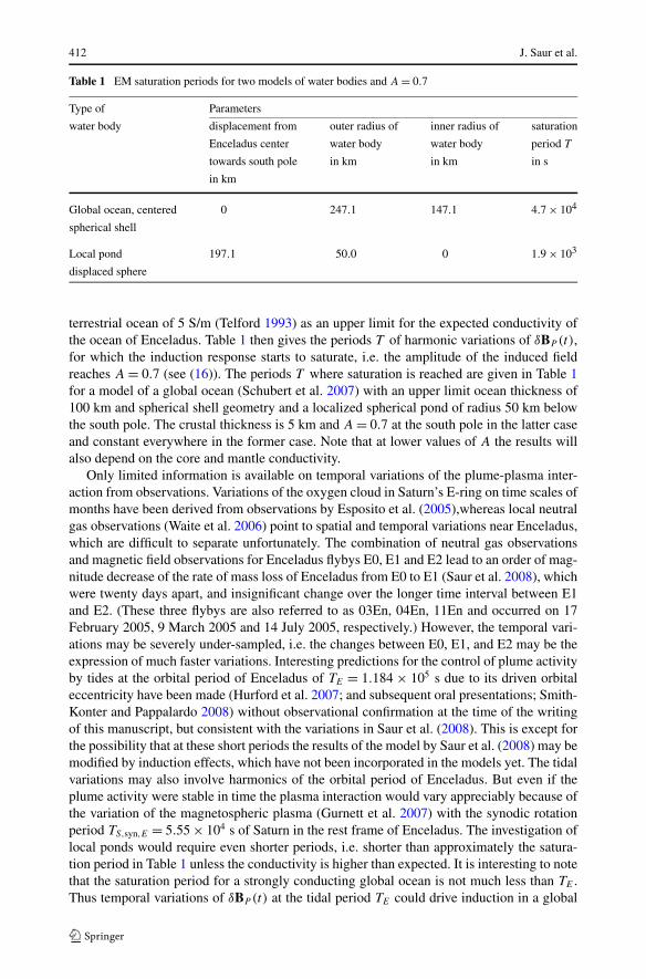
412 J. Saur et al.

Table 1 EM saturation periods for two models of water bodies and A = 0.7

Type of Parameters

water body displacement from outer radius of inner radius of saturation

Enceladus center water body water body period T

towards south pole in km in km in s

in km

Global ocean, centered 0 247.1 147.1 4.7 × 104

spherical shell

Local pond 197.1 50.0 0 1.9 × 103

displaced sphere

terrestrial ocean of 5 S/m (Telford 1993) as an upper limit for the expected conductivity ofthe ocean of Enceladus. Table 1 then gives the periods T of harmonic variations of δBP (t),for which the induction response starts to saturate, i.e. the amplitude of the induced fieldreaches A = 0.7 (see (16)). The periods T where saturation is reached are given in Table 1for a model of a global ocean (Schubert et al. 2007) with an upper limit ocean thickness of100 km and spherical shell geometry and a localized spherical pond of radius 50 km belowthe south pole. The crustal thickness is 5 km and A = 0.7 at the south pole in the latter caseand constant everywhere in the former case. Note that at lower values of A the results willalso depend on the core and mantle conductivity.

Only limited information is available on temporal variations of the plume-plasma inter-action from observations. Variations of the oxygen cloud in Saturn’s E-ring on time scales ofmonths have been derived from observations by Esposito et al. (2005),whereas local neutralgas observations (Waite et al. 2006) point to spatial and temporal variations near Enceladus,which are difficult to separate unfortunately. The combination of neutral gas observationsand magnetic field observations for Enceladus flybys E0, E1 and E2 lead to an order of mag-nitude decrease of the rate of mass loss of Enceladus from E0 to E1 (Saur et al. 2008), whichwere twenty days apart, and insignificant change over the longer time interval between E1and E2. (These three flybys are also referred to as 03En, 04En, 11En and occurred on 17February 2005, 9 March 2005 and 14 July 2005, respectively.) However, the temporal vari-ations may be severely under-sampled, i.e. the changes between E0, E1, and E2 may be theexpression of much faster variations. Interesting predictions for the control of plume activityby tides at the orbital period of Enceladus of TE = 1.184 × 105 s due to its driven orbitaleccentricity have been made (Hurford et al. 2007; and subsequent oral presentations; Smith-Konter and Pappalardo 2008) without observational confirmation at the time of the writingof this manuscript, but consistent with the variations in Saur et al. (2008). This is except forthe possibility that at these short periods the results of the model by Saur et al. (2008) may bemodified by induction effects, which have not been incorporated in the models yet. The tidalvariations may also involve harmonics of the orbital period of Enceladus. But even if theplume activity were stable in time the plasma interaction would vary appreciably because ofthe variation of the magnetospheric plasma (Gurnett et al. 2007) with the synodic rotationperiod TS,syn,E = 5.55 × 104 s of Saturn in the rest frame of Enceladus. The investigation oflocal ponds would require even shorter periods, i.e. shorter than approximately the satura-tion period in Table 1 unless the conductivity is higher than expected. It is interesting to notethat the saturation period for a strongly conducting global ocean is not much less than TE .Thus temporal variations of δBP (t) at the tidal period TE could drive induction in a global


ocean at the assumed upper limit of conductivity into saturation, particularly, if higher tidalharmonics come into play. The synodic rotation period TS,syn,E would be sufficient by it-self. After establishing the temporal variations of the plume-plasma interaction and furtherrefinement of the model by Saur et al. (2007, 2008) it will be possible to compute δBP (t)

as a function of time and location in three dimensions. The problem of a global ocean (seeTable 1) could then be solved in the same way as by Schilling et al. (2007) for Europa.A few Enceladus flybys as provided by the Cassini mission may be sufficient for this case.A different approach would be to observe the magnetic field by an array of magnetometerson Enceladus’ surface or from a number of low orbits. This seems to be beyond missions inthe near future, however.

6.3 Titan

The objectives of electromagnetic induction studies at Titan are to investigate the propertiesof an ocean below the surface and a rock and iron core (Grasset et al. 2000; Sohl et al. 2003)of this largest satellite of Saturn. After prediction of a water ocean in models of the interiorwith the ocean sandwiched between layers of ice first indications of the existence of anocean came from variations in Titan’s spin rate from Cassini RADAR observations (Lorenzet al. 2008). In contrast to Enceladus no chemical model of the ocean has been publishedso-far. The “anti-freeze” ingredient ammonia is generally taken as an ocean constituent orammonium sulfate more recently (Grindrod et al. 2008). From the leaching of rocky materialin the far geological past the ocean should still contain cations and anions for sufficientelectrical conductivity. If the fourth harmonic of the orbital period of four days is taken asthe exciting period and an amplitude factor of A = 0.8 is required for detection, a subsurfaceocean would need to have an electrical conductivity of ∼9 S/m. For comparison, typicalvalues for terrestrial sea water are 5 S/m.

The physical mechanism leading to inducing fields BP (t) at Titan is quite different fromEnceladus because of a very different neutral atmosphere–ionosphere configuration. Thefirst detailed study of Titan’s neutral atmosphere was done during the Voyager mission,which showed it to have a surface pressure of 1.5 bars and to consist mainly of nitrogen(Hunten et al. 1984). An ionosphere was marginally discovered. Detailed studies of theneutral atmosphere were made since the beginning of the Cassini mission establishing theabundance of methane and minor constituents. Earlier detailed modeling work of the plasmainteraction by Keller et al. (1994) showed that the ionosphere of Titan is dominated byphotoionization and collisional ionization by photoelectrons. Collisional ionization by hotmagnetospheric electrons is secondary in importance. These theoretical results were laterconfirmed by results from the Cassini mission (Backes et al. 2005; Cravens et al. 2005;Ma et al. 2006; Simon et al. 2006). The day-side or photoionization hemisphere of Titan iscentered around the sunward direction. On the other hand the magnetospheric electrons arecarried inward towards Titan by the magnetospheric flow which is generally considered tobe approximately corotational in the equatorial plane of Saturn. During an orbital revolutionof Titan around Saturn with Saturnian local time (SLT) varying through 24 hours the angleα between the flow direction and the solar direction will then vary from ∼0◦ to ∼180◦and back, where the details depend on the season. At the equinoxes α varies from 0◦ atSLT = 18:00 h to 180◦ at SLT = 6:00 h. At the solstices the corresponding variation willbe reduced due to the orbital obliquity of 26.7◦ of Titan and Saturn with respect to Saturn’sorbital plane. Figure 9 illustrates the situation in the rotating frame of Titan with x in thecorotational flow direction, y towards Saturn and z along the rotational axis under equinoxconditions. The day-side hemisphere is also indicated in the Figure as it rotates around the

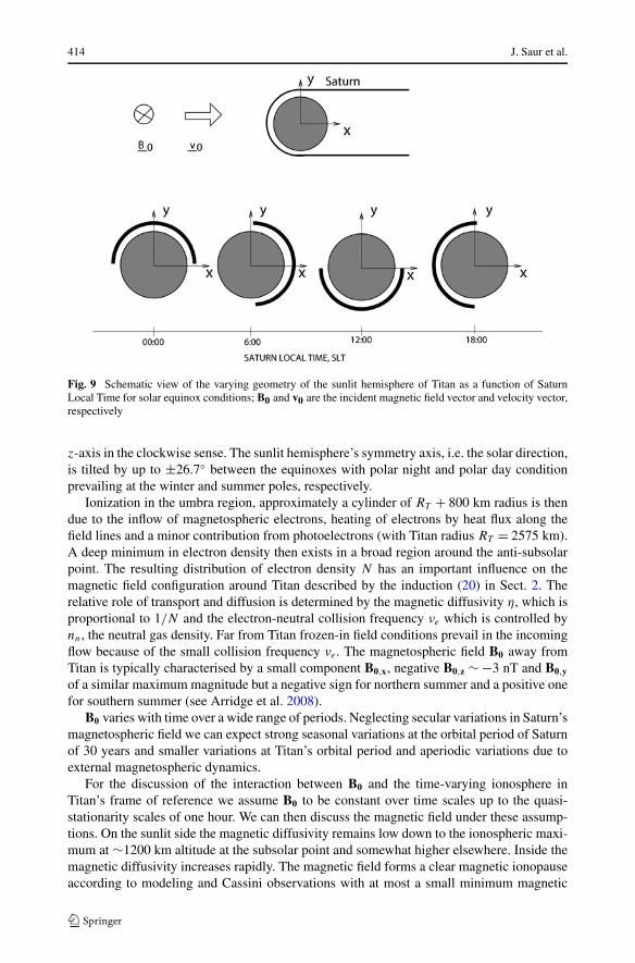
414 J. Saur et al.

Fig. 9 Schematic view of the varying geometry of the sunlit hemisphere of Titan as a function of SaturnLocal Time for solar equinox conditions; B0 and v0 are the incident magnetic field vector and velocity vector,respectively

z-axis in the clockwise sense. The sunlit hemisphere’s symmetry axis, i.e. the solar direction,is tilted by up to ±26.7◦ between the equinoxes with polar night and polar day conditionprevailing at the winter and summer poles, respectively.

Ionization in the umbra region, approximately a cylinder of RT + 800 km radius is thendue to the inflow of magnetospheric electrons, heating of electrons by heat flux along thefield lines and a minor contribution from photoelectrons (with Titan radius RT = 2575 km).A deep minimum in electron density then exists in a broad region around the anti-subsolarpoint. The resulting distribution of electron density N has an important influence on themagnetic field configuration around Titan described by the induction (20) in Sect. 2. Therelative role of transport and diffusion is determined by the magnetic diffusivity η, which isproportional to 1/N and the electron-neutral collision frequency νe which is controlled bynn, the neutral gas density. Far from Titan frozen-in field conditions prevail in the incomingflow because of the small collision frequency νe . The magnetospheric field B0 away fromTitan is typically characterised by a small component B0,x, negative B0,z ∼ −3 nT and B0,y

of a similar maximum magnitude but a negative sign for northern summer and a positive onefor southern summer (see Arridge et al. 2008).

B0 varies with time over a wide range of periods. Neglecting secular variations in Saturn’smagnetospheric field we can expect strong seasonal variations at the orbital period of Saturnof 30 years and smaller variations at Titan’s orbital period and aperiodic variations due toexternal magnetospheric dynamics.

For the discussion of the interaction between B0 and the time-varying ionosphere inTitan’s frame of reference we assume B0 to be constant over time scales up to the quasi-stationarity scales of one hour. We can then discuss the magnetic field under these assump-tions. On the sunlit side the magnetic diffusivity remains low down to the ionospheric maxi-mum at ∼1200 km altitude at the subsolar point and somewhat higher elsewhere. Inside themagnetic diffusivity increases rapidly. The magnetic field forms a clear magnetic ionopauseaccording to modeling and Cassini observations with at most a small minimum magnetic


field magnitude below the ionopause. Because of the much lower electron densities magneticdiffusion is much more important on the night side, i.e. in the umbra. The combined actionof magnetic diffusion and inflow of plasma leads to the strongest appearance of magneticfields below the ionosphere in the lower neutral atmosphere at less than 800 km altitude,say. When Titan is at SLT ∼6.00 h, we expect the maximum inducing field perpendicular tothe x-axis to occur close to or on the (−x)-axis, i.e. at the center of the ramside hemisphere.As Titan moves along its orbit during a Titan day for any given point fixed to Titan the in-ducing field is at most very small on the sunlit side, grows in the umbra, where it reaches amaximum near its center, to fall off towards the sunlit side again.

It is clear from the discussion including Fig. 9 that a constant incident B0 leads to aninducing field below the ionosphere, which at any position (x, y, z) can be described by aFourier series in time with the fundamental frequency ΩT derived from a Titan day. In re-ality B0 will not be constant in time but vary at many frequencies Ω . For a given frequencyΩ in B0 and ΩT describing the rotation of the solar energy source in Fig. 9 the interactionbetween the plasma flow and the magnetic field described by (20) and the full set of fluid(or kinetic) equations (not given in this manuscript) then leads to the inducing fields Bi(t)

below the ionosphere. At any given location Bi(t) must then be composed of a componentconstant in time, harmonic components at frequencies Ω and ΩT and multiples thereof andfrequencies abs(ΩT ± Ω) etc. due to the non-linearities in the interaction. There will becontributions to Ω due to the SLT-variation of the magnetosphere and more importantly dueto the synodic rotation period of Saturn TS,syn,T = 10.8 h as seen from Titan. Interestingly,there will not only be small variations in B0(t) but also in the rotating plasma properties atTS,syn,T enhancing the inducing signal at the relatively high corresponding frequency (Ar-ridge et al. 2008). This leads to lower conductivity requirements of about 2.2 S/m for theocean with some remaining weak dependence on mantle properties. All frequency peakswill be smeared by aperiodic dynamic variations. In the frame of Titan there will also be asmall component of the magnetic field that is constant in time and therefore penetrates Ti-tan completely. The induction investigation could be done using an array of magnetometerson the surface of Titan over several Titan days. A less demanding approach could use anorbiter with repeated measurements at the pericenter x ≈ −900 km and y ≈ 0, z ≈ 0 andother locations distributed around Titan with measurements over at least several Titan days.The data analysis will also require straightforward 3D-modeling along the lines of Schillinget al. (2007).

Finally, there is always the possibility of induction studies using spacecraft encountersoccurring under serendipitous conditions like strong Saturnian magnetospheric dynamics inresponse to the solar wind dynamics. In addition, observations near Titan at times when thesun is eclipsed by Saturn would be very useful around equinox conditions.

7 Uranus, Neptune and Beyond

Compared to the Saturn system, the Uranus and Neptune systems are paradises for inductionstudies. Uranus’ axial tilt, i.e. the angle between its spin axis and the normal to its orbitalplane, is 97.8◦. Uranus’ magnetic field can be represented to first order by a dipole momentof 2.3×104 nT (4π/μ0)R

3U , where RU = 25,600 km is Uranus’ planetary radius (Ness et al.

1986). The dipole is offset from the center of the planet by 0.3RU . It is also inclined withrespect to Uranus’ spin axis by 60◦. The rotation period of the magnetic field of 17.3 h isused to define Uranus’ rotation period (Ness et al. 1986). Uranus’ satellites Ariel, Umbriel,Titania and Oberon have diameters larger than 1000 km and small inclination and eccentric-ity. Up to now no magnetic field data are available near these satellites, but future spacecraft

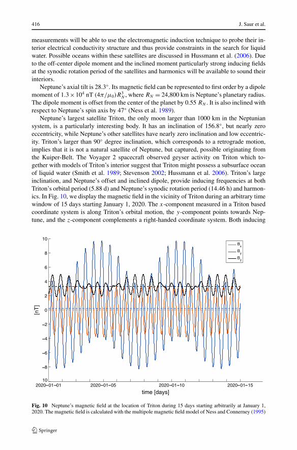
416 J. Saur et al.

measurements will be able to use the electromagnetic induction technique to probe their in-terior electrical conductivity structure and thus provide constraints in the search for liquidwater. Possible oceans within these satellites are discussed in Hussmann et al. (2006). Dueto the off-center dipole moment and the inclined moment particularly strong inducing fieldsat the synodic rotation period of the satellites and harmonics will be available to sound theirinteriors.

Neptune’s axial tilt is 28.3◦. Its magnetic field can be represented to first order by a dipolemoment of 1.3×104 nT (4π/μ0)R

3N , where RN = 24,800 km is Neptune’s planetary radius.

The dipole moment is offset from the center of the planet by 0.55 RN . It is also inclined withrespect to Neptune’s spin axis by 47◦ (Ness et al. 1989).

Neptune’s largest satellite Triton, the only moon larger than 1000 km in the Neptuniansystem, is a particularly interesting body. It has an inclination of 156.8◦, but nearly zeroeccentricity, while Neptune’s other satellites have nearly zero inclination and low eccentric-ity. Triton’s larger than 90◦ degree inclination, which corresponds to a retrograde motion,implies that it is not a natural satellite of Neptune, but captured, possible originating fromthe Kuiper-Belt. The Voyager 2 spacecraft observed geyser activity on Triton which to-gether with models of Triton’s interior suggest that Triton might possess a subsurface oceanof liquid water (Smith et al. 1989; Stevenson 2002; Hussmann et al. 2006). Triton’s largeinclination, and Neptune’s offset and inclined dipole, provide inducing frequencies at bothTriton’s orbital period (5.88 d) and Neptune’s synodic rotation period (14.46 h) and harmon-ics. In Fig. 10, we display the magnetic field in the vicinity of Triton during an arbitrary timewindow of 15 days starting January 1, 2020. The x-component measured in a Triton basedcoordinate system is along Triton’s orbital motion, the y-component points towards Nep-tune, and the z-component complements a right-handed coordinate system. Both inducing

Fig. 10 Neptune’s magnetic field at the location of Triton during 15 days starting arbitrarily at January 1,2020. The magnetic field is calculated with the multipole magnetic field model of Ness and Connerney (1995)


frequencies are clearly visible in Fig. 10. The time averaged fields are shown as dashed lines.The average Bz is ∼3 nT and often smaller in magnitude than the time variable components.The strong time variable components at both frequencies might resolve the thickness andthe conductivity of a possible ocean independently (see discussion in Sect. 5.2).

Possible subsurface oceans are also being discussed for large Kuiper-Belt objects suchas Pluto, Charon, Eris, Sedna (Stevenson 2002; Hussmann et al. 2006). These bodies areimmersed in the solar wind (based on the current state of knowledge). Therefore no imme-diately obvious time periodic field is available that can be used in future spacecraft flybys.Two spacecraft near these objects would allow for an observational setup where one de-termines the time-varying field while the other one, closer to the body, could measure theinductive response. Asteroids might be similarly sounded with the induction method.

Induction possibly also plays an important role for extra-solar planets. Planets very closeto the central star might be exposed to large time-varying stellar magnetic fields. Laineet al. (2008) discuss the possibility that Ohmic dissipation due to induction caused by shortperiod planets could be large enough to inflate the planet and significantly contribute to massloss. The Ohmic heating however does not provide a significant heat source in the possiblesubsurface ocean of the solar system satellites discussed in this chapter when compared totidal heating in the icy crust and the inner parts of the satellites (Hussmann et al. 2002;Tovie et al. 2005). For the solar system bodies, tidal dissipation of Rossby waves within thepossible ocean might also significantly contribute to the heating of the oceans (Tyler 2008).

Finally, the induction technique can also be applied to all six non-discussed planets ofour solar system, similar to how it is applied at Earth to probe the interior of the Earth (e.g.,Schmucker 1985; Olsen 1999; Constable and Constable 2004). This could be achieved byorbiting spacecraft at small radial distances from the planets.

Acknowledgements We thank Nico Schilling, Nils Olsen, Stefan Duling and Mario Seufert for valuablecontributions to this chapter. We appreciate helpful comments by the referee on the presentation of the man-uscript. JS acknowledges financial support by Deutsche Forschungsgesellschaft. The work by KHG wasfinancially supported by the German Ministerium für Wirtschaft und Technologie and the German Zentrumfür Luft- und Raumfahrt under contract 50 QW 0602.

References

M.H. Acuña, N.F. Ness, The magnetic field of Saturn–Pioneer 11 observations. Science 207, 444–446 (1980)B.J. Anderson, M.H. Acuña, D.A. Lohr, J. Scheifele, A. Raval, H. Korth, J.A. Slavin, The magnetometer

instrument on MESSENGER. Space Sci. Rev. 131, 417–450 (2007). doi:10.1007/s11214-007-9246-7B.J. Anderson, M.H. Acuña, H. Korth, M.E. Purucker, C.L. Johnson, J.A. Slavin, S.C. Solomon, R.L. McNutt,

The structure of Mercury’s magnetic field from MESSENGER’s first flyby. Science 321, 82 (2008).doi:10.1126/science.1159081

J.D. Anderson, G. Schubert, R.A. Jacobson, E.L. Lau, W.B. Moore, W.L. Sjogren, Europa’s differentiatedinternal structure: Inferences from four Galileo encounters. Science 281, 2019–2022 (1998)

C. Arridge, N. Andre, N. Achilleos, et al., Thermal electron periodicities at 20rs in Saturn’s magnetosphere.Geophys. Res. Lett. 35, 15 (2008)

H. Backes, et al., Titan’s magnetic field signature during the first Cassini encounter. Science 308, 992–995(2005)

W. Baumjohann, R.A. Treumann, Basic Space Plasma Physics (Imperial College Press, London, 1996)J.L. Blank, W.R. Sill, Response of the Moon to the time-varying interplanetary magnetic field. J. Geophys.

Res. 74, 736–743 (1969). doi:10.1029/JA074i003p00736J.E.P. Connerney, M.H. Acuna, N.F. Ness, T. Satoh, New models of Jupiter’s magnetic field constrained by

the Io Flux Tube footprint. J. Geophys. Res. 103, 11929–11939 (1998)S. Constable, C. Constable, Observing geomagnetic induction in magnetic satellite measurements and as-

sociated implications for mantle conductivity. Geochem. Geophys. Geosyst. 5 (2004). doi:10.1029/2003GC000634

http://dx.doi.org/10.1007/s11214-007-9246-7

http://dx.doi.org/10.1126/science.1159081

http://dx.doi.org/10.1029/JA074i003p00736

http://dx.doi.org/10.1029/2003GC000634

http://dx.doi.org/10.1029/2003GC000634

418 J. Saur et al.

T.E. Cravens, et al., Titan’s ionosphere: Model comparisons with Cassini Ta data. Geophys. Res. Lett. 32,12108 (2005)

M.K. Dougherty, N. Achilleos, N. Andre, C.S.A.A. Balogh, C. Bertucci, et al., Cassini magnetometer obser-vations during Saturn orbit insertion. Science 307, 1266–1270 (2005)

M.K. Dougherty, K.K. Khurana, F.M. Neubauer, C.T. Russell, J. Saur, J.S. Leisner, M. Burton, Identificationof a dynamic atmosphere at Enceladus with the Cassini Magnetometer. Science 311, 1406 (2006)

P. Dyal, D.I. Gordon, Lunar surface magnetometers. IEEE Trans. Magn. 9, 226–231 (1973). doi:10.1109/TMAG.1973.1067650

P. Dyal, C.W. Parkin, Global electromagnetic induction in the Moon and planets. Phys. Earth Planet. Inter. 7,251–265 (1973). doi:10.1016/0031-9201(73)90052-6

P. Dyal, C.W. Parkin, D. W.D., Magnetism and the interior of the moon. Rev. Geophys. Space Phys. 12,568–591 (1975)

S. Espinosa, M. Dougherty, Periodic perturbations in Saturn’s magnetic field. Geophys. Res. Lett. 27, 2785–2788 (2000)

S. Espinosa, D. Southwood, M. Dougherty, How can Saturn impose its rotation period in a noncorotatingmagnetosphere? J. Geophys. Res. 108, 11–1 (2003)

L.W. Esposito, J.E. Colwell, K. Larsen, et al., Ultraviolet imaging spectroscopy shows an active Saturniansystem. Science 307, 1251 (2005)

F.P. Fanale, Y.P. Li, E. Decarlo, C. Farley, S. Sharma, K. Horton, An experimental estimate of Europa’s“ocean” composition independent of Galileo orbital remote sensing. J. Geophys. Res. 106, 14595–14600(2001)

G. Giampieri, M. Dougherty, C.T. Smith, E.J. Russell, A regular period for Saturn’s magnetic field that maytrack its internal rotation. Nature 441, 62–64 (2006)

K.H. Glassmeier, H.U. Auster, U. Motschmann, A feedback dynamo generating Mercury’s magnetic field.Geophys. Res. Lett. 34, 22201–22205 (2007a). doi:10.1029/2007GL031662

K.H. Glassmeier, J. Grosser, U. Auster, D. Constantinescu, Y. Narita, S. Stellmach, Electromagnetic in-duction effects and dynamo action in the Hermean system. Space Sci. Rev. 132, 511–527 (2007b).doi:10.1007/s11214-007-9244-9

K.H. Glassmeier, H. Auster, D. Heyner, K. Okrafka, C. Carr, G. Berghofer, B.J. Anderson, A. Balogh,W. Baumjohann, P.J. Cargill, U. Christensen, M. Delva, M. Dougherty, K. Fornaçon, T.S. Horbury,E.A. Lucek, W. Magnes, M. Mandea, A. Matsuoka, M. Matsushima, U. Motschmann, R. Nakamura,Y. Narita, I. Richter, K. Schwingenschuh, H. Shibuya, J.A. Slavin, C. Sotin, B. Stoll, H. Tsunakawa,S. Vennerstrom, J. Vogt, T. Zhang, The fluxgate magnetometer of the BepiColombo planetary orbiter.Planet. Space Sci. (2009)

O. Grasset, C. Sotin, F. Deschamps, On the internal structure and dynamics of titan. Planet. Space Sci. 48,617–636 (2000)

P.M. Grindrod, A.D. Fortes, F. Nimmo, et al., The long-term stability of a possible aqueous ammonium sulfateocean inside titan. Icarus 197, 137–151 (2008)

J. Grosser, K.H. Glassmeier, A. Stadelmann, Induced magnetic field effects at planet Mercury. Planet. SpaceSci. 52, 1251–1260 (2004). doi:10.1016/j.pss.2004.08.005

D.A. Gurnett, W.S. Kurth, A. Roux, S.J. Bolton, C.F. Kennel, Galileo plasma wave observations in the Ioplasma torus and near Io. Science 274, 391–392 (1996)

D.A. Gurnett, et al., The variable rotation period of the inner region of Saturn’s plasma disk. Science 316,442–445 (2007)

D.T. Hall, D.F. Strobel, P.D. Feldman, M.A. McGrath, H.A. Weaver, Detection of an oxygen atmosphere onJupiter’s moon Europa. Nature 373(6516), 677–679 (1995)

K.P. Hand, C.F. Chyba, Empirical constraints on the salinity of the European ocean and implications for athin ice shell. Icarus 189, 424–438 (2007)

C.J. Hansen, et al., Enceladus’ water vapor plume. Science 311, 1422–1425 (2006)D. Heyner, D. Schmitt, J. Wicht, K.H. Glassmeier, H. Korth, U. Motschmann, Concerning the initial temporal

evolution of a Hermean feedback dynamo. Earth Planet. Sci. Lett. (2009)B.A. Hobbs, L.L. Hood, F. Herbert, C.P. Sonett, An upper bound on the radius of a highly electrically con-

ducting lunar core. J. Geophys. Res. 88, 97 (1983). doi:10.1029/JB088iS01p00B97L. Hood, G. Schubert, Inhibition of solar wind impingement on Mercury by planetary induction currents.

J. Geophys. Res. 84, 2641–2647 (1979)L.L. Hood, F. Herbert, C.P. Sonett, The deep lunar electrical conductivity profile—Structural and thermal

inferences. J. Geophys. Res. 87, 5311–5326 (1982). doi:10.1029/JB087iB07p05311R. Hunten, et al., Saturn (Univ. of Arizona Press, Tucson, 1984)T. Hurford, P. Helfenstein, G. Hoppa, R. Greenberg, B. Bills, Eruptions arising from tidally controlled peri-

odic openings of rifts on Enceladus. Nature 447, 292–294 (2007)

http://dx.doi.org/10.1109/TMAG.1973.1067650

http://dx.doi.org/10.1109/TMAG.1973.1067650

http://dx.doi.org/10.1016/0031-9201(73)90052-6

http://dx.doi.org/10.1029/2007GL031662

http://dx.doi.org/10.1007/s11214-007-9244-9

http://dx.doi.org/10.1016/j.pss.2004.08.005

http://dx.doi.org/10.1029/JB088iS01p00B97

http://dx.doi.org/10.1029/JB087iB07p05311


H. Hussmann, T. Spohn, K. Wieczerkowski, Thermal equilibrium states of Europa’s ice shell: Implicationsfor internal ocean thickness and surface heat flow. Icarus 156, 143–151 (2002)

H. Hussmann, F. Sohl, T. Spohn, Subsurface oceans and deep interiors of medium-sized outer planet satellitesand large trans-Neptunian objects. Icarus 185, 258–273 (2006)

X. Jia, R. Walker, M. Kivelson, K. Khurana, J. Linker, Three-dimensional MHD simulations of Ganymede’smagnetosphere. J. Geophys. Res. 113, 06212 (2008)

J. Kargel, J. Kaye, J. Head, G. Marion, R. Sassen, O.P. Ballesteros, S. Grant, D. Hogenboom, Europa’s crustand ocean: Origin, composition and the prospects for life. Icarus 148, 368–390 (2000)

C. Keller, T.E. Cravens, L. Gan, One-dimensional multispecies hydrodynamic models of the ramsideionosphere of titan. J. Geophys. Res. 99, 6511–6525 (1994)

A. Khan, J.A.D. Connolly, N. Olsen, K. Mosegaard, Constraining the composition and thermal state of themoon from an inversion of electromagnetic lunar day-side transfer functions. Earth Planet. Sci. Lett.248, 579–598 (2006). doi:10.1016/j.epsl.2006.04.008

K.K. Khurana, M.G. Kivelson, D.J. Stevenson, G. Schubert, C.T. Russell, R.J. Walker, C. Polanskey, Inducedmagnetic fields as evidence for subsurface oceans in Europa and Callisto. Nature 395, 777–780 (1998)

K.K. Khurana, M.G. Kivelson, C.T. Russell, Searching for liquid water in Europa by using surface observa-tions. Astrobiol. J. 2, 93–103 (2002)

K.K. Khurana, et al., The configuration of Jupiter’s magnetosphere, in Jupiter, ed. by F. Bagenal (Cam-bridge Univ. Press, Cambridge, 2004), pp. 593–616, Chap. 24

M.G. Kivelson, K.K. Khurana, R.J. Walker, C.T. Russell, J.A. Linker, D.J. Southwood, C. Polanskey, A mag-netic signature at Io: Initial report from the Galileo magnetometer. Science 273, 337–340 (1996)

M.G. Kivelson, K.K. Khurana, S. Joy, C.T. Russell, D.J. Southwood, R.J. Walker, C. Polanskey, Europa’smagnetic signature: Report from Galileo’s first pass on 19 December 1996. Science 276, 1239–1241(1997)

M.G. Kivelson, K.K. Khurana, D.J. Stevenson, L. Bennett, S. Joy, C.T. Russell, R.J. Walker, C. Zimmer,C. Polanskey, Europa and Callisto: Induced or intrinsic fields in a periodically varying plasma environ-ment. J. Geophys. Res. 104(A3), 4609–4625 (1999)

M.G. Kivelson, K.K. Khurana, C.T. Russell, M. Volwerk, J. Walker, C. Zimmer, Galileo magnetometer mea-surements: A stronger case for a subsurface ocean at Europa. Science 289(5483), 1340–1343 (2000)

M.G. Kivelson, K.K. Khurana, M. Volwerk, The permanent and inductive magnetic moments of Ganymede.Icarus 157, 507–522 (2002)

M.G. Kivelson, F. Bagenal, F.M. Neubauer, W. Kurth, C. Paranicas, J. Saur, Magnetospheric interactionswith satellites, in Jupiter, ed. by F. Bagenal (Cambridge Univ. Press, Cambridge, 2004), pp. 513–536,Chap. 21

A.J. Kliore, D.P. Hinson, F.M. Flasar, A.F. Nagy, T.E. Cravens, The ionosphere of Europa from Galileo radiooccultations. Science 277(5324), 355–358 (1997)

A. Kopp, W. Ip, Resistive MHD simulations of Ganymede’s magnetosphere 1. Time variabilities of the mag-netic field topology. J. Geophys. Res. 107, 41–11490 (2002)

B.N. Lahiri, A.T. Price, Electromagnetic induction in non-uniform conductors. Philos. Trans. R. 784(A 237),509–540 (1939)

R. Laine, D. Lin, S. Dong, Interaction of close-in planets with the magnetosphere of their host stars. 1.Diffusion, Ohmic dissipation of time-dependent field, planetary inflation, and mass loss. Astrophys. J.685, 521–542 (2008)

R.D. Lorenz, B.W. Stiles, R.L. Kirk, et al., Titan’s rotation reveals an internal ocean and changing zonalwinds. Science 319, 1649 (2008)

Y. Ma, et al., Comparisons between MHD model calculations and observations of Cassini flybys of Titan.J. Geophys. Res. 111, 05207 (2006)

W. McKinnon, M. Zolensky, Sulfate content of Europa’s ocean and shell: Evolutionary considerations andsome geological and strobiological implications. Astrobiology 3, 879–897 (2003)

N.F. Ness, J.E.P. Connerney, Neptune’s magnetic field and field-geometric properties, in Neptune and Triton,ed. by D.P. Cruikshank (Univ. of Arizona Press, Tucson, 1995), pp. 141–168

N.F. Ness, K.W. Behannon, R.P. Lepping, Y.C. Whang, K.H. Schatten, Magnetic field observations nearMercury: preliminary results from Mariner 10. Science 185, 131–135 (1974)

N.F. Ness, M.H. Acuña, K.W. Behannon, L.F. Burlaga, J. Connerney, R.P. Lepping, F.M. Neubauer, Magneticfields at Uranus. Science 233, 85–89 (1986)

N.F. Ness, M.H. Acuña, L.F. Burlaga, J. Connerney, R.P. Lepping, F.M. Neubauer, Magnetic fields at Nep-tune. Science 246, 1473–1478 (1989)

F.M. Neubauer, Nonlinear standing Alfvén wave current system at Io: Theory. J. Geophys. Res. 85(A3),1171–1178 (1980)

F.M. Neubauer, The sub-Alfvénic interaction of the Galilean satellites with the Jovian magnetosphere. J. Geo-phys. Res. 103(E9), 19843–19866 (1998)

http://dx.doi.org/10.1016/j.epsl.2006.04.008

420 J. Saur et al.

F.M. Neubauer, Alfvén wings and electromagnetic induction in the interiors: Europa and Callisto. J. Geo-phys. Res. 104(A12), 28671 (1999)

N. Olsen, Induction studies with satellite data. Surv. Geophys. 20, 309–340 (1999)N. Olsen, et al., Separation of magnetic field into external and internal parts, in Planetary Magnetism

(Springer, Berlin, 2009)R.T. Pappalardo, et al., Does Europa have a subsurface ocean? Evaluation of the geological evidence. J. Geo-

phys. Res. 104, 24015–24056 (1999)W. Parkinson, Introduction of Geomagnetism (Scottish Academic Press, Edinburgh, 1983)C. Paty, R. Winglee, Multi-fluid simulations of Ganymede’s magnetosphere. Geophys. Res. Lett. 31, 24806

(2004)C. Porco, et al., Cassini observes the active south pole of Enceladus. Science 311, 1393–1401 (2006)F. Postberg, S. Kempf, J. Schmidt, N. Brillantov, A. Beinsen, B. Abel, U. Buck, R. Srama, Sodium salts in

E-ring ice grains from an ocean below the surface of Enceladus. Nature 459, 1098–1101 (2009)T. Rikitake, Electromagnetism and the Earth’s Interior (Elsevier, Amsterdam, 1966)J. Saur, A model for Io’s local electric field for a combined Alfvénic and unipolar inductor far-field coupling.

J. Geophys. Res. 109, 01210 (2004)J. Saur, D.F. Strobel, F.M. Neubauer, Interaction of the Jovian magnetosphere with Europa: Constraints on

the neutral atmosphere. J. Geophys. Res. 103(E9), 19947–19962 (1998)J. Saur, F.M. Neubauer, D.F. Strobel, M.E. Summers, Interpretation of Galileo’s Io plasma and field ob-

servations: The J0, I24, I27 flybys, and close polar passes. J. Geophys. Res. 107(A12), 1422 (2002).doi:10.1029/2001JA005067

J. Saur, F.M. Neubauer, N. Schilling, Hemisphere coupling in Enceladus’ asymmetric plasma interaction.J. Geophys. Res. 112, 11209 (2007). doi:10.1029/2007JA012479

J. Saur, N. Schilling, F.M. Neubauer, et al., Evidence for temporal variability of Enceladus’ gas jets: Modelingof Cassini observations. Geophys. Res. Lett. 35, 20105 (2008)

N. Schilling, K.K. Khurana, M.G. Kivelson, Limits on an intrinsic dipole moment in Europa. J. Geophys. Res.109, 05006 (2004)

N. Schilling, F.M. Neubauer, J. Saur, Time-varying interaction of Europa with the Jovian magnetosphere:Constraints on the conductivity of Europa’s subsurface ocean. Icarus 192, 41–55 (2007)

N. Schilling, F.M. Neubauer, J. Saur, Influence of the internally induced magnetic field on the plasma inter-action of Europa. J. Geophys. Res. 113, 03203 (2008)

J. Schmidt, N. Brilliantov, F. Spahn, S. Kempf, Slow dust in Enceladus’ plume from condensation and wallcollisions in tiger stripe fractures. Science 451, 685–688 (2008)

U. Schmucker, Magnetic and electric fields due to electromagnetic induction by external sources, in Landolt-Börnstein New-Series, 5/2b (Springer, Berlin–Heidelberg, 1985), pp. 100–125

G. Schubert, J. Anderson, B. Travis, J. Palguta, Enceladus: Present internal structure and differentiation byearly and long-term radiogenic heating. Icarus 188, 345–355 (2007)

M. Siegert, J. Ellis-Evans, M. Tranter, C. Mayer, J.R. Petit, A. Salamatin, J. Priscu, Physical, chemical andbiological processes in Lake Vostok and other Antarctic subglacial lakes. Nature 416, 603–609 (2001)

M. Siegert, S. Carter, I. Tabacco, S. Popov, D. Blankenship, A revised inventory of Antarctic subglacial lakes.Antarct. Sci. 17, 453–460 (2005)

S. Simon, A. Bößwetter, T. Bagdonat, U. Motschmann, K.H. Glassmeier, Plasma environment of Titan: a 3-Dhybrid simulation study. Ann. Geophys. 24, 1113–1135 (2006)

G. Siscoe, L. Christopher, Variations in the solar wind stand-off distance at Mercury. Geophys. Res. Lett. 2,158–160 (1975)

B.A. Smith, L. Soderblom, R. Batson, P. Bridges, J. Inge, H. Masursky, A new look at the Saturn system: Thevoyager 2 images. Science 215, 505–537 (1982)

B.A. Smith, et al., Voyager 2 at Neptune: imaging science results. Science 246, 1422–1449 (1989)E. Smith, L. Davis, D. Jones, P. Coleman, D. Colburn, P. Dyal, C. Sonett, Saturn’s magnetic field and mag-

netosphere. Science 207, 407–410 (1980)B. Smith-Konter, R.T. Pappalardo, Tidally driven stress accumulation and shear failure of Enceladus’ tiger

stripes. Icarus 198, 435 (2008)F. Sohl, H. Hussmann, B. Schwentker, T. Spohn, R.D. Lorenz, Interior structure models and tidal love num-

bers of titan. J. Geophys. Res. 108, 4–1 (2003)C.P. Sonett, Electromagnetic induction in the moon. Rev. Geophys. Space Phys. 20, 411–455 (1982)C.P. Sonett, P. Dyal, C.W. Parkin, D.S. Colburn, J.D. Mihalov, B.F. Smith, Whole body response of the moon

to electromagnetic induction by the solar wind. Science 172, 256–258 (1971)D.J. Southwood, M.G. Kivelson, Saturnian magnetospheric dynamics: Elucidation of a camshaft model.

J. Geophys. Res. 112, 12 (2007)F. Spahn, et al., Cassini dust measurements at Enceladus and implications for the origin of the E-ring. Science

311, 1416–1418 (2006)

http://dx.doi.org/10.1029/2001JA005067

http://dx.doi.org/10.1029/2007JA012479


B.J. Srivastava, Theory of the magnetotelluric method of a spherical conductor. Geophys. J. R. Astron. Soc.11, 373–387 (1966)

D. Stevenson, Planetary oceans. Sky Telesc. 104, 38–44 (2002)D.J. Stevenson, Planetary magnetic fields. Earth Planet. Sci. Lett. 208, 1–2 (2003). doi:10.1016/S0012-

821X(02)01126-3S.T. Suess, B.E. Goldstein, Compression of the Hermean magnetosphere by the solar wind. J. Geophys. Res.

84, 3306–3312 (1979)W.M. Telford, Applied Geophysics (Cambridge University Press, Cambridge, 1993)R. Tokar, et al., The interaction of the atmosphere of Enceladus with Saturn’s plasma. Science 311, 1409–

1412 (2006)G. Tovie, A. Mocquet, C. Sotin, Tidal dissipation within large icy satellites: Applications to Europa and Titan.

Icarus 177, 534–549 (2005)R.H. Tyler, S. Maus, H. Lühr, Satellite observations of magnetic fields due to ocean tidal flow. Science 239,

239–241 (2003)R.H. Tyler, Strong ocean tidal flow and heating on moons of the outer planets. Nature 456, 770–772 (2008)L.L. Vanyan, I.V. Egorov, Electromagnetic induction in the moon. Moon 12, 253–275 (1975). doi:10.1007/

BF02629697G.H. Voigt, A mathematical magnetospheric field model with independent physical parameters. Planet. Space

Sci. 29, 1–20 (1981). doi:10.1016/0032-0633(81)90134-3J. Waite, et al., Cassini ion and neutral mass spectrometer: Enceladus plume composition and structure.

Science 311, 1419–1409 (2006)J. Wicht, M. Mandea, F. Takahashi, U.R. Christensen, M. Matsushima, B. Langlais, The origin of Mercury’s

internal magnetic field. Space Sci. Rev. 132, 261–290 (2007). doi:10.1007/s11214-007-9280-5C. Zimmer, K. Khurana, M. Kivelson, Subsurface oceans on Europa and Callisto: Constraints from Galileo

magnetometer observations. Icarus 147, 329–347 (2000)M.Y. Zolotov, An oceanic composition on early and today’s Enceladus. Geophys. Res. Lett. 34, 23 (2007)M.Y. Zolotov, E. Shock, Composition and stability of salts on the surface of Europa and their oceanic origin.

J. Geophys. Res. 106, 32815–32827 (2001)

http://dx.doi.org/10.1016/S0012-821X(02)01126-3

http://dx.doi.org/10.1016/S0012-821X(02)01126-3

http://dx.doi.org/10.1007/BF02629697

http://dx.doi.org/10.1007/BF02629697

http://dx.doi.org/10.1016/0032-0633(81)90134-3

http://dx.doi.org/10.1007/s11214-007-9280-5

Induced Magnetic Fields in Solar System Bodies · Induced Magnetic Fields in Solar System Bodies...

Documents

Transcript of Induced Magnetic Fields in Solar System Bodies · Induced Magnetic Fields in Solar System Bodies...