The Astrophysical Journal, 722:577–585, 2010 October 10 doi:10.1088/0004-637X/722/1/577C© 2010. The American Astronomical Society. All rights reserved. Printed in the U.S.A.

QUANTIFYING THE EVOLVING MAGNETIC STRUCTURE OF ACTIVE REGIONS

Paul A. Conlon1, R.T. James McAteer

1,2, Peter T. Gallagher

1, and Linda Fennell

11 School of Physics, Trinity College Dublin, Dublin 2, Ireland

2 Department of Astronomy, New Mexico State University, NM 88003-8001, USA; mcateer@nmsu.eduReceived 2010 April 26; accepted 2010 August 3; published 2010 September 22

ABSTRACT

The topical and controversial issue of parameterizing the magnetic structure of solar active regions has vitalimplications in the understanding of how these structures form, evolve, produce solar flares, and decay. Thisinterdisciplinary and ill-constrained problem of quantifying complexity is addressed by using a two-dimensionalwavelet transform modulus maxima (WTMM) method to study the multifractal properties of active regionphotospheric magnetic fields. The WTMM method provides an adaptive space-scale partition of a fractal distribution,from which one can extract the multifractal spectra. The use of a novel segmentation procedure allows us to removethe quiet Sun component and reliably study the evolution of active region multifractal parameters. It is shownthat prior to the onset of solar flares, the magnetic field undergoes restructuring as Dirac-like features (with aHolder exponent, h = −1) coalesce to form step functions (where h = 0). The resulting configuration has ahigher concentration of gradients along neutral line features. We propose that when sufficient flux is presentin an active region for a period of time, it must be structured with a fractal dimension greater than 1.2, anda Holder exponent greater than −0.7, in order to produce M- and X-class flares. This result has immediateapplications in the study of the underlying physics of active region evolution and space weather forecasting.

Key words: magnetic fields – methods: statistical – Sun: flares – turbulence

1. INTRODUCTION

Solar active regions are concentrations of intense magneticfield in the atmosphere of the Sun. These highly dynamic,complex structures are rooted in the photosphere, extend intothe corona, and are the source of many extreme solar events,such as solar flares and coronal mass ejections (Gallagher et al.2007). Direct spatially localized measurements of the coronalmagnetic field are beyond current instrumentation, due to thetenuous nature of the Sun’s atmosphere. However, by studyingthe evolution of magnetic elements on the photosphere we cangain insight into the physical process that governs the formationand evolution of active regions in the corona.

The building blocks of active regions are flux tubes, whichare thought to be formed near the tachocline of the Sun (Miesch2005). Turbulent sub-surface forces result in a buoyant upwardmotion that cause the formation of Ω-like loops, which in turnemerge through the photosphere to form active regions. In thelow β corona, the plasma is restrained to flow along thesefield lines, thereby creating the loop-like structures evident inextreme ultraviolet images of the Sun. Sunspots are the visiblefootpoints of these active region loops and appear as collectionsof positive and negative polarity magnetic flux elements inmagnetograms. Flux constantly emerges through the surface ofthe Sun and interacts with existing active region flux. The systemis characterized by a large magnetic Reynolds number, given byRm = LV/η, where L, V, and η are the length scale, velocity,and the magnetic diffusivity on the photosphere; for typicalphotospheric values of these parameters the magnetic Reynoldsis ∼106–1010 (McAteer et al. 2010). Hence, the photosphere isconsidered a highly turbulent and chaotic environment.

Further evidence of the turbulent nature of active regionsis found in the distribution of magnetic flux on the surfaceof the Sun (Vlahos 2002; Abramenko 2005b; Hewett et al.2008). The distribution of magnetic flux within active regionsfollows a power-law distribution, suggesting a self-organized

structure and hence numerous nonlinear techniques have beenused to study the evolution of active regions (Abramenko 2005a;Abramenko et al. 2008; McAteer et al. 2005a; Conlon et al.2008; Aschwanden & Aschwanden 2008). One common methodof examining the self similar distribution of active region fluxis the fractal dimension. McAteer et al. (2005a) examined 104

active region images, related solar flares within a 24 hr window,and found that a fractal dimension of 1.2–1.25 was a minimumrequirement for an active region to produce solar flares. Conlonet al. (2008) similarly used a modified box-counting techniqueto examine the multifractal properties of evolving active regions.They found that as a region developed toward a state favorableto producing solar flares, there was a decrease in both thebreadth and height of the multifractal spectrum. An additionalmethod used to examine the fractal and multifractal propertiesof active regions is the structure function (Abramenko 2005a;Abramenko et al. 2008). A structure function is defined as astatistical moment of the increments of a field and measures itsassociated intermittences. Abramenko et al. (2008) showed thatthere is a relation between systematic changes in the ratio ofcertain powers of the structure function at both the photosphericand chromospheric level. Georgoulis (2005, 2008) examined theproblems of event prediction with such methods, but supportedthe use of these methods as analytical tools for the understandingof the fundamental processes involved in the formation andevolution of active regions.

These methods face several problems in dealing with thedata presently available; they are threshold-dependent (i.e.,results depend on the value chosen to remove the surroundingquiet Sun component) and numerical errors combined withpoor spatial resolution result in large errors for large andnegative moments (Georgoulis 2005; Conlon et al. 2008). Themore stable and reliable wavelet transform modulus maxima(WTMM; Kestener et al. 2010) method is used in this paperin order to overcome these problems, and examine the fractalproperties of solar magnetogram data. The WTMM method

577

578 CONLON ET AL. Vol. 722

replaces the boxes from the traditional box-counting methodwith wavelets, which act as fuzzy boxes and are defined forboth finite and discrete domains. The observations are describedin Section 2. In Section 3, a short description of the WTMMand segmentation method is presented. Analysis of the fractalproperties of evolving active regions using this method is shownin Section 4. Our conclusion and future directions are then givenin Section 5.

2. OBSERVATIONS

The Michelson Doppler Imager (MDI; Scherrer et al. 1995)on board the Solar and Heliospheric Observatory (SOHO;Domingo et al. 1995) images the Sun on a 1024 × 1024 pixelCCD camera through a series of increasingly narrow filters.The final elements, a pair of tunable Michelson interferometers,enable MDI to record measurements of the line-of-sight pho-tospheric field with an FWHM bandwidth of 94 mÅ. In thispaper, 96 minute cadence magnetograms of the full disc areused, which have a pixel size of ∼2′′.

A series of magnetograms are analyzed to examine thedifferences in fractal properties between flaring and non-flaringactive regions. Six active regions were analyzed as they evolvedand rotated across the solar disk (NOAA AR 10488, 9878,10763, 10942, 10954, and 10956). Given the powerful nature ofthe WTMM method, and improved accuracy of the segmentationmethod (see Section 3.2), thresholding was not performed on thedata. The analysis of each data set was restricted to periods whenthe center of each active region was within ±60◦ of disk center,in order to decrease the errors associated with projection effects.Magnetograms were corrected assuming a radial field at eachpoint on the solar disk and assuming an equal-area cylindricalprojection method (Bugayevskiy & Snyder 1995; McAteer et al.2005b) when calculating the basic physical parameters of areaand flux.

3. METHOD

Traditional box-counting methods (Vlahos 2002) calculatethe multifractal parameters of active regions based on thedistribution of magnetic flux elements within magnetograms.These methods are prone to errors in the calculation of themultifractal parameters due to image thresholding, resolution,and instrument noise. Wavelet-based methods have been shownto be versatile tools for the study of active region magneticfeatures (Hewett et al. 2008; Ireland et al. 2008). The WTMMmethod is particularly versatile and has been used to study X-rayflare emission (McAteer et al. 2007) and aid in the automaticdetection of coronal loops (McAteer et al. 2010).

The WTMM method calculates the multifractal parametersbased on the distribution of gradients within each image acrossscale. As such, the multifractal parameters as calculated by theWTMM method are more robust to changes in the resolutionand signal-to-noise ratio of magnetogram images. Additionally,the removal of quiet Sun features can be naturally carried out ingradient space as opposed to pixel space, thereby removing theproblem of creating singular features in magnetogram imagesthat arises from normal thresholding. This segmentation of quietSun, along with the limited resolution of MDI magnetograms,does result in a reduced number of gradients upon whichregression can be performed. We used a moving average offive magnetogram images in order to overcome this issue. Inthis section, the main advantages of using the wavelet transformfor performing a multifractal analysis are reviewed.

3.1. Basics of the 2D Wavelet Tranform Modulus Maxima(WTMM) Method

A rigorous and complete mathematical description of theWTMM is available in Arneodo et al. (2000) and Kestener et al.(2010). Here, we provide a brief outline to assist the reader inunderstanding the technique, while retaining the terminologyof Arneodo et al. (2000). The three main parts of the WTMMare (1) carry out a wavelet transform, (2) extract the skeletonof lines of modulus maxima, and (3) compute the companionpartition functions.

It can be shown that a two-dimensional (2D) continuouswavelet transform, T, of any 2D image, f(x, y), at each location,b, can be obtained as the gradient vector of the image smoothedto various scales, a, by a dilating filter, φ,

Tψ [f ](b, a) = ∇{Tφ[f ](b, a)}= ∇{φb,a ∗ f }, (1)

where ψ is the gradient of the filter. For our work, this amountsto smoothing the data by a Gaussian and carrying out a gradientfilter in the two image axis, (x, y), to obtain T. The image is thensmoothed by a larger Gaussian and the operation is repeated.

At each scale, the WTMM edges are extracted at loca-tions where the wavelet transform modulus Mψ [f ](b, a) =|Tψ [f ](b, a)| is locally maximum in the direction ofTψ [f ](b, a). These WTMM points lie in connected maximachains. The wavelet transform skeleton is the set of maximalines Lx0 defined as the location where the modulus is a localmaximum along a maxima chain. These lines contain all theinformation about the local Holder regularity (h) properties ofthe image. Along a maxima line Lx0 that points to x0 in the limita → 0+, the wavelet transform modulus behaves as a power lawwith exponent h(x0),

Mψ [f ][Lx0 (a)] ∼ ah(x0). (2)

The partition function, Z , is calculated from the skeleton byrising the modulus maxima values to some moment, q (where qcan take any real value), and summing over all lines,

Z(q, a) =∑

L∈L(a)

Mψ [f ](x ∈ L, a)q, (3)

from which the scaling exponents, τ (q), are defined in the limitof small scales Z(q, a) ∼ aτ (q), a → 0+. However, ratherthan calculating τ (q), and carrying out a Legendre transformto obtain the multifractal spectrum, Arneodo et al. (2000)suggest computing the companion partition functions directly.The Boltzmann weighting of each skeletal line is defined asWψ [f ](q,L, a) = (Mψ [f ])q/Z(q, a), the two components ofthe multifractal spectra, D(h) are

h(q, a) =∑

L∈L(a)

ln |Mψ [f ](x, a)| Wψ [f ](q,L, a)

∼ ah(q), (4)

D(q, a) =∑

L∈L(a)

Wψ [f ](q,L, a) ln(Wψ [f ](q,L, a))

∼ aD(q), (5)

and the linear regime of Equations (4) and (5) are adapted toreflect the physical size of the feature under study.

No. 1, 2010 QUANTIFYING THE EVOLVING MAGNETIC STRUCTURE OF ACTIVE REGIONS 579

Figure 1. Top: wavelet transform gradients of NOAA 10488 at scales 7, 28, and 56 pixels. Middle: same as top after the segmentation method proposed by Kesteneret al. (2010). Bottom: same as top after the segmentation method used in present study (intercept of 40).

3.2. Segmentation Using the WTMM Method

The analysis of active region magnetic fields can be misinter-preted due to the contribution of statistical information from thesurrounding quiet Sun. It is important to minimize this contri-bution as much as possible, as the multifractal properties of thequiet Sun are statistically different from that of an active region(Kestener et al. 2010). One method of doing this is the reductionof the image size and therefore minimizing the contribution ofquiet Sun in the resulting analysis. However, the dynamic na-ture of active regions means an adaptive image size is requiredfor larger regions. Kestener et al. (2010) developed a more ad-vanced method for the segmentation of active and quiet Sunfeatures based on thresholds in the wavelet transform modulusspace. They propose to discard those skeletal lines which lie in aregion of M−a space (Equation (2)) to allow for the separationof active region and quiet Sun. Figure 1, second panel, illustratesthe effect of this segmentation and unfortunately the thresholdsremove weaker parts of the active region gradients along withthe quiet Sun features. As the goal of our work is the detectionof characteristic changes in the structure and complexity of anactive region, it is imperative that each active region be studiedas a whole. Kestener et al. (2010; Figure 6) show that quiet Sunfeatures have modulus strengths of no more than 40 at the small-est scale; as such, 40 is used as a hard fixed threshold in thisstudy. Figure 1, third panel, shows the remaining skeletons after

removing all gradients with a modulus strength below 40 at thesmallest scale. This proposed threshold allows for the inclusionof all active region gradients associated with the active regionwith the suppression of the majority of the quiet Sun gradients.

4. RESULTS

The WTMM method discussed above is used to study theevolution of the fractal dimension and its associated Holderexponent for a number of active regions. These present a singlepoint, q = 0, on the multifractal D(h) versus h curve.

4.1. Flaring Regions

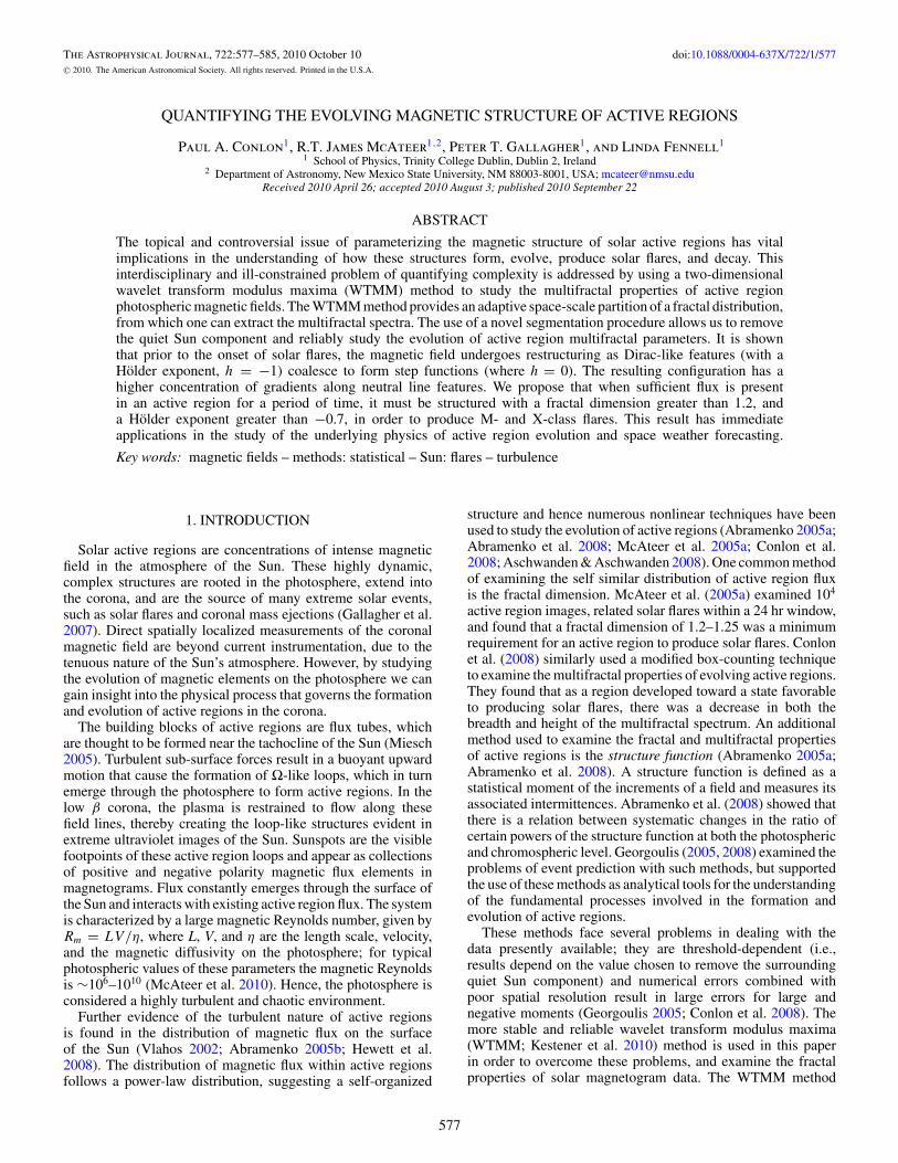
Figure 2 shows NOAA 10488 emerging onto the solar diskon 2003 October 26 and growing rapidly until 2003 October29. Prior to the emergence of the region only a small number ofgradients exceed the thresholds used in segmenting the quiet Sunfeatures, resulting in small and poorly resolved values for D(h).During the emergence period, the Holder exponent increases asa larger number of skeletal gradients pass the segmentationthresholds. The region produced several flares during twoperiods of activity. The first 24 hr period of solar flares startedaround 14:00 UT on 2003 October 27 and contained fiveC-class flares and an M1.9 flare. The second period startedaround 18.00 UT on the 2003 October 29, lasted for two days and

580 CONLON ET AL. Vol. 722

Figure 2. Evolution of NOAA 10488. Top panel: MDI magnetogram images for NOAA 10488 times shown above. Second panel: total area (Mm2). Third panel:total unsigned magnetic flux (Mx). Fourth panel: h for q = 0. Bottom panel: D(h) for q = 0. Associated C-class flares are indicated by thin arrows; bolder arrowsindicate M-class flares. Vertical dotted lines indicate the time of MDI magnetograms of the top row. Dashed horizontal line in the fourth panel is at h = −0.7, a newproposed lower threshold for solar flare production. Dashed horizontal line in the bottom panel highlights a previously proposed threshold of D(h) = 1.2 for solarflare production (McAteer et al. 2005a). All vertical axes in each of the following Figures 3–7 have the same scaling for direct comparison.

resulted in eight C-class flares and two M-class flares. Flaringperiods are associated with a fractal dimension above 1.2 anda Holder exponent greater than that calculated for quiet-Sunfeatures, h > −0.7 (Kestener et al. 2010). This suggests areorganization of the underlying magnetic field. It should benoted that h = −1 corresponds to Dirac white noise, h = 0 astep function, and h = 1 a smooth differential function. As theHolder exponent increases, Dirac-like gradients are replaced bymore structured step-function-like gradients. The formation oflarge structured gradients in the region allows for the storageand release of larger amounts of free magnetic energy.

Figure 3 shows NOAA 10763 rotating into view on 2005May 15 after which both the area and magnetic flux remainedrelatively stable. Around 2005 May 15 17:00 UT the regionentered a period of solar flare productivity, releasing twelveC-class and four M-class flares. During this flaring periodthe fractal dimension and Holder exponent were around or abovethe proposed thresholds for flaring. Some small changes in theHolder exponent seem to be associated with these flares. Priorto some flares there is an increase in the Holder exponent,with a subsequent dip following the flare. This dip in theHolder exponent can be understood as the loss of coherentstructure among the magnetic gradients present in the region ora reduction in the amount of magnetic free energy in the region.The subsequent rise in the Holder exponent and clustering of

the gradients in the region into a coherent structure accompaniesthe release of an M-class flare.

Figure 4 shows NOAA 9878, which rotated onto the solar diskon 2002 March 22 as a fully developed, large, stable region. Theregion produced four C-class flares over a 36 hr period beginningaround 10:00 UT on 2002 March 25. Similarly to NOAA 10763and NOAA 10488, this period of solar flares is associated witha fractal dimension greater than 1.2 and an increase in theHolder exponent to above −0.7. After this period of solar flares,the Holder exponent and fractal dimension decreased to quietSun levels, accompanying the decrease in magnetic free energyavailable in the region.

It is well established that solar flares are associated with ac-tive regions that are large in area and magnetic field strength.However, these examples show that solar flares are also asso-ciated with an increased fractal dimension (D(h) > 1.2) andHolder exponent (h > −0.7). In the following section, we de-scribe active regions which do not produce solar flares, in orderto corroborate these results.

4.2. Non-flaring Regions

Figure 5 shows NOAA 10954 as it emerged on 2007 April28 and rotated across the disk before decaying on 2007 May 5.This was a small region with a maximum area of ∼4×103 Mm2

and maximum flux of ∼7 × 1021 Mx.

No. 1, 2010 QUANTIFYING THE EVOLVING MAGNETIC STRUCTURE OF ACTIVE REGIONS 581

Figure 3. Evolution of NOAA 10763. Top panel: MDI magnetogram images for NOAA 10763 at the times shown. Second panel: total area (Mm2). Third panel: totalunsigned magnetic flux (Mx). Fourth panel: h for q = 0. Bottom panel: D(h) for q = 0. Associated C-class flares are indicated by thin arrows; bolder arrows indicateM-class flares. Vertical dotted lines indicate the time of MDI magnetograms and horizontal lines are proposed thresholds for solar flare production.

The region maintained a high Holder exponent and fractaldimension, indicating a possibility of solar flares, but did notproduce any flares. This demonstrates that fractal propertiesalone are not reliable for the prediction of flares and otherphysical properties, such as area and total magnetic fieldstrength, must be taken into account.

Figure 6 shows NOAA 10942, a small region of maximumarea of around 5×103 Mm2 and a field strength of 9×1021 Mx,which emerged on 2007 February 17. The Holder exponentremains above the proposed threshold of h > −0.7. However,the fractal dimension only briefly rises above the proposedthreshold of D(h) > 1.2. This suggests that although the regionwas structured in a manner favorable to flaring (large Holderexponent), the region was not large enough (in area or flux) orconcentrated enough (as indicated by the low fractal dimension)in order to store sufficient magnetic energy for solar flares.

Figure 7 shows NOAA 10956, which rotated around the eastlimb on 2007 May 15. Apart from a C-class flare while onthe limb, the region produced no further flares. The magneticflux reached a peak of 1 × 1022 Mx and the area peaked at3×104 Mm2. Given the large amount of magnetic flux present in

the region, the occurrence of solar flares was likely. However, asthe Holder exponent oscillates around the proposed threshold,and the fractal dimension remains below, the region is neverstructured in a manner favorable to producing solar flares.

These results show that even in active regions seeminglycontaining sufficient flux, the magnetic field must be structuredin a sufficiently complex configuration in order to produceflares. Similarly, a complex configuration is insufficient by itself(without a large flux), to produce flares. In the three activeregions studied here, one of either the magnetic flux, fractaldimension, or Holder exponent is too small and so no solarflares occur.

5. CONCLUSIONS AND FUTURE WORK

The WTMM method is shown to be a stable and accuratemathematical tool for the analysis of magnetic fields on thesolar disk. The WTMM method allows for the calculation ofthe magnetic field fractal dimension and Holder exponent basedon the distribution of gradients within the magnetic structureacross scale space. The segmentation of quiet Sun magnetic

582 CONLON ET AL. Vol. 722

Figure 4. Evolution of NOAA 9878. Top panel: MDI magnetogram image for NOAA 9878 at the times shown. Second panel: total area (Mm2). Third panel: totalunsigned magnetic flux (Mx). Fourth panel: h for q = 0. Bottom panel: D(h) for q = 0. Associated C-class flares are indicated by thin arrows; bolder arrows indicateM-class flares. Vertical dotted lines indicate the time of MDI magnetograms and horizontal lines are proposed thresholds for solar flare production

information in gradient space allows for the sole study of eachactive region without the introduction of artifacts associated withthresholding. Table 1 outlines our results and shows a strong linkbetween size, complexity, and solar flares. Similar to the resultsof McAteer et al. (2005a), a lower threshold in of D(h) > 1.2is found to be a necessary but insufficient condition for theoccurrence for solar flares. We propose a further constraint of aHolder exponent of no less than −0.7 as an indicator of the futureoccurrence of solar flares. The Holder exponent detects therestructuring of active regions from a field representing Dirac-like gradients toward one closer to step-function-like gradients.Thus, if a region is sufficiently large in both area and flux, andhas a sufficiently high fractal dimension and Holder exponent,the possibility of the region producing solar flares is greatlyincreased.

It is clear that the fractal dimension and Holder exponentoffer great insight into the structure of active regions, however acautionary note is necessary as this small sample size restricts usto only qualitative statements regarding solar flare probabilities.As suggested by McAteer et al. (2010), the likely nonlinearnature of the driver of flares (i.e., reconnection) combined

with the unknown exact link between the location of themeasurements (i.e., the photosphere) and the location of theevent (i.e., the corona) may make reliable solar flare predictionsan almost impossible task. However, the results presentedhere do confirm the ability of multiscale methods to detectcharacteristic changes in magnetic elements on the photosphereof the Sun (Hewett et al. 2008; Abramenko 2005b). In particular,those characteristics such as changes in the flatness of structurefunctions, the dimensional and contribution diversity of themultifractal spectrum, and the fractal dimension (Abramenko2005a; Conlon et al. 2008; McAteer et al. 2005a) are associatedwith an enhanced probability of producing flares. The workpresented here is an improvement on each of these methods andallows for a more detailed analysis than was previously possibleof the processes involved in the evolution of active regions.

There are several remaining weak points in this method.While the best effort has been made to remove the quiet Suncomponent, this problem remains open to interpretation. Ourchosen value of 40, used to threshold the wavelet transformmodulus gradients at the smallest scale, was chosen so as tomaximize the contribution of gradients associated with active

No. 1, 2010 QUANTIFYING THE EVOLVING MAGNETIC STRUCTURE OF ACTIVE REGIONS 583

Figure 5. Evolution of NOAA 10954. Top panel: MDI magnetogram image for NOAA 10954 at the times shown. Second panel: total area (Mm2). Third panel: totalunsigned magnetic flux (Mx). Fourth panel: h for q = 0. Bottom panel: D(h) for q = 0. Vertical dotted lines indicate the time of MDI magnetograms and horizontallines are proposed thresholds for solar flare production

regions and minimize the number associated with quiet Sunfeatures. Active regions of all sizes contain a large number oflow strength gradients. As such, the incorporation of the slopethreshold in modulus space may reduce the number of theselow strength gradients in the calculations. Given the ranges ofscales present in active regions these results are also limited bythe use of an arbitrary and fixed regression range. While greatcare has been taken to select the most appropriate range of scalesfor each image, an automated regression technique is required toimprove on these results. Furthermore, it is unclear how changesin the resolution of magnetogram images will affect the differentmethods used to calculate the multifractal parameters of activeregion. As the WTMM method calculates these parametersbased on the distribution of gradients within the image, it shouldbe more robust to changes in resolution (as compared to thetraditional box-counting method). The enhanced detail offeredby an increase in resolution would increase the number of visiblegradients within the images and hence remove the need for arunning average of magnetograms.

These results represent only one data point in the multifrac-tal spectrum, the so-called fractal dimension or q = 0. TheWTMM method allows for the calculation and analysis of thefull multifractal spectrum. This is akin to performing traditionalemission-line spectroscopy, studying the amplitude and wave-length of the peak, but ignoring the width and asymmetry be-tween the wings. As such, a future investigation into the behaviorof the whole spectrum will provide additional information intothe changing structure of active region magnetic fields. Giventhe results of Conlon et al. (2008), changes in the full multifrac-tal spectrum may provide a clearer distinction between flaringand non-flaring regions. Taken together with other physical pa-rameters, the multifractal spectrum may make it possible todetect the restructuring of active region magnetic fields prior toflaring. Further work is needed on a larger set of active regions(McAteer et al. 2005b; Higgins et al. 2010) to fully access thecapability of the WTMM method in order to detect the condi-tions favorable for flaring and further constrain any thresholdsthat may or may not exist.

584 CONLON ET AL. Vol. 722

Figure 6. Evolution of NOAA 10942. Top panel: MDI magnetogram image for NOAA 10942 at the times shown. Second panel: total area (Mm2). Third panel: totalunsigned magnetic flux (Mx). Fourth panel: h for q = 0. Bottom panel: D(h) for q = 0. Vertical dotted lines indicate the time of MDI magnetograms and horizontallines are proposed thresholds for solar flare production

Table 1Summary of Results for the Six Active Regions Studied

NOAA Total Area Magnetic Flux Fractal Dimension Holder Exponent FlaresAR (Mm2) (1022 Mx)

10488 22921 9.95 1.88 0.10 13 C & 3 M10763 11482 2.40 1.38 −0.43 12 C & 4 M9878 23415 5.48 1.34 −0.42 4 C10954 X X X −0.58 X10942 X X X −0.56 X10956 13522 2.26 X X X

Note. Maximum values for the total area, magnetic flux, Fractal Dimension, and Holder exponent are presentedwhen they exceed thresholds for an extended period of time.

The authors acknowledge the helpful advice and supportof Dr. Kestener, Dr. Khalil, and Dr. Arneodo, along withDr. Georgoulis and Dr. Abramenko for several fruitful dis-cussions on this topic, and the referee and editor for sug-gesting several useful changes to the manuscript. The au-

thors thank the SOHO/MDI consortia for their data. SOHOis a joint project by ESA and NASA. This research was sup-ported by a grant from the “Ulysses–Ireland–France ExchangeScheme” operated by the Royal Irish Academy and the Ministeredes Affaires Etrangeres. P.A.C. is an IRCSET Government of

No. 1, 2010 QUANTIFYING THE EVOLVING MAGNETIC STRUCTURE OF ACTIVE REGIONS 585

Figure 7. Evolution of NOAA 10956. Top panel: MDI magnetogram image for NOAA 10956 on at the times shown. Second panel: total area (Mm2). Third panel: totalunsigned magnetic flux (Mx). Fourth panel: h for q = 0. Bottom panel: D(h) for q = 0. Vertical dotted lines indicate the time of MDI magnetograms, the associatedC-class flare is indicated by the thin arrow, and horizontal lines are proposed thresholds for solar flare production.

Ireland Scholar. R.T.J.M. is PI of a Marie Curie Fellowshipunder FP6.

REFERENCES

Abramenko, V., Yurchyshyn, V., & Wang, H. 2008, ApJ, 681, 1669Abramenko, V. I. 2005a, Sol. Phys., 228, 29Abramenko, V. I. 2005b, ApJ, 629, 1141Arneodo, A., Decoster, N., & Roux, S. G. 2000, Eur. Phys. J. B, 15, 567Aschwanden, M. J., & Aschwanden, P. D. 2008, ApJ, 674, 530Bugayevskiy, L. M., & Snyder, J. P. 1995, Map Projections: A Reference Manual

(London: Taylor and Francis)Conlon, P. A., Gallagher, P. T., McAteer, R. T. J., Ireland, J., Young, C. A.,

Kestener, P., Hewett, R. J., & Maguire, K. 2008, Sol. Phys., 248, 297Domingo, V., Fleck, B., & Poland, A. I. 1995, Sol. Phys., 162, 1Gallagher, P. T., McAteer, R. T. J., Young, C. A., Ireland, J., Hewett, R. J., &

Conlon, P. 2007, in Space Weather: Research Towards Applications in Europe2nd European Space Weather Week (ESWW2), ed. J. Lilensten (Astrophysicsand Space Science Library, Vol. 344 (Dordrecht: Springer)), 15

Georgoulis, M. K. 2005, Sol. Phys., 228, 5Georgoulis, M. K. 2008, Geophys. Res. Lett., 35, 6

Hewett, R. J., Gallagher, P. T., McAteer, R. T. J., Young, C. A., Ireland, J.,Conlon, P. A., & Maguire, K. 2008, Sol. Phys., 248, 311

Higgins, P., Bloomfield, D., McAteer, R. J., & Gallagher, P. T. 2010, Adv. SpaceRes., doi:10.1016/j.asr.2010.06.024

Ireland, J., Young, C. A., McAteer, R. T. J., Whelan, C., Hewett, R. J., &Gallagher, P. T. 2008, Sol. Phys., 252, 121

Kestener, P., Conlon, P., Khalil, A., Fennell, L., McAteer, R., Gallagher, P., &Arneodo, A. 2010, ApJ, 717, 995

McAteer, R. J., Gallagher, P. T., & Conlon, P. A. 2010, Adv. Space Res., 45,1067

McAteer, R. T. J., Gallagher, P. T., & Ireland, J. 2005a, ApJ, 631,628

McAteer, R. T. J., Gallagher, P. T., Ireland, J., & Young, C. A. 2005b, Sol. Phys.,228, 55

McAteer, R. T. J., Kestener, P., Arneodo, A., & Khalil, A. 2010, Sol. Phys., 262,387

McAteer, R. T. J., Young, C. A., Ireland, J., & Gallagher, P. T. 2007, ApJ, 662,691

Miesch, M. S. 2005, Living Rev. Solar Phys., 2, 1Scherrer, P. H., et al. 1995, Sol. Phys., 162, 129Vlahos, L. 2002, in SOLMAG 2002: Proc. Magnetic Coupling of the Solar At-

mosphere Euroconference, ed. H. Sawaya-Lacoste (ESA Special Publication,Vol. 505; Noordwijk: ESA), 105