Online Statistical Inference for QuantifyingMandible Growth in CT Images

Moo K. Chung1,2, Ying Ji Chuang2, Houri K. Vorperian2

1Department of Biostatistics and Medical Informatics2Vocal Tract Development Laboratory, Waisman Center

University of Wisconsin-Madison, USA

mkchung@wisc.edu

Abstract. We present a unified online statistical framework for quan-tifying a collection of binary segmentation of mandibles in CT images.Since the segmentation was done semi-automatically, the processed bi-nary images were available in a sequential manner. Thus, there was aneed to develop an iterative analysis framework where the final statis-tical maps are updated sequentially each time a new image is added tothe analysis. The proposed method is applied to identify and characterizeregions of mandible growth during the first two decades of life.

1 Introduction

The typical implementation of statistical inference in medical imaging requiresthat all the images are available in advance. That is the usual premise of existingmedical image analysis tools such as ImageJ, SPM, SFL and AFNI. However,there are many situations where the entire imaging dataset is not available andparts of imaging data are obtained in a delayed sequential manner. This is acommon problem in medical imaging, where not every subject is scanned andprocessed at the same time.

When the image size is large, it may not be possible to fit all of the imag-ing data in a computer’s memory, making it necessary to perform the analysisby adding one image at a time in a sequential manner. In another situation,the imaging dataset may be so large that it is not practical to use all the im-ages in the dataset but use a subset of the dataset. In this situation, we needto incrementally add stratified datasets one at a time to see if we are achiev-ing reasonable statistical results. In all the above situations, we need a way toincrementally update the analysis result without repeatedly running the entireanalysis whenever new images are added.

An online algorithm is one that processes its inputted data in a sequentialmanner [8]. Instead of processing the entire set of imaging data from the start,an online algorithm processes one image at a time. That way, we can bypassthe memory requirement, reduce numerical instability and increase computa-tional efficiency. Online algorithms and machine learning are both concernedwith problems of making decisions about the present based on knowledge of the

2

past [3]. Thus, online algorithms are often encountered in machine learning lit-erature but there is very limited number of studies in medical imaging possiblydue to the lack of problem awareness. With the ever-increasing amount of largescale medical imaging database such as Alzheimer’s disease neuroimaging initia-tive (ADNI) and human connectome project (HCP), the development of variousonline algorithm is warranted. Motivated by the concept of online algorithms inmachine learning, we propose to develop online statistical inference procedures.The methods are then used in characterizing the mandible growth using binarymandible segmentations from CT.

2 Probabilistic model of binary segmentation

Let p(x) be the probability of voxel x belonging to some region of interest (ROI)M. Let 1M be an indicator function defined as 1M(x) = 1 if x ∈ M and 0otherwise. We assume that the shape of M is random (due to noise) and weassociate it with probability p(x):

P (x ∈M) = p(x), P (x /∈M) = 0.

The volume of M given by vol(M) =∫R3 1M(x) dx. is also random. The mean

volume of M is then

E vol(M) =

∫R3

E 1M(x) dx =

∫R3

p(x) dx.

The integral of the probability map thus can be used as an estimate for thevolume of ROI. Unfortunately, mandible segmentations often have holes andcavities that have to be patched topologically for accurate volume estimation(Fig. 1-a). Such topological defects can be easily patched by Gaussian kernelsmoothing (Fig. 1-b) without resorting to more complicated topology correctionmethods [5].

Consider a 3-dimensional Gaussian kernel

K(x) =1

(2π)3/2exp

(− ‖x‖

2

2

),

where ‖ · ‖ is the Euclidean norm of x ∈ R3. The rescaled kernel Kt is defined as

Kt(x) =1

t3K(xt

).

Gaussian kernel smoothing applied to the probability map p(x) is given by

Kt ∗ p(x) =

∫R3

Kt(x− y)p(y) dy. (1)

The volume estimate is invariant under smoothing:

E vol(M) =

∫R3

p(y) dy

=

∫R3

∫R3

Kt(x− y)p(y) dy dx =

∫R3

Kt ∗ p(x) dx.

3

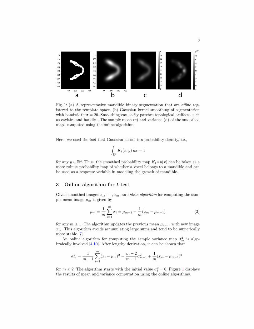
Fig. 1: (a) A representative mandible binary segmentation that are affine reg-istered to the template space. (b) Gaussian kernel smoothing of segmentationwith bandwidth σ = 20. Smoothing can easily patches topological artifacts suchas cavities and handles. The sample mean (c) and variance (d) of the smoothedmaps computed using the online algorithm.

Here, we used the fact that Gaussian kernel is a probability density, i.e.,∫R3

Kt(x, y) dx = 1

for any y ∈ R3. Thus, the smoothed probability map Kt ∗p(x) can be taken as amore robust probability map of whether a voxel belongs to a mandible and canbe used as a response variable in modeling the growth of mandible.

3 Online algorithm for t-test

Given smoothed images x1, · · · , xm, an online algorithm for computing the sam-ple mean image µm is given by

µm =1

m

m∑i=1

xi = µm−1 +1

m(xm − µm−1) (2)

for any m ≥ 1. The algorithm updates the previous mean µm−1 with new imagexm. This algorithm avoids accumulating large sums and tend to be numericallymore stable [7].

An online algorithm for computing the sample variance map σ2m is alge-

braically involved [4,10]. After lengthy derivation, it can be shown that

σ2m =

1

m− 1

m∑i=1

(xi − µm)2 =m− 2

m− 1σ2m−1 +

1

m(xm − µm−1)2

for m ≥ 2. The algorithm starts with the initial value σ21 = 0. Figure 1 displays

the results of mean and variance computation using the online algorithms.

4

For comparing a collection of images between groups, two-sample t-statisticcan be used. Given measurements x1, · · · , xm ∼ N(µ1, (σ1)2) in one group andy1, · · · , yn ∼ N(µ1, (σ2)2) in the other group, the two-sample t-statistic for test-ing H0 : µ1 = µ2 at each voxel x is given by

Tm,n(x) =µ1m − µ2

n − (µ1 − µ2)√(σ1)2m/m+ (σ2)2n/n

, (3)

where µ1m, µ

2n, (σ1)2m, (σ

2)2m are sample means and variances in each group esti-mated using the online algorithm. Tm,n is then sequentially computed as

T1,0 → T2,0 → · · · → Tm,0 → Tm,1 → · · · → Tm,n

in m+ n steps.

4 Online algorithm for linear regression

The online algorithm for linear regression is itself useful but additionally moreuseful in constructing an online algorithm for F -tests in the next section. Givendata vector ym−1 = (y1, · · · , ym−1)′ and design matrix Zm−1, consider linearmodel

ym−1 = Zm−1λm−1 (4)

with unknown parameter vector λm−1 = (λ1, λ2, · · · , λk)′. Multiplying Z ′m−1 onthe both sides we have

Z ′m−1ym−1 = Z ′m−1Zm−1λm−1 (5)

Let Wm−1 = Z ′m−1Zm−1, which is a k × k matrix. In most applications, thereare substantially more data than the number of parameters, i.e., m � k, andWm−1 is invertible. The least squares estimation (LSE) of λm−1 is given by

λm−1 = W−1m−1Z′mym−1.

When new data ym is introduced to the linear model (4), the model is updatedto (

ym−1ym

)=

(Zm−1zm

)λm,

where zm is 1× k row vector. Subsequently, we have

W ′m−1λm−1 + z′mym = (Wm−1 + z′mzm)λm.

Using Woodbury formula [6],

(Wm−1 + z′mzm)−1 = W−1m−1 − cmW−1m−1z

′m,

5

where cm = 1/(1 + zmWm−1z′m) is scalar. Then we have the explicit online

algorithm for updating the parameter vector:

λm = (I −W−1m−1z′mym − cmW−1m−1z

′mW

′m−1)λm−1 − cmW−1m−1z

′mz′mym, (6)

where I is the identity matrix of size k × k. Since the algorithm requires Wm−1to be invertible, the algorithm must start from

λk → λk+1 → · · · → λm.

At each iteration, we need to store k× k matrix Wm−1. In many applications, kwill not be larger than 10 and most likely around 5 or less, which is manageableas far as computer memory is concerned.

5 Online algorithm for F -test

Let yi be the i-th image, xi = (xi1, · · · , xip)′ to be the variables of interest andzi = (zi1, · · · , zik)′ to be nuisance covariates corresponding to the i-th image.We assume there are m−1 images to start with. Consider a general linear model

ym−1 = Zm−1λm−1 +Xm−1βm−1,

where Zm−1 = (zij) is (m− 1)× k design matrix, Xm−1 = (xij) is (m− 1)× pdesign matrix. λm−1 = (λ1, · · · , λk)′ and βm−1 = (β1, · · · , βp)′ are unknown pa-rameter vectors to be estimated at the (m−1)-th iteration. Consider hypotheses

H0 : β = 0 vs. H1 : β 6= 0.

The reduced null model when β = 0 is ym−1 = Zm−1λ0m−1. The goodness-of-fit

of the null model is measured by the sum of the squared errors (SSE):

SSE0m−1 = (ym−1 − Zm−1λ

0m−1)′(ym−1 − Zm−1λ

0m−1),

where λ0m−1 is estimated using the online algorithm (6). This provide the se-

quential update of SSE under H0:

SSE0k → SSE0

k+1 → · · · → SSE0m.

Similarly the fit of the alternate full model is measured by

SSE1m−1 = (ym−1 − Zm−1γ

1m−1)′(ym−1 − Zm−1γ

1m−1),

where Zm−1 = [Zm−1Xm−1] is the combined design matrix and

γ1m−1 =

(λ1m−1β1m−1

)is the combined parameter vector. Similarly SSE under H1 is given as

SSE1k+p → SSE1

k+1 → · · · → SSE1m.

Under H0, the test statistic at the m-th iteration fm is given by

fm =(SSE0 − SSE1)/p

SSE0/(m− p− k)∼ Fp,m−p−k, (7)

which is the F -statistic with p and m− p− k degrees of freedom.

6

6 Random field theory

Since the statistic maps are correlated over voxels, it is necessary to correctmultiple comparisons using the random field theory [11], which is based on theexpected Euler characteristic (EC) approach. Given statistic maps S such as t-or F -test maps, for sufficiently high threshold h, we have

P(

supx∈M

S(x) > h)

=

N∑d=0

µd(M)ρd(h), (8)

where µd(M) is the d-th Minkowski functional or intrinsic volume of M. ρd(h)is the EC-density of S. The explicit formulas for µd and ρd are given in [11].

7 Application

Subjects. The dataset consisted of 290 typically developing individuals rangingin age from birth to 20 years old. Only CT images showing the full mandiblewithout any motion or any other artifacts were selected though minimal dentalartifacts were tolerated. The age distribution of the subjects is 9.66±6.34 years.The minimum age was 0.17 years and maximum age was 19.92 years. A totalof 160 male and 130 female subjects were divided into 3 groups. Group I (agebelow 7) contained 130 subjects. , Group II (between 7 and 13) contained 48subjects. Group III (between 13 and 20) contained 112 subjects.

Image preprocessing. CT images were visually inspected and determined to cap-ture the whole mandible geometry. The mandibles in CT were semi-automaticallysegmented using an in-house processing pipeline that involves image intensitythresholding using the Analyze software package (AnalyzeDirect, Inc., OverlandPark, KS). Each of the processed mandibles were examined visually and editedmanually by raters. The segmented binary images were then affine registeredto the mandible labeled as F226-15-04-002-M using the Advanced Normaliza-tion Tools (ANTS) [2] (Fig. 1). The mandible F226-15-04-002-M served as thetemplate. Due to the lack of existing prior map in the field, we simply used thenormalized binary segmentation results as the probability map p(x).

CT images are inherently noisy due to errors associated with image acquisi-tion. Compounding the image acquisition errors, there are errors caused by imageregistration and semiautomatic segmentation. So it is necessary to smooth outthe affine registered segmented images. We smoothed the binary images withGaussian kernel with bandwidth σ = 20 voxels (Fig. 1). The average of all 290smoothed binary images was computed and used as the final template where theonline statistical analyses are performed. For visualization, the statistical mapsare projected onto the surface of template.

Age effects. We performed the t-test to assess age effects between the groups.The resulting t-statistic maps are displayed in Fig. 2-top. Voxels above or below

7

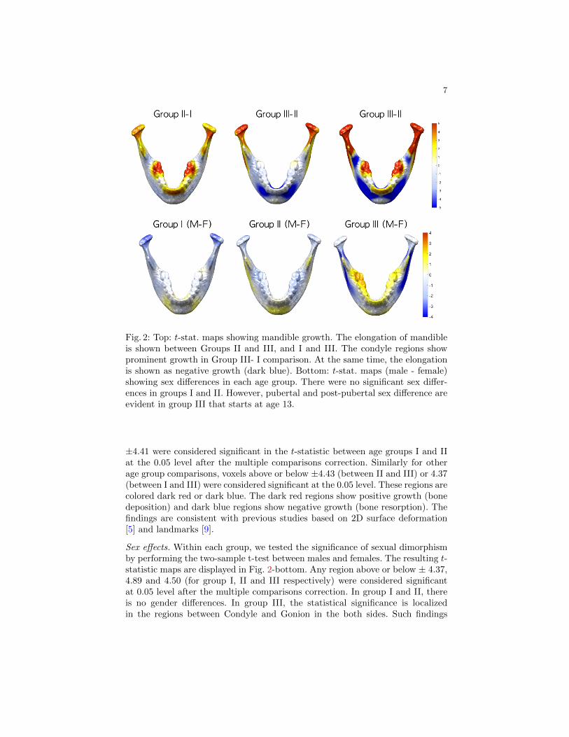
Fig. 2: Top: t-stat. maps showing mandible growth. The elongation of mandibleis shown between Groups II and III, and I and III. The condyle regions showprominent growth in Group III- I comparison. At the same time, the elongationis shown as negative growth (dark blue). Bottom: t-stat. maps (male - female)showing sex differences in each age group. There were no significant sex differ-ences in groups I and II. However, pubertal and post-pubertal sex difference areevident in group III that starts at age 13.

±4.41 were considered significant in the t-statistic between age groups I and IIat the 0.05 level after the multiple comparisons correction. Similarly for otherage group comparisons, voxels above or below ±4.43 (between II and III) or 4.37(between I and III) were considered significant at the 0.05 level. These regions arecolored dark red or dark blue. The dark red regions show positive growth (bonedeposition) and dark blue regions show negative growth (bone resorption). Thefindings are consistent with previous studies based on 2D surface deformation[5] and landmarks [9].

Sex effects. Within each group, we tested the significance of sexual dimorphismby performing the two-sample t-test between males and females. The resulting t-statistic maps are displayed in Fig. 2-bottom. Any region above or below ± 4.37,4.89 and 4.50 (for group I, II and III respectively) were considered significantat 0.05 level after the multiple comparisons correction. In group I and II, thereis no gender differences. In group III, the statistical significance is localizedin the regions between Condyle and Gonion in the both sides. Such findings

8

are consistent with general findings on sexual dimorphism that become evidentduring puberty.

8 Discussion

The image processing and analysis somewhat resembles the voxel-based mor-phometry (VBM) widely used in modeling the gray and white matter tissueprobability maps in structural brain magnetic resonance imaging studies [1]. InVBM, the posterior probability map is estimated using the prior probabilitymap. However, there is no such prior map in mandibles CT studies yet. Our290 subject average probability map is distributed as a potential prior map forresearchers [web address blinded]. Although VBM was originally developed forwhole brain MRI, we have demonstrated similar approach can be successfullyapplied to mandible bone growth analysis.

To address the issue of incrementally available imaging database as well ascomputational burden for large-scale images, we have developed online algo-rithms for various statistical test procedures. It is hoped that this study moti-vates imaging researchers to develop online algorithms for more complex statis-tical inference procedures.

References

1. J. Ashburner and K. Friston. Why voxel-based morphometry should be used.NeuroImage, 14:1238–1243, 2001.

2. B.B. Avants, C.L. Epstein, M. Grossman, and J.C. Gee. Symmetric diffeomorphicimage registration with cross-correlation: Evaluating automated labeling of elderlyand neurodegenerative brain. Medical Image Analysis, 12:26–41, 2008.

3. A. Blum. On-line algorithms in machine learning. In Online algorithms, pages306–325. Springer, 1998.

4. T.F. Chan, G.H. Golub, and R.J. LeVeque. Algorithms for computing the samplevariance: Analysis and recommendations. The American Statistician, 37:242–247,1983.

5. M.K. Chung, A. Qiu, S. Seo, and H.K. Vorperian. Unified heat kernel regressionfor diffusion, kernel smoothing and wavelets on manifolds and its application tomandible growth modeling in CT images. Medical Image Analysis, 22:63–76, 2015.

6. C.Y. Deng. A generalization of the Sherman–Morrison–Woodbury formula. AppliedMathematics Letters, 24:1561–1564, 2011.

7. T. Finch. Incremental calculation of weighted mean and variance. University ofCambridge, 4:11–5, 2009.

8. R.M. Karp. On-line algorithms versus off-line algorithms: How much is it worthto know the future? In IFIP Congress, volume 12, pages 416–429, 1992.

9. M.P. Kelly, H.K. Vorperian, Y. Wang, K.K. Tillman, H.M. Werner, M.K. Chung,and L.R. Gentry. Characterizing mandibular growth using three-dimensional imag-ing techniques and anatomic landmarks. Archives of Oral Biology, 2017.

10. D. Knuth. The art of computing, vol. ii: Seminumerical algorithms, 1981.11. K.J. Worsley, J. Cao, T. Paus, M. Petrides, and A.C. Evans. Applications of

random field theory to functional connectivity. Human Brain Mapping, 6:364–7,1998.