Statistical Methods in Modulation Classification
91
Transcript of Statistical Methods in Modulation Classification
TAMPERE UNIVERSITY OF TECHNOLOGYDEPARTMENT OF INFORMATION TECHNOLOGY
Antti-Veikko Rosti
STATISTICAL METHODS INMODULATION CLASSIFICATION
MASTER OF SCIENCE THESIS
SUBJECT APPROVED BY DEPARTMENTALCOUNCIL ON December 9, 1998Examiners: Prof. Visa Koivunen
Lic. Tech. Jukka Mannerkoski
Preface
The research and study presented in this thesis was carried out in the SignalProcessing Laboratory of Tampere University of Technology.I would like to thank Professor Visa Koivunen, my advisor and examiner, for hisvaluable guidance in statistical signal processing and making of this thesis. I wouldalso like to thank my other examiner, Lic. Tech. Jukka Mannerkoski, for sharinghis expertise in cyclostationary statistics.I wish to express my gratitude to my colleagues, Mr. Anssi Rämö and Mr. TeemuSaarelainen, for their help in making of this thesis and putting up with me in thesame oce. I am also grateful to Mr. Anssi Huttunen and Mr. Saarelainen fortheir help in proof reading.I would like to thank the people in Signal Processing Laboratory for the pleasantworking environment. Especially I would like to thank Audio Research Group,where I hope to enjoy working in the future.I wish to express my gratitude to my family and friends who have always beenthere for me.
Tampere, June 1, 1999
Antti-Veikko RostiOpiskelijankatu 4 E 29033720 TampereTel. 050-523 7764
ii
Contents
Abstract vi
Tiivistelmä vii
List of Abbreviations viii
List of Symbols x
1 Introduction 1
2 Representation of Communication Signals 32.1 Signal Representation . . . . . . . . . . . . . . . . . . . . . . . . . . 3
2.1.1 Analytic Signal . . . . . . . . . . . . . . . . . . . . . . . . . 42.1.2 Complex Envelope . . . . . . . . . . . . . . . . . . . . . . . 6
2.2 Analog Modulation . . . . . . . . . . . . . . . . . . . . . . . . . . . 82.2.1 Amplitude Modulation . . . . . . . . . . . . . . . . . . . . . 92.2.2 Double-Sideband Modulation . . . . . . . . . . . . . . . . . 102.2.3 Single-Sideband Modulation . . . . . . . . . . . . . . . . . . 122.2.4 Frequency Modulation . . . . . . . . . . . . . . . . . . . . . 142.2.5 Phase Modulation . . . . . . . . . . . . . . . . . . . . . . . . 16
2.3 Digital Modulation . . . . . . . . . . . . . . . . . . . . . . . . . . . 172.3.1 Amplitude Shift Keying . . . . . . . . . . . . . . . . . . . . 182.3.2 Phase Shift Keying . . . . . . . . . . . . . . . . . . . . . . . 202.3.3 Quadrature Amplitude Modulation . . . . . . . . . . . . . . 212.3.4 Frequency Shift Keying . . . . . . . . . . . . . . . . . . . . . 23
iii
3 Statistical Tools 253.1 Random Processes . . . . . . . . . . . . . . . . . . . . . . . . . . . 25
3.1.1 Stationary Processes . . . . . . . . . . . . . . . . . . . . . . 273.1.2 Cyclostationary Processes . . . . . . . . . . . . . . . . . . . 28
3.2 Higher-Order Statistics . . . . . . . . . . . . . . . . . . . . . . . . . 303.2.1 Higher-Order Moments . . . . . . . . . . . . . . . . . . . . . 313.2.2 Cumulants and Multi-Correlations . . . . . . . . . . . . . . 323.2.3 Higher-Order Spectra . . . . . . . . . . . . . . . . . . . . . . 36
4 Review of Modulation Classication 384.1 Maximum Likelihood Approach . . . . . . . . . . . . . . . . . . . . 38
4.1.1 General Maximum Likelihood Methods . . . . . . . . . . . . 394.1.2 MPSK Classier Based on the Exact Phase Distribution . . 394.1.3 Classiers Based on the Likelihood Functions . . . . . . . . 404.1.4 Maximum Likelihood Classier for CPM . . . . . . . . . . . 42
4.2 Pattern Recognition Approach . . . . . . . . . . . . . . . . . . . . . 424.2.1 Envelope Based Methods . . . . . . . . . . . . . . . . . . . . 434.2.2 Higher-Order Methods . . . . . . . . . . . . . . . . . . . . . 444.2.3 Other Methods . . . . . . . . . . . . . . . . . . . . . . . . . 45
5 Implemented Methods 475.1 Test Signal Generation for the Simulations . . . . . . . . . . . . . . 475.2 Implemented Methods . . . . . . . . . . . . . . . . . . . . . . . . . 48
5.2.1 Ratio of Variance to Squared Mean . . . . . . . . . . . . . . 485.2.2 Deviations in Instantaneous Properties . . . . . . . . . . . . 505.2.3 Even Moments of MPSK Signals . . . . . . . . . . . . . . . 525.2.4 Time-Average of Complex Envelope MFSK Process . . . . . 55
6 Simulation Results 576.1 Results . . . . . . . . . . . . . . . . . . . . . . . . . . . . . . . . . . 57
6.1.1 Ratio of Variance to Squared Mean . . . . . . . . . . . . . . 576.1.2 Deviations in Instantaneous Properties . . . . . . . . . . . . 576.1.3 Even Moments of MPSK Signals . . . . . . . . . . . . . . . 626.1.4 Time-Average of Complex Envelope MFSK Process . . . . . 63
6.2 Discussion on Features . . . . . . . . . . . . . . . . . . . . . . . . . 64
iv

7 Conclusions 66
References 68
A First and Second-Order Statistics of Digital Modulated Signals 72A.1 Carrier Wave . . . . . . . . . . . . . . . . . . . . . . . . . . . . . . 72A.2 Amplitude Shift Keying . . . . . . . . . . . . . . . . . . . . . . . . 73A.3 Phase Shift Keying . . . . . . . . . . . . . . . . . . . . . . . . . . . 75A.4 Frequency Shift Keying . . . . . . . . . . . . . . . . . . . . . . . . . 77
v
TAMPERE UNIVERSITY OF TECHNOLOGYDepartment of Information TechnologySignal Processing LaboratoryRosti, Antti-Veikko: Statistical Methods in Modulation ClassicationMaster of Science Thesis, 71 pages and Appendix, 8 pages.Examiners: Prof. Visa Koivunen and Lic. Tech. Jukka MannerkoskiJune 1999Keywords: modulation classication, cyclostationarity, higher-order statistics
The interest in modulation classication has recently emerged in the research ofcommunication systems. This has been due to the advances in recongurable signalprocessing systems, especially in the study of software radio. Published methodscan be divided into two groups: maximum likelihood and pattern recognitionapproaches. In the maximum likelihood approach, decision rules are often simplebut the test statistics are complicated and assume prior knowledge about thesignals. In the pattern recognition approach, decision rules are often complicatedwhereas the features are simple and fast to calculate.Communication signals contain a vast amount of uncertainty due to the unknownmodulating signal, modulation type, and noise. Therefore the modulation classi-cation problem has to be approached by using statistical methods. The featuresand the test statistics may be derived from the known statistical characteristics ofthe modulated signals. Either implicit or explicit use of higher-order statistics hasbeen studied previously in many communication applications. The higher-orderstatistics are often more preferable because second-order statistics suppress thephase information of the signal. Nevertheless, the estimation of the higher-orderstatistics requires long sample sets and has a high computational complexity. Toovercome these problems, second-order cyclostationary statistics have been studiedand the results seem promising.In this thesis, the feature extraction problem of the modulation classication isdiscussed. Useful characteristics and representations of the communication signalsare presented as well as the relevant knowledge of statistical signal processing. Theprevious methods are presented in a literature review of the modulation classica-tion. The rst and second-order statistics including the cyclostationary statisticsof digital modulated signals are studied, and a novel feature is proposed. Someprevious methods and this novel feature are compared by investigating their dis-crimination performance in Matlab simulations.
vi
TAMPEREEN TEKNILLINEN KORKEAKOULUTietotekniikan osastoSignaalinkäsittelyRosti, Antti-Veikko: Statistical Methods in Modulation ClassicationDiplomityö, 71 s. ja 8 liites.Tarkastajat: Prof. Visa Koivunen ja TkL Jukka MannerkoskiKesäkuu 1999Avainsanat: modulaation luokittelu, syklostationaarisuus, korkeamman asteen tun-nusluvut
Tietoliikennejärjestelmien tutkimuksessa kiinnostus modulaation luokittelua ko-htaan on herännyt viimeaikoina. Tämä johtuu uudelleenkonguroitavien signaalin-käsittelyjärjestelmien kehityksestä ja erityisesti ohjelmistoradion tutkimuksesta.Tunnetut menetelmät voidaan jakaa kahteen ryhmään lähestymistavan perusteel-la: suurimman uskottavuuden estimointiin ja hahmontunnistukseen. Suurimmanuskottavuuden estimaatti voidaan usein päättää helposti mutta testattavat tun-nusluvut ovat monimutkaisia ja signaaleista on tunnettava eräitä ominaisuuksiaetukäteen. Hahmontunnistuksessa päätössäännöt ovat yleensä monimutkaisia mut-ta luokitteluun käytettävät piirteet ovat yksinkertaisia ja voidaan laskea nopeasti.Tietoliikennesignaaleihin liittyy paljon epävarmuutta, koska moduloivaa signaalia,modulaatiotapaa ja kohinaa ei tunneta. Tästä syystä modulaation luokitteluon-gelmaa täytyy käsitellä tilastollisin menetelmin. Piirteet tai testattavat tunnuslu-vut voidaan johtaa moduloitujen signaalien tilastollisista ominaisuuksista. Useissatietoliikennesovelluksissa on tutkittu korkeamman asteen tunnuslukujen käyttöäjoko implisiittisesti tai eksplisiittisesti. Niiden käyttö on suotuisaa, koska toisenasteen tunnusluvut kadottavat signaalin sisältämän vaiheinformaation. Kuitenkinkorkeamman asteen tunnuslukujen estimointi on monimutkaista ja vaatii suurennäytemäärän. Toisen asteen syklostationaarisia tunnuslukuja on tutkittu näidenongelmien välttämiseksi ja tulokset ovat olleet lupaavia.Tässä diplomityössä käsitellään piirteenerotusongelmaa modulaation luokittelussa.Työssä esitetään tietoliikennesignaalien ominaispiirteitä ja signaalien esitystapojasekä tarvittavat tiedot tilastollisesta signaalinkäsittelystä. Kirjallisuusselvityksessäesitellään aiemmin kehitettyjä menetelmiä modulaation luokitteluun. Työssä ontutkittu digitaalisesti moduloitujen signaalien ensimmäisen ja toisen asteen tun-nuslukuja sekä syklostationaarisia tunnuslukuja. Lisäksi esitellään uusi digitaalises-ti moduloitujen signaalien luokitteluun soveltuva piirre. Tämän piirteen ja eräidenkirjallisuudesta löytyvien piirteiden erottelukykyä tutkitaan Matlab-simulaatioilla.
vii
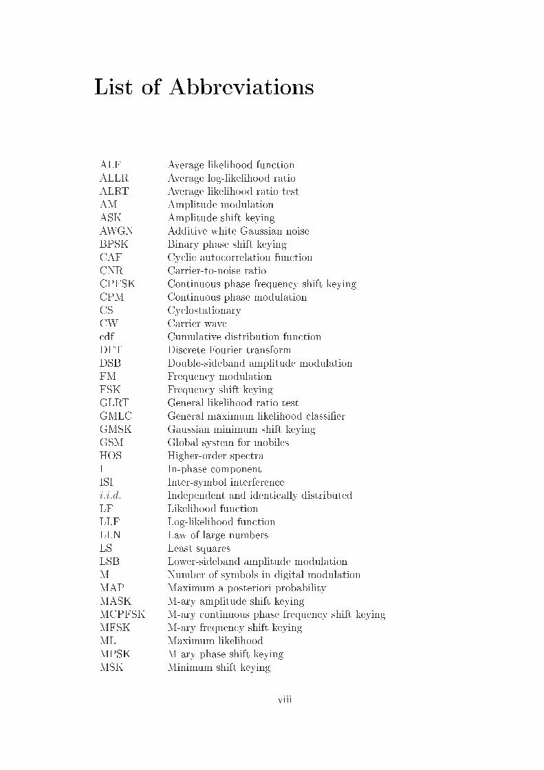
List of Abbreviations
ALF Average likelihood functionALLR Average log-likelihood ratioALRT Average likelihood ratio testAM Amplitude modulationASK Amplitude shift keyingAWGN Additive white Gaussian noiseBPSK Binary phase shift keyingCAF Cyclic autocorrelation functionCNR Carrier-to-noise ratioCPFSK Continuous phase frequency shift keyingCPM Continuous phase modulationCS CyclostationaryCW Carrier wavecdf Cumulative distribution functionDFT Discrete Fourier transformDSB Double-sideband amplitude modulationFM Frequency modulationFSK Frequency shift keyingGLRT General likelihood ratio testGMLC General maximum likelihood classierGMSK Gaussian minimum shift keyingGSM Global system for mobilesHOS Higher-order spectraI In-phase componentISI Inter-symbol interferencei.i.d. Independent and identically distributedLF Likelihood functionLLF Log-likelihood functionLLN Law of large numbersLS Least squaresLSB Lower-sideband amplitude modulationM Number of symbols in digital modulationMAP Maximum a posteriori probabilityMASK M-ary amplitude shift keyingMCPFSK M-ary continuous phase frequency shift keyingMFSK M-ary frequency shift keyingML Maximum likelihoodMPSK M-ary phase shift keyingMSK Minimum shift keying
viii
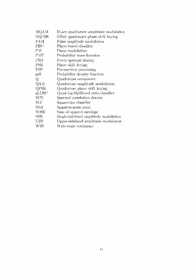
MQAM M-ary quadrature amplitude modulationOQPSK Oset quadrature phase shift keyingPAM Pulse amplitude modulationPBC Phase-based classierPM Phase modulationPMF Probability mass functionPSD Power spectral densityPSK Phase shift keyingPSP Per-survivor processingpdf Probability density functionQ Quadrature componentQAM Quadrature amplitude modulationQPSK Quadrature phase shift keyingqLLRC Quasi log-likelihood ratio classierSCD Spectral correlation densitySLC Square-law classierSNR Signal-to-noise ratioSOSE Sum of squared envelopeSSB Single-sideband amplitude modulationUSB Upper-sideband amplitude modulationWSS Wide-sense stationary
ix
List of Symbols
Modulated SignalsAc Amplitude of carrierA[m] Discrete symbol amplitude sequencea[k] Discrete instantaneous amplitude sequenceacn[k] Normalized centered amplitude sequencea(t) Instantaneous amplitudeC(ω) Spectrum of complex envelopec(t) Complex envelope signalFs Sampling frequencyfc Carrier frequencyf∆ Frequency deviationfN [k] Normalized centered instantaneous frequency sequencef(t) Instantaneous frequencyf [k] Estimated instantaneous frequency sequenceg(t) Signal pulse in digital modulationh(t) Impulse response of a linear lterj Imaginary unitM Number of symbols in digital modulationNs Number of samples in a segmentR(ω) Spectrum of r(t)r[k] Discrete received signal sequencer(t) Received signalr(t) Hilbert transform of r(t)s[m] Discrete symbol sequences(t) Continuous symbol functionT Length of symbol intervalu(t) Unit step functionX(ω) Fourier transform of x(t)x(t) Modulating signalx(t) Time derivative of x(t)v(t) Contribution of additive noise to phase componentw(t) Additive noiseZ(ω) Spectrum of z(t)z(t) Analytic representation of r(t)φ∆ Phase deviationφNL[k] Estimated nonlinear phase component sequenceφuw[k] Unwrapped phase sequenceφ[m] Phase state sequence
x
φ(t) Instantaneous phaseδ(t) Dirac's delta functionµ Modulation indexωc Angular frequency of carrierω(t) Angular frequencyω∆ Angular frequency deviation
Random ProcessesC(t) Random complex envelope processCX
n (ω1, . . . , ωn−1) nth-order polyspectrum of X(t)cXn nth-order cumulant of X
cXn (τ1, . . . , τn−1) nth-order cumulant function of X(t)
cum(·) Cumulant operatorEX [·] Expectation operator with respect to XFX(·) cdf of XfX(·) pdf of XHi Hypothesis number iL(x|Hi) Likelihood function on Hi
MXn (ω1, . . . , ωn−1) nth-order moment spectrum of X
mXn nth-order moment of X
P (·) Probability operatorPX
n (ω1, . . . , ωn−1) nth-order coherency index of Xp(x|Hi) Conditional pdfRX(t1, t2) Autocorrelation function of X(t)RX(τ) Autocorrelation function of WSS process X(t)Rα
X(τ) CAF of X(t)S[m] Random symbol sequenceS(ω) Power spectral densityT Set of real numbersX Random variableX[k] Discrete-time random sequenceX(t) Continuous-time random processx Observationx(t) Sample functionα Cyclic frequencyγX
n nth-order cumulant function of X(t) at originµX(t) Mean function of X(t)σX Standard deviation of Xσ2
X Variance of Xσ2
X(t) Variance function of X(t)Φ[m] Random phase state sequenceΦX(ω) Characteristic function of X(t)ΨX(ω) Cumulative function of X(t)
xi
Featuresmn nth-order moment of instantaneous phaseP Power spectrum symmetry measureR Ratio of variance to squared meanγmax Spectral power density maximumµC Time-average of complex envelopeµa
42 Kurtosis of instantaneous amplitudeµf
42 Kurtosis of instantaneous frequencyσa Standard deviation of instantaneous amplitudeσaa Standard deviation of absolute amplitudeσaf Standard deviation of instantaneous frequencyσap Standard deviation of absolute phaseσdp Standard deviation of direct phase
xii
Chapter 1
Introduction
The interest in modulation classication has been growing since the late eighties upto date. It has several possible roles in both civilian and military applications suchas signal conrmation, interference identication, monitoring, spectrum manage-ment, and surveillance [42]. At the moment, the most attractive application areais software radio and other recongurable communication systems. Modulationclassication is an intermediate step between signal detection and demodulation.In addition to modulation type, some other parameters should be estimated beforesuccessful demodulation.Modulation classiers, like general pattern recognition systems [38], consist of mea-surement, feature extraction, and decision parts. The measurement is obtained bya front-end which will receive the signal of interest and carry out some preprocess-ing such as ltering, down-conversion, equalization, and sampling. The featureextraction part reduces the dimensionality of the measurement by extracting thedistinctive features which should be simple and fast to calculate. There are sev-eral ways to make the decision based on the obtained features such as decisionfunctions, distance functions, and neural networks.The received signal to be classied according to its modulation type contains muchuncertainty which should be encountered by statistical tools. Therefore the knownmethods are based on dierent statistics obtained from the received signal. Thesestatistics can be derived from continuous-time signals and they hold for sampleddiscrete signals which may be processed by some digital device. Some knownmethods are based on the higher-order statistics of the received signal but theyare often very complicated and dicult to obtain [28]. The methods exploiting thecyclostationarity of digital modulated signals have not yet attained much attentionalthough cyclostationary statistics have shown many desirable properties in otherelds of communication systems [13]. There are also many ad-hoc methods whichcan be eventually shown to contain implicit statistical information about the signal.In this study, we have concentrated on the problem of the feature extraction in themodulation classiers. The features are selected for the simulation part accord-ing to their applicability for the modulation types used in radio communication.
CHAPTER 1. INTRODUCTION 2
Therefore the modulation types under concern have a constant envelope and inthe case of digital modulation, small symbol sets. The most of the known methodsare reviewed and a new attractive feature is introduced as a result of studying therst and second-order statistics of digital modulated signals.This thesis consists of seven chapters and one appendix. Useful characteristics andrepresentations of the communication signals are introduced in Chapter 2. Theminimal representation is presented and it is used over the remaining chapters.Each modulation type is reviewed and their key properties are derived to showtheir importance in the modulation classication.Chapter 3 presents the relevant knowledge of the statistics which is necessary todescribe the uncertainty in the received communication signal. The interpretationof random processes is given including stationary and cyclostationary processes.The second part of the chapter is dedicated to higher-order statistics includinghigher-order moments, cumulants, and spectra.Chapter 4 reviews the previous methods found in literature and publications. Thereviewed methods have been divided into two groups according to their approach[5]. First the maximum likelihood and then the pattern recognition methods arepresented. The latter is found more promising for our objectives.The most attractive features are discussed in more detail and implemented inChapter 5 with the new proposed feature. Due to diverse application areas, we havenot concentrated on any particular real-world signals. Therefore the generation ofarticial signals is presented in the beginning of the chapter. The results of thesimulations are gathered in Chapter 6. They are given in gures which show thediscrimination eciency of each feature. In the end of the chapter, the results arediscussed and some conclusions are made from the point of view.Conclusions and future work on the subject of this thesis are discussed in Chapter7 and the derivations of the rst and second-order statistics of digital modulatedsignals including cyclostationary statistics are given in Appendix A. The deductionof the proposed feature is given in this appendix as well.
Chapter 2
Representation of CommunicationSignals
In communication systems [6], transmitted signals have to be carried over a chan-nel. Communication channel is a non-ideal physical environment which has a niteband-width; i.e. it is a band-pass system. The band-width is also limited by adja-cent channels separated by their frequency content. The band-pass nature of thecommunication channels leads to restrictions in the band-width of the transmittedsignal. Depending on the characteristics of the channel, eective communicationrequires a high-frequency sinusoidal carrier. The amplitude, phase, or frequencyof this carrier is altered proportionally to the transmitted information signal. Thisoperation is called modulation. Modulation types can be divided into two dif-ferent groups depending on the transmitted signal. If the transmitted signal iscontinuous, it is called analog modulation. If the transmitted signal consists of anite alphabet of discrete symbols, it is called digital modulation. In this chapter,we present the key properties of dierent modulation types. In the rst section,convenient representations of the communication signals are discussed.
2.1 Signal RepresentationThe nature of the modulated signals leads to high sampling rates and an excessiveamount of memory is required when the received signal is stored. Fortunately thereare ways to lower the sampling rate and reduce the amount of memory needed.This can be achieved by using signal representations dierent from the directlysampled form. These representations have theoretical and also practical valuebecause the phase information of the signal can be extracted by means of thesemethods. If the signal denoted by r(t) is real, then its Fourier transform R(ω) hasthe hermitian symmetry [6] as follows
CHAPTER 2. REPRESENTATION OF COMMUNICATIONSIGNALS 4
R(−ω) = R∗(ω),
|R(−ω)| = |R(ω)|, arg R(−ω) = − arg R(ω), (2.1)
where ω denotes the angular frequency ω = 2πf . It follows from Equation (2.1)that the spectrum of a real signal contains redundant information. The spectrumof a real band-pass signal r(t) is depicted in Figure 2.1.
|R(ω)|
ω
Figure 2.1: Spectrum of real band-pass signal.
Dierent signal representations are discussed in almost any communication systemsand signal analysis book [3, 6, 23, 31, 33]. Next subsections are based on thesereferences and will present how to obtain dierent instantaneous properties ofcommunication signals and how to extract some useful features out of them.
2.1.1 Analytic SignalThe spectral redundancy of the received real band-pass signal can be reduced byusing analytic representation also called pre-envelope. An analytic signal can beobtained by using a Hilbert transformer or a quadrature lter. The transformationthough does not lower the required amount of memory. Fortunately the samplingfrequency can be reduced to exactly the band-width of the received signal by down-converting the analytic signal. This representation is called complex envelope andit is discussed in the next subsection.First we want to reduce the spectral redundancies in a real band-pass signal r(t)given above. The Fourier transform of the new signal z(t) is
Z(ω) = 2R(ω)u(ω) = R(ω)[1 + sgn(ω)], (2.2)
where u(ω) and sgn(ω) are dened as
u(ω) =
1 , ω > 012
, ω = 00 , ω < 0
, (2.3)
CHAPTER 2. REPRESENTATION OF COMMUNICATIONSIGNALS 5
and
sgn(ω) = 2u(ω)− 1 =
1 , ω > 00 , ω = 0−1 , ω < 0
. (2.4)
| (ω)|
ω
Z
Figure 2.2: Spectrum of analytic band-pass signal.
The spectrum of z(t) is depicted in Figure 2.2. In Equation (2.2) the spectrumZ(ω) comprises of the Fourier transform of the band-pass signal r(t) and theFourier transform of its Hilbert transform which can be expressed as
R(ω)sgn(ω) ↔ jr(t) ∗ 1
πt= j
1
π
∫ ∞
−∞
r(τ)
t− τdτ = jr(t), (2.5)
where the asterisk denotes convolution; i.e. r(t) is obtained by applying the originalband-pass signal r(t) to a quadrature lter h(t) = 1
πt. Two most important Hilbert
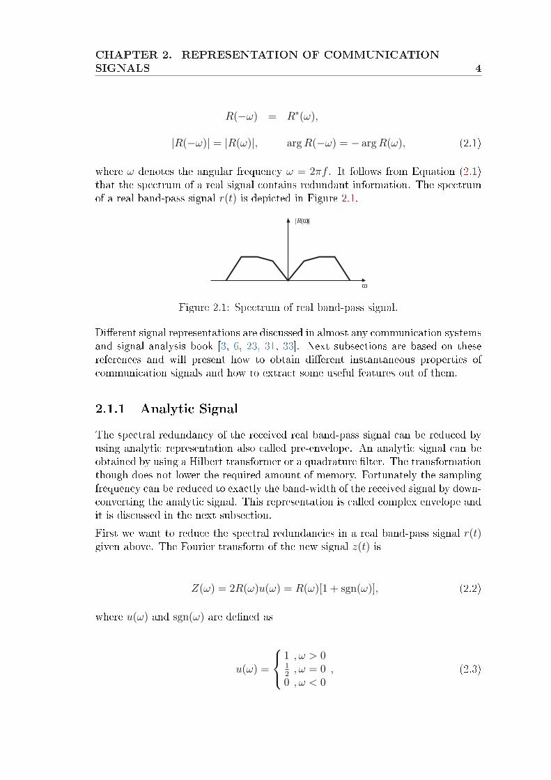
transform pairs are sin x ↔ − cos x and cos x ↔ sin x.Equations (2.2) and (2.5) lead to the analytic signal of the band-pass signal, z(t) =r(t)+jr(t). The digital processing of the analytic signal requires half the samplingrate required for the real signal because the analytic signal has information only inthe right half of the spectrum. Yet it requires the same amount of memory becausethe analytic signal is complex. Spectra of sampled r(t) and z(t) are illustrated inFigure 2.3. Fs denotes the sampling frequency and the solid line represents regionunder half of the sampling frequency.
|R(ω)|
Fs Fs ω
| (ω)|
ωFsFs
Z
Figure 2.3: Spectra of sampled r(t) and z(t).
CHAPTER 2. REPRESENTATION OF COMMUNICATIONSIGNALS 6
2.1.2 Complex EnvelopeThe sampling frequency can be decreased exactly to the band-width of the band-pass signal by using the complex envelope representation. The complex envelopec(t) is obtained from the analytic signal z(t) as follows
c(t) = z(t)e−jωct = m(t) + jn(t), (2.6)
where
m(t) = r(t) cos(ωct) + r(t) sin(ωct),
n(t) = r(t) cos(ωct)− r(t) sin(ωct). (2.7)
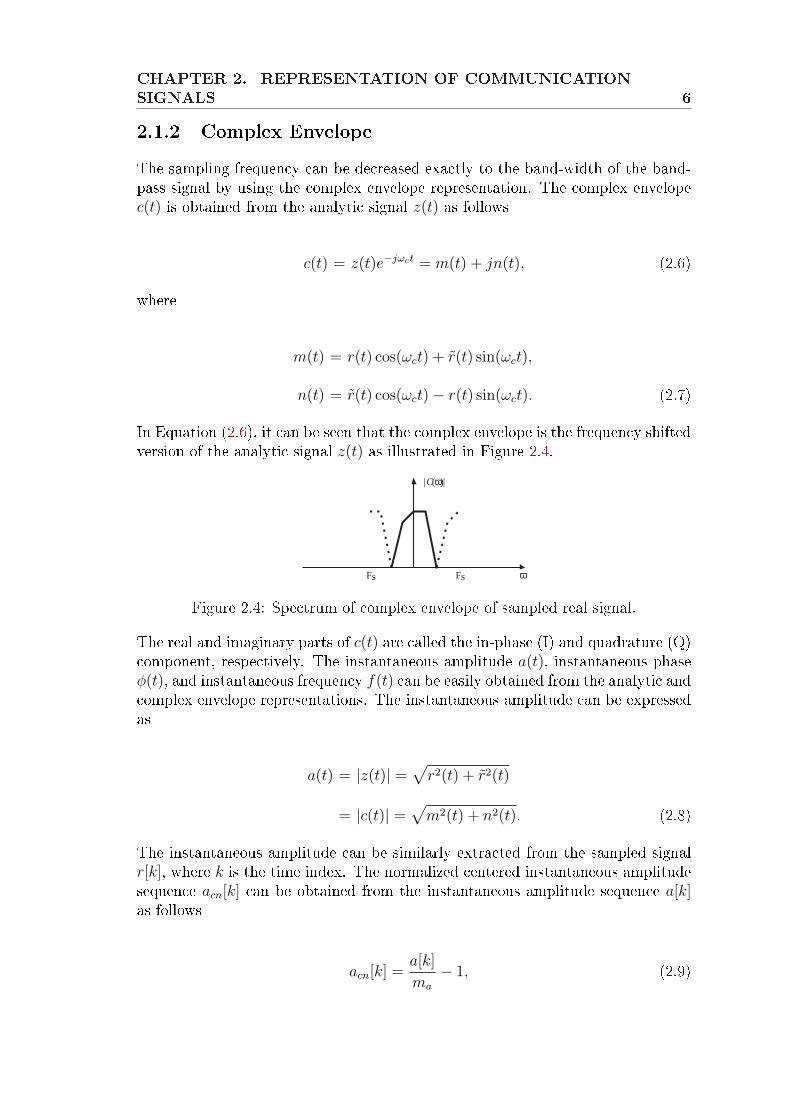
In Equation (2.6), it can be seen that the complex envelope is the frequency shiftedversion of the analytic signal z(t) as illustrated in Figure 2.4.
| (ω)|
ωFsFs
C
Figure 2.4: Spectrum of complex envelope of sampled real signal.
The real and imaginary parts of c(t) are called the in-phase (I) and quadrature (Q)component, respectively. The instantaneous amplitude a(t), instantaneous phaseφ(t), and instantaneous frequency f(t) can be easily obtained from the analytic andcomplex envelope representations. The instantaneous amplitude can be expressedas
a(t) = |z(t)| =√
r2(t) + r2(t)
= |c(t)| =√
m2(t) + n2(t). (2.8)
The instantaneous amplitude can be similarly extracted from the sampled signalr[k], where k is the time index. The normalized centered instantaneous amplitudesequence acn[k] can be obtained from the instantaneous amplitude sequence a[k]as follows
acn[k] =a[k]
ma
− 1, (2.9)
CHAPTER 2. REPRESENTATION OF COMMUNICATIONSIGNALS 7
where
ma =1
Ns
Ns∑
k=1
a[k], (2.10)
and Ns is the number of samples in a segment. Normalization by ma is used tocompensate the channel gain.The instantaneous phase of the signal can be expressed as
φ(t) =
arg z(t)arg c(t) + ωct
. (2.11)
The instantaneous phase of the modulated signal comprises of the linear componentcontributed by the carrier frequency and the nonlinear component contributed bythe modulating signal. In complex envelope representation, the linear phase com-ponent is not present due to the down-conversion. Otherwise the linear componentof the instantaneous phase must be removed in order to obtain the important fea-tures of the modulated signal. If the carrier frequency fc is accurately known, thenonlinear phase component of the sampled signal r[k] can be estimated as follows
φNL[k] = φuw[k]− 2πfck
fs
, (2.12)
where φuw[k] is the unwrapped phase sequence. If the carrier frequency is unknownit can be obtained by linear trend removal using least squares (LS) estimationwhere [3] the sum of squares,
ε =Ns∑
k=1
[φuw[k]− C1k − C2
]2, (2.13)
is minimized. C1 and C2 are the parameters of a linear model. The linear modelcan be represented as φuw = Hc+v, where v is assumed to be the noise contributedby the nonlinear component and the other parameters are
H =
0 11 1... ...
(Ns − 1) 1
, φuw =
φuw(1)φuw(2)
...φuw(Ns)
, c =
[C1
C2
]. (2.14)
CHAPTER 2. REPRESENTATION OF COMMUNICATIONSIGNALS 8
The columns of the matrix H are independent and H has a full rank. The leastsquares estimate can be expressed in matrix form as [37]
c = [HT H]−1HT φuw. (2.15)
The LS estimate gives the maximum likelihood (ML) estimate if the nonlinearcomponent is Gaussian, which is not always the case. The derivative of the in-stantaneous phase is the angular frequency ω(t). The instantaneous frequency ofthe modulated signal can be expressed as
f(t) =1
2πω(t) =
1
2π
dφ(t)
dt, (2.16)
where ω(t) = 2πf(t). The numerical derivative can be obtained from the un-wrapped phase sequence as follows
f [k] = Fsφuw[k + 1]− φuw[k]
2π, (2.17)
where Fs is the sampling frequency. The normalized centered instantaneous fre-quency for a digital modulated signal can be expressed as
fN [k] =f [k]−mf
rs
, (2.18)
where
mf =1
Ns
Ns∑
k=1
f [k], (2.19)
and rs is the symbol rate.
2.2 Analog ModulationAnalog modulation types can be further divided into two groups [6]: linear andexponential modulation or angle modulation. The properties of these groups aregiven in Table 2.1, where W refers to the band-width and X(ω) refers to thespectrum of the modulating signal. Signal-to-noise ratio (SNR) can be increased in
CHAPTER 2. REPRESENTATION OF COMMUNICATIONSIGNALS 9
Table 2.1: Properties of linear and exponential modulationLinear Exponential
Methods AM, DSB, SSB, VSB FM, PMEnvelope Depends on modulating signal ConstantSpectrum Frequency shifted X(ω) Complex ratio to X(ω)Band-width ≤ 2W > 2W
SNR Depends on transmitting power Depends on band-width
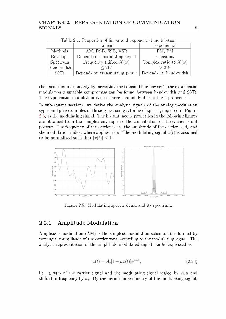
the linear modulation only by increasing the transmitting power; in the exponentialmodulation a suitable compromise can be found between band-width and SNR.The exponential modulation is used more commonly due to these properties.In subsequent sections, we derive the analytic signals of the analog modulationtypes and give examples of these types using a frame of speech, depicted in Figure2.5, as the modulating signal. The instantaneous properties in the following guresare obtained from the complex envelope, so the contribution of the carrier is notpresent. The frequency of the carrier is ωc, the amplitude of the carrier is Ac andthe modulation index, where applies, is µ. The modulating signal x(t) is assumedto be normalized such that |x(t)| ≤ 1.
0 20 40 60 80 100 120 140 160 180 200−1
−0.8
−0.6
−0.4
−0.2
0
0.2
0.4
0.6
0.8
1
Time / ms
Mod
ulat
ing
sign
al
−8000 −6000 −4000 −2000 0 2000 4000 6000 80000
0.1
0.2
0.3
0.4
0.5
0.6
0.7
0.8
0.9
1Spectrum of the modulating signal
Frequency / Hz
Nor
mal
ized
am
plitu
de
Figure 2.5: Modulating speech signal and its spectrum.
2.2.1 Amplitude ModulationAmplitude modulation (AM) is the simplest modulation scheme. It is formed byvarying the amplitude of the carrier wave according to the modulating signal. Theanalytic representation of the amplitude modulated signal can be expressed as
z(t) = Ac[1 + µx(t)]ejωct, (2.20)
i.e. a sum of the carrier signal and the modulating signal scaled by Acµ andshifted in frequency by ωc. By the hermitian symmetry of the modulating signal,
CHAPTER 2. REPRESENTATION OF COMMUNICATIONSIGNALS 10
4.92 4.94 4.96 4.98 5 5.02 5.04 5.06 5.08
x 105
0
0.1
0.2
0.3
0.4
0.5
0.6
0.7
0.8
0.9
1Spectrum of the AM signal
Frequency / HzN
orm
aliz
ed a
mpl
itude
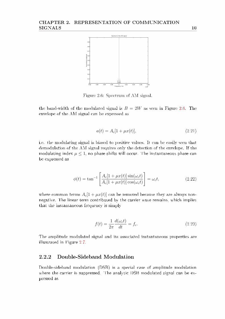
Figure 2.6: Spectrum of AM signal.
the band-width of the modulated signal is B = 2W as seen in Figure 2.6. Theenvelope of the AM signal can be expressed as
a(t) = Ac[1 + µx(t)], (2.21)
i.e. the modulating signal is biased to positive values. It can be easily seen thatdemodulation of the AM signal requires only the detection of the envelope. If themodulating index µ ≤ 1, no phase shifts will occur. The instantaneous phase canbe expressed as
φ(t) = tan−1
[Ac[1 + µx(t)] sin(ωct)
Ac[1 + µx(t)] cos(ωct)
]= ωct, (2.22)
where common terms Ac[1 + µx(t)] can be removed because they are always non-negative. The linear term contributed by the carrier wave remains, which impliesthat the instantaneous frequency is simply
f(t) =1
2π
d(ωct)
dt= fc. (2.23)
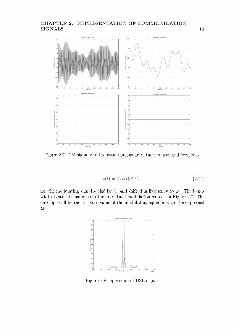
The amplitude modulated signal and its associated instantaneous properties areillustrated in Figure 2.7.
2.2.2 Double-Sideband ModulationDouble-sideband modulation (DSB) is a special case of amplitude modulationwhere the carrier is suppressed. The analytic DSB modulated signal can be ex-pressed as
CHAPTER 2. REPRESENTATION OF COMMUNICATIONSIGNALS 11
0 20 40 60 80 100 120 140 160 180 200−2.5
−2
−1.5
−1
−0.5
0
0.5
1
1.5
2
2.5Amplitude Modulation
Time / ms
Mod
ulat
ed s
igna
l
0 20 40 60 80 100 120 140 160 180 2000
0.5
1
1.5
2
2.5Amplitude Modulation
Time / ms
Inst
anta
neou
s am
plitu
de
0 20 40 60 80 100 120 140 160 180 200
−3
−2
−1
0
1
2
3
Amplitude Modulation
Time / ms
Inst
anta
neou
s ph
ase
/ rad
0 20 40 60 80 100 120 140 160 180 200−50
−40
−30
−20
−10
0
10
20
30
40
50Amplitude Modulation
Time / ms
Inst
anta
neou
s fr
eque
ncy
/ kH
z
Figure 2.7: AM signal and its instantaneous amplitude, phase, and frequency.
z(t) = Acx(t)ejωct, (2.24)
i.e. the modulating signal scaled by Ac and shifted in frequency by ωc. The band-width is still the same as in the amplitude modulation as seen in Figure 2.8. Theenvelope will be the absolute value of the modulating signal and can be expressedas
4.92 4.94 4.96 4.98 5 5.02 5.04 5.06 5.08
x 105
0
0.1
0.2
0.3
0.4
0.5
0.6
0.7
0.8
0.9
1Spectrum of the DSB signal
Frequency / Hz
Nor
mal
ized
am
plitu
de
Figure 2.8: Spectrum of DSB signal.
CHAPTER 2. REPRESENTATION OF COMMUNICATIONSIGNALS 12
a(t) = Ac|x(t)|. (2.25)
Demodulation of the DSB modulated signal cannot be carried out by using anenvelope detector anymore. Therefore a down-converter is needed. There will bealso discontinuities in the instantaneous phase caused by the zero-crossings of themodulating signal. Therefore, the instantaneous phase is obtained by
φ(t) = tan−1
[Acx(t) sin(ωct)
Acx(t) cos(ωct)
]=
ωct , x(t) ≥ 0π + ωct , x(t) < 0
= u(− x(t)
)π + ωct, (2.26)
where u(t) is the unit step function. In other words, there will be a phase shiftof π when the modulating signal crosses zero. Common terms Acx(t) cannot beremoved because the phase information would be lost. This may be deduced withtrigonometric identities, sin(x) = − sin(−x) and cos(x) = cos(−x), as follows
−|x(t)| sin(ωct)
−|x(t)| cos(ωct)=
sin(−ωct)
− cos(−ωct)= − tan(−ωct) = tan(π + ωct). (2.27)
The instantaneous frequency is found by using the fact that the derivative of theunit step function is the Dirac's delta function
f(t) = − x(t)
2δ(− x(t)
)+ fc, (2.28)
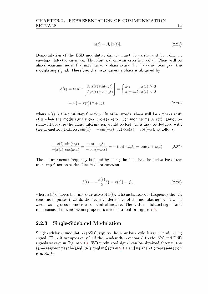
where x(t) denotes the time derivative of x(t). The instantaneous frequency thoughcontains impulses towards the negative derivative of the modulating signal whenzero-crossing occurs and is a constant otherwise. The DSB modulated signal andits associated instantaneous properties are illustrated in Figure 2.9.
2.2.3 Single-Sideband ModulationSingle-sideband modulation (SSB) requires the same band-width as the modulatingsignal. Thus it occupies only half the band-width compared to the AM and DSBsignals as seen in Figure 2.10. SSB modulated signal can be obtained through thesame reasoning as the analytic signal in Section 2.1.1 and its analytic representationis given by
CHAPTER 2. REPRESENTATION OF COMMUNICATIONSIGNALS 13
0 20 40 60 80 100 120 140 160 180 200−1.5
−1
−0.5
0
0.5
1
1.5Double−Sideband Modulation
Time / ms
Mod
ulat
ed s
igna
l
0 20 40 60 80 100 120 140 160 180 2000
0.5
1
1.5Double−Sideband Modulation
Time / ms
Inst
anta
neou
s am
plitu
de
0 20 40 60 80 100 120 140 160 180 200
−3
−2
−1
0
1
2
3
Double−Sideband Modulation
Time / ms
Inst
anta
neou
s ph
ase
/ rad
0 20 40 60 80 100 120 140 160 180 200−50
−40
−30
−20
−10
0
10
20
30
40
50Double−Sideband Modulation
Time / ms
Inst
anta
neou
s fr
eque
ncy
/ kH
z
Figure 2.9: DSB signal and its instantaneous amplitude, phase, and frequency.
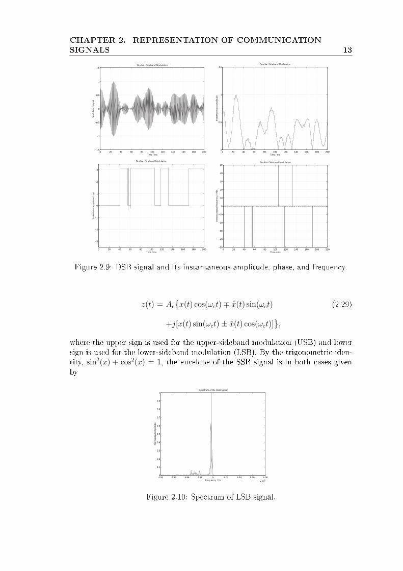
z(t) = Ac
x(t) cos(ωct)∓ x(t) sin(ωct) (2.29)
+j[x(t) sin(ωct)± x(t) cos(ωct)],
where the upper sign is used for the upper-sideband modulation (USB) and lowersign is used for the lower-sideband modulation (LSB). By the trigonometric iden-tity, sin2(x) + cos2(x) = 1, the envelope of the SSB signal is in both cases givenby
4.92 4.94 4.96 4.98 5 5.02 5.04 5.06 5.08
x 105
0
0.1
0.2
0.3
0.4
0.5
0.6
0.7
0.8
0.9
1Spectrum of the SSB signal
Frequency / Hz
Nor
mal
ized
am
plitu
de
Figure 2.10: Spectrum of LSB signal.
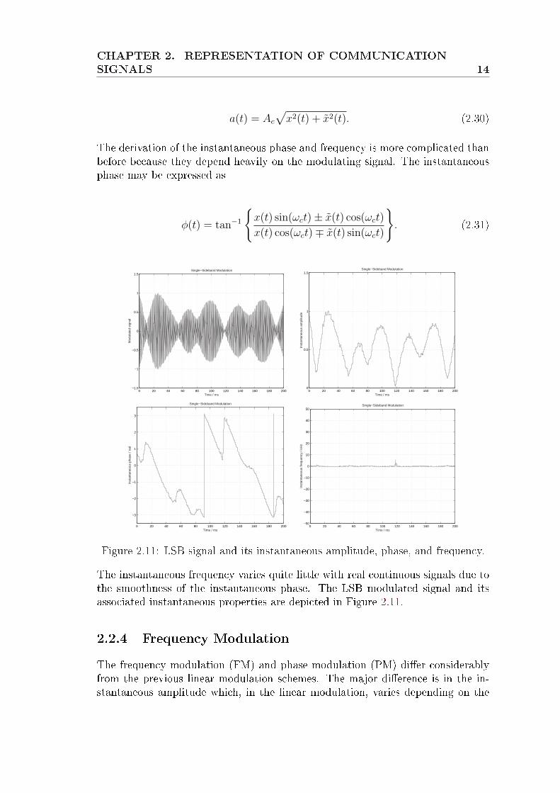
CHAPTER 2. REPRESENTATION OF COMMUNICATIONSIGNALS 14
a(t) = Ac
√x2(t) + x2(t). (2.30)
The derivation of the instantaneous phase and frequency is more complicated thanbefore because they depend heavily on the modulating signal. The instantaneousphase may be expressed as
φ(t) = tan−1
x(t) sin(ωct)± x(t) cos(ωct)
x(t) cos(ωct)∓ x(t) sin(ωct)
. (2.31)
0 20 40 60 80 100 120 140 160 180 200−1.5
−1
−0.5
0
0.5
1
1.5Single−Sideband Modulation
Time / ms
Mod
ulat
ed s
igna
l
0 20 40 60 80 100 120 140 160 180 2000
0.5
1
1.5Single−Sideband Modulation
Time / ms
Inst
anta
neou
s am
plitu
de
0 20 40 60 80 100 120 140 160 180 200
−3
−2
−1
0
1
2
3
Single−Sideband Modulation
Time / ms
Inst
anta
neou
s ph
ase
/ rad
0 20 40 60 80 100 120 140 160 180 200−50
−40
−30
−20
−10
0
10
20
30
40
50Single−Sideband Modulation
Time / ms
Inst
anta
neou
s fr
eque
ncy
/ kH
z
Figure 2.11: LSB signal and its instantaneous amplitude, phase, and frequency.
The instantaneous frequency varies quite little with real continuous signals due tothe smoothness of the instantaneous phase. The LSB modulated signal and itsassociated instantaneous properties are depicted in Figure 2.11.
2.2.4 Frequency ModulationThe frequency modulation (FM) and phase modulation (PM) dier considerablyfrom the previous linear modulation schemes. The major dierence is in the in-stantaneous amplitude which, in the linear modulation, varies depending on the
CHAPTER 2. REPRESENTATION OF COMMUNICATIONSIGNALS 15
modulating signal and, in the exponential modulation, is a constant. In the expo-nential modulation, the angle of the carrier is altered with respect to the modu-lating signal. Thus exponential modulation is often called angle modulation.
4.5 4.6 4.7 4.8 4.9 5 5.1 5.2 5.3 5.4 5.5
x 105
0
0.1
0.2
0.3
0.4
0.5
0.6
0.7
0.8
0.9
1Spectrum of the FM signal
Frequency / Hz
Nor
mal
ized
am
plitu
de
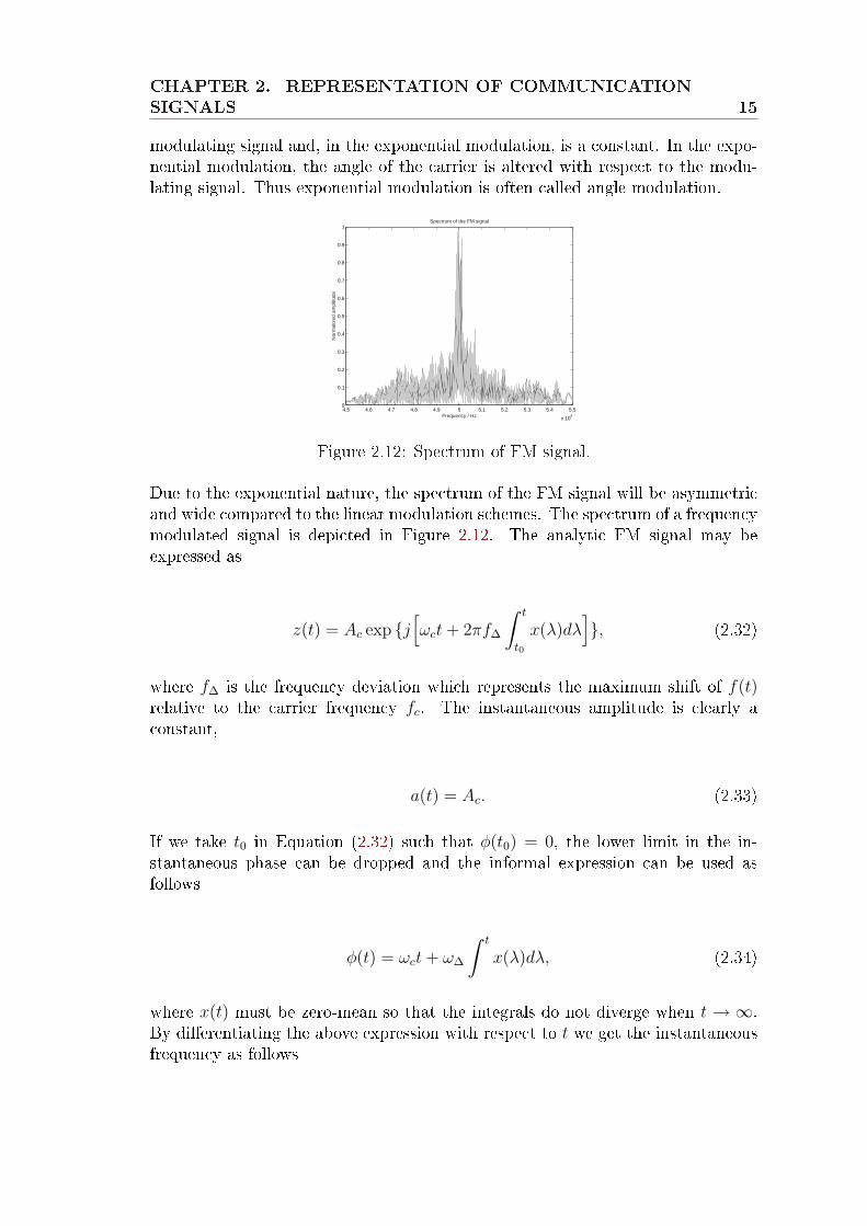
Figure 2.12: Spectrum of FM signal.
Due to the exponential nature, the spectrum of the FM signal will be asymmetricand wide compared to the linear modulation schemes. The spectrum of a frequencymodulated signal is depicted in Figure 2.12. The analytic FM signal may beexpressed as
z(t) = Ac exp j[ωct + 2πf∆
∫ t
t0
x(λ)dλ], (2.32)
where f∆ is the frequency deviation which represents the maximum shift of f(t)relative to the carrier frequency fc. The instantaneous amplitude is clearly aconstant,
a(t) = Ac. (2.33)
If we take t0 in Equation (2.32) such that φ(t0) = 0, the lower limit in the in-stantaneous phase can be dropped and the informal expression can be used asfollows
φ(t) = ωct + ω∆
∫ t
x(λ)dλ, (2.34)
where x(t) must be zero-mean so that the integrals do not diverge when t → ∞.By dierentiating the above expression with respect to t we get the instantaneousfrequency as follows
CHAPTER 2. REPRESENTATION OF COMMUNICATIONSIGNALS 16
0 20 40 60 80 100 120 140 160 180 200−1.5
−1
−0.5
0
0.5
1
1.5Frequency Modulation
Time / ms
Mod
ulat
ed s
igna
l
0 20 40 60 80 100 120 140 160 180 2000
0.5
1
1.5Frequency Modulation
Time / ms
Inst
anta
neou
s am
plitu
de
0 20 40 60 80 100 120 140 160 180 200
−3
−2
−1
0
1
2
3
Frequency Modulation
Time / ms
Inst
anta
neou
s ph
ase
/ rad
0 20 40 60 80 100 120 140 160 180 200−50
−40
−30
−20
−10
0
10
20
30
40
50Frequency Modulation
Time / ms
Inst
anta
neou
s fr
eque
ncy
/ kH
z
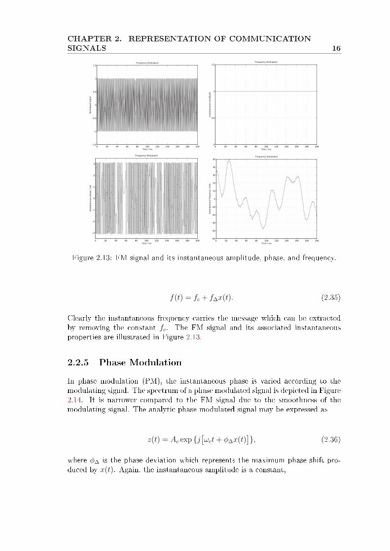
Figure 2.13: FM signal and its instantaneous amplitude, phase, and frequency.
f(t) = fc + f∆x(t). (2.35)
Clearly the instantaneous frequency carries the message which can be extractedby removing the constant fc. The FM signal and its associated instantaneousproperties are illustrated in Figure 2.13.
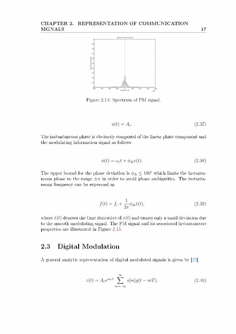
2.2.5 Phase ModulationIn phase modulation (PM), the instantaneous phase is varied according to themodulating signal. The spectrum of a phase modulated signal is depicted in Figure2.14. It is narrower compared to the FM signal due to the smoothness of themodulating signal. The analytic phase modulated signal may be expressed as
z(t) = Ac exp j[ωct + φ∆x(t)], (2.36)
where φ∆ is the phase deviation which represents the maximum phase shift pro-duced by x(t). Again, the instantaneous amplitude is a constant,
CHAPTER 2. REPRESENTATION OF COMMUNICATIONSIGNALS 17
4.92 4.94 4.96 4.98 5 5.02 5.04 5.06 5.08
x 105
0
0.1
0.2
0.3
0.4
0.5
0.6
0.7
0.8
0.9
1Spectrum of the PM signal
Frequency / HzN
orm
aliz
ed a
mpl
itude
Figure 2.14: Spectrum of PM signal.
a(t) = Ac. (2.37)
The instantaneous phase is obviously composed of the linear phase component andthe modulating information signal as follows
φ(t) = ωct + φ∆x(t). (2.38)
The upper bound for the phase deviation is φ∆ ≤ 180 which limits the instanta-neous phase to the range ±π in order to avoid phase ambiguities. The instanta-neous frequency can be expressed as
f(t) = fc +1
2πφ∆x(t), (2.39)
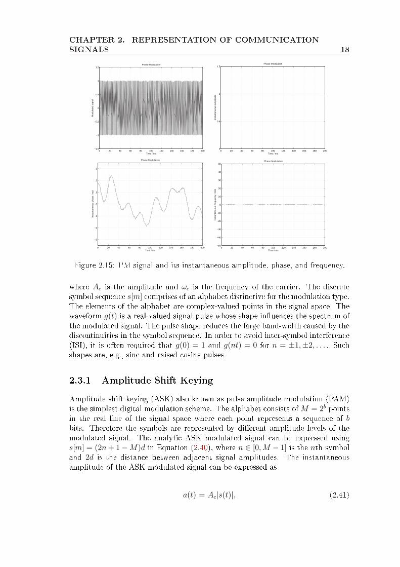
where x(t) denotes the time derivative of x(t) and causes only a small deviation dueto the smooth modulating signal. The PM signal and its associated instantaneousproperties are illustrated in Figure 2.15.
2.3 Digital ModulationA general analytic representation of digital modulated signals is given by [23]
z(t) = Acejωct
∞∑m=−∞
s[m]g(t−mT ), (2.40)
CHAPTER 2. REPRESENTATION OF COMMUNICATIONSIGNALS 18
0 20 40 60 80 100 120 140 160 180 200−1.5
−1
−0.5
0
0.5
1
1.5Phase Modulation
Time / ms
Mod
ulat
ed s
igna
l
0 20 40 60 80 100 120 140 160 180 2000
0.5
1
1.5Phase Modulation
Time / ms
Inst
anta
neou
s am
plitu
de
0 20 40 60 80 100 120 140 160 180 200
−3
−2
−1
0
1
2
3
Phase Modulation
Time / ms
Inst
anta
neou
s ph
ase
/ rad
0 20 40 60 80 100 120 140 160 180 200−50
−40
−30
−20
−10
0
10
20
30
40
50Phase Modulation
Time / ms
Inst
anta
neou
s fr
eque
ncy
/ kH
z
Figure 2.15: PM signal and its instantaneous amplitude, phase, and frequency.
where Ac is the amplitude and ωc is the frequency of the carrier. The discretesymbol sequence s[m] comprises of an alphabet distinctive for the modulation type.The elements of the alphabet are complex-valued points in the signal space. Thewaveform g(t) is a real-valued signal pulse whose shape inuences the spectrum ofthe modulated signal. The pulse shape reduces the large band-width caused by thediscontinuities in the symbol sequence. In order to avoid inter-symbol interference(ISI), it is often required that g(0) = 1 and g(nt) = 0 for n = ±1,±2, . . . . Suchshapes are, e.g., sinc and raised cosine pulses.
2.3.1 Amplitude Shift KeyingAmplitude shift keying (ASK) also known as pulse amplitude modulation (PAM)is the simplest digital modulation scheme. The alphabet consists of M = 2b pointsin the real line of the signal space where each point represents a sequence of bbits. Therefore the symbols are represented by dierent amplitude levels of themodulated signal. The analytic ASK modulated signal can be expressed usings[m] = (2n + 1−M)d in Equation (2.40), where n ∈ [0,M − 1] is the nth symboland 2d is the distance between adjacent signal amplitudes. The instantaneousamplitude of the ASK modulated signal can be expressed as
a(t) = Ac|s(t)|, (2.41)
CHAPTER 2. REPRESENTATION OF COMMUNICATIONSIGNALS 19
where
s(t) =∞∑
m=−∞s[m]g(t−mT ), (2.42)
i.e., the absolute value of the symbol function s(t) with dierent amplitude levelsscaled by Ac. The instantaneous phase is obtained similarly to DSB in analogmodulation because the negative symbol values lead to phase shifts as follows
φ(t) = u(− s(t)
)π + ωct, (2.43)
where u(t) is the unit step function. The instantaneous frequency may be expressedas
f(t) = − s(t)
2δ(− s(t)
)+ fc, (2.44)
0 200 400 600 800 1000 1200 1400 1600 1800 2000−1.5
−1
−0.5
0
0.5
1
1.52ASK/2PSK
Mod
ulat
ed s
igna
l
Time / us0 200 400 600 800 1000 1200 1400 1600 1800 2000
0
0.5
1
1.52ASK/2PSK
Inst
anta
neou
s am
plitu
de
Time / us
0 200 400 600 800 1000 1200 1400 1600 1800 2000−2
−1
0
1
2
3
4
52ASK/2PSK
Inst
anta
neou
s ph
ase
/ rad
Time / us0 200 400 600 800 1000 1200 1400 1600 1800 2000
−1500
−1000
−500
0
500
1000
15002ASK/2PSK
Inst
anta
neou
s fr
eque
ncy
/ kH
z
Time / us
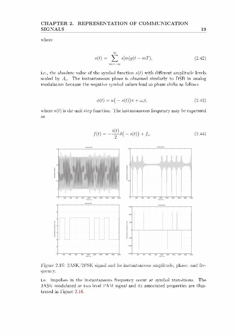
Figure 2.16: 2ASK/2PSK signal and its instantaneous amplitude, phase, and fre-quency.
i.e. impulses in the instantaneous frequency occur at symbol transitions. The2ASK modulated or two level PAM signal and its associated properties are illus-trated in Figure 2.16.
CHAPTER 2. REPRESENTATION OF COMMUNICATIONSIGNALS 20
2.3.2 Phase Shift KeyingPhase shift keying (PSK) is obtained by dening a unique phase state of the carrierfor every symbol as follows
s[m] = ejφ[m], φ[m] ∈ 0, 2π
M, . . . ,
(M − 1)2π
M, (2.45)
where symbols do not have any eect in the instantaneous amplitude. The analyticPSK modulated signal may be expressed as
z(t) = Ac
∞∑m=−∞
ej(ωct+φ[m])g(t−mT ). (2.46)
Usual choices for M are 2, 4 and 8. 2PSK and 4PSK are commonly called binaryphase shift keying (BPSK) and quadrature phase shift keying (QPSK), respec-tively. Larger constellations are too dense and therefore not robust to noise. Thereis still some contribution of g(t) to the envelope but due to the properties of g(t)its sum will be approximately unity. The instantaneous amplitude is given by
a(t) = Ac
∞∑m=−∞
g(t−mT ). (2.47)
The instantaneous phase depends on the summation term m in Equation (2.46).Therefore the expression for the instantaneous phase is
φ(t) = ωct +∞∑
m=−∞φ[m]
[u(t− m− 1
2T
)− u
(t− m + 1
2T
)], (2.48)
where the unit step functions pick up the correct phase term in every time instant.The phase of the modulated signal consists of the phase states caused by thesymbol sequence. The instantaneous frequency is obtained by
f(t) = fc +1
2π
∞∑m=−∞
φ[m][δ(t− m− 1
2T
)− δ
(t− m + 1
2T
)], (2.49)
i.e. again impulses occur at symbol transitions. The 2PSK modulated signal andassociated instantaneous properties are illustrated in Figure 2.16.
CHAPTER 2. REPRESENTATION OF COMMUNICATIONSIGNALS 21
−4 −3 −2 −1 0 1 2 3 4−4
−3
−2
−1
0
1
2
3
416QAM constellation
Imag
inar
yReal
Figure 2.17: Constellation of 16QAM.
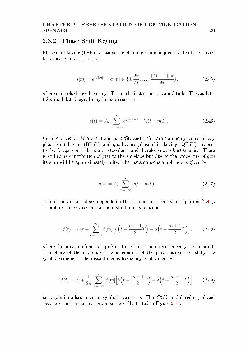
2.3.3 Quadrature Amplitude ModulationQuadrature amplitude modulation (QAM) is a combination of ASK and PSK.The symbols are separated by both amplitude and phase dierences. Often theconstellation is chosen to be square such as 16QAM constellation in Figure 2.17.QAM is mostly used in wired channels, e.g. cables, due to the larger number ofthe symbols and weaker tolerance for noise. Constellations are often chosen to bepowers of two up to M = 256 or more.The symbols may be represented as complex numbers Res[m]+jIms[m], whereRe· denotes the real component and Im· denotes the imaginary component.For the extraction of the instantaneous properties, though, it is more convenientto express the symbols in polar coordinates as follows
s[m] = A[m]ejφ[m], (2.50)
where
A[m] = |s[m]|, and φ[m] = arg s[m]. (2.51)
The analytic QAM signal is now given by
z(t) = Ac
∞∑m=−∞
A[m]ej(ωct+φ[m])g(t−mT ), (2.52)
where A[m] and g(t) are the only terms aecting on the envelope and A[m] ≥ 0, sothe absolute value can be omitted. The instantaneous amplitude may be expressedas
CHAPTER 2. REPRESENTATION OF COMMUNICATIONSIGNALS 22
a(t) = Ac
∞∑m=−∞
A[m]g(t−mT ). (2.53)
Again, because A[m] ≥ 0, it does not have any eect on the instantaneous phase.The instantaneous phase is obtained by
φ(t) = ωct +∞∑
m=−∞φ[m]
[u(t− m− 1
2T
)− u
(t− m + 1
2T
)]. (2.54)
Due to discontinuities in the instantaneous phase the expression for the instanta-neous frequency may be written as
f(t) = fc +1
2π
∞∑m=−∞
φ[m][δ(t− m− 1
2T
)− δ
(t− m + 1
2T
)]. (2.55)
0 200 400 600 800 1000 1200 1400 1600 1800 2000−6
−4
−2
0
2
4
616QAM
Mod
ulat
ed s
igna
l
Time / us0 200 400 600 800 1000 1200 1400 1600 1800 2000
0
1
2
3
4
5
616QAM
Inst
anta
neou
s am
plitu
de
Time / us
0 200 400 600 800 1000 1200 1400 1600 1800 2000
−3
−2
−1
0
1
2
3
16QAM
Inst
anta
neou
s ph
ase
/ rad
Time / us0 200 400 600 800 1000 1200 1400 1600 1800 2000
−200
−150
−100
−50
0
50
10016QAM
Inst
anta
neou
s fr
eque
ncy
/ kH
z
Time / us
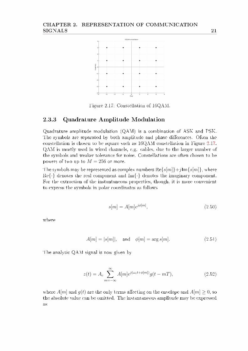
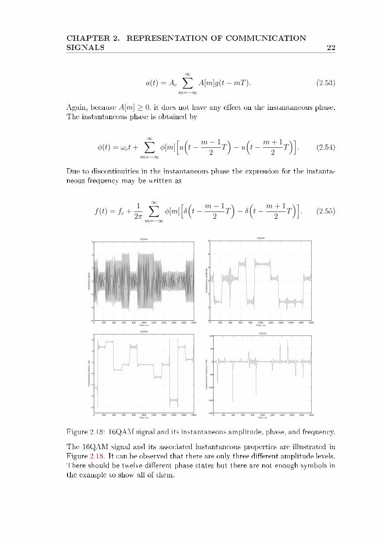
Figure 2.18: 16QAM signal and its instantaneous amplitude, phase, and frequency.
The 16QAM signal and its associated instantaneous properties are illustrated inFigure 2.18. It can be observed that there are only three dierent amplitude levels.There should be twelve dierent phase states but there are not enough symbols inthe example to show all of them.
CHAPTER 2. REPRESENTATION OF COMMUNICATIONSIGNALS 23
2.3.4 Frequency Shift KeyingFrequency shift keying (FSK) diers from the digital modulation schemes describedso far due to the fact that it cannot be represented by Equation (2.40). Theanalysis of FSK will be a combination of methods given earlier and those used forthe FM modulated signals in Section 2.2. The FSK modulated signal comprises ofpulses having dierent frequencies depending on the symbol. Usual choices for thenumber of the dierent frequencies are 2, 4 and 8. The phase of the FSK signalcan be continuous or discontinuous depending on the duration of the pulses. Ifthere is an integer number of periods in every pulse, the phase of the signal willbe continuous. The analytic FSK modulated signal may be expressed as follows
z(t) = Ac exp j[ωct + ω∆
∫ t
s(τ)dτ], (2.56)
where
s(t) =∞∑
m=−∞s[m]g(t−mT ), (2.57)
and ω∆ is the frequency dierence of two adjacent pulses. The signal is calledcontinuous-phase FSK (CPFSK) if the pulse shape g(t − mT ) is a square andf∆ = 1/T . Obviously the envelope of the FSK signal will be a constant
a(t) = Ac. (2.58)
The band-width of the FSK signals may be reduced by choosing f∆ = 1/(2T )which is called minimum shift keying (MSK) and by choosing g(t) as low-passlter with Gaussian shape we get Gaussian MSK (GMSK), which is used in globalsystem for mobiles (GSM). The instantaneous phase is given by
φ(t) = ωct + ω∆
∫ t
s(τ)dτ, (2.59)
where the value of the integral depends only on the pulse shape. The instantaneousfrequency then becomes
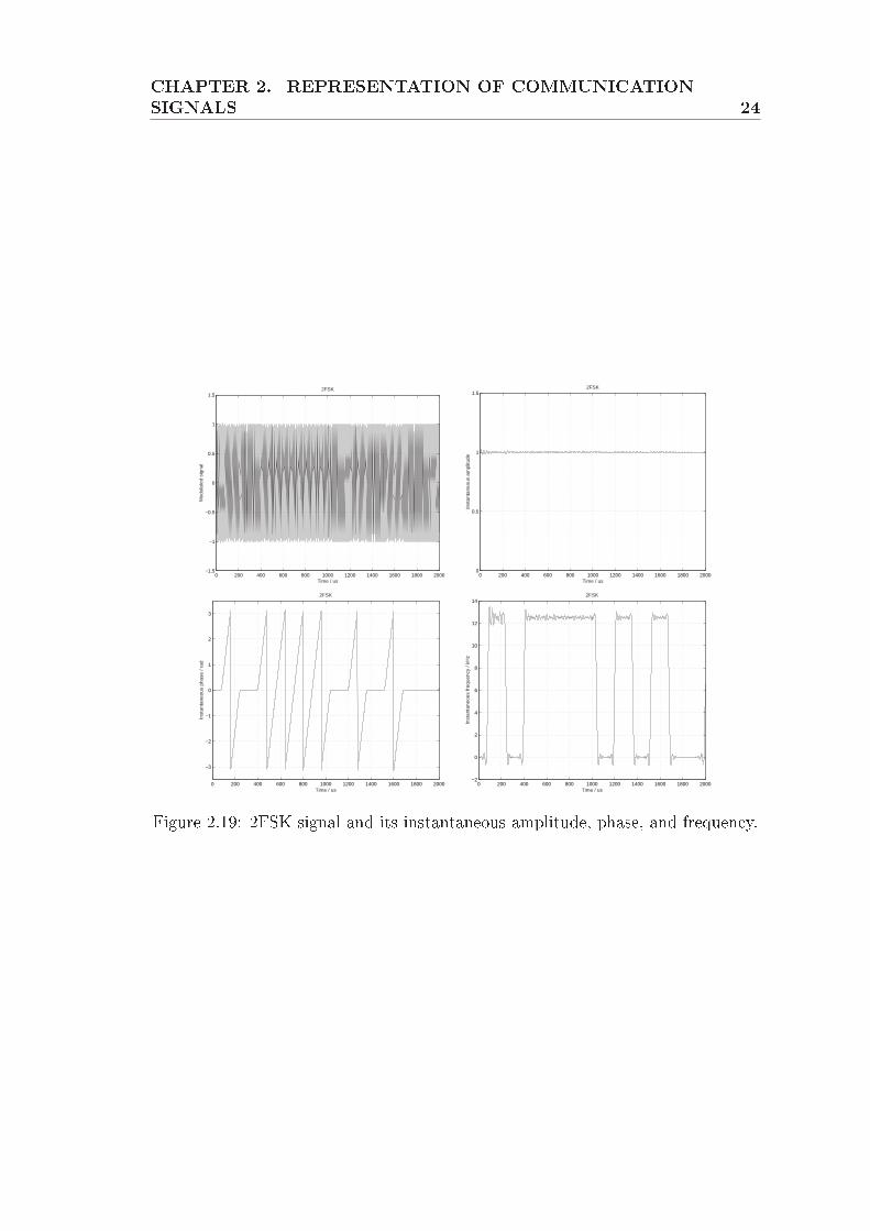
f(t) = fc + f∆s(t), (2.60)
i.e. the instantaneous frequency varies with respect to the symbol values. The2FSK modulated signal and its associated instantaneous properties are illustratedin Figure 2.19. There are also more complicated methods to implement the CPFSKsignals exploiting memory and one or more modulation indices, hk, k ≥ 1. Theseform a general class of continuous-phase modulated (CPM) signals.
CHAPTER 2. REPRESENTATION OF COMMUNICATIONSIGNALS 24
0 200 400 600 800 1000 1200 1400 1600 1800 2000−1.5
−1
−0.5
0
0.5
1
1.52FSK
Mod
ulat
ed s
igna
l
Time / us0 200 400 600 800 1000 1200 1400 1600 1800 2000
0
0.5
1
1.52FSK
Inst
anta
neou
s am
plitu
de
Time / us
0 200 400 600 800 1000 1200 1400 1600 1800 2000
−3
−2
−1
0
1
2
3
2FSK
Inst
anta
neou
s ph
ase
/ rad
Time / us0 200 400 600 800 1000 1200 1400 1600 1800 2000
−2
0
2
4
6
8
10
12
142FSK
Inst
anta
neou
s fr
eque
ncy
/ kH
z
Time / us
Figure 2.19: 2FSK signal and its instantaneous amplitude, phase, and frequency.
Chapter 3
Statistical Tools
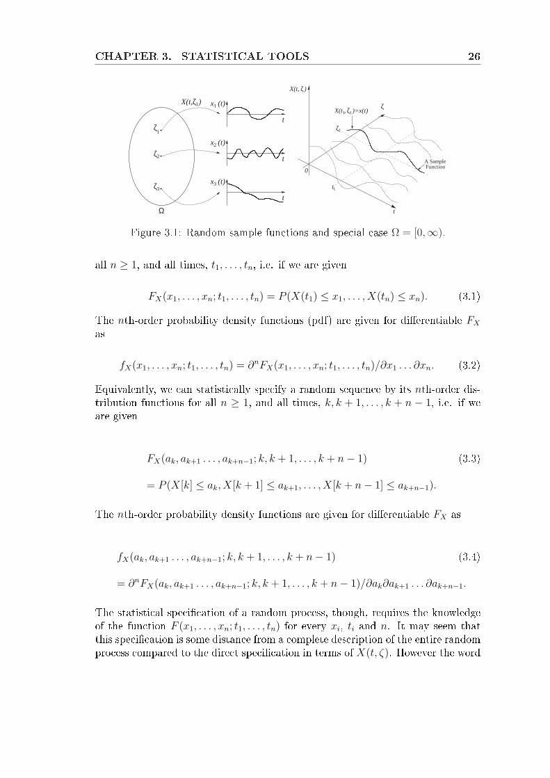
In communication systems, there is a vast amount of uncertainty present in thereceived signal due to unknown modulating signal and unknown modulation type.Hence, it is necessary to consider the received signal as a random process or arandom sequence in the case of a sampled signal. In this chapter we presentstatistics that are useful for the modulation classication task. General denitionsand well-known statistics of the random processes and random sequences may befound in [30, 37], for example.
3.1 Random ProcessesA random process X(t) is a rule for assigning a function X(t, ζ) to every ζ ∈ Ω,where Ω is the sample description space and ζ is an event. Thus, a random processis a family of time-functions depending on the parameter ζ or, equivalently, afunction of t and ζ. The domain of ζ is the set of all experimental outcomesand the domain of t is a set T of real numbers. If T is the real axis, X(t) is acontinuous-time process. If T is the set of integers, then X(t) is a discrete-timeprocess. A discrete-time process is, thus, a sequence of random variables, alsoknown as random sequence. Such a sequence will be denoted by X[k].Three dierent sample functions xi(t), i = 1, 2, 3 are depicted on the left hand sideof Figure 3.1. Each element of the sample description space ζi ∈ Ω maps to acontinuous-time function; i.e. sample function. An example for the special caseΩ = [0,∞) is illustrated on the right hand side of the gure.For a specic t, X(t) is a random variable with distribution FX(x; t) = P (X(t) ≤x). This function depends on t, and it equals the probability of the event X(t) ≤ xconsisting of all outcomes ζi such that, at the specic time t, the samples X(t, ζi)of the given process do not exceed the number x. The function FX(x, t) is calledthe rst-order distribution of the process X(t). The random process is said to bestatistically specied by its nth-order cumulative distribution functions (cdf) for
CHAPTER 3. STATISTICAL TOOLS 26
Ω
1
2
3
t
ζ
ζ
ζ
t
t
ζ1 x (t)1
x (t)2
x (t)3
X(t, )ζ
t
0
t
1
1
A SampleFunction
ζ
ζX(t, )
1 ζ1X(t , )=x(t)
Figure 3.1: Random sample functions and special case Ω = [0,∞).
all n ≥ 1, and all times, t1, . . . , tn, i.e. if we are given
FX(x1, . . . , xn; t1, . . . , tn) = P (X(t1) ≤ x1, . . . , X(tn) ≤ xn). (3.1)
The nth-order probability density functions (pdf) are given for dierentiable FX
as
fX(x1, . . . , xn; t1, . . . , tn) = ∂nFX(x1, . . . , xn; t1, . . . , tn)/∂x1 . . . ∂xn. (3.2)
Equivalently, we can statistically specify a random sequence by its nth-order dis-tribution functions for all n ≥ 1, and all times, k, k + 1, . . . , k + n − 1, i.e. if weare given
FX(ak, ak+1 . . . , ak+n−1; k, k + 1, . . . , k + n− 1) (3.3)
= P (X[k] ≤ ak, X[k + 1] ≤ ak+1, . . . , X[k + n− 1] ≤ ak+n−1).
The nth-order probability density functions are given for dierentiable FX as
fX(ak, ak+1 . . . , ak+n−1; k, k + 1, . . . , k + n− 1) (3.4)
= ∂nFX(ak, ak+1 . . . , ak+n−1; k, k + 1, . . . , k + n− 1)/∂ak∂ak+1 . . . ∂ak+n−1.
The statistical specication of a random process, though, requires the knowledgeof the function F (x1, . . . , xn; t1, . . . , tn) for every xi, ti and n. It may seem thatthis specication is some distance from a complete description of the entire randomprocess compared to the direct specication in terms of X(t, ζ). However the word
CHAPTER 3. STATISTICAL TOOLS 27
statistical indicates that the former information can be obtained, at least concep-tually, by estimating the nth-order cdf's for n = 1, 2, 3, . . . by using statistics. Therst moment or mean function of a random process is
µX(t) , E[X(t)] =
∫ ∞
−∞xf(x; t)dx, −∞ < t < ∞. (3.5)
Similarly the second moment or correlation function is dened as the expectedvalue of the conjugate-product,
RX(t1, t2) , E[X(t1)X∗(t2)] =
∫ ∞
−∞
∫ ∞
−∞x1x
∗2f(x1, x2; t1, t2)dx1dx2,
−∞ < t1, t2 < ∞. (3.6)
The value of RX(t1, t2) on the diagonal t1 = t2 = t is the average power of X(t)because RX(t, t) = E[|X(t)|2]. The second central moment or covariance functionis dened as the expected value of the conjugate-product of the centered process,
CX(t1, t2) , E[(X(t1)− µX(t1))(X(t2)− µX(t2))∗]
= RX(t1, t2)− µX(t1)µ∗X(t2). (3.7)
Also variance function is dened as σ2X(t) , CX(t, t) = E[|X(t)− µX(t)|2].
3.1.1 Stationary ProcessesA random process X(t) is said to be stationary if it has the same nth-order distri-bution function as X(t + T ) for all T and for all positive n. Similarly, a randomsequence X[k] is said to be stationary if for all positive n, the nth-order distri-butions do not depend on the shift parameter τ . This can be expressed by usingdensity functions as
fX(x1, . . . , xn; t1, . . . , tn) = fX(x1, . . . , xn; t1 + T, . . . , tn + T ),
fX(a0, a1 . . . , an−1; τ, τ + 1, . . . , τ + n− 1) = fX(a0, a1 . . . , an−1; 0, 1, . . . , n− 1).(3.8)
By taking T = −t, it follows from above that the rst-order density is fX(x; t) =fX(x, 0) i.e. independent of t and the mean function is µX(t) = µX(0) , µX i.e.a constant. If we choose T = −t2 the second-order density is fX(x1, x2; t1, t2) =
CHAPTER 3. STATISTICAL TOOLS 28
fX(x1, x2; t1 − t2, 0) which depends only on the lag τ = t1 − t2 and the autocorre-lation function can be expressed as RX(t1, t2) = RX(t1− t2, 0) , RX(τ). Similarlyfor the nth-order density T can be chosen in such a way that the density willdepend only on the lags τi, i = 1, . . . , n− 1.A random process is called strict-sense stationary if all its density functions areinvariant to a shift of origin. For most cases strict-sense stationary is too strongan assumption and it is often desirable to partially characterize a random processbased on the knowledge of its rst two moments only, i.e. mean function andautocorrelation function. If the mean function is constant µX(t) , µX for allt and the autocorrelation function is shift-invariant RX(t1 − t2, 0) , RX(τ) forall t1, t2 the random process is said to be wide-sense stationary (WSS). Thus theWSS property is considerably weaker than strict-sense stationarity. We note inparticular that the average power of at least WSS process is also independent of tand equals E[|X(t)|2] = R(0).The power spectral density (PSD) of at least WSS process describes the frequencydistribution of the signal power. The PSD, denoted by S(ω), of a process X(t) isthe Fourier transform of its autocorrelation function R(τ),
S(ω) =
∫ ∞
−∞R(τ)e−jωτdτ, (3.9)
which is the famous Wiener relation. Since R(−τ) = R∗(τ), the PSD of a processX(t) is a real function of ω whether X(t) is real or complex. It means that the PSDdoes not contain any phase information which is a problem in system identication.Stationarity provides the possibility of learning the statistical properties under var-ious ergodicity hypotheses [37]. Generally a statistical description of the randomprocess is not available. Yet for many stationary processes, time-averages will tendto ensemble averages. Such processes are called ergodic.
3.1.2 Cyclostationary ProcessesMany man-made systems such as communication and control systems employ sig-nal formats that have some form of periodic processing operation. Signals pro-duced by samplers, scanners, multiplexors, and modulators are familiar examples.Often these signals are appropriately modeled by random processes that are cy-clostationary (CS), i.e. processes with statistical parameters, such as mean andautocorrelation, that uctuate periodically with time. The processes that havecyclostationary statistics do not have to be periodic in time.The basic books of random processes often give little notice on the cyclostationaryprocesses. Lately the exploitation of the cyclostationary statistics has grown dueto some major benets e.g. in detection and channel identication. Extensivecharacterizations of cyclostationary processes are given by Gardner in [13] andGardner and Franks in [11].
CHAPTER 3. STATISTICAL TOOLS 29
In communications, cyclostationarity often arises due to waveform repetition atthe baud or symbol rate [11]. Therefore oversampling with respect to the symbolrate or several receivers are required. A continuous-time second-order randomprocess X(t); t ∈ (−∞,∞) is dened to be CS in the wide-sense, or of second-order, with cycle period T if and only if its mean and autocorrelation exhibit theperiodicity
µX(t) , E[X(t)] = µX(t + T ),
RX(t1, t2) , E[X(t1)X∗(t2)] = RX(t1 + T, t2 + T ). (3.10)
It is later more convenient to work with the symmetric delay product with τ =t1 − t2. Then the autocorrelation in Equation (3.10) can be rewritten as
RX(t +τ
2, t− τ
2) = E[X(t +
τ
2)X∗(t− τ
2)] = RX(t +
τ
2+ T, t− τ
2+ T ). (3.11)
Since the autocorrelation function is periodic it can be expanded to its Fourierseries representation,
RX(t +τ
2, t− τ
2) =
∑α
RαX(τ)ej2παt, (3.12)
where
RαX(τ) , 1
T
∫ ∞
−∞R(t +
τ
2, t− τ
2)e−j2παtdt, (3.13)
and α is the cyclic frequency. RαX is called cyclic autocorrelation function (CAF)
which is a function of two variables τ and α. For a process that exhibits a singleperiodicity, the range of α is the set of integer multiples, i.e. harmonics of thefundamental frequency. For α = 0 the Fourier series coecient R0
X(τ) is equalto the time averaged probabilistic autocorrelation function RX(τ), dened for aWSS process. Thus, a process X(t) is cyclostationary of second-order if and onlyif Rα
X(τ) 6= 0 for any α 6= 0.If the autocorrelation RX(t + τ
2, t− τ
2) of a process X(t) is not periodic, it cannot
be expanded to a Fourier series. In that case RαX can be dened as [12]
RαX(τ) , 〈X(t +
τ
2)X∗(t− τ
2)e−j2παt〉, (3.14)
CHAPTER 3. STATISTICAL TOOLS 30
where 〈·〉 is the time-averaging operation dened as
〈·〉 , limT→∞
1
T
∫ T/2
−T/2
(·)dt. (3.15)
If RαX(τ) is nonzero for some α 6= 0, the process is called polycyclostationary (or
multiply-cyclostationary or almost cyclostationary).The cyclic autocorrelation function Rα
X can be interpreted as a conventional cross-correlation function of two frequency shifted versions of X(t), namely U(t) ,X(t)e−jπαt and V (t) , X(t)ejπαt. Now the CAF can be expressed as
RUV (τ) , 〈U(t +τ
2)V ∗(t− τ
2)〉 = Rα
X(τ). (3.16)
Similarly to the PSD of stationary process, we can dene the Fourier transform ofthe cyclic autocorrelation for a certain α as
SαX(ω) ,
∫ ∞
−∞Rα
X(τ)e−jωτdτ, (3.17)
which can be considered as a function of two variables ω and α, and it is called thespectral correlation density (SCD) function. There is a similar relation betweenthe SCD at cyclic frequency α = 0 and averaged probabilistic PSD as between theCAF and the averaged probabilistic autocorrelation function.
3.2 Higher-Order StatisticsStatistics can be used to characterize probability density functions and to estimatefX(x) from experimental measurements. The statistics can be determined analyt-ically via the characteristic function of X. The characteristic function is given by[37, 30]
ΦX(ω) , E[ejωX ] =
∫ ∞
−∞fX(x)ejωxdx, (3.18)
which except for a minus sign in the exponent, is the Fourier transform of fX(x).For the Gaussian random variable X with distribution N(µ, σ2) the characteristicfunction can be shown to be
ΦX(ω) = exp(jµω − σ2
2ω2). (3.19)
CHAPTER 3. STATISTICAL TOOLS 31
The inversion of the characteristic function can be obtained similarly to the inverseFourier transform and can be expressed as
fX(x) , 1
2π
∫ ∞
−∞ΦX(ω)e−jωxdω. (3.20)
Due to the inversion formula, knowing ΦX is equivalent to knowing fX(x) and viceversa. By the properties of the Fourier transform the characteristic functions gainone desirable property; i.e. the convolution theorem. Since the pdf fZ(z) of thesum of independent random variables Z = X1 + · · · + XN is the convolution oftheir pdf's fX1(z), . . . , fX2(z), the characteristic function of fZ(z) is the productof the individual functions as follows
fZ(z) = fX1(z) ∗ fX2(z) ∗ · · · ∗ fXN(z),
ΦZ(ω) = ΦX1(ω)ΦX2(ω) . . . ΦXN(ω), (3.21)
where ∗ denotes convolution.
3.2.1 Higher-Order MomentsIf we consider the denition of the characteristic function in Equation (3.18), theexponent function inside the expectation can be expanded to a power series asfollows
ΦX(ω) = E[ejωX ] = E[ ∞∑
n=0
(jωX)n
n!
]=
∞∑n=0
(jω)n
n!mX
n
= 1 +jω
1!mX
1 +(jω)2
2!mX
2 +(jω)3
3!mX
3 + . . . , (3.22)
where mXn is the nth-order moment of X, i.e. mX
n = E[Xn]. Now the nth-ordermoment of X can be obtained by calculating the nth-order derivative of ΦX(ω)with respect to ω at point ω = 0 as follows
mXn =
1
jn
dn
dωnΦX(ω)
∣∣∣ω=0
. (3.23)
This implies that the knowledge of all the moments of X characterizes the pdffX(x) completely. According to Equation (3.19) the Gaussian random variableX has innite number of moments due to the derivation rule of the exponentialfunction.
CHAPTER 3. STATISTICAL TOOLS 32
If X[k] is a real stationary discrete-time signal and its moments up to order nexist, then [28, 29]
mXn (τ1, τ2, . . . , τn−1) , E
[X[k]X[k + τ1] . . . X[k + τn−1]
](3.24)
represents the nth-order moment function of X[k], which depends only on thetime dierences τ1, τ2, . . . , τn−1, τi = 0,±1,±2, . . . for all i. It can be easily seenthat the rst-order moment is the mean of the sequence and the second-ordermoment is the autocorrelation function as follows
µX , mX1 ,
RX(τ) , mX2 (τ1). (3.25)
3.2.2 Cumulants and Multi-CorrelationsIf we take the natural logarithm of the characteristic function, we get the cumu-lative function ΨZ(ω) or the second characteristic function [12, 30]. The benetof the cumulative function comes from the fact that the product in the Equation(3.21) changes to a sum as follows
ΨZ(ω) , ln ΦZ(ω) = ln ΦX1(ω) + ln ΦX2(ω) + · · ·+ ln ΦXN(ω)
= ΨX1(ω) + ΨX2(ω) + · · ·+ ΨXN(ω). (3.26)
Similarly, the nth-order cumulant of a random variable X can be obtained bycalculating the nth-order derivative of the cumulative function at ω = 0 as
cXn =
1
jn
dn
dωnΨX(ω)
∣∣∣ω=0
. (3.27)
The nth-order cumulants of the Gaussian random variable X are identically zerofor n > 2 because the cumulative function for X is a second-order polynomial ofω. From Equation (3.19), it follows that
ΨX(ω) = jµω − σ2
2ω2. (3.28)
The nth-order cumulant of a non-Gaussian stationary random signal, X[k], forn = 3, 4 can be written as [28]
cXn (τ1, τ2, . . . , τn−1) = mX
n (τ1, τ2, . . . , τn−1)−mGn (τ1, τ2, . . . , τn−1), (3.29)
CHAPTER 3. STATISTICAL TOOLS 33
where the rst term mXn (τ1, τ2, . . . , τn−1) is the nth-order moment function of X[k]
and mGn (τ1, τ2, . . . , τn−1) is the nth-order moment function of an equivalent Gaus-
sian signal that has the same mean value and autocorrelation sequence as X[k].Obviously, if X[k] is Gaussian, mX
n (τ1, τ2, . . . , τn−1) = mGn (τ1, τ2, . . . , τn−1) and
thus cXn (τ1, τ2, . . . , τn−1) = 0 for n = 3, 4. For a zero-mean process X[k], the
relationships between the moment and cumulant sequences can [28] be expressedas
cX1 = E
[X[k]
]= mX
1 = 0, (3.30)
cX2 (τ1) = E
[X[k]X[k + τ1]
]= mX
2 (τ1) = mX2 (−τ1) = cX
2 (−τ1), (3.31)
cX3 (τ1, τ2) = E
[X[k]X[k + τ1]X[k + τ2]
]= mX
3 (τ1, τ2), (3.32)
cX4 (τ1, τ2, τ3) = E
[X[k]X[k + τ1]X[k + τ2]X[k + τ3]
]− cX2 (τ1)c
X2 (τ2 − τ3)
−cX2 (τ2)c
X2 (τ3 − τ1)− cX
2 (τ3)cX2 (τ1 − τ2)
= mX4 (τ1, τ2, τ3)−mX
2 (τ1)mX2 (τ3 − τ2)
−mX2 (τ2)m
X2 (τ3 − τ1)−mX
2 (τ3)mX2 (τ2 − τ1). (3.33)
If the signal X[k] is zero-mean, it follows from Equations (3.31) and (3.32) thatthe second and third-order cumulants are identical to the second and third-ordermoments, respectively. Therefore the fourth-order cumulants are important if therandom process is symmetrically distributed.By putting τ1 = τ2 = τ3 = 0 and assuming mX
1 = 0, we obtain very importantresults as follows
γX2 = E
[X2[k]
]= cX
2 (0), (3.34)
γX3 = E
[X3[k]
]= cX
3 (0, 0), (3.35)
γX4 = E
[X4[k]
]− 3(γX2 )2 = cX
4 (0, 0, 0). (3.36)
These values describe the shape of the pdf of X[k]; i.e. γX2 is the variance and
describes the width of the pdf, γX3 is the skewness and describes the symmetry,
and γX4 is the kurtosis and describes the peakedness.
In Figure 3.2, there is a zero-mean Gaussian density with variance σ2X = 0.5
estimated from a random sequence of 200000 samples. Theoretical values of theskewness and kurtosis of the Gaussian pdf can be evaluated from Equation (3.28)
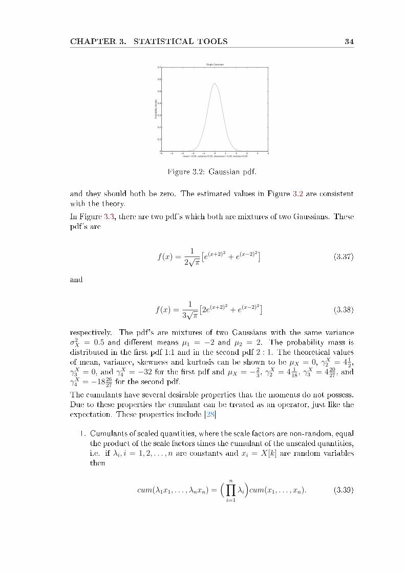
CHAPTER 3. STATISTICAL TOOLS 34
−5 −4 −3 −2 −1 0 1 2 3 4 50
0.1
0.2
0.3
0.4
0.5
0.6
0.7Single Gaussian
Pro
babi
lity
dens
itymean=−0.00, variance=0.50, skewness=−0.00, kurtosis=0.00
Figure 3.2: Gaussian pdf.
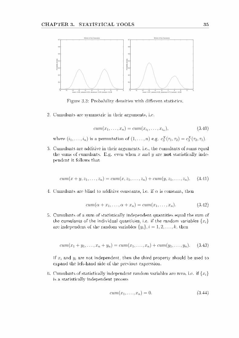
and they should both be zero. The estimated values in Figure 3.2 are consistentwith the theory.In Figure 3.3, there are two pdf's which both are mixtures of two Gaussians. Thesepdf's are
f(x) =1
2√
π
[e(x+2)2 + e(x−2)2
](3.37)
and
f(x) =1
3√
π
[2e(x+2)2 + e(x−2)2
](3.38)
respectively. The pdf's are mixtures of two Gaussians with the same varianceσ2
X = 0.5 and dierent means µ1 = −2 and µ2 = 2. The probability mass isdistributed in the rst pdf 1:1 and in the second pdf 2 : 1. The theoretical valuesof mean, variance, skewness and kurtosis can be shown to be µX = 0, γX
2 = 412,
γX3 = 0, and γX
4 = −32 for the rst pdf and µX = −23, γX
2 = 4 118, γX
3 = 42027, and
γX4 = −1826
27for the second pdf.
The cumulants have several desirable properties that the moments do not possess.Due to these properties the cumulant can be treated as an operator, just like theexpectation. These properties include [28]
1. Cumulants of scaled quantities, where the scale factors are non-random, equalthe product of the scale factors times the cumulant of the unscaled quantities,i.e. if λi, i = 1, 2, . . . , n are constants and xi = X[k] are random variablesthen
cum(λ1x1, . . . , λnxn) =( n∏
i=1
λi
)cum(x1, . . . , xn). (3.39)
CHAPTER 3. STATISTICAL TOOLS 35
−5 −4 −3 −2 −1 0 1 2 3 4 50
0.1
0.2
0.3
0.4
0.5
0.6
0.7Mixture of two Gaussians
Pro
babi
lity
dens
ity
mean=−0.00, variance=4.50, skewness=−0.00, kurtosis=−31.98−5 −4 −3 −2 −1 0 1 2 3 4 50
0.1
0.2
0.3
0.4
0.5
0.6
0.7Mixture of two Gaussians
Pro
babi
lity
dens
ity
mean=−0.67, variance=4.06, skewness=4.73, kurtosis=−18.98
Figure 3.3: Probability densities with dierent statistics.
2. Cumulants are symmetric in their arguments, i.e.
cum(x1, . . . , xn) = cum(xi1 , . . . , xin), (3.40)
where (i1, . . . , in) is a permutation of (1, . . . , n) e.g. cX3 (τ1, τ2) = cX
3 (τ2, τ1).
3. Cumulants are additive in their arguments, i.e., the cumulants of sums equalthe sums of cumulants. E.g. even when x and y are not statistically inde-pendent it follows that
cum(x + y, z1, . . . , zn) = cum(x, z1, . . . , zn) + cum(y, z1, . . . , zn). (3.41)
4. Cumulants are blind to additive constants, i.e. if α is constant, then
cum(α + x1, . . . , α + xn) = cum(x1, . . . , xn). (3.42)
5. Cumulants of a sum of statistically independent quantities equal the sum ofthe cumulants of the individual quantities, i.e. if the random variables xiare independent of the random variables yi, i = 1, 2, . . . , k, then
cum(x1 + y1, . . . , xn + yn) = cum(x1, . . . , xn) + cum(y1, . . . , yn). (3.43)
If xi and yi are not independent, then the third property should be used toexpand the left-hand side of the previous expression.
6. Cumulants of statistically independent random variables are zero, i.e. if xiis a statistically independent process
cum(x1, . . . , xn) = 0. (3.44)
CHAPTER 3. STATISTICAL TOOLS 36
The p + qth-order multi-correlation of a complex-valued stationary random signalis dened [1] as follows
CX,p+q,p(τ1, . . . , τp+q−1) = cum(X(t), X(t + τ1), . . . , X(t + τp−1),
X∗(t− τp), . . . , X∗(t− τp+q−1)
). (3.45)
In this notation p+ q is the order of the multi-correlation whereas p represents thenumber of non-conjugated components. The properties of the multi-correlationare direct consequences of the properties of the cumulants described earlier.
3.2.3 Higher-Order SpectraHigher-order spectra (HOS) are multi-dimensional Fourier transforms of higher-order statistics. They are dened either in terms of cumulants or moments andtheir Fourier transforms are called cumulant spectra or moment spectra respec-tively [28]. Thus, the polyspectra are dened in terms of the cumulants as follows
CXn (ω1, ω2, . . . , ωn−1) =
∞∑τ1=−∞
· · ·∞∑
τn−1=−∞cXn (τ1, τ2, . . . , τn−1) exp
− j
n−1∑i=1
ωiτi
.
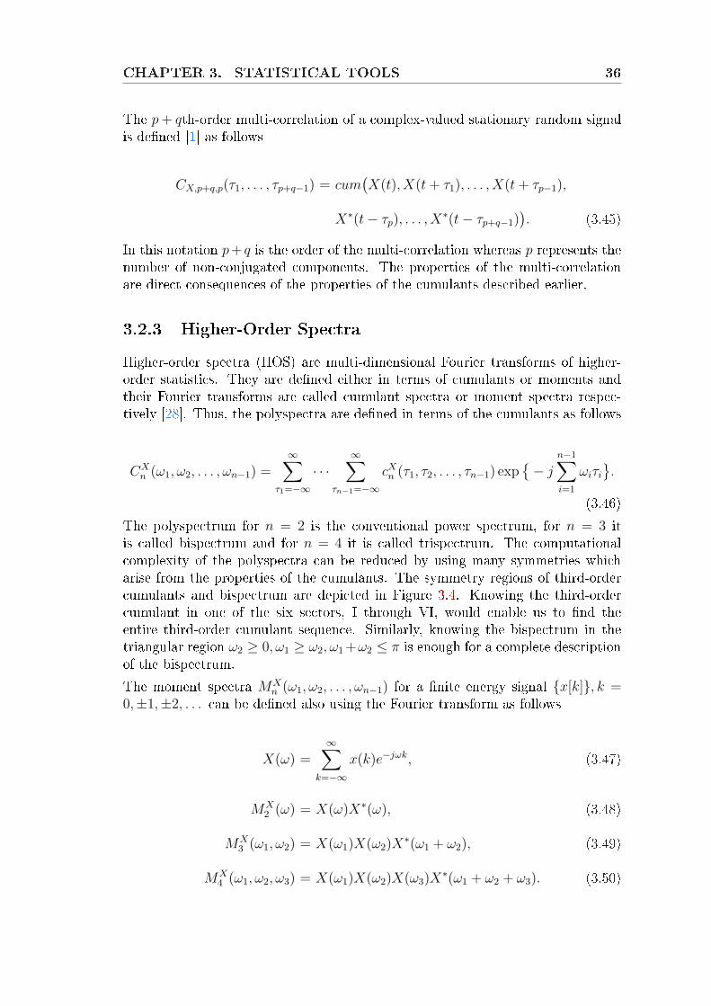
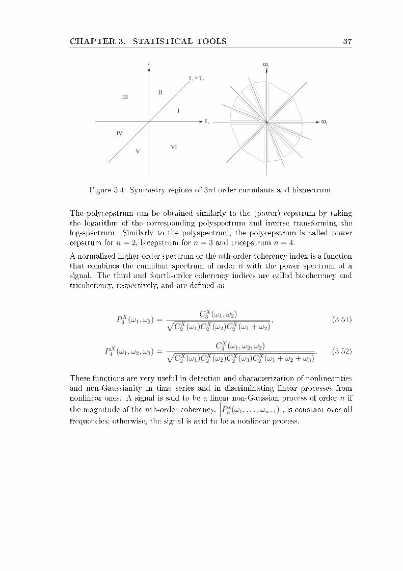
(3.46)The polyspectrum for n = 2 is the conventional power spectrum, for n = 3 itis called bispectrum and for n = 4 it is called trispectrum. The computationalcomplexity of the polyspectra can be reduced by using many symmetries whicharise from the properties of the cumulants. The symmetry regions of third-ordercumulants and bispectrum are depicted in Figure 3.4. Knowing the third-ordercumulant in one of the six sectors, I through VI, would enable us to nd theentire third-order cumulant sequence. Similarly, knowing the bispectrum in thetriangular region ω2 ≥ 0, ω1 ≥ ω2, ω1 +ω2 ≤ π is enough for a complete descriptionof the bispectrum.The moment spectra MX
n (ω1, ω2, . . . , ωn−1) for a nite energy signal x[k], k =0,±1,±2, . . . can be dened also using the Fourier transform as follows
X(ω) =∞∑
k=−∞x(k)e−jωk, (3.47)
MX2 (ω) = X(ω)X∗(ω), (3.48)
MX3 (ω1, ω2) = X(ω1)X(ω2)X
∗(ω1 + ω2), (3.49)
MX4 (ω1, ω2, ω3) = X(ω1)X(ω2)X(ω3)X
∗(ω1 + ω2 + ω3). (3.50)
CHAPTER 3. STATISTICAL TOOLS 37
τ
τ
ττ = 2
1
2
1
II
IV
V
I
III
VI
1
ω
ω
2
Figure 3.4: Symmetry regions of 3rd-order cumulants and bispectrum.
The polycepstrum can be obtained similarly to the (power) cepstrum by takingthe logarithm of the corresponding polyspectrum and inverse transforming thelog-spectrum. Similarly to the polyspectrum, the polycepstrum is called powercepstrum for n = 2, bicepstrum for n = 3 and tricepstrum n = 4.A normalized higher-order spectrum or the nth-order coherency index is a functionthat combines the cumulant spectrum of order n with the power spectrum of asignal. The third and fourth-order coherency indices are called bicoherency andtricoherency, respectively, and are dened as
PX3 (ω1, ω2) =
CX3 (ω1, ω2)√
CX2 (ω1)CX
2 (ω2)CX2 (ω1 + ω2)
, (3.51)
PX4 (ω1, ω2, ω3) =
CX4 (ω1, ω2, ω2)√
CX2 (ω1)CX
2 (ω2)CX2 (ω3)CX
2 (ω1 + ω2 + ω3). (3.52)
These functions are very useful in detection and characterization of nonlinearitiesand non-Gaussianity in time series and in discriminating linear processes fromnonlinear ones. A signal is said to be a linear non-Gaussian process of order n ifthe magnitude of the nth-order coherency,
∣∣∣P xn (ω1, . . . , ωn−1)
∣∣∣, is constant over allfrequencies; otherwise, the signal is said to be a nonlinear process.
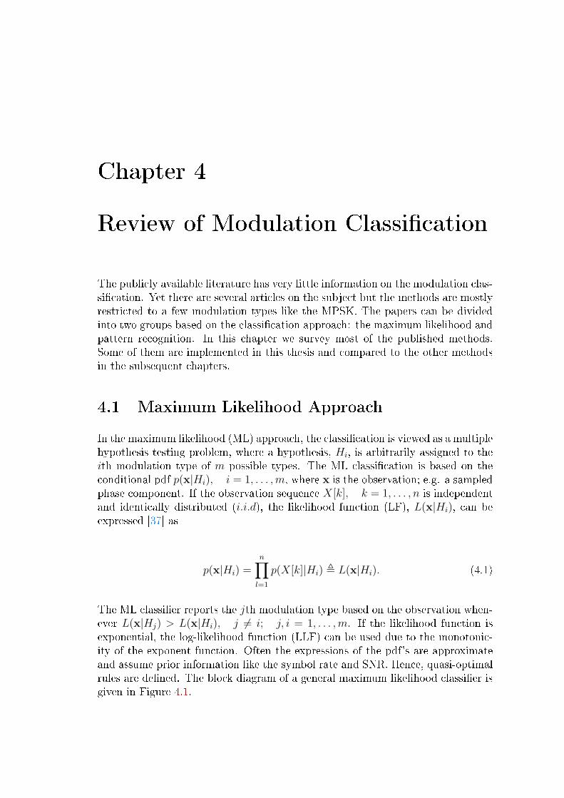
Chapter 4
Review of Modulation Classication
The publicly available literature has very little information on the modulation clas-sication. Yet there are several articles on the subject but the methods are mostlyrestricted to a few modulation types like the MPSK. The papers can be dividedinto two groups based on the classication approach: the maximum likelihood andpattern recognition. In this chapter we survey most of the published methods.Some of them are implemented in this thesis and compared to the other methodsin the subsequent chapters.
4.1 Maximum Likelihood ApproachIn the maximum likelihood (ML) approach, the classication is viewed as a multiplehypothesis testing problem, where a hypothesis, Hi, is arbitrarily assigned to theith modulation type of m possible types. The ML classication is based on theconditional pdf p(x|Hi), i = 1, . . . , m, where x is the observation; e.g. a sampledphase component. If the observation sequence X[k], k = 1, . . . , n is independentand identically distributed (i.i.d), the likelihood function (LF), L(x|Hi), can beexpressed [37] as
p(x|Hi) =n∏
l=1
p(X[k]|Hi) , L(x|Hi). (4.1)
The ML classier reports the jth modulation type based on the observation when-ever L(x|Hj) > L(x|Hi), j 6= i; j, i = 1, . . . , m. If the likelihood function isexponential, the log-likelihood function (LLF) can be used due to the monotonic-ity of the exponent function. Often the expressions of the pdf's are approximateand assume prior information like the symbol rate and SNR. Hence, quasi-optimalrules are dened. The block diagram of a general maximum likelihood classier isgiven in Figure 4.1.
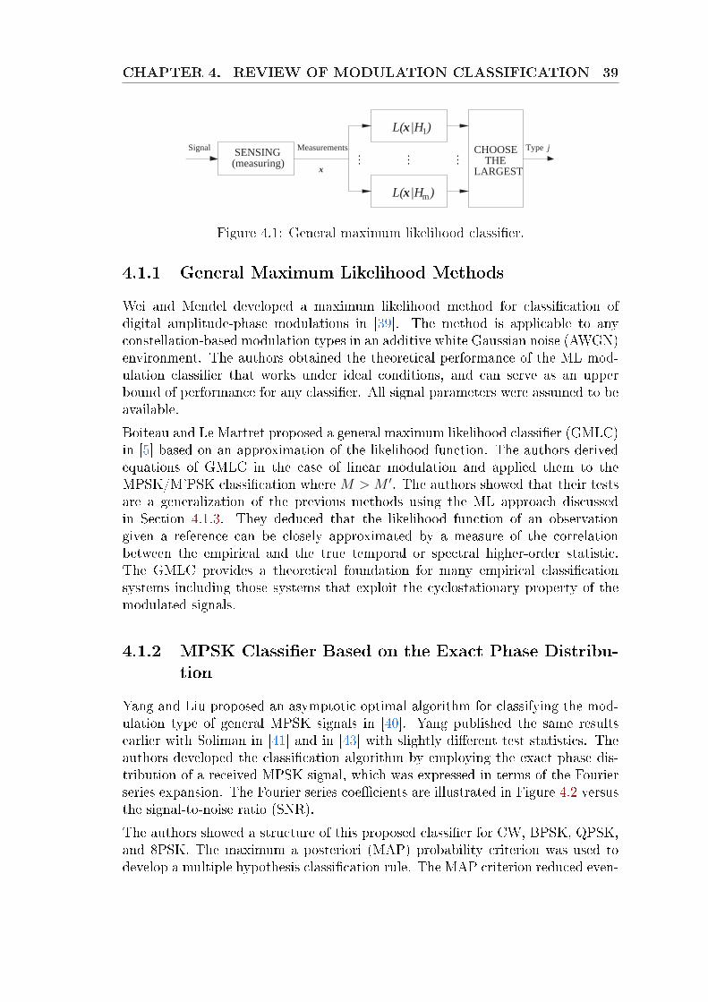
CHAPTER 4. REVIEW OF MODULATION CLASSIFICATION 39
SENSING(measuring)
Signal Measurements
x mL( |H )
L( |H )x 1
LARGESTTHE
CHOOSE Type j
x
Figure 4.1: General maximum likelihood classier.
4.1.1 General Maximum Likelihood MethodsWei and Mendel developed a maximum likelihood method for classication ofdigital amplitude-phase modulations in [39]. The method is applicable to anyconstellation-based modulation types in an additive white Gaussian noise (AWGN)environment. The authors obtained the theoretical performance of the ML mod-ulation classier that works under ideal conditions, and can serve as an upperbound of performance for any classier. All signal parameters were assumed to beavailable.Boiteau and Le Martret proposed a general maximum likelihood classier (GMLC)in [5] based on an approximation of the likelihood function. The authors derivedequations of GMLC in the case of linear modulation and applied them to theMPSK/M'PSK classication where M > M ′. The authors showed that their testsare a generalization of the previous methods using the ML approach discussedin Section 4.1.3. They deduced that the likelihood function of an observationgiven a reference can be closely approximated by a measure of the correlationbetween the empirical and the true temporal or spectral higher-order statistic.The GMLC provides a theoretical foundation for many empirical classicationsystems including those systems that exploit the cyclostationary property of themodulated signals.
4.1.2 MPSK Classier Based on the Exact Phase Distribu-tion
Yang and Liu proposed an asymptotic optimal algorithm for classifying the mod-ulation type of general MPSK signals in [40]. Yang published the same resultsearlier with Soliman in [41] and in [43] with slightly dierent test statistics. Theauthors developed the classication algorithm by employing the exact phase dis-tribution of a received MPSK signal, which was expressed in terms of the Fourierseries expansion. The Fourier series coecients are illustrated in Figure 4.2 versusthe signal-to-noise ratio (SNR).The authors showed a structure of this proposed classier for CW, BPSK, QPSK,and 8PSK. The maximum a posteriori (MAP) probability criterion was used todevelop a multiple hypothesis classication rule. The MAP criterion reduced even-
CHAPTER 4. REVIEW OF MODULATION CLASSIFICATION 40
0 5 10 15 20 2510
−25
10−20
10−15
10−10
10−5
100
m
Coe
ffici
ent v
alue
0 dB−2 dB−5 dB−8 dB−10 dB
Figure 4.2: Coecients cm of the exact phase pdf.
tually to a ML classier because the hypotheses were assumed equally likely. Theperformance of this classier was shown to be more eective than the earlier clas-siers in [41, 43]. The SNR was assumed to be known.
4.1.3 Classiers Based on the Likelihood FunctionsQuasi Log-Likelihood Ratio Classier
Kim and Polydoros proposed a quasi log-likelihood ratio classier (qLLRC) forBPSK and QPSK in [20, 32] and compared it to the more traditional, ad-hoctechniques of the square-law classier (SLC) and the phase-based classier (PBC).The qLLRC was derived by approximating the likelihood functions of the phasemodulated digital signals in white Gaussian noise. The authors showed that itsperformance is signicantly better than that of the intuitively designed PBC, orthe conventional SLC. The capability of the qLLRC algorithm is, though, limitedsince it is only valid for low SNR (SNR< 0dB). All signal parameters such asthe carrier frequency, initial phase, symbol rate and SNR were assumed to beavailable. The classier can only be used to discriminate between the BPSK andQPSK signals.
M th-law Classier versus qM -Rule
Hwang and Polydoros proposed a maximum likelihood classier based on the like-lihood function of MPSK and MQAM signals in additive white Gaussian noise in[19]. The authors derived simplied versions of the LF for each modulation typedenoted by the qM -statistic. The qM -classier can be interpreted as a synchronous,pulse-shape matched-lter. The performance of the qM -rule was compared againstM th-law approaches like [34] reviewed in Section 4.2.2. The correct classicationprobability was approximated in a low SNR (SNR¿ 0dB) with long observationtime, i.e., N À 1 symbols. To achieve the same performance with the M th-law
CHAPTER 4. REVIEW OF MODULATION CLASSIFICATION 41
classier additional gain in the SNR was shown to be more than 2dB. The qM -ruleis only valid for low SNR (SNR< 0dB) and all signal parameters such as the carrierfrequency, initial phase, symbol rate and SNR were assumed to be available.
Average Log-Likelihood Ratio Classier
Long, Chugg and Polydoros extended the low SNR methods to moderate andhigh SNR environments in [24]. The authors presented the Qm-rule based on theaverage log-likelihood ratio (ALLR) and an approximate expression for the pdf ofthe Qm-statistic was developed for medium and high SNR cases. The performanceof the Qm-rule was evaluated in four dierent environments; e.g. in TV andCPFSK interference. The approximation of the ALLR demonstrated an abilityto dramatically improve the performance compared to the qM -rule in [19]. Theclassier was developed for binary hypothesis testing and all signal parameterswere assumed to be available.
Classication in Unknown ISI Environments
Lay and Polydoros developed two classication techniques for digital modulatedsignals aected by an inter-symbol interference (ISI). The initial development ofthe classication tests have been derived assuming a known channel impulse re-sponse. The authors presented an average likelihood ratio test (ALRT) and a gen-eral likelihood ratio test (GLRT) and exploited a per-survivor processing (PSP) forthe channel identication simultaneously. Pairwise classication tests for 16-arydigital modulations in known and unknown channels were simulated. The ALRTproduced better performance than the GLRT but it required explicit knowledgeof the signal power and noise variance for the channel. The GLRT only requiredthe maximum likelihood estimate of the transmitted data and the computationof its decision statistics were considerably reduced through the use of the Viterbialgorithm. The simultaneous classication and channel estimation was found to bea very time consuming task and might skew the classication tests. The classierswere developed for binary hypothesis testing and all signal parameters other thanthe impulse response were assumed to be available.
Multiple Hypothesis Classier
Chugg, Long and Polydoros extended the maximum likelihood modulation classi-cation to include more than two hypothesized modulation types and to includean autonomous power estimation and threshold setting. A BPSK/QPSK/OQPSKclassier was demonstrated, where OQPSK denotes the oset quadrature phaseshift keying. The modulation classication was based on the average likelihoodfunction (ALF), the threshold setting was based on quasi log-likelihood ratio test(qLLRT) and a maximum likelihood estimate for signal power was derived. All
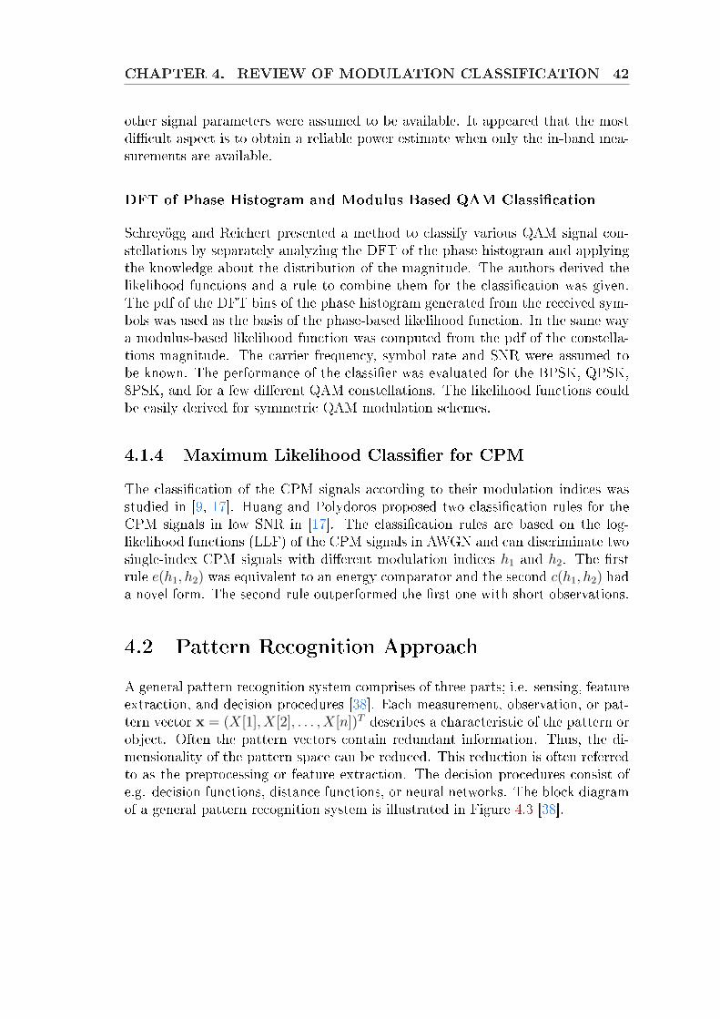
CHAPTER 4. REVIEW OF MODULATION CLASSIFICATION 42
other signal parameters were assumed to be available. It appeared that the mostdicult aspect is to obtain a reliable power estimate when only the in-band mea-surements are available.
DFT of Phase Histogram and Modulus Based QAM Classication
Schreyögg and Reichert presented a method to classify various QAM signal con-stellations by separately analyzing the DFT of the phase histogram and applyingthe knowledge about the distribution of the magnitude. The authors derived thelikelihood functions and a rule to combine them for the classication was given.The pdf of the DFT bins of the phase histogram generated from the received sym-bols was used as the basis of the phase-based likelihood function. In the same waya modulus-based likelihood function was computed from the pdf of the constella-tions magnitude. The carrier frequency, symbol rate and SNR were assumed tobe known. The performance of the classier was evaluated for the BPSK, QPSK,8PSK, and for a few dierent QAM constellations. The likelihood functions couldbe easily derived for symmetric QAM modulation schemes.
4.1.4 Maximum Likelihood Classier for CPMThe classication of the CPM signals according to their modulation indices wasstudied in [9, 17]. Huang and Polydoros proposed two classication rules for theCPM signals in low SNR in [17]. The classication rules are based on the log-likelihood functions (LLF) of the CPM signals in AWGN and can discriminate twosingle-index CPM signals with dierent modulation indices h1 and h2. The rstrule e(h1, h2) was equivalent to an energy comparator and the second c(h1, h2) hada novel form. The second rule outperformed the rst one with short observations.
4.2 Pattern Recognition ApproachA general pattern recognition system comprises of three parts; i.e. sensing, featureextraction, and decision procedures [38]. Each measurement, observation, or pat-tern vector x = (X[1], X[2], . . . , X[n])T describes a characteristic of the pattern orobject. Often the pattern vectors contain redundant information. Thus, the di-mensionality of the pattern space can be reduced. This reduction is often referredto as the preprocessing or feature extraction. The decision procedures consist ofe.g. decision functions, distance functions, or neural networks. The block diagramof a general pattern recognition system is illustrated in Figure 4.3 [38].
CHAPTER 4. REVIEW OF MODULATION CLASSIFICATION 43
SENSING(measuring)
Signal classesPattern
DECISIONvectorsFeature
FEATUREEXTRACTION(preprocessing)
Measurements
x
Figure 4.3: General pattern recognition system.
4.2.1 Envelope Based MethodsRatio of Dierent Envelope Statistics
In [7], Chan and Gadbois proposed a classier based on the ratio (R) of the varianceof the envelope to the square of the mean of the envelope. The authors derivedthe equations for R for four modulation types as a function of the carrier to noiseratio to set up the classication scheme. The classier determines the modulationtype according to the domain R falls in. The performance of the classier for FM,AM, DSB, and SSB modulated signals was evaluated in a simulation. The authorsconcluded that the scheme is suitable for real time applications since the recordlength required for successful identication and the required computation time areshort.Druckmann, Plotkin and Swamy studied and proposed a number of classicationfeatures in [10]. They presented a dierent method of the envelope extraction,which does not require the computation of the Hilbert transform. In addition toR in [7], the authors introduced four more features based on the analytic envelopeand on the new envelope approximation to classify FM, AM, DSB, and SSB. Thefeatures employ ratios of dierent statistics of these two envelopes. The authorsexamined also the performance of a classication rule which utilizes two featuresand proposed a pair which gained a success rate of 99% in carrier-to-noise ratio(CNR) of 10dB. The proposed method for envelope extraction is neverthelessunsuitable for the complex envelope representation.
Deviations of Instantaneous Properties
Azzouz and Nandi proposed nine features for the recognition of the analog anddigital modulations in [3, 4, 27]. The features were derived from the signal spec-trum and the instantaneous amplitude, frequency and phase. The features wereused to classify analog AM, FM, DSB, USB, LSB, and digital 2ASK, 4ASK, 2PSK,4PSK, 2FSK, 4FSK. Usually the classication of the 2PSK and 2ASK is impossiblebecause the commonly used constellations of the 2PSK and 2ASK are identical.The authors used two dierent approaches in classifying the modulated signals.The rst approach was a decision theoretic tree classier where each feature wastested against a certain threshold value at a time. The success rate of the treeclassier depends on the order of the features tested in these branches. The secondapproach was based on an articial neural network. In this approach, all featuresare considered simultaneously which should imply a better performance.
CHAPTER 4. REVIEW OF MODULATION CLASSIFICATION 44
4.2.2 Higher-Order MethodsEven Moment Based MPSK Classier
Soliman and Hsue developed an automatic classication algorithm for carrier wave(CW) and M-ary PSK signals utilizing the statistical moments of the phase com-ponent of the received signal in [36]. Yang and Soliman also studied the moment-based classiers in [42]. In [36], the authors showed that for MPSK signals, evenmoments of the phase component are monotonic increasing functions of M. Basedon this property, the authors formulated a general hypothesis test, developed adecision rule, and derived an analytic expression for the probability of the mis-classication. At low carrier-to-noise ratio (CNR), the authors established thatthe eighth-moment is adequate for classifying the BPSK signals with a reasonableperformance. Finally, the authors compared the performance of the suggestedalgorithm to the quasi log-likelihood ratio (qLLRC), square-law (SLC), and thephase-based (PBC) classiers [20]. The suggested algorithm was outperformed bythe qLLRC algorithm at low CNR but had a comparable performance to the SLCand was better than the PBC algorithms.
The M th-law Based Classier
Reichert [34] presented a classication method which utilizes dierent nonlineari-ties, i.e. squaring and fourth-power, applied to the pre-envelope of the digital mod-ulated signal. The method exploited the dierences in the higher-order moment-spaces of the discrete-time modulating process. These dierences contributed linesin the spectrum of the transformed signal, associated with the unknown carrier fre-quency fc and symbol rate fs. The spectral lines were detected by a periodogramanalysis. Their existence, position and amplitude served as a robust feature forclassifying the 2ASK, 2PSK, 4PSK, MSK, and 2FSK modulated signals. The au-thor carried out a complete statistical analysis of the classication performancein terms of the probability of the detection and false alarm rate. The analyti-cal performance gures were veried with simulated data. Minor defects of thismethod are the complexity of the periodogram analysis and its unsuitability forthe complex envelope representation.
Cyclic Multi-correlation Based MPSK Classier
In [25, 26], Marchand, Le Martret and Lacoume proposed a multiple hypothesisQAM modulation classier designed in the framework of decision theory. Samefeatures were also introduced by Le Martret and Boiteau [22] in a slightly dierentframework. The proposed feature was composed of a combination between fourth-order and squared second-order cyclic temporal cumulants. The combination be-tween the cumulants of dierent orders was intended to bypass the uncertainty
CHAPTER 4. REVIEW OF MODULATION CLASSIFICATION 45
about the power of the signal of interest. The authors presented performance sim-ulations in the context of 4QAM, 16QAM, and 64QAM classication. Comprehen-sive Monte-Carlo simulations for SNR values 5dB and 10dB were performed andthe probability of the correct classication was examined. The classier exhibitedpoor performance for sample sizes less than 1024 symbols. The authors concludedthat the feature introduced in their paper is the only one that can achieve QAMmodulation classication in a cyclostationary context.
4.2.3 Other MethodsClassication Exploiting Zero-Crossings
Hsue and Soliman developed a classier using zero-crossing techniques in [15] andreported the same results a year later in [16]. The zero-crossing sampler had theadvantage of providing accurate phase transition information over a wide dynamicfrequency range. The authors estimated the zero-crossing variance, carrier-to-noiseratio (CNR), and carrier frequency by using these techniques. The phase dierenceand zero-crossing interval histograms were used as the features for recognition ofthe CW, MPSK, and MFSK modulated signals. The obtained simulation resultsshowed that a reasonable average probability of correct classication was achiev-able for CNR≥ 15dB. However, these techniques are unsuitable for the complexenvelope representation.
Classication Based on Distance Functions
Huo and Donoho developed a classication algorithm which used the counts ofthe signals falling into dierent parts of the signal plane as a feature in [18].The feature was far more easier to compute and much faster than the likelihoodmethods and methods based on higher-order statistics. The optimal partition ofthe signal plane was derived for two candidate modulation types by maximizingthe Hellinger distance in the multinomial distribution situation. The performanceof the algorithm was veried with a classier implemented for the 4QAM versus6PSK case. The proposed algorithm was thus dependent on the orientation of thesymbols in the signal space and could only be used for binary classication.
Classication Based on the Modulation Model
Assaleh, Farrell and Mammone proposed a new method for the modulation clas-sication of the digital modulated signals [2]. The method utilized a signal rep-resentation known as the modulation model which is convenient for subsequentanalysis such as the estimation of modulation parameters. The modulation modelwas formed via autoregressive spectrum modeling. It used the instantaneous fre-quency and band-width parameters as obtained from the roots of the autoregressive
CHAPTER 4. REVIEW OF MODULATION CLASSIFICATION 46
polynomial. In particular, the band-width parameter and the derivative of the in-stantaneous frequency were shown to provide excellent measures for informationtype and rate in addition to being noise robust. The method showed excellentpreliminary results. The applicability of this method for the complex enveloperepresentation was not studied.
Classication of CPM
Chung and Polydoros proposed two envelope-based classiers for 2CPFSK signals[9]. The classier was developed for both the single and multi-index CPM signals.The classiers were based on the sum of the squared envelopes (SOSE). In therst method, an appropriately adjusted threshold was able to classify a varietyof candidate modulation sets. The second method could be used with inniteindex sets and was based on an approximate maximum likelihood estimate of theindex pattern derived from SOSE. The binary SOSE scheme was compared to anLLF based method in [17]. The latter outperformed the SOSE scheme but all themethods worked reliably at very low SNR.
Chapter 5
Implemented Methods
In this chapter, we present the methods implemented in this study and the setupused in the simulations. The implemented methods are described in more detailcompared to the previous chapter. The pros and cons of these methods are dis-cussed. We introduce a new feature derived in Appendix A, and its theoreticaldiscrimination ability is discussed. The test signal generation is described as well.
5.1 Test Signal Generation for the SimulationsDierent modulated signals were generated to study some of the methods presentedin this thesis. The modulation types were restricted to the types commonly used inradio communication. In the case of digital modulation, small constellations wereused. To save the required amount of memory and to lower the sampling rate, thecomplex envelope was chosen as the signal representation. The modulation wascarried out by using Matlab functions in Communications Toolbox.In the analog modulation, the modulating signal was a segment of narrow-bandspeech with sampling rate fs = 8kHz. First the modulating signal was re-sampledto fs = 100kHz and it was modulated with the carrier frequency fc = 25kHz.The speech signal was continuous but it cannot be expected to be stationary fora long period of time. Therefore, the results might be much dierent comparedto those obtained with simulated modulating signals. The frequency deviationused in the frequency modulation was chosen to be f∆ = 20kHz. The modulationdepth used in the amplitude modulation was chosen to be the maximum absolutevalue of the modulating signal to avoid any phase shifts. The analog modulationtypes produced for the simulations were AM, FM, DSB, and LSB.The digital modulated signals were obtained similarly to the analog modulation.Uniformly distributed discrete symbol sequences were modulated by the Matlabfunctions. Due to many source coding techniques, the digital bit sequences areuncorrelated. There is, though, some redundancy added by the channel codingbut uniformly distributed random sequences of symbols were used as a modulating
CHAPTER 5. IMPLEMENTED METHODS 48
signal. The digital modulation types produced for the simulations were 2PSK,4PSK, 8PSK, 2FSK, 4FSK, and 8FSK. A plain carrier wave (CW) was also usedfor the generality since it can be regarded as 1PSK or 1FSK. The symbol rate waschosen to be fd = 2500Hz because it should be an integer factor of the samplingrate. The phase states used in the generation of the 2PSK signals were φ = 0 andφ = π. For the 4PSK signals, the phase states were φ = 0, φ = π/2, φ = π, andφ = −π/2. The frequency deviation for the 2FSK signals was f∆ = 2500Hz, andf∆ = 1250Hz for the 4FSK signals.Additive white Gaussian noise (AWGN) was added to the modulated signals beforeconversion to the complex envelope representation. The signal-to-noise ratio (SNR)is dened as a ratio of the power of the signal to the power of the noise and it isusually expressed in decibels. The power of the signal s[k] can be estimated by itsvariance σ2
s . First a normally distributed random sequence w[k] with zero-meanand unit-variance was generated by using a Matlab function. To obtain certainSNR, the noise sequence must be scaled by a constant,
c =
√σ2
s
σ2w10SNR/10
, (5.1)
where σ2w is the variance of the original noise sequence. The noisy signal is then
r[k] = s[k] + cw[k].The complex envelope was obtained by Hilbert transforming the noisy signal byusing a Matlab function. The transformed signal was then multiplied by an expo-nential factor e−jωck/fs , where the angular frequency of the carrier is ωc = 2πfc.The obtained signal was then re-sampled to fs = 50kHz, which performed theband-limitation simultaneously.
5.2 Implemented Methods
5.2.1 Ratio of Variance to Squared MeanThis method for the analog modulation classication is reviewed in Section 4.2.1.The received signal is modeled in the identication scheme [7] as
r(t) = x(t) + w(t), (5.2)
where the signal x(t) has an unknown modulation type to be determined and w(t)is a stationary, Gaussian white noise sequence with variance σ2
w and uncorrelatedwith x(t). The analytic envelope used in this method is dened as
ξ(t) = r2(t) + r2(t), (5.3)
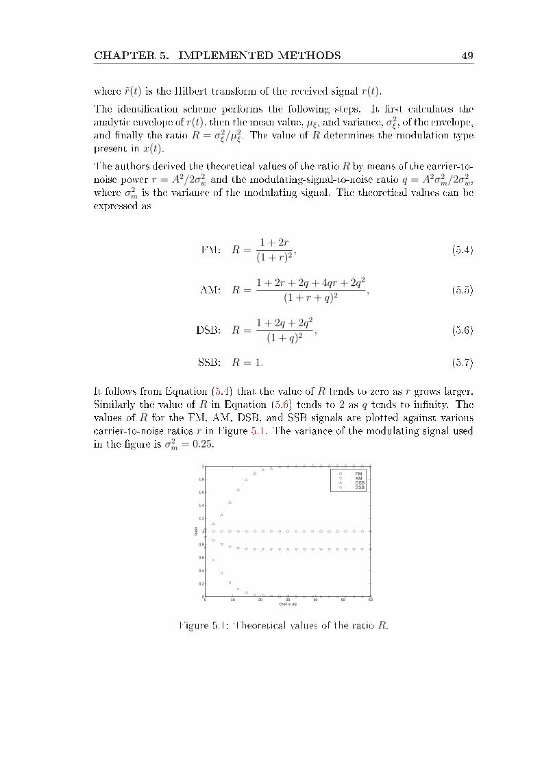
CHAPTER 5. IMPLEMENTED METHODS 49
where r(t) is the Hilbert transform of the received signal r(t).The identication scheme performs the following steps. It rst calculates theanalytic envelope of r(t), then the mean value, µξ, and variance, σ2
ξ , of the envelope,and nally the ratio R = σ2
ξ/µ2ξ . The value of R determines the modulation type
present in x(t).The authors derived the theoretical values of the ratio R by means of the carrier-to-noise power r = A2/2σ2
w and the modulating-signal-to-noise ratio q = A2σ2m/2σ2
w,where σ2
m is the variance of the modulating signal. The theoretical values can beexpressed as
FM: R =1 + 2r
(1 + r)2, (5.4)
AM: R =1 + 2r + 2q + 4qr + 2q2
(1 + r + q)2, (5.5)
DSB: R =1 + 2q + 2q2
(1 + q)2, (5.6)
SSB: R = 1. (5.7)
It follows from Equation (5.4) that the value of R tends to zero as r grows larger.Similarly the value of R in Equation (5.6) tends to 2 as q tends to innity. Thevalues of R for the FM, AM, DSB, and SSB signals are plotted against variouscarrier-to-noise ratios r in Figure 5.1. The variance of the modulating signal usedin the gure is σ2
m = 0.25.
0 10 20 30 40 50 600
0.2
0.4
0.6
0.8
1
1.2
1.4
1.6
1.8
2
CNR in dB
Rat
io
FMAMDSBSSB
Figure 5.1: Theoretical values of the ratio R.
CHAPTER 5. IMPLEMENTED METHODS 50
5.2.2 Deviations in Instantaneous PropertiesAnother approach for the analog modulation classication is introduced in Section4.2.1. Key features γmax, σap, σdp, and P are used to classify analog modulatedsignals. The key feature γmax represents the maximum value of the spectral powerdensity of the normalized centered instantaneous amplitude acn[k] of the receivedsignal. The value of γmax can be obtained by the maximum value of the DFTsequence of acn[k] as follows
γmax = max∣∣DFT [acn[k]]
∣∣2/Ns = maxn
∣∣∣Ns−1∑
k=0
acn[k]e−jkn2π/Ns
∣∣∣2
/Ns, (5.8)
where Ns is the number of the samples in a segment. By the Parseval's theoremthe power spectral density is equivalent to the square of the absolute values of theDFT sequence.Another key feature σap is the standard deviation of the absolute value of thecentered nonlinear component of the instantaneous phase evaluated over the non-weak intervals of a signal segment. The non-weak intervals are dened as theindices for which the normalized amplitude exceeds a certain threshold an[k] > at.The estimation of the instantaneous phase is very sensitive to noise below thatthreshold. The value of σap can be obtained as follows
σap =
√1
C
( ∑
an[k]>at
φ2NL[k]
)−
( 1
C
∑
an[k]>at
|φNL[k]|)2
, (5.9)
where C is the number of the samples φNL[k] for which an[k] > at.The key feature σdp is the standard deviation of the centered nonlinear componentof the direct instantaneous phase, evaluated over the non-weak intervals of a signalsegment. Similarly, σdp is dened by
σdp =
√1
C
( ∑
an[k]>at
φ2NL[k]
)−
( 1
C
∑
an[k]>at
φNL[k])2
. (5.10)
The key feature P measures the spectrum symmetry about the carrier frequencyand is calculated by the dierence of the power in the upper and lower-sidebandsnormalized by the total power. In the case of the complex envelope signal, thecarrier frequency fc = 0. The key feature P can be expressed as
P =PL − PU
PL + PU
, (5.11)
CHAPTER 5. IMPLEMENTED METHODS 51
where
PL =
fcn∑n=1
|X[n]|2, and PU =
2fcn+1∑
n=fcn+2
|X[n]|2. (5.12)
In Equation (5.11), X[n] is the DFT sequence of the signal x[k] and fcn + 1 is thesample number corresponding to the carrier frequency as follows
X(n) =Ns−1∑
k=0
x[k]e−jkn2π/Ns , and fcn =fcNs
fs
− 1. (5.13)
Key features γmax, σap, σdp, σaa, and σaf are used in classication of the digitalmodulated signals. Key feature σaa is the standard deviation of the absolute valueof the normalized centered instantaneous amplitude of a signal segment. Similarly,σaa is dened by
σaa =
√√√√ 1
Ns
( Ns∑
k=1
a2cn[k]
)−
( 1
Ns
Ns∑
k=1
|acn[k]|)2
. (5.14)
The key feature σaf is the standard deviation of the absolute value of the normal-ized centered instantaneous frequency, evaluated over the non-weak intervals of asignal segment. Similarly, σaf is dened by
σaf =
√1
C
( ∑
an[k]>at
f 2N [k]
)−
( 1
C
∑
an[k]>at
|fN [k]|)2
. (5.15)
All the previous features and three new features are used to classify both theanalog and digital modulated signals. The key feature σa is the standard deviationof the normalized centered instantaneous amplitude, evaluated over the non-weakintervals of a signal segment. It is dened by
σa =
√1
C
( ∑
an[k]>at
a2cn[k]
)−
( 1
C
∑
an[k]>at
acn[k])2
. (5.16)
The key feature µa42 is the kurtosis of the normalized centered instantaneous am-
plitude and is dened by
µa42 =
E[a4cn(t)](
E[a2cn(t)]
)2 , (5.17)
which is another denition of the kurtosis than the one given in Section 3.2.2. Thisfeature was used to discriminate the analog and digital amplitude modulations AM,
CHAPTER 5. IMPLEMENTED METHODS 52
2ASK, and 4ASK. In the simulation part, we have not used any ASK modulatedsignals. Therefore this feature is not used in the implementation.The key feature µf
42 is the kurtosis of the normalized centered instantaneous fre-quency and is dened by
µf42 =
E[f 4N(t)](
E[f 2N(t)]
)2 . (5.18)
This feature was used to discriminate FM, 2FSK, and 4FSK.
5.2.3 Even Moments of MPSK SignalsThis method is presented in Section 4.2.2. In [36], the phase of the received signalis extracted by the methods given in Section 2.1. For a signal contaminated byAWGN, the extracted phase can be represented as
φα[k] = θα[k] + v[k], −π < φα[k] ≤ π, (5.19)
where θα[k] is the sampled phase component of the transmitted MPSK signal, andv[k] is the contribution of the noise and any other measurement error. Without lossof generality, φα[k] and θα[k] are assumed independent and identically distributed(i.i.d.) with zero-means. The number of the symbols is given by M = 2α, α =0, 1, 2, . . . , where α = 0 corresponds to a CW signal. For the CW signal (α = 0),the pdf of the phase is given as
fφ(φ0) =e−γ
2π+
√γ
πcos(φ0)e
−γ sin2(φ0)Q[−
√2γ cos(φ0)
], −π < φ0 ≤ π,
where
Q[x] =1√2π
∫ ∞
x
e−y2/2dy and γ =A2
2σ2w
, (5.20)
and A is the amplitude of the transmitted CW signal, and σ2w is the noise variance.
Due to the complicated nature of Equation (5.20), it can be approximated by theTikhonov pdf given as
fφ(φ0) ' exp[2γ cos(φ0)]
2πI0[2γ], −π < φ0 ≤ π, (5.21)
CHAPTER 5. IMPLEMENTED METHODS 53
where I0[·] is the zero-order modied Bessel function of the rst kind. The pdf ofθα can be written as
fθ(y; α) =1
2α
2α∑
k=1
δ[y − ηk(α)], (5.22)
where ηk(α) is given as
ηk(α) =2k − 2α − 1
2α, k = 1, 2, . . . , 2α, α = 0, . . . , log2 M. (5.23)
By combining Equations (5.19), (5.21), and (5.22) we obtain the pdf fφ(y; α) as asum of non-central Tikhonov functions, which can be expressed as
fφ(y; α) =1
2α
2α∑
k=1
exp[2γ cos(y − ηk(α))]
2πI0[2γ]. (5.24)
The approximations of fφ(y; α) for α = 0, 1, 2, 3 obtained from the histograms ofthe simulated signals are given in Figure 5.2. The number of the peaks in thegures indicate the number of the signal phase states. As SNR decreases, thepeaks smear o and nally the pdf approaches that of a uniformly distributedrandom variable. As shown in Figure 5.2, for large α, fφ(y; α) is atter than thosewith small α and fφ(y; α) will approach 1/2π as SNR → −∞ dB or α →∞.In the presence of noise, the nth-order moment of φα is given in Equation (5.25).The authors proved a theorem which states that the even moments mn(α) ofthe phase of the MPSK signals are monotonic increasing functions of α whereα = 0, 1, . . . , log2 M .
mn(α) =
∫ π
−pi
ynfφ(y; α)dy (5.25)
=
12α+1πI0[2γ]
∑2α
i=1−π
∫ π
−πyn exp[2γ cos(y − ηi(α))]dy, n even
0, n odd
Figure 5.3 shows the moments of MPSK signals at SNR = 8 dB. The values aregiven in a logarithmic scale. The gure shows also that as α grows the dierencemn(α + 1) − mn(α) gets smaller and higher-order moments may be needed todiscriminate between the signals with large M.
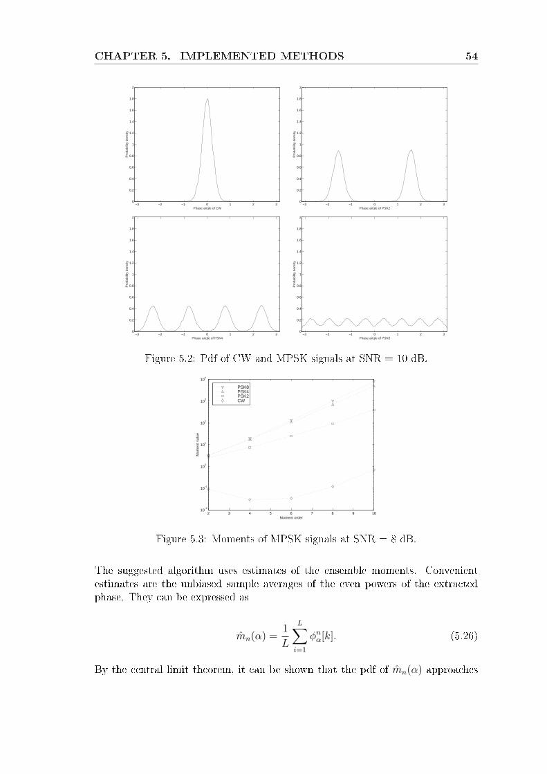
CHAPTER 5. IMPLEMENTED METHODS 54
−3 −2 −1 0 1 2 30
0.2
0.4
0.6
0.8
1
1.2
1.4
1.6
1.8
2
Phase angle of CW
Pro
babi
lity
dens
ity
−3 −2 −1 0 1 2 30
0.2
0.4
0.6
0.8
1
1.2
1.4
1.6
1.8
2
Phase angle of PSK2
Pro
babi
lity
dens
ity
−3 −2 −1 0 1 2 30
0.2
0.4
0.6
0.8
1
1.2
1.4
1.6
1.8
2
Phase angle of PSK4
Pro
babi
lity
dens
ity
−3 −2 −1 0 1 2 30
0.2
0.4
0.6
0.8
1
1.2
1.4
1.6
1.8
2
Phase angle of PSK8
Pro
babi
lity
dens
ity
Figure 5.2: Pdf of CW and MPSK signals at SNR = 10 dB.
2 3 4 5 6 7 8 9 1010
−2
10−1
100
101
102
103
104
Moment order
Mom
ent v
alue
PSK8PSK4PSK2CW
Figure 5.3: Moments of MPSK signals at SNR = 8 dB.
The suggested algorithm uses estimates of the ensemble moments. Convenientestimates are the unbiased sample averages of the even powers of the extractedphase. They can be expressed as
mn(α) =1
L
L∑i=1
φnα[k]. (5.26)
By the central limit theorem, it can be shown that the pdf of mn(α) approaches
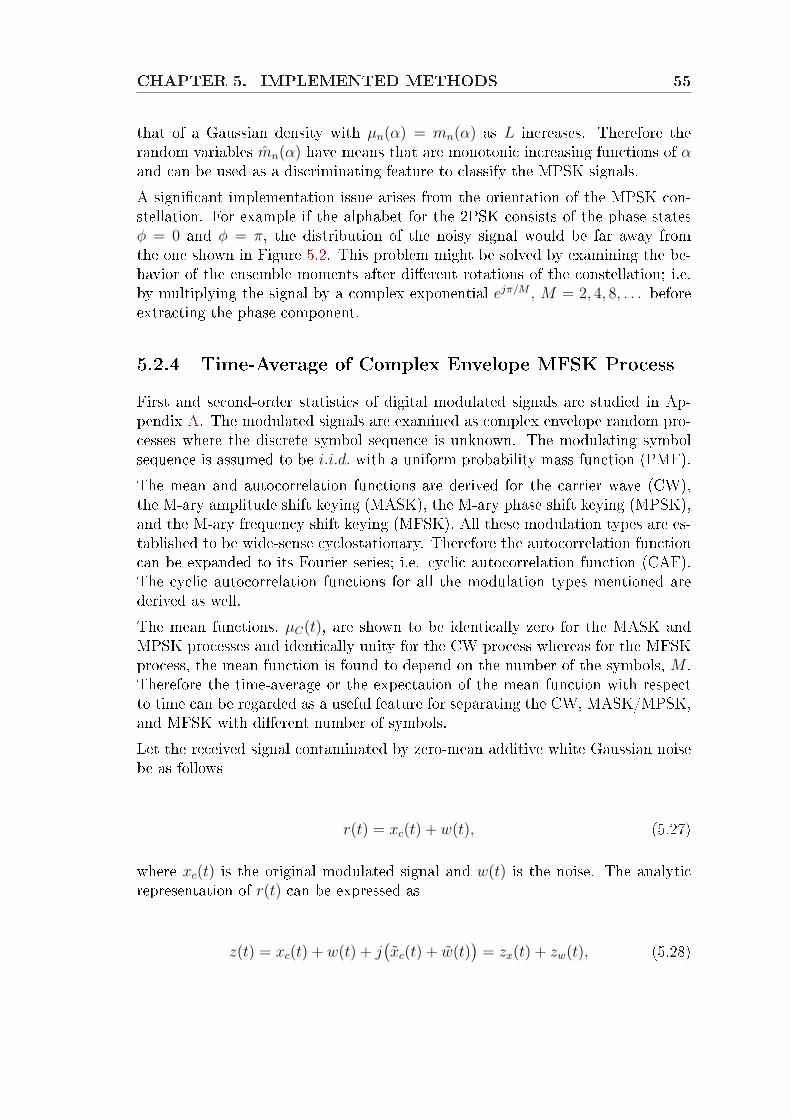
CHAPTER 5. IMPLEMENTED METHODS 55
that of a Gaussian density with µn(α) = mn(α) as L increases. Therefore therandom variables mn(α) have means that are monotonic increasing functions of αand can be used as a discriminating feature to classify the MPSK signals.A signicant implementation issue arises from the orientation of the MPSK con-stellation. For example if the alphabet for the 2PSK consists of the phase statesφ = 0 and φ = π, the distribution of the noisy signal would be far away fromthe one shown in Figure 5.2. This problem might be solved by examining the be-havior of the ensemble moments after dierent rotations of the constellation; i.e.by multiplying the signal by a complex exponential ejπ/M , M = 2, 4, 8, . . . beforeextracting the phase component.
5.2.4 Time-Average of Complex Envelope MFSK ProcessFirst and second-order statistics of digital modulated signals are studied in Ap-pendix A. The modulated signals are examined as complex envelope random pro-cesses where the discrete symbol sequence is unknown. The modulating symbolsequence is assumed to be i.i.d. with a uniform probability mass function (PMF).The mean and autocorrelation functions are derived for the carrier wave (CW),the M-ary amplitude shift keying (MASK), the M-ary phase shift keying (MPSK),and the M-ary frequency shift keying (MFSK). All these modulation types are es-tablished to be wide-sense cyclostationary. Therefore the autocorrelation functioncan be expanded to its Fourier series; i.e. cyclic autocorrelation function (CAF).The cyclic autocorrelation functions for all the modulation types mentioned arederived as well.The mean functions, µC(t), are shown to be identically zero for the MASK andMPSK processes and identically unity for the CW process whereas for the MFSKprocess, the mean function is found to depend on the number of the symbols, M .Therefore the time-average or the expectation of the mean function with respectto time can be regarded as a useful feature for separating the CW, MASK/MPSK,and MFSK with dierent number of symbols.Let the received signal contaminated by zero-mean additive white Gaussian noisebe as follows
r(t) = xc(t) + w(t), (5.27)
where xc(t) is the original modulated signal and w(t) is the noise. The analyticrepresentation of r(t) can be expressed as
z(t) = xc(t) + w(t) + j(xc(t) + w(t)
)= zx(t) + zw(t), (5.28)
CHAPTER 5. IMPLEMENTED METHODS 56
where zx(t) is the analytic representation of the original modulated signal xc(t)and zw(t) is the analytic representation of the noise w(t). In Equation (5.28), wehave used the linearity property of the Hilbert transform. The complex enveloperepresentation of r(t) can be expressed as
c(t) = z(t)e−jωct =[zx(t) + zw(t)
]e−jωct. (5.29)
The time-average of the complex envelope representation of the received signal c(t)can be divided into the time-average of the modulated signal component and thetime-average of the noise component. The time-average of the noise component willbe zero due to the properties of the AWGN, Hilbert transform, and multiplicationby a complex exponential [31, 30]. The time-average of the complex envelope ofr(t) depends only on the time-average of the original modulated signal. Thereforethe time-averages derived for the digital modulated signals in Appendix A can beused as a distinctive feature. These features are summarized in Table 5.1.The ensemble estimate of the time-average is an attractive feature due to its ro-bustness against the zero-mean noise and fast calculation. The number of symbolsrequired for consistent recognition is studied by simulations in the next chapter.The autocorrelation function, RC(t1, t2), is also identically zero for the MPSKprocess when M = 4, 8, 16, . . . and unity for the CW process whereas for theother modulation types mentioned, the autocorrelation function depends on M .The cyclic autocorrelations are found to exhibit similar characteristics. Furtheranalysis is needed to exploit the CAF in the modulation recognition. The featuresof the autocorrelation functions are summarized in Table 5.1, as well.
Table 5.1: Summary of rst and second-order statistics.CW MASK MPSK MFSK
µC 1 0 0 1/MRC(t1, t2) 1 depends on M 0 for M = 4, 8, 16, . . . depends on M
Chapter 6
Simulation Results
In this chapter, the methods reviewed in the previous chapter are simulated. Theresults are given as gures where their discrimination eciency can be seen. Alsothe number of the symbols needed for the discrimination is studied in the case ofthe features used with digital modulation types. In the last section, we discussabout the proper features for our objectives.
6.1 Results
6.1.1 Ratio of Variance to Squared MeanThe R values of the analog modulated signals against the signal-to-noise ratio(SNR) calculated over a segment of 51200 samples are depicted on the left handside of Figure 6.1. The order of dierent modulation types meets the theoreticalvalues reviewed in Section 5.2.1. The actual values are though quite dierent fromthose illustrated in Figure 5.1. This is a consequence of the assumptions madein the derivation of the theoretical values. E.g. it is clear that the variance ofthe modulating signal is not a constant. The modulation types can be separatedpairwise by a single straight line down to about 15dB.The behavior of the feature against the number of the samples at SNR 15dB can beseen on the right hand side of Figure 6.1. Again the order of the modulation typesseems to be correct with a small number of samples but the variance is large. Thevalues converge after 1000 samples and 2048 samples used in the original paper [7]is adequate.
6.1.2 Deviations in Instantaneous PropertiesThe features in [3] are simulated for the analog and digital modulation types.The segment size used was chosen to be 2048; same as in [4, 3]. The key feature
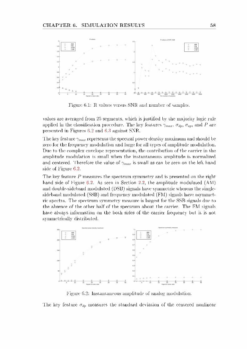
CHAPTER 6. SIMULATION RESULTS 58
0 5 10 15 20 25 30 35 400
0.2
0.4
0.6
0.8
1
1.2
1.4
1.6
1.8
2R values
Signal to noise ratio
AMFMDSBLSB
200 400 600 800 1000 1200 1400 1600 1800 20000
0.5
1
1.5
2
2.5R values at SNR 15dB
The number of samples
AMFMDSBLSB
Figure 6.1: R values versus SNR and number of samples.
values are averaged from 25 segments, which is justied by the majority logic ruleapplied in the classication procedure. The key features γmax, σdp, σap, and P arepresented in Figures 6.2 and 6.3 against SNR.The key feature γmax represents the spectral power density maximum and should bezero for the frequency modulation and large for all types of amplitude modulation.Due to the complex envelope representation, the contribution of the carrier in theamplitude modulation is small when the instantaneous amplitude is normalizedand centered. Therefore the value of γmax is small as can be seen on the left handside of Figure 6.2.The key feature P measures the spectrum symmetry and is presented on the righthand side of Figure 6.2. As seen in Section 2.2, the amplitude modulated (AM)and double-sideband modulated (DSB) signals have symmetric whereas the single-sideband modulated (SSB) and frequency modulated (FM) signals have asymmet-ric spectra. The spectrum symmetry measure is largest for the SSB signals due tothe absence of the other half of the spectrum about the carrier. The FM signalshave always information on the both sides of the carrier frequency but it is notsymmetrically distributed.
5 10 15 20 25 30 35 400
50
100
150
200
250Spectral power density maximum
Signal to noise ratio
AMFMDSBLSB
5 10 15 20 25 30 35 400
0.1
0.2
0.3
0.4
0.5
0.6
0.7
0.8
0.9
1Spectrum symmetry measure
Signal to noise ratio
AMFMDSBLSB
Figure 6.2: Instantaneous amplitude of analog modulation.
The key feature σdp measures the standard deviation of the centered nonlinear
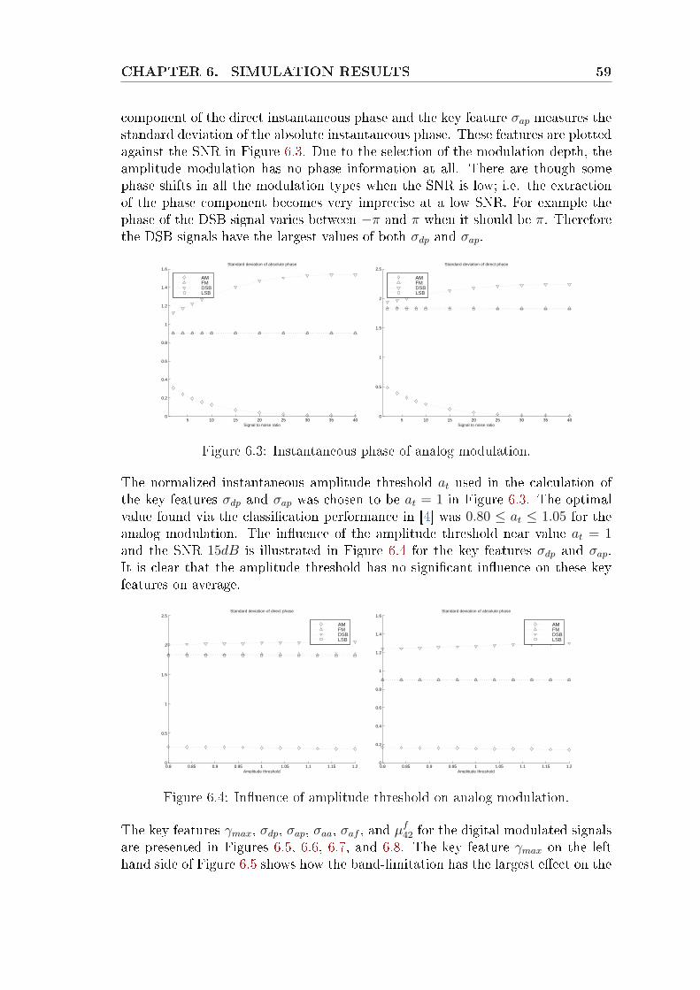
CHAPTER 6. SIMULATION RESULTS 59
component of the direct instantaneous phase and the key feature σap measures thestandard deviation of the absolute instantaneous phase. These features are plottedagainst the SNR in Figure 6.3. Due to the selection of the modulation depth, theamplitude modulation has no phase information at all. There are though somephase shifts in all the modulation types when the SNR is low; i.e. the extractionof the phase component becomes very imprecise at a low SNR. For example thephase of the DSB signal varies between −π and π when it should be π. Thereforethe DSB signals have the largest values of both σdp and σap.
5 10 15 20 25 30 35 400
0.2
0.4
0.6
0.8
1
1.2
1.4
1.6Standard deviation of absolute phase
Signal to noise ratio
AMFMDSBLSB
5 10 15 20 25 30 35 400
0.5
1
1.5
2
2.5Standard deviation of direct phase
Signal to noise ratio
AMFMDSBLSB
Figure 6.3: Instantaneous phase of analog modulation.
The normalized instantaneous amplitude threshold at used in the calculation ofthe key features σdp and σap was chosen to be at = 1 in Figure 6.3. The optimalvalue found via the classication performance in [4] was 0.80 ≤ at ≤ 1.05 for theanalog modulation. The inuence of the amplitude threshold near value at = 1and the SNR 15dB is illustrated in Figure 6.4 for the key features σdp and σap.It is clear that the amplitude threshold has no signicant inuence on these keyfeatures on average.
0.8 0.85 0.9 0.95 1 1.05 1.1 1.15 1.20
0.5
1
1.5
2
2.5Standard deviation of direct phase
Amplitude threshold
AMFMDSBLSB
0.8 0.85 0.9 0.95 1 1.05 1.1 1.15 1.20
0.2
0.4
0.6
0.8
1
1.2
1.4
1.6Standard deviation of absolute phase
Amplitude threshold
AMFMDSBLSB
Figure 6.4: Inuence of amplitude threshold on analog modulation.
The key features γmax, σdp, σap, σaa, σaf , and µf42 for the digital modulated signals
are presented in Figures 6.5, 6.6, 6.7, and 6.8. The key feature γmax on the lefthand side of Figure 6.5 shows how the band-limitation has the largest eect on the
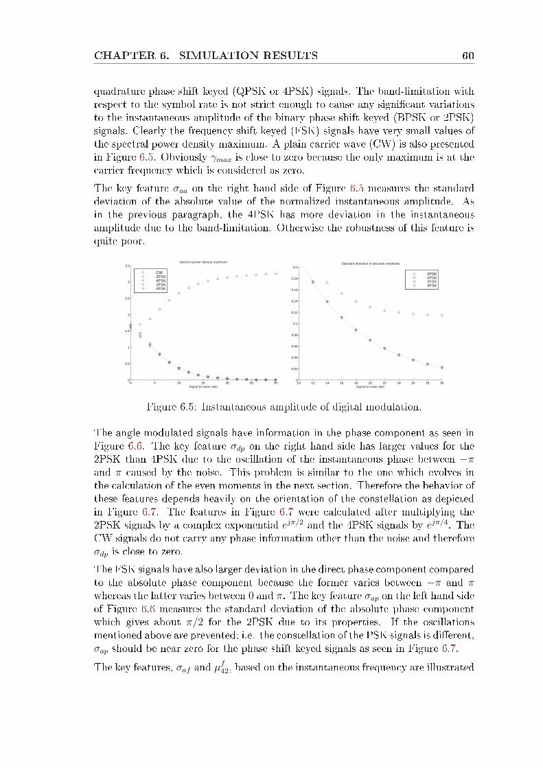
CHAPTER 6. SIMULATION RESULTS 60
quadrature phase shift keyed (QPSK or 4PSK) signals. The band-limitation withrespect to the symbol rate is not strict enough to cause any signicant variationsto the instantaneous amplitude of the binary phase shift keyed (BPSK or 2PSK)signals. Clearly the frequency shift keyed (FSK) signals have very small values ofthe spectral power density maximum. A plain carrier wave (CW) is also presentedin Figure 6.5. Obviously γmax is close to zero because the only maximum is at thecarrier frequency which is considered as zero.The key feature σaa on the right hand side of Figure 6.5 measures the standarddeviation of the absolute value of the normalized instantaneous amplitude. Asin the previous paragraph, the 4PSK has more deviation in the instantaneousamplitude due to the band-limitation. Otherwise the robustness of this feature isquite poor.
0 5 10 15 20 25 300
0.5
1
1.5
2
2.5
3
3.5Spectral power density maximum
Signal to noise ratio
CW2PSK4PSK2FSK4FSK
10 12 14 16 18 20 22 24 26 28 300
0.02
0.04
0.06
0.08
0.1
0.12
0.14
0.16
0.18
0.2Standard deviation of absolute amplitude
Signal to noise ratio
2PSK4PSK2FSK4FSK
Figure 6.5: Instantaneous amplitude of digital modulation.
The angle modulated signals have information in the phase component as seen inFigure 6.6. The key feature σdp on the right hand side has larger values for the2PSK than 4PSK due to the oscillation of the instantaneous phase between −πand π caused by the noise. This problem is similar to the one which evolves inthe calculation of the even moments in the next section. Therefore the behavior ofthese features depends heavily on the orientation of the constellation as depictedin Figure 6.7. The features in Figure 6.7 were calculated after multiplying the2PSK signals by a complex exponential ejπ/2 and the 4PSK signals by ejπ/4. TheCW signals do not carry any phase information other than the noise and thereforeσdp is close to zero.The FSK signals have also larger deviation in the direct phase component comparedto the absolute phase component because the former varies between −π and πwhereas the latter varies between 0 and π. The key feature σap on the left hand sideof Figure 6.6 measures the standard deviation of the absolute phase componentwhich gives about π/2 for the 2PSK due to its properties. If the oscillationsmentioned above are prevented; i.e. the constellation of the PSK signals is dierent,σap should be near zero for the phase shift keyed signals as seen in Figure 6.7.The key features, σaf and µf
42, based on the instantaneous frequency are illustrated
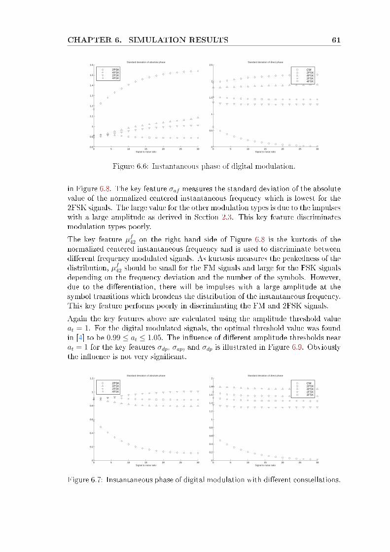
CHAPTER 6. SIMULATION RESULTS 61
0 5 10 15 20 25 300.8
0.9
1
1.1
1.2
1.3
1.4
1.5
1.6Standard deviation of absolute phase
Signal to noise ratio
2PSK4PSK2FSK4FSK
0 5 10 15 20 25 300
0.5
1
1.5
2
2.5Standard deviation of direct phase
Signal to noise ratio
CW2PSK4PSK2FSK4FSK
Figure 6.6: Instantaneous phase of digital modulation.
in Figure 6.8. The key feature σaf measures the standard deviation of the absolutevalue of the normalized centered instantaneous frequency which is lowest for the2FSK signals. The large value for the other modulation types is due to the impulseswith a large amplitude as derived in Section 2.3. This key feature discriminatesmodulation types poorly.The key feature µf
42 on the right hand side of Figure 6.8 is the kurtosis of thenormalized centered instantaneous frequency and is used to discriminate betweendierent frequency modulated signals. As kurtosis measures the peakedness of thedistribution, µf
42 should be small for the FM signals and large for the FSK signalsdepending on the frequency deviation and the number of the symbols. However,due to the dierentiation, there will be impulses with a large amplitude at thesymbol transitions which broadens the distribution of the instantaneous frequency.This key feature performs poorly in discriminating the FM and 2FSK signals.Again the key features above are calculated using the amplitude threshold valueat = 1. For the digital modulated signals, the optimal threshold value was foundin [4] to be 0.99 ≤ at ≤ 1.05. The inuence of dierent amplitude thresholds nearat = 1 for the key features σdp, σap, and σdp is illustrated in Figure 6.9. Obviouslythe inuence is not very signicant.
0 5 10 15 20 25 300
0.2
0.4
0.6
0.8
1
1.2Standard deviation of absolute phase
Signal to noise ratio
2PSK4PSK2FSK4FSK
0 5 10 15 20 25 300
0.2
0.4
0.6
0.8
1
1.2
1.4
1.6
1.8
2Standard deviation of direct phase
Signal to noise ratio
CW2PSK4PSK2FSK4FSK
Figure 6.7: Instantaneous phase of digital modulation with dierent constellations.
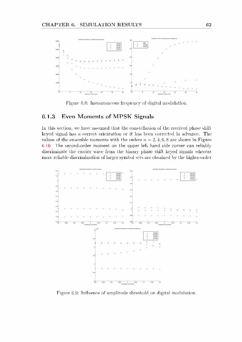
CHAPTER 6. SIMULATION RESULTS 62
0 5 10 15 20 25 300
1000
2000
3000
4000
5000
6000Standard deviation of absolute frequency
Signal to noise ratio
2PSK4PSK2FSK4FSK
0 5 10 15 20 25 300
5
10
15
20
25
30Kurtosis of the instantaneous frequency
Signal to noise ratio
FM2FSK4FSK
Figure 6.8: Instantaneous frequency of digital modulation.
6.1.3 Even Moments of MPSK SignalsIn this section, we have assumed that the constellation of the received phase shiftkeyed signal has a correct orientation or it has been corrected in advance. Thevalues of the ensemble moments with the orders n = 2, 4, 6, 8 are shown in Figure6.10. The second-order moment on the upper left hand side corner can reliablydiscriminate the carrier wave from the binary phase shift keyed signals whereasmore reliable discrimination of larger symbol sets are obtained by the higher-order
0.8 0.85 0.9 0.95 1 1.05 1.1 1.15 1.21.2
1.3
1.4
1.5
1.6
1.7
1.8
1.9
2
2.1
2.2Standard deviation of direct phase
Amplitude threshold
2PSK4PSK2FSK4FSK
0.8 0.85 0.9 0.95 1 1.05 1.1 1.15 1.20.8
0.9
1
1.1
1.2
1.3
1.4
1.5
1.6Standard deviation of absolute phase
Amplitude threshold
2PSK4PSK2FSK4FSK
0.8 0.85 0.9 0.95 1 1.05 1.1 1.15 1.20
0.5
1
1.5
2
2.5
3x 10
4 Standard deviation of absolute frequency
Amplitude threshold
2PSK4PSK2FSK4FSK
Figure 6.9: Inuence of amplitude threshold on digital modulation.
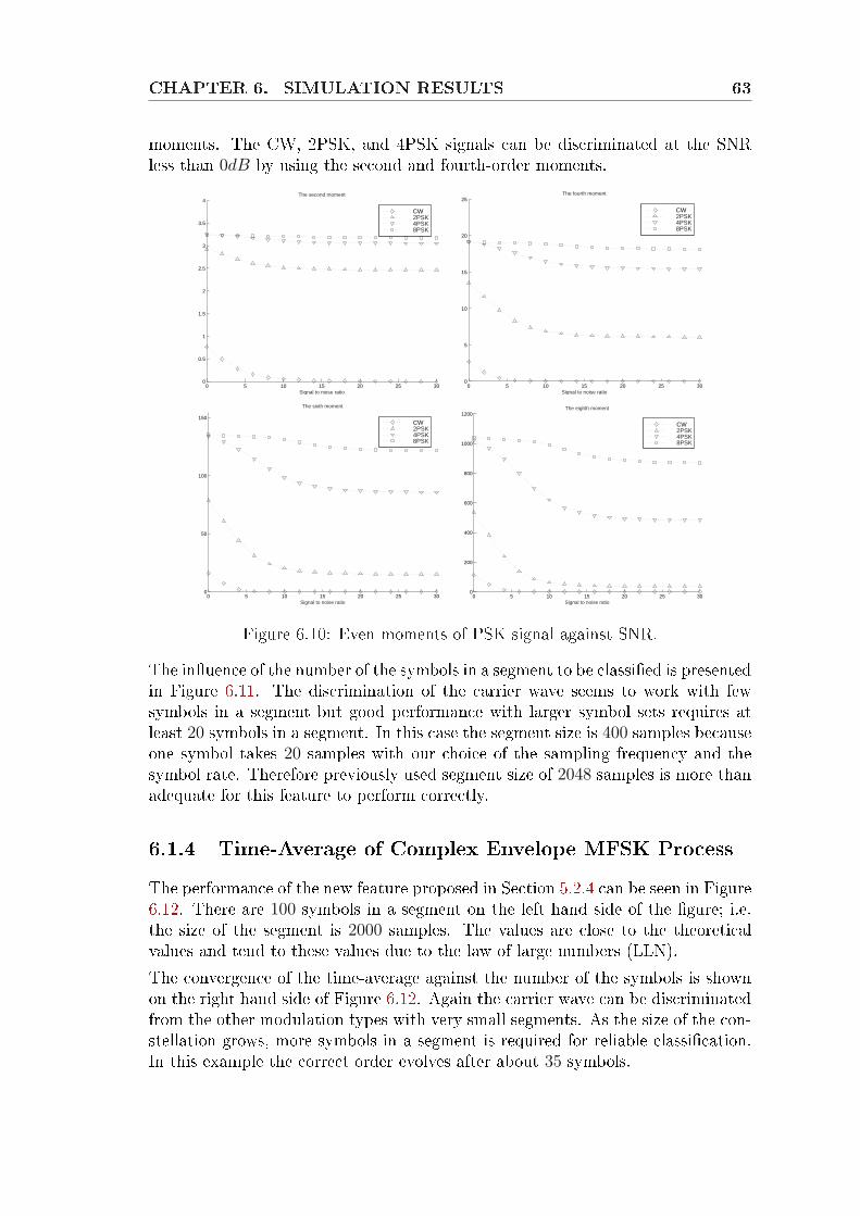
CHAPTER 6. SIMULATION RESULTS 63
moments. The CW, 2PSK, and 4PSK signals can be discriminated at the SNRless than 0dB by using the second and fourth-order moments.
0 5 10 15 20 25 300
0.5
1
1.5
2
2.5
3
3.5
4The second moment
Signal to noise ratio
CW2PSK4PSK8PSK
0 5 10 15 20 25 300
5
10
15
20
25The fourth moment
Signal to noise ratio
CW2PSK4PSK8PSK
0 5 10 15 20 25 300
50
100
150
The sixth moment
Signal to noise ratio
CW2PSK4PSK8PSK
0 5 10 15 20 25 300
200
400
600
800
1000
1200The eighth moment
Signal to noise ratio
CW2PSK4PSK8PSK
Figure 6.10: Even moments of PSK signal against SNR.
The inuence of the number of the symbols in a segment to be classied is presentedin Figure 6.11. The discrimination of the carrier wave seems to work with fewsymbols in a segment but good performance with larger symbol sets requires atleast 20 symbols in a segment. In this case the segment size is 400 samples becauseone symbol takes 20 samples with our choice of the sampling frequency and thesymbol rate. Therefore previously used segment size of 2048 samples is more thanadequate for this feature to perform correctly.
6.1.4 Time-Average of Complex Envelope MFSK ProcessThe performance of the new feature proposed in Section 5.2.4 can be seen in Figure6.12. There are 100 symbols in a segment on the left hand side of the gure; i.e.the size of the segment is 2000 samples. The values are close to the theoreticalvalues and tend to these values due to the law of large numbers (LLN).The convergence of the time-average against the number of the symbols is shownon the right hand side of Figure 6.12. Again the carrier wave can be discriminatedfrom the other modulation types with very small segments. As the size of the con-stellation grows, more symbols in a segment is required for reliable classication.In this example the correct order evolves after about 35 symbols.
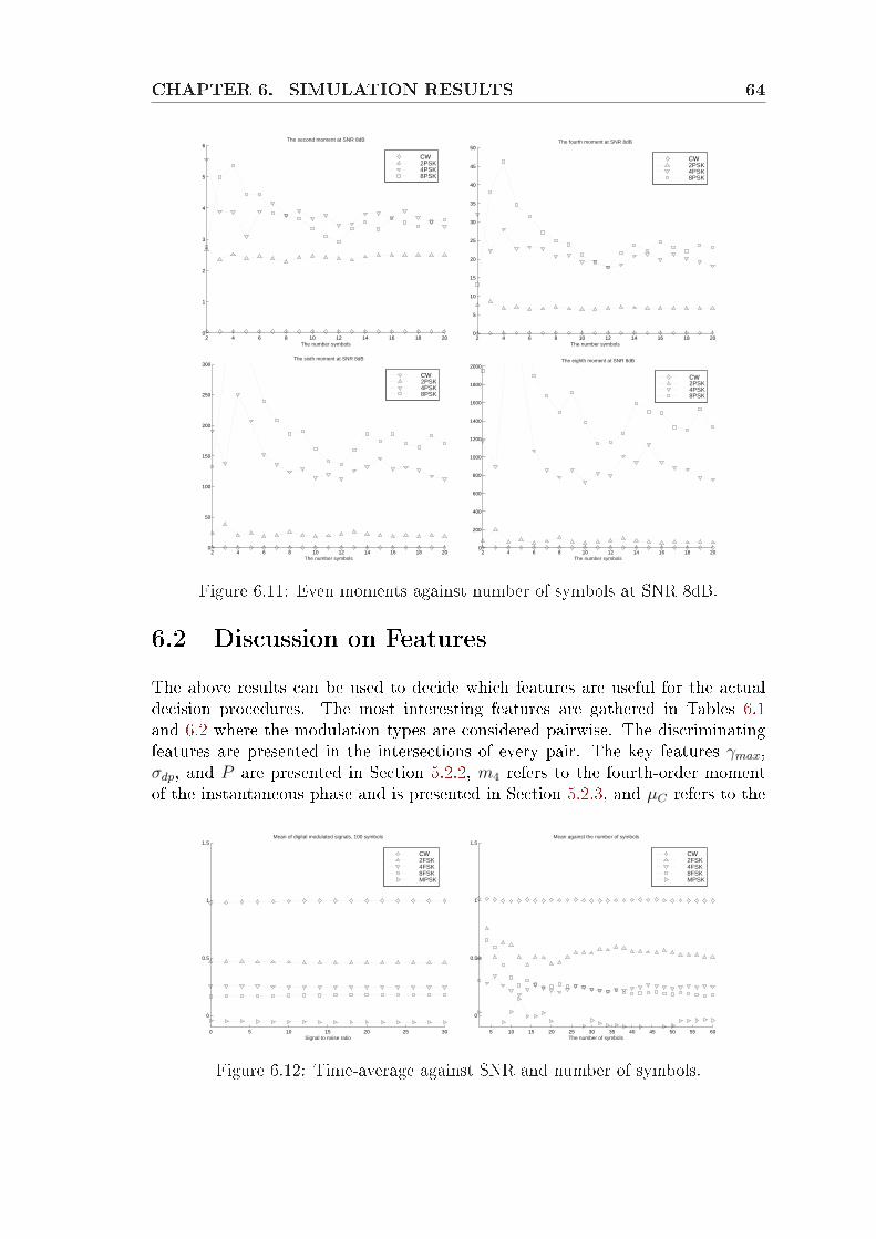
CHAPTER 6. SIMULATION RESULTS 64
2 4 6 8 10 12 14 16 18 200
1
2
3
4
5
6The second moment at SNR 8dB
The number symbols
CW2PSK4PSK8PSK
2 4 6 8 10 12 14 16 18 200
5
10
15
20
25
30
35
40
45
50The fourth moment at SNR 8dB
The number symbols
CW2PSK4PSK8PSK
2 4 6 8 10 12 14 16 18 200
50
100
150
200
250
300The sixth moment at SNR 8dB
The number symbols
CW2PSK4PSK8PSK
2 4 6 8 10 12 14 16 18 200
200
400
600
800
1000
1200
1400
1600
1800
2000The eighth moment at SNR 8dB
The number symbols
CW2PSK4PSK8PSK
Figure 6.11: Even moments against number of symbols at SNR 8dB.
6.2 Discussion on FeaturesThe above results can be used to decide which features are useful for the actualdecision procedures. The most interesting features are gathered in Tables 6.1and 6.2 where the modulation types are considered pairwise. The discriminatingfeatures are presented in the intersections of every pair. The key features γmax,σdp, and P are presented in Section 5.2.2, m4 refers to the fourth-order momentof the instantaneous phase and is presented in Section 5.2.3, and µC refers to the
0 5 10 15 20 25 30
0
0.5
1
1.5Mean of digital modulated signals, 100 symbols
Signal to noise ratio
CW2FSK4FSK8FSKMPSK
5 10 15 20 25 30 35 40 45 50 55 60
0
0.5
1
1.5Mean against the number of symbols
The number of symbols
CW2FSK4FSK8FSKMPSK
Figure 6.12: Time-average against SNR and number of symbols.
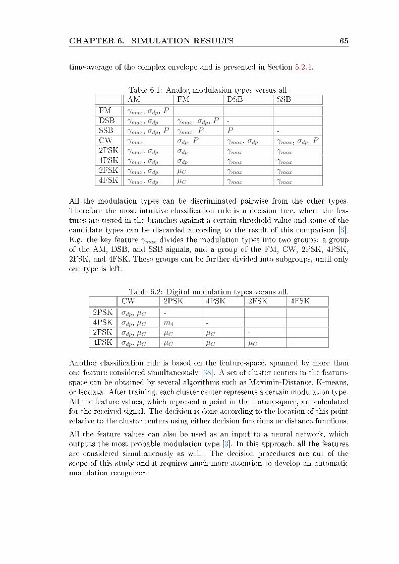
CHAPTER 6. SIMULATION RESULTS 65
time-average of the complex envelope and is presented in Section 5.2.4.
Table 6.1: Analog modulation types versus all.AM FM DSB SSB
FM γmax, σdp, P -DSB γmax, σdp γmax, σdp, P -SSB γmax, σdp, P γmax, P P -CW γmax σdp, P γmax, σdp γmax, σdp, P2PSK γmax, σdp σdp γmax γmax
4PSK γmax, σdp σdp γmax γmax
2FSK γmax, σdp µC γmax γmax
4FSK γmax, σdp µC γmax γmax
All the modulation types can be discriminated pairwise from the other types.Therefore the most intuitive classication rule is a decision tree, where the fea-tures are tested in the branches against a certain threshold value and some of thecandidate types can be discarded according to the result of this comparison [3].E.g. the key feature γmax divides the modulation types into two groups: a groupof the AM, DSB, and SSB signals, and a group of the FM, CW, 2PSK, 4PSK,2FSK, and 4FSK. These groups can be further divided into subgroups, until onlyone type is left.
Table 6.2: Digital modulation types versus all.CW 2PSK 4PSK 2FSK 4FSK
2PSK σdp, µC -4PSK σdp, µC m4 -2FSK σdp, µC µC µC -4FSK σdp, µC µC µC µC -
Another classication rule is based on the feature-space, spanned by more thanone feature considered simultaneously [38]. A set of cluster centers in the feature-space can be obtained by several algorithms such as Maximin-Distance, K-means,or Isodata. After training, each cluster center represents a certain modulation type.All the feature values, which represent a point in the feature-space, are calculatedfor the received signal. The decision is done according to the location of this pointrelative to the cluster centers using either decision functions or distance functions.All the feature values can also be used as an input to a neural network, whichoutputs the most probable modulation type [3]. In this approach, all the featuresare considered simultaneously as well. The decision procedures are out of thescope of this study and it requires much more attention to develop an automaticmodulation recognizer.
Chapter 7
Conclusions
In this study, several features for modulation classication were studied. Therelevant characteristics of the communication signals and statistical tools werepresented in the second and third chapters. A literature review of the previousmethods was carried out and the most promising methods were surveyed in moredetail. Further study of rst and second-order statistics including cyclostationarystatistics was done for digital modulated signals. During these derivations a novelfeature for the classication of the frequency shift keyed signals was found.The most interesting key features for pattern recognition purposes were selectedaccording to their applicability for the minimal signal representation and for theclassication of radio communication signals. The modulation types to be classiedwere selected emphasizing on these requirements. Therefore, the modulation typeswith a constant envelope and small symbol sets were used in the simulations. Atthe moment, an attractive application area would be software radio and otherrecongurable communication systems as real-time operating systems are beingdeveloped for signal processors. The pros and cons of the prospective featureswere discussed, as well.The discrimination performance of the potential features was studied by simula-tions with articially generated communication signals contaminated by additivewhite Gaussian noise. Also the robustness against noise was one of the criteriain the selection of the most interesting features. Simulations were carried out tostudy this behavior in dierent signal-to-noise ratio conditions. Also the inuenceof the sample set size was studied. The proposed feature showed very promisingresults in a zero-mean noise environment. It also has many desirable propertiesthat are required from reliable statistical estimates such as consistency.The cyclostationary statistics of the digital modulated signals might yield promis-ing features. In comparison to higher-order statistics, they possess some desirableproperties; e.g. lower variance. Due to their complicated appearance shown inthis study, the features derived in the cyclostationary context will need furtheranalysis. Also the inuence of dierent constellations on the classication of thephase shift keyed signals and its compensation would require more attention since

CHAPTER 7. CONCLUSIONS 67
the reviewed methods assume some xed constellation, which is not always thecase.The modulation recognition procedure would require, in addition to the featureextraction, a proper front-end and decision procedure. The task of the front-endwould be the channel equalization and to produce the correct sampled signal rep-resentation before feeding the measurements to the feature extraction system. Thedecision procedure takes the features as an input and outputs the most probablemodulation type which has produced the measured signal. As the front-end de-pends heavily on the application, the future work will concentrate on the decisionprocedures.
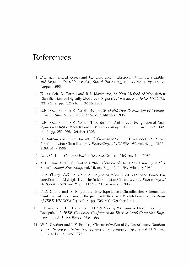
References
[1] P.O. Amblard, M. Gaeta and J.L. Lacoume, Statistics for Complex Variablesand Signals - Part II: Signals, Signal Processing, vol. 53, no. 1, pp. 1525,August 1996.
[2] K. Assaleh, K. Farrell and R.J. Mammone, A New Method of ModulationClassication for Digitally Modulated Signals, Proceedings of IEEE MILCOM'92, vol. 2, pp. 712716, October 1992.
[3] E.E. Azzouz and A.K. Nandi, Automatic Modulation Recognition of Commu-nication Signals, Kluwer Academic Publishers, 1996.
[4] E.E. Azzouz and A.K. Nandi, Procedure for Automatic Recognition of Ana-logue and Digital Modulations, IEE Proceedings Communication, vol. 143,no. 5, pp. 259266, October 1996.
[5] D. Boiteau and C. Le Martret, A General Maximum Likelihood Frameworkfor Modulation Classication, Proceedings of ICASSP '98, vol. 4, pp. 21652168, May 1998.
[6] A.B. Carlson, Communication Systems, 3rd ed., McGraw-Hill, 1986.
[7] Y.T. Chan and L.G. Gadbois, Identication of the Modulation Type of aSignal, Signal Processing, vol. 16, no. 2, pp. 149154, February 1989.
[8] K.M. Chugg, C-S. Long and A. Polydoros, Combined Likelihood Power Es-timation and Multiple Hypothesis Modulation Classication, Proceedings ofASILOMAR-29, vol. 2, pp. 11371141, November 1995.
[9] C-D. Chung and A. Polydoros, Envelope-Based Classication Schemes forContinuous-Phase Binary Frequency-Shift-Keyed Modulations, Proceedingsof IEEE MILCOM '94, vol. 3, pp. 796800, October 1994.
[10] I. Druckmann, E.I. Plotkin and M.N.S. Swamy, Automatic Modulation TypeRecognition, IEEE Canadian Conference on Electrical and Computer Engi-neering, vol. 1, pp. 6568, May 1998.
[11] W.A. Gardner and L.E. Franks, Characterization of Cyclostationary RandomSignal Processes, IEEE Transactions on Information Theory, vol. IT-21, no.1, pp. 414, January 1975.
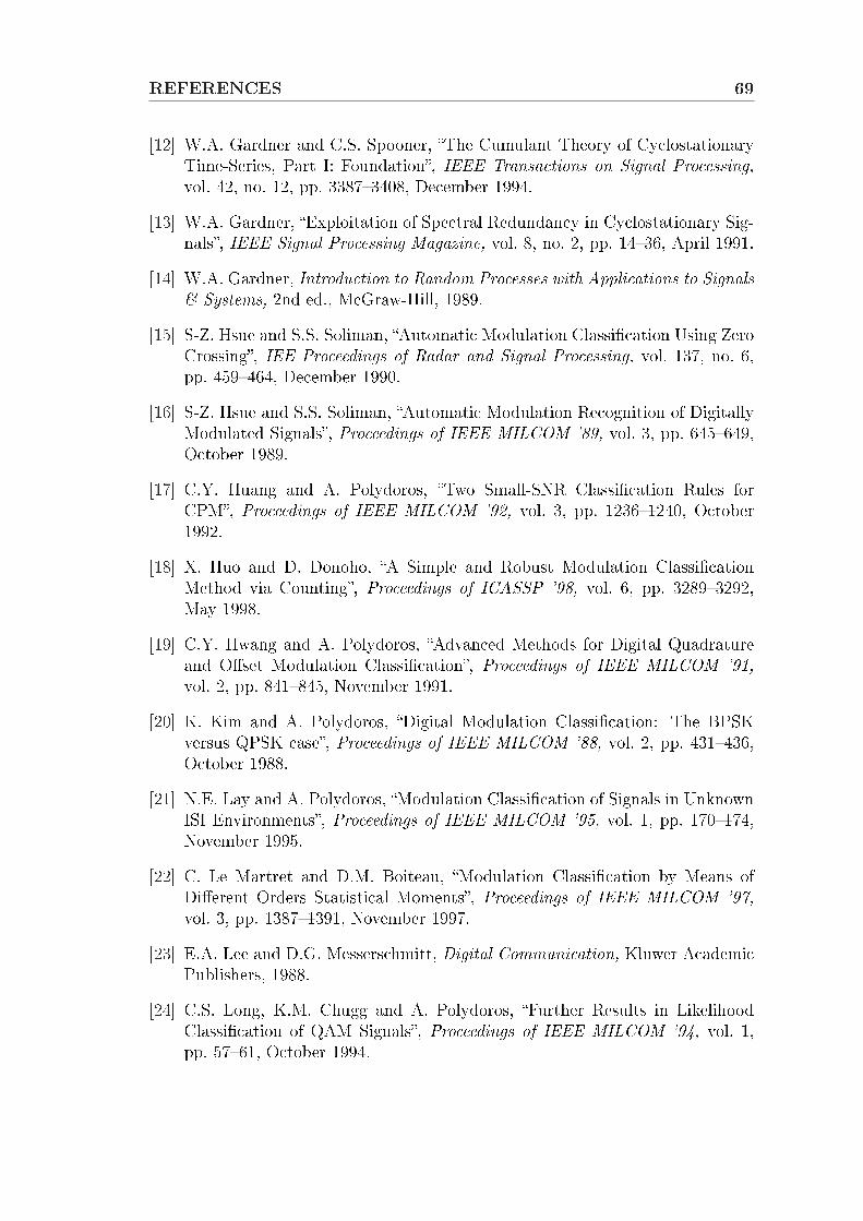
REFERENCES 69
[12] W.A. Gardner and C.S. Spooner, The Cumulant Theory of CyclostationaryTime-Series, Part I: Foundation, IEEE Transactions on Signal Processing,vol. 42, no. 12, pp. 33873408, December 1994.
[13] W.A. Gardner, Exploitation of Spectral Redundancy in Cyclostationary Sig-nals, IEEE Signal Processing Magazine, vol. 8, no. 2, pp. 1436, April 1991.
[14] W.A. Gardner, Introduction to Random Processes with Applications to Signals& Systems, 2nd ed., McGraw-Hill, 1989.
[15] S-Z. Hsue and S.S. Soliman, Automatic Modulation Classication Using ZeroCrossing, IEE Proceedings of Radar and Signal Processing, vol. 137, no. 6,pp. 459464, December 1990.
[16] S-Z. Hsue and S.S. Soliman, Automatic Modulation Recognition of DigitallyModulated Signals, Proceedings of IEEE MILCOM '89, vol. 3, pp. 645649,October 1989.
[17] C.Y. Huang and A. Polydoros, Two Small-SNR Classication Rules forCPM, Proceedings of IEEE MILCOM '92, vol. 3, pp. 12361240, October1992.
[18] X. Huo and D. Donoho, A Simple and Robust Modulation ClassicationMethod via Counting, Proceedings of ICASSP '98, vol. 6, pp. 32893292,May 1998.
[19] C.Y. Hwang and A. Polydoros, Advanced Methods for Digital Quadratureand Oset Modulation Classication, Proceedings of IEEE MILCOM '91,vol. 2, pp. 841845, November 1991.
[20] K. Kim and A. Polydoros, Digital Modulation Classication: The BPSKversus QPSK case, Proceedings of IEEE MILCOM '88, vol. 2, pp. 431436,October 1988.
[21] N.E. Lay and A. Polydoros, Modulation Classication of Signals in UnknownISI Environments, Proceedings of IEEE MILCOM '95, vol. 1, pp. 170174,November 1995.
[22] C. Le Martret and D.M. Boiteau, Modulation Classication by Means ofDierent Orders Statistical Moments, Proceedings of IEEE MILCOM '97,vol. 3, pp. 13871391, November 1997.
[23] E.A. Lee and D.G. Messerschmitt, Digital Communication, Kluwer AcademicPublishers, 1988.
[24] C.S. Long, K.M. Chugg and A. Polydoros, Further Results in LikelihoodClassication of QAM Signals, Proceedings of IEEE MILCOM '94, vol. 1,pp. 5761, October 1994.
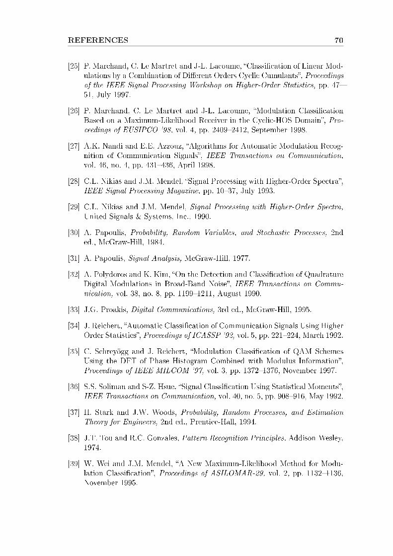
REFERENCES 70
[25] P. Marchand, C. Le Martret and J-L. Lacoume, Classication of Linear Mod-ulations by a Combination of Dierent Orders Cyclic Cumulants, Proceedingsof the IEEE Signal Processing Workshop on Higher-Order Statistics, pp. 4751, July 1997.
[26] P. Marchand, C. Le Martret and J-L. Lacoume, Modulation ClassicationBased on a Maximum-Likelihood Receiver in the Cyclic-HOS Domain, Pro-ceedings of EUSIPCO '98, vol. 4, pp. 24092412, September 1998.
[27] A.K. Nandi and E.E. Azzouz, Algorithms for Automatic Modulation Recog-nition of Communication Signals, IEEE Transactions on Communication,vol. 46, no. 4, pp. 431436, April 1998.
[28] C.L. Nikias and J.M. Mendel, Signal Processing with Higher-Order Spectra,IEEE Signal Processing Magazine, pp. 1037, July 1993.
[29] C.L. Nikias and J.M. Mendel, Signal Processing with Higher-Order Spectra,United Signals & Systems, Inc., 1990.
[30] A. Papoulis, Probability, Random Variables, and Stochastic Processes, 2nded., McGraw-Hill, 1984.
[31] A. Papoulis, Signal Analysis, McGraw-Hill, 1977.
[32] A. Polydoros and K. Kim, On the Detection and Classication of QuadratureDigital Modulations in Broad-Band Noise, IEEE Transactions on Commu-nication, vol. 38, no. 8, pp. 11991211, August 1990.
[33] J.G. Proakis, Digital Communications, 3rd ed., McGraw-Hill, 1995.
[34] J. Reichert, Automatic Classication of Communication Signals Using HigherOrder Statistics, Proceedings of ICASSP '92, vol. 5, pp. 221224, March 1992.
[35] C. Schreyögg and J. Reichert, Modulation Classication of QAM SchemesUsing the DFT of Phase Histogram Combined with Modulus Information,Proceedings of IEEE MILCOM '97, vol. 3, pp. 13721376, November 1997.
[36] S.S. Soliman and S-Z. Hsue, Signal Classication Using Statistical Moments,IEEE Transactions on Communication, vol. 40, no. 5, pp. 908916, May 1992.
[37] H. Stark and J.W. Woods, Probability, Random Processes, and EstimationTheory for Engineers, 2nd ed., Prentice-Hall, 1994.
[38] J.T. Tou and R.C. Gonzales, Pattern Recognition Principles, Addison-Wesley,1974.
[39] W. Wei and J.M. Mendel, A New Maximum-Likelihood Method for Modu-lation Classication, Proceedings of ASILOMAR-29, vol. 2, pp. 11321136,November 1995.
REFERENCES 71
[40] Y. Yang and C-H. Liu, An Asymptotic Optimal Algorithm for ModulationClassication, IEEE Communication Letters, vol. 2, no. 5, pp. 117119, May1998.
[41] Y. Yang and S.S. Soliman, Optimum Classier for M-ary PSK Signals, IEEEInternational Conference on Communications, vol. 3, pp. 16931697, June1991.
[42] Y. Yang and S.S. Soliman, Statistical Moments Based Classier for MPSKSignals, Proceedings of GLOBECOM '91, vol. 1, pp. 7276, December 1991.
[43] Y. Yang and S.S. Soliman, A Suboptimal Algorithm for Modulation Classi-cation, IEEE Transactions on Aerospace and Electronic Systems, vol. 33, no.1, pp. 3845, January 1997.
Appendix A
First and Second-Order Statistics ofDigital Modulated Signals
In this appendix, we derive the rst and second-order statistics and cyclic autocor-relations for digital modulated signals. The modulation types under considerationare M-ary amplitude, phase, and frequency shift keyed processes. Also the carrierwave process is dealt for consistency. The statistics are derived for continuous-timeprocesses with discrete symbol sequences. Oversampling with respect to symbolrate has to be used when the cyclic features are exploited with sampled sequences.The denition for the cyclic autocorrelation is presented in 3.1.2.In subsequent sections, we let M be the number and S[m] be an i.i.d randomsequence of the symbols with uniform probability mass function (PMF). Then wecan write
S[m] ∈ 0, 1, . . . , M − 1, M = 1, 2, 4, 8, . . . ,
P[S[m] = a
]=
1
M, a = 0, 1, . . . , M − 1, (A.1)
where m ∈ Z is the index of the mth symbol.
A.1 Carrier WaveThe complex envelope representation of the carrier wave (CW) process is C(t) =e0 = 1. The mean function and time-average is therefore trivially periodic µC(t) =µC(t + T ) = µC = 1 with any period T . The autocorrelation function is alsotrivially periodic RC(t1, t2) = RC(t1 + T, t2 + T ) = RC(t + τ
2, t − τ
2) = 1, where
τ = t1 − t2. The cyclic autocorrelation function can be expressed as
APPENDIX A. FIRST AND SECOND-ORDER STATISTICS OFDIGITAL MODULATED SIGNALS 73
RαC(τ) =
1
T
∫ ∞
−∞e−j2παtdt =
2π
Tδ(2πα), (A.2)
where the last identity follows from the Fourier transform pair 1 ↔ 2πδ(ω).
A.2 Amplitude Shift KeyingLet A[m] = 2S[m] + 1 − M , the complex envelope representation of the M-aryamplitude shift keying (MASK) process can be expressed as
C(t) =∞∑
m=−∞A[m]g(t−mT )
=∞∑
m=−∞
[2S[m] + 1−M
]g(t−mT ), (A.3)
where the distance between adjacent symbols is 2d = 2. The mean function of theMASK process can be expressed as
µC(t) = ES[C(t)] =∞∑
m=−∞
[2ES
[S[m]
]+ 1−M
]g(t−mT ) = 0, (A.4)
because
ES
[S[m]
]=
1
M[0 + 1 + · · ·+ (M − 1)] =
1
M
M(M − 1)
2=
M − 1
2, (A.5)
where we have used the identity for the sum of integers 1+2+3+ · · ·+n = n(n+1)2
.Thus the mean function and time-average of the MASK process is trivially periodicµC(t) = µC(t + T ) = µC = 0.The autocorrelation function of the MASK process can be expressed as
RC(t1, t2) = ES
[C(t1)C(t2)
]=
∞∑m=−∞
∞∑n=−∞
ES
[A[m]A[n]
]g(t1 −mT )g(t2 − nT )
=1
3(M2 − 1)
∞∑
k=−∞g(t1 − kT )g(t2 − kT ), (A.6)
APPENDIX A. FIRST AND SECOND-ORDER STATISTICS OFDIGITAL MODULATED SIGNALS 74
where the expectation ES
[A[m]A[n]
]can be expanded as
ES
[A[m]A[n]
]= ES
[(2S[m] + 1−M)(2S[n] + 1−M)
]= 4ES
[S[m]S[n]
]
+2ES
[S[m]
]+ 2ES
[S[n]
]− 2MES
[S[m]
]− 2MES
[S[n]
]
+M2 − 2M + 1, (A.7)
and the expectation ES
[S[m]S[n]
]for m 6= n, by Equation (A.5) and independent
symbols, can be expressed as
ES
[S[m]S[n]
]= ES
[S[m]
]ES
[S[n]
]=
(M − 1)2
4, (A.8)
and therefore Equation (A.7) is zero if m 6= n. The expectation ES
[S[m]S[n]
]for
m = n = k can be expressed as
ES
[S[m]S[n]
]= ES
[S2[k]
]=
1
M
[02 + 12 + · · ·+ (M − 1)2
]
=(M − 1)(2M − 1)
6, (A.9)
where we have used the identity for the sum of squared integers 12 +22 +32 + · · ·+n2 = n(n+1)(2n+1)
6. After some calculus, Equation (A.7) becomes
ES
[A[m]A[n]
]=
1
3(M2 − 1)δ(m− n). (A.10)
Thus the double summation in Equation (A.6) can be replaced by one summationover k = m = n. Let the signal pulse be a square g(t) = u(t)− u(t−mT ), whereT is the symbol duration. The autocorrelation function can now be expressed as
RC(t1, t2) =1
3(M2 − 1)
∞∑
k=−∞[u(t1 − kT )− u(t1 − (k + 1)T )][u(t2 − kT )
−u(t2 − (k + 1)T )] =
13(M2 − 1),
⌊t1T
⌋=
⌊t2T
⌋0, otherwise , (A.11)
where b·c denotes the integer part of the argument. The autocorrelation functionis invariant to a shift by T ; i.e. periodic. Thus the MASK process is wide-sensecyclostationary.
APPENDIX A. FIRST AND SECOND-ORDER STATISTICS OFDIGITAL MODULATED SIGNALS 75
By substitution τ = t1 − t2 and examination of the bounds of the products of theunit step functions, the autocorrelation function can be expressed as
RC(t +τ
2, t− τ
2) =
1
3(M2 − 1)
∞∑
k=−∞
[u(t− |τ |
2− kT )− u(t +
|τ |2− (k + 1)T )
]
×[u(τ + T )− u(τ − T )], (A.12)
where the last term of the product causes the autocorrelation to be zero when thelag is larger than T . Due to its periodicity, the autocorrelation function can beexpanded to its Fourier series and the coecients can be obtained as follows
RαC(τ) =
1
3T(M2 − 1)
∞∑
k=−∞
∫ ∞
−∞
[u(t− |τ |
2− kT )− u(t +
|τ |2− (m + 1)T )
]
×[u(τ + T )− u(τ − T )]e−j2παtdt (A.13)
=1
3T(M2 − 1)
∞∑
k=−∞
[(e−j2πα(
|τ |2
+kT ) − e−j2πα(−|τ |
2+(k+1)T )
) ∫ ∞
−∞u(t)e−j2παtdt
]
×[u(τ + T )− u(τ − T )] (A.14)
=1
3T(M2 − 1)
∞∑
k=−∞
(e−j2πα(
|τ |2
+kT ) − e−j2πα(− |τ |2
+(k+1)T ))( 1
j2πα+ πδ(2πα)
)
×[u(τ + T )− u(τ − T )], (A.15)
where α is the cyclic frequency, namely α = nT, n = 0,±1,±2, . . . , and n is the
number of harmonic. From Equation (A.14) we get Equation (A.15) by the time-shift property of Fourier transform f(t − τ) ↔ e−jωτF (ω) and Equation (A.15)follows from the Fourier transform of the unit step function u(t) ↔ 1
jω+ πδ(ω)
where ω = 2πf .
A.3 Phase Shift KeyingThe phase sequence for M-ary phase shift keying (MPSK) process can be expressedas Φ[m] = 2π
MS[m]. The complex envelope representation of the MPSK process will
be as follows
APPENDIX A. FIRST AND SECOND-ORDER STATISTICS OFDIGITAL MODULATED SIGNALS 76
C(t) =∞∑
m=−∞ejΦ[m]g(t−mT )
=∞∑
m=−∞ejΦ[m][u(t−mT )− u(t− (m + 1)T )], (A.16)
where the signal pulse is assumed to be a square g(t) = u(t)−u(t−T ). The meanfunction of C(t) can be expressed as
µC(t) = ES[C(t)] =∞∑
m=−∞ES[ejΦ[m]][u(t−mT )− u(t− (m + 1))] = 0,(A.17)
because
ES[ejΦ[m]] =1
Mej0 +
1
Mej 2π
M + · · ·+ 1
Mej(M−1) 2π
M
=1
M
[(e0 + ejπ) + (ej 2π
M + ej(M2
+1) 2πM ) + . . .
]= 0. (A.18)
Thus the mean function and time-average of the MPSK process is trivially periodicµC(t) = µC(t + T ) = µC = 0. The autocorrelation function of the MPSK processcan be expressed as
RC(t1, t2) = ES[C(t1)C(t2)] =∞∑
m=−∞
∞∑n=−∞
ES
[ej
[Φ[m]+Φ[n]
]](A.19)
×[u(t1 −mT )− u(t1 − (m + 1)T )][u(t2 − nT )− u(t2 − (n + 1)T )],
where due to the independent symbols, the expectation inside the summations form 6= n can be expressed as
ES
[ej
[Φ[m]+Φ[n]
]]= ES[ejΦ[m]]ES[ejΦ[n]] = 0, (A.20)
and for m = n = k
APPENDIX A. FIRST AND SECOND-ORDER STATISTICS OFDIGITAL MODULATED SIGNALS 77
ES
[ej
[Φ[m]+Φ[n]
]]= ES[ej2Φ[k]] =
1
M
[ej0 + ej 4π
M + · · ·+ ej(M−1) 4πM
]
=
1, M = 20, M = 4, 8, . . .
. (A.21)
When M = 4, 8, . . . , the autocorrelation function will be identically zero. For2PSK process, the expectation in Equation (A.21) is ES
[ej
[Φ[m]+Φ[n]
]]= δ(m−n).
Thus the summations over m and n can be replaced with one summation overk = m = n and Equation (A.20) becomes
RC(t1, t2) =∞∑
k=−∞[u(t1 − kT )− u(t1 − (k + 1)T )][u(t2 − kT )− u(t2 − (k + 1)T )]
=
1,
⌊t1T
⌋=
⌊t2T
⌋0, otherwise , (A.22)
where b·c denotes the integer part of the argument. Clearly RC(t1, t2) = RC(t1 +T, t2 + T ) and thus the 2PSK process is wide-sense cyclostationary. The autocor-relation function of the 2PSK process is identical to the autocorrelation functionof the MASK process except the constant 1
3(M2 − 1) which can be discarded due
to the linearity property of the Fourier transform. Thus the cyclic autocorrelationof the 2PSK process can be expressed as
RαC(τ) =
1
T
∞∑
k=−∞
(e−j2πα(
|τ |2
+kT ) − e−j2πα(−|τ |
2+(k+1)T )
)( 1
j2πα+ πδ(2πα)
)
×[u(τ + T )− u(τ − T )], (A.23)
where α is the cyclic frequency, namely α = nT, n = 0,±1,±2, . . . , and n is the
number of harmonic.
A.4 Frequency Shift KeyingThe complex envelope representation of the M-ary frequency shift keying (MFSK)process can be expressed as
APPENDIX A. FIRST AND SECOND-ORDER STATISTICS OFDIGITAL MODULATED SIGNALS 78
C(t) = expjω∆
∫ t ∞∑m=−∞
S[m]g(τ −mT )dτ
= expjω∆
∞∑m=−∞
S[m]
∫ t
[u(τ −mT )− u(τ − (m + 1)T )]dτ
= expjω∆
∞∑m=−∞
S[m](t−mT )[u(t−mT )− u(t− (m + 1)T )]
=∞∑
m=−∞ejω∆S[m](t−mT )[u(t−mT )− u(t− (m + 1)T )], (A.24)
where T is the symbol duration and the pulse shape is assumed to be a squareg(t) = u(t)− u(t−mT ). The expectation with respect to S[m] can be expressedas
µC(t) = ES[C(t)] =1
M
M−1∑a=0
∞∑m=−∞
ejω∆a(t−mT )[u(t−mT )− u(t− (m + 1)T )]
=[ 1
M+
1
M
M−1∑a=1
∞∑
k=−∞ejω∆a(t−kT )
][u(t + T − kT )− u(t + T − (k + 1)T )]
= µC(t + T ), (A.25)
where k = m + 1. Equation (A.25) shows that the mean function of the MFSKprocess is periodic and the time-average of the MFSK process is µC = 1
M.
The autocorrelation function of the MFSK process can be expressed as
RC(t1, t2) = ES[C(t1)C(t2)] =∞∑
m=−∞
∞∑n=−∞
ES[ejω∆[S[m](t1−mT )+S[n](t2−nT )]]
×[u(t1 −mT )− u(t1 − (m + 1)T )][u(t2 − nT )− u(t2 − (n + 1)T )]
=1
M
M−1∑a=0
∞∑
k=−∞ejω∆a(t1+t2−2kT )
×[u(t1 − kT )− u(t1 − (k + 1)T )][u(t2 − kT )− u(t2 − (k + 1)T )]
= RC(t1 + T, t2 + T ), (A.26)
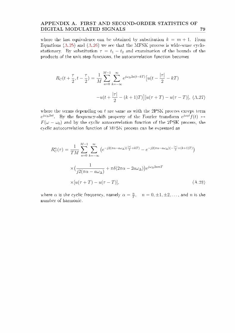
APPENDIX A. FIRST AND SECOND-ORDER STATISTICS OFDIGITAL MODULATED SIGNALS 79
where the last equivalence can be obtained by substitution k = m + 1. FromEquations (A.25) and (A.26) we see that the MFSK process is wide-sense cyclo-stationary. By substitution τ = t1 − t2 and examination of the bounds of theproducts of the unit step functions, the autocorrelation function becomes
RC(t +τ
2, t− τ
2) =
1
M
M−1∑a=0
∞∑
k=−∞ejω∆2a(t−kT )
[u(t− |τ |
2− kT )
−u(t +|τ |2− (k + 1)T )
][u(τ + T )− u(τ − T )], (A.27)
where the terms depending on t are same as with the 2PSK process except termejω∆2at. By the frequency-shift property of the Fourier transform ejω0tf(t) ↔F (ω − ω0) and by the cyclic autocorrelation function of the 2PSK process, thecyclic autocorrelation function of MFSK process can be expressed as
RαC(τ) =
1
TM
M−1∑a=0
∞∑
k=−∞
(e−j2(πα−aω∆)(
|τ |2
+kT ) − e−j2(πα−aω∆)(− |τ |2
+(k+1)T ))
×( 1
j2(πα− aω∆)+ πδ(2πα− 2aω∆)
)ejω∆2amT
×[u(τ + T )− u(τ − T )], (A.28)
where α is the cyclic frequency, namely α = nT, n = 0,±1,±2, . . . , and n is the
number of harmonic.