statistical handbook for assessing pig classification methods
132
Coordination: G´ erard DAUMAS Compilation: David CAUSEUR STATISTICAL HANDBOOK FOR ASSESSING PIG CLASSIFICATION METHODS: Recommendations from the “EUPIGCLASS” project group by CAUSEUR D., DAUMAS G., DHORNE T., ENGEL. B., FONT I FURNOLS M., HØJSGAARD S.
Transcript of statistical handbook for assessing pig classification methods
Coordination: Gerard DAUMASCompilation: David CAUSEUR
STATISTICAL HANDBOOKFOR ASSESSING
PIG CLASSIFICATIONMETHODS:
Recommendations fromthe “EUPIGCLASS” project group
by
CAUSEUR D., DAUMAS G., DHORNE T.,
ENGEL. B., FONT I FURNOLS M.,
HØJSGAARD S.


Collective of authors:
David CAUSEUR Universite de Bretagne-Sud,Laboratoire SABRES,Campus de Tohannic,Rue Yves Mainguy, 56000 Vannes,France.
Gerard DAUMAS Institut Technique du Porc,BP 35104, 35651 Le Rheu Cedex,France.
Thierry DHORNE Universite de Bretagne-Sud,Laboratoire SABRES,Campus de Tohannic,Rue Yves Mainguy, 56000 Vannes,France.
Bas ENGEL Animal Sciences Group,Wageningen UR, Lelystad.Address for correspondence:Biometris, PO Box 100, 6700 AC,Wageningen, The Netherlands.
Maria FONT I FURNOLS Institut de Recerca i TecnologiaAgroalimentaries IRTA-CTC,Granja Camps i Armet,17121 Monells (Girona), Spain.
Søren HØJSGAARD Danmarks JordbrugsForskningPB 50, 8830 Tjele, Denmark.
Acknowledgements:
This work is part of the EU project Growth “EUPIGCLASS”(GRD1-1999-10914) partly funded through the 5th Framework Pro-gramme, the Growth Generic Activity Measurement and Testing,and also partly through the Technological Development Programmefrom OFIVAL.
Many thanks are due to Rainer Nagel and Juan Alvarez from thePig and Poultry Office of the General Direction of Agriculture fortheir support and to Eli Olsen, from the Danish Meat Research In-stitute, for her excellent co-ordination of the EUPIGCLASS project.


FOREWORD
This publication is one of the outcomes of the Growth Project GRD1-1999-10914“EUPIGCLASS”. This project aimed for standardisation of pig carcass classifi-cation in the EU through improved statistical procedures and new technologicaldevelopments. It was co-ordinated by the Danish Meat Research Institute.
The project was divided into three workpackages. The objective of the workpackageII was to solve the main statistical problems encountered in the application ofthe EC regulations for pig classification, to anticipate future problems and toform a basis to update the regulations. This statistical handbook was thereforewritten to provide useful and detailed documentation to people responsible for thenational assessment of pig classification methods, both in the present and futureEU countries.
At the moment, this outcome of the EUPIGCLASS project has to be consideredas a working document that could be used in discussions about changes in theEU regulations for pig classification. Depending these changes (probably decidedupon in 2005), an update could be necessary before officially replacing the presentversion of the “Statistical Handbook for assessing pig classification methods” thatwas distributed at a EU Pigmeat Management Committee meeting in 2000.
This new version of the handbook offers a considerable improvement over the 2000version. The main proposal for an adaptation of the EC/2967/85 regulation isto replace the present error criterion “RMSE” by the “RMSEP”, that estimatesthe error of prediction and can be evaluated when Partial Least Squares (PLS) isused. The text is enhanced with many details and examples that will be of use toresearch workers and/or statisticians involved in pig classification.

Contents
Introduction 11
I Before the trial 21
1 Sampling with regard to a pig population 23
1.1 A short description of the population of interest . . . . . . . . . . 23
1.2 Sampling frame and some practical considerations . . . . . . . . . 26
1.2.1 Selection on line (last level) . . . . . . . . . . . . . . . . . 26
1.2.2 Selection of the slaughterhouses (second level) . . . . . . . 26
1.2.3 Selection of the regions (first level) . . . . . . . . . . . . . 27
1.3 Stratification . . . . . . . . . . . . . . . . . . . . . . . . . . . . . 27
2 Statistical Methods for creating Prediction Formulae 29
2.1 Introduction . . . . . . . . . . . . . . . . . . . . . . . . . . . . . . 29
2.1.1 OLS or rank reduced methods: a matter of dimensionality 30
2.1.2 An harmonized approach of the assessment of accuracy . . 30
2.2 Statistical Methods . . . . . . . . . . . . . . . . . . . . . . . . . . 31
2.2.1 The prediction model . . . . . . . . . . . . . . . . . . . . . 31
2.2.2 Estimation when the dimensionality is assumed to be known 32
2.2.3 Estimation of the dimensionality . . . . . . . . . . . . . . 35
2.2.4 Regression with structuring factors . . . . . . . . . . . . . 37
2.3 Validation . . . . . . . . . . . . . . . . . . . . . . . . . . . . . . . 38
2.3.1 MSE - The mean squared error . . . . . . . . . . . . . . . 38
2.3.2 MSEP – Using external data . . . . . . . . . . . . . . . . 38
2.3.3 Approximating MSEP by cross–validation . . . . . . . . . 39
2.3.4 Summary . . . . . . . . . . . . . . . . . . . . . . . . . . . 41
3 Sampling: selection on variables 43
3.1 The nature of the sample . . . . . . . . . . . . . . . . . . . . . . . 43
3.2 The size of the sample . . . . . . . . . . . . . . . . . . . . . . . . 45
3.3 The accuracy of the prediction formula . . . . . . . . . . . . . . . 46
7

4 Cost saving/precision increasing methods 494.1 The practical interest in these methods . . . . . . . . . . . . . . . 50
4.1.1 Reducing dissection cost . . . . . . . . . . . . . . . . . . . 504.1.2 Testing several instruments . . . . . . . . . . . . . . . . . 52
4.2 Double regression . . . . . . . . . . . . . . . . . . . . . . . . . . . 544.2.1 Introduction . . . . . . . . . . . . . . . . . . . . . . . . . . 544.2.2 Sampling . . . . . . . . . . . . . . . . . . . . . . . . . . . 554.2.3 Calculations . . . . . . . . . . . . . . . . . . . . . . . . . . 564.2.4 Required sample sizes n and N . . . . . . . . . . . . . . . 57
4.3 Two-phase updates based on reference predictors . . . . . . . . . 584.3.1 Creating the prediction formula . . . . . . . . . . . . . . . 594.3.2 Minimum costs sampling scheme . . . . . . . . . . . . . . 60
4.4 Validation issues . . . . . . . . . . . . . . . . . . . . . . . . . . . 61
5 Reporting to the Commission. Protocol for the trial 63
II During and after the trial 65
6 Some general comments on the management of the trial 67
7 Departures from the model (lack-of-fit) 71
8 Managing outliers 738.1 Aim . . . . . . . . . . . . . . . . . . . . . . . . . . . . . . . . . . 738.2 The issue . . . . . . . . . . . . . . . . . . . . . . . . . . . . . . . 738.3 Definitions . . . . . . . . . . . . . . . . . . . . . . . . . . . . . . . 748.4 Statistical solutions . . . . . . . . . . . . . . . . . . . . . . . . . . 75
8.4.1 Graphical studies . . . . . . . . . . . . . . . . . . . . . . . 758.4.2 Residuals analysis . . . . . . . . . . . . . . . . . . . . . . . 758.4.3 Influence analysis . . . . . . . . . . . . . . . . . . . . . . . 758.4.4 Robust estimation . . . . . . . . . . . . . . . . . . . . . . 76
8.5 Robust estimation . . . . . . . . . . . . . . . . . . . . . . . . . . . 768.5.1 Criteria . . . . . . . . . . . . . . . . . . . . . . . . . . . . 778.5.2 Efficiency . . . . . . . . . . . . . . . . . . . . . . . . . . . 788.5.3 Algorithm . . . . . . . . . . . . . . . . . . . . . . . . . . . 788.5.4 Protocol . . . . . . . . . . . . . . . . . . . . . . . . . . . . 78
9 Estimation and validation in practice. Examples 819.1 Available software . . . . . . . . . . . . . . . . . . . . . . . . . . . 819.2 A worked example . . . . . . . . . . . . . . . . . . . . . . . . . . 82
9.2.1 Description of data . . . . . . . . . . . . . . . . . . . . . . 829.2.2 Doing it in R/Splus . . . . . . . . . . . . . . . . . . . . . . 829.2.3 Doing it in SAS . . . . . . . . . . . . . . . . . . . . . . . . 93
9.3 Implementing cost saving methods . . . . . . . . . . . . . . . . . 1079.3.1 Double regression . . . . . . . . . . . . . . . . . . . . . . . 1079.3.2 Surrogate predictor regression . . . . . . . . . . . . . . . . 109
10 Prospects 11310.1 Non-linear regression . . . . . . . . . . . . . . . . . . . . . . . . . 11310.2 Variance functions . . . . . . . . . . . . . . . . . . . . . . . . . . 114
11 Reporting to the Commission - results of the trial 117
A References 119
B Technical details 123B.1 SAS Macros for PLS and PCR . . . . . . . . . . . . . . . . . . . . 123B.2 Genstat program for double-regression . . . . . . . . . . . . . . . 125B.3 Programs in R/Splus to select the best subset of predictors accord-
ing to the RMSEP . . . . . . . . . . . . . . . . . . . . . . . . . . 130B.4 Programs in R/Splus for double-sampling schemes . . . . . . . . . 131B.5 Logistic regression for dealing with sub-populations . . . . . . . . 132
9

Introduction
By Gerard Daumas
The main objective of this document is to help people dealing with pig clas-sification methods. The past and future extensions of the European Union makeharmonisation even more necessary. Previous research concerning the harmonisa-tion of methods for classification of pig carcasses in the Community has achievedto:
• the adoption of a simplified dissection method and therefore a new definitionof the lean meat percentage;
• the introduction of a sophisticated statistical method, called double regres-sion, as the “new standard”;
• amendments of regulations.
The present regulations are not easily understandable. It is therefore necessaryfor the new scientists dealing with this matter to obtain some interpretations.
In the past member states have chosen different ways for sampling and forparameters estimation. Anyway, two issues have appeared: the reduction of ex-perimental costs and the management of large sets of highly correlated variables.These difficulties have been solved by more complicated statistical methods butall deriving from classical linear regression which was the initial method in theEC regulation.
To cut the cost of one experimental trial, “double regression” has been firstintroduced in pig classification by Engel& Walstra (1991). To reduce the costs oftesting different instruments Daumas & Dhorne (1997) have introduced “regres-sion with surrogate predictors”. These methods fulfill the present EU require-ments and estimation of accuracy is available.
In parallel the Danes have first introduced PCR (Principal Component Re-gression) to test the Danish robot Classification Centre (10-20 variables) and thenPLS (Partial Least Squares) to test the Danish robot Autofom (more than 100variables). These methods are not explicitly authorized by the regulations as thecompulsory accuracy criteria is not available. It is therefore impossible to checkwether the EU requirements are fulfilled or not.
11
Introduction
A short discussion in the Pigmeat Management Committee about the trialsreports generally do not permit to judge such unusual and complicated methodsapplied in the scope of classification methods. It seems therefore useful to de-scribe in detail the new statistical methods used and to show how to check theconstraints of the regulations.
The first official version (draft 3.1) of this handbook has been distributed onFebruary 2000 to the member states delegates at a meeting of the Pigmeat Man-agement Committee. Contributions came from statisticians or meat scientistswho are national expert for pig classification.
The European research project (EUPIGCLASS) about standardisation of pigclassification methods, which involves all the contributors of the first version ofthe handbook, gives the means for a considerable improvement of the formerversion. Orienting more towards users, achieving a large consensus, increasingharmonisation between sections, going further into details and illustrating withexamples are the main ideas followed for writing up this new version. Neverthe-less, a central issue was how to estimate accuracy in PLS and how to harmonisethe calculation of this criteria in all the statistical methods.
At the same time, this project was an opportunity to make progress on oldproblems, sometimes discussed but never resolved, like for instance “representa-tive sample” and “outliers”.
This new version of the handbook is an outcome of EUPIGCLASS. It containsin particular some recommendations for changing the EU regulations. As thestatus of the handbook is a kind of complement to the EU regulations it meansthat an update will probably be necessary after having taken decisions in Brusselsconcerning the amendments to the regulations. In the case the discussions latea long time a first update based on the present EU regulations might be usefulduring the transitional period.
Then, at medium term other updates will depend on the progress in researchand technologies.
Basis for classification
A brief history
Pig classification is based on an objective estimation of the lean meat content ofthe carcass. As this criteria is destructive and very expensive to obtain, it hasto be predicted on slaughterline. The EC regulations contain some requirementson how to predict the reference. In order to ensure that the assessment resultsare comparable, presentation (carcass dressing), weight and lean meat contentof the carcass need to be accurately defined. These criteria were defined by thefollowing two regulations :
• Council Regulation (EEC) Nr 3320/84 of 13 November 1984 determining
12
Introduction
the Community scale for classification of pig carcasses;
• Commission Regulation (EEC) Nr 2967/85 of 24 October 1985 laying downdetailed rules for the application of the Community scale for classificationof pig carcasses.
These criteria have evolved leading to amendments of the regulations. Firstly,lean meat content was derived from dissection of all striated muscle tissue fromthe carcass as far as possible by knife. The carcass was defined by the bodyof a slaughtered pig, bled and eviscerated, whole or divided down the mid-line,without tongue, bristles, hooves and genital organs. As some other parts wereremoved on the slaughterlines of some Member States, the carcass was laterdefined (Commission Regulation 3513/93 of 14 December 1993) also withoutflare fat, kidneys and diaphragm.
However, full dissection, developed by the Institut fur Fleischerzeugung undVermarktung (in Kulmbach, Germany) and called “the Kulmbach reference me-thod”, is laborious and very time consuming (10 to 12 hours per half carcass andperson). In practice, several Member States used a national dissection methodinstead of the Kulmbach reference method, which was a source of biases.
In order to assess the extent of biases and to look for a more simplified dis-section method an EC wide trial was conducted in 1990/1991. The results ofthis trial were reported by Cook and Yates (1992). In this trial, a simplifieddissection method based on the dissection of four main parts (ham, loin, shoul-der and belly) was tested. Following discussions slight adaptations of the testedmethod were introduced. After large discussions about how to calculate the newlean meat content from the data of the new EU dissection method, a compromisewas found on the definition of this new criterion. The new lean meat contentand dissection method are briefly described by Commission Regulation (EEC)Nr 3127/94 of 20 December 1994 (amending 2967/85) and described in detail byWalstra and Merkus (1996). Though these new rules were immediately enforced,4 years later, in 1998, only 5 Member States had implemented them in theirslaughterhouses (Daumas and Dhorne, 1998). This very long transitional period,still not ended in 2003, results in new distorsions between Member States.
One reason for delaying the application of regulations could be the high costof a dissection trial. Though dissection time was halved, the new EU dissectionmethod is still time consuming (4-5 hours per half carcass and person).
Sources of errors
The present way of calculating the lean meat percentage is well documented(Walstra & Merkus, 1996). The formula involves both joints and tissues weights.The sources of errors come from the carcass dressing, the cutting, the dissectionand the weighting:
13

Introduction
• Definition of the carcass
Because of the high cost of dissection it was decided to dissect only one side(the left side). But in practice both sides are never identical, especially forsplitting difficulties. A specific difficulty concerns the head, which is notsplit on the slaughterlines in some countries. In this case the head shouldbe split to remove the brain. But this split generally provokes a largererror than dividing by 2 the head weight and then subtracting an inclusiveamount for a half brain (for instance 50 g).
The carcass weight used as the denominator of the lean meat percentage isdefined as the sum of all the joints regardless if they have to be dissected.This sum includes 12 joints.
• Jointing procedure
Jointing of the carcass originates from the German DLG-method (Scheperand Scholz, 1985). Extraction of the 4 main joints (ham, loin, shoulder andbelly) is a potential source of distorsions because of the lack of very preciseanatomical markers. Separation of all 4 joints is more or less problematic,but removing the shoulder is the main difficulty.
• Dissection procedure
Only the 4 main joints are dissected. The dissection involves a completetissue separation of each joint into muscle, bone and fat. Fat is dividedinto subcutaneous fat (including skin) and intermuscular fat. Remnants,such as glands, blood vessels and connective tissue loosely adhering to fat,are considered as intermuscular fat. Tendons and fasciae are not separatedfrom the muscles.
Some small difficulties concern:
→ designation of blood-soaked tissue to muscle or fat,
→ differentiation for some small parts between intermuscular fat and con-nective tissue (therefore weighed as muscle),
→ delimitation in some areas between subcutaneous fat and intermuscu-lar fat (but without consequence for lean meat percentage).
• Weighting
The present definition of muscle weight includes dissection and evaporationlosses. These losses are highly dependent on chilling conditions, tempera-ture, speed and quality of dissection. Moreover in some cases carcasses arenot dissected the day following slaughtering.
14
Introduction
At present, the specification only concerns the weighing accuracy. Allweights should be recorded at least to the nearest 10 g or to the nearest 5or 1 g, if possible.
The errors on the reference have been studied in WP1. Splitting and operatoreffect on jointing seem to be the most important.
Evolutions in the definition of the lean meat content
The lean meat percentage, hereafter denoted LMP, has always been defined as aratio between a muscle weight (MUS) and a joints weight (JOINTS), expressedin %: Y = 100 x C x MUS / JOINTS
When the full Kulmbach dissection was used all the joints were dissected. So,both MUS and JOINTS concerned the whole left side (C = 1).
When a simplified dissection was introduced, MUS refers to the 4 dissectedjoints while JOINTS still refers to the whole left. The nature of the ratio hastherefore changed because numerator and denominator do not refer to the samepiece of meat. Simultaneously, a scaling factor (”cosmetic”) was introduced inorder to maintain the same mean in the EU (C = 1.3). This is the presentdefinition in 2003.
EUPIGCLASS group recommends now to change the definition towards the% of muscle in the 4 main joints which means that numerator and denominatoragain will refer to the same piece of meat, but sticking with a simplified dissection.Then, a new scaling factor will be a point of discussion. A new value could bearound: C = 0.9 .
These changes on the response variable have an influence on the levels of theresidual variance and the prediction error.
Classification instruments
Equipments and variables
When Denmark, Ireland and the United Kingdom joined the Community in 1973,they argued that the measurements which they used - fat and muscle depthstaken by probe over the m. longissimus - were better predictors of leannessthan the criteria used in the common pig classification scheme of the originalsix member states - carcass weight, backfat measurements on the splitline anda visual assessment of conformation. Even so, these three countries themselvesused different instruments and probing positions.
Later on, the principles of the new EC scheme are agreed. To be accepteda method must use objective measurements and must be shown to be accurate.There is also some consistency in the methods used. Some member states usefat and muscle depths measured at similar points because trials have suggested
15
Introduction
that these tend to be good predictors. Several member states also use the sameinstruments with which to measure the fat and muscle depths, simply because thesame instruments are widely available throughout the EU and have been shownto be sufficiently accurate.
In the 80’s there was a desire to promote harmonisation of classification meth-ods within the Community, although each Member State had its own authorizedmethods. This could be achieved by all Member States using similar instruments,measuring at the same sites or using the same equations. Unfortunately the pigpopulations of Member States differ in their genetic history and there is concernthat they may differ in their leanness at the same subcutaneous fat and muscledepths. As expected, the results from the 1990 EC trial suggest there would be anoticeable loss in accuracy if a common prediction equation were imposed uponMember States (Cook & Yates, 1992).
The problem with standardisation of equipment is that it could provide onemanufacturer with a monopoly from which it would be difficult to change, andmight limit the incentive for developing more accurate or cheaper equipment.At present different Member States use a wide variety of equipment, ranging inprice and sophistication, from simple optical probes which are hand operatedand based on the periscope principle, to the Danish Autofom, a robotic systemcapable of automatically measure more than 2000 fat and muscle depths. Mostof the equipments can be seen on the website : www.eupigclass.org
The most common probes are based on an optical principle. Although handoperated, fat and muscle depths are automatically recorded. A light source nearthe top of the probe emits light and a receptor measures the reflection level, whichis different for fat and muscle tissues.
Some equipments use ultra-sounds also for measuring fat and muscle depths.Video-image analysis techniques are still under development. Other measure-
ments are used such as areas of fat and muscle tissues.In the future one can envisage the use of whole body scanners for example.
Documentation of measuring equipment
The need to consider precision arises from the fact that tests performed on pre-sumably identical materials under presumably identical circumstances do not, ingeneral, yield identical results. This is attributed to unavoidable random errors.
Various factors may contribute to the variability of results from a measure-ment method, including:
• the operator
• the equipment used
• the calibration of the equipment
16
Introduction
• the environment (temperature, humidity, etc.)
• the slaughter process
• the time elapsed between measurements
The use of statistical methods for measuring method validation is describedin ISO 5725. The use of the standard is well established in analytical chemistryfor instance (Feinberg, 1995). In the meat sector, DMRI have started to use theprinciples in the documentation of any measuring equipment (Olsen, 1997).
ISO 5725 In addition to a manual, the documentation must include a descrip-tion of the measuring properties. These are laid down on the basis of experimentswhich include all facets of the application of the instruments and should includethe following aspects:
AccuracyThe accuracy of the method includes trueness and precision. Trueness refers
to the agreement between the measuring result and an accepted reference value,and is normally expressed as the bias. The precision refers to the agreementbetween the measuring results divided into repeatability and reproducibility (seethe examples below). The two measures express the lowest and the highest vari-ation of the results and are indicated by the dispersions sr and sR. Finally thereliability of the method is relevantly defined as the ratio s2
D/(s2D + s2
R) wheresD indicates the natural variation of the characteristic. As a rule-of-thumb thereliability should be at least 80 % .
RobustnessIt is essential for the determination of accuracy that the sources of measuring
variations are known, and thereby a measure of the robustness of the methodtowards external factors. The influence of external factors (temperature, lightetc.) should be limited by determination of a tolerance field for these factors.
ReferenceIf the reference of the measuring method is another measuring method it
should be described by its precision. As far as possible certified reference mate-rials or measurements from accredited laboratories should be applied as absolutereferences.
Experiences from Danish tests
Repeatability of an automatic equipmentRepeatability is defined as the closeness of agreement between the results of
measurements on identical test material, where the measurements are carried outusing the same equipment within short intervals of time.
17
Introduction
The repeatability of Autofom has been tested by measuring some carcassestwice. When testing the repeatability of Autofom no formula for calculation oflean meat percentage on the basis of fat and muscle depth had been developed.Therefore, the “C measure”, which is the smallest fat depth at the loin in thearea of the last rib, was used as an expression of the Autofom measurements.The repeatability standard deviation was estimated at approximately 1 mm, asexpected.
Reproducibility of a manual equipmentNormally, reproducibility is defined as the closeness of agreement between the
results of measurements on an identical test material, where the measurementsare carried out under changing conditions.
Apart from random errors, the operators usually contribute the main partof the variability between measurements obtained under reproducibility condi-tions. When investigating the UNIFOM equipment the total error variancewas estimated at s2 ≈ 2.4 units and the contribution from the operators wass2operator ≈ 0.2units. As a consequence the average difference between two oper-
ators will be in the interval 0±1.96√
2s2operator or 0±1.1 units (95% confidence
limits).
Overview of the handbook
The first drafts of the statistical handbook were organized according the differ-ent statistical methods with the same plan for all chapters: model, estimation,validation. A first introductive chapter dealt with general statistical issues. Eachchapter has been written by a national expert of pig classification taking partto the meetings of the Pig Meat Management Committee in Brussels. The de-scription of the statistical methods were quite short and time was missing forintroducing examples.
For this new version it has been decided to completely modify the structure.As the main users of this handbook will be the national teams responsible ofassessing pig classification methods in their country a structure built from thepractical problems as they occur during the time appeared more suited. Giventhe dissection trial is the central point in such projects the handbook is split into2 main parts: before the trial and after the trial.
The described statistical methods are the same than in the former versionsbut notation has been harmonized, material has been thoroughly revised andextended, examples have been added and processed according the different soft-wares, the references have been updated throughout (Appendix A) and a report-writing section has been included. Furthermore, an attempt of harmonisationof the accuracy criteria has led for choosing the RMSEP. This new edition ex-plains therefore how to calculate it in all cases. For some specific cases formulae
18
Introduction
have been put in appendix B. The choice of a prediction error criteria has someinfluence on sampling. Sampling recommendations have therefore been adapted.
Part 1 deals mainly with sampling and the statistical methods for creatingprediction formulae. Sampling is split into two chapters, describing first somegeneral issues and then some specificities linked with the statistical method tobe used. For the description of the statistical methods it has been taken intoaccount the number of predictors (few vs. many) which is one of the charac-teristics of the classification instruments. The model underlying these 2 kind ofstatistical methods (multiple regression vs. PLS / PCR) is described for eachone. Then, estimation and validation are presented. A specific chapter describes2 methods used for saving experimental cost. Finally, the last chapter gives somerecommendations on what could be included in the protocol of the trial.
The second Part deals about what has to be done after the trial, i.e. dataprocessing and reporting. The main chapter consists of estimation and validationin practice. Some examples from pig classification support the different stagesof data processing which specificities are given for the main available software.Before that, an introductive chapter deals with the initial examination of datagiving in particular some recommendations on how to manage outliers and influ-ent data. The last chapter speaks about report-writing concerning the results ofthe trial which have to be presented in Brussels for gaining approval of the testedclassification methods.
The use of this handbook is quite easy. The reader has just a few questionsto answer :
• How many instruments to test: one or several ?
• Are there immediately available or not ?
• Do the instruments measure a few or many variables ?
• If many measurements what is the assumed dimensionality of the data ?
• Am I interested in saving experimental cost ?
• Which software may I use ?
According the answers the experimenter has just to read the concerned sec-tions.
19


Part I
Before the trial
21

Chapter 1
Sampling with regard to a pigpopulation
By Gerard Daumas
In Commission Regulation No 3127/94, Article 1, it is stated that a predictionformula should be based on “... a representative sample of the national or regionalpig meat production concerned by the assessment method ...”.
In statistics, sampling is the selection of individuals from a population ofinterest. Generally, in pig classification context the population of interest isdefined as the national population of slaughterpigs in a certain range of carcassweight.
A “representative sample” is an ambiguous concept. Generally, it is inter-preted as a sampling scheme with equal probabilities (uniform random sampling).Nevertheless, it is often more efficient to take units with unequal probabilities orto over-represent some fractions of the population (Tille, 2001). To estimate ac-curately a function of interest (here: a regression) one must look for informationin a wise way rather than to give the same importance to each unit.
We therefore interpret the EU regulation in the sense of a sample which aimsto assure valid and unbiased conclusions about the population.
Some basic knowledge about sampling can be obtained from basic text book,like for instance Cochran (1977).
1.1 A short description of the population of in-
terest
In the framework of EUPIGCLASS project a questionnaire about pig populationand classification was sent in 2001 to most of the EU member states and candidatecountries. Daumas (2003) reported a compilation of the answers. Below is theinformation relative to the heterogeneousness of the national populations.
23

Chapter 1. Sampling with regard to a pig population
“Subpopulations are an important issue for assessing classification methods.The questionnaire proposed the two main factors known having a significanteffect on the prediction of the lean meat proportion, i.e. sex and breed. OnlyItaly mentioned another kind of subpopulations: heavy pigs (110 - 155 kg) vs.light pigs (70 - 110 kg).
According to sex the slaughterpigs can have three sexual types: females, entiremales or castrated males (castrates). If evidently all countries slaughter females(around 50 % of the slaughtering) only three countries slaughter both entire andcastrated males in non-negligible proportions. Spain estimates to half and half theproportions of entire and castrated males while Denmark and Bulgaria announcethat around 10 % of the males are not castrated. Two countries slaughter onlyentire males: Great Britain and Ireland, but with a low slaughter weight (71 kg).All the other countries slaughter only castrates.
According to breeds the situation is more confused. In general, slaughter-pigs are not pure breeds but crosses between two, three or four breeds. Othersare synthetic lines developed by genetic companies. Generally no statistics areavailable on this matter. The answers are therefore to be considered as experts’estimations at a determined time. Some large countries, like Germany or GreatBritain, did not provide any piece of information. Some small countries, likeEstonia, may be considered as homogeneous.
All the other countries declared between two and four crossbreds, except theCzech Republic with six. The declared crossbred sum up to more than 90 % ofthe national slaughtering.
Crosses are mainly performed between the five following breeds : Large White(also called Yorkshire), Landrace, Pietrain, Hampshire and Duroc.”
24

Chapter 1. Sampling with regard to a pig population
Yea
r20
00P
ropor
tion
ofse
xual
types
(%)
Pro
por
tion
ofcr
ossb
reed
s(%
)Fem
ales
Cas
trat
esE
nti
rem
ales
Bre
ed1
Bre
ed2
Bre
ed3
Bre
ed4
Tot
al4
bre
eds
EU
countr
ies
Aust
ria
5050
6832
100
Bel
gium
54.5
450.
550
2020
595
Den
mar
k49
.346
.74.
050
3010
1010
0Fin
land
5049
1Fra
nce
5149
5525
1010
100
Ger
man
y50
50Ir
elan
d50
50It
aly
5050
9010
100
The
Net
her
lands
5050
6025
105
100
Spai
n50
2030
Sw
eden
4752
175
241
100
Unit
edK
ingd
.49
51C
andid
ate
c.B
ulg
aria
5046
440
4010
797
Cypru
s50
5070
1010
1010
0C
zech
Rep
ub.
5050
3228
139
81E
ston
ia50
50Pol
and
5050
Slo
vak
Rep
ub.
50.5
49.4
0.1
4530
205
100
Slo
venia
5050
Tab
le1.
1:P
ropor
tion
ofsu
bpop
ula
tion
s(s
exan
dbre
ed)
inth
eE
uro
pea
nco
untr
ies
25
Chapter 1. Sampling with regard to a pig population
1.2 Sampling frame and some practical consid-
erations
National pig populations are so wide that no sampling frame is available. It is atechnical barrier for a random sampling.
As it is not possible to directly select the pigs it is therefore needed to selectfirst intermediary units (either pig farms or slaughterhouses). In practice, as theclassification measurements (predictors) are taken on slaughterline, it is oftenmore convenient to select slaughterhouses rather than pig farms. This kind ofsampling plan is called a “two-level sampling plan” (Tille, 2001). At each levelany plan may be applied.
1.2.1 Selection on line (last level)
If there is no stratification, a kind of systematic sampling can be performed. Asystematic sampling is the selection of every kth element of a sequence. Using thisprocedure, each element in the population has a known and equal probability ofselection. This makes systematic sampling functionally similar to simple randomsampling. It is however, much more efficient and much less expensive to do.
The researcher must ensure that the chosen sampling interval does not hidea pattern. Any pattern would threaten randomness. In our case care has to betaken about batches which correspond to pig producers. Batches size is variable.It may be judicious for instance to select no more than one carcass per producer(eventually a maximum of two).
1.2.2 Selection of the slaughterhouses (second level)
In most countries there are several ten slaughterhouses. But because of practicalconsiderations, especially regarding dissection, it would be difficult to select ran-domly the slaughterhouses. Furthermore, it is generally not an important factorstructuring the variability. Slaughter and cooling process are much less importantthan the origin of the pigs. In all cases the selection of the slaughterhouses hasto be reasoned.
If the national population is considered as homogeneous then the slaughter-houses selection has no great influence. Nevertheless, higher is the number ofslaughterhouses higher is the sample variability.
In some countries the differences between slaughterhouses mainly come fromthe different proportions of slaughterpigs genotypes. When these differences aremarked and the proportions in the national population are known a stratifiedsampling (see section 1.1) is suited. Then, higher is the number of slaughterhouseshigher is the variability within genotypes. After having chosen a certain numberof slaughterhouses and taking into account the proportions of genotypes in each
26

Chapter 1. Sampling with regard to a pig population
slaughterhouse it can be deduced the proportions of each genotype in the totalsample that has to be taken in each slaughterhouse.
1.2.3 Selection of the regions (first level)
In some other countries where regional differences are marked, due for instanceto genotype, feeding, housing, a kind of stratification (see section 1.1) may beperformed on regions when statistical data are available. Then, one or more“regionally representative slaughterhouses” have to be selected within regions.We therefore have a “3-level plan” (regions, slaughterhouses, pigs).
1.3 Stratification
Stratification is one of the best ways to introduce auxiliary information in asampling plan in order to increase the accuracy of parameters. Here, the auxiliaryinformation corresponds to the factor(s) of heterogeneousness (like sex and breed)of the national population.
If a population can be divided into homogeneous subpopulations, a smallsimple random sampling can be drawn from each, resulting in a sample that is“representative” of the population. The subpopulations are called strata. Thesampling design is called stratified random sampling.
In the literature many factors influencing the corporal composition have beenreported. Among those having the most important effects on the lean meatpercentage itself and on its prediction sex and genotype may be identified in adissection trial.
Significant differences between sexes were reported for instance in the EU byCook and Yates (1992), in The Netherlands by Engel and Walstra (1991b, 1993),in France by Daumas et al. (1994) and in Spain by Gispert et al. (1996).
Most EC member states considered their pig population to be geneticallyheterogeneous, with up to six genetic subpopulations (see section 1.1). Most ofthe European slaughterpigs come from crosses between three or four breeds. Themain difference is generally due to the boar (sire line), which gives more or lesslean content in the different selection programmes. High differences are expectedfor instance between Pietrain and Large White boars. This effect is reduced aftercrosses with the sow (mother line). Nevertheless, in some countries the genotypemay have an important effect. In that case the national population cannot beconsidered as homogeneous and a stratified random sampling is therefore moreefficient than a simple random sampling (i.e., same sample size gives greaterprecision).
Then two cases have to be considered:
• the stratification factor is not used as predictor in the model,
27
Chapter 1. Sampling with regard to a pig population
• the stratification factor is also used as predictor in the model,
The first case could be a good way for managing the genotypes. An optimumallocation (or disproportionate allocation) is the best solution when estimates ofthe variability are available for each genotype. Each stratum is proportionateto the standard deviation of the distribution of the variable. Larger samples aretaken in the strata with the greatest variability to generate the least possiblesampling variance. The optimal allocation depends on the function of interest:here a regression. Note that to infer a single equation to population one mustre-weight the carcasses within stratum (here: genotype) proportional to share ofpopulation.
If no (reliable) information is available on the intra stratum variability then aproportional allocation can be performed. Proportionate allocation uses a sam-pling fraction in each of the strata that is proportional to that of the total pop-ulation.
The second case (see also section 2.2.4) could be for instance a way for man-aging the sex. As sex is known on slaughterline and easy to record then sex canbe put in the model of prediction of the lean meat proportion. Following the con-clusions of the 1990 EC trial (Cook and Yates, 1992), France decided to introduceseparate equations for the sexual types when sex effect is significant (Daumas etal., 1998). In that case it does not matter if sampling is proportionate or dispro-portionate. Nevertheless, as the standard deviation is higher for castrates thanfor females it is more efficient to select a higher proportion of castrates (Daumasand Dhorne, 1995).
A very specific case is the Dutch situation where sex was used both in themodel and for stratification (Engel and Walstra, 1993). Unlike France, sex is notrecorded on slaughterline in The Netherlands. So, they decided to use a non-linear model for predicting the sex through a logistic regression (see AppendixB5). As sex is predicted in this two-stage procedure the gain in accuracy is muchlower than for separate formulas. Moreover, if the allocation would have beenoptimal it would have been necessary to re-weight samples (proportional to shareof population) to infer to population.
28
Chapter 2
Statistical Methods for creatingPrediction Formulae
By David Causeur, Gerard Daumas, Bas Engel and Søren Højs-gaard.
2.1 Introduction
In pig carcass classification, the LMP of a carcass is predicted from of a set ofmeasurements made on the carcass. These measurements (explanatory variables)can be e.g. ultrasound or, as is the case for the data used in the illustrative workedexample, measurements of physical characteristics and thicknesses of fat andmeat layer at different locations. In practice, a prediction formula is establishedby applying statistical methods to training data (data for which not only theexplanatory variables but also the true LMP is known from e.g. dissection).
Different statistical methods are currently used in the European Union toassess the prediction formulae. The choice for a particular prediction method de-pends mostly on the instrument which is used to measure the predictors. Theseinstruments can indeed roughly be classified into two groups: the probes measur-ing a small number of predictors at few specific locations in the carcass, and otherinstruments extracting many measurements by a more general scanning of thecarcass. In the former case, the explanatory variables are usually highly corre-lated. Consequently, a classical statistical method such as ordinary least squares(OLS) may be inappropriate for constructing the prediction formula because thepredictions can have very large variances. Therefore one often use alternativemethods, and two such are partial least squares (PLS) or principal componentregression (PCR), see Sundberg (1999) for discussion of this.
29
Chapter 2. Statistical Methods for creating Prediction Formulae
2.1.1 OLS or rank reduced methods: a matter of dimen-sionality
The first issue the user is faced with is naturally the choice between OLS andan alternative method. This problem is generally addressed in the statisticalhandbooks by somewhat theoretical arguments which claim for instance thatPLS has always to be be preferred first because it is known to be at least as goodas PCR and second because OLS is nothing more than a particular case of PLS.Also it must be true, we will try in the following to give more insight to the choiceof a particular method in the specific context of pigs classification.
First, in this context, the practitioners can observe that the prediction for-mulae assessed with few predictors, usually less than 5, and those assessed withhundreds of predictors are almost as accurate, or at least that the difference inaccuracy is not proportional to the difference between the numbers of predictorsthat are measured. This shall points out that the amounts of predicting infor-mation collected in both cases are not so different. Furthermore, whatever theinstrument that is used, it appears in all cases that a small number of axis ofpredicting information can be identified, or equivalently, that only a small num-ber of latent variables are indirectly measured. This number of latent variablesis often referred as the dimensionality of the instrumental predictors.
Usually, the most important latent variable can be seen as the fat content inthe carcass. The second latent variable characterizes the amount of lean meatand the third one is related to the physical conformation of the carcass. To bemore complete, each of the former latent variables can sometimes be doubledto distinguish between fat or lean contents that could be due either to geneticsor to feeding. Finally, as a first approximation and only on the basis of whathas already been observed in the past experiments, it can be said that about 6axis of predicting information can at most be expected to be identified in pigcarcass data. Consequently, the use of rank reduced method can actually berecommended when the number of instrumental predictors is very large relativeto this dimensionality. In the other situations, it seems to be reasonable to inspectcarefully the redundancy of the predicting information and even to compare thepredictive ability of OLS and PLS.
2.1.2 An harmonized approach of the assessment of accu-racy
Harmoniously assessing the accuracy of the prediction formulae is currently oneof the objectives of the EC-regulations that frame pigs classification in the Eu-ropean Union. Although these regulations still contain some ambiguity withrespect to their practical applications, they tend to ensure a minimum level ofaccuracy by restrictions on the sample size and the estimated residual standarddeviation. However, they do not yet account for substantial differences between
30
Chapter 2. Statistical Methods for creating Prediction Formulae
the prediction methods. As it will be mentioned thereafter, in the case of highlycorrelated predictors, PLS and PCR often work well in practice being superiorto OLS in terms of accuracy of the predictions. This is basically achieved byallowing for bias in the estimation of the regression coefficients in order to reduceits variance. Due to this bias, the estimated residual standard deviation doesprobably not reflect faithfully the predictive ability of PLS and PCR. Moreover,these methods suffer from other deficiencies. First, they are defined iterativelymeaning that precise interpretation is difficult to grasp. Second, the statisticalproperties are difficult to stipulate. To be specific, it is unclear how to estimatethe residual variance and how to estimate variance of the parameter estimators.
The will for harmonization obviously appeals for the choice of a single cri-terion that first can be computed whatever the prediction method and second,that reflects the predictive ability rather than the precision of estimation. Inthe following sections, it is advised to choose the Root Mean Squared Error ofPrediction, designed by RMSEP, computed by a full cross-validation techniqueand some arguments motivating this choice are given.
2.2 Statistical Methods
Our purpose here is to give technical hints to actually calculate the predictionformulae. Further details on this kind of issues can be found in many handbooksdedicated to statistical models for prediction, for instance Rao and Toutenburg(1999). These estimation procedures are sometimes presented as if the dimen-sionality was not part of the estimation issue. However, in most of the practicalsituations of pigs classification, an important and sensitive work is done on thedata either to define a relevant set of predictors before the prediction formulais assessed or to investigate the dimensionality problem. In other words, thedimensionality is actually a meta-parameter, which estimation has to be consid-ered in that section and at least accounted for when the problem of validatingthe prediction formulae will be addressed. For that reason, first in the case theset of predictors and the dimensionality are assumed to be known, we presentthe usual procedures that underly the prediction packages generally provided bythe softwares. Then the estimation of the dimensionality or the selection of arelevant set of predictors is investigated and specific recommendations are given.Hereafter, the validation problem is considered with respect both to the fittingprocedure itself and to the selection step.
2.2.1 The prediction model
It is supposed that the LMP, generically denoted by y, is measured together withthe p predictors x = (x1, . . . , xp) on n sampled carcasses. The training datathat are used to establish the prediction formula are therefore D = {(yi, xi), i =
31
Chapter 2. Statistical Methods for creating Prediction Formulae
1, . . . , n}. Further details about sampling are mentioned in chapter 3. Up tosophistications that could be shown to be relevant in some special cases, thefollowing linear regression model is traditionally assumed:
yi = β0 + β1xi1 + . . . + βpxip + εi,
where εi ∼ N(0, σ) stands for the residual error, β0 denotes the offset and β =(β1, . . . , βp)
′ is the p−vector of the slope coefficients.Therefore, the general expression for the prediction formulae is a linear com-
bination of the instrumental predictors:
y(x) = β0 + β1x1 + . . . + βpxp
where y(x) denotes the predicted LMP for a carcass which values for the instru-mental predictors are x, β0 is the estimated offset and βj, j = 1, . . . , p, are theestimated slope coefficients.
Up to now, call β = (β1, . . . , βp)′ the p− vector of the estimated slopes.
2.2.2 Estimation when the dimensionality is assumed tobe known
The least-squares criterion
Estimation usually consists in minimizing a criterion that measures the globaldifference between predicted and observed values. For theoretical reasons thatgo beyond the scope of our purpose, the least-squares criterion appears to berelevant, at least in some extent:
SS(β0, β) =n∑
i=1
(yi − β0 − β1xi1 + . . . + βpxip)2.
It will be shown in section 8 that alternative criteria can be used especially ifoutliers are suspected to influence abnormally the estimation procedure.
The OLS solution
Minimization of this criterion can be achieved by equating its derivativesrelative to each coefficient: for all j = 0, 1, . . . , p, ∂SS
∂βj(β0, β) = 0. Therefore, β0
and β are obtained by solving what is called the system of normal equations:
∂SS∂β0
(β0, β) = −2∑n
i=1(yi − β0 − β1xi1 + . . . + βpxip) = 0,∂SS∂β1
(β0, β) = −2∑n
i=1 xi1(yi − β0 − β1xi1 + . . . + βpxip) = 0,∂SS∂β2
(β0, β) = −2∑n
i=1 xi2(yi − β0 − β1xi1 + . . . + βpxip) = 0,...
......
......
∂SS∂βp
(β0, β) = −2∑n
i=1 xip(yi − β0 − β1xi1 + . . . + βpxip) = 0.
32
Chapter 2. Statistical Methods for creating Prediction Formulae
The first equation states that the predicted value for the LMP when the valuesof the instrumental predictors are the mean values xj is simply the average leanmeat y or in other words:
β0 = y − β1x1 − . . .− βpxp.
Imputing this value of the offset in the p other equations yields:
∑ni=1(xi1 − x1)
([yi − y]− β1 [xi1 − x1] + . . . + βp [xip − xp]
)= 0,∑n
i=1(xi2 − x2)([yi − y]− β1 [xi1 − x1] + . . . + βp [xip − xp]
)= 0,
......
...∑ni=1(xip − xp)
([yi − y]− β1 [xi1 − x1] + . . . + βp [xip − xp]
)= 0.
,
or equivalently, with matrix notations:
sxy − Sxxβ = 0,
where sxy and Sxx denote respectively the empirical covariance p−vector betweeny and the predictors and the p × p empirical variance-covariance of the instru-mental predictors.
At that point, it has to be noted that solving this equation is just a matter ofregularity of Sxx. In the very convenient case where Sxx is not ill-conditioned, inother words when exhibiting the inverse matrix S−1
xx is not subject to numericalproblems, solving the least-squares problem leads to the OLS solution:
βOLS = S−1xx sxy.
It is well-known that the former OLS estimator has desirable properties suchas unbiasedness and an easy-to-compute variance, which makes inference, andespecially prediction, easier.
Biased solutions
Ill-conditioned matrices Sxx are known to be encountered when the predict-ing information is redundant, or equivalently when the number of predictors ismuch higher than the dimensionality. In that case, some methods, called biasedregression methods, consist in replacing S−1
xx by an approximate version, denotedby G:
βBR = Gsxy.
This modification of the OLS estimator makes the new estimator biased. In thatcase, the mean squared error MSE is traditionally used to reflect more properlythe accuracy of the estimator:
MSE = bias2 + variance.
33
Chapter 2. Statistical Methods for creating Prediction Formulae
The most relevant choices for G aim at a compensation of the increase of the biasby a reduction of the variance. Globally, this trade-off between bias and variancecan even lead to a better accuracy in terms of mean squared error.
Many techniques can be used to find a satisfactory G matrix and some ofthem are generally provided by the statistical softwares. Maybe the most intuitivetechnique is the ridge regression that consists in choosing G in a family of matricesindexed by a single value λ:
G ∈ Gλ ={(Sxx + λIp)
−1, λ > 0}
.
In this approach, the trade-off between bias and variance is transposed into a kindof cursor λ that can be moved from zero to introduce bias and simultaneouslyreduce the variance.
Rank-reduced solutions
Other techniques, sometimes said to be rank-reduced, are getting more andmore popular since they directly connect the choice of G with the problem ofdimensionality. Two of the most widely spread among these methods are PCRand PLS. The first idea behind these methods is the extraction from the predictorsof a small number, say k, of independent new variables tj = (t1j, t2j, . . . , tnj)
′
defined as linear combinations of the centered instrumental predictors:
tij = w1j(xi1 − x1) + w2j(xi2 − x2) + wpj(xip − xip),
where wj = (w1j, w2j, . . . , wpj)′ is called the jth vector of loadings. To bridge the
gap with the introductory words on dimensionality, the extracted componentsmake it concrete the latent variables and therefore k can be interpreted as thedimensionality. For brevity, call X the n× p matrix of the centered values of theinstrumental predictors, T the n×k matrix of the components values and W thep× k matrix of loadings, then:
T = XW.
In both cases of PCR and PLS, the extraction of the components can be presentedfrom an algorithmic point of view as an iterative procedure. In the case ofPCR, this extraction procedure is simply a Principal Component Analysis of theinstrumental predictors: initially, t1 is the component with maximal variance,then t2 is chosen as the component with maximal variance among those with nullcovariance with t1, and so on until the kth component. In the case of PLS, thestrategy differs only by the criterion which is optimized at each step: the varianceis indeed replaced by the squared covariance with the response. This differenceis often used as an argument to underline the superiority of PLS relative to PCRin a context of prediction: extraction of the PLS components is indeed oriented
34
Chapter 2. Statistical Methods for creating Prediction Formulae
towards prediction whereas extraction of the PCR components does not rely onthe values of the response at all.
Once the components are extracted, the second phase consists in predictingthe response by OLS as if the predictors were the components. The n−vector offitted values of the response by the rank-reduced methods is therefore obtainedas follows:
y = T (T ′T )−1T ′Y,
= X W (W ′SxxW )−1W ′sxY︸ ︷︷ ︸ˆβRR
.
Therefore, in the case of rank-reduced methods, the vector of estimated slopecoefficients is given by:
βRR = W (W ′SxxW )−1W ′sxY .
Equivalently, the generic expression for the G matrix figuring an approximationof S−1
xx is expressed as follows:
G = W (W ′SxxW )−1W ′.
The algorithms providing the matrices of loadings in the case of PLS and PCRhave been described above. In the particular case of PCR, this algorithm yieldsin some sense the best approximation of Sxx by a matrix G−1 with rank k.
Now, in the case of PLS, Helland (1998) showed that the iterative algorithmconsists finally in choosing the most relevant G, leading to the smallest MSE, inthe following set of matrices:
G ∈ Gk,α ={α0Ip + α1Sxx + . . . + αkS
kxx, α = (α0, α1, . . . , αk)
′.}
,
which also makes the PLS estimator optimal in some sense.Although the problem of dimensionality may be considered by some prac-
titioners as an additional trouble specific to rank-reduced methods, it must benoted that this problem is of course only masked while using OLS. It is indeedvery tempting to build regression models with all the present predictors to im-prove the fit but it must be kept in mind that this conservative behavior damagesthe predictive ability of the prediction formula. This issue is addressed in thenext section and recommendations are given to estimate properly the dimensionmeta-parameter.
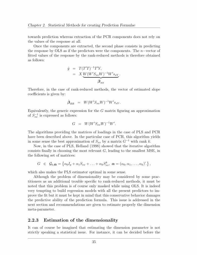
2.2.3 Estimation of the dimensionality
It can of course be imagined that estimating the dimension parameter is notstrictly speaking a statistical issue. For instance, it can be decided before the
35
Chapter 2. Statistical Methods for creating Prediction Formulae
regression experiment that, say three, pre-chosen instrumental predictors will besufficient to predict the LMP. In that case, provided that this choice is relevant,it can be considered that the dimensionality equals the number of predictors andOLS can simply be performed in the old-fashioned way to derive the predictionformula. Suppose now that hundreds of instrumental predictors are collected bya general scanning of the carcass, but that a prior reliable knowledge availableon these instrumental predictors makes it relevant to consider that only, saythree, latent variables are measured. In that case as well, setting the dimensionparameter to three is also possible without further statistical developments.
However, due to an uncertainty about the redundancy in the predicting infor-mation that is collected, a statistical procedure is sometimes needed to chose for aproper value for the dimension parameter. Note that the redundancy analysis canat first be approached by widely spread exploratory data tools, such as PrincipalComponents Analysis (PCA), that enable a simplified reading of a large correla-tion matrix. However, these tools do not generally allow for a rigorous analysisof the redundancy within the instrumental predictors in our context of predictionsince they do not enable a proper display of the partial dependencies between theresponse and some predictors conditionally on others. Therefore, we recommendan exhaustive comparison of the predictive abilities that can be obtained for eachvalue of the dimension parameter. Note that this strategy supposes that a val-idation criterion that quantifies the predictive ability of a prediction method ispreviously defined: this issue is discussed below in section 2.3 and the Root MeanSquared Error of Prediction (RMSEP) is recommended as a validation criterion.
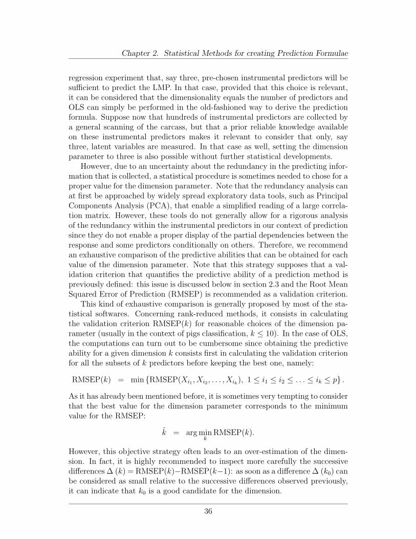
This kind of exhaustive comparison is generally proposed by most of the sta-tistical softwares. Concerning rank-reduced methods, it consists in calculatingthe validation criterion RMSEP(k) for reasonable choices of the dimension pa-rameter (usually in the context of pigs classification, k ≤ 10). In the case of OLS,the computations can turn out to be cumbersome since obtaining the predictiveability for a given dimension k consists first in calculating the validation criterionfor all the subsets of k predictors before keeping the best one, namely:
RMSEP(k) = min {RMSEP(Xi1 , Xi2 , . . . , Xik), 1 ≤ i1 ≤ i2 ≤ . . . ≤ ik ≤ p} .
As it has already been mentioned before, it is sometimes very tempting to considerthat the best value for the dimension parameter corresponds to the minimumvalue for the RMSEP:
k = arg mink
RMSEP(k).
However, this objective strategy often leads to an over-estimation of the dimen-sion. In fact, it is highly recommended to inspect more carefully the successivedifferences ∆ (k) = RMSEP(k)−RMSEP(k−1): as soon as a difference ∆ (k0) canbe considered as small relative to the successive differences observed previously,it can indicate that k0 is a good candidate for the dimension.
36
Chapter 2. Statistical Methods for creating Prediction Formulae
The estimation procedures presented before are illustrated by the analysis ofa real data set in section 9.2.
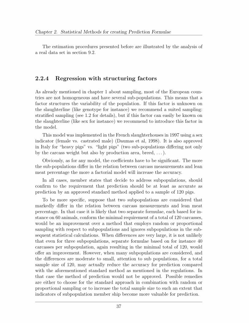
2.2.4 Regression with structuring factors
As already mentioned in chapter 1 about sampling, most of the European coun-tries are not homogeneous and have several sub-populations. This means that afactor structures the variability of the population. If this factor is unknown onthe slaughterline (like genotype for instance) we recommend a suited sampling:stratified sampling (see 1.2 for details), but if this factor can easily be known onthe slaughterline (like sex for instance) we recommend to introduce this factor inthe model.
This model was implemented in the French slaughterhouses in 1997 using a sexindicator (female vs. castrated male) (Daumas et al, 1998). It is also approvedin Italy for “heavy pigs” vs. “light pigs” (two sub-populations differing not onlyby the carcass weight but also by production area, breed, . . . ).
Obviously, as for any model, the coefficients have to be significant. The morethe sub-populations differ in the relation between carcass measurements and leanmeat percentage the more a factorial model will increase the accuracy.
In all cases, member states that decide to address subpopulations, shouldconfirm to the requirement that prediction should be at least as accurate asprediction by an approved standard method applied to a sample of 120 pigs.
To be more specific, suppose that two subpopulations are considered thatmarkedly differ in the relation between carcass measurements and lean meatpercentage. In that case it is likely that two separate formulae, each based for in-stance on 60 animals, conform the minimal requirement of a total of 120 carcasses,would be an improvement over a method that employs random or proportionalsampling with respect to subpopulations and ignores subpopulations in the sub-sequent statistical calculations. When differences are very large, it is not unlikelythat even for three subpopulations, separate formulae based on for instance 40carcasses per subpopulation, again resulting in the minimal total of 120, wouldoffer an improvement. However, when many subpopulations are considered, andthe differences are moderate to small, attention to sub populations, for a totalsample size of 120, may actually reduce the accuracy for prediction comparedwith the aforementioned standard method as mentioned in the regulations. Inthat case the method of prediction would not be approved. Possible remediesare either to choose for the standard approach in combination with random orproportional sampling or to increase the total sample size to such an extent thatindicators of subpopulation member ship become more valuable for prediction.
37
Chapter 2. Statistical Methods for creating Prediction Formulae
2.3 Validation
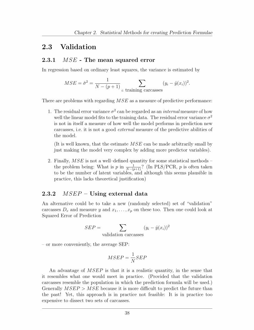
2.3.1 MSE - The mean squared error
In regression based on ordinary least squares, the variance is estimated by
MSE = σ2 =1
N − (p + 1)
∑i: training carcasses
(yi − y(xi))2.
There are problems with regarding MSE as a measure of predictive performance:
1. The residual error variance σ2 can be regarded as an internal measure of howwell the linear model fits to the training data. The residual error variance σ2
is not in itself a measure of how well the model performs in prediction newcarcasses, i.e. it is not a good external measure of the predictive abilities ofthe model.
(It is well known, that the estimate MSE can be made arbitrarily small byjust making the model very complex by adding more predictor variables).
2. Finally, MSE is not a well–defined quantity for some statistical methods –the problem being: What is p in 1
N−(p+1)? (In PLS/PCR, p is often taken
to be the number of latent variables, and although this seems plausible inpractice, this lacks theoretical justification)
2.3.2 MSEP – Using external data
An alternative could be to take a new (randomly selected) set of “validation”carcasses Dv and measure y and x1, . . . , xp on these too. Then one could look atSquared Error of Prediction
SEP =∑
validation carcasses
(yi − y(xi))2
– or more conveniently, the average SEP:
MSEP =1
NSEP
An advantage of MSEP is that it is a realistic quantity, in the sense thatit resembles what one would meet in practice. (Provided that the validationcarcasses resemble the population in which the prediction formula will be used.)Generally MSEP > MSE because it is more difficult to predict the future thanthe past! Yet, this approach is in practice not feasible: It is in practice tooexpensive to dissect two sets of carcasses.
38
Chapter 2. Statistical Methods for creating Prediction Formulae
2.3.3 Approximating MSEP by cross–validation
An alternative to having an external validation data set Dv as discussed above isto use cross–validation methods: Here we suggest the use of leave–one–out crossvalidation, as it is easy to implement in practice:
This works as follows: For each carcass i
1. Delete the ith carcass from the training set:
2. Estimate β0, β1, . . . , βp from the remaining observations
3. Predict y for the ith carcass and calculate
SEP−i = (yi − y−i(xi))2
where y−1(x) is the predictor obtained when the ith carcass is excludedfrom the data set before estimating the regression parameters.
Next, calculate the PREdiction Sum of Squares PRESS =∑
i SEP−i andthe average PRESS APRESS = 1
NPRESS.
How much difference does it make in practice?
The question is now: How similar are APRESS and MSEP in practice? To providesome insight to this question we consider the Danish carcass classification data,see Section 9.2.
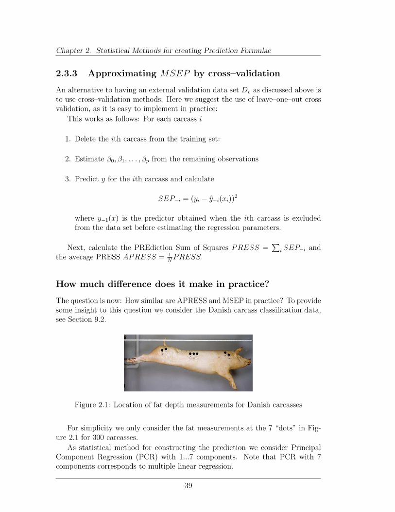
Figure 2.1: Location of fat depth measurements for Danish carcasses
For simplicity we only consider the fat measurements at the 7 “dots” in Fig-ure 2.1 for 300 carcasses.
As statistical method for constructing the prediction we consider PrincipalComponent Regression (PCR) with 1...7 components. Note that PCR with 7components corresponds to multiple linear regression.
39
Chapter 2. Statistical Methods for creating Prediction Formulae
Design of study
The study was made as follows: Split data in two:
• N = 120, N = 60 and N = 30 training carcasses
• M = 150 validation carcasses
Then we calculate RMSE =√
1N
SE, (an internal measure of precision),
RMSEP =√
1M
SEP , (the “truth”), and RAPRESS =√
1N
PRESS (a cross-
validation quantity, which should be close to the “truth”)
Results
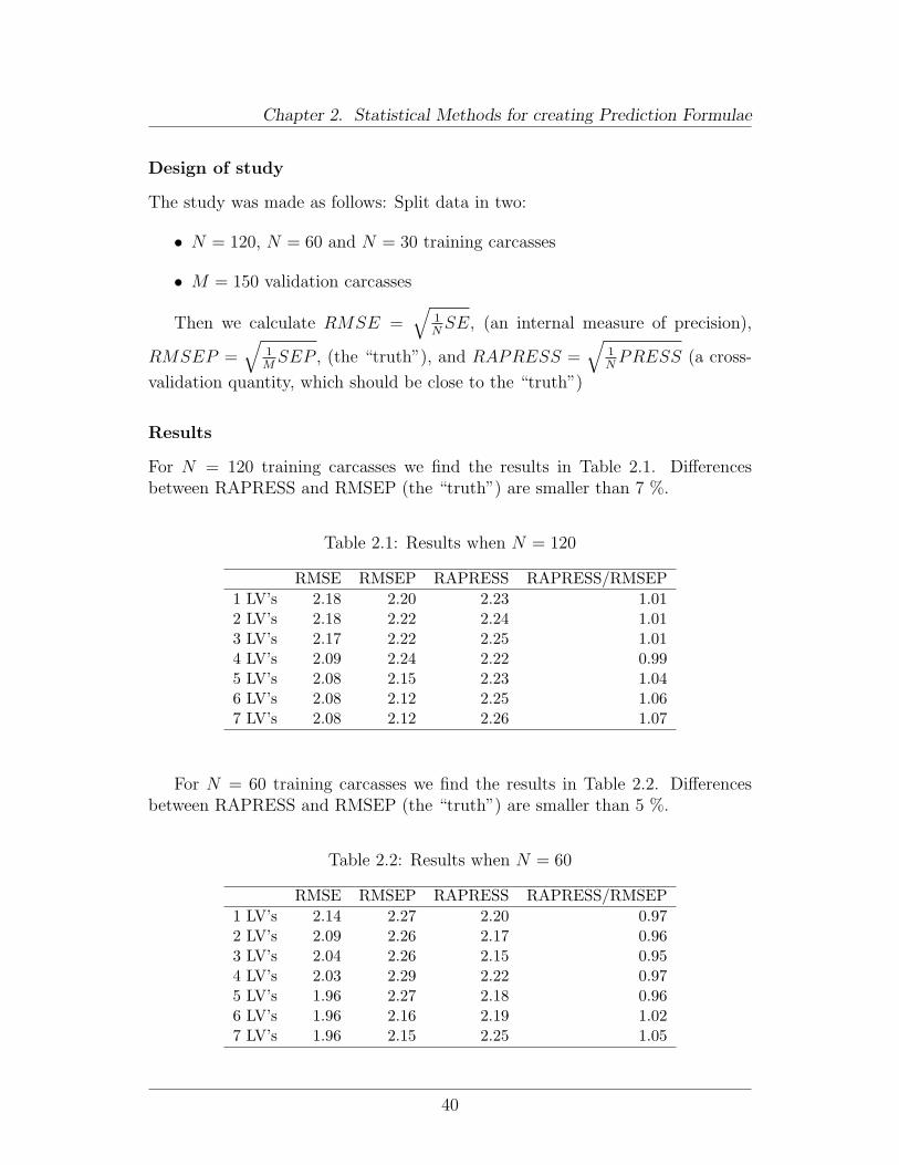
For N = 120 training carcasses we find the results in Table 2.1. Differencesbetween RAPRESS and RMSEP (the “truth”) are smaller than 7 %.
Table 2.1: Results when N = 120
RMSE RMSEP RAPRESS RAPRESS/RMSEP1 LV’s 2.18 2.20 2.23 1.012 LV’s 2.18 2.22 2.24 1.013 LV’s 2.17 2.22 2.25 1.014 LV’s 2.09 2.24 2.22 0.995 LV’s 2.08 2.15 2.23 1.046 LV’s 2.08 2.12 2.25 1.067 LV’s 2.08 2.12 2.26 1.07
For N = 60 training carcasses we find the results in Table 2.2. Differencesbetween RAPRESS and RMSEP (the “truth”) are smaller than 5 %.
Table 2.2: Results when N = 60
RMSE RMSEP RAPRESS RAPRESS/RMSEP1 LV’s 2.14 2.27 2.20 0.972 LV’s 2.09 2.26 2.17 0.963 LV’s 2.04 2.26 2.15 0.954 LV’s 2.03 2.29 2.22 0.975 LV’s 1.96 2.27 2.18 0.966 LV’s 1.96 2.16 2.19 1.027 LV’s 1.96 2.15 2.25 1.05
40
Chapter 2. Statistical Methods for creating Prediction Formulae
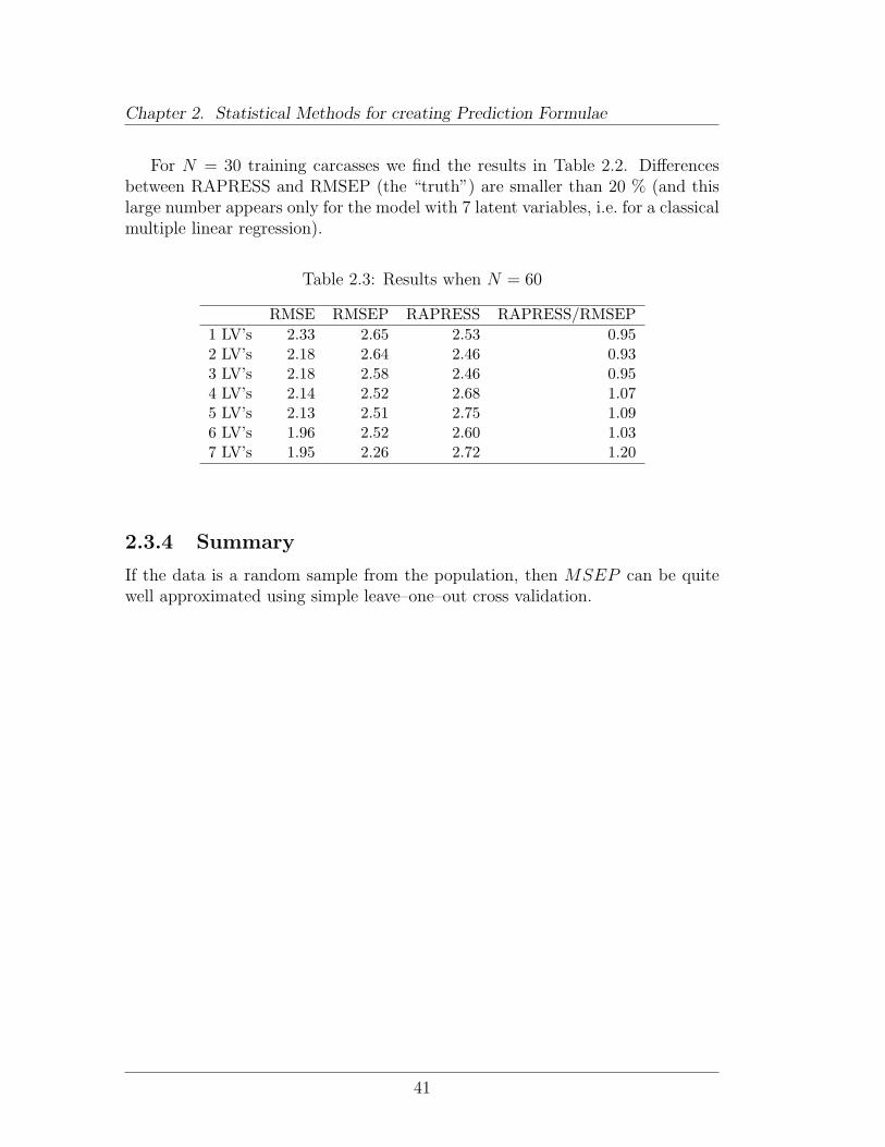
For N = 30 training carcasses we find the results in Table 2.2. Differencesbetween RAPRESS and RMSEP (the “truth”) are smaller than 20 % (and thislarge number appears only for the model with 7 latent variables, i.e. for a classicalmultiple linear regression).
Table 2.3: Results when N = 60
RMSE RMSEP RAPRESS RAPRESS/RMSEP1 LV’s 2.33 2.65 2.53 0.952 LV’s 2.18 2.64 2.46 0.933 LV’s 2.18 2.58 2.46 0.954 LV’s 2.14 2.52 2.68 1.075 LV’s 2.13 2.51 2.75 1.096 LV’s 1.96 2.52 2.60 1.037 LV’s 1.95 2.26 2.72 1.20
2.3.4 Summary
If the data is a random sample from the population, then MSEP can be quitewell approximated using simple leave–one–out cross validation.
41

Chapter 3
Sampling: selection on variables
By Bas Engel
3.1 The nature of the sample
In Commission Regulation No 3127/94, Article 1, it is stated that a predictionformula should be based on “...a representative sample of the national or regionalpig meat production concerned by the assessment method ...”.
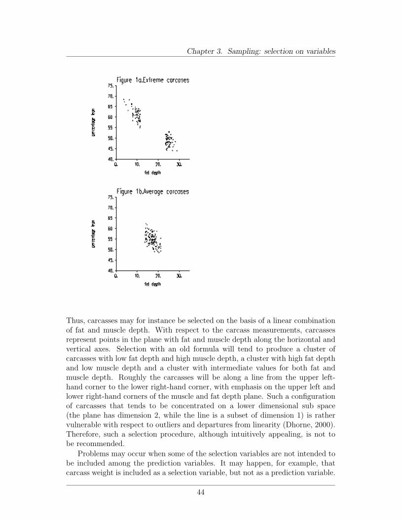
To be considered representative, samples do not need to be chosen completelyat random. In fact, because we focus on the variation in y given the value of x inLR, statistical theory allows us to select the carcasses on the basis of x. This canbe profitable, because selection of carcasses with more extreme fat or muscle depthmeasurements will improve the accuracy of the estimated values β0 and β1 forconstant β0 and coefficient β1 and thus improve the accuracy of prediction. Thisis illustrated in Figure 1, where the standard errors of the estimates β0 and β1 areconsiderably smaller for selection of carcasses with extreme x-values comparedto selection of carcasses with moderate x-values. Consequently, carcasses fordissection are often not selected randomly but according to a sampling schemethat favors a larger percentage of more extreme instrumental measurements. Ofcourse carcass values should not be too extreme, in other to avoid selection ofcarcasses of abnormal animals. Also, in practise sampling scheme (a) in Figure 1is usually supplemented with carcasses with moderate x-values as well, otherwisedepartures from linearity can hardly be detected. Curvature may lead to poorpredictions for moderate x-values.
A common sampling scheme in carcass classification is the 40-20-40 % scheme.Suppose that µx and σx are the mean and standard deviation for x in the popu-lation. In the 40-20-40 % scheme, 40 % of the sample is selected such that valuesof x are below µx − σx, 40 % is above µx + σx and 20 % is in between.
Carcasses may be selected on the basis of an ”old” prediction formula, whenthat formula is based on the same or similar instrumental carcass measurements.
43
Chapter 3. Sampling: selection on variables
Thus, carcasses may for instance be selected on the basis of a linear combinationof fat and muscle depth. With respect to the carcass measurements, carcassesrepresent points in the plane with fat and muscle depth along the horizontal andvertical axes. Selection with an old formula will tend to produce a cluster ofcarcasses with low fat depth and high muscle depth, a cluster with high fat depthand low muscle depth and a cluster with intermediate values for both fat andmuscle depth. Roughly the carcasses will be along a line from the upper left-hand corner to the lower right-hand corner, with emphasis on the upper left andlower right-hand corners of the muscle and fat depth plane. Such a configurationof carcasses that tends to be concentrated on a lower dimensional sub space(the plane has dimension 2, while the line is a subset of dimension 1) is rathervulnerable with respect to outliers and departures from linearity (Dhorne, 2000).Therefore, such a selection procedure, although intuitively appealing, is not tobe recommended.
Problems may occur when some of the selection variables are not intended tobe included among the prediction variables. It may happen, for example, thatcarcass weight is included as a selection variable, but not as a prediction variable.
44
Chapter 3. Sampling: selection on variables
This is a common phenomenon among many past proposals. Such a samplingprocedure is not covered by standard LR theory. For standard theory to apply,all selection variables have to be included as prediction variables as well. Such apotentially faulty combination of selection and LR may have direct consequencesfor authorization of a carcass measurement instrument (Engel et al., 2003). Wewill return to this particular problem later on.
3.2 The size of the sample
In ordinary linear regression, intercept β0 and slope β1 are estimated by themethod of least squares, i.e. estimates ˆbeta0 and β1 minimize the sum of squareddeviations:
n∑i=1
(yi − β0 − β1xi)2
Denoting the minimum value by RSS (residual sum of squares), an estimate forthe variance σ2 is:
s2 = RSS/d.
The degrees of freedom d in the numerator are equal to the sample size n reducedby the number p of unknowns to be estimated in the formula:
d = n− p.
For example, with one prediction variable x, we have two unknowns β0 and β1, sop = 2 and for a sample of n = 120 we have d = 120−2 = 118 degrees of freedom.Somewhat confusingly both the (unknown) population standard error σ and itsestimate s are often referred to as the residual standard deviation (RSD).
The accuracy of estimators β0 and β1 is reflected by their associated stan-dard errors. Each of these standard errors is a multiple of σ2, say c0σ
2/√
n andc0σ
2/√
n. Constants c0 and c1 depend on the configuration of x-values. Roughly:the more widely separated the values of x, the smaller these constants will be.With increasing sample size, the standard errors decrease with order 1/
√n.
The minimum required sample size for LR in the EC regulations is fixedin Article 1 of Commission Regulation No 3127/97 at n = 120. Each procedureproposed should be as accurate as LR based on a sample of n = 120 carcasses. Anexample of an alternative procedure to LR that we mentioned before is double-regression (DR). DR is based on a double-sampling procedure. Carcasses aredissected by a relatively quick and cheap national dissection method and only partof these carcasses are also dissected by the more time consuming and expensiveEC-reference method. The two dissection procedures may be applied to the same
45
Chapter 3. Sampling: selection on variables
or to different carcass halves of the same carcass. DR is specifically mentionedin Article 1 of Commission Regulation No 3127/97. The number of carcasses nwhich are (also) dissected according to the EC reference method should at leastequal 50. The total number of carcasses N , all dissected by the quick nationalmethod, should be high enough such that the precision is at least as high as LRfor 120 EC-reference dissections. In Engel & Walstra (1991a) it is shown howlarge the sample sizes N and N should be for DR to be as precise as LR for120 EC-reference dissections. Engel & Walstra (1991a) present accurate largesample results that avoid complete distributional assumptions. More accuratesmall sample results, assuming normality, are presented in Causeur and Dhorne(1998).
3.3 The accuracy of the prediction formula
The accuracy of prediction depends on the accuracy of estimates β0 and β1, butalso on the size of the error components ε. The accuracy of β0 and β1, as followsfrom the discussion so far, depends on the sample size and on the configuration ofx-values. The size of the error terms ε is quantified by the residual variance σ2. Itis important to realize that the selection of carcasses does affect the accuracy ofβ0 and β1, but not the accuracy of s2 as an estimator for σ2. The accuracy of s2
is measured by its standard error. Under a linear regression model this standarderror is equal to σ2
√2/d, where d is the degrees of freedom. Since d = n−p and n
is at least 120 and with LR p will be relatively small, say smaller than 6, roughlythe standard error of s2 decreases with order 1/
√n. By choosing larger samples
and appropriate configurations of x-values, we can make sure that β0 + β1 ∗ x isas close to β0 + β1 ∗ x as we want it to be. In fact with a sample size of 120 thedifference between a random sample and a sample of selected carcasses is fairlysmall (Engel et al., 2003; Font I Furnols,2002). However, we cannot reduce thecontribution to the prediction error of the error terms ε, as quantified by theresidual variance σ2. The size of σ2 depends on the measurement instrumentand the pig population. Unless some of the instrumental measurements thatwere initially not used, perhaps for practical reasons, are added to the equationlater on, there is no possibility to reduce σ2. Similar comments can be madewith respect to a cost saving method such as DR, where we estimate the samecoefficients β0 and β1 as in ordinary LR, but in a more efficient way. Hence,with DR we can attain a high accuracy for the estimates β0 and β1, but we haveto deal with the same residual variance σ2 as in LR. This implies that σ is thecrucial quantity for authorization of an instrument. It is therefore very importantto form a correct impression of the size of σ. When, due to an inept samplingprocedure, s does not offer an accurate impression of σ, this can have unfortunateconsequences for authorization. This may happen when some of the variables thatare included for selection are not included in the prediction formula. For details
46

Chapter 3. Sampling: selection on variables
we refer to Engel et al. (2003).
47

Chapter 4
Cost saving/precision increasingmethods
By David Causeur, Gerard Daumas, Thierry Dhorne and Bas Engel
In the previous chapters, some aspects of the interactions between the sta-tistical recommendations that are expected from this handbook and the require-ments laid down by the EC-regulations have been dealt with. Some of theserequirements (EC, 1994a and 1994b) are aiming to ensure a minimum level ofaccuracy by restrictions on the methodology used to establish the prediction for-mula. Roughly speaking, unreliability of the prediction formulæ is expected tobe avoided or at least reduced by a minimum sample size (currently 120 refer-ence dissections) and a maximum limit for a validation criterion (currently 2.5for the Residual Standard Deviation). As the reference dissections are heavilytime-consuming, an indirect consequence of the EC-requirements is the need forexpensive regression experiments. This chapter is devoted to the presentation ofstatistical methods that can be used to face that problem of experimental costs, orequivalently to save experimental units in the framework of the EC-requirements.
Some countries have chosen indeed to adopt new statistical methodologieswhich account for both the experimental cost and the EC-requirements in thedefinition of the sampling scheme. Basically, these new methods consist in re-placing reference dissection by cheaper approximated versions for some of thesampled carcasses. Section 4.1 is devoted to a further investigation of the prac-tical advantages of such a novelty.
As it is explained in details by Engel and Walstra (1991a and 1991b) orCauseur and Dhorne (1998), the subsequent sampling scheme involves two sam-ples: a first one for which reference dissections and approximate reference dissec-tions are performed together with measurements of the predictors and a secondone where only cheaper dissections are performed. Table 4.1 displays the gen-eral form of the two-phase sampling schemes. Minimum costs strategies are thenobtained by relevant choices of the sample sizes. More detailed explanations are
49
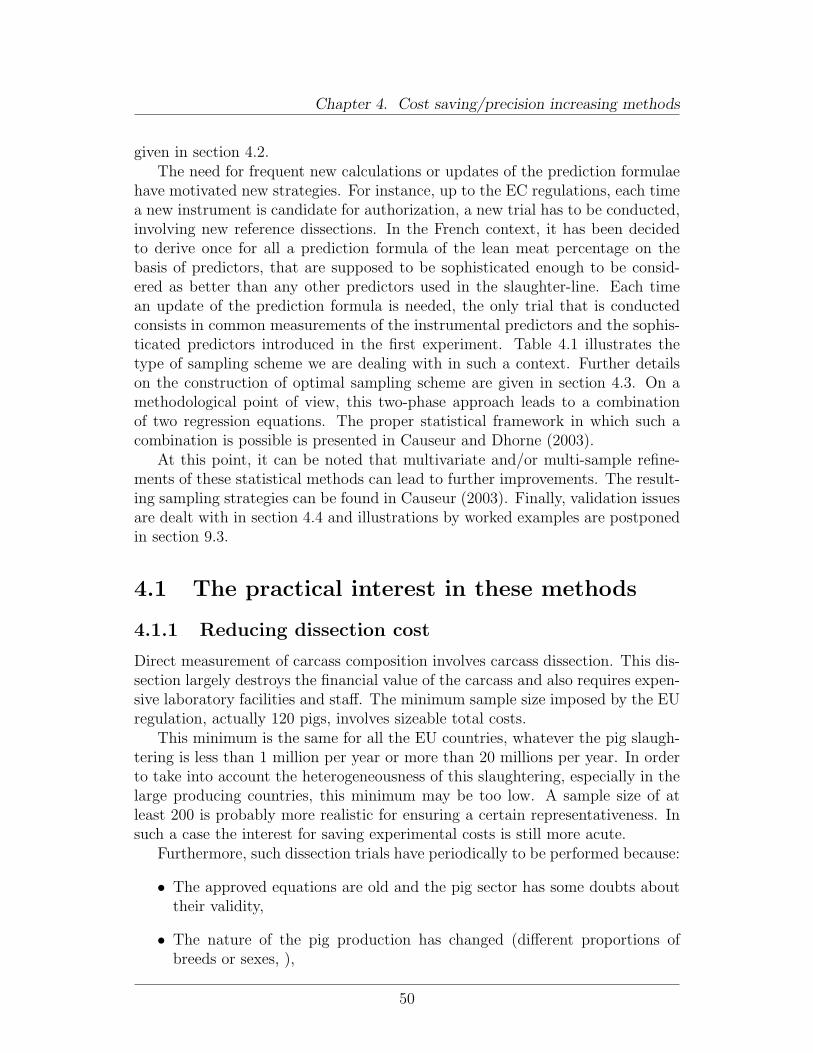
Chapter 4. Cost saving/precision increasing methods
given in section 4.2.The need for frequent new calculations or updates of the prediction formulae
have motivated new strategies. For instance, up to the EC regulations, each timea new instrument is candidate for authorization, a new trial has to be conducted,involving new reference dissections. In the French context, it has been decidedto derive once for all a prediction formula of the lean meat percentage on thebasis of predictors, that are supposed to be sophisticated enough to be consid-ered as better than any other predictors used in the slaughter-line. Each timean update of the prediction formula is needed, the only trial that is conductedconsists in common measurements of the instrumental predictors and the sophis-ticated predictors introduced in the first experiment. Table 4.1 illustrates thetype of sampling scheme we are dealing with in such a context. Further detailson the construction of optimal sampling scheme are given in section 4.3. On amethodological point of view, this two-phase approach leads to a combinationof two regression equations. The proper statistical framework in which such acombination is possible is presented in Causeur and Dhorne (2003).
At this point, it can be noted that multivariate and/or multi-sample refine-ments of these statistical methods can lead to further improvements. The result-ing sampling strategies can be found in Causeur (2003). Finally, validation issuesare dealt with in section 4.4 and illustrations by worked examples are postponedin section 9.3.
4.1 The practical interest in these methods
4.1.1 Reducing dissection cost
Direct measurement of carcass composition involves carcass dissection. This dis-section largely destroys the financial value of the carcass and also requires expen-sive laboratory facilities and staff. The minimum sample size imposed by the EUregulation, actually 120 pigs, involves sizeable total costs.
This minimum is the same for all the EU countries, whatever the pig slaugh-tering is less than 1 million per year or more than 20 millions per year. In orderto take into account the heterogeneousness of this slaughtering, especially in thelarge producing countries, this minimum may be too low. A sample size of atleast 200 is probably more realistic for ensuring a certain representativeness. Insuch a case the interest for saving experimental costs is still more acute.
Furthermore, such dissection trials have periodically to be performed because:
• The approved equations are old and the pig sector has some doubts abouttheir validity,
• The nature of the pig production has changed (different proportions ofbreeds or sexes, ),
50
Chapter 4. Cost saving/precision increasing methods
Design for double-regression
Sampling Lean meat % Approximate Instrumentalitem Lean meat % predictors
1 × × ×2 × × ×...
......
...n × × ×
n+1 ? × ×?
......
... ?...
...
?...
...
?...
...N ? × ×
Design for updates without new reference dissections
Sampling Lean meat % Sophisticated Instrumentalitem predictors predictors
1 × × ?2 × × ?...
......
...n × × ?
n+1 ? × ×?
......
... ?...
...
?...
...
?...
...N ? × ×
Table 4.1: Two-phase sampling scheme for updates without new reference dissec-tions. Missing values are figured by ?, observed values by ×.
51
Chapter 4. Cost saving/precision increasing methods
• A new classification instrument has to be tested,
• The EU definition of the LMP has changed.
There is evidence that the relationship between fat and muscle depths changeover time as well as between Member States. These changes suggest that morefrequent monitoring of the equations is necessary to ensure their continuing ac-curacy (Cook & Yates, 1992). Nevertheless, the expensive dissection procedurediscourages both the updating of the equations and the development of cheaperor more accurate measuring techniques.
So, the authors of the report on research concerning the harmonisation ofmethods for classification of pig carcases in the Community recommended toreduce the cost by the use of sample joint dissection and double regression. As aconsequence of this research double regression was introduced as the new standardof the statistical technique in the EU regulations in 1993-1994.
Since then, several Member States have used this method for assessing theirclassification methods. Works have been made for searching for the best concomi-tant variable(s) and for optimizing the sample sizes. One of the best solution useduntil now consists in removing the subcutaneous fat of ham, loin and shoulderand to build several concomitant variables from these weights. The major con-straint is the minimum sub-sample size of 50 imposed by the EU regulation inorder to ensure a certain representativeness. Using efficient concomitant vari-ables the total sample size may be around 180. Such a design permits to cut theexperimental costs by 30% compared with 120 carcasses dissected according theEU reference. Furthermore, the increase of 50 % of the sample size (180 vs. 120)improves the representativeness.
This method may also be used as a mean for increasing the accuracy for afixed cost. Nevertheless, this case is less frequent in practice.
The statistical aspects of this method, called ”double regression”, are devel-oped in §5.2.
4.1.2 Testing several instruments
Several companies sell different classification instruments. They differ in theirtechnology, price, size, accuracy, All the slaughterhouses have not the same needs.So, most of the Member States are interested in testing several instruments.
Nevertheless, the present EU regulation specifies that the assessment of aclassification method is based on a sample of at least 120 carcases (or 50 in thesub-sample if double regression). Using the same sample for all the instrumentsis attractive. Unfortunately, it is difficult to manage a lot of equipments at thesame time. Moreover, most of the present instruments are invasive, which detersthe tissues. It means that a second instrument cannot measure the same variableas a first one. Sure, another location could be used for the second instrument.
52
Chapter 4. Cost saving/precision increasing methods
By the way on one hand, the companies often recommend the same locationand on the other hand, different locations for the instruments may decrease thecomparability of classification data of the pig producers.
So, some Member States have chosen to test only one instrument. This situ-ation has the main disadvantage to introduce a monopoly. Other Member Stateshave preferred to test a few equipments using ”surrogate locations”. Generally,these are either the same location but on the right side or another location at 1cm around the first hole. The former does not correspond to the real conditionsof use. As the equipments are manufactured for right-handlers one can expecta significant effect between measurements on right and left sides. The latterintroduces also an error because the depths are not homogeneous, especially be-tween 2 ribs. Furthermore, nobody until now has estimated these kinds of errorand taken into account when assessing the prediction equations. Such practicescannot therefore be recommended.
A Member State has preferred to perform a separate trial for 2 instruments.Experimental cost was therefore double.
France & Germany have introduced in the 80’ a strategy eliminating all thesedisadvantages. This strategy was based in a two-stage procedure based on theuse of a reference instrument, more accurate than the to be tested instruments.This has made possible to approve several instruments on a time period of someyears having only performed one dissection trial. Nevertheless, this procedure has2 disadvantages: obliging all the instruments to measure at the same location(s)and eventually modifying the instruments software after the calibration againstthe reference instrument.
For these reasons France has deepened its strategy introducing now a ref-erence method instead of a reference instrument. The difference is that eachinstrument may have its own measuring locations. For applying such a strategynew statistical developments were needed. The statistical aspects of this method,called ”surrogate predictor regression”, are developed in §5.3.
Thanks to this great improvement France has got the official approval of 3methods using different predictors, has calibrated several old methods and hasdeveloped different classification control methods. Some of the methods were notavailable at the dissection period which was the initial motivation to develop sucha procedure.
In a 5 years time around 10 equations have been assessed. This representsa colossal saving cost and time compared to a dissection trial for each method.With only 2 equipments to be tested the cost is nearly divided by 2 becausethe cost of the 2nd stage (instruments calibration) is negligible compared to thisof the 1st stage (dissection trial). The gain is therefore much more importantthan using double regression. Furthermore, surrogate predictor regression can becombined with double regression in order to reduce even more the costs.
53
Chapter 4. Cost saving/precision increasing methods
4.2 Double regression
4.2.1 Introduction
Double regression (from now on referred to as DR) is a potentially useful methodwhen a surrogate for the EC reference percentage (Walstra and Merkus, 1995) isavailable. With DR we can either considerably reduce the cost of dissection orincrease the precision of predictions without further experimental cost comparedto linear regression (from now on referred to as LR). The surrogate percentagemay take the form of a quick rough and ready national dissection method. Thereduction in cost (or increase in precision) is realized by reducing the numberof relatively expensive EC reference dissections and adding a larger number ofnational dissections in a double sampling scheme. The national method mustbe considerably cheaper than the EC reference method. Also, in addition tothe instrumental carcass measurements, the percentage obtained by the nationaldissection method should have considerable predictive power for the EC referencepercentage. Otherwise there will be little to gain with DR compared with LR.
In technical statistical terms the national lean meat percentage is a concomi-tant variable. DR has been generalized to the case of several concomitant vari-ables by Causeur and Dhorne (1998). In principle, any set of variables that isclosely connected to the EC reference percentage and is not intended to be in-cluded as prediction variables in the prediction formula, are a set of candidateconcomitant variables in DR. Here, attention will be restricted to the case of oneconcomitant variable only. For illustrative purposes we will assume that the con-comitant variable is the lean meat percentage obtained by a simplified, faster andcheaper national dissection method. When several candidate concomitant vari-ables are available, the most promising variable or a summary variable may beused in DR. DR with several concomitant variables may offer a markedly largerreduction in experimental cost compared with DR with one of the concomitantvariables only (Causeur and Dhorne, 1998). In Causeur and Dhorne (1998) thelean meat percentage of the ham offers a reduction in cost of 25%. The lean meatpercentages of the loin should and filet each offer a reduction of less than 5 %.However, all four concomitant variables together offer a reduction of 38 %. Somenotation before we proceed:
Y = EC reference lean meat percentage;
Y ∗ = faster and cheaper dissection method, e.g. a national method;
x1, x2, . . . = instrumental carcass measurements, e.g. a fat and muscledepth measurement.
The predictive power for the EC reference percentage of the national percentageY ∗, in addition to the instrumental measurements x1, x2, . . . is measured by thepartial correlation between Y and Y ∗ given x1, x2, . . . . This partial correlation
54
Chapter 4. Cost saving/precision increasing methods
must be sufficiently large, otherwise DR will offer no marked advantage over LR.Details will be discussed below.
The double sample consists of N carcasses that are dissected by the cheapnational method. From the N carcasses a typically much smaller subset of ncarcasses are also dissected according to the EC reference method. Practicalimplementation may consist of, say, n carcass halves being dissected first by thenational method and then further dissected by the EC reference method, whilean additional (N − n) carcasses are dissected by the national method only. Iffurther dissection from national to EC reference percentage is a problem, andcarcass halves are dissected, n out of the N other halves of the carcasses maybe dissected by the EC reference method. For example, N right carcass halvesmay be dissected by the cheap national method, while n out of the N availableleft carcass halves are dissected by the EC reference method. Some details aboutselection of carcasses and required sample sizes n and N will be provided below.
We will introduce DR with data from a dissection experiment carried outin 1986 in The Netherlands to derive a prediction formula for the EC lean meatpercentage with the Henessy Grading Probe (HGP). This was the first applicationof DR and predates the amendment of the EC regulations with respect to use ofDR. The instrumental measurements with the HGP were a back fat measurement(x1) and a muscle thickness (x2), both measured at the third to fourth fromlast rib position 6 cm from the dorsal mid line (Walstra, 1986). The surrogatepercentages Y ∗ were obtained by the IVO standard method (Walstra, 1980). Thisis a quick incomplete dissection method that takes about 45 minutes per carcasshalf.
4.2.2 Sampling
N = 200 right carcass halves were dissected according to the IVO standardmethod (Walstra, 1980). A sub sample of n = 20 of these carcasses halveswere further dissected according to the EC reference method. Please note thataccording to the regulations, at present a minimum sub sample size of n = 50carcasses is required for the EC reference dissections in DR.
Carcasses were selected on the basis of HGP back fat thickness (x1). At thetime it was decided to mimic a random sample. Five back fat classes were chosen.The numbers of dissected carcasses in these classes were chosen proportional tothe numbers in the population. An alternative sampling procedure would havebeen the 40-20-40 % sampling scheme that is popular in pig carcass classificationexperiments and mentioned elsewhere in the handbook. Carcasses were selectedfrom 5 slaughterhouses and 40 carcasses were selected from each slaughterhouse.In order to reduce batch effects, every 10th carcass in the slaughterline was mea-sured. The same team dissected all carcass halves. Twenty carcasses were dis-sected at a time and two of them were further dissected by the EC referencemethod. Further details may be found in Walstra (1986) and Engel & Walstra
55
Chapter 4. Cost saving/precision increasing methods
(1991a).
4.2.3 Calculations
This section is based on Engel and Walstra (1991a, b). The calculations are inthree steps. First of all we establish a regression formula for the total sample ofsize N = 200 with the IVO standard percentage Y ∗ as the dependent variableand the HGP fat and muscle depth measurements x1 and x2 as the explanatoryvariables.
Y ∗ = 65.64− 0.6762x1 + 0.0903x2, RSD1 = 1.79, N = 200. (4.1)
RSD1 is the estimated value of the residual standard deviation (the root fromthe mean sum of squares for residual). Second, we establish a regression formulafor the EC reference lean meat percentage Y with fat and muscle depth x1 andx2 and the IVO standard lean meat percentage Y ∗ as explanatory variables. Thisregression is based on the sub sample of n = 20 carcasses only.
Y = −12.3− 0.0564x1 + 0.0711x2 + 1.079Y ∗, RSD2 = 0.833, n = 20.(4.2)
In the third and last step we construct the final prediction formula for the ECreference lean meat percentage. We replace Y ∗ in (4.2) by the right hand side of(4.1):
Y = −12.3− 0.0564x1 + 0.0711x2 + 1.079 (65.64− 0.6762x1 + 0.0903x2) .
This yields
Y = 58.52− 0.786x1 + 0.168x2, n = 20 and N = 200. (4.3)
In Engel and Walstra (1991b) it is shown how simple approximations to thestandard errors for the estimated constant and coefficients can be obtained fromthe output of the two regression equations. These approximate standard errorsare based on large sample results. Simulations show that these approximationsare adequate. Exact results are also available (Causeur and Dhorne, 1998).
As a suitable substitute for the RMSE we calculate an estimate for the residualstandard deviation (RSD) of the final prediction formula (4.3):
RSD2 = RSD22 + γ2RSD2
1. (4.4)
The coefficient γ in expression (4.4) is the coefficient for the surrogate percentagein (4.2). So, in this example γ = 1.079. Furthermore, RSD1 and RSD2 are theresidual standard deviations in regressions (4.1) (total sample) and (4.2) (subsample). In this example RSD1 = 1.79 and RSD2 = 0.833. For the finalformula this yields:
RSD =√
(0.833)2 + (1.079)2(1.79)2 = 2.10.
56
Chapter 4. Cost saving/precision increasing methods
An estimator with smaller order of bias than the maximum likelihood estimator(4.4) is presented in Causeur and Dhorne (1998).
It is important to realize that DR offers an estimation procedure in combina-tion with a double sampling scheme for the same constant and coefficients andresidual standard deviation that are estimated by LR. Hence, DR is no remedyfor measurement instruments where the value of σ is too high! The value of σdepends on the pig population, the instrument and the measurements used, andis for LR and DR the same.
There is the temptation in DR to leave the fat and muscle depth measurementsout of regression (4.2). In that case, when the relationship between the ECreference and the national lean meat percentage has already been establishedin the past, no further EC reference dissections would be needed to authorize anew instrument. It would be enough to collect instrumental measurements andperform national dissections only. However, when the instrumental measurementsadd significantly to regression (2), such an approach may produce poor estimatesfor the constant and coefficients in the final regression formula and the true RSDmay be considerably underestimated. For details we refer to Engel and Walstra(1991b) and Engel (1987).
4.2.4 Required sample sizes n and N
In order to calculate the required sample sizes, we need to evaluate the partialcorrelation between the EC reference and the national lean meat percentage,given the instrumental carcass measurements. This partial correlation measurescorrelation between the EC and national lean meat percentages that is not al-ready explained through the instrumental carcass measurements. It is a measureof the contribution of Y ∗ to regression (4.2) in addition to the instrumental mea-surements, e.g. the HGP fat and muscle depth in the example.
The partial correlation, say ρ, can be estimated as follows:
ρ = γRSD1
RSD.
In the example: ρ = 1.079 ∗ 1.79/2.10 = 0.92. Suppose that we want DR to beas accurate as LR with a sample size of m EC reference dissections. In that casethe total cost of LR would be
CostLR = C ∗m.
Here, C is the cost of dissection of a carcass (half) by the EC reference method.It is assumed that the additional cost of the instrumental carcass measurementsis negligible. The following sample sizes are required:
n = m{1− (1− f)ρ2
}and N =
n
f,
57
Chapter 4. Cost saving/precision increasing methods
where
f = minimumof
√c
C − c
1− ρ2
ρ2and 1.
Here, c is the cost of dissection of a carcass (half) by the national method. Thesesample sizes are based on large sample approximations. Details may be foundin Engel & Walstra (1991a,b). In the derivation it is assumed that carcasses areeither selected at random or on the basis of the instrumental measurements. Thecarcasses for the sub sample are assumed to be selected according to the samesampling scheme as the total sample. For instance, suppose that the total sampleis based on selection with three back fat classes, where boundary values are equalto mean back fat plus or minus one standard deviation. Let the numbers in theclasses be 0.4*N , 0.2*N and 0.4*N for lean, average and fat pigs respectively.Then a fraction n / N of the carcasses in each class are randomly chosen to obtainthe sub sample. In practise, carcasses for the sub sample could be selected on thebasis of Y ∗ as well, in that case DR can be expected to be even more accurate.Hence, the calculations yield somewhat liberal sample sizes. Since the value of ρwill not be very well known, it will often be a ”guesstimate” close to the lowestvalue still considered likely. Consequently, some liberality in the sample sizes isnot a point of grave concern.
For example, suppose that m = 120 (the minimum required sample size forLR according to the EC regulations). Let C/c = 5 and ρ = 0.9. Then:
f =
√1
5− 1
1− (0.9)2
(0.9)2= 0.2422,
n = 120{1− (1− 0.2422)(0.9)2
}= 46.3,
N = 46.3/0.2422 = 191.3.
Suppose that we take n = 50 and N = 200. The cost for DR with furtherdissection from national to EC reference lean meat percentage is:
CostDR = 50 ∗ C + (200− 50) ∗ c = C ∗ (50 + 150 ∗ 0.2) = C ∗ 80
.So, in this example cost by DR are reduced by (CostLR −CostDR)/CostLR ∗
100 = {(120− 80)/120} ∗ 100 = 33% relative to LR.
4.3 Two-phase updates based on reference pre-
dictors
For convenience, we present the statistical framework in the case of only one in-strumental predictor x, say a fat depth and only one reference predictor z, say an
58
Chapter 4. Cost saving/precision increasing methods
approximated lean meat percentage obtained by a partial dissection. Moreover,y will denote the response, say the lean meat percentage obtained by a referencedissection.
In what follows, preliminaries concerning the regression models are first dis-cussed. Then we show how minimum cost strategies are achieved under therestrictions laid down by the EC-regulations.
4.3.1 Creating the prediction formula
Our aim is to derive the prediction formula of y by the instrumental predictor xon the basis of the following linear regression model:
y = β0 + β1x + ε,
where ε ∼ N(0, σ) stands for the residual error, β0 denotes the offset and β1 isthe slope coefficient. However, y and x are never measured on a common sample.Therefore, the prediction formula is achieved through two auxiliary regressionmodels. First, call reference model the following one:
y = γr,0 + γr,1z + εr,
where εr ∼ N(0, σr) stands for the residual error, γ0,r denotes the offset and γ1,r
is the slope coefficient.Similarly, call scaling model the following one:
z = γs,0 + γs,1x + εs,
where εs ∼ N(0, σs) stands for the residual error, γ0,s denotes the offset and γ1,s
is the slope coefficient.The regression experiments which are conducted to estimate the coefficients
of the auxiliary models are usually not simultaneous: first, γ0,r and γ1,r areestimated on a sample of size nr, and then, for instance when an instrument iscandidate for authorization, γ0,s and γ1,s are estimated on another sample of sizens.
Although it appears as very intuitive to combine transitively the auxiliaryregression equations to obtain a prediction formula for y by x, it is recalled byEngel and Walstra (1991) that this is generally misleading. To combine properlythe regression equations, the reference model must indeed include x among itspredictors. However, provided z is a better predictor of y than x, in the sense that(z, x) is as good a predictor as z, Causeur and Dhorne (2003) have shown thata transitive combination of the regression equations was appropriate. Therefore,the prediction formula can be derived as follows:
y = γ0,r + γ1,rz,
= γ0,r + γ1,r (γ0,s + γ1,sx) ,
= γ0,r + γ1,rγ0,s︸ ︷︷ ︸β0
+ γ1,rγ1,s︸ ︷︷ ︸β1
x.
59
Chapter 4. Cost saving/precision increasing methods
The previous formula only gives the proper way of combining regression coeffi-cients estimated on two separate samples. Causeur and Dhorne (2003) give theequivalent formulæ in the more frequent case of many x variables and many zvariables and the standard deviations in the special case the auxiliary regressionequations are fitted by OLS. These standard deviations are the main support toprovide minimum costs strategies.
As it is discussed in chapter 2, the estimation of the auxiliary regressioncoefficients can be performed using OLS, PLS, PCR or any other relevant method.
4.3.2 Minimum costs sampling scheme
A regression experiment is first conducted in order to have common measurementsof the response and the reference predictors. Let cyz denote the experimental costper sampled carcass in this regression experiment, usually the time needed toobtain the measurements. When a prediction formula has to be assessed on thebasis of instrumental predictors, a scaling experiment is performed, which consistsin common measurements of the reference and the instrumental predictors. Callczx the experimental cost per sampled carcass in this scaling experiment. Theoverall experimental cost which is engaged for assessing the prediction formula istherefore:
c = nrcyz + nsczx.
According to the EC-requirements, the statistical method which is used to fit theregression model has to be at least as accurate as the usual least-squares methodon a sample of n = 120 carcasses. This kind of requirements obviously appealfor the definition of a criterion which aim is to compare the efficiencies of a two-phase procedure and the usual least-squares method. Provided OLS is used tofit the auxiliary regression models, Causeur and Dhorne (2003) have proposed arelative efficiency criterion that can be considered as the ratio of the variancesof the estimators of the regression coefficients. For instance, if we focus on theslope coefficient b, this relative efficiency criterion turns out to be:
RE(b; n, nr, ns) =n
nr
(nr
ns
ρ2yz.x + (1− ρ2
yz.x)(1 + ρ2zx)
),
where ρ2yz.x = 1 − σ2
r/σ2 is the squared partial correlation coefficient between y
and z conditionally on x and ρ2zx is the squared correlation coefficient between z
and x.Provided prior values of ρ2
yz.x and ρ2zx are available, the 120 carcasses-equiva-
lent EC-requirement is therefore transposed in the following equation:
RE(b; 120, nr, ns) = 1.
In the French context of pigs classification, the only remaining unknown of thisequation is the sample size ns since nr has been chosen previously.
60

Chapter 4. Cost saving/precision increasing methods
4.4 Validation issues
Many aspects of the validation of prediction formulæ have already been dis-cussed in chapter 2. Among the recommendations that have emerged from thediscussions, the use of the RMSEP have been proposed as a validation criterion.Therefore, in the present situation of double-sampling, validation will also beconsidered according to this choice.
First, note that, on the basis of the techniques that are mentioned in section2, it is clear that auxiliary RMSEP can be calculated. Call RMSEPy the RMSEPrelated to the auxiliary model including y and RMSEPz the RMSEP related tothe auxiliary model including only z. It can be shown, at least approximately ifthe sample sizes are large enough, that the global RMSEP used to validate theprediction formula estimated by a double-sampling method can be deduced fromthe following combination:
RMSEP 2 = RMSEP 2y + γ2RMSEP 2
z ,
where γ stands for the slope coefficient of z in the auxiliary model includingy. In the preceding equation, not only the auxiliary RMSEP can be calculatedwhatever the estimation procedure is used to fit the auxiliary models but alsothe estimated slope coefficient γ.
61


Chapter 5
Reporting to the Commission.Protocol for the trial
By Gerard Daumas
The present EU regulation lays out:“Part one of the protocol should give a detailed description of the dissection
trial and include in particular:
1. the trial period and time schedule for the whole authorization procedure,
2. the number and location of the abattoirs,
3. the description of the pig population concerned by the assessment method,
4. a presentation of the statistical methods used in relation to the samplingmethod chosen,
5. the description of the national quick method,
6. the exact presentation of the carcasses to be used.”
These items have not been specifically discussed. Nevertheless, one can lookfor the following items at the corresponding sections:
• Item 2: see section 1.2.2.
• Item 3: see section 1.1.
• Item 4: see chapters 2 and 4.
63


Part II
During and after the trial
65


Chapter 6
Some general comments on themanagement of the trial
By Gerard Daumas
During the trial a certain number of problems can occur which could affectthe quality of the results. In general, decisions have to be taken very quicklybecause of practical constraints. It is therefore very important that the benchscientist would be aware of all the issues, inclusive the statistical issues, in orderto get an acceptable compromise.
Some of the main problems occurring in classification experiments are asfollows:
• staff unavailability,
• abattoir unavailability,
• missing pigs in some categories for selection,
• instrument failure,
• changes in some environmental parameters,
• changes in work quality,
• wrong measurements,
• mixture of joints between carcasses,
• mixture of tissues between joints,
• mixture of tissues between carcasses.
These problems can be split into 2 categories according their consequences:
67

Chapter 6. Some general comments on the management of the trial
• selection of the pigs,
• data reliability.
Selection of the pigs
If there is a selection on factors (sex, breed, ) it can be difficult sometimesto find the needed category. This can lead to proportions different as initiallyplanned, affecting therefore the representativeness of the sample and introducingan overall bias.
Afterwards, this bias can be removed by a re-weighting of the observations atthe estimation stage. Nevertheless, it is important to avoid such changes in theproportions, especially for the small categories.
When there is an over-sampling at the extremes of predictor(s) some days itcan be very difficult to find the right pigs. The risk is all the more high sinceover-sampling intensity is high, the number of concerned predictors is high, thedaily number of selected carcasses is high and the slaughtering is low. This maylead to accept some pigs with some defects, especially an uncorrect splitline.In order to avoid a lower data reliability it is preferable to decrease the over-sampling intensity. Indeed, the latter has only an effect on the estimators variance; moreover, this effect is relatively small in the current designs for dissection trials.
Data reliability
Concerning the lean meat proportion (LMP)
The lean meat proportion may be affected by a lot of events for 2 reasons:
• it is not a direct measurement but a calculated variable from a lot of vari-ables,
• the measurement of all these variables is spread over several hours.
As the LMP is very expensive, temptation is high to conserve a carcass with awrong measurement. These wrong measurements may affect either joint weightsor tissue weights. It is therefore very important to check the data at each stage.After jointing a first check consists in calculating the jointing losses before startingdissection. In case of too high losses each joint can be weighted again. The sameholds for the dissection of the 4 joints. After dissection of a joint the dissectionlosses have to be calculated before throwing the different tissues in a tank wherethere are mixed with the tissues of other joints and other carcasses.
Some errors are more difficult to detect when they come from a (more orless) continuous change. For instance, the laborious dissection work can have apoorer quality in the afternoon or at the end of the week. This can be avoided
68

Chapter 6. Some general comments on the management of the trial
by the planning of a reasonable time schedule and by a supervising of the dis-section team. Some changes in the environmental conditions, like for instancethe temperature, may affect losses and the hardness of the work. It is there-fore recommended to write down some environmental parameters, some carcasscharacteristics and in general all kind of events which could help to explain somedoubtful data observed during the data processing.
Concerning the predictors
The statistical methods used until now in the pig classification context assumethere is no error on the independent variables. In fact, this is not the case withthe actual classification instruments.
Most of these instruments measure fat and muscle depths, muscle depth beingmore difficult to measure accurately. Moreover, these errors are not independent,because there is a common limit between fat and muscle tissues. Furthermore,some errors, especially on muscle depth, may be very high (5 or 10 mm).
But it is not always easy to immediately detect such errors. It means thatthis problem can be solved with the outliers management (see chapter 7).
The most dramatic incident is the failure of the tested instrument. Replacingequipment has to be foreseen.
69


Chapter 7
Departures from the model(lack-of-fit)
By Bas Engel
Although the average of the estimated error terms εi is always 0 for LR,lack of fit may be detected by plotting the individual estimates εi (referred to asresiduals) against the predictions yi (often referred to as fitted values). Accordingto standard theory fitted values and residuals are uncorrelated for LR and nearlyso for non-linear regression. This implies that in the aforementioned residualplot, there should be no obvious pattern, when the regression model fits thedissection data well. If there is a pattern, this may indicate some serious departurefrom the model assumptions. For instance, an increase of the absolute residualswith an increase of the fitted values, suggests that the residual variance is notconstant. A simple remedy may be to replace observations y by log-transformedobservations log(y). However, this is not always an appropriate remedy, eitherbecause heterogeneity of variances may remain, or because a LR model may nolonger apply after transformation. In that case the use of non-linear regressionor the use of a variance function may be considered. A curve in the residual plotmay indicate the need for a quadratic term x2 in the model. So far, there is noevidence supplied for marked variance heterogeneity or curvi-linearity.
Since y and y are strongly correlated, it is generally a better idea to supplya plot of residuals e against y, rather than a plot of y against y. Unfortunately,the last plot has been a regular feature in many proposals so far.
Departures from normality may be apparent from a so-called probability plotof the residuals. Residuals are ordered in increasing size and plotted againsttheir expected values under normality. Departures from a straight line, usuallyin the form of a sigmoid curve, indicate non-normality. These plots tend tobe more informative than formal tests of significance. Non-normality is generallyconsidered to be a less serious problem than heterogeneity of variances or apparentlack of additional predictors such as quadratic terms x2 in the formula.
71


Chapter 8
Managing outliers
By Thierry Dhorne
8.1 Aim
The elaboration of “good” models for pig classification is achieved by two statis-tical means:
• specifying and using models with good theoretical properties,
• adjusting the models in the best way in the best way.
Both are the major aims of the present handbook.The last (and not the less) point is to get good datas to adjust the model.
Many things are suggested by meat scientists to obtain good datas and we willconcentrate here on the specific aspect of assessing in some way the quality ofthe data obtained in a trial in order to get reliable prediction formulas.
It is important to make a difference between what is acceptable (for instancewith respect to the regulation) and what is reliable.
The aim now is then to deal with the management of both observations that:
• have a great influence on the assessment of the formula and/or
• are badly predicted by the TVM prediction formula.
8.2 The issue
As mentioned above, the problem is that quality is more or less subjective andthat two scientists could consider as different the same situation.
We will then concentrate here on the way to detect problems and leave thedecision of interpreting the problems to meat scientists.
73
Chapter 8. Managing outliers
Let us then mention clearly the issues: what can be thought of a formula equa-tion in some countries where one carcass, or five or twenty-five out of a hundredis (are) really badly predicted ? Suppose that the formula for the fair carcasseshas a standard-error of let say 2, and that the bad carcasses are predicted atrandom, let say with a standard-error of 3.5, to be compared with the 2.5 of theregulation. In the three cases (if it is assumed that the mean is known), we have:
1. 1 % bad predictions:√
99.22 + 1.3.52 = 2.02
2. 5 % bad predictions:√
95.22 + 5.3.52 = 2.10
3. 25 % bad predictions:√
75.22 + 25.3.52 = 2.46
and everything is all-right.Furthermore, what can be thought of a formula established on a set of a hun-
dred carcasses and where the deletion of one, three, nine carcasses in the samplecould change the equation in a sensible way for the millions of pigs classified everyyear.
The objective of this part is to evaluate the importance of these two issuesand to give some solutions to them.
8.3 Definitions
Though the statistical vocabulary is not completely established in this field somemain key-words are important.
First the topic concerned is usually defined by robustness. This topic dealswith the capacity of the predictors to resist to practical factors that could decreasethe reliability of the model essentially because they invalidate assumptions madeby the statistician to choose it.
Due to the fact that prediction equations are always obtained explicitly orimplicitly through the minimization of a criterion of discrepancy between thereal observed values and the predicted values, it is clear that these errors in thedata can generate two different negative effects:
• some observations far from the others “attracts” the model through theminimization,
• some observations show a great discrepancy between the predicted andobserved values.
The first type of observations is usually refered as influential observations (orleverage points), the second type as outliers.
As mentioned above these two aspects are independent in the sense that thefour situations can be encountered, namely: standard observation (neither influ-ential nor outlying), outlier not influential, influential observation not outlying,influential outlier.
74
Chapter 8. Managing outliers
8.4 Statistical solutions
8.4.1 Graphical studies
It is probably the easiest way to deal with the problem as suggested by veryimpressive but specific graphics proposed here and there. This approach suggestsnevertheless problems of two kinds:
• first the subjectivity of the observer and then of the procedure,
• the difficulty to generalize this approach when the model is more complex(multivariate) and when many data sets are involved.
There was then a need to develop more technical methods to solve this problem.
8.4.2 Residuals analysis
Residuals analysis has been widely used for years in the treatment of regressiondata. Unfortunately this analysis is not suited to evaluate influential observationswhich has been shown above to be different with the outlier problems. Moreoverthe analysis is made after classical least squares adjustment. This strategy issomewhat paradoxical because the aim is to avoid influence of some points whilethe initial estimation may be widely influenced by these points in an undetectableway.
This points out that one single observation can pollute the other ones andattract to itself the regression line and leads to the interest of studying the indi-vidual influence of each point on the assessment of the regression.
8.4.3 Influence analysis
As defined previously, the influence of a single observation can be roughly definedas the discrepancy between the prediction formulae obtained on the one hand withthe whole dataset and on the other hand without this observation. Statisticalprocedures in influence analysis are mainly based on two formal interpretationsof the former definition of influence:
• individual influence can first be defined as the impact of a single observationon the prediction procedure: this approach is consistent with the detectionof influential observations,
• influence analysis can also consist in measuring the consequence of thedeletion of a single observation on the estimated parameters of the model:both outliers and influential observations can be pointed out throughoutthis approach.
75
Chapter 8. Managing outliers
8.4.4 Robust estimation
The naturel extension of influence analysis would be to try to study the influenceof couples of points, then triplets and so on, to avoid the joint effect of multipleinfluential observations. The limit should be the number of errors of any kindthat can be made in getting the data.
This aspect has led to the notion of breakdown point corresponding to thepercentage of contaminated data sufficient to “break” the “real” regression line.It is easy to appreciate intuitively this notion in the easier case of the estimationof the location parameter of a data set.
Let us examine a univariate series of values and consider the departure ofsome points to plus or minus infinity. It is obvious that in the case of the mean,one single observation can pull it to plus of minus infinity, whereas the mediancan be seen to resist up to nearly 50 % of the observations contaminated. It isthen said that the mean has a O % breakpoint while the median has a 50 %breakpoint.
In the field of multiple regression it has been a challenge for years to investigatethe existence of robust regression procedures that could improve the catastrophicbreak point of the usual least squares estimator.
The main ideas at the basis of such investigations are the following:
1. Though the problem seems to be quite easy for a location parameter (me-dian versus mean), it is not so obvious that a generalization holds for regres-sion parameters. It is known that not even a generalization of the medianis easily available for a two dimensional location parameter.
2. Furthermore even if this goal can be achieved, the example of the medianshows that protection against influential points has a cost at least in termof variance of estimators.
3. The idea that an exhaustive procedure that could identify every subset ofinfluential points conveys the impression that any robust procedure shouldlead to complex numberings and therefore to computer intensive procedures.
8.5 Robust estimation
The idea of robust estimation focused on the field of regression is then reallyappealing. Indeed, where the classical procedures make an adjustment and thenexamine the influential points with the risk that they are hidden by themselves, arobust procedure would give an adjustment free of influential points which wouldthen be implicitly identified. Furthermore it could enable the examination ofoutliers in a safe way.
The point is now to define such procedures.
76

Chapter 8. Managing outliers
8.5.1 Criteria
Two generations of criteria have been proposed in the literature to achieve theformer goals. One deals with influential functions of the observations, the otherwith general robust criterions.
Influence fonctions The classical least squares estimator is known to minimizethe quantity:
n∑i=1
(Yi − Yi)2 =
n∑i=1
e2i .
Global criterion One of the most significant result in robustness was workedby Rousseuw and Leroy (1987). It is also a very sensitive approach for nonstatisticians and therefore it can easily be understood.
The idea is simply to consider the former criterion:
n∑i=1
(Yi − Yi)2 =
n∑i=1
e2i ,
as its equivalent:
1/nn∑
i=1
e2i ,
the mean of the squares of the residuals, and then replace the mean by a morerobust quantity. Two variants have been proposed by Rousseuw and Leroy (1987):
• the median of squares:
medie2i ,
• the trimmed mean of squares:
h∑i=1
e2(i),
where e2(i) means the ascendant ordering of the residuals and n/2 ≤ h ≤ n.
Both variants are subject to minimization with respect to the regression param-eters, leading to so-called:
1. least median of squares estimator: LMS,
2. least trimmed squares estimator (the fraction of trim being h/n): LTS.
77
Chapter 8. Managing outliers
8.5.2 Efficiency
The efficiency of such procedures has been studied theoretically. The LTS esti-mator has been shown to be more efficient than the LMS estimator and to be asefficient (up to a constant) as the classical LS estimator.
It can therefore be recommended to use the LTS estimator even with a highlevel of protection i.e. 50 %.
8.5.3 Algorithm
As suspected before, the global minimum of such a quantity as trimmed squaresof the residual is not so easy to reach. Indeed iterative methods must be usedbut nevertheless two points should be pointed out:
1. there exists generally many local minima to the objective function,
2. there exists no obvious initial value for an iterative method, and in partic-ular, least squares solution is generally a bad initial value leading to a localminimum.
Fortunately, many softwares implementation are now available and consequentimprovements have been made. Such procedures are indeed available in S/R orSAS systems.
8.5.4 Protocol
In practice, what is to be down ?
• First accept that a part of the data may be spoiled or what is equivalentaccept to leave out part of the data in order to have more confidence onthe prediction formula.
The percentage suggested is about 5 % (former studies of the homologationreports gives an interval of 3 to 7 %). A more precise study could be to letthe percentage vary from say 2 to 10 % in order to get a best appreciationof the real percentage.
• Then use least trimmed squares procedures to adjust regression (or equiv-alent other method: for PLS minimal volume estimation can be used) andidentify influent data by decreasing order of influence.
• Status then on these data (are they considered as acceptable or not ?),some arguments should be given here and specially reference to informationobtained during the trial.
• Perform the classical (without outliers and influential observations) on therestricted set of data.
78

Chapter 8. Managing outliers
• Calculate the required criterion (RMSEP) with the suspicious data consid-ered in the calculation.
79

Chapter 9
Estimation and validation inpractice. Examples
By David Causeur, Bas Engel, Maria Font i Furnols and Søren Højsgaard
9.1 Available software
It would be too ambitious to pretend proposing a comprehensive list of the solu-tions to actually run rank-reduced methods for many softwares have been editedsince the first one in the mid-1980s. This pioneering software, called LVPLS,was for a long time the only solution for practitioners. The current version runsin DOS and is freely distributed by Mc Ardle J. (1987). We are only intendinghere to list some packages that can be used to establish prediction formulæwithrank-reduced methods. Furthermore, we have chosen to focus on PLS packagessince OLS functions are usually included in all the statistical softwares and alsosince PCR functions are most of the times delivered in the PLS packages.
Some widely spread statistical softwares such as SAS or Splus propose theirown PLS packages. For instance, the SAS system version 6.11 includes an exper-imental PROC PLS and version 8 has the definitive one. Online documentation(in Adobe PDF format) is available by Tobias R.D. (1997a, 1997b). At the sametime, public domain PLS procedures were also developed, initially for the non-commercial version of Splus called R (that can be downloaded at http://cran.r-project.org/). The idea behind R is clearly to propose a free copy of the Splusprogramming environment. However, note that in the last ten years, Splus haveimproved its commercial attractiveness by adopting a Windows-like aspect whichmakes it possible to run some usual data analysis through toolbars and dialogboxes instead of the programming environment. The PLS package is currentlynot running through toolbars but only in the programming environment. Thispackage was based on Denham (1995) and can be downloaded freely (the free
81
Chapter 9. Estimation and validation in practice. Examples
download at http://cran.r-project.org/src/contrib/Devel/ includes minimal doc-umentation). A port of a Denham (1995)s S/S-Plus implementation is available inthe Carnegie-Mellon S archive (http://lib.stat.cmu.edu/S/), which also includesFortran and Matlab implementations of the algorithm.
Finally, it must be noted that GENSTAT 5 (details about this software canbe found at http://www.nag.co.uk/stats/TT soft.asp) implements PLS and alsothat some other commercial software especially dedicated to PLS analysis areuntil recently available. Most of the times, they enable a more detailed exami-nation of the prediction properties. Their working environment is quite easy todiscover since all the analysis are available by toolbars, whereas SAS or R/Splusappeals for a prior knowledge of the programming environment. As an example,The Unscrambler from Camo Inc (www.camo.no) implements PLS, includingjackknife-based significance testing.
9.2 A worked example
9.2.1 Description of data
The ideas and models discussed below have been evaluated on a small datasetconsisting of measurements on 344 carcasses delivered to three Danish abattoirs.At two abattoirs, 150 normal carcasses were measured. At the third abattoiradditionally 44 large carcasses were measured. The distribution of the carcassesamong the three slaughterhouses and in different weight groups is shown in Ta-ble 9.1 together with the average LMP.
Table 9.1: Distribution of carcasses among the three slaughterhouses and in dif-ferent weight groups and the average LMP.
Abattoir (60,70] (70,75] (75,80] (80,90] (90,105] LMP1 35 54 43 18 0 59.22 35 48 41 26 0 59.73 0 0 0 17 27 58.7
Fat and meat depth was measured on several locations together with slaughterweight, length and other physical characteristics. The locations of the measure-ments are shown in Figure 9.1.
9.2.2 Doing it in R/Splus
Preliminaries: general issues on R and Splus
Most of the commands that are used in the programming environment canroughly be described by the following generic command:
82
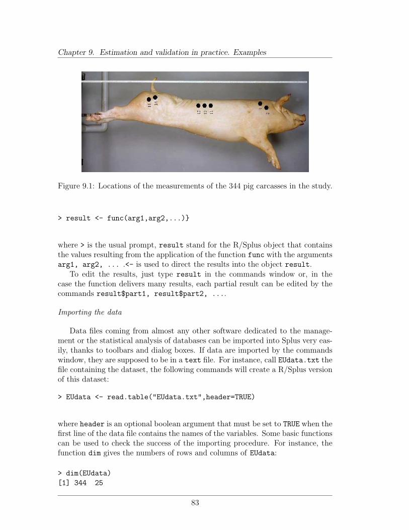
Chapter 9. Estimation and validation in practice. Examples
Figure 9.1: Locations of the measurements of the 344 pig carcasses in the study.
> result <- func(arg1,arg2,...)}
where > is the usual prompt, result stand for the R/Splus object that containsthe values resulting from the application of the function func with the argumentsarg1, arg2, ... .<- is used to direct the results into the object result.
To edit the results, just type result in the commands window or, in thecase the function delivers many results, each partial result can be edited by thecommands result$part1, result$part2, ....
Importing the data
Data files coming from almost any other software dedicated to the manage-ment or the statistical analysis of databases can be imported into Splus very eas-ily, thanks to toolbars and dialog boxes. If data are imported by the commandswindow, they are supposed to be in a text file. For instance, call EUdata.txt thefile containing the dataset, the following commands will create a R/Splus versionof this dataset:
> EUdata <- read.table("EUdata.txt",header=TRUE)
where header is an optional boolean argument that must be set to TRUE when thefirst line of the data file contains the names of the variables. Some basic functionscan be used to check the success of the importing procedure. For instance, thefunction dim gives the numbers of rows and columns of EUdata:
> dim(EUdata)
[1] 344 25
83
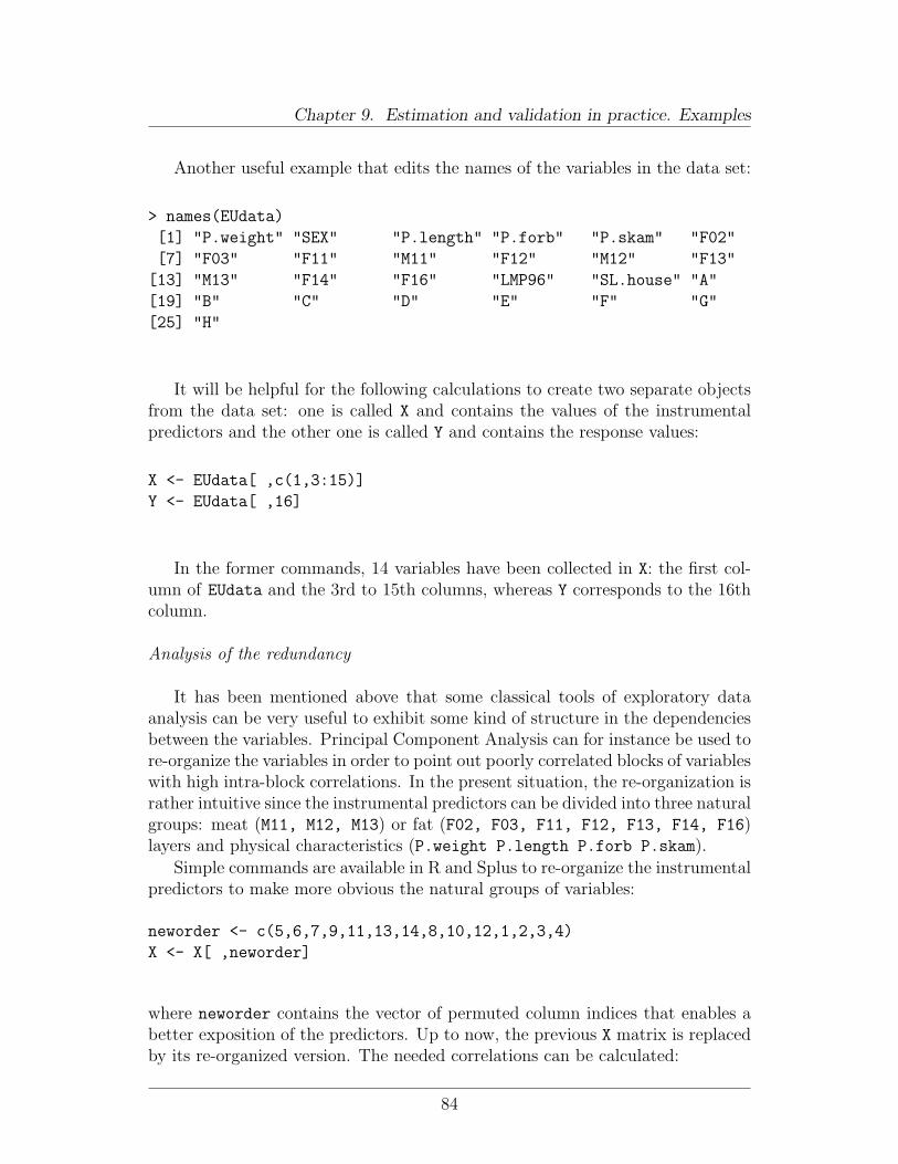
Chapter 9. Estimation and validation in practice. Examples
Another useful example that edits the names of the variables in the data set:
> names(EUdata)
[1] "P.weight" "SEX" "P.length" "P.forb" "P.skam" "F02"
[7] "F03" "F11" "M11" "F12" "M12" "F13"
[13] "M13" "F14" "F16" "LMP96" "SL.house" "A"
[19] "B" "C" "D" "E" "F" "G"
[25] "H"
It will be helpful for the following calculations to create two separate objectsfrom the data set: one is called X and contains the values of the instrumentalpredictors and the other one is called Y and contains the response values:
X <- EUdata[ ,c(1,3:15)]
Y <- EUdata[ ,16]
In the former commands, 14 variables have been collected in X: the first col-umn of EUdata and the 3rd to 15th columns, whereas Y corresponds to the 16thcolumn.
Analysis of the redundancy
It has been mentioned above that some classical tools of exploratory dataanalysis can be very useful to exhibit some kind of structure in the dependenciesbetween the variables. Principal Component Analysis can for instance be used tore-organize the variables in order to point out poorly correlated blocks of variableswith high intra-block correlations. In the present situation, the re-organization israther intuitive since the instrumental predictors can be divided into three naturalgroups: meat (M11, M12, M13) or fat (F02, F03, F11, F12, F13, F14, F16)layers and physical characteristics (P.weight P.length P.forb P.skam).
Simple commands are available in R and Splus to re-organize the instrumentalpredictors to make more obvious the natural groups of variables:
neworder <- c(5,6,7,9,11,13,14,8,10,12,1,2,3,4)
X <- X[ ,neworder]
where neworder contains the vector of permuted column indices that enables abetter exposition of the predictors. Up to now, the previous X matrix is replacedby its re-organized version. The needed correlations can be calculated:
84
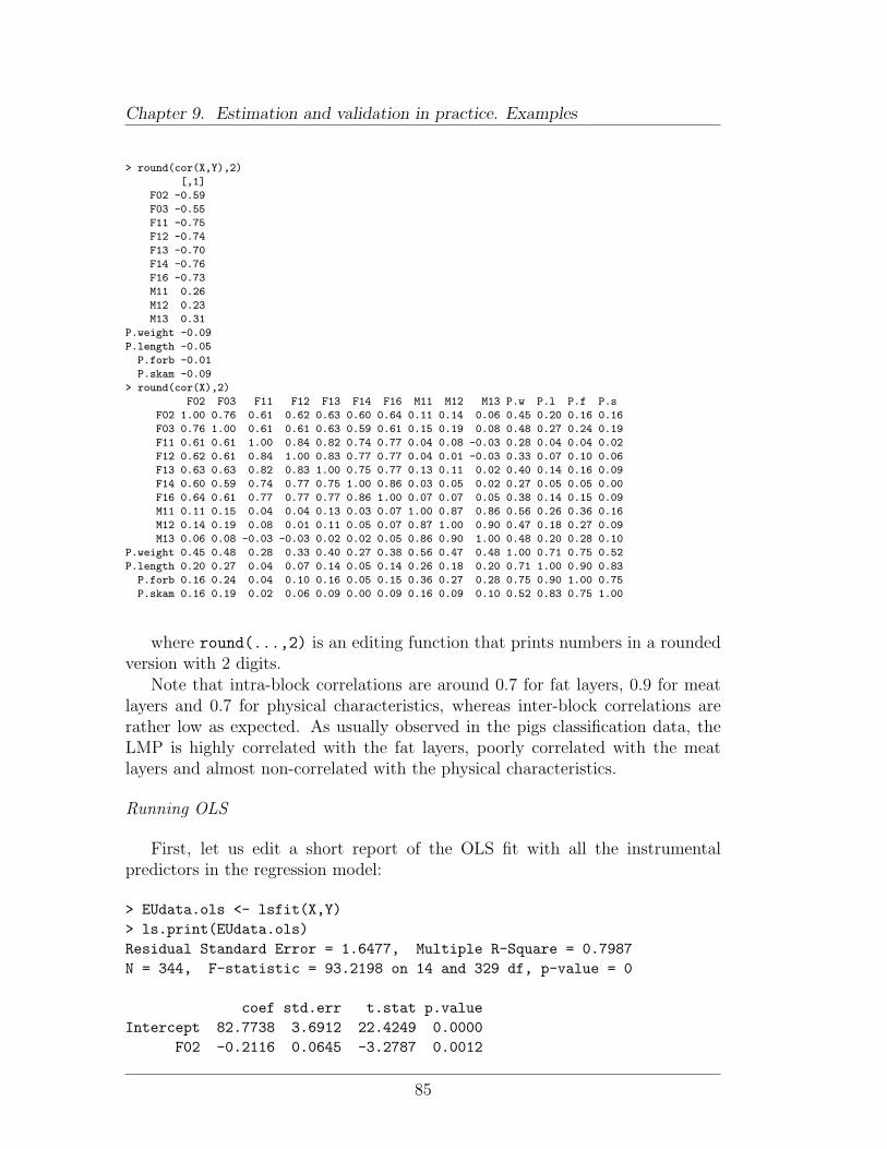
Chapter 9. Estimation and validation in practice. Examples
> round(cor(X,Y),2)
[,1]
F02 -0.59
F03 -0.55
F11 -0.75
F12 -0.74
F13 -0.70
F14 -0.76
F16 -0.73
M11 0.26
M12 0.23
M13 0.31
P.weight -0.09
P.length -0.05
P.forb -0.01
P.skam -0.09
> round(cor(X),2)
F02 F03 F11 F12 F13 F14 F16 M11 M12 M13 P.w P.l P.f P.s
F02 1.00 0.76 0.61 0.62 0.63 0.60 0.64 0.11 0.14 0.06 0.45 0.20 0.16 0.16
F03 0.76 1.00 0.61 0.61 0.63 0.59 0.61 0.15 0.19 0.08 0.48 0.27 0.24 0.19
F11 0.61 0.61 1.00 0.84 0.82 0.74 0.77 0.04 0.08 -0.03 0.28 0.04 0.04 0.02
F12 0.62 0.61 0.84 1.00 0.83 0.77 0.77 0.04 0.01 -0.03 0.33 0.07 0.10 0.06
F13 0.63 0.63 0.82 0.83 1.00 0.75 0.77 0.13 0.11 0.02 0.40 0.14 0.16 0.09
F14 0.60 0.59 0.74 0.77 0.75 1.00 0.86 0.03 0.05 0.02 0.27 0.05 0.05 0.00
F16 0.64 0.61 0.77 0.77 0.77 0.86 1.00 0.07 0.07 0.05 0.38 0.14 0.15 0.09
M11 0.11 0.15 0.04 0.04 0.13 0.03 0.07 1.00 0.87 0.86 0.56 0.26 0.36 0.16
M12 0.14 0.19 0.08 0.01 0.11 0.05 0.07 0.87 1.00 0.90 0.47 0.18 0.27 0.09
M13 0.06 0.08 -0.03 -0.03 0.02 0.02 0.05 0.86 0.90 1.00 0.48 0.20 0.28 0.10
P.weight 0.45 0.48 0.28 0.33 0.40 0.27 0.38 0.56 0.47 0.48 1.00 0.71 0.75 0.52
P.length 0.20 0.27 0.04 0.07 0.14 0.05 0.14 0.26 0.18 0.20 0.71 1.00 0.90 0.83
P.forb 0.16 0.24 0.04 0.10 0.16 0.05 0.15 0.36 0.27 0.28 0.75 0.90 1.00 0.75
P.skam 0.16 0.19 0.02 0.06 0.09 0.00 0.09 0.16 0.09 0.10 0.52 0.83 0.75 1.00
where round(...,2) is an editing function that prints numbers in a roundedversion with 2 digits.
Note that intra-block correlations are around 0.7 for fat layers, 0.9 for meatlayers and 0.7 for physical characteristics, whereas inter-block correlations arerather low as expected. As usually observed in the pigs classification data, theLMP is highly correlated with the fat layers, poorly correlated with the meatlayers and almost non-correlated with the physical characteristics.
Running OLS
First, let us edit a short report of the OLS fit with all the instrumentalpredictors in the regression model:
> EUdata.ols <- lsfit(X,Y)> ls.print(EUdata.ols)Residual Standard Error = 1.6477, Multiple R-Square = 0.7987N = 344, F-statistic = 93.2198 on 14 and 329 df, p-value = 0
coef std.err t.stat p.valueIntercept 82.7738 3.6912 22.4249 0.0000
F02 -0.2116 0.0645 -3.2787 0.0012
85
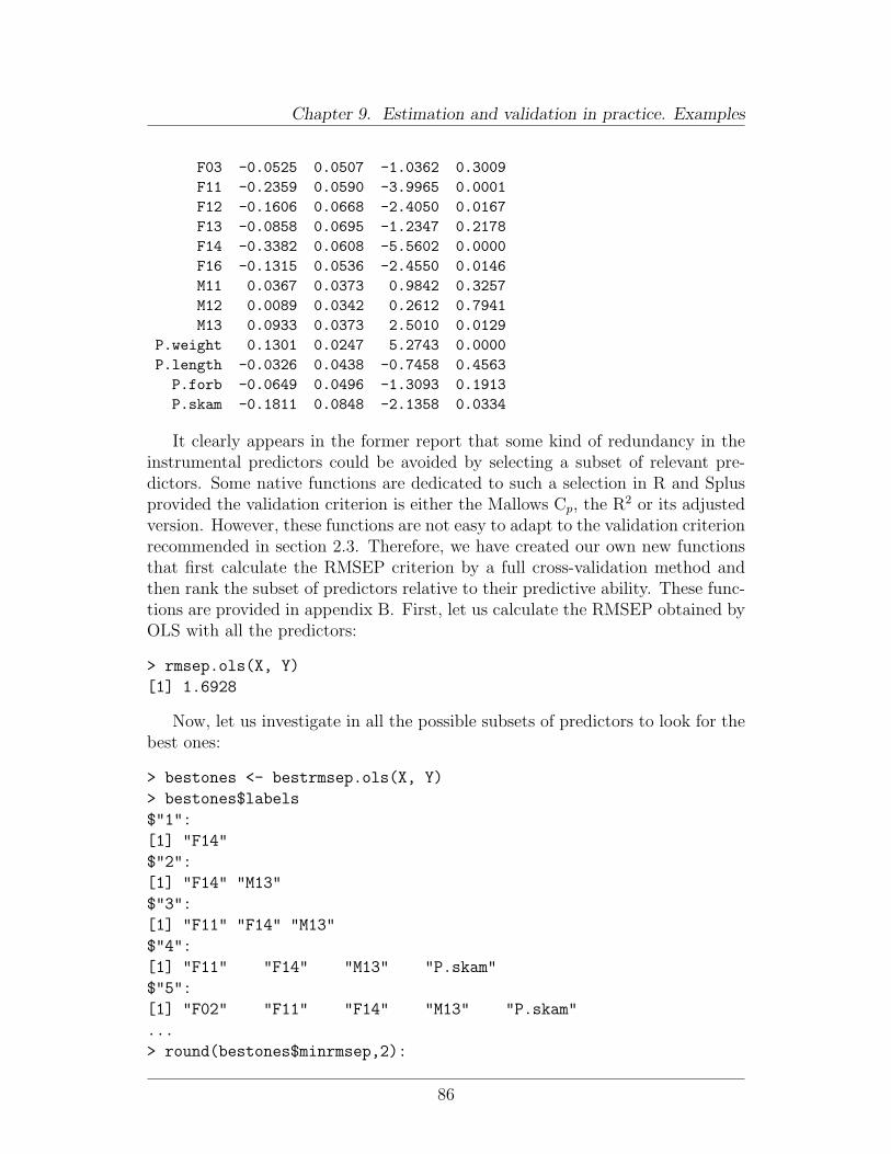
Chapter 9. Estimation and validation in practice. Examples
F03 -0.0525 0.0507 -1.0362 0.3009F11 -0.2359 0.0590 -3.9965 0.0001F12 -0.1606 0.0668 -2.4050 0.0167F13 -0.0858 0.0695 -1.2347 0.2178F14 -0.3382 0.0608 -5.5602 0.0000F16 -0.1315 0.0536 -2.4550 0.0146M11 0.0367 0.0373 0.9842 0.3257M12 0.0089 0.0342 0.2612 0.7941M13 0.0933 0.0373 2.5010 0.0129
P.weight 0.1301 0.0247 5.2743 0.0000P.length -0.0326 0.0438 -0.7458 0.4563
P.forb -0.0649 0.0496 -1.3093 0.1913P.skam -0.1811 0.0848 -2.1358 0.0334
It clearly appears in the former report that some kind of redundancy in theinstrumental predictors could be avoided by selecting a subset of relevant pre-dictors. Some native functions are dedicated to such a selection in R and Splusprovided the validation criterion is either the Mallows Cp, the R2 or its adjustedversion. However, these functions are not easy to adapt to the validation criterionrecommended in section 2.3. Therefore, we have created our own new functionsthat first calculate the RMSEP criterion by a full cross-validation method andthen rank the subset of predictors relative to their predictive ability. These func-tions are provided in appendix B. First, let us calculate the RMSEP obtained byOLS with all the predictors:
> rmsep.ols(X, Y)
[1] 1.6928
Now, let us investigate in all the possible subsets of predictors to look for thebest ones:
> bestones <- bestrmsep.ols(X, Y)
> bestones$labels
$"1":
[1] "F14"
$"2":
[1] "F14" "M13"
$"3":
[1] "F11" "F14" "M13"
$"4":
[1] "F11" "F14" "M13" "P.skam"
$"5":
[1] "F02" "F11" "F14" "M13" "P.skam"
...
> round(bestones$minrmsep,2):
86
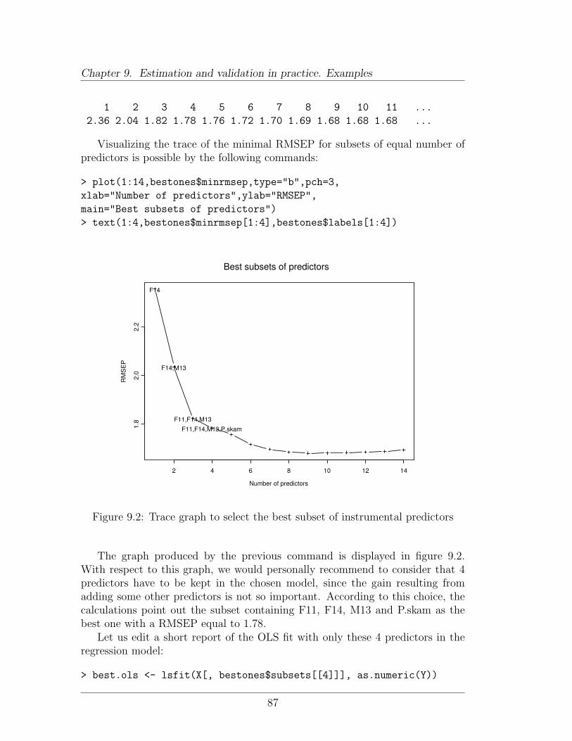
Chapter 9. Estimation and validation in practice. Examples
1 2 3 4 5 6 7 8 9 10 11 ...
2.36 2.04 1.82 1.78 1.76 1.72 1.70 1.69 1.68 1.68 1.68 ...
Visualizing the trace of the minimal RMSEP for subsets of equal number ofpredictors is possible by the following commands:
> plot(1:14,bestones$minrmsep,type="b",pch=3,
xlab="Number of predictors",ylab="RMSEP",
main="Best subsets of predictors")
> text(1:4,bestones$minrmsep[1:4],bestones$labels[1:4])
Best subsets of predictors
Number of predictors
RM
SE
P
2 4 6 8 10 12 14
1.8
2.0
2.2
F14
F14,M13
F11,F14,M13F11,F14,M13,P.skam
Figure 9.2: Trace graph to select the best subset of instrumental predictors
The graph produced by the previous command is displayed in figure 9.2.With respect to this graph, we would personally recommend to consider that 4predictors have to be kept in the chosen model, since the gain resulting fromadding some other predictors is not so important. According to this choice, thecalculations point out the subset containing F11, F14, M13 and P.skam as thebest one with a RMSEP equal to 1.78.
Let us edit a short report of the OLS fit with only these 4 predictors in theregression model:
> best.ols <- lsfit(X[, bestones$subsets[[4]]], as.numeric(Y))
87
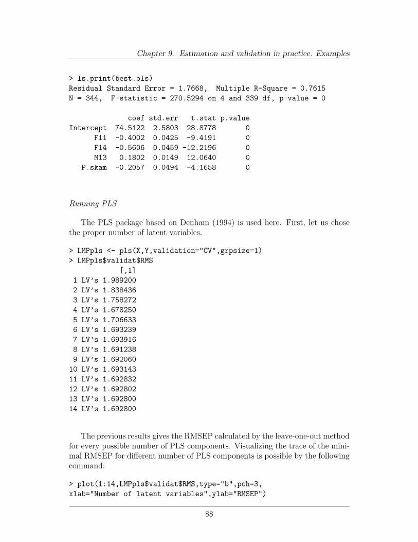
Chapter 9. Estimation and validation in practice. Examples
> ls.print(best.ols)
Residual Standard Error = 1.7668, Multiple R-Square = 0.7615
N = 344, F-statistic = 270.5294 on 4 and 339 df, p-value = 0
coef std.err t.stat p.value
Intercept 74.5122 2.5803 28.8778 0
F11 -0.4002 0.0425 -9.4191 0
F14 -0.5606 0.0459 -12.2196 0
M13 0.1802 0.0149 12.0640 0
P.skam -0.2057 0.0494 -4.1658 0
Running PLS
The PLS package based on Denham (1994) is used here. First, let us chosethe proper number of latent variables.
> LMPpls <- pls(X,Y,validation="CV",grpsize=1)
> LMPpls$validat$RMS
[,1]
1 LV’s 1.989200
2 LV’s 1.838436
3 LV’s 1.758272
4 LV’s 1.678250
5 LV’s 1.706633
6 LV’s 1.693239
7 LV’s 1.693916
8 LV’s 1.691238
9 LV’s 1.692060
10 LV’s 1.693143
11 LV’s 1.692832
12 LV’s 1.692802
13 LV’s 1.692800
14 LV’s 1.692800
The previous results gives the RMSEP calculated by the leave-one-out methodfor every possible number of PLS components. Visualizing the trace of the mini-mal RMSEP for different number of PLS components is possible by the followingcommand:
> plot(1:14,LMPpls$validat$RMS,type="b",pch=3,
xlab="Number of latent variables",ylab="RMSEP")
88
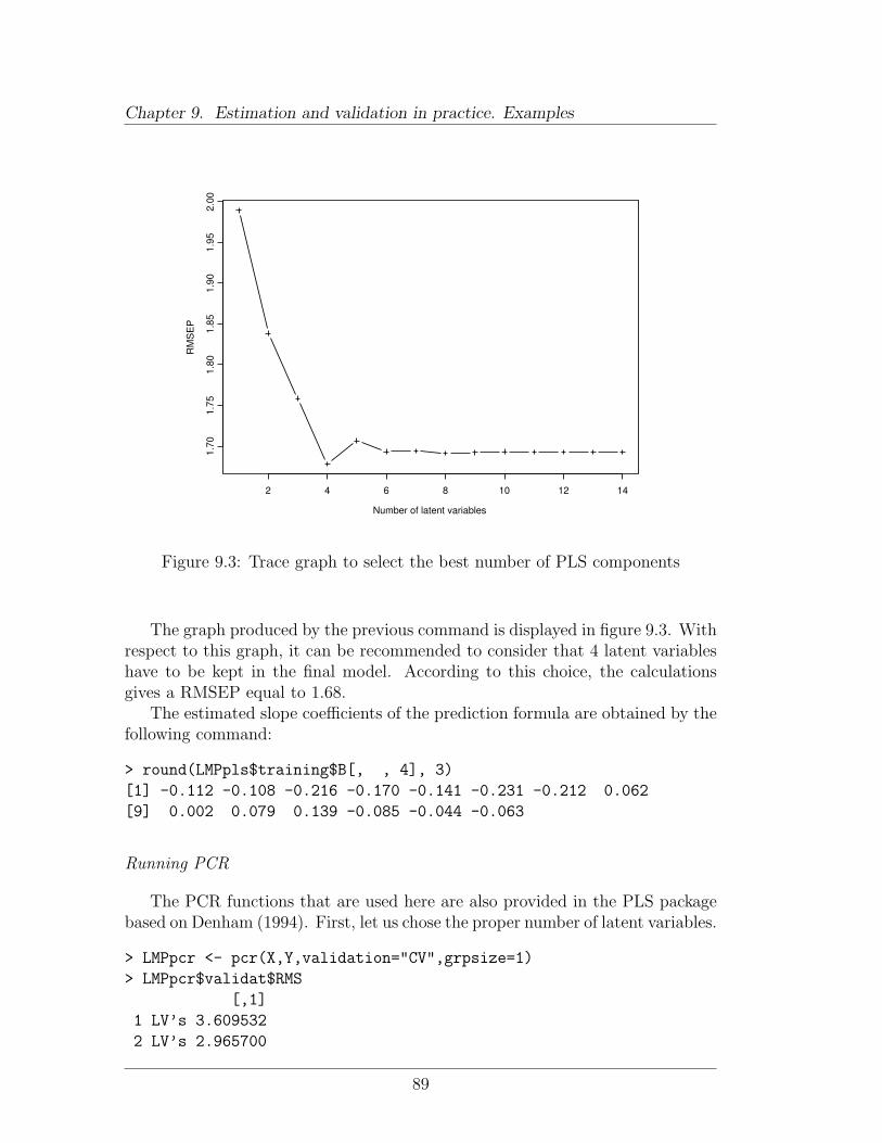
Chapter 9. Estimation and validation in practice. Examples
Number of latent variables
RM
SE
P
2 4 6 8 10 12 14
1.70
1.75
1.80
1.85
1.90
1.95
2.00
Figure 9.3: Trace graph to select the best number of PLS components
The graph produced by the previous command is displayed in figure 9.3. Withrespect to this graph, it can be recommended to consider that 4 latent variableshave to be kept in the final model. According to this choice, the calculationsgives a RMSEP equal to 1.68.
The estimated slope coefficients of the prediction formula are obtained by thefollowing command:
> round(LMPpls$training$B[, , 4], 3)
[1] -0.112 -0.108 -0.216 -0.170 -0.141 -0.231 -0.212 0.062
[9] 0.002 0.079 0.139 -0.085 -0.044 -0.063
Running PCR
The PCR functions that are used here are also provided in the PLS packagebased on Denham (1994). First, let us chose the proper number of latent variables.
> LMPpcr <- pcr(X,Y,validation="CV",grpsize=1)
> LMPpcr$validat$RMS
[,1]
1 LV’s 3.609532
2 LV’s 2.965700
89
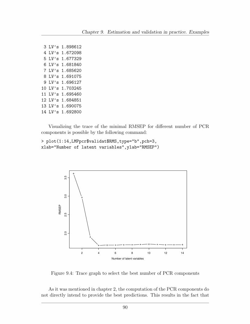
Chapter 9. Estimation and validation in practice. Examples
3 LV’s 1.898612
4 LV’s 1.672098
5 LV’s 1.677329
6 LV’s 1.681840
7 LV’s 1.685620
8 LV’s 1.691075
9 LV’s 1.696127
10 LV’s 1.703245
11 LV’s 1.695460
12 LV’s 1.684851
13 LV’s 1.690075
14 LV’s 1.692800
Visualizing the trace of the minimal RMSEP for different number of PCRcomponents is possible by the following command:
> plot(1:14,LMPpcr$validat$RMS,type="b",pch=3,
xlab="Number of latent variables",ylab="RMSEP")
Number of latent variables
RM
SE
P
2 4 6 8 10 12 14
2.0
2.5
3.0
3.5
Figure 9.4: Trace graph to select the best number of PCR components
As it was mentioned in chapter 2, the computation of the PCR components donot directly intend to provide the best predictions. This results in the fact that
90
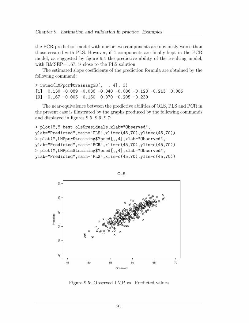
Chapter 9. Estimation and validation in practice. Examples
the PCR prediction model with one or two components are obviously worse thanthose created with PLS. However, if 4 components are finally kept in the PCRmodel, as suggested by figure 9.4 the predictive ability of the resulting model,with RMSEP=1.67, is close to the PLS solution.
The estimated slope coefficients of the prediction formula are obtained by thefollowing command:
> round(LMPpcr$training$B[, , 4], 3)
[1] 0.130 -0.089 -0.036 -0.040 -0.086 -0.123 -0.213 0.086
[9] -0.167 -0.005 -0.150 0.070 -0.205 -0.230
The near-equivalence between the predictive abilities of OLS, PLS and PCR inthe present case is illustrated by the graphs produced by the following commandsand displayed in figures 9.5, 9.6, 9.7:
> plot(Y,Y-best.ols$residuals,xlab="Observed",
ylab="Predicted",main="OLS",xlim=c(45,70),ylim=c(45,70))
> plot(Y,LMPpcr$training$Ypred[,,4],xlab="Observed",
ylab="Predicted",main="PCR",xlim=c(45,70),ylim=c(45,70))
> plot(Y,LMPpls$training$Ypred[,,4],xlab="Observed",
ylab="Predicted",main="PLS",xlim=c(45,70),ylim=c(45,70))
OLS
Observed
Pre
dict
ed
45 50 55 60 65 70
4550
5560
6570
Figure 9.5: Observed LMP vs. Predicted values
91
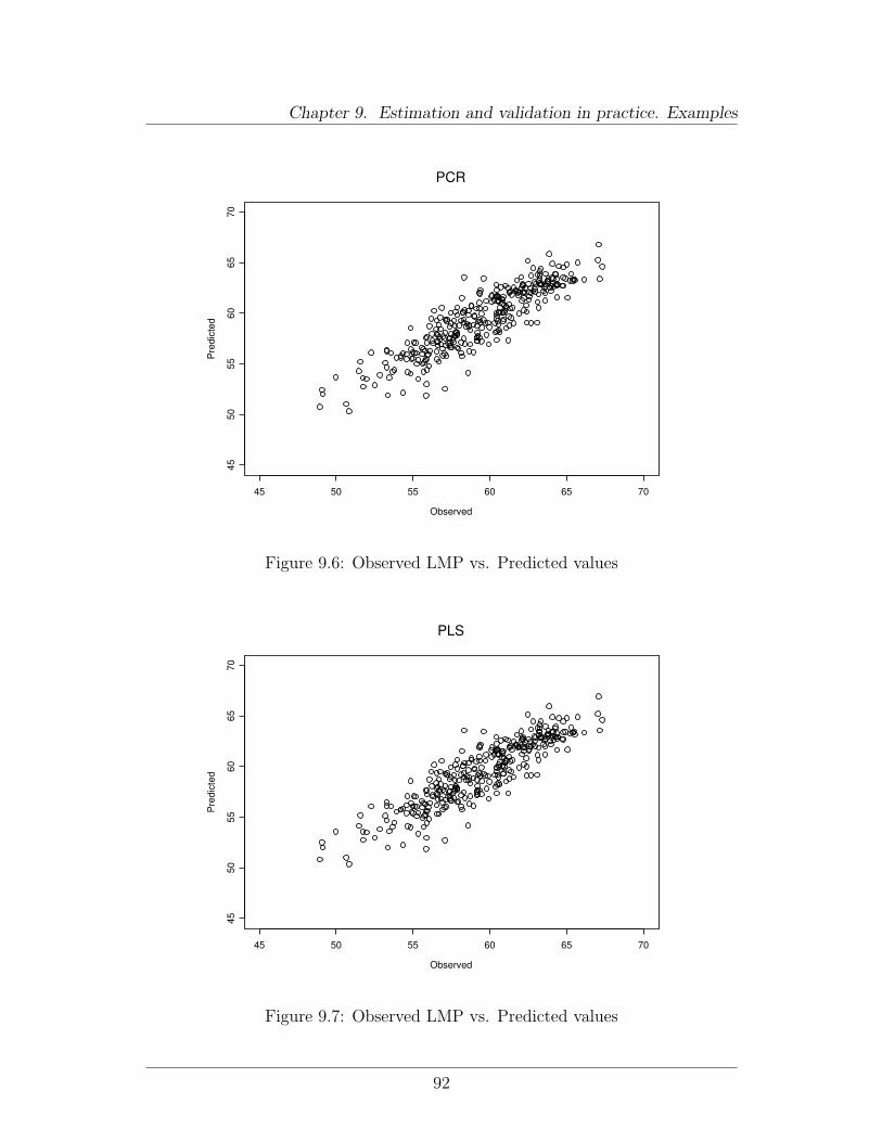
Chapter 9. Estimation and validation in practice. Examples
PCR
Observed
Pre
dict
ed
45 50 55 60 65 70
4550
5560
6570
Figure 9.6: Observed LMP vs. Predicted values
PLS
Observed
Pre
dict
ed
45 50 55 60 65 70
4550
5560
6570
Figure 9.7: Observed LMP vs. Predicted values
92
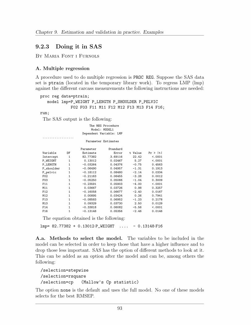
Chapter 9. Estimation and validation in practice. Examples
9.2.3 Doing it in SAS
By Maria Font i Furnols
A. Multiple regression
A procedure used to do multiple regression is PROC REG. Suppose the SAS dataset is ptrain (located in the temporary library work). To regress LMP (lmp)against the different carcass measurements the following instructions are needed:
proc reg data=ptrain;model lmp=P_WEIGHT P_LENGTH P_SHOULDER P_PELVIC
F02 F03 F11 M11 F12 M12 F13 M13 F14 F16;run;
The SAS output is the following:The REG Procedure
Model: MODEL1
Dependent Variable: LMP
..................
Parameter Estimates
Parameter Standard
Variable DF Estimate Error t Value Pr > |t|
Intercept 1 82.77382 3.69116 22.42 <.0001
P_WEIGHT 1 0.13012 0.02467 5.27 <.0001
P_LENGTH 1 -0.03264 0.04376 -0.75 0.4563
P_shoulder 1 -0.06490 0.04957 -1.31 0.1913
P_pelvic 1 -0.18112 0.08480 -2.14 0.0334
F02 1 -0.21163 0.06455 -3.28 0.0012
F03 1 -0.05250 0.05066 -1.04 0.3009
F11 1 -0.23591 0.05903 -4.00 <.0001
M11 1 0.03667 0.03726 0.98 0.3257
F12 1 -0.16058 0.06677 -2.40 0.0167
M12 1 0.00895 0.03424 0.26 0.7941
F13 1 -0.08583 0.06952 -1.23 0.2178
M13 1 0.09329 0.03730 2.50 0.0129
F14 1 -0.33818 0.06082 -5.56 <.0001
F16 1 -0.13148 0.05356 -2.46 0.0146
The equation obtained is the following:
lmp= 82.77382 + 0.13012·P_WEIGHT .... - 0.13148·F16
A.a. Methods to select the model. The variables to be included in themodel can be selected in order to keep those that have a higher influence and todrop those less important. SAS has the option of different methods to look at it.This can be added as an option after the model and can be, among others thefollowing:
/selection=stepwise
/selection=rsquare
/selection=cp (Mallow’s Cp statistic)
The option none is the default and uses the full model. No one of these modelsselects for the best RMSEP.
93
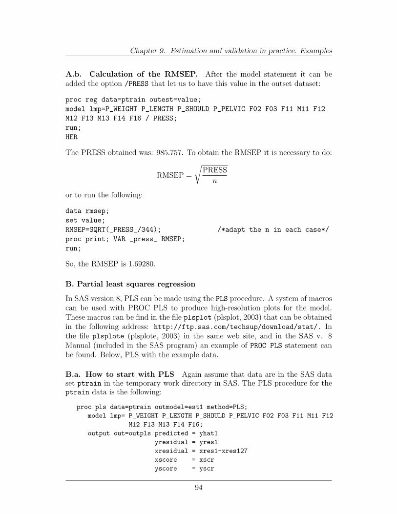
Chapter 9. Estimation and validation in practice. Examples
A.b. Calculation of the RMSEP. After the model statement it can beadded the option /PRESS that let us to have this value in the outset dataset:
proc reg data=ptrain outest=value;
model lmp=P_WEIGHT P_LENGTH P_SHOULD P_PELVIC F02 F03 F11 M11 F12
M12 F13 M13 F14 F16 / PRESS;
run;
HER
The PRESS obtained was: 985.757. To obtain the RMSEP it is necessary to do:
RMSEP =
√PRESS
n
or to run the following:
data rmsep;
set value;
RMSEP=SQRT(_PRESS_/344); /*adapt the n in each case*/
proc print; VAR _press_ RMSEP;
run;
So, the RMSEP is 1.69280.
B. Partial least squares regression
In SAS version 8, PLS can be made using the PLS procedure. A system of macroscan be used with PROC PLS to produce high-resolution plots for the model.These macros can be find in the file plsplot (plsplot, 2003) that can be obtainedin the following address: http://ftp.sas.com/techsup/download/stat/. Inthe file plsplote (plsplote, 2003) in the same web site, and in the SAS v. 8Manual (included in the SAS program) an example of PROC PLS statement canbe found. Below, PLS with the example data.
B.a. How to start with PLS Again assume that data are in the SAS dataset ptrain in the temporary work directory in SAS. The PLS procedure for theptrain data is the following:
proc pls data=ptrain outmodel=est1 method=PLS;model lmp= P_WEIGHT P_LENGTH P_SHOULD P_PELVIC F02 F03 F11 M11 F12
M12 F13 M13 F14 F16;output out=outpls predicted = yhat1
yresidual = yres1xresidual = xres1-xres127xscore = xscryscore = yscr
94
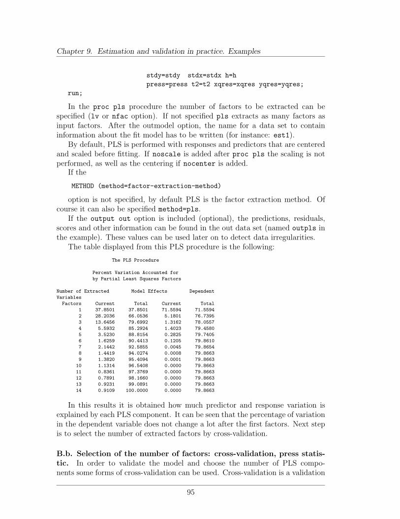
Chapter 9. Estimation and validation in practice. Examples
stdy=stdy stdx=stdx h=hpress=press t2=t2 xqres=xqres yqres=yqres;
run;
In the proc pls procedure the number of factors to be extracted can bespecified (lv or nfac option). If not specified pls extracts as many factors asinput factors. After the outmodel option, the name for a data set to containinformation about the fit model has to be written (for instance: est1).
By default, PLS is performed with responses and predictors that are centeredand scaled before fitting. If noscale is added after proc pls the scaling is notperformed, as well as the centering if nocenter is added.
If the
METHOD (method=factor-extraction-method)
option is not specified, by default PLS is the factor extraction method. Ofcourse it can also be specified method=pls.
If the output out option is included (optional), the predictions, residuals,scores and other information can be found in the out data set (named outpls inthe example). These values can be used later on to detect data irregularities.
The table displayed from this PLS procedure is the following:
The PLS Procedure
Percent Variation Accounted for
by Partial Least Squares Factors
Number of Extracted Model Effects Dependent
Variables
Factors Current Total Current Total
1 37.8501 37.8501 71.5594 71.5594
2 28.2036 66.0536 5.1801 76.7395
3 13.6456 79.6992 1.3162 78.0557
4 5.5932 85.2924 1.4023 79.4580
5 3.5230 88.8154 0.2825 79.7405
6 1.6259 90.4413 0.1205 79.8610
7 2.1442 92.5855 0.0045 79.8654
8 1.4419 94.0274 0.0008 79.8663
9 1.3820 95.4094 0.0001 79.8663
10 1.1314 96.5408 0.0000 79.8663
11 0.8361 97.3769 0.0000 79.8663
12 0.7891 98.1660 0.0000 79.8663
13 0.9231 99.0891 0.0000 79.8663
14 0.9109 100.0000 0.0000 79.8663
In this results it is obtained how much predictor and response variation isexplained by each PLS component. It can be seen that the percentage of variationin the dependent variable does not change a lot after the first factors. Next stepis to select the number of extracted factors by cross-validation.
B.b. Selection of the number of factors: cross-validation, press statis-tic. In order to validate the model and choose the number of PLS compo-nents some forms of cross-validation can be used. Cross-validation is a validation
95
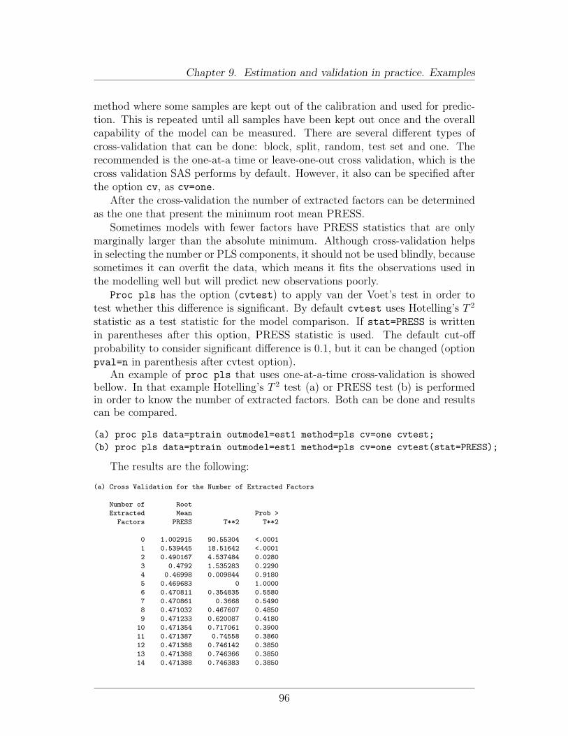
Chapter 9. Estimation and validation in practice. Examples
method where some samples are kept out of the calibration and used for predic-tion. This is repeated until all samples have been kept out once and the overallcapability of the model can be measured. There are several different types ofcross-validation that can be done: block, split, random, test set and one. Therecommended is the one-at-a time or leave-one-out cross validation, which is thecross validation SAS performs by default. However, it also can be specified afterthe option cv, as cv=one.
After the cross-validation the number of extracted factors can be determinedas the one that present the minimum root mean PRESS.
Sometimes models with fewer factors have PRESS statistics that are onlymarginally larger than the absolute minimum. Although cross-validation helpsin selecting the number or PLS components, it should not be used blindly, becausesometimes it can overfit the data, which means it fits the observations used inthe modelling well but will predict new observations poorly.
Proc pls has the option (cvtest) to apply van der Voet’s test in order totest whether this difference is significant. By default cvtest uses Hotelling’s T 2
statistic as a test statistic for the model comparison. If stat=PRESS is writtenin parentheses after this option, PRESS statistic is used. The default cut-offprobability to consider significant difference is 0.1, but it can be changed (optionpval=n in parenthesis after cvtest option).
An example of proc pls that uses one-at-a-time cross-validation is showedbellow. In that example Hotelling’s T 2 test (a) or PRESS test (b) is performedin order to know the number of extracted factors. Both can be done and resultscan be compared.
(a) proc pls data=ptrain outmodel=est1 method=pls cv=one cvtest;(b) proc pls data=ptrain outmodel=est1 method=pls cv=one cvtest(stat=PRESS);
The results are the following:
(a) Cross Validation for the Number of Extracted Factors
Number of Root
Extracted Mean Prob >
Factors PRESS T**2 T**2
0 1.002915 90.55304 <.0001
1 0.539445 18.51642 <.0001
2 0.490167 4.537484 0.0280
3 0.4792 1.535283 0.2290
4 0.46998 0.009844 0.9180
5 0.469683 0 1.0000
6 0.470811 0.354835 0.5580
7 0.470861 0.3668 0.5490
8 0.471032 0.467607 0.4850
9 0.471233 0.620087 0.4180
10 0.471354 0.717061 0.3900
11 0.471387 0.74558 0.3860
12 0.471388 0.746142 0.3850
13 0.471388 0.746366 0.3850
14 0.471388 0.746383 0.3850
96
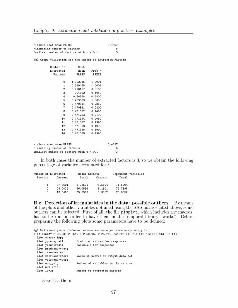
Chapter 9. Estimation and validation in practice. Examples
Minimum root mean PRESS 0.4697
Minimizing number of factors 5
Smallest number of factors with p > 0.1 3
(b) Cross Validation for the Number of Extracted Factors
Number of Root
Extracted Mean Prob >
Factors PRESS PRESS
0 1.002915 <.0001
1 0.539445 <.0001
2 0.490167 0.0130
3 0.4792 0.1050
4 0.46998 0.4800
5 0.469683 1.0000
6 0.470811 0.2850
7 0.470861 0.2800
8 0.471032 0.2490
9 0.471233 0.2190
10 0.471354 0.2050
11 0.471387 0.1990
12 0.471388 0.1990
13 0.471388 0.1990
14 0.471388 0.1990
Minimum root mean PRESS 0.4697
Minimizing number of factors 5
Smallest number of factors with p > 0.1 3
In both cases the number of extracted factors is 3, so we obtain the followingpercentage of variance accounted for :
Number of Extracted Model Effects Dependent Variables
Factors Current Total Current Total
1 37.8501 37.8501 71.5594 71.5594
2 28.2036 66.0536 5.1801 76.7395
3 13.6456 79.6992 1.3162 78.0557
B.c. Detection of irregularities in the data: possible outliers. By meansof the plots and other variables obtained using the SAS macros cited above, someoutliers can be selected. First of all, the file plsplot, which includes the macros,has to be run, in order to have them in the temporal library ”works”. Beforepreparing the following plots some parameters have to be defined:
%global xvars yvars predname resname xscrname yscrname num_x num_y lv;
%let xvars= P_WEIGHT P_LENGTH P_SHOULD P_PELVIC F02 F03 F11 M11 F12 M12 F13 M13 F14 F16;
%let yvars= lmp;
%let ypred=yhat1; Predicted values for responses
%let yres=yres1; Residuals for responses
%let predname=yhat;
%let resname=res;
%let xscrname=xscr; Names of scores in output data set
%let yscrname=yscr;
%let num_y=1; Number of variables in the data set
%let num_x=14;
%let lv=3; Number of extracted factors
as well as the n:
97
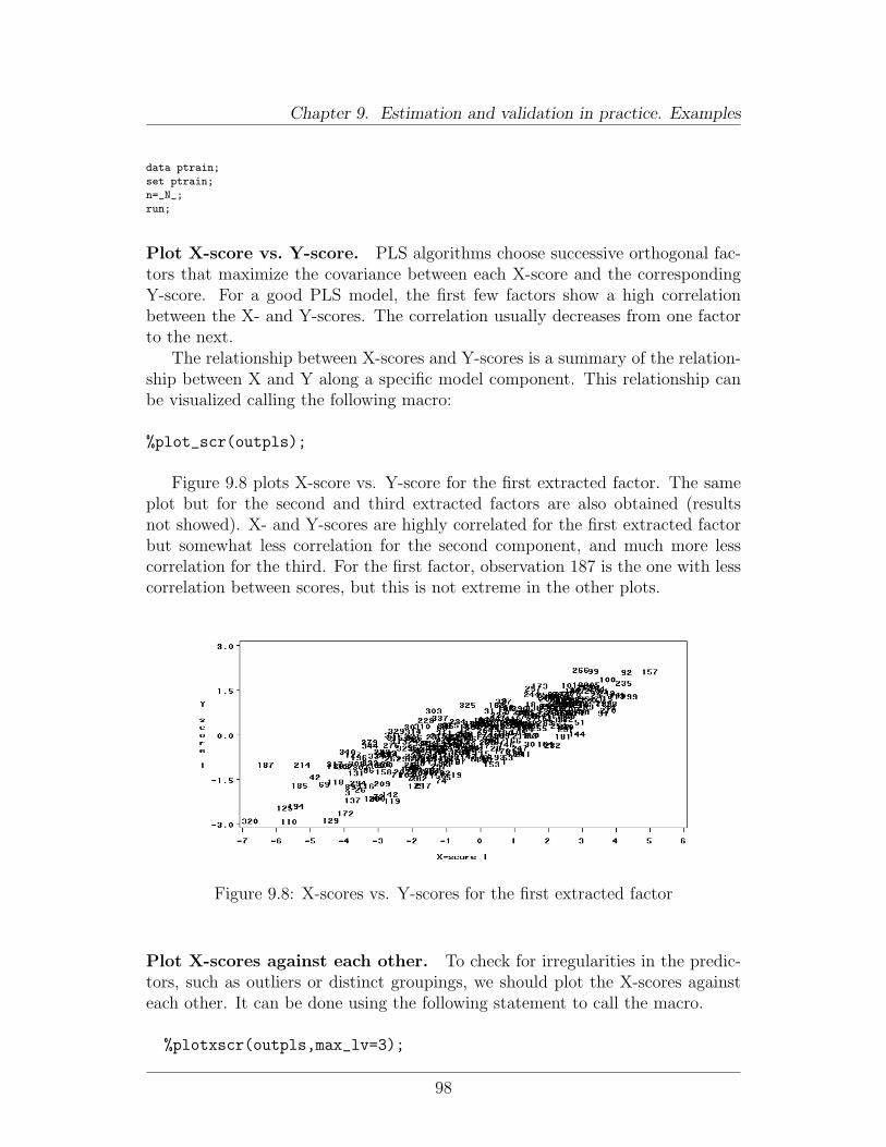
Chapter 9. Estimation and validation in practice. Examples
data ptrain;
set ptrain;
n=_N_;
run;
Plot X-score vs. Y-score. PLS algorithms choose successive orthogonal fac-tors that maximize the covariance between each X-score and the correspondingY-score. For a good PLS model, the first few factors show a high correlationbetween the X- and Y-scores. The correlation usually decreases from one factorto the next.
The relationship between X-scores and Y-scores is a summary of the relation-ship between X and Y along a specific model component. This relationship canbe visualized calling the following macro:
%plot_scr(outpls);
Figure 9.8 plots X-score vs. Y-score for the first extracted factor. The sameplot but for the second and third extracted factors are also obtained (resultsnot showed). X- and Y-scores are highly correlated for the first extracted factorbut somewhat less correlation for the second component, and much more lesscorrelation for the third. For the first factor, observation 187 is the one with lesscorrelation between scores, but this is not extreme in the other plots.
Figure 9.8: X-scores vs. Y-scores for the first extracted factor
Plot X-scores against each other. To check for irregularities in the predic-tors, such as outliers or distinct groupings, we should plot the X-scores againsteach other. It can be done using the following statement to call the macro.
%plotxscr(outpls,max_lv=3);
98
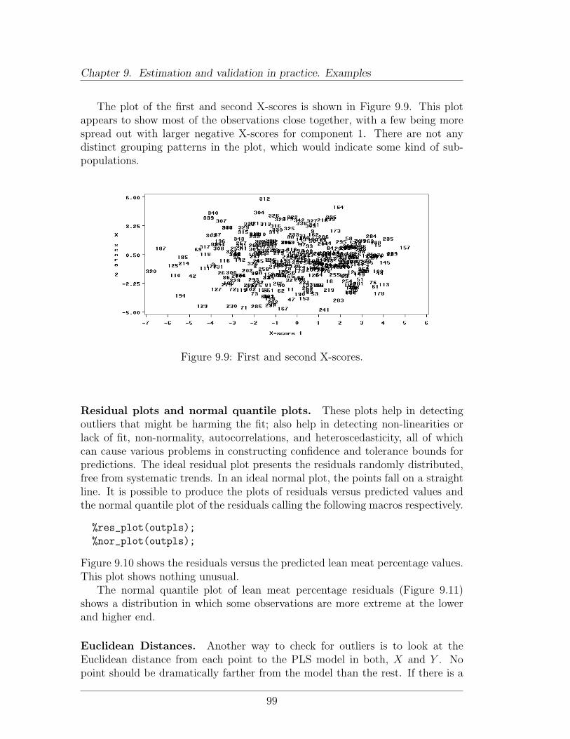
Chapter 9. Estimation and validation in practice. Examples
The plot of the first and second X-scores is shown in Figure 9.9. This plotappears to show most of the observations close together, with a few being morespread out with larger negative X-scores for component 1. There are not anydistinct grouping patterns in the plot, which would indicate some kind of sub-populations.
Figure 9.9: First and second X-scores.
Residual plots and normal quantile plots. These plots help in detectingoutliers that might be harming the fit; also help in detecting non-linearities orlack of fit, non-normality, autocorrelations, and heteroscedasticity, all of whichcan cause various problems in constructing confidence and tolerance bounds forpredictions. The ideal residual plot presents the residuals randomly distributed,free from systematic trends. In an ideal normal plot, the points fall on a straightline. It is possible to produce the plots of residuals versus predicted values andthe normal quantile plot of the residuals calling the following macros respectively.
%res_plot(outpls);
%nor_plot(outpls);
Figure 9.10 shows the residuals versus the predicted lean meat percentage values.This plot shows nothing unusual.
The normal quantile plot of lean meat percentage residuals (Figure 9.11)shows a distribution in which some observations are more extreme at the lowerand higher end.
Euclidean Distances. Another way to check for outliers is to look at theEuclidean distance from each point to the PLS model in both, X and Y . Nopoint should be dramatically farther from the model than the rest. If there is a
99
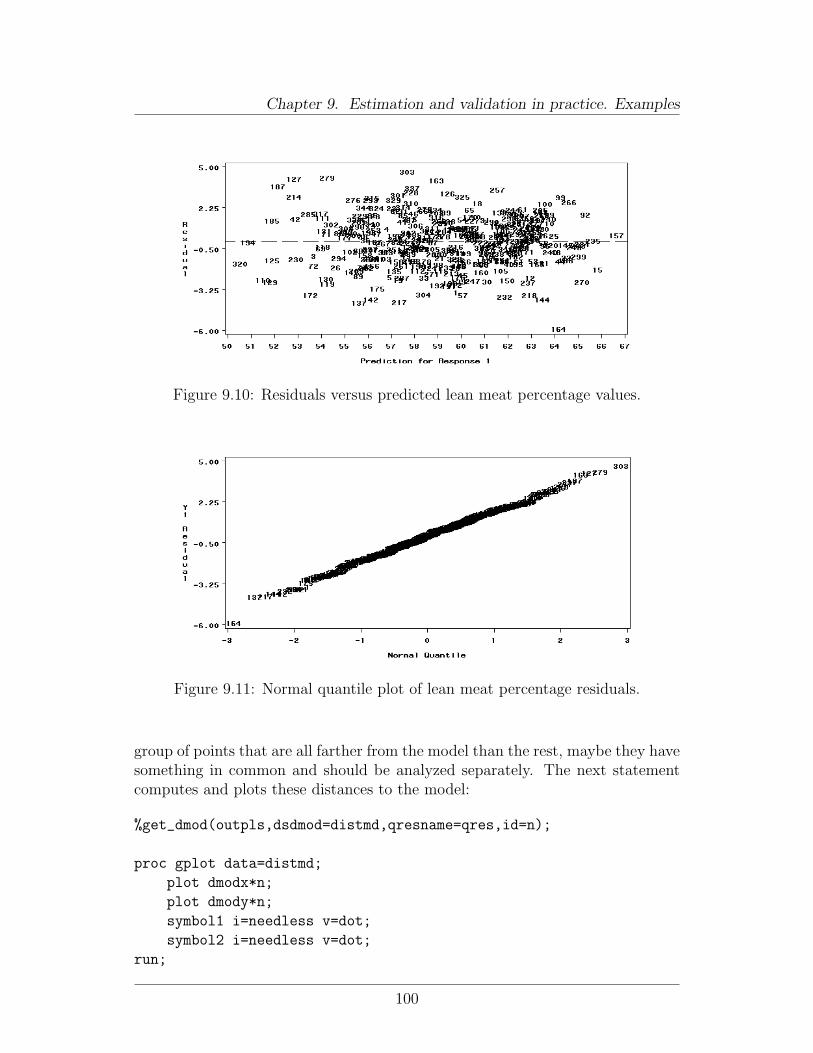
Chapter 9. Estimation and validation in practice. Examples
Figure 9.10: Residuals versus predicted lean meat percentage values.
Figure 9.11: Normal quantile plot of lean meat percentage residuals.
group of points that are all farther from the model than the rest, maybe they havesomething in common and should be analyzed separately. The next statementcomputes and plots these distances to the model:
%get_dmod(outpls,dsdmod=distmd,qresname=qres,id=n);
proc gplot data=distmd;
plot dmodx*n;
plot dmody*n;
symbol1 i=needless v=dot;
symbol2 i=needless v=dot;
run;
100
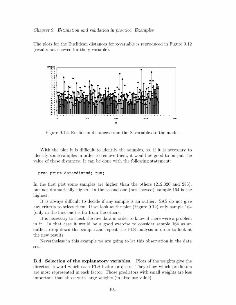
Chapter 9. Estimation and validation in practice. Examples
The plots for the Euclidean distances for x-variable is reproduced in Figure 9.12(results not showed for the y-variable).
Figure 9.12: Euclidean distances from the X-variables to the model.
With the plot it is difficult to identify the samples, so, if it is necessary toidentify some samples in order to remove them, it would be good to output thevalue of these distances. It can be done with the following statement:
proc print data=distmd; run;
In the first plot some samples are higher than the others (212,320 and 285),but not dramatically higher. In the second one (not showed), sample 164 is thehighest.
It is always difficult to decide if any sample is an outlier. SAS do not giveany criteria to select them. If we look at the plot (Figure 9.12) only sample 164(only in the first one) is far from the others.
It is necessary to check the raw data in order to know if there were a problemin it. In that case it would be a good exercise to consider sample 164 as anoutlier, drop down this sample and repeat the PLS analysis in order to look atthe new results.
Nevertheless in this example we are going to let this observation in the dataset.
B.d. Selection of the explanatory variables. Plots of the weights give thedirection toward which each PLS factor projects. They show which predictorsare most represented in each factor. Those predictors with small weights are lessimportant than those with large weights (in absolute value).
101
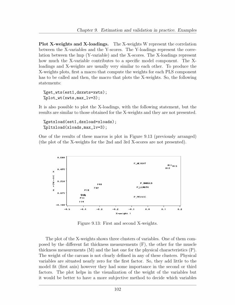
Chapter 9. Estimation and validation in practice. Examples
Plot X-weights and X-loadings. The X-weights W represent the correlationbetween the X-variables and the Y-scores. The Y-loadings represent the corre-lation between the lmp (Y-variable) and the X-scores. The X-loadings representhow much the X-variable contributes to a specific model component. The X-loadings and X-weights are usually very similar to each other. To produce theX-weights plots, first a macro that compute the weights for each PLS componenthas to be called and then, the macro that plots the X-weights. So, the followingstatements:
%get_wts(est1,dsxwts=xwts);
%plot_wt(xwts,max_lv=3);
It is also possible to plot the X-loadings, with the following statement, but theresults are similar to those obtained for the X-weights and they are not presented.
%getxload(est1,dsxload=xloads);
%pltxload(xloads,max_lv=3);
One of the results of these macros is plot in Figure 9.13 (previously arranged)(the plot of the X-weights for the 2nd and 3rd X-scores are not presented).
Figure 9.13: First and second X-weights.
The plot of the X-weights shows three clusters of variables. One of them com-posed by the different fat thickness measurements (F), the other for the musclethickness measurements (M) and the last one for the physical characteristics (P).The weight of the carcass is not clearly defined in any of these clusters. Physicalvariables are situated nearly zero for the first factor. So, they add little to themodel fit (first axis) however they had some importance in the second or thirdfactors. The plot helps in the visualization of the weight of the variables butit would be better to have a more subjective method to decide which variables
102
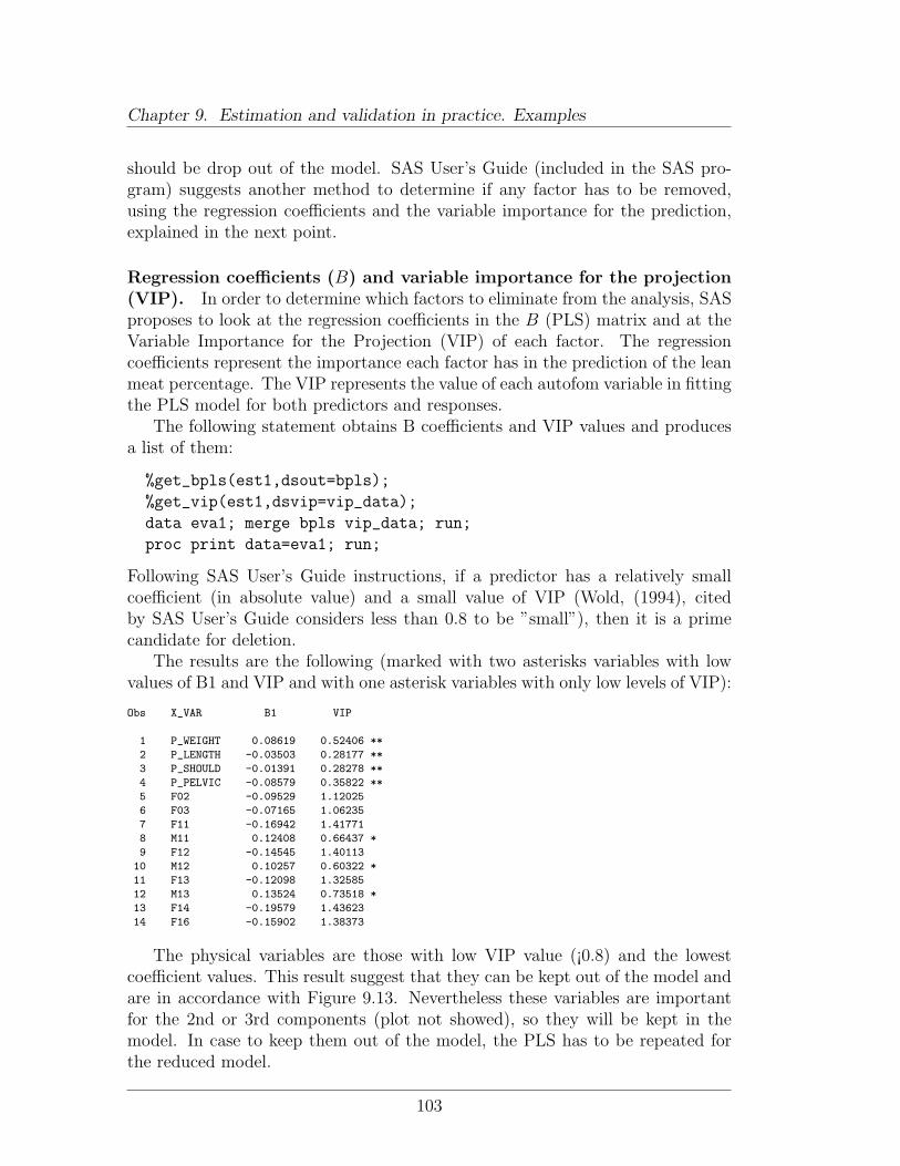
Chapter 9. Estimation and validation in practice. Examples
should be drop out of the model. SAS User’s Guide (included in the SAS pro-gram) suggests another method to determine if any factor has to be removed,using the regression coefficients and the variable importance for the prediction,explained in the next point.
Regression coefficients (B) and variable importance for the projection(VIP). In order to determine which factors to eliminate from the analysis, SASproposes to look at the regression coefficients in the B (PLS) matrix and at theVariable Importance for the Projection (VIP) of each factor. The regressioncoefficients represent the importance each factor has in the prediction of the leanmeat percentage. The VIP represents the value of each autofom variable in fittingthe PLS model for both predictors and responses.
The following statement obtains B coefficients and VIP values and producesa list of them:
%get_bpls(est1,dsout=bpls);
%get_vip(est1,dsvip=vip_data);
data eva1; merge bpls vip_data; run;
proc print data=eva1; run;
Following SAS User’s Guide instructions, if a predictor has a relatively smallcoefficient (in absolute value) and a small value of VIP (Wold, (1994), citedby SAS User’s Guide considers less than 0.8 to be ”small”), then it is a primecandidate for deletion.
The results are the following (marked with two asterisks variables with lowvalues of B1 and VIP and with one asterisk variables with only low levels of VIP):
Obs X_VAR B1 VIP
1 P_WEIGHT 0.08619 0.52406 **
2 P_LENGTH -0.03503 0.28177 **
3 P_SHOULD -0.01391 0.28278 **
4 P_PELVIC -0.08579 0.35822 **
5 F02 -0.09529 1.12025
6 F03 -0.07165 1.06235
7 F11 -0.16942 1.41771
8 M11 0.12408 0.66437 *
9 F12 -0.14545 1.40113
10 M12 0.10257 0.60322 *
11 F13 -0.12098 1.32585
12 M13 0.13524 0.73518 *
13 F14 -0.19579 1.43623
14 F16 -0.15902 1.38373
The physical variables are those with low VIP value (¡0.8) and the lowestcoefficient values. This result suggest that they can be kept out of the model andare in accordance with Figure 9.13. Nevertheless these variables are importantfor the 2nd or 3rd components (plot not showed), so they will be kept in themodel. In case to keep them out of the model, the PLS has to be repeated forthe reduced model.
103
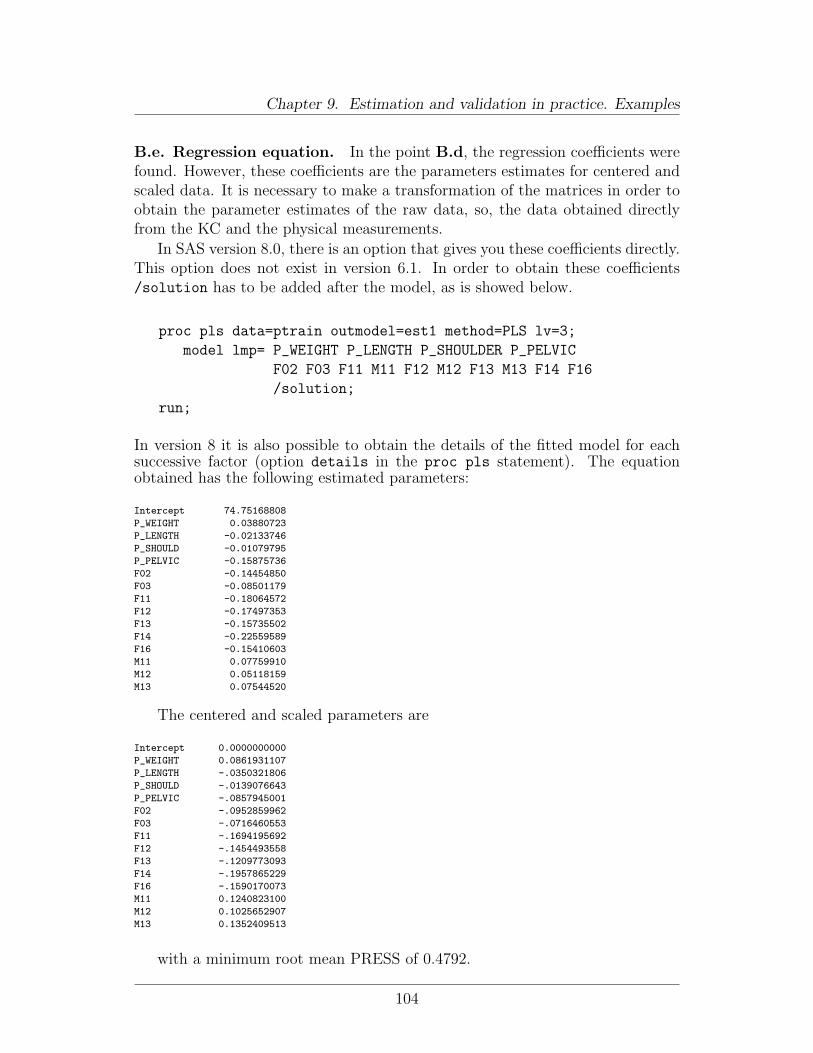
Chapter 9. Estimation and validation in practice. Examples
B.e. Regression equation. In the point B.d, the regression coefficients werefound. However, these coefficients are the parameters estimates for centered andscaled data. It is necessary to make a transformation of the matrices in order toobtain the parameter estimates of the raw data, so, the data obtained directlyfrom the KC and the physical measurements.
In SAS version 8.0, there is an option that gives you these coefficients directly.This option does not exist in version 6.1. In order to obtain these coefficients/solution has to be added after the model, as is showed below.
proc pls data=ptrain outmodel=est1 method=PLS lv=3;
model lmp= P_WEIGHT P_LENGTH P_SHOULDER P_PELVIC
F02 F03 F11 M11 F12 M12 F13 M13 F14 F16
/solution;
run;
In version 8 it is also possible to obtain the details of the fitted model for eachsuccessive factor (option details in the proc pls statement). The equationobtained has the following estimated parameters:
Intercept 74.75168808
P_WEIGHT 0.03880723
P_LENGTH -0.02133746
P_SHOULD -0.01079795
P_PELVIC -0.15875736
F02 -0.14454850
F03 -0.08501179
F11 -0.18064572
F12 -0.17497353
F13 -0.15735502
F14 -0.22559589
F16 -0.15410603
M11 0.07759910
M12 0.05118159
M13 0.07544520
The centered and scaled parameters are
Intercept 0.0000000000
P_WEIGHT 0.0861931107
P_LENGTH -.0350321806
P_SHOULD -.0139076643
P_PELVIC -.0857945001
F02 -.0952859962
F03 -.0716460553
F11 -.1694195692
F12 -.1454493558
F13 -.1209773093
F14 -.1957865229
F16 -.1590170073
M11 0.1240823100
M12 0.1025652907
M13 0.1352409513
with a minimum root mean PRESS of 0.4792.
104
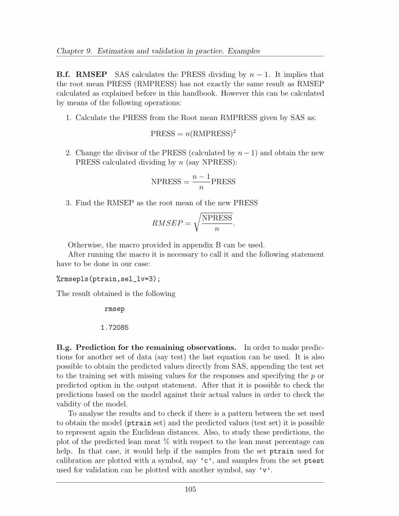
Chapter 9. Estimation and validation in practice. Examples
B.f. RMSEP SAS calculates the PRESS dividing by n − 1. It implies thatthe root mean PRESS (RMPRESS) has not exactly the same result as RMSEPcalculated as explained before in this handbook. However this can be calculatedby means of the following operations:
1. Calculate the PRESS from the Root mean RMPRESS given by SAS as:
PRESS = n(RMPRESS)2
2. Change the divisor of the PRESS (calculated by n− 1) and obtain the newPRESS calculated dividing by n (say NPRESS):
NPRESS =n− 1
nPRESS
3. Find the RMSEP as the root mean of the new PRESS
RMSEP =
√NPRESS
n.
Otherwise, the macro provided in appendix B can be used.After running the macro it is necessary to call it and the following statement
have to be done in our case:
%rmsepls(ptrain,sel_lv=3);
The result obtained is the following
rmsep
1.72085
B.g. Prediction for the remaining observations. In order to make predic-tions for another set of data (say test) the last equation can be used. It is alsopossible to obtain the predicted values directly from SAS, appending the test setto the training set with missing values for the responses and specifying the p orpredicted option in the output statement. After that it is possible to check thepredictions based on the model against their actual values in order to check thevalidity of the model.
To analyse the results and to check if there is a pattern between the set usedto obtain the model (ptrain set) and the predicted values (test set) it is possibleto represent again the Euclidean distances. Also, to study these predictions, theplot of the predicted lean meat % with respect to the lean meat percentage canhelp. In that case, it would help if the samples from the set ptrain used forcalibration are plotted with a symbol, say ’c’, and samples from the set ptest
used for validation can be plotted with another symbol, say ’v’.
105
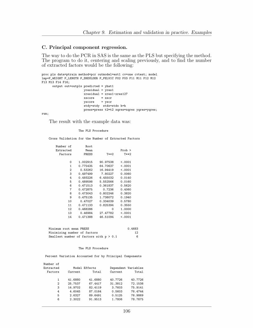
Chapter 9. Estimation and validation in practice. Examples
C. Principal component regression.
The way to do the PCR in SAS is the same as the PLS but specifying the method.The program to do it, centering and scaling previously, and to find the numberof extracted factors would be the following:
proc pls data=ptrain method=pcr outmodel=est1 cv=one cvtest; model
lmp=P_WEIGHT P_LENGTH P_SHOULDER P_PELVIC F02 F03 F11 M11 F12 M12
F13 M13 F14 F16;
output out=outpls predicted = yhat1
yresidual = yres1
xresidual = xres1-xres127
xscore = xscr
yscore = yscr
stdy=stdy stdx=stdx h=h
press=press t2=t2 xqres=xqres yqres=yqres;
run;
The result with the example data was:
The PLS Procedure
Cross Validation for the Number of Extracted Factors
Number of Root
Extracted Mean Prob >
Factors PRESS T**2 T**2
0 1.002915 90.97538 <.0001
1 0.775435 64.70637 <.0001
2 0.53262 16.94419 <.0001
3 0.497499 7.80227 0.0060
4 0.493226 6.455032 0.0140
5 0.489598 5.552566 0.0160
6 0.471513 0.361837 0.5620
7 0.472875 0.7236 0.4060
8 0.473043 0.802246 0.3820
9 0.475135 1.738072 0.1940
10 0.47027 0.334039 0.5780
11 0.471133 0.825394 0.3550
12 0.468286 0 1.0000
13 0.46984 27.47782 <.0001
14 0.471388 46.51094 <.0001
Minimum root mean PRESS 0.4683
Minimizing number of factors 12
Smallest number of factors with p > 0.1 6
The PLS Procedure
Percent Variation Accounted for by Principal Components
Number of
Extracted Model Effects Dependent Variables
Factors Current Total Current Total
1 41.6880 41.6880 40.7726 40.7726
2 25.7537 67.4417 31.3812 72.1538
3 14.9702 82.4119 3.7603 75.9141
4 4.6045 87.0164 0.5603 76.4744
5 2.6327 89.6491 0.5125 76.9869
6 2.3022 91.9513 1.7806 78.7675
106
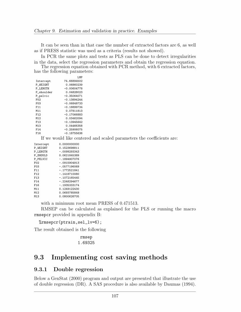
Chapter 9. Estimation and validation in practice. Examples
It can be seen than in that case the number of extracted factors are 6, as wellas if PRESS statistic was used as a criteria (results not showed).
In PCR the same plots and tests as PLS can be done to detect irregularitiesin the data, select the regression parameters and obtain the regression equation.
The regression equation obtained with PCR method, with 6 extracted factors,has the following parameters:
LMP
Intercept 74.66894502
P_WEIGHT 0.06860239
P_LENGTH -0.00604778
P_shoulder 0.04828023
P_pelvic -0.35064071
F02 -0.13894244
F03 -0.06848733
F11 -0.18899734
M11 0.07811813
F12 -0.17066883
M12 0.03462094
F13 -0.13945642
M13 0.04466358
F14 -0.25906075
F16 -0.18755636
If we would like centered and scaled parameters the coefficients are:Intercept 0.0000000000
P_WEIGHT 0.1523698811
P_LENGTH -.0099293343
P_SHOULD 0.0621845389
P_PELVIC -.1894907076
F02 -.0915904913
F03 -.0577196069
F11 -.1772521841
F12 -.1418710080
F13 -.1072165445
F14 -.2248294677
F16 -.1935333174
M11 0.1249122430
M12 0.0693785849
M13 0.0800626705
with a minimum root mean PRESS of 0.471513.RMSEP can be calculated as explained for the PLS or running the macro
rmsepcr provided in appendix B:
%rmsepcr(ptrain,sel_lv=6);
The result obtained is the following
rmsep
1.69325
9.3 Implementing cost saving methods
9.3.1 Double regression
Below a GenStat (2000) program and output are presented that illustrate the useof double regression (DR). A SAS procedure is also available by Daumas (1994).
107
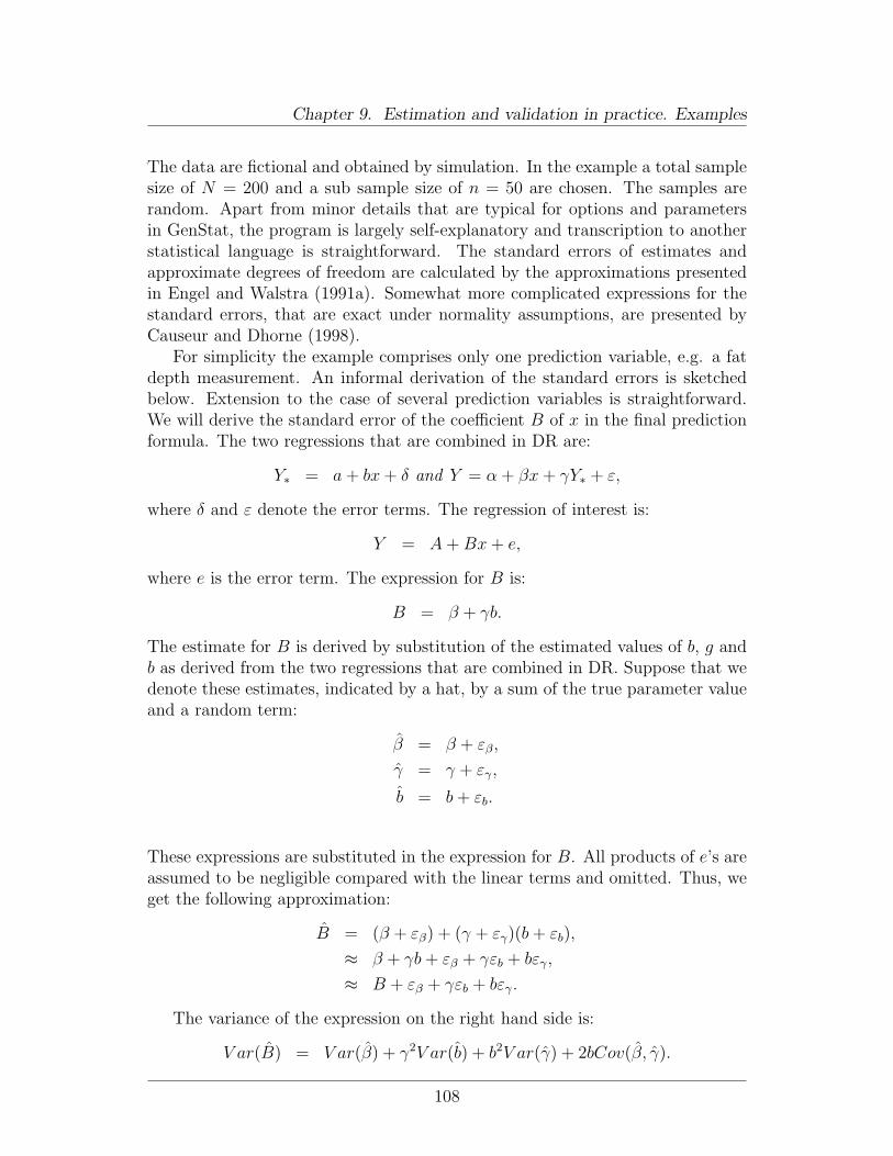
Chapter 9. Estimation and validation in practice. Examples
The data are fictional and obtained by simulation. In the example a total samplesize of N = 200 and a sub sample size of n = 50 are chosen. The samples arerandom. Apart from minor details that are typical for options and parametersin GenStat, the program is largely self-explanatory and transcription to anotherstatistical language is straightforward. The standard errors of estimates andapproximate degrees of freedom are calculated by the approximations presentedin Engel and Walstra (1991a). Somewhat more complicated expressions for thestandard errors, that are exact under normality assumptions, are presented byCauseur and Dhorne (1998).
For simplicity the example comprises only one prediction variable, e.g. a fatdepth measurement. An informal derivation of the standard errors is sketchedbelow. Extension to the case of several prediction variables is straightforward.We will derive the standard error of the coefficient B of x in the final predictionformula. The two regressions that are combined in DR are:
Y∗ = a + bx + δ and Y = α + βx + γY∗ + ε,
where δ and ε denote the error terms. The regression of interest is:
Y = A + Bx + e,
where e is the error term. The expression for B is:
B = β + γb.
The estimate for B is derived by substitution of the estimated values of b, g andb as derived from the two regressions that are combined in DR. Suppose that wedenote these estimates, indicated by a hat, by a sum of the true parameter valueand a random term:
β = β + εβ,
γ = γ + εγ,
b = b + εb.
These expressions are substituted in the expression for B. All products of e’s areassumed to be negligible compared with the linear terms and omitted. Thus, weget the following approximation:
B = (β + εβ) + (γ + εγ)(b + εb),
≈ β + γb + εβ + γεb + bεγ,
≈ B + εβ + γεb + bεγ.
The variance of the expression on the right hand side is:
V ar(B) = V ar(β) + γ2V ar(b) + b2V ar(γ) + 2bCov(β, γ).
108
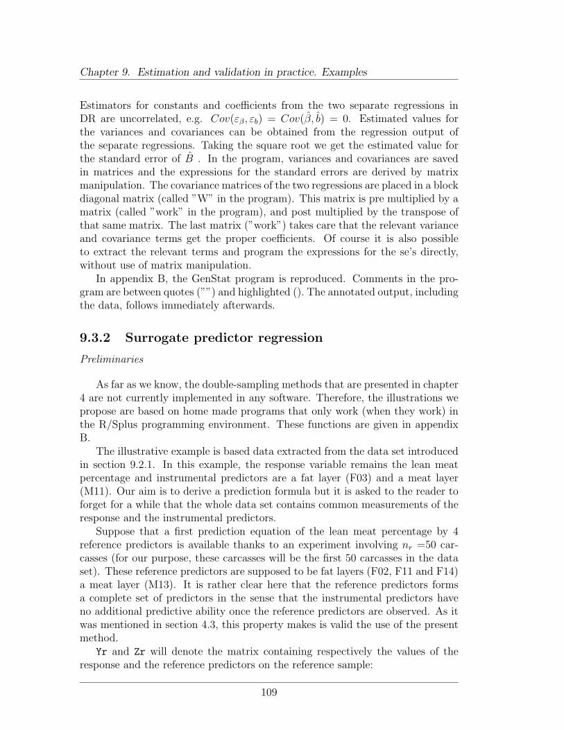
Chapter 9. Estimation and validation in practice. Examples
Estimators for constants and coefficients from the two separate regressions inDR are uncorrelated, e.g. Cov(εβ, εb) = Cov(β, b) = 0. Estimated values forthe variances and covariances can be obtained from the regression output ofthe separate regressions. Taking the square root we get the estimated value forthe standard error of B . In the program, variances and covariances are savedin matrices and the expressions for the standard errors are derived by matrixmanipulation. The covariance matrices of the two regressions are placed in a blockdiagonal matrix (called ”W” in the program). This matrix is pre multiplied by amatrix (called ”work” in the program), and post multiplied by the transpose ofthat same matrix. The last matrix (”work”) takes care that the relevant varianceand covariance terms get the proper coefficients. Of course it is also possibleto extract the relevant terms and program the expressions for the se’s directly,without use of matrix manipulation.
In appendix B, the GenStat program is reproduced. Comments in the pro-gram are between quotes (””) and highlighted (). The annotated output, includingthe data, follows immediately afterwards.
9.3.2 Surrogate predictor regression
Preliminaries
As far as we know, the double-sampling methods that are presented in chapter4 are not currently implemented in any software. Therefore, the illustrations wepropose are based on home made programs that only work (when they work) inthe R/Splus programming environment. These functions are given in appendixB.
The illustrative example is based data extracted from the data set introducedin section 9.2.1. In this example, the response variable remains the lean meatpercentage and instrumental predictors are a fat layer (F03) and a meat layer(M11). Our aim is to derive a prediction formula but it is asked to the reader toforget for a while that the whole data set contains common measurements of theresponse and the instrumental predictors.
Suppose that a first prediction equation of the lean meat percentage by 4reference predictors is available thanks to an experiment involving nr =50 car-casses (for our purpose, these carcasses will be the first 50 carcasses in the dataset). These reference predictors are supposed to be fat layers (F02, F11 and F14)a meat layer (M13). It is rather clear here that the reference predictors formsa complete set of predictors in the sense that the instrumental predictors haveno additional predictive ability once the reference predictors are observed. As itwas mentioned in section 4.3, this property makes is valid the use of the presentmethod.
Yr and Zr will denote the matrix containing respectively the values of theresponse and the reference predictors on the reference sample:
109
Chapter 9. Estimation and validation in practice. Examples
Yr <- Y[1:50]
Zr <- X[1:50,c("F02","F11","F14","M13")]
According to the previous examination of the dimensionality of the instrumentalpredictors in section 9.2, PLS with 2 components is used here to establish thereference prediction formula. The slope coefficients are given by:
> ref.pls <- pls(Zr, Yr)
> sloperef <- ref.pls$training$B[, , 2]
> offsetref <- mean(Yr) - sum(sloperef * apply(Zr, 2, mean))
> coefref <- c(offsetref, sloperef)
> round(coefref, 2)
[1] 65.63 -0.25 -0.41 -0.45 0.18
Deriving a prediction formula for the lean meat percentage by the instrumen-tal predictors will now be achieved through a new experiment consisting only incommon measurements of the reference predictors and the instrumental predic-tors. The first question that has to be addressed is the sample size in this scalingexperiment.
Sampling scheme
Some inputs are of course needed to find a sampling scheme that can ensurethat the EC-requirements are satisfied. More precisely, some prior informationon the variance-covariance of the instrumental and reference predictors is needed.This information can either be obtained by some knowledge from past experi-ments or from a few scaling experiments. Here, it is chosen to get informationsthrough 50 scaling experiments (say the carcasses numbered 51 to 100 in the dataset):
> Zs <- X[51:100, c("F02", "F11", "F14", "M13")]
> Xs <- X[51:100, c("F03", "M11")]
> varzx <- var(cbind(Zs, Xs))
Up to now, the R/Splus object varzx contains the variances and covariances ofboth the reference and the instrumental predictors.
Finally, an estimation of the residual standard deviation of the reference pre-diction equation is necessary. Although the use of PLS does not enable a propercalculation, it will be supposed that the reference residual standard deviationequals about 1.7.
The function optisamp.spr have been written to find the minimum samplesize for the scaling experiment that will provide estimators as efficient as those
110
Chapter 9. Estimation and validation in practice. Examples
that would have been obtained from OLS on a sample of 120 units. The argu-ments of this function are the target sample size n (n = 120 according to theEC-requirements), the reference sample size nr (here nr = 50), the variance-covariance sigmazx of both the reference and the instrumental predictors, thereference residual standard deviation rsdref and the slope coefficients in thereference prediction equation sloperef:
> optisamp.spr(n = 120, nr = 50, sigmazx = varzx, rsdref = 1.7,
sloperef = ref.pls$training$B[, , 2])
[1] 222
It is therefore suggested to run 172 new scaling experiments. It will be supposedthat the scaling sample contains the carcasses numbered 51 to 272:
Zs <- as.matrix(X[51:272,c("F02","F11","F14","M13")])
Xs <- as.matrix(X[51:272,c("F03","M11")])
Suppose just for the illustrative purpose that the cost for a single reference dis-section is 100 and that the cost for a scaling experiment is only 20. The globalcost for such an experiment then equals 50*100+222*20=9440, or equivalently areduction of approximately 22 % relative to the required 120 reference dissections.
Creating the prediction formula
The home made function spr, which arguments are the measurements of theinstrumental predictors Xs and the reference predictors Zs on the scaling sampleand the coefficients coefref of the reference prediction equation, can be used toderive the prediction formula of the lean meat percentage by the instrumentalpredictors:
> spr(Xs, Zs, coefref)
[,1]
60.1831859
F03 -0.7232963
M11 0.1984338
Although it does not validate the present method at all, it can be argued thatthe estimated coefficients would not have been very different if OLS could havebeen performed on the whole data set:
> ls.print(lsfit(X[, c("F03", "M11")], Y))
Residual Standard Error = 2.7348, Multiple R-Square = 0.4251
N = 344, F-statistic = 126.0704 on 2 and 341 df, p-value = 0
111
Chapter 9. Estimation and validation in practice. Examples
coef std.err t.stat p.value
Intercept 59.6111 1.4674 40.6245 0
F03 -0.7188 0.0493 -14.5796 0
M11 0.2197 0.0260 8.4548 0
Validation
First, let us derive the RMSEP for the reference prediction equation:
> rmsep.ref <- pls(Zr, Yr, validation = "CV",
grpsize = 1)$training$RMS[2, 1]
> rmsep.ref
2 LV’s
1.902015
Now the home made function rmsep.spr gives the RMSEP for the predictionformula:
> rmsep.spr(Xs, Zs, sloperef = ref.pls$training$B[, , 2],
rmsepref = rmsep.ref)
[1] 2.997035
At both phase of the sampling scheme, full cross-validation have been used toderive the RMSEPs. According to the content of section 4.3, the resulting RM-SEP is obtained by a combination of the intermediate RMSEPs derived on thereference sample and the scaling sample.
112
Chapter 10
Prospects
By Bas Engel
10.1 Non-linear regression
In classical non-linear regression, it is assumed that
yi = f(xi; a, b, c) + εi,
where f(x; a, b, c) is a function of prediction variable x and some unknown coef-ficients, say a, b and c, which have to be estimated from the data. The mutuallyindependent error terms εi are assumed to have equal variance σ2. Function fis assumed to be non-linear in at least one of the variables a, b or c. Obviously,LR, where f(x; a, b) = a + b ∗ x, is a special case, without non-linear coefficients.
Estimation of a, b and c proceeds analogous to LR by the method of leastsquares. Estimates A, B and C minimise the sum of squares:
n∑i=1
[yi − f(xi; a, b, c)]2 .
The minimum value offers an estimate for σ2:
s2 =n∑
i=1
[yi − f(xi; A, B, C)]2 /d.
Again, d are the degrees of freedom and equal to the sample size n reduced bythe number p of unknowns to be estimated in the formula: d = n − p. Withcoefficients a, b and c: p = 3.
Minimisation of the sum of squares is more complicated than in LR andusually involves some iterative numerical procedure. Least squares estimates A,B and C will be biased estimators for a, b and c. Likewise, s2 will be a biased
113
Chapter 10. Prospects
estimator for σ2. Statistical inference in a non-linear models is mostly basedon large sample theory, even under assumption of normality of error terms εi
few exact small sample results are available for statistical inference. There is noguarantee that the large sample approximations will yield proper results for smallsample sizes. For a sample size of n = 120, estimators may be expected to bewell behaved, e.g. they will be nearly unbiased and they will offer a reasonableimpression of a, b, c and σ2. By way of an RMSE, the estimated residual standarderror s may be evaluated. When inclusion of non-linear terms markedly improvesresults obtained by LR, it seems reasonable to extend the minimum sample sizeof 120 carcasses for LR to classical non-linear regression as well. There is quitesome literature devoted to non-linear regression; we just mention Gallant (1975,1987). There is ample software in most of the larger statistical packages. Theapproach of Engel & Walstra (1993) is actually based on a very specific non-linearmodel. For this particular problem a combination of least squares and non-linearregression, i.e. logistic regression, was used.
10.2 Variance functions
Variance functions have not been used yet in carcass grading. Therefore we willonly supply a few, rather technical, details. When the variance of the error termsis not constant, quite often because it increases with the mean, a logarithmictransformation may stabilise the variance. After logarithmic transformation, anon-linear model may be more appropriate. Note that either with a linear or anon-linear model, after transformation, s2 is not a proper substitute for the RMSEanymore, because it refers to observations log(y) and not to the original observa-tions y. Assuming normality after transformation, the original observations arefollowing a lognormal distribution with the following relationship between theresidual variance V ar(yi) and the mean E(yi) (Mood et al., 1974, p117):
V ar(yi) ={exp(σ2)− 1
}E(yi)
2.
E(yi) will either look like (linear model after transformation):
exp(a + bxi + σ2/2)
or (non-linear model after transformation):
exp[f(xi; a, b, c) + σ2/2
].
Note that back-transformation includes the term σ2/2 in the exponential.Alternatively, we may employ a so called generalized linear model (GLM) (Mc-
Cullagh and Nelder, 1989), specifying a logarithmic link function and a variancefunction of the form:
V ar(yi) = φE(yi)2.
114
Chapter 10. Prospects
Under the assumption of normality of log(y) we have φ = exp(σ2) − 1, andestimation may be performed by least squares on the log-transformed data. Al-ternatively, an estimation procedure called maximum quasi-likelihood (Nelderand Wedderburn, 1972; McCullagh and Nelder, 1989) may be applied to theoriginal data. Maximum quasi-likelihood avoids the need for further distribu-tional assumptions, e.g. no assumption of a (log) normal distribution is needed.Maximum quasi-likelihood is a natural extension of the method of least squaresfor variables y where the variance is a multiple of a known function of the mean(McCullagh, 1983). Standard software for GLMs may be employed to derivemaximum quasi-likelihood estimates.
Note that it may sometimes be appealing to apply a transformation to obtaina linear model. For instance when the theoretical mean is equal to:
E(yi) = b exp(−cxi),
it follows that
log [E(yi)] = log(b)− cxi.
The latter expression is linear in log(b) and c. Obviously, when the variancewas constant before transformation, it will not be constant after transformation.In that case, a GLM with a logarithmic link function and a constant variancefunction could be employed. This is a special case of the classical non-linearregression model with all the non-linearity concentrated in the logarithmic linkfunction.
Both for least squares after log-transformation and maximum quasi-likelihoodwith a (quadratic) variance function, it is not immediately apparent what a suit-able substitute for the RMSE should be. The problem is that the RMSE willdepend on the prediction variable x through the mean E(y). Evaluation of themaximum RMSE over a suitable range of x-values seems to be an acceptableapproach.
115


Chapter 11
Reporting to the Commission -results of the trial
By Gerard Daumas
The present EU regulation lays out:“Part two of the protocol should give a detailed description of the results of
the dissection trial and include in particular:
1. a presentation of the statistical methods used in relation to the samplingmethod chosen,
2. the equation which will be introduced or amended,
3. a numerical and a graphic description of the results,
4. a description of the new apparatus,
5. the weight limit of the pigs for which the new method may be used and anyother limitation in relation to the practical use of the method.”
These items have not been specifically discussed. Nevertheless, one can lookfor the following items at the corresponding sections:
• Item 1: see chapters 2 and 4.
• Item 3: see chapters 8 and 9.
117

Appendix A
References
Causeur, D. (2003) Optimal sampling from concomitant variables for regressionproblems. J. Stat. Plan. and Inf. To appear.Causeur, D. and Dhorne, T. (1998) Finite sample properties of a multivariateextension of double regression. Biometrics 54 1591-1601.Causeur, D. and Dhorne, T. (2003) Linear Regression Models under Condi-tional Independence Restrictions. Scand. J. Statist 30, 637 - 650.Cochran, W.G. (1977). Sampling Techniques. 3rd edition, New York: Wiley.Cook, G.L. and Yates, C.M. (1992). A report to the Commission of theEuropean Communities on Research concerning the harmonization of methodsfor grading pig carcasses in the Community.Daumas, G (1994). La double regression sous SAS. Lettre d’information SASACTA, 23.Daumas, G. (2003). A description of the European slaughterpig populationsand their classification. EUPIGCLASS report, 42 p.Daumas, G., Causeur, D., Dhorne, T., Schollhammer, E. (1998). Thenew pig carcass grading methods in France. Proceedings 44th ICoMST, Barcelona(Spain), C-64, 948-949.Daumas, G. and Dhorne, T. (1995). French protocol for updating of pigcarcasses classification methods in 1996 - 1st part - EC Working document.Daumas, G. and Dhorne, T. (1997). The lean meat content of pig carcasses:determination and estimation. French Swine Research Days, 29, 171-180.Daumas, G. and Dhorne, T. (1998). Pig carcass grading in European Union.Proceedings of 44th ICoMST, Barcelona, Spain. C-63, 946-947.Daumas, G., Dhorne, T., Gispert, M. (1994). Accounting for the sex effecton prediction of pig carcass lean meat percentage in the Community. Proc. 40thICoMST, La Haye (The Netherlands), S III. 11, 9 pp.Denham, M.C. (1995) Implementing Partial Least Squares. Statistics andComputing 5, 191-202.Dhorne, T.J. (2000). Contribution to EUPIGCLASS workshop, Lelystad, TheNetherlands.
119
Chapter A. References
Draper, N.R., Smith, H. (1981). Applied regression analysis. 2nd edition.New York: John Wiley.Engel, B. (1987). Increasing precision or reducing expense in regression exper-iments by using information from a concomitant variable. GLW research reportLWA-87-1, Wageningen, The Netherlands.Engel, B. and Walstra, P. (1991a) Increasing precision or reducing expense inregression experiments by using information from a concomitant variable. Bio-metrics 47 1011-1023.Engel, B and Walstra, P. (1991b) A simple method to increase precision orreduce expense in regression experiments to predict the proportion of lean meatof carcasses. Animal production 53 353-359.Engel, B., Walstra, P. (1993). Accounting for subpopulations in prediction ofthe proportion of lean meat of pig carcasses. Animal Production 57: 147-152.Engel, B., Buist, W.G., Walstra, P., Olsen, E., Daumas, G. (2003a).Accuracy of prediction of percentage lean meat and authorization of carcass mea-surement instruments: adverse effects of incorrect sampling of carcasses in pigclassification. Animal Science 76: 199-209.Engel, B., Buist, W.G., Font I Furnols, M., Lambooij, E. (2003b). Sub-populations and accuracy of prediction in pig carcass classification. Animal Sci-ence, in press.European Community (1994a) EC regulation No. 3127/94, amending reg-ulation (EC) No 2967/85 laying down detailed rules for the application of thecommunity scale for grading pig carcasses.European Community (1994b) Commission Decision amendment to the deci-sion authorizing methods for grading pig carcasses in Spain (94/337/EEC).Feinberg, M. (1995). Basics of interlaboratory studies: the trends in the newISO 5725 standard edition. Trends in analytical chemistry, vol. 14, no.9, Paris.Font i Furnols, M. (2002). Contribution to EUPIGCLASS meeting, Gent,Belgium.Gallant, A.R. (1975). Nonlinear regression. The American Statistician 29:73-81.Gallant, A.R. (1987). Nonlinear Statistical Models. New York: John Wiley.Gispert, M., Dhorne, T., Diestre A., Daumas, G., (1996). Efecto del sexoen la prediccion del contenido en magro de la canal porcina en Espana, Franciay Paıses Bajos. Invest. Agr. : Prod. Sanid. Anim. Vol. 11 (1), 1996.Helland, I.S. (1998) Model reduction for prediction in regression models. Scand.J. Statist 27, 1-20.ISO 5725 (1994). Accuracy (trueness and precision) of measurement methodsand results.Mc Ardle, J. (1987). LVPLS Ver. 1.8. Downloadable freely atftp://kiptron.psyc.virginia.edu/pub/lvpls.McCullagh, P., Nelder, J.A. (1989), Generalized linear models. 2nd edition.London: Chapman and Hall.
120
Chapter A. References
McCullagh, P. (1991), Quasi-likelihood and estimating functions. Ch. 11 of:Statistical theory and modelling. In honour of Sir David Cox, FRS. Edited by:D.V.Hinkley, N. Reid and E.J.Snell. London: Chapman and Hall.Mood, A.M., Graybill, F.A. and Boes, D.C. (1963). Introduction to thetheory of statistics. 3rd edition. Tokyo: McGraw-Hill.Montgomery, D.C., Peck, E.A. (1992). Introduction to linear regressionanalysis. 2nd edition. New York: John Wiley.Naes, T., Irgens, C., Martens, H. (1986). Comparison of linear statisticalmethods for calibration of NIR instruments. Applied Statistics 35: 195-206.Nelder, J.A., Wedderburn, R.W.M. (1972). Generalized linear models.Journal of the Royal Statistical Society A 135: 370-384.Olsen, E.V. (1997). Accuracy of industrial methods for meat quality measure-ments. Congress Proceedings, 43rd ICOMST.Plsplot (2003). Consulted in http://ftp.sas.com/techsup/download/stat/ in Ju-ly 2003.Plsplote (2003). Consulted in http://ftp.sas.com/techsup/download/stat/ inJuly 2003.Rao, C.R. and Toutenburg, H. (1999) Linear Models : Least Squares andAlternatives. 2nd Edition. Springer Verlag Ed.Rousseuw, P. and Leroy, A. (1987) Robust Regression and Outlier Detection.John Wiley & and sons eds.Scheper J. and Scholz W. (1985). DLG-Schnittfuhrung fur die Zerlegung derSchlachtkorper von Rind, Kalb, Schwein und Schaf. Arbeitsunterlagen DLG.Sundberg, R. (1999) Multivariate calibrationdirect and indirect regression me-thodology (with discussion). Scand. J. Statist 26, 161-207.Tille, Y. (2001). Theorie des sondages : echantillonnage et estimation en pop-ulations finies. Paris. Dunod. 284 p.Tobias, R.D. (1997a) An Introduction to Partial Least Squares Regression.(http://ftp.sas.com/techsup/download/technote/ts509.pdf) TS-509, SAS Insti-tute Inc., Cary, N.C.(see also http://support.sas.com/techsup/faq/stat proc/plsproc.html)Tobias, R.D. (1997b) Examples Using the PLS Procedure.(http://support.sas.com/rnd/app/papers/plsex.pdf)SAS Institute Inc., Cary, N.C.Walstra, P. (1980). Growth and carcass composition from birth to maturity inrelation to feeding level and sex in Dutch Landrace pigs. PhD-thesis. Mededelin-gen, Landbouwhogeschool Wageningen, 80-4.Walstra, P. (1986). Assessment of the regression formula for estimation of thelean percentage by HGP-measurements in The Netherlands. EC-working paper,Brussels, VI/4849/86.Walstra, P., Merkus, G.S.M. (1995). Procedure for assessment of the leanmeat percentage as a consequence of the new EC reference dissection method inpig carcass classification. Unpublished document ID-Lelystad, The Netherlands.
121

Chapter A. References
Walstra, P. and Merkus, G.S.M. (1996). Procedure for assessment of thelean meat percentage as a consequence of the new EU reference dissection methodin pig carcass classification. Report ID-DLO 96.014, March, 22 pp.
122

Appendix B
Technical details
B.1 SAS Macros for PLS and PCR
/definition of the data/
%global xvars yvars ;
%let xvars= P_WEIGHT P_LENGTH P_SHOULDER P_PELVIC F02 F03 F11 M11 F12 M12 F13 M13 F14 F16;
%let yvars=lmp;
/macro to calculate the different RMSEP with leave one out/
Variables required to be defined: dades=name of the data set
(without missing values)
%macro rmsep(dades);
data regre; set &dades(keep= &xvars &yvars );
call symput(’num_x’,_N_);run;
%do i=1 %to &num_x;
data regres; set regre; if _N_=&i then &yvars=.; proc reg
noprint; model &yvars=&xvars/p; output out=tt&i
p=yhat;
run;
%end;
%do i=1 %to &num_x;
data rr&i; merge tt&i &dades; if _N_=&i;
ysqu=(&yvars-yhat)*(&yvars-yhat); run; data kk&i; set rr&i
(keep=ysqu); run;
%end;
%do i=1 %to 1;
data mitja&i; set kk&i; run;
%end;
%do i=2 %to &num_x;
data mitja&i;
%let j=%eval(&i-1);
set kk&i mitja&j; run;
%end;
%do i=&num_x %to &num_x;
proc means data=mitja&i noprint; output out=mitjana; run;
%end;
data result; set mitjana; if _STAT_=’MEAN’ ; rmsep=(YSQU)**0.5;
proc print noobs; var rmsep; run;
%mend rmsep;
/definition of the variables/
%global xvars yvars ypred;
%let xvars= P_WEIGHT P_LENGTH P_SHOULD P_PELVIC F02 F03 F11 M11 F12 M12 F13 M13 F14 F16;
%let yvars= lmp;
123

Chapter B. Technical details
%let predicted=yhat1;
/macro to calculate RMSEP for PLS/ Variables required to be
defined:
dades= name of the data set and should not contain missing values
sel_lv= number of factors to take into consideration
%macro rmsepls(dades,sel_lv=&lv);
data pls1; set &dades(keep= &xvars &yvars );
call symput(’num_x’,_N_);run;
%do i=1 %to &num_x;
data pls2; set pls1; if _N_=&i then &yvars=.; proc pls method=pls
lv=&sel_lv noprint ; model &yvars=&xvars; output out=tt&i
predicted=yhat1 ; run;
%end;
%do i=1 %to &num_x;
data rr&i; merge tt&i &dades ; if _N_=&i;
ysqu=(&yvars-yhat1)*(&yvars-yhat1); run; data kk&i; set rr&i
(keep=ysqu); run;
%end;
%do i=1 %to 1;
data mitja&i; set kk&i; run;
%end;
%do i=2 %to &num_x;
data mitja&i;
%let j=%eval(&i-1);
set kk&i mitja&j; run;
%end;
%do i=&num_x %to &num_x;
proc means data=mitja&i noprint; output out=mitjana; run;
%end;
data result; set mitjana; if _STAT_=’MEAN’ ; rmsep=(YSQU)**0.5;
proc print noobs; var rmsep; run;
%mend rmsepls;
/definition of the variables/
%global xvars yvars ypred;
%let xvars= P_WEIGHT P_LENGTH P_SHOULD P_PELVIC F02 F03 F11 M11 F12 M12 F13 M13 F14 F16;
%let yvars= lmp;
%let predicted=yhat1;
/macro to calculate RMSEP for PCR/ Variables required to be
defined:
dades= name of the data set and should not contain missing values
sel_lv= number of factors to take into consideration
%macro rmsepcr(dades,sel_lv=&lv);
data pcr1; set &dades(keep= &xvars &yvars );
call symput(’num_x’,_N_);run;
%do i=1 %to &num_x;
data pcr2; set pcr1; if _N_=&i then &yvars=.; proc pls method=pcr
lv=&sel_lv noprint ; model &yvars=&xvars; output out=tt&i
predicted=yhat1 ; run;
%end;
%do i=1 %to &num_x;
data rr&i; merge tt&i &dades ; if _N_=&i;
ysqu=(&yvars-yhat1)*(&yvars-yhat1); run; data kk&i; set rr&i
(keep=ysqu); run;
%end;
%do i=1 %to 1;
data mitja&i; set kk&i; run;
%end;
%do i=2 %to &num_x;
data mitja&i;
%let j=%eval(&i-1);
124
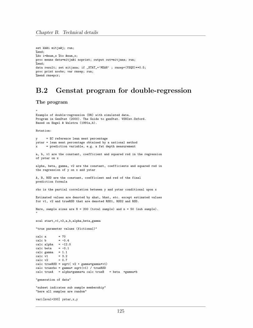
Chapter B. Technical details
set kk&i mitja&j; run;
%end;
%do i=&num_x %to &num_x;
proc means data=mitja&i noprint; output out=mitjana; run;
%end;
data result; set mitjana; if _STAT_=’MEAN’ ; rmsep=(YSQU)**0.5;
proc print noobs; var rmsep; run;
%mend rmsepcr;
B.2 Genstat program for double-regression
The program
"
Example of double-regression (DR) with simulated data.
Program in GenStat (2000). The Guide to genStat. VSNInt.Oxford.
Based on Engel & Walstra (1991a,b).
Notation:
y = EC reference lean meat percentage
ystar = lean meat percentage obtained by a national method
x = prediction variable, e.g. a fat depth measurement
a, b, v1 are the constant, coefficient and squared rsd in the regression
of ystar on x
alpha, beta, gamma, v2 are the constant, coefficients and squared rsd in
the regression of y on x and ystar
A, B, RSD are the constant, coefficient and rsd of the final
prediction formula
rho is the partial correlation between y and ystar conditional upon x
Estimated values are denoted by ahat, bhat, etc. except estimated values
for v1, v2 and trueRSD that are denoted RSD1, RSD2 and RSD.
Here, sample sizes are N = 200 (total sample) and n = 50 (sub sample).
"
scal start,v1,v2,a,b,alpha,beta,gamma
"true parameter values (fictional)"
calc a = 70
calc b = -0.4
calc alpha = -12.0
calc beta = -0.1
calc gamma = 1.1
calc v1 = 3.2
calc v2 = 0.7
calc trueRSD = sqrt( v2 + gamma*gamma*v1)
calc truerho = gamma* sqrt(v1) / trueRSD
calc trueA = alpha+gamma*a calc trueB = beta +gamma*b
"generation of data"
"subset indicates sub sample membership"
"here all samples are random"
vari[nval=200] ystar,x,y
125
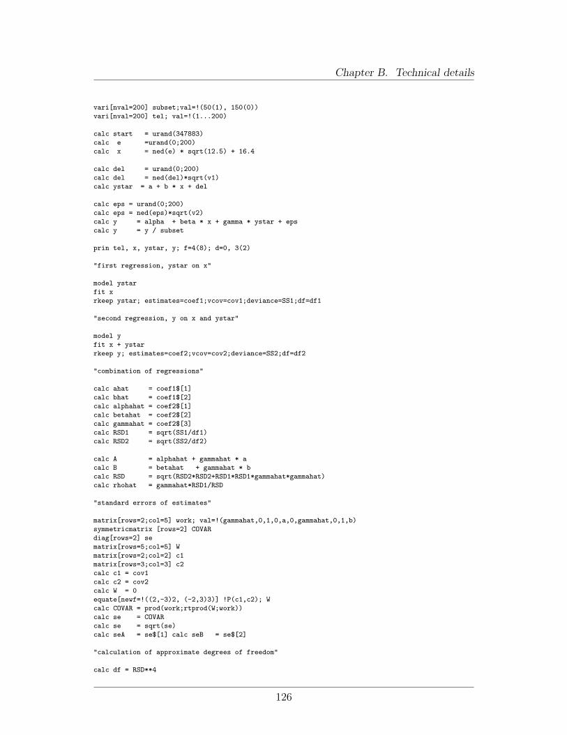
Chapter B. Technical details
vari[nval=200] subset;val=!(50(1), 150(0))
vari[nval=200] tel; val=!(1...200)
calc start = urand(347883)
calc e =urand(0;200)
calc x = ned(e) * sqrt(12.5) + 16.4
calc del = urand(0;200)
calc del = ned(del)*sqrt(v1)
calc ystar = a + b * x + del
calc eps = urand(0;200)
calc eps = ned(eps)*sqrt(v2)
calc y = alpha + beta * x + gamma * ystar + eps
calc y = y / subset
prin tel, x, ystar, y; f=4(8); d=0, 3(2)
"first regression, ystar on x"
model ystar
fit x
rkeep ystar; estimates=coef1;vcov=cov1;deviance=SS1;df=df1
"second regression, y on x and ystar"
model y
fit x + ystar
rkeep y; estimates=coef2;vcov=cov2;deviance=SS2;df=df2
"combination of regressions"
calc ahat = coef1$[1]
calc bhat = coef1$[2]
calc alphahat = coef2$[1]
calc betahat = coef2$[2]
calc gammahat = coef2$[3]
calc RSD1 = sqrt(SS1/df1)
calc RSD2 = sqrt(SS2/df2)
calc A = alphahat + gammahat * a
calc B = betahat + gammahat * b
calc RSD = sqrt(RSD2*RSD2+RSD1*RSD1*gammahat*gammahat)
calc rhohat = gammahat*RSD1/RSD
"standard errors of estimates"
matrix[rows=2;col=5] work; val=!(gammahat,0,1,0,a,0,gammahat,0,1,b)
symmetricmatrix [rows=2] COVAR
diag[rows=2] se
matrix[rows=5;col=5] W
matrix[rows=2;col=2] c1
matrix[rows=3;col=3] c2
calc c1 = cov1
calc c2 = cov2
calc W = 0
equate[newf=!((2,-3)2, (-2,3)3)] !P(c1,c2); W
calc COVAR = prod(work;rtprod(W;work))
calc se = COVAR
calc se = sqrt(se)
calc seA = se$[1] calc seB = se$[2]
"calculation of approximate degrees of freedom"
calc df = RSD**4
126
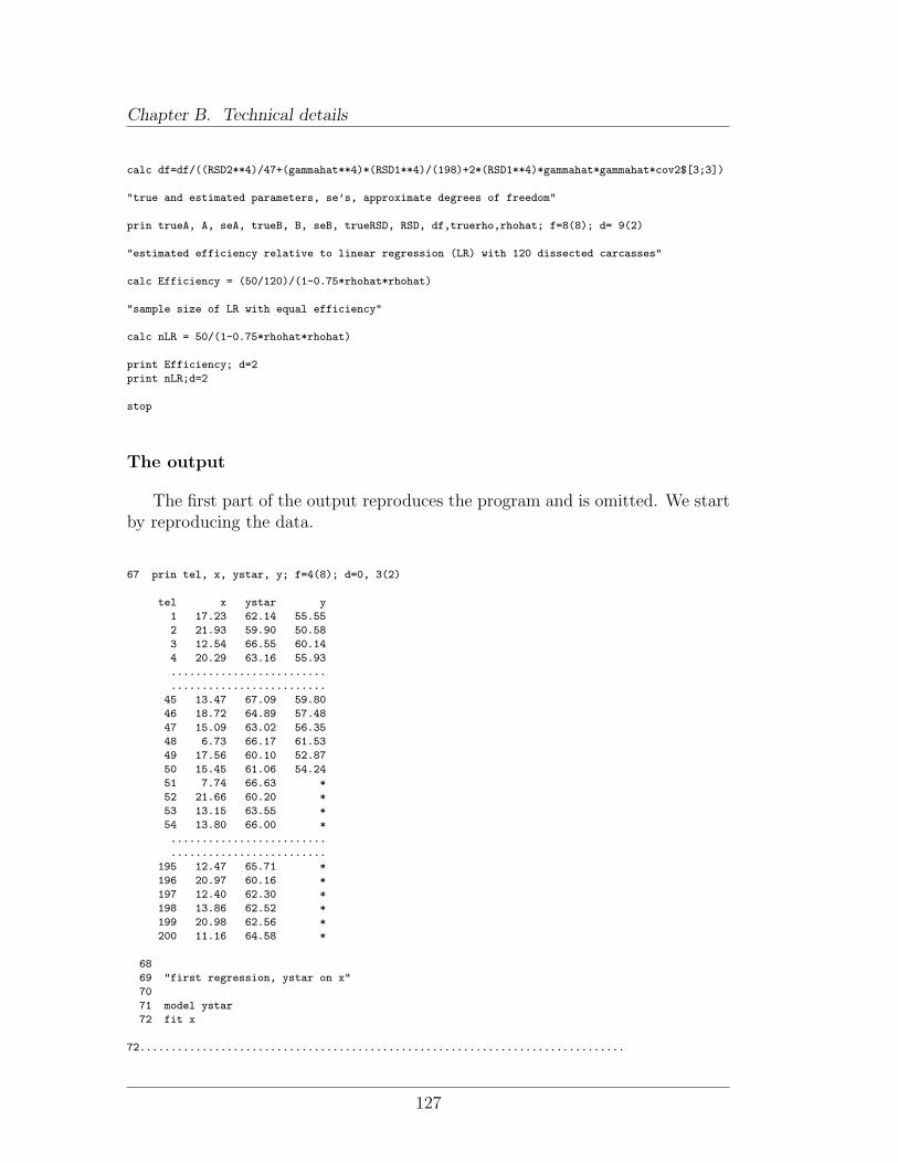
Chapter B. Technical details
calc df=df/((RSD2**4)/47+(gammahat**4)*(RSD1**4)/(198)+2*(RSD1**4)*gammahat*gammahat*cov2$[3;3])
"true and estimated parameters, se’s, approximate degrees of freedom"
prin trueA, A, seA, trueB, B, seB, trueRSD, RSD, df,truerho,rhohat; f=8(8); d= 9(2)
"estimated efficiency relative to linear regression (LR) with 120 dissected carcasses"
calc Efficiency = (50/120)/(1-0.75*rhohat*rhohat)
"sample size of LR with equal efficiency"
calc nLR = 50/(1-0.75*rhohat*rhohat)
print Efficiency; d=2
print nLR;d=2
stop
The output
The first part of the output reproduces the program and is omitted. We startby reproducing the data.
67 prin tel, x, ystar, y; f=4(8); d=0, 3(2)
tel x ystar y
1 17.23 62.14 55.55
2 21.93 59.90 50.58
3 12.54 66.55 60.14
4 20.29 63.16 55.93
.........................
.........................
45 13.47 67.09 59.80
46 18.72 64.89 57.48
47 15.09 63.02 56.35
48 6.73 66.17 61.53
49 17.56 60.10 52.87
50 15.45 61.06 54.24
51 7.74 66.63 *
52 21.66 60.20 *
53 13.15 63.55 *
54 13.80 66.00 *
.........................
.........................
195 12.47 65.71 *
196 20.97 60.16 *
197 12.40 62.30 *
198 13.86 62.52 *
199 20.98 62.56 *
200 11.16 64.58 *
68
69 "first regression, ystar on x"
70
71 model ystar
72 fit x
72..............................................................................
127
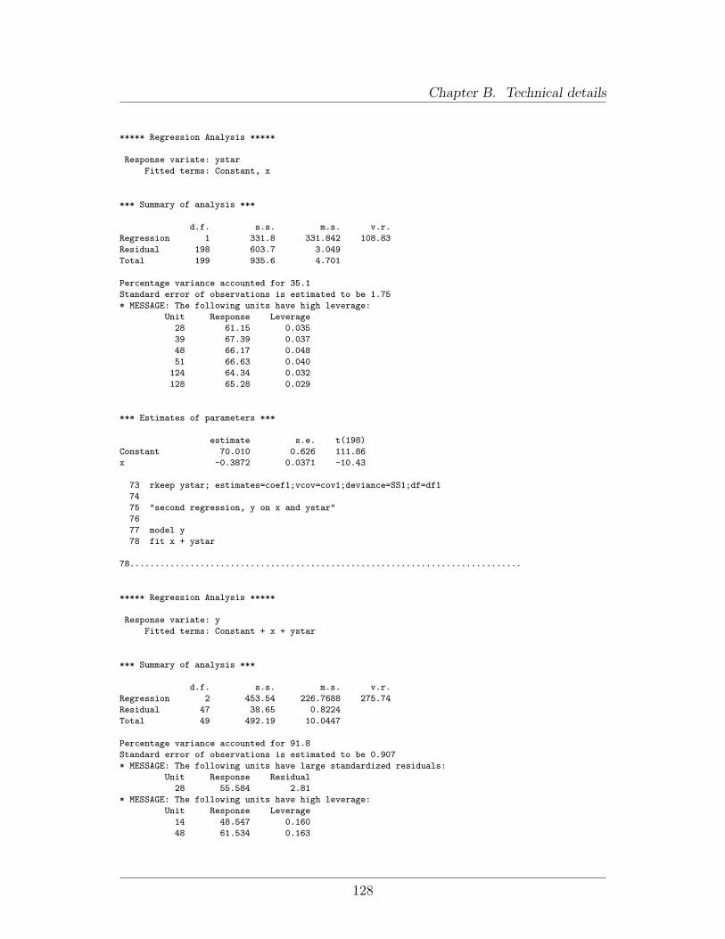
Chapter B. Technical details
***** Regression Analysis *****
Response variate: ystar
Fitted terms: Constant, x
*** Summary of analysis ***
d.f. s.s. m.s. v.r.
Regression 1 331.8 331.842 108.83
Residual 198 603.7 3.049
Total 199 935.6 4.701
Percentage variance accounted for 35.1
Standard error of observations is estimated to be 1.75
* MESSAGE: The following units have high leverage:
Unit Response Leverage
28 61.15 0.035
39 67.39 0.037
48 66.17 0.048
51 66.63 0.040
124 64.34 0.032
128 65.28 0.029
*** Estimates of parameters ***
estimate s.e. t(198)
Constant 70.010 0.626 111.86
x -0.3872 0.0371 -10.43
73 rkeep ystar; estimates=coef1;vcov=cov1;deviance=SS1;df=df1
74
75 "second regression, y on x and ystar"
76
77 model y
78 fit x + ystar
78..............................................................................
***** Regression Analysis *****
Response variate: y
Fitted terms: Constant + x + ystar
*** Summary of analysis ***
d.f. s.s. m.s. v.r.
Regression 2 453.54 226.7688 275.74
Residual 47 38.65 0.8224
Total 49 492.19 10.0447
Percentage variance accounted for 91.8
Standard error of observations is estimated to be 0.907
* MESSAGE: The following units have large standardized residuals:
Unit Response Residual
28 55.584 2.81
* MESSAGE: The following units have high leverage:
Unit Response Leverage
14 48.547 0.160
48 61.534 0.163
128
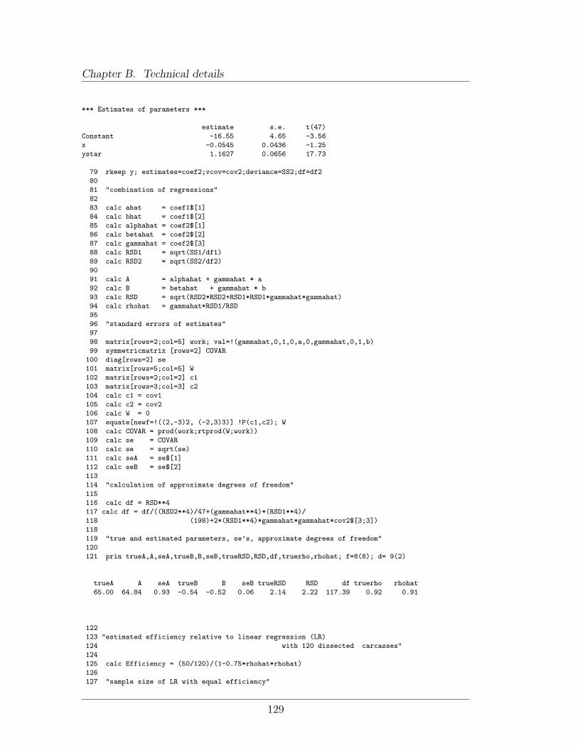
Chapter B. Technical details
*** Estimates of parameters ***
estimate s.e. t(47)
Constant -16.55 4.65 -3.56
x -0.0545 0.0436 -1.25
ystar 1.1627 0.0656 17.73
79 rkeep y; estimates=coef2;vcov=cov2;deviance=SS2;df=df2
80
81 "combination of regressions"
82
83 calc ahat = coef1$[1]
84 calc bhat = coef1$[2]
85 calc alphahat = coef2$[1]
86 calc betahat = coef2$[2]
87 calc gammahat = coef2$[3]
88 calc RSD1 = sqrt(SS1/df1)
89 calc RSD2 = sqrt(SS2/df2)
90
91 calc A = alphahat + gammahat * a
92 calc B = betahat + gammahat * b
93 calc RSD = sqrt(RSD2*RSD2+RSD1*RSD1*gammahat*gammahat)
94 calc rhohat = gammahat*RSD1/RSD
95
96 "standard errors of estimates"
97
98 matrix[rows=2;col=5] work; val=!(gammahat,0,1,0,a,0,gammahat,0,1,b)
99 symmetricmatrix [rows=2] COVAR
100 diag[rows=2] se
101 matrix[rows=5;col=5] W
102 matrix[rows=2;col=2] c1
103 matrix[rows=3;col=3] c2
104 calc c1 = cov1
105 calc c2 = cov2
106 calc W = 0
107 equate[newf=!((2,-3)2, (-2,3)3)] !P(c1,c2); W
108 calc COVAR = prod(work;rtprod(W;work))
109 calc se = COVAR
110 calc se = sqrt(se)
111 calc seA = se$[1]
112 calc seB = se$[2]
113
114 "calculation of approximate degrees of freedom"
115
116 calc df = RSD**4
117 calc df = df/((RSD2**4)/47+(gammahat**4)*(RSD1**4)/
118 (198)+2*(RSD1**4)*gammahat*gammahat*cov2$[3;3])
118
119 "true and estimated parameters, se’s, approximate degrees of freedom"
120
121 prin trueA,A,seA,trueB,B,seB,trueRSD,RSD,df,truerho,rhohat; f=8(8); d= 9(2)
trueA A seA trueB B seB trueRSD RSD df truerho rhohat
65.00 64.84 0.93 -0.54 -0.52 0.06 2.14 2.22 117.39 0.92 0.91
122
123 "estimated efficiency relative to linear regression (LR)
124 with 120 dissected carcasses"
124
125 calc Efficiency = (50/120)/(1-0.75*rhohat*rhohat)
126
127 "sample size of LR with equal efficiency"
129
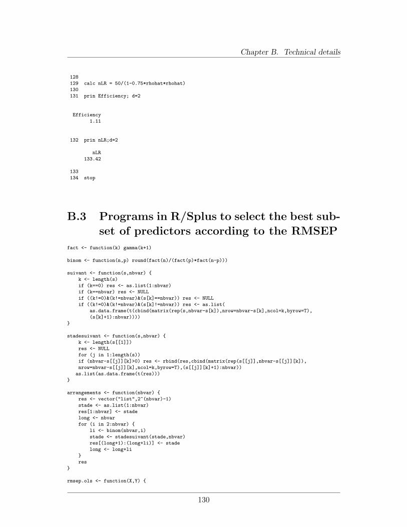
Chapter B. Technical details
128
129 calc nLR = 50/(1-0.75*rhohat*rhohat)
130
131 prin Efficiency; d=2
Efficiency
1.11
132 prin nLR;d=2
nLR
133.42
133
134 stop
B.3 Programs in R/Splus to select the best sub-
set of predictors according to the RMSEP
fact <- function(k) gamma(k+1)
binom <- function(n,p) round(fact(n)/(fact(p)*fact(n-p)))
suivant <- function(s,nbvar) {
k <- length(s)
if (k==0) res <- as.list(1:nbvar)
if (k==nbvar) res <- NULL
if ((k!=0)&(k!=nbvar)&(s[k]==nbvar)) res <- NULL
if ((k!=0)&(k!=nbvar)&(s[k]!=nbvar)) res <- as.list(
as.data.frame(t(cbind(matrix(rep(s,nbvar-s[k]),nrow=nbvar-s[k],ncol=k,byrow=T),
(s[k]+1):nbvar))))
}
stadesuivant <- function(s,nbvar) {
k <- length(s[[1]])
res <- NULL
for (j in 1:length(s))
if (nbvar-s[[j]][k]>0) res <- rbind(res,cbind(matrix(rep(s[[j]],nbvar-s[[j]][k]),
nrow=nbvar-s[[j]][k],ncol=k,byrow=T),(s[[j]][k]+1):nbvar))
as.list(as.data.frame(t(res)))
}
arrangements <- function(nbvar) {
res <- vector("list",2^(nbvar)-1)
stade <- as.list(1:nbvar)
res[1:nbvar] <- stade
long <- nbvar
for (i in 2:nbvar) {
li <- binom(nbvar,i)
stade <- stadesuivant(stade,nbvar)
res[(long+1):(long+li)] <- stade
long <- long+li
}
res
}
rmsep.ols <- function(X,Y) {
130
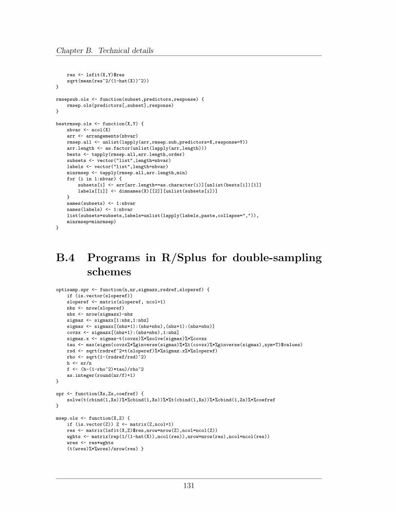
Chapter B. Technical details
res <- lsfit(X,Y)$res
sqrt(mean(res^2/(1-hat(X))^2))
}
rmsepsub.ols <- function(subset,predictors,response) {
rmsep.ols(predictors[,subset],response)
}
bestrmsep.ols <- function(X,Y) {
nbvar <- ncol(X)
arr <- arrangements(nbvar)
rmsep.all <- unlist(lapply(arr,rmsep.sub,predictors=X,response=Y))
arr.length <- as.factor(unlist(lapply(arr,length)))
bests <- tapply(rmsep.all,arr.length,order)
subsets <- vector("list",length=nbvar)
labels <- vector("list",length=nbvar)
minrmsep <- tapply(rmsep.all,arr.length,min)
for (i in 1:nbvar) {
subsets[i] <- arr[arr.length==as.character(i)][unlist(bests[i])[1]]
labels[[i]] <- dimnames(X)[[2]][unlist(subsets[i])]
}
names(subsets) <- 1:nbvar
names(labels) <- 1:nbvar
list(subsets=subsets,labels=unlist(lapply(labels,paste,collapse=",")),
minrmsep=minrmsep)
}
B.4 Programs in R/Splus for double-sampling
schemes
optisamp.spr <- function(n,nr,sigmazx,rsdref,sloperef) {
if (is.vector(sloperef))
sloperef <- matrix(sloperef, ncol=1)
nbz <- nrow(sloperef)
nbx <- nrow(sigmazx)-nbz
sigmaz <- sigmazx[1:nbz,1:nbz]
sigmax <- sigmazx[(nbz+1):(nbz+nbx),(nbz+1):(nbz+nbx)]
covzx <- sigmazx[(nbz+1):(nbz+nbx),1:nbz]
sigmaz.x <- sigmaz-t(covzx)%*%solve(sigmax)%*%covzx
tau <- max(eigen(covzx%*%ginverse(sigmaz)%*%t(covzx)%*%ginverse(sigmax),sym=T)$values)
rsd <- sqrt(rsdref^2+t(sloperef)%*%sigmaz.x%*%sloperef)
rho <- sqrt(1-(rsdref/rsd)^2)
h <- nr/n
f <- (h-(1-rho^2)*tau)/rho^2
as.integer(round(nr/f)+1)
}
spr <- function(Xs,Zs,coefref) {
solve(t(cbind(1,Xs))%*%cbind(1,Xs))%*%t(cbind(1,Xs))%*%cbind(1,Zs)%*%coefref
}
msep.ols <- function(X,Z) {
if (is.vector(Z)) Z <- matrix(Z,ncol=1)
res <- matrix(lsfit(X,Z)$res,nrow=nrow(Z),ncol=ncol(Z))
wghts <- matrix(rep(1/(1-hat(X)),ncol(res)),nrow=nrow(res),ncol=ncol(res))
wres <- res*wghts
(t(wres)%*%wres)/nrow(res) }
131
Chapter B. Technical details
B.5 Logistic regression for dealing with sub-po-
pulationsBy Bas Engel
We will consider an example with two sub-populations, where sampling scheme III consists of one separatesub-sample for each sub-population that is considered. Generalization to several sub-samples is straightforward.
In 1990, throughout the EC, a dissection trial was carried out as a first step towards harmonisation ofmethods for pig classification in the EC. The proposal for the trial (EC, 1989a) specifically mentioned a possibleinterest in differences between sub populations. In The Netherlands at that time there was an interest indifferences between gilts and castrated males. Separate samples were taken for the two sexes in accordance withthe sampling proposal for this EC-trial, thus ensuring sufficient accuracy for a comparison between these twosub-populations. The instrumental carcass measurements were a fat and muscle depth measured by the Henessygrading probe (HGP) (Walstra, 1986).
Separate formulas for gilts and castrated males were calculated and found to be significantly (P ¡ 0.05),although not markedly, different. Due to practical limitations, it was not possible to use separate predictionformulas for the sexes in slaughterhouses in The Netherlands. Therefore, the different formulae for the sexeshad to be combined into one overall formula. Since castrates are generally fatter than gilts, obviously the overallformula should be closer to the formula for gilts for small fat measurements, while for large fat measurementsit should be closer to the formula for castrates. Consequently, in combining the two formulas, the sexes shouldget different weights that depend on the carcass measurements.
To evaluate expressions for these weights, extra information was needed about the proportions of gilts andcastrated males in the pig population, in relation to the prediction variables as collected with the HGP. To thatend an additional large sample of 134158 carcasses was collected from data registered in Dutch slaughterhouses.For all these carcasses gender and HGP measurements were available. No additional dissections were needed.
As was observed before, ignoring the sexes in the regression calculations would not be a statistically soundapproach. Due to the sampling scheme, in the total sample, which is a combination of the sub samples for thetwo sub-populations, gilts are over-represented for the fat carcasses, while castrates are over-represented for thelean carcasses.
Suppose that for a particular pair of observed values for backfat and muscle thickness there are K carcassesin the underlying population with these same carcass measurements. Suppose that k of these carcasses corre-spond to gilts and (K − k) carcasses to castrates. Let p = k/K and 1 − p = (K − k)/K be the correspondingproportions of gilts and castrates in the population. The overall mean lean meat proportion m of the K carcassesin the population would be the best prediction for the carcass on the basis of the HGP values observed. Whenmg and mc are the means corresponding to the k gilts and (K − k) castrates respectively:
m = pmg + (1 − p)mc
The predictions from the separate formulas for gilts and castrates, say yg and yc, are estimates for the meansmg and mc and a natural choice for the overall prediction y is:
y = pyg + (1 − p)yc
The proportions p and (1 − p) depend on the observed fat and muscle depth. For small fat measurements, pwill approach 1 and (1− p) will approach 0 and the prediction y will be close to the prediction yg for a gilt. Forlarge fat measurements, p will approach 0 and (1 − p) will approach 1, and the prediction will be close to theprediction yc for a castrate.
So, the weights employed to combine the separate predictions for the sexes are not constant! They areestimates for the proportions of gilts and castrates in the population, and depend on the observes instrumentalmeasurements. In Engel and Walstra (1993) it is shown how expressions for these weights can be obtained fromthe additional sample where both sex and objective carcass measurements are known. In Engel et al. (2003b)the performance of the Engel & Walstra approach is compared with the use of LR ignoring the sexes. TheEngel & Walstra approach is clearly superior, but the gain depends on the size of the differences between thepopulations.
For the evaluation of a suitable substitute for the RMSE we refer to the calculations in Engel and Walstra(1993) for the 1990 EC-harmonisation trial. There are additional details about the model and the constructionof the overall prediction formula in Engel et al. (2003b).
In Engel et al. (2003b) the potential improvement of the use of separate prediction formulae for sub-populations is investigated in a simulation study. This simulation study is based on practical data from TheNetherlands and Spain. The study shows that a marked bias may occur between sub populations. This biascan be eliminated, and prediction accuracy can be substantially increased, when separate formulae per subpopulation are used. It is likely that such improvements will have a commercial interest for producers thatspecialize in certain sub populations. When the technology for implants improves in the near future, subpopulations will be recognizable automatically in the slaughter-line and the use of different prediction formulaewill become practically feasible. Additional details are provided in Engel et al. (2003b).
132