Statistical Applications in Genetics and Molecular...

Volume 11, Issue 2 2012 Article 5

Statistical Applications in Geneticsand Molecular Biology

COMPUTATIONAL STATISTICAL METHODS FOR GENOMICS ANDSYSTEMS BIOLOGY

Bayesian Sparsity-Path-Analysis of GeneticAssociation Signal using Generalized t Priors

Anthony Lee, University of OxfordFrancois Caron, INRIA Bordeaux

Arnaud Doucet, University of OxfordChris Holmes, University of Oxford

Recommended Citation:Lee, Anthony; Caron, Francois; Doucet, Arnaud; and Holmes, Chris (2012) "Bayesian Sparsity-Path-Analysis of Genetic Association Signal using Generalized t Priors," Statistical Applicationsin Genetics and Molecular Biology: Vol. 11: Iss. 2, Article 5.DOI: 10.2202/1544-6115.1712Available at: http://www.bepress.com/sagmb/vol11/iss2/art5

©2012 De Gruyter. All rights reserved.

Bayesian Sparsity-Path-Analysis of GeneticAssociation Signal using Generalized t Priors

Anthony Lee, Francois Caron, Arnaud Doucet, and Chris Holmes

AbstractWe explore the use of generalized t priors on regression coefficients to help understand the

nature of association signal within “hit regions” of genome-wide association studies. The particulargeneralized t distribution we adopt is a Student distribution on the absolute value of its argument.For low degrees of freedom, we show that the generalized t exhibits “sparsity-prior” properties withsome attractive features over other common forms of sparse priors and includes the well knowndouble-exponential distribution as the degrees of freedom tends to infinity. We pay particularattention to graphical representations of posterior statistics obtained from sparsity-path-analysis(SPA) where we sweep over the setting of the scale (shrinkage/precision) parameter in the priorto explore the space of posterior models obtained over a range of complexities, from very sparsemodels with all coefficient distributions heavily concentrated around zero, to models with diffusepriors and coefficients distributed around their maximum likelihood estimates. The SPA plotsare akin to LASSO plots of maximum a posteriori (MAP) estimates but they characterise thecomplete marginal posterior distributions of the coefficients plotted as a function of the precisionof the prior. Generating posterior distributions over a range of prior precisions is computationallychallenging but naturally amenable to sequential Monte Carlo (SMC) algorithms indexed on thescale parameter. We show how SMC simulation on graphic-processing-units (GPUs) provides veryefficient inference for SPA. We also present a scale-mixture representation of the generalized t priorthat leads to an expectation-maximization (EM) algorithm to obtain MAP estimates should onlythese be required.

KEYWORDS: sparsity prior, Bayesian analysis, genome-wide association studies

Author Notes: Anthony Lee, Oxford-Man Institute and Department of Statistics, University ofOxford, UK. François Caron, INRIA Bordeaux Sud-Ouest and Institut de Mathématiques deBordeaux, University of Bordeaux, France. Arnaud Doucet, Institute of Statistical Mathematics,Japan and Department of Statistics, University of Oxford, UK. Chris Holmes, Department ofStatistics and Oxford-Man Institute and Wellcome Trust Centre for Human Genetics, Universityof Oxford, and MRC Harwell, UK. Anthony Lee would like to acknowledge the support of theUniversity of Oxford Clarendon Fund Scholarship and the Oxford-Man Institute. Chris Holmeswould like to acknowledge support for this research by the Medical Research Council, Oxford-ManInstitute and Wellcome Trust Centre for Human Genetics, Oxford. The authors would additionallylike to thank the organizers of the recent meeting on "Computational statistical methods forgenomics and system biology" held at the Centre de Recherches Mathématiques, Montreal.

1 IntroductionGenome-wide association studies (GWAS) have presented a number of interest-ing challenges to statisticians (Balding, 2006). Conventionally GWAS use singlemarker univariate tests of association, testing marker by marker in order to highlight“hit regions” of the genome showing evidence of association signal. The motiva-tion for our work concerns methods in Bayesian sparse multiple regression analysisto characterise and decompose the association signal within such regions spanningpossibly hundreds of markers. Hit-regions typically cover loci in high linkage dis-equilibrium (LD) which leads to strong correlation between the markers and makesmultiple regression analysis non-trivial. A priori we would expect only a smallnumber of markers to be responsible for the association and hence priors that in-duce sparsity are an important tool to aid understanding of the genotype-phenotypedependence structure; an interesting question being whether the association signalis consistent with a single causal marker or due to multiple effects. We restrict at-tention to case-control GWAS, i.e. binary phenotypes, these being by far the mostprevalent although generalisations to other exponential family likelihoods or non-linear models is relatively straightforward.

In the non-Bayesian literature sparse regression analysis via penalised like-lihood has gained increasing popularity since the seminal paper on the LASSO(Tibshirani, 1996, 2011). The LASSO estimates have a Bayesian interpretation asmaximum a posteriori (MAP) statistics under a double exponential prior on regres-sion coefficients p(β )∝ exp(−λ ∑ j |β j|) and it is known that, unlike ridge penaltiesusing a normal prior, the Lasso prior tends to produce ‘sparse’ solutions in that asan increasing function of the regularisation penalty λ more and more of the MAPestimates will be zero. From a Bayesian perspective the use of MAP estimates holdslittle justification, see the discussion of Tibshirani (2011), and in Park and Casella(2008) they explore full Bayesian posterior analysis with Lasso double-exponentialpriors using Markov chain Monte Carlo (MCMC) to make inference. While theLasso penalty / prior is popular there is increasing awareness that the use of iden-tical ‘penalization’ on each coefficient, e.g. λ ∑

pj=1 |β j|, can lead to unacceptable

bias in the resulting estimates (Fan and Li, 2001). In particular, coefficients getshrunk towards zero even when there is overwhelming evidence in the likelihoodthat they are non-zero. This has motivated use of sparsity-inducing non-convexpenalties which reduce bias in the estimates of large coefficients at the cost of in-creased difficulty in computing. Of note we would mention the “adaptive” methods(Zou, 2006, Zou and Li, 2008) in the statistics literature and iteratively reweightedmethods (Candes, Wakin, and Boyd, 2008, Chartrand and Yin, 2008) in the signalprocessing literature; although these papers are only concerned with MAP estima-

1

Lee et al.: Sparsity-Path-Analysis with Generalized t Priors

Published by De Gruyter, 2012

analysis.In the context of GWAS there have been recent illustrations of the use of

adaptive sparsity priors and MAP estimation (Hoggart, Whittaker, De Iorio, andBalding, 2008), reviewed and compared in Ayers and Cordell (2010). In Hoggartet al. (2008) they use the Normal-Exponential-Gamma sparsity-prior of Griffin andBrown (2007) to obtain sparse MAP estimates from logistic regression. The use ofcontinuous sparse priors can be contrasted with an alternative approach using twocomponent mixture priors such as in George and McCulloch (1993) which adopt adistribution containing a spike at zero and another component with broad scale. Co-efficients are then a posteriori classified into either state, relating to whether theircorresponding variables (genotypes) are deemed predictively irrelevant or relevant.In the GWAS setting the two-component mixture prior has been explored by Wil-son, Iversen, Clyde, Schmidler, and Schildkraut (2010) and Fridley (2009). Formodel exploration the sparsity prior has some benefits in allowing the statisticiansto visualize the regression analysis over a range of scales / model complexities.

In this paper we advocate the use of the generalized t prior, first consideredin McDonald and Newey (1988), on the regression coefficients and a full Bayesiananalysis. The generalized t prior we adopt is a Student distribution on the absolutevalue of the coefficient. We demonstrate it has a number of attractive features as a‘sparsity prior’ in particular due to its simple analytic form and interpretable param-eters. In applications the setting of the scale parameter in the prior is the key taskthat affects the sparsity of the posterior solution. We believe much is to be gained inexploring the continuum of posterior models formed by sweeping through the scaleof the prior, even over regions of low posterior probability, in an exploratory ap-proach we term sparsity-path-analysis (SPA). This leads towards providing graph-ical representations of the posterior densities that arise as we move from the mostsparse models with all coefficient densities heavily concentrated around the originthrough to models with diffuse priors and coefficients distributed around their max-imum likelihood estimates. We stress that even though parts of this model spacehave low probability, they have utility and are interesting in gaining a fuller un-derstanding of the predictor-response (genotype-phenotype) dependence structure.SPA is an exploratory tool that is computationally challenging but highly suitedto sequential Monte Carlo (SMC) algorithms indexed on the scale parameter andsimulated in parallel on graphics cards using graphical processing units (GPUs).

The generalized t as a prior for Bayesian regression coefficients was firstsuggested by McDonald and Newey (1988) and more recently in the context ofsparse MAP estimation for normal (Gaussian) likelihoods (Lee, Caron, Doucet,and Holmes, 2010a, Cevher, 2009, Armagan, Dunson, and Lee, 2011), and usingMCMC for a full Bayesian linear regression analysis in Armagan et al. (2011).

tion, there being no published articles to date detailing the use of full Bayesian

2

Statistical Applications in Genetics and Molecular Biology, Vol. 11 [2012], Iss. 2, Art. 5

http://www.bepress.com/sagmb/vol11/iss2/art5DOI: 10.2202/1544-6115.1712

double-pareto distribution but we prefer to use the terminology of the generalizedt as we feel it is more explicit and easier to interpret as such. Our contribution inthis paper is to consider a full Bayesian analysis of logistic regression models withgeneralized t priors in the context of GWAS applications for which we developSMC samplers and GPU implementation. The GPU implementation is important inpractice; in the GWAS analysis it reduces run-time from over five days to hours. Wepay particular attention to developing graphical displays of summary statistics fromthe joint posterior distribution over a wide range of prior precisions; arguing thatparts of the model space with low probability have high utility and are informativeto the exploratory understanding of regression signal.

In Section 2 we introduce the generalized t prior and show that it has a scale-mixture representation and exhibits sparsity type properties for regression analysis.Section 3 provides a brief description of the genetic association data and simulatedphenotypes used in our methods development. Section 4 concerns computing pos-terior distributions over a range of prior scale parameters using sequential MonteCarlo algorithms simulated on GPUs. Section 5 deals with graphical display ofSPA statistics and plots of posterior summary statistics over the path of scales. Weconclude with a discussion in Section 6.

2 Generalized t prior for sparse regression analysisIn Bayesian logistic regression analysis we are given a data set {X,y}, of an (n×p) predictor matrix X and an (n× 1) vector of binary phenotypes (or responsevariables) y. We adopt a prior p(βββ ) on the p regression coefficients from which thelog-posterior updates as,

log p(βββ |X,y,a,c) = log f (y|X,βββ )+ log p(βββ )+C

where f (·) is the likelihood function, C is a constant independent of βββ , and

f (y|X,βββ ) =n

∏i=1

(pi)yi(1− pi)

1−yi

pi = logit−1(xiβββ ).

In this paper we propose the generalized t distribution as an interesting priorfor each component of βββ , which has the form of a Student density on the Lq-normof its argument, (McDonald and Newey, 1988),

p(β j|µ,a,c,q) =q

2ca1/qB(1/q,a)

(1+|β j−µ|q

acq

)−(a+1/q)

(1)

In Cevher (2009), Armagan et al. (2011) the prior is referred to as a generalized

3



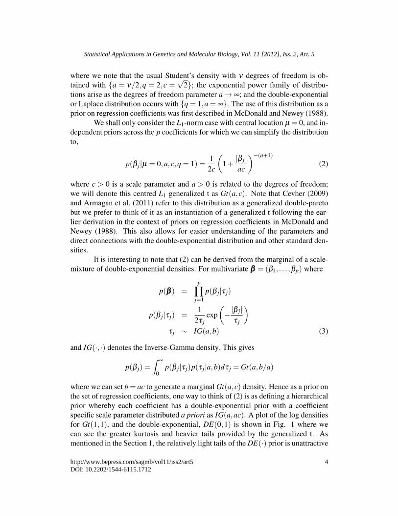
where we note that the usual Student’s density with ν degrees of freedom is ob-tained with {a = ν/2,q = 2,c =

√2}; the exponential power family of distribu-

tions arise as the degrees of freedom parameter a→ ∞; and the double-exponentialor Laplace distribution occurs with {q = 1,a = ∞}. The use of this distribution as aprior on regression coefficients was first described in McDonald and Newey (1988).

We shall only consider the L1-norm case with central location µ = 0, and in-dependent priors across the p coefficients for which we can simplify the distributionto,

p(β j|µ = 0,a,c,q = 1) =12c

(1+|β j|ac

)−(a+1)

(2)

where c > 0 is a scale parameter and a > 0 is related to the degrees of freedom;we will denote this centred L1 generalized t as Gt(a,c). Note that Cevher (2009)and Armagan et al. (2011) refer to this distribution as a generalized double-paretobut we prefer to think of it as an instantiation of a generalized t following the ear-lier derivation in the context of priors on regression coefficients in McDonald andNewey (1988). This also allows for easier understanding of the parameters anddirect connections with the double-exponential distribution and other standard den-sities.

It is interesting to note that (2) can be derived from the marginal of a scale-mixture of double-exponential densities. For multivariate βββ = (β1, . . . ,βp) where

p(βββ ) =p

∏j=1

p(β j|τ j)

p(β j|τ j) =1

2τ jexp(−|β j|τ j

)τ j ∼ IG(a,b) (3)

and IG(·, ·) denotes the Inverse-Gamma density. This gives

p(β j) =∫

∞

0p(β j|τ j)p(τ j|a,b)dτ j = Gt(a,b/a)

where we can set b = ac to generate a marginal Gt(a,c) density. Hence as a prior onthe set of regression coefficients, one way to think of (2) is as defining a hierarchicalprior whereby each coefficient has a double-exponential prior with a coefficientspecific scale parameter distributed a priori as IG(a,ac). A plot of the log densitiesfor Gt(1,1), and the double-exponential, DE(0,1) is shown in Fig. 1 where wecan see the greater kurtosis and heavier tails provided by the generalized t. Asmentioned in the Section 1, the relatively light tails of the DE(·) prior is unattractive

4



Figure 1: Plot of log density under the Gt(1,1) (solid line) and the Lasso priorDE(0,1) (dashed line).

as it tends to shrink large values of the coefficients even when there is clear evidencein the likelihood that they are predictively important.

We are interested with inferring and graphing the regression coefficients’posterior distributions over a range of values for c for fixed a, an exploratory pro-cedure we call sparsity-path-analysis. But first it is instructive to examine the formof the MAP estimates obtained under the generalized t prior as this sheds light ontheir utility as sparsity priors.

2.1 MAP estimates via the EM algorithm

The optimization problem associated with obtaining the MAP estimates for βββ underthe generalized t-distribution prior is not concave. However, one can find localmodes of the posterior by making use of the scale-mixture representation (3) andusing the EM algorithm with the hierarchical scale parameters τττ = τ1:p as latentvariables. Indeed, each iteration of EM takes the form

βββ(t+1) = argmax

βββ

log f (y|X,βββ )+∫

log[p(βββ |τττ)]p(τττ|βββ (t),a,b)dτττ

where b = ac. The conjugacy of the inverse-gamma distribution with respect to theLaplace distribution gives

τ j|β (t)j ,a,b∼ IG(a+1,b+ |β (t)

j |)

5



allowing for different prior parameters for each coefficient, and with p(βββ |τττ) =∏

pj=1 p(β j|τ j) = ∏

pj=1 1/(2τ j)exp(−|β j|/τ j) yields


βββ

log f (y|X,βββ )−p

∑j=1|β j|

∫ 1τ j

p(τ j|β (t)j ,a,b)dτ j

where the expectation of 1/τ j given τ j ∼ IG(a+1,b+ |β (t)j |) is (a+1)/(b+ |β (t)

j |).As such, one can find a local mode of the posterior p(βββ |y,X,a,b) by starting atsome point βββ

(0) and then iteratively solving


βββ

log f (y|X,βββ )−p

∑j=1

w(t)j |β j| (4)

where

w(t)j =

a+1

b+ |β (t)j |

=a+1

ac+ |β (t)j |

For logistic regression the update (4) is a convex optimization problem for whichstandard techniques exist. We can see the connection to the Lasso as with a→ ∞

we find w(t)j →

1c , where λ = 1/c is the usual Lasso penalty.

2.2 Oracle properties of the MAP

In the penalized optimization literature, some estimators are justified at least par-tially by their possession of the oracle property: that for appropriate parameterchoices, the method performs just as well as an oracle procedure in terms of select-ing the correct predictors and estimating the nonzero coefficients correctly asymp-totically in n when the likelihood is Gaussian. Other related properties includeasymptotic unbiasedness, sparsity and continuity in the data (Fan and Li, 2001).Penalization schemes with the oracle property include the smoothly clipped abso-lute deviation method (Fan and Li, 2001), the adaptive lasso (Zou, 2006) and theone-step local linear approximation method (Zou and Li, 2008).

For the generalized t-distribution, the MAP estimate obtained using thisprior has been examined in (Lee et al., 2010a, Cevher, 2009, Armagan et al., 2011),all of which derive the expectation-maximisation algorithm for finding a local mode

6



of the posterior. It is straightforward to establish that the estimate is asymptot-ically unbiased, sparse when c < 2

√(a+1)/a and continuous in the data when

c =√

(a+1)/a following the conditions laid out in Fan and Li (2001). Armaganet al. (2011) shows that this scheme satisfies the oracle property if simultaneouslya→ ∞, a/

√n→ 0 and ac

√n→C < ∞ for some constant C.

It is worth remarking that the oracle property requires the prior on βββ todepend on the number of observations n. This is in conflict with conventionalBayesian analysis, where priors represent beliefs about the data generating mecha-nism irrespective of the number of observations that will be obtained. In addition,for a given application it may not be the case that n and p are in the realm of asymp-totic relevance for this property to be meaningful.

2.3 Comparison to other priors

There have been a number of sparsity prior representations advocated recently inthe literature, although it is important to note that most of the papers deal solelywith MAP estimation and not full Bayesian analysis. To name a few importantcontributions we highlight the normal-gamma, normal-exponential-gamma (NEG)and the Horseshoe priors, see (Griffin and Brown, 2010, Caron and Doucet, 2008,Griffin and Brown, 2007, Carvalho, Polson, and Scott, 2010). Like all these priorsthe Gt(·, ·) shares the properties of sparsity and adaptive shrinkage, allowing forless shrinkage on large coefficients as shown in Fig. 2 for a normal observation,and a scale-mixture representation which facilitates an efficient EM algorithm toobtain MAP estimates.

In Table 1 we have listed the log densities for the sparsity-priors mentionedabove. From Table 1 we see an immediate benefit of the generalized t density isthat it has a simple analytic form compared with other sparsity-priors and is wellknown and understood by statisticians, which in turn aids explanation to data own-ers. The generalized t is also easy to compute relative to the NEG, normal-gammaand Horseshoe priors which all involve non-standard computation, making themmore challenging to implement and less amenable to fast parallel GPU simulation.Finally, the setting of the parameters of the generalized t is helped as statisticiansare used to thinking about degrees of freedom and scale parameters of Student’sdensities. We believe this will have an impact on the attractiveness of the prior tonon-expert users outside of sparsity researchers.

7



Figure 2: Estimate of the posterior mean under a single normal observation, y, forthe Gt(a= 1,c= 0.1) (blue dashed) and Gt(a= 4,c= 0.1) (red dashed). We can seethe sparsity by the setting to zero around y = 0 and the approximate unbiasednesswith reduction in shrinkage as |y|>> 0.

log p(β j)

double-exponential −λ |β j|+C

normal-gamma (12 −λ ) log |β j|− logKλ−1/2

(|β j|λ

)+C

NEG − β 2

4λ 2 − logD−2(λ+ 12 )

(|β |λ

)+C

Horseshoe log[∫

∞

0 (2τ2λ 2)−1/2 exp(− β 2

j2τ2λ 2

)(1+λ )−2dλ

]+C

Gt(a,c) −(a+1) log(

1+ |β j|ac

)+C

Table 1: Log densities for the double-exponential and various sparsity-priors, upto an additive prior-specific constant C. K(·) denotes a Bessel function of the thirdkind and Dv(z) is the parabolic cylinder function. The Horseshoe prior does nothave an analytic form.

8



3 Genotype DataIn the development and testing of the methods in this paper we made use of anony-mous genotype data obtained from the Wellcome Trust Centre for Human Genetics(WTCHG), Oxford. The data consists of a subset of single-nucleotide polymor-phisms (SNPs) from a genome-wide data set originally gathered in a case-controlstudy to identify colorectal cancer risk alleles. The data set we consider consists ofgenotype data for 1859 subjects on 184 closely spaced SNPs from a hit-region onchromosome 18q. We standardise the columns of X to be mean zero and unit stan-dard deviation. A plot of the correlation structure across the first 100 markers in theregion is shown in Fig. 3. We can see the markers are in high LD with block likestrong correlation structure that makes multiple regression analysis challenging.

Figure 3: Plot of correlation structure across the first 100 adjacent genotype markersfrom chromosome 18q.

We generated pseudo-phenotype data, y, by selecting at random five lociand generating coefficients, β ∼ N(0,0.22), judged to be realistic signal sizes seenin GWAS (Stephens and Balding, 2009). All other coefficients were set to zero.We then generated phenotype, case-control, binary y data by sampling Bernoullitrials with probability given by the logit of the log-odds, xiβββ , for an individual’sgenotype xi. We considered two scenarios. The first when we construct a genotypematrix of 500 individuals using the five relevant markers and an additional 45 “null”markers whose corresponding coefficients were zero, i.e. a subset of the data from

9



the study. The second data set uses all available markers and all subjects to createa (1859× 184) design matrix. To clarify, all covariate data used in the followingexamples is real genotype data from chromosome 18q on individuals genotypedas part of the WTCHG study. However the phenotype (response variable) y issimulated due to confidentiality issues.

4 Sequential Monte Carlo and graphic card simula-tion

We propose to explore the posterior distributions of βββ |X,y,a,c with varying c =b/a via Sequential Monte Carlo (SMC) sampler methodology (Del Moral, Doucet,and Jasra, 2006). In particular, we let the target distribution at time t be πt(βββ ) =p(βββ |X,y,a,bt/a) with t = {1, . . . ,T} and some specified sequence {bt}T

t=1 wherebi > bi+1 and bT is small enough for the prior to dominate the likelihood with allcoefficients posterior distributions heavily concentrated around zero, and b1 largeenough for the prior to be diffuse and have limited impact on the likelihood. Inorder to compute posterior distributions over the range of {bt}T

t=1 we make use ofsequential Monte Carlo samplers indexed on this sequence of scales.

It is important to note that we cannot evaluate

πt(βββ ) =p(y|X,βββ )p(βββ |a,bt)∫

p(y|X,βββ )p(βββ |a,bt)dβββ

since we cannot evaluate the integral in the denominator, the marginal likelihood ofy. However, we can evaluate γt(βββ ) = Ztπt(βββ ) where Zt =

∫p(y|X,βββ )p(βββ |a,bt)dβββ .

At time t we have a collection of N particles {βββ (i)t }N

i=1 and accompanyingweights {W (i)

t }Ni=1 such that the empirical distribution

πNt (dβββ ) =

N

∑i=1

W (i)t δ

βββ(i)t(dβββ )

is an approximation of πt . The weights are given by

W (i)t =

W (i)t−1wt(βββ

(i)t−1,βββ

(i)t )

∑Nj=1W ( j)

t−1wt(βββ( j)t−1,βββ

( j)t )

(5)

where

wt(βββ(i)t−1,βββ

(i)t ) =

γt(βββ(i)t )Lt−1(βββ

(i)t ,βββ

(i)t−1)

γt−1(βββ(i)t−1)Kt(βββ

(i)t−1,βββ

(i)t )

(6)

10



We use an Markov chain Monte Carlo (MCMC) kernel Kt with invariant distributionπt to sample each particle βββ

(i)t , i.e. βββ

(i)t ∼ Kt(βββ

(i)t−1, ·). The backwards kernel Lt−1

used to weight the particles is essentially arbitrary but we use the reversal of Kt

Lt−1(βββ t ,βββ t−1) =πt(βββ t−1)Kt(βββ t−1,βββ t)

πt(βββ t)

so that the weights in (6) are given by

wt(βββ(i)t−1,βββ

(i)t ) =

γt(βββ(i)t−1)

γt−1(βββ(i)t−1)

as suggested in (Crooks, 1998, Neal, 2001, Del Moral et al., 2006).Since the weights do not depend on the value of βββ t , it is better to resample

the particles before moving them according to Kt , when resampling is necessary.We resample the particles when the effective sample size (ESS) (Liu and Chen,1995) is below (3/4)N. Also note that even if we knew the normalizing constantsZt−1 and Zt , they would have no impact since the weights are normalized in (5). Wecan however obtain an estimate of Zt/Zt−1 at time t via

Zt

Zt−1=∫

γt(βββ t−1)

γt−1(βββ t−1)πt−1(βββ t−1)dβββ t−1 (7)

≈N

∑i=1

W (i)t−1wt(βββ

(i)t−1,βββ

(i)t ) =

Zt

Zt−1(8)

which allows one to estimate the unnormalized marginal density Zt/Z1 for each

value of bt via ZtZ1

= ∏tt=2

ZtZt−1

.If we additionally give logb a uniform prior on [logbT , logb1], these unnor-

malized marginal densities can also be used to weight the collections of particlesat each time, allowing us to approximate the distribution of βββ with b marginalizedout.

πNt (dβββ ) =

1

∑Tt=1

ZtZ1

T

∑t=1

Zt

Z1

N

∑i=1

W (i)t δ

βββ(i)t(dβββ ) (9)

Note that this is equivalent to systematic sampling of the values of b, and that animproper uniform prior for logb on (−∞,∞) would induce an improper posteriorfor βββ .

11



4.1 Further Details

For analysis of the data with n = 500 and p = 50, we use N = 8192 particles and weconsider two settings of a = 1 and a = 4 with T = 450 and T = 350 respectively,with the lower T for a = 4 explained by the low marginal likelihood associatedwith small values of b when a is large. We set bt = 2(0.98)t−1 for t ∈ {1, . . . ,T}.Given the nature of the posterior, a simple p-dimensional random walk Metropolis-Hastings kernel does not seem to converge quickly. We found that using a cycleof kernels that each update one element of βββ using a random walk proposal withvariance 0.25 mixed better for a given amount of computation than a p-dimensionalrandom walk proposal, which is consistent with Neal and Roberts (2006). To ensurethat our kernels mix fast enough to get good results we construct Kt by cycling thiscycle of kernels 5 times. This is computationally demanding since each step of thealgorithm consists of 5N p MCMC steps, each of which has a complexity in O(n),since the calculation of the likelihood requires us to update Xβββ for a change in oneelement of βββ .

In fact, computation on a 2.67GHz Intel Xeon requires approximately 20hours of computation time with these settings and T = 450. However, we imple-mented the algorithm to run on an NVIDIA 8800 GT graphics card using the Com-pute Unified Device Architecture (CUDA) parallel computing architecture, usingthe SMC sampler framework in Lee, Yau, Giles, Doucet, and Holmes (2010b) totake advantage of the ability to compute the likelihood in parallel for many parti-cles. On this hardware, the time to run the algorithm is approximately 30 minutesfor T = 450, giving around a 40 fold speedup.

The initial particles for t = 1 are obtained by running an MCMC algorithmtargeting π1 for a long time and picking suitably thinned samples to initialize theparticles. The weights of each particle start off equal at 1/N. While not ideal, trivialimportance sampling estimates have a very low ESS for reasonable computationalpower and, in any case, the SMC sampler methodology requires us to have a rapidlymixing MCMC kernel for our resulting estimates to be good.

The particle with the highest posterior density at each time is used as aninitial value for the MAP algorithm described in Section 2.1. The density of theestimated MAP from this initial value is compared with the MAP obtained by us-ing the previous MAP as an initial value and the estimate with the higher posteriordensity is chosen as the estimated MAP. This has the effect of both removing vari-ables that the original algorithm has not removed and keeping variables in that theoriginal algorithm has not, as it is not possible for the MAP algorithm to explorethe multimodal posterior density fully.

While the independence of the weights of the particles makes it possibleto adapt the selection of bt to allow aggressive changes in b while maintaining

12



a given ESS (Del Moral, Doucet, and Jasra, 2011, Bornn, Doucet, and Gottardo,2010), we found that this scheme had a poor effect on the quality of our samples.This is primarily because we discovered that our cycle length for Kt was not largeenough to get the particles to approximate πt after a large change in b, despite asmall change in ESS. Increasing the cycle length has an essentially linear effecton the computational resources required, so this appears to be a poor option forreducing the computational complexity of the method. In addition, having bt on alogarithmic schedule enables us to use the simple approximation to the posterior ofβββ |X,y,a given by (9).

For the larger experiment with n = 1859, p = 184 and a = 4, we use thesame parameters except that we used the schedule bt = (0.98)t−1 with T = 250.This was sufficient to capture a wide range of model complexities. Nevertheless,the running time for this experiment on our GPU was 7.5 hours. This demonstratesthe key practical benefit to using GPUs, as a similar run on a single CPU wouldtake upwards of 5 days.

4.2 Tuning the SMC sampler

Following exploratory analysis we found that bt = b1(0.98)t−1 worked well, andthat setting b1 equal to one or two produced a diffuse enough prior when samplesize was in the 100s or 1000s, as is the situation in GWAS.

In practice, one will have to experiment with the parameters of the SMCsampler in order to ensure satisfactory results. In particular, given an MCMC kernelKt , one must decide how many cycles should be performed per time step to mixadequately in relation to how quickly one wishes to decrease b. In an ideal scenario,Kt produces essentially independent samples from πt regardless of the current setof particles. This would allow one to set {bt}T

t=1 such that computational power isonly spent in areas of b that are of interest. In practice, however, Kt will often onlymix well locally and so small steps in b are desirable to ensure that the Monte Carloerror in the scheme does not dominate the results. It is difficult to characterize therelationship between the number of cycles of Kt to perform and how aggressivelyone can decrease b in general. However, in this context, one might not want todecrease b too quickly anyway, so that a smooth picture of the relationship betweensuccessive posteriors can be visualized.

The number of particles, N, is a crucial parameter that should be set atsuch a level that some fraction of N can provide a suitable approximation of eachintermediate target density. In practice, the number of effective samples is lowerthan N and resampling when the ESS is low is an attempt to ensure that this numberis controlled. It is standard practice to choose to resample particles when the ESS

13



is below CN for some C ≥ 1/2. We choose to resample the particles when the ESSfell below (3/4)N.

A recommended way to test whether the sampler is performing acceptablyis to run an MCMC scheme with fixed b = bt for some intermediate value of tand compare the samples one obtains after convergence with those produced by theSMC sampler. This is possible in this context because the posterior is not particu-larly troublesome to sample from for fixed b with a sensible kernel.

Finally it is worth noting that if the aim was to infer a single distributiongiven a single setting of c = b/a, or with a prior on c, one could achieve betterresults via one long MCMC run. The benefit of the SMC sampler is that it pro-vides a unified method to obtain all of the exploratory statistics and estimates of themarginal likelihood in a single run.

5 Sparsity-Path-AnalysisLasso plots of MAP estimates as functions of the penalty parameter λ are a highlyinformative visual tool for statisticians to gain an understanding of the relative pre-dictive importance of covariates over a range of model complexities (Hastie, Tib-shirani, and Friedman, 2009). However, MAP statistics are single point estimatesthat fail to convey the full extent of information contained within the joint posteriordistribution. One key aim of this report is to develop full Bayesian exploratory toolsthat utilize the joint posterior information.

In this section we describe graphical displays of summary statistics con-tained in SPA results by first considering the n = 500, p = 50 data set describedabove. The indices of the variables with non-zero βββ ’s are I = {10,14,24,31,37}with corresponding βββI = {−0.2538,0.4578,−0.1873,−0.1498,0.0996}. In theGt(a,c) prior we found the Gt(a = 1,c), or Gt(a = 4,c), to be good default set-tings the degrees of freedom parameter, with both leading to heavy tails. We ranthe SMC-GPU sampler described above and then generated a number of plots usingthe set of particles and their weights.

5.1 Path plots

In Fig. 4 we plot four graphs of summary statistics obtained from the SMC sampleracross a range of scales log(c) ∈ (−8,0).

14



(a) MAPs (b) absolute medians

(c) posterior density (d) concentrations

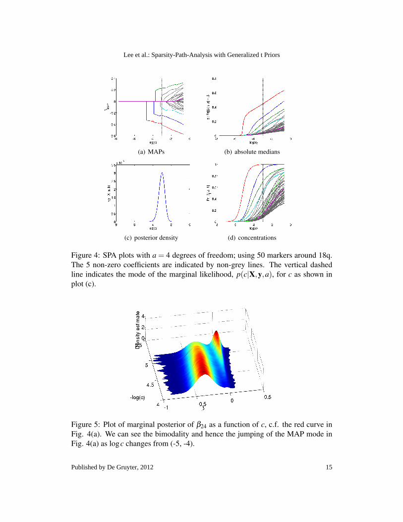
Figure 4: SPA plots with a = 4 degrees of freedom; using 50 markers around 18q.The 5 non-zero coefficients are indicated by non-grey lines. The vertical dashedline indicates the mode of the marginal likelihood, p(c|X,y,a), for c as shown inplot (c).

Figure 5: Plot of marginal posterior of β24 as a function of c, c.f. the red curve inFig. 4(a). We can see the bimodality and hence the jumping of the MAP mode inFig. 4(a) as logc changes from (-5, -4).

15



(a) MAPs (b) absolute medians

(c) posterior density (d) concentrations

Figure 6: SPA plots with a = 1 degrees of freedom; using 50 markers around 18q.This Figure should be compared with Fig. 4 using a = 4 degrees of freedom.

other than gray. One can observe that the MAP paths are non-smooth inlog(c) such that the modes suddenly jump away from zero. This is a propertyof the non-log-concavity of the posterior distributions; such that the marginalposterior densities can be bimodal with one mode at β j = 0 and another awayfrom zero. As c increases the MAP mode at zero decreases and at some pointthe global mode switches to the mode at β j 6= 0. This can be seen clearly inFig. 5 where we plot the marginal posterior distribution of β24 over the rangelogc ∈ (−5,−4); c.f. β24 is shown as the red curve in Fig. 4(a). We can seein Fig. 5 the non-concavity of the posterior density and how the global modejumps from 0 to ≈ −.04 as logc is around −4.75. As mentioned above theMAP is found by iterating the EM algorithm beginning from the particle withlargest posterior density.

(b) Median plots: In Fig. 4(b) we plot the absolute value of the median of themarginal distribution of β j’s. This is a plot of z j(log[c]) vs. logc, for j =1, . . . , p, where,

(a) MAP plots: In Fig. 4(a) we plot the MAP paths of all 50 coefficients movingfrom the most sparse models with c = e−8 where all βββ MAP = 0 through toc = 1 when all βββ MAP 6= 0. The true non-zero coefficients are plotted in colors

16



where F−1β j

(·) is the inverse cumulative posterior distribution of β j,

Fβ j(x|c) =∫ x

−∞

p(β j|X,y,a,c)dβ j

and where p(β j|X,y,a,c) is the marginal posterior distribution of β j givenc; p(β j|X,y,a,c) =

∫ℜp−1 p(β j,β− j|X,y,a,c)dβ− j where {− j} indicates all

indices other than the jth. The plot of absolute medians gives an indicationof how quickly the posterior distributions are moving outward away from theorigin as the precision of the prior decreases. By plotting on the absolutescale we are better able to compare the coefficients with one another and wealso see that, unlike the MAPs, the medians are smooth functions of c.

(c) Posterior for scale c: In Fig. 4(c) we show the marginal posterior distributionp(c|X,y,a),

p(c|X,y,a) =∫

ℜpp(c,βββ |X,y,a)dβββ .

The posterior on c graphs the relative evidence for particular prior scale. Themode of Fig. 4(c),

c = argmaxc

p(c|X,y,a)

is indicated on plots (a),(b),(d) by a vertical dashed line.(d) Concentration plots: In Fig. 4(d) we plot the concentration of the marginal

posteriors of β j’s around the origin, as well as the a priori concentration (lightgreen). In particular, for user specified tolerance ∆, this is a plot of V (c) vs.c where,

V (c) = 1−∫

∆

−∆

p(β j|X,y,a,c)dβ j = 1−Pr(β j ∈ (−∆,∆)|X,y,a,c)

This is a direct measure of the predictive relevance of the corresponding co-variate (genotype). In Fig. 4(d) we have set ∆ = 0.1 although this is a userset parameter that can be specified according to the appropriate level belowwhich a variable is not deemed important.

Taken together the SPA plots highlight the influential genotypes and therelative evidence for their predictive strength. We can also gain an understandingof the support in the data for differing values of log(c). Having generated the SPAplots it is interesting to compare the results of changing the degrees of freedom fromGt(a = 4,c) to Gt(a = 1,c). In Fig. 6 we show plots corresponding to Fig. 4 butusing a = 1. We can see that, as expected, Gt(a = 1,c) produces sparser solutionswith only three non-zero MAP estimates at the mode of the posterior, c. Moreover,

z j(c) = |F−1β j

(0.5|c)|

17



5.2 Individual coefficient plots

(a) a = 4, j = 14 (b) a = 4, j = 24

(c) a = 4, j = 31 (d) a = 4, j = 1

Figure 7: Stats for individual coefficients from Fig. 4 with a = 4. We plot 90%credible intervals (green), median (black), mean (blue) and MAP (red).

Examination of the plots in Fig. 4 may highlight to the statistician someinteresting predictors to explore in greater detail. Individual coefficient plots ofsummary statistics can be produced to provide greater information on the posteriordistributions. In Fig. 7 we show summary plots for four representative coefficientswith their 90% credible intervals (green), median (black), mean (blue) and MAP(red). These are obtained from the set of weighted SMC particles. We can see thatas expected the mean and median are smooth functions of the prior scale, whichthe MAP can exhibit the characteristic jumping for bimodal densities. In Fig. 8 weshow corresponding density estimates. These coefficients were chosen to representmarkers with strong association Fig. 7(a), weaker association Fig. 7(b),(c) and noassociation Fig. 7(d). We can see in the plots for Fig. 7(d) and Fig. 8(d) that fora null marker with no association signal the MAP appears to be much smother inlog(c).

Equivalent plots but for a = 1 are shown in Fig. 9 and Fig. 10 where wesee the greater sparsity induced by the heavier tails of the Gt(a = 1,c) relative toGt(a = 4,c) at the corresponding marginal mode of c.

comparing the concentration plots Fig. 6(d) and Fig. 4(d) at the marginal mode ofc we see that for a = 1 we see much greater dispersion in the concentration plot.

18



(a) a = 4, j = 14 (b) a = 4, j = 24

(c) a = 4, j = 31 (d) a = 4, j = 1

Figure 8: Posterior density plots corresponding to Fig. 7, a = 4

(a) a = 1, j = 14 (b) a = 1, j = 24

(c) a = 1, j = 31 (d) a = 1, j = 1

Figure 9: Stats for individual coefficients from Fig. 6 with a = 1. Compare withFig. 7 where a = 4.

19



(a) a = 1, j = 14 (b) a = 1, j = 24

(c) a = 1, j = 31 (d) a = 1, j = 1

Figure 10: Posterior density plots corresponding to Fig. 9, a = 1

5.3 Marginal plots

The SMC sampler also allows us to estimate the marginal posterior probability ofβββ , using (9), integrating over the uncertainty in c,

p(βββ |X,y,a) =∫

∞

0p(βββ ,c|X,y,a)dc

Moreover we can also calculate the marginal posterior concentration away fromzero, for given tolerance ∆ as,

V = 1−∫

∞

0

∫∆

−∆

p(β j,c|X,y,a)dβ jdc

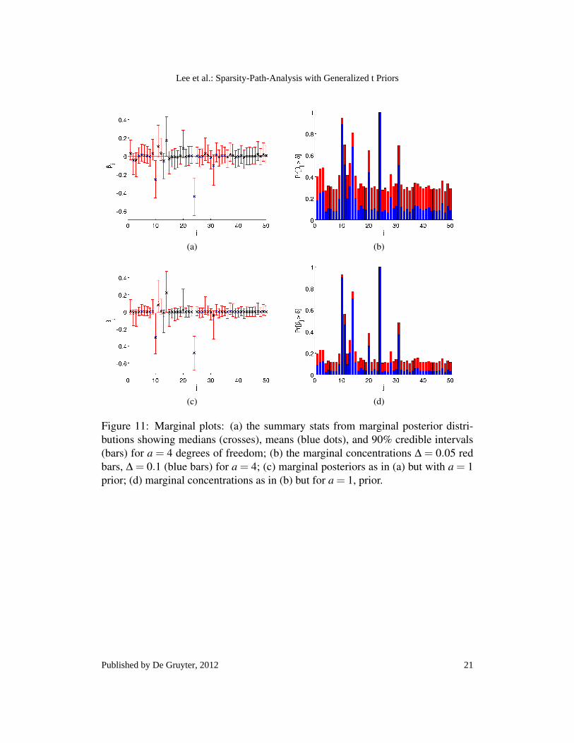
In Fig. 11 we plot summaries for the marginal posterior distributions of βββ as wellas the marginal concentrations, for a = 4 and a = 1. We can see in Fig. 11 that themarginal plots provide a useful overview of the relative importance of each variable.It may be difficult to distinguish the medians from the means in the visualization ofthe marginal posterior distributions on paper, but it is easy to see the difference ona computer screen.

20



(a) (b)

(c) (d)

Figure 11: Marginal plots: (a) the summary stats from marginal posterior distri-butions showing medians (crosses), means (blue dots), and 90% credible intervals(bars) for a = 4 degrees of freedom; (b) the marginal concentrations ∆ = 0.05 redbars, ∆ = 0.1 (blue bars) for a = 4; (c) marginal posteriors as in (a) but with a = 1prior; (d) marginal concentrations as in (b) but for a = 1, prior.

21



5.4 Comparison to double-exponential prior, a→ ∞

(a) MAPs (b) medians

(c) marginal density (d) concentrations

Figure 12: SPA plots for the double-exponential prior, Gt(a→ ∞,c).

It is informative to compare the results for the Gt(a,c) prior above withthat of the double-exponential prior p(β ) ∝ exp(−|β |/c) which is obtained as ageneralized t prior with q = 1 and a→ ∞. In Fig. 12 we show SPA plots for thiscase. We can see the much smoother paths of the MAP compared with Fig 4. Thiscan also be seen in the individual coefficient plots shown in Fig. 13 and Fig. 14. Itis interesting to investigate in more detail the posterior density of β24 the coefficientwith strongest evidence of association. This is shown in Fig. 15 and should becompared to Fig. 5 for a = 4. The concavity of the double-exponential prior causesthe posterior distribution to move smoothly towards being concentrated around 0 asc decreases, unlike the behaviour seen with the generalized t prior.

5.5 Large Data Set

We next analysed the larger data set with n = 1859 and p = 184. The indicesof the non-zero coefficients are I = {108,22,5,117,162} with the same valuesretained for βββI = {−0.2538,0.4578,−0.1873,−0.1498,0.0996}. The SPA plotsare shown in Fig. 16 with corresponding individual coefficient plots in Fig. 17 and

22



(a) double-exponential j = 14 (b) double-exponential j = 24

(c) double-exponential j = 31 (d) double-exponential j = 1

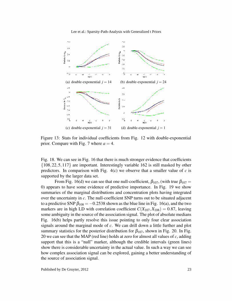
Figure 13: Stats for individual coefficients from Fig. 12 with double-exponentialprior. Compare with Fig. 7 where a = 4.

Fig. 18. We can see in Fig. 16 that there is much stronger evidence that coefficients{108,22,5,117} are important. Interestingly variable 162 is still masked by otherpredictors. In comparison with Fig. 4(c) we observe that a smaller value of c issupported by the larger data set.

From Fig. 16(d) we can see that one null-coefficient, β107, (with true β107 =0) appears to have some evidence of predictive importance. In Fig. 19 we showsummaries of the marginal distributions and concentration plots having integratedover the uncertainty in c. The null-coefficient SNP turns out to be situated adjacentto a predictive SNP β108 =−0.2538 shown as the blue line in Fig. 16(a), and the twomarkers are in high LD with correlation coefficient C(X107,X108) = 0.87, leavingsome ambiguity in the source of the association signal. The plot of absolute mediansFig. 16(b) helps partly resolve this issue pointing to only four clear associationsignals around the marginal mode of c. We can drill down a little further and plotsummary statistics for the posterior distribution for β107, shown in Fig. 20. In Fig.20 we can see that the MAP (red line) holds at zero for almost all values of c, addingsupport that this is a “null” marker, although the credible intervals (green lines)show there is considerable uncertainty in the actual value. In such a way we can seehow complex association signal can be explored, gaining a better understanding ofthe source of association signal.

23



(a) double-exponential j = 14 (b) double-exponential j = 24

(c) double-exponential j = 31 (d) double-exponential j = 1

Figure 14: Posterior density plots corresponding to Fig. 13 with double-exponentialprior.

Figure 15: Plot of marginal posterior of β24 as a function of c for double-exponentialprior a→ ∞. Under the double-exponential prior, a→ ∞, we see the posteriorremains log-concave and hence the MAP is a smooth function of logc; as comparedto Fig. 5.

24



(a) MAPs (b) medians

(c) marginal density (d) concentrations

Figure 16: SPA plots using the larger data set n = 1859, p = 184

6 DiscussionWe have presented an exploratory approach using generalized t priors that we callBayesian sparsity-path-analysis to aid in the understanding of genetic associationdata. The approach involves graphical summaries of posterior densities of coef-ficients obtained by sweeping over a range of prior precisions, including valueswith low posterior probability, in order to characterize the space of models from thesparse to the most complex.

This use of SMC methodology is ideally suited to the inference task, byindexing the SMC sampler on the scale of the prior. The resulting collection ofweighted particles provides us with approximations for the coefficient posteriordistributions for each scale in addition to estimates of the marginal likelihood andallows for improved robustness in MAP computation. The simulations are com-putationally demanding and would take days worth of run-time using conventionalsingle-threaded CPU processing. To alleviate this we make use of many-core GPUparallel processing producing around a 20-40 fold improvement in run-times. Thishas real benefit in allowing for data analysis within a working day for the largerdata set we considered.

25



(a) a = 4, j = 22 (b) a = 4, j = 5

(c) a = 4, j = 117 (d) a = 4, j = 115

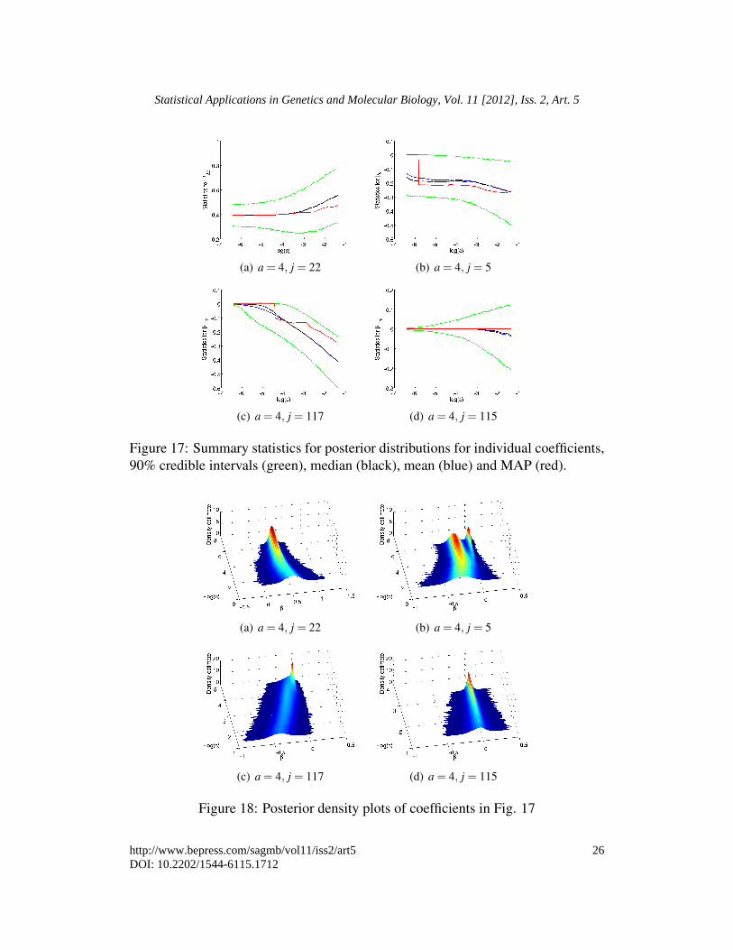
Figure 17: Summary statistics for posterior distributions for individual coefficients,90% credible intervals (green), median (black), mean (blue) and MAP (red).

(a) a = 4, j = 22 (b) a = 4, j = 5

(c) a = 4, j = 117 (d) a = 4, j = 115

Figure 18: Posterior density plots of coefficients in Fig. 17

26



(a) (b)

Figure 19: Marginal plots: (a) the summary stats from marginal posterior distri-butions showing medians (crosses), means (blue dots), and 90% credible intervals(bars) for a = 4 degrees of freedom; (b) the marginal concentrations ∆ = 0.05 redbars, ∆ = 0.1 (blue bars) for a = 4

Figure 20: Statistics for individual coefficient β107.

27



ReferencesArmagan, A., D. Dunson, and J. Lee (2011): “Generalized double Pareto shrink-

age,” ArXiv:1104.0861.Ayers, K. L. and H. J. Cordell (2010): “SNP selection in genome-wide and candi-

date gene studies via penalized logistic regression,” Genetic Epidemiology, 34,879–891.

Balding, D. J. (2006): “A tutorial on statistical methods for population associationstudies,” Nature Reviews Genetics, 7, 81–791.

Bornn, L., A. Doucet, and R. Gottardo (2010): “An efficient computational ap-proach for prior sensitivity analysis and cross-validation,” Canadian Journal ofStatistics, 38, 47–64.

Candes, E. J., M. B. Wakin, and S. P. Boyd (2008): “Enhancing sparsity byreweighted `1 minimization,” Journal of Fourier Analysis and Applications, 14,877–905.

Caron, F. and A. Doucet (2008): “Sparse bayesian nonparametric regression,” inProceedings of the 25th international conference on Machine learning, ACM,88–95.

Carvalho, C., N. Polson, and J. Scott (2010): “The horseshoe estimator for sparsesignals,” Biometrika, 97, 465.

Cevher, V. (2009): “Learning with compressible priors,” in Y. Bengio, D. Schuur-mans, J. Lafferty, C. K. I. Williams, and A. Culotta, eds., Advances in NeuralInformation Processing Systems 22, 261–269.

Chartrand, R. and W. Yin (2008): “Iteratively reweighted algorithms for compres-sive sensing,” in 33rd International Conference on Acoustics, Speech, and SignalProcessing (ICASSP).

Crooks, G. E. (1998): “Nonequilibrium measurements of free energy differ-ences for microscopically reversible Markovian systems,” Journal of StatisticalPhysics, 90, 1481–1487.

Del Moral, P., A. Doucet, and A. Jasra (2006): “Sequential Monte Carlo samplers,”Journal of the Royal Statistical Society B, 68, 411–436.

Del Moral, P., A. Doucet, and A. Jasra (2011): “An adaptive sequential Monte Carlomethod for approximate Bayesian computation,” Statistics and Computing, toappear.

Fan, J. and R. Li (2001): “Variable selection via nonconcave penalized likelihoodand its oracle properties,” Journal of the American Statistical Association, 96,1348–1360.

Fridley, B. (2009): “Bayesian variable and model selection methods for geneticassociation studies,” Genetic Epidemiology, 33, 27–37.

28



George, E. I. and R. E. McCulloch (1993): “Variable selection via Gibbs sampling,”Journal of the American Statistical Association, 88, 881–889.

Griffin, J. and P. Brown (2010): “Inference with normal-gamma prior distributionsin regression problems,” Bayesian Analysis, 5, 171–188.

Griffin, J. E. and P. J. Brown (2007): “Bayesian adaptive lassos with non-convexpenalization,” Technical report, IMSAS, University of Kent.

Hastie, T., R. Tibshirani, and J. Friedman (2009): The elements of statistical learn-ing: data mining, inference, and prediction, Springer Verlag.

Hoggart, C. J., J. C. Whittaker, M. De Iorio, and D. J. Balding (2008): “Simultane-ous analysis of all snps in genome-wide and re-sequencing association studies,”PLOS Genetics, 4, e1000130.

Lee, A., F. Caron, A. Doucet, and C. Holmes (2010a): “A hierarchical Bayesianframework for constructing sparsity-inducing priors,” ArXiv:1009.1914.

Lee, A., C. Yau, M. B. Giles, A. Doucet, and C. C. Holmes (2010b): “On theutility of graphics cards to perform massively parallel simulation of advancedMonte Carlo methods,” Journal of Computational and Graphical Statistics, 19,769–789.

Liu, J. S. and R. Chen (1995): “Blind deconvolution via sequential imputations,”Journal of the American Statistical Association, 90, 567–576.

McDonald, J. and W. Newey (1988): “Partially adaptive estimation of regressionmodels via the generalized t distribution,” Econometric Theory, 4, 428–457.

Neal, P. and G. Roberts (2006): “Optimal scaling for partially updating MCMCalgorithms,” Annals of Applied Probability, 16, 475–515.

Neal, R. M. (2001): “Annealed importance sampling,” Statistics and Computing,11, 125–139.

Park, T. and G. Casella (2008): “The Bayesian Lasso,” Journal of the AmericanStatistical Association, 103, 681–686.

Stephens, M. and D. Balding (2009): “Bayesian statistical methods for genetic as-sociation studies,” Nature Reviews Genetics, 10, 681–690.

Tibshirani, R. (1996): “Regression shrinkage and selection via the lasso,” Journalof the Royal Statistical Society B, 58, 267–288.

Tibshirani, R. (2011): “Regression shrinkage and selection via the lasso: a retro-spective,” Journal of the Royal Statistical Society B, 73, 273–282.

Wilson, M. A., E. S. Iversen, M. A. Clyde, S. C. Schmidler, and J. M. Schild-kraut (2010): “Bayesian model search and multilevel inference for snp associa-tion studies,” Annals of Applied Statistics, 4, 1342–1364.

Zou, H. (2006): “The adaptive lasso and its oracle properties,” Journal of the Amer-ican Statistical Association, 101, 1418–1429.

Zou, H. and R. Li (2008): “One-step sparse estimates in nonconcave penalizedlikelihood models,” Annals of Statistics, 36, 1509–1533.

29



Statistical Applications in Genetics and Molecular...

Documents

Transcript of Statistical Applications in Genetics and Molecular...