Statistical Applications in Genetics and Molecular...

Volume 10, Issue 1 2011 Article 28

Statistical Applications in Geneticsand Molecular Biology

The Joint Null Criterion for MultipleHypothesis Tests

Jeffrey T. Leek, Johns Hopkins Bloomberg School of PublicHealth

John D. Storey, Princeton University

Recommended Citation:Leek, Jeffrey T. and Storey, John D. (2011) "The Joint Null Criterion for Multiple HypothesisTests," Statistical Applications in Genetics and Molecular Biology: Vol. 10: Iss. 1, Article 28.DOI: 10.2202/1544-6115.1673Available at: http://www.bepress.com/sagmb/vol10/iss1/art28

©2011 Berkeley Electronic Press. All rights reserved.

The Joint Null Criterion for MultipleHypothesis Tests

Jeffrey T. Leek and John D. Storey

Abstract

Simultaneously performing many hypothesis tests is a problem commonly encountered inhigh-dimensional biology. In this setting, a large set of p-values is calculated from many relatedfeatures measured simultaneously. Classical statistics provides a criterion for defining what a“correct” p-value is when performing a single hypothesis test. We show here that even when eachp-value is marginally correct under this single hypothesis criterion, it may be the case that the jointbehavior of the entire set of p-values is problematic. On the other hand, there are cases where eachp-value is marginally incorrect, yet the joint distribution of the set of p-values is satisfactory. Here,we propose a criterion defining a well behaved set of simultaneously calculated p-values thatprovides precise control of common error rates and we introduce diagnostic procedures forassessing whether the criterion is satisfied with simulations. Multiple testing p-values that satisfyour new criterion avoid potentially large study specific errors, but also satisfy the usualassumptions for strong control of false discovery rates and family-wise error rates. We utilize thenew criterion and proposed diagnostics to investigate two common issues in high-dimensionalmultiple testing for genomics: dependent multiple hypothesis tests and pooled versus test-specificnull distributions.

KEYWORDS: false discovery rate, multiple testing dependence, pooled null statistics

1 IntroductionSimultaneously performing thousands or more hypothesis tests is one of the maindata analytic procedures applied in high-dimensional biology (Storey and Tibshi-rani, 2003). In hypothesis testing, a test statistic is formed based on the observeddata and then it is compared to a null distribution to form a p-value. A fundamentalproperty of a statistical hypothesis test is that correctly formed p-values follow theUniform(0,1) distribution for continuous data when the null hypothesis is true andsimple. (We hereafter abbreviate this distribution by U(0,1).) This property allowsfor precise, unbiased evaluation of error rates and statistical evidence in favor ofthe alternative. Until now there has been no analogous criterion when performingthousands to millions of tests simultaneously.

Just as with a single hypothesis test, the behavior under true null hypothe-ses is the primary consideration in defining well behaved p-values. However, whenperforming multiple tests, the situation is more complicated for several reasons: (1)among the entire set of hypothesis tests, a subset are true null hypotheses and theremaining subset are true alternative hypotheses, and the behavior of the p-valuesmay depend on this configuration; (2) the data from each true null hypothesis mayfollow a different null distribution; (3) the data across hypothesis tests may be de-pendent; and (4) the entire set of p-values is typically utilized to make a decisionabout significance, some of which will come from true alternative hypotheses. Be-cause of this, it is not possible to simply extrapolate the definition of a correctp-value in a single hypothesis test to that of multiple hypothesis tests. We providetwo key examples to illustrate this point in the following section, both of which arecommonly encountered in high-dimensional biology applications.

The first major point of this paper is that the joint distribution of the truenull p-values is a highly informative property to consider, whereas verifying thateach null p-value has a marginal U(0,1) distribution is not as directly informative.We propose a new criterion for null p-values from multiple hypothesis tests thatguarantees a well behaved joint distribution, called the Joint Null Criterion (JNC).The criterion is that the ordered null p-values are equivalent in distribution to thecorresponding order statistics of a sample of the same size from independent U(0,1)distributions. We show that multiple testing p-values that satisfy our new criterioncan be used to more precisely estimate error rates and rank tests for significance. Weillustrate with simple examples how this criterion avoids potentially unacceptablelevels of inter-study variation that is possible even for multiple testing proceduresthat guarantee strong control.

The second major point of this paper is that new diagnostics are needed toobjectively compare various approaches to multiple testing, specifically those thatevaluate properties beyond control of expected error rate estimates over repeated

1

Leek and Storey: Joint Null Criterion

Published by Berkeley Electronic Press, 2011

studies. These new diagnostics should also be concerned with potentially largestudy specific effects that manifest over repeated studies in terms of the varianceof realized error rates (e.g., the false discovery proportion) and the variance of er-ror rate estimates. This has been recognized as a particularly problematic in thecase of dependent hypothesis tests where unacceptable levels of variability in er-ror rate estimates may be obtained even though the false discovery rate may becontrolled (Owen, 2005). The need for this type of diagnostic is illustrated in anexample presented in the next section, where the analysis of gene expression uti-lizing three different approaches yields drastically different answers. We proposeBayesian and frequentist diagnostic procedures that provide an unbiased standardfor null p-values from multiple testing procedures for complex data. When appliedto these methods, the reasons for their differing answers are made clearer.

We apply our diagnostics to the null p-values from multiple simulated stud-ies, to capture the potential for study specific errors. We use the diagnostics toevaluate methods in two major areas of current research in multiple testing: testingmultiple dependent hypotheses and pooled versus test-specific null distributions.Surprisingly, some popular multiple testing procedures do not produce p-valueswith a well behaved joint null distribution, leading directly to imprecise estimatesof common error rates such as the false discovery rate.

2 Motivating ExamplesHere we motivate the need for the JNC and diagnostic tests by providing two gen-eral examples and a real data example from a gene expression study. The firstgeneral example describes a situation where every p-value has a U(0,1) distribu-tion marginally over repeated studies. However, the joint distribution of study-specific sets of null p-values deviate strongly from that of independent U(0,1) com-ponents. The second general example illustrates the opposite scenario: here noneof the p-values has a U(0,1) distribution marginally, but the set of study-specificnull p-values appear to have a joint distribution equivalent to independent U(0,1)components of the same size. Together, these examples suggest the need for a goldstandard for evaluating multiple testing procedures in practice. Finally, we showthat different methods for addressing multiple testing dependence give dramaticallydifferent results for the same microarray analysis. This indicates that an objectivecriterion is needed for evaluating such methods in realistic simulations where thecorrect answer is known.

2

Statistical Applications in Genetics and Molecular Biology, Vol. 10 [2011], Iss. 1, Art. 28

http://www.bepress.com/sagmb/vol10/iss1/art28DOI: 10.2202/1544-6115.1673

2.1 Problematic Joint Distribution from Correct Marginal Dis-tributions

In this example, the goal is to test each feature for a mean difference between twogroups of equal size. The first 300 features are simulated to have a true meandifference. There is also a second, randomized unmodeled binary variable thataffects the data. Features 200-700 are simulated to have a mean difference betweenthe groups defined by the unmodeled variable. The exact model and parameters forthis simulation are detailed in Section 5. The result of performing these tests is a1,000 × 100 matrix of p-values, where the p-values for a single study appear incolumns and the p-values for a single test across repeated studies appear in rows.

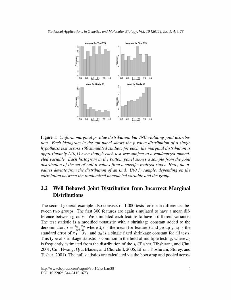
Using these p-values we examine both their marginal distributions as well asthe joint distribution of the null p-values. First, we look at a single p-value affectedby the unmodeled variable over the 100 repeated studies. The top two histograms inFigure 1 show the behavior of two specific p-values over the 100 simulated studies.Marginally, each is U(0,1) distributed as would be expected. The randomizationof the unmodeled variable results in correct marginal distributions for each nullp-value.

Next we consider the null p-values from tests 301-700 for a single study,which is a sample from their joint distribution. The bottom two histograms in Fig-ure 1 show two such examples. In one case the null p-values appear smaller thanexpected from an i.i.d. U(0,1) sample, in the other case they appear to be largerthan expected. This is because in the first study, the unmodeled variable is cor-related with the group difference and the signal from the unmodeled variable isdetected by the test between groups. In the second study, the unmodeled variable isuncorrelated with the group difference and a consistent source of noise is added tothe data, resulting in null p-values that are too large. The result is that each null p-value is U(0,1) marginally, but the joint distribution deviates strongly from a sampleof i.i.d. U(0,1) random variables.

Of particular interest is the lower left histogram of Figure 1, which showsonly the null p-values from a single simulated study with dependence. The p-valuesappear to follow the usual pattern of differential expression, with some p-valuesnear zero (ostensibly corresponding to differential expressed genes) and some p-values that appear to be drawn from a U(0,1) distribution (ostensibly the null genes).However, in this example all of the genes are true nulls, so ideally their joint dis-tribution would reflect the U(0,1). Inspection of this histogram would lead to themistaken conclusion that the method had performed accurately and true differentialexpression had been detected. This strongly motivates the need for new diagnostictools that consider the joint behavior of null p-values.

3



Marginal for Test 778

P−value

Fre

quen

cy0.0 0.2 0.4 0.6 0.8 1.0

02

46

810

12


P−value

Fre

quen

cy

0.0 0.2 0.4 0.6 0.8 1.0

05

1015

Joint for Study 78

P−value

Fre

quen

cy

0.0 0.2 0.4 0.6 0.8 1.0

050

100

150

Joint for Study 50

P−value

Fre

quen

cy0.0 0.2 0.4 0.6 0.8 1.0

020

4060

80

Figure 1: Uniform marginal p-value distribution, but JNC violating joint distribu-tion. Each histogram in the top panel shows the p-value distribution of a singlehypothesis test across 100 simulated studies; for each, the marginal distribution isapproximately U(0,1) even though each test was subject to a randomized unmod-eled variable. Each histogram in the bottom panel shows a sample from the jointdistribution of the set of null p-values from a specific realized study. Here, the p-values deviate from the distribution of an i.i.d. U(0,1) sample, depending on thecorrelation between the randomized unmodeled variable and the group.

2.2 Well Behaved Joint Distribution from Incorrect MarginalDistributions

The second general example also consists of 1,000 tests for mean differences be-tween two groups. The first 300 features are again simulated to have a mean dif-ference between groups. We simulated each feature to have a different variance.The test statistic is a modified t-statistic with a shrinkage constant added to thedenominator: t = xi1−xi0

si+a0where xi j is the mean for feature i and group j, si is the

standard error of xi1− xi0, and a0 is a single fixed shrinkage constant for all tests.This type of shrinkage statistic is common in the field of multiple testing, where a0is frequently estimated from the distribution of the si (Tusher, Tibshirani, and Chu,2001, Cui, Hwang, Qiu, Blades, and Churchill, 2005, Efron, Tibshirani, Storey, andTusher, 2001). The null statistics are calculated via the bootstrap and pooled across

4



features (Storey and Tibshirani, 2003). The top row of Figure 2 shows the distribu-tion of two specific p-values across the 100 studies. In this case, since the standarderrors vary across tests, the impact a0 has on the test’s null distribution depends onthe relative size of a0 to the si.

When the null statistics are pooled, there are individual tests whose p-valuefollows an incorrect marginal distribution across repeated studies. The reason isthat the bootstrap null statistics are pooled across 1,000 different null distributions.The bottom row of Figure 2 shows a sample from the joint distribution of the nullp-values for specific studies. The joint distribution behaves like an i.i.d. U(0,1)sample because pooling the bootstrap null statistics captures the overall impact ofdifferent variances on the joint distribution of the test statistics coming from truenull hypotheses.


P−value

Fre

quen

cy

0.0 0.2 0.4 0.6 0.8 1.0

05

1015


P−value

Fre

quen

cy

0.0 0.2 0.4 0.6 0.8 1.0

05

1015

Joint for Study 83

P−value

Fre

quen

cy

0.0 0.2 0.4 0.6 0.8 1.0

010

2030

4050

Joint for Study 80

P−value

Fre

quen

cy

0.0 0.2 0.4 0.6 0.8 1.0

010

2030

4050

60

Figure 2: Non-uniform marginal p-value distribution, but JNC satisfying joint dis-tribution. Each histogram in the top panel shows the p-value distribution of a sin-gle hypothesis test using a shrunken t-statistic and pooled null statistics across 100simulated studies. It can be seen in each that the marginal distribution deviatesfrom U(0,1). Each histogram in the bottom panel shows a sample from the jointdistribution of the set of null p-values from two specific realizations of the study.Here, the p-values satisfy the JNC, since pooling the null statistics accounts for thedistribution of variances across tests.

5



2.3 Microarray Significance Analysis

Idaghdour, Storey, Jadallah, and Gibson (2008) performed a study of 46 desertnomadic, mountain agrarian, and coastal urban Moroccan Amazigh individuals toidentify differentially expressed genes across geographic populations. Due to theheterogeneity of these groups and the observational nature of the study, there islikely to be latent structure present in the data, leading to multiple testing depen-dence. This can be easily verified by examining the residual data after regressingout the variables of interest (Idaghdour et al., 2008). As an example we present twodifferential expression analyses in Figure 3: agrarian versus desert nomadic, anddesert nomadic versus village.

P!value

Frequency

0.0 0.2 0.4 0.6 0.8 1.0

01000

2000

3000

P!value

Frequency

0.0 0.2 0.4 0.6 0.8 1.0

01000

2000

3000

P!value

Frequency

0.0 0.2 0.4 0.6 0.8 1.0

01000

2000

3000

P!value

Frequency

0.0 0.2 0.4 0.6 0.8 1.0

01000

2000

3000

P!value

Frequency

0.0 0.2 0.4 0.6 0.8 1.0

01000

2000

3000

P!value

Frequency

0.0 0.2 0.4 0.6 0.8 1.0

01000

2000

3000

!"#$#%$&''

()*'

+,),#-'

+,),#-'

()*'

.%//$",'

01-,)-' 23##4"$-,'.$#%$5/,'' 678%#%9$/':3//'

Figure 3: P-value histograms from the differential expression analysis comparingagrarian versus desert nomadic (top row) and desert nomadic versus village (bot-tom row). For each comparison, three different analysis strategies are used: a stan-dard F-statistic significance (first column), a surrogate variable adjusted approach(second column), and an empirical null adjusted approach (third column). The lasttwo are methods for adjusting for multiple testing dependence. Both comparisonsshow wildly different results depending on the analysis technique used.

We perform each analysis in three ways, (1) a simple F-test for comparinggroup means, (2) a surrogate variable adjusted analysis (Leek and Storey, 2007),and (3) an empirical null (Efron, 2004, 2007) adjusted analysis. These last two ap-proaches are different methods for adjusting for multiple testing dependence and

6



latent structure in microarray data. Figure 3 shows that each analysis strategy re-sults in a very different distribution for the resulting p-values. Idaghdour et al.(2008) found coherent and reproducible biology among the various comparisonsonly when applying the surrogate variable analysis technique. However, how dowe know in a more general sense which, if any, of these analysis strategies is morewell behaved since they give such different results? This question motivates a needfor a criterion and diagnostic test for evaluating the operating characteristics multi-ple testing procedures, where the criterion is applied to realistically simulated datawhere the correct answers are known.

3 A Criterion for the Joint Null DistributionThe examples from the previous section illustrate that it is possible for p-valuesfrom multiple tests to have proper marginal distributions, but together form a prob-lematic joint distribution. It is also possible to have a well behaved joint distribu-tion, but composed of p-values with incorrect marginal distributions. In practiceonly a single study is performed and the statistical significance is assessed from theentire set of p-values from that study. The real data example shows that differentmethods may yield notably different p-value distributions in a given study.

Thus, utilizing a procedure that produces a well behaved joint distributionof null p-values is critical to reduce deviation from uniformity of p-values withina study, and large variances of statistical significance across studies. A single hy-pothesis test p-value is correctly specified if its distribution is U(0,1) under thenull (Lehmann, 1997). In other words, p is correctly specified if for α ∈ (0,1),Pr(p < α) = Pr(U < α) = α , where U ∼U(0,1). We would like to ensure that thenull p-values from a given experiment have a joint distribution that is stochasticallyequivalent to an independent sample from the U(0,1) distribution of the same size.Based on this intuition, we propose the following criterion for the joint null p-valuedistribution.

Definition (Joint Null Criterion, JNC). Suppose that m hypothesis tests are per-formed where tests 1,2, . . . ,m0 are true nulls and m0+1, . . . ,m are true alternatives.Let pi be the p-value for test i and let p(ni) be the order statistic corresponding topi among all p-values, so that ni = #{p j ≤ pi}. The set of null p-values satisfy theJoint Null Criterion if and only if the joint distribution of p(ni), i = 1, . . . ,m0 is equalto the joint distribution of p∗(n∗i )

, i = 1, . . . ,m0, where p∗1, . . . , p∗m0are an i.i.d. sample

from the U(0,1) distribution and p∗ia.s.= pi, for i = m0 +1, . . . ,m.

7



Remark 1. If all the p-values correspond to true nulls, the JNC is equivalent tosaying that the ordered p-values have the same distribution as the order statisticsfrom an i.i.d. sample of size m from the U(0,1) distribution. �

Intuitively, when the JNC is satisfied and a large number of hypothesis testsis performed, the set of null p-values from these tests should appear to be equivalentto an i.i.d. sample from the U(0,1) distribution when plotted together in a histogramor quantile-quantile plot. Figure 4 illustrates the conceptual difference between theJNC and the univariate criterion. The p-values from multiple tests for a singlestudy appear in columns and the p-values from a single test across studies appearin rows. The standard univariate criterion is concerned with the behavior of singlep-values across multiple studies, represented as rows in Figure 4. In contrast, theJNC is concerned with the joint distribution of the set of study-specific p-values,represented by columns in Figure 4. When only a single test is preformed, eachcolumn has only a single p-value so the JNC is simply the standard single testcriterion.

Remark 2. In the case that the null hypotheses are composite, the distributionalequality in the above criterion can be replaced with a stochastic ordering of the twodistributions. �

Remark 3. The JNC is not equivalent to the trivial case where the null p-valuesare each marginally U(0,1) and they are jointly independent. Let U(1) ≤ U(2) ≤·· · ≤U(m0) be the order statistics from an i.i.d. sample of size m0 from the U(0,1)distribution. Set pi = U(i) for i = 1, . . . ,m0. It then follows that the null p-valuesare highly dependent (since pi < p j for all i < j), none are marginally U(0,1), buttheir joint distribution is valid. Example 2 from Section 2 provides another scenariowhere the JNC is not equivalent to the trivial case. �

Remark 4. The JNC is not a necessary condition for the control of the false dis-covery rate, as it has been shown that the false discovery rate may be controlledfor certain types of dependence that may violate the JNC (Benjamini and Yekutieli,2001, Storey, Taylor, and Siegmund, 2004). �

The JNC places a condition on the joint behavior of the set of null p-values.This joint behavior is critical, since error estimates and significance calculation areperformed on the set of p-values from a single study (e.g., false discovery ratesestimates Storey (2002)). To make this concrete, consider the examples from theprevious section. In Example 1, the joint distribution of the null p-values is muchmore variable than a sample from the U(0,1) distribution, resulting in unreliableerror rate estimates and significance calculations (Owen, 2005). The joint p-valuesin this example fail to meet the JNC. In Example 2, the joint distribution of the

8



!"#$%&'(")*+,-)(#$#"-(#-"%.''""

+/01'.("$#"2,33(2-"4)(%"513&$%1''*"

6789:;"123,##"3(+'$21-(<"#-.<$(#="

>.'?+'(")*+,-)(#$#"-(#-"%.''""

+/01'.(#"#1?#@*"-)("ABC"4)(%"

-)(*"13("(D.$01'(%-"-,"1%"$=$=<="

#15+'("@3,5"6789:;"123,##"

#-.<$(#="

!"#$%&'(")*+(,)%"+*

-,$(%#$"*

(!,"*.,$$*

/0#1(/"+%+*

("+(+*

Figure 4: An illustration of the Joint Null Criterion. The p-values from multipletests for a single study appear in columns and the p-value from a single test acrossreplicated studies compose each row. The JNC evaluates the joint distribution ofthe set of null p-values, whereas the single test criterion is concerned with the dis-tribution of a single p-value across replicated studies.

p-values satisfies the JNC, resulting in well behaved error rate estimates and sig-nificance calculations, even though the marginal behavior of each p-value is notU(0,1).

When the JNC is met, then estimation of experiment-wide error rates andsignificance cutoffs behaves similarly to the well behaved situation where the truenull p-values are i.i.d. U(0,1). Lemma 1 makes these ideas concrete (see Supple-mentary Information for the proof).

Lemma 1 Suppose that p1, p2, . . . , pm are m p-values resulting from m hypothesistests; without loss of generality, suppose that p1, . . . , pm0 correspond to true nullhypotheses and pm0+1, . . . , pm to true alternative hypotheses. If (1) the JNC is sat-isfied for p1, . . . , pm0 and (2) the conditional distribution {p(ni)}

mi=m0+1|{p(ni)}

m0i=1

9



is equal to the conditional distribution {p∗(ni)}m

i=m0+1|{p∗(ni)}m0

i=1, then any multiplehypothesis testing procedure based on the order statistics p(1), . . . , p(m) has prop-erties equivalent to those in the case where the true null hypotheses’ p-values arei.i.d. Uniform(0,1).

Corollary. When conditions (1) and (2) of Lemma 1 are satisfied, the multipletesting procedures of Shaffer (1995), Benjamini and Hochberg (1995), Storey et al.(2004) provide strong control of the false discovery rate. Furthermore, the control-ling and estimation properties of any multiple testing procedure requiring the nullp-values to be i.i.d. Uniform(0,1) continue to hold true when the JNC is satisfied.

The Joint Null Criterion is related to two well-known concepts in multipletesting, the marginal determine joint (MDJ) condition (Xu and Hsu, 2007, Calian,Li, and Hsu, 2008) and the joint null domination (jtNDT) condition (Dudoit andvan der Laan, 2008). The MDJ is a condition on the observations, which is sufficientto guarantee a permutation distribution is the same as the true distribution (Calianet al., 2008). Meanwhile, the jtNDT condition is concerned with Type I errorsbeing stochastically greater under the test statistics null distribution than under theirtrue distribution. From this, Dudoit and van der Laan (2008) show that two maintypes of null distributions for test statistics can be constructed that satisfy this nulldomination property. The difference between these criteria and the JNC is that theJNC focuses not just one Type I error control, but also controlling the study-to-studyvariability in Type I errors.

4 Statistical Methods for Evaluating the Joint NullCriterion

Several new multiple testing statistics for the analysis of gene expression data haverecently been proposed and evaluated in the literature (Tusher et al., 2001, Newton,Noueiry, Sarkar, and Ahlquist, 2004, Storey, 2007). A standard evaluation of theaccuracy of a new procedure is to apply it to simulated data and determine whethera particular error rate, such as the false discovery rate, is conservatively biased atspecific thresholds, typically 5% and 10%. The JNC suggests a need for methodsto evaluate the joint distribution of null p-values from multiple testing procedures.We propose a three step approach for evaluating whether the joint distribution ofnull p-values satisfies the JNC.

1. Simulate multiple high-dimensional data sets from a common data generat-ing mechanism that captures the expected cross study variation in signal andnoise, and includes any dependence or latent structure that may be present.

10



2. Apply the method(s) in question to each study individually to produce a setof p-values for each study.

3. Compare the set of null p-values from each specific study to the U(0,1) dis-tribution, and quantify differences between the two distributions across allstudies.

The first two steps of our approach involve simulating data and applyingthe method in question to generate p-values, which we carry out in the next sectionin the context of multiple testing dependence and pooling null distributions acrosstests. When the joint null distribution can be characterized directly (Huang, Xu,Calian, and Hsu, 2006), analytic evaluation of the JNC may be possible. A keycomponent of evaluating the JNC is the ability to simulate from a realistic jointdistribution for the observed data. Application of these diagnostic criteria requirescareful examination of the potential properties, artifacts, and sources of dependencethat exist in high-dimensional data. In the remainder of the current section, we pro-pose methods for the third step: summarizing and evaluating null p-values relativeto the U(0,1) distribution.

We propose one non-parametric approach based on the Kolmogorov-Smirnov(KS) test and a second approach based on a Bayesian posterior probability for thejoint distribution. When applying these diagnostics to evaluate multiple testing pro-cedures that produce a small number of observed p-values (m< 100) the asymptoticproperties of the KS test may not hold. For these scenarios, the Bayesian diagnosticmay be more appropriate. In the more general case, when a large number of testsare performed, the diagnostics are both appropriate.

4.1 Double Kolmogorov-Smirnov Test

In this step we start with m p-values from B simulated studies, p1 j, . . . , pm j, j =1, . . .B. Assume that the first m0 p-values correspond to the null tests and the lastm−m0 correspond to the alternative tests. To directly compare the behavior of thep-values from any study to the U(0,1) distribution, we consider the study-specificempirical distribution function, defined for study j as F j

m0(x) =1

m0∑

m0i=1 1(pi j < x).

The empirical distribution is an estimate of the unknown true distribution of thenull p-values F j(x). If the null p-values are U(0,1) distributed then F j

m0(x) willbe close to the U(0,1) distribution function, F(x) = x. In practice, none of theempirical distribution functions will exactly match the U(0,1) distribution due torandom variation.

One approach to determine if the p-values are “close enough” to the U(0,1)distribution is to perform a KS test (Shorack and Wellner, 1986) using the statistic,D j

m0 = supx |Fj

m0(x)−x| (see also Supplementary Figure S1). Based on this statistic

11



we can calculate a KS test p-value for each simulated study. Under the null hypoth-esis the KS tests’ p-values will also be U(0,1) distributed. We can then calculate asecond KS test statistic based on the empirical distribution of the first stage KS testp-values. If the original test-specific null p-values are U(0,1) distributed, then thisdouble KS test p-value will be large and if not then it will be small. Repeating theKS test across a range of simulated data sets permits us to quantify variation aroundthe U(0,1) distribution. Replication also reduces the potential for getting lucky andpicking a single simulated study where the method in question excels.

Note that it is possible to consider metrics less stringent than the supremumnorm on which the KS test is based. There are variety of ways in which a metricbased on |F j

m0(x)− x| over the range 0≤ x≤ 1 can be calculated.

4.2 Bayesian Posterior Probability

A second approach we propose for evaluating the joint distribution of the null p-values is to estimate the posterior probability that the JNC holds given the sets ofm p-values across the B simulated studies. To calculate this posterior probability,we assume that the observed null p-values are drawn from a flexible class of distri-butions. For example, we assume the null p-values are a sample from a Beta(α,β )distribution, where (α,β ) ∈ [0,A]× [0,B]. Supplementary Figure S2 shows exam-ples of the density functions for a range of values of (α,β ). The Beta family isused because Beta distributions closely mimic the behavior of non-null p-valuesobserved in practice (Pounds and Morris, 2003). For example, if α = 1 and β > 1then the corresponding Beta density function is strictly decreasing between 0 and 1,which is typical of the distribution of p-values from differentially expressed genesin a microarray experiment.

Our approach assigns prior probability 1/2 that the p-values are jointly U(0,1)(i.e., the JNC holds), equivalent to a Beta distribution with α = β = 1, and priorprobability 1/2 that the p-values follow a Beta distribution where either α 6= 1 orβ 6= 1. We write {pi j} as shorthand for the entire set of simulated null p-values,{pi j; i = 1, . . . ,m0, j = 1, . . . ,B}. From Bayes Theorem we can calculate the poste-rior probability the JNC holds as follows:

Pr(JNC holds |{pi j})

=12Pr({pi j}|JNC holds)

12Pr({pi j}|JNC holds)+ 1

2Pr({pi j}|JNC does not hold).

12



The first component is calculated as:

Pr({pi j}|JNC holds) = Pr({pi j}|(α,β ) = 1) =m0

∏i=1

B

∏j=1

1(0≤ p ji ≤ 1) = 1.

The second component can be calculated by integrating over the other values of(α,β ):

Pr({pi j}|JNC does not hold)

=∫ A

0

∫ B

0

m0

∏i=1

B

∏j=1

Γ(α +β )

Γ(α)Γ(β )pα−1

i j (1− pi j)β−1

π0(α,β )dαdβ

where π0(α,β ) is the prior distribution for specific values of (α,β ). In the exam-ples that follow, we utilize independent U(0,1) priors on both α and β , but moreinformative prior choices could be used to emphasize specific potential alternatives.For example, weighting the prior toward values with α < 1 and β > 1 would em-phasize distributions that are stochastically smaller than the U(0,1) distribution andtypically occur under the alternative.

5 Applications of the Joint Null CriterionWe apply the proposed JNC and diagnostic tests to assess the behavior of methodsor two important challenges in multiple hypothesis testing: (1) addressing multi-ple testing dependence and (2) determining the validity pooled null distributions.Methods have been developed for both of these issues in multiple testing, but therehas not been a standard approach for evaluating whether the resulting significancemeasures have desirable variability properties.

5.1 Multiple Testing Dependence

Multiple testing dependence is a common problem in the analysis of high-dimensionaldata such as those obtained from genomics (Leek and Storey, 2007) or imagingexperiments (Schwartzman, Dougherty, and Taylor, 2008). Multiple testing depen-dence has frequently been defined as a type of stochastic dependence among p-values or one-dimensional test-statistics when performing multiple tests (Yekutieliand Benjamini, 1999, Benjamini and Yekutieli, 2001, Efron, 2004, 2007). More re-cently, the root source of this type of dependence has been identified and addressedas dependence among the data for the tests (Leek and Storey, 2008). It has alsobeen shown that regardless of the dependence structure, dependence in the feature

13



level data can always be parameterized by a low dimensional set of variables (orfactors) called a dependence kernel (Leek and Storey, 2008).

Three different approaches for addressing multiple testing dependence are:surrogate variable analysis (Leek and Storey, 2007, 2008), residual factor analysisfor multiple testing dependence (Friguet, Kloareg, and Causer, 2009), and the em-pirical null (Efron, 2004) as applied to multiple testing dependence (Efron, 2007).Surrogate variable analysis is an approach that performs a supervised factor anal-ysis of the data during the modeling process, before one dimensional summariessuch as p-values have been calculated. Residual factor analysis for multiple test-ing dependence is a reformulation of this approach where the estimated factors arerequired to be orthogonal to the class variable. The empirical null distribution iscalculated based on the observed values of the test statistics. The basic idea is to es-timate a null distribution based on the “null part” of the observed distribution wherethe null statistics are assumed to lie. We note that the empirical null method as ageneral approach (Efron, 2004, 2007) has not been subjected to simulations wherethe correct answer is known, so its accuracy and general operating characteristicsare heretofore unexplored.

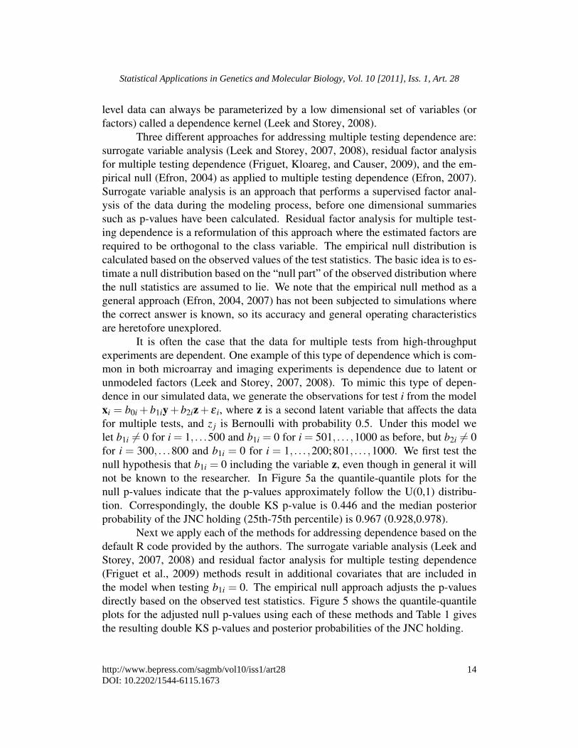
It is often the case that the data for multiple tests from high-throughputexperiments are dependent. One example of this type of dependence which is com-mon in both microarray and imaging experiments is dependence due to latent orunmodeled factors (Leek and Storey, 2007, 2008). To mimic this type of depen-dence in our simulated data, we generate the observations for test i from the modelxi = b0i + b1iy+ b2iz+ ε i, where z is a second latent variable that affects the datafor multiple tests, and z j is Bernoulli with probability 0.5. Under this model welet b1i 6= 0 for i = 1, . . .500 and b1i = 0 for i = 501, . . . ,1000 as before, but b2i 6= 0for i = 300, . . .800 and b1i = 0 for i = 1, . . . ,200;801, . . . ,1000. We first test thenull hypothesis that b1i = 0 including the variable z, even though in general it willnot be known to the researcher. In Figure 5a the quantile-quantile plots for thenull p-values indicate that the p-values approximately follow the U(0,1) distribu-tion. Correspondingly, the double KS p-value is 0.446 and the median posteriorprobability of the JNC holding (25th-75th percentile) is 0.967 (0.928,0.978).

Next we apply each of the methods for addressing dependence based on thedefault R code provided by the authors. The surrogate variable analysis (Leek andStorey, 2007, 2008) and residual factor analysis for multiple testing dependence(Friguet et al., 2009) methods result in additional covariates that are included inthe model when testing b1i = 0. The empirical null approach adjusts the p-valuesdirectly based on the observed test statistics. Figure 5 shows the quantile-quantileplots for the adjusted null p-values using each of these methods and Table 1 givesthe resulting double KS p-values and posterior probabilities of the JNC holding.

14



0.0 0.2 0.4 0.6 0.8 1.00.

00.

20.

40.

60.

81.

0

Uniform Quantiles

Em

piric

al Q

uant

iles

a

0.0 0.2 0.4 0.6 0.8 1.0

0.0

0.2

0.4

0.6

0.8

1.0

Uniform Quantiles

Em

piric

al Q

uant

iles

b

0.0 0.2 0.4 0.6 0.8 1.0

0.0

0.2

0.4

0.6

0.8

1.0

Uniform Quantiles

Em

piric

al Q

uant

iles

c

0.0 0.2 0.4 0.6 0.8 1.00.

00.

20.

40.

60.

81.

0

Uniform Quantiles

Em

piric

al Q

uant

iles

d

Figure 5: Quantile-quantile plots of the joint distribution of null p-values from 100simulated studies when the hypothesis tests are dependent. Results when utilizing:a. the true latent variable adjustment, b. surrogate variable analysis, c. empiricalnull adjustment, and d. residual factor analysis.

part like the correctly adjusted p-values in Figure 5a, with the exception of a smallnumber of cases, where the unmodeled variable is nearly perfectly correlated withthe group difference. The resulting posterior probability estimates are consistentlynear 1; however, the double KS p-value is sensitive to the small number of outlyingobservations.

The empirical null adjustment shows a strong conservative bias, which re-sults in a loss of power (Figure 5c). The reason appears to be that the estimatedempirical null is often too wide due to the extreme statistics from the dependencestructure. Since the one-dimensional summary statistics conflate signal and noise, itis generally impossible to estimate the null distribution well in the case of dependentdata. It has been recommended that the empirical null be employed only when theproportion of truly null hypotheses is greater than 0.90, potentially because of thisbehavior. Under this assumption, the null p-values are somewhat closer to U(0,1),but still show strong deviations in many cases (Table 1). This indicates the empiri-cal null may be appropriate in limited scenarios when only a small number of testsare truly alternative, such as in genome-wide association studies as originally sug-

The surrogate variable adjusted p-values (Figure 5b) behave for the most

15



or brain imaging studies.The residual factor analysis adjusted null p-values, where the factors are

required to be orthogonal to the group difference, show strong anti-conservative bias(Figure 5d). The reason is that the orthogonally estimated factors do not accountfor potential confounding between the tested variable and the unmodeled variable.However, when the unmodeled variable is nearly orthogonal to the group variableby chance, this approach behaves reasonably well and so the 75th percentile of theposterior probability estimates is 0.810.

Table 1: The posterior probability distribution and the double KS test p-value as-sessing whether the JNC holds for each method adjusting for multiple testing de-pendence. Correctly Adjusted = adjusted for the true underlying latent variable,SV = surrogate variable analysis, EN = empirical null, and RF = residual factoranalysis.

Method Post. Prob. (IQR) dKS P-valueCorrectly Adjusted 0.967 (0.928,0.978) 0.446SV Adjusted 0.961 (0.918,0.975) 0.132EN Adjusted 0.000 (0.000,0.000) < 2e-16EN Adjusted (95% Null) 0.685 (0.081,0.961) 1.443e-14RF Adjusted 0.000 (0.000,0.810) < 2e-16

Supplementary Figures S3 and S4 show the estimates of the FDR and theproportion of true nulls calculated for the same simulated studies. Again, the es-timates using the correct model and surrogate variable analysis perform similarly,while the empirical null estimates are conservatively biased and the residual factoranalysis p-values are anti-conservatively biased. For comparison purposes, Supple-mentary Figure S5 shows the behavior of the unadjusted p-values and their corre-sponding false discovery rate estimates. It can be seen that since surrogate variablesanalysis satisfies the JNC, it produces false discovery rate estimates with a varianceand a conservative bias close to the correct adjustment. However, the empirical nulladjustment and residual factor analysis produce substantially biased estimates. Theunadjusted analysis produces estimates with a similar expected value to the correctadjustment, although the variances are very large.

Another way to view this analysis is to consider the sensitivity and speci-ficity of each approach. The ROC curves for each of the four proposed methodsare shown in Supplementary Figure S6. The approaches that pass the JNC criteria- the correctly adjusted analysis and the surrogate variable adjusted analysis - have

gested by Devlin and Roeder (1999) – but not for typical microarray, sequencing,

16



similarly high AUC values, while the approaches that do not pass the JNC (residualfactor analysis and empirical null) have much lower AUC values. This suggeststhat another property of the JNC is increased sensitivity and specificity of multipletesting procedures.

5.2 Pooled Null Distributions

A second challenge encountered in large-scale multiple testing in genomics is indetermining whether it is valid to form an averaged (called “pooled”) null distribu-tion across multiple tests. Bootstrap and permutation null distributions are commonfor high-dimensional data, where parametric assumptions may be difficult to ver-ify. It is often computationally expensive to generate enough null statistics to maketest-specific empirical p-values at a fine enough resolution. (This requires at leastas many resampling iterations as there are tests.) One proposed solution is to poolthe resampling based null statistics across tests when forming p-values or estimat-ing other error rates (Tusher et al., 2001, Storey and Tibshirani, 2003). By poolingthe null statistics, fewer bootstrap or permutation samples are required to achieve afixed level of precision in estimating the null distribution. The underlying assump-tion here is that averaging across all tests’ null distributions yields a valid overallnull distribution. This approach has been criticized based on the fact that each p-value’s marginal null distribution may not be U(0,1) (Dudoit, Shaffer, and Boldrick,2003). However, the JNC allows for this criticism to be reconsidered by consideringthe joint distribution of pooled p-values.

Consider the simulated data from the previous subsection, where xi = b0i +b1iy+ ε i. Suppose that b1i 6= 0 for i = 1, . . .500, b1i = 0 for i = 501, . . . ,1000,and Var(εi j) ∼ InverseGamma(10,9). Suppose y j = 1 for j = 1,2, . . . ,n/2 andy j = 0 for j = n/2+1, . . . ,n. We can apply the t-statistic to quantify the differencebetween the two groups for each test. We compute p-values in one of two ways.First we permute the labels of the samples and recalculate null statistics based onthe permuted labels. The p-value is the proportion of permutation statistics that islarger in absolute value than the observed statistic.

A second approach to calculating the null statistics is with the bootstrap.To calculate bootstrap null statistics, we fit the model xi = b0i + b1iy+ ε i by leastsquares and calculate residuals ri = xi− b0i− b1iy. We calculate a null model fitusing the model xi = b0

0i + ε i, sample with replacement from the residuals r toobtain bootstrapped residuals r∗i , rescale the bootstrapped residuals to have the samevariance as the original residuals, and add the bootstrapped residuals to the nullmodel fit to obtain null data x∗i = b0

0i+r∗i . The p-value is the proportion of bootstrap

17



Method Post. Prob. (IQR) dKS P-valueT-Statistic/Perm./Test-Specific 0.436 (0.006,0.904) 0.171T-statistic/Perm./Pooled 0.966 (0.946,0.979) 0.850T-statistic/Boot./Test-Specific 0.508 (0.002,0.946) 0.181T-statistic/Boot./Pooled 0.967 (0.942,0.977) 0.759ODP/Perm./Test-Specific 0.748 (0.024,0.955) 0.068ODP/Perm./Pooled 0.000 (0.000,0.000) 0.000ODP/Boot./Test-Specific 0.000 (0.000,0.178) 0.127ODP/Boot./Pooled 0.971 (0.946,0.980) 0.121

Table 2: The posterior probability distribution and the double KS test p-value as-sessing whether the JNC holds for each type of permutation or bootstrap analysis.

statistics that is larger in absolute value than the observed statistic. This is thebootstrap approach employed in Storey, Dai, and Leek (2007).

We considered two approaches to forming resampling based p-values: (1)a pooled null distribution, where the resmapling based null statistics from all testsare used in calculating the p-value for test i and (2) a test-specific null distribution,where only the resampling based null statistics from test i are used in calculating thep-value for test i. Table 2 shows the results of these analyses for all four scenarioswith the number of resampling iterations set to B = 200. The pooled null outper-forms the marginal null because the marginal null is granular, due to the relativelysmall number of resampling iterations. The pooling strategy is effective becausethe t-statistic is a pivotal quantity, so its distribution does not depend on unknownparameters. In this case, the test-specific null distribution can reasonably be ap-proximated by the joint null distribution that comes from pooling all of the nullstatistics.

Many statistics developed for high-dimensional testing that borrow infor-mation across tests are not pivotal. Examples of non-pivotal statistics include thosefrom SAM (Tusher et al., 2001), the optimal discovery procedure (Storey et al.,2007), variance shrinkage (Cui et al., 2005), empirical Bayes methods (Efron et al.,2001), limma (Smyth, 2004), and Bayes methods (Gottardo, Pannuci, Kuske, andBrettin, 2003). As an example, to illustrate the behavior of non-pivotal statis-tics under the four types of null distributions we focus on the optimal discov-ery procedure (ODP) statistics. The ODP is an extension of the Neyman-Pearsonparadigm to tests of multiple hypotheses (Storey, 2007). If m tests are being per-formed, of which m0 are null, the ODP statistic for the data xi for test i is given

by: Sod p(xi) =∑

mm0+1 f1i(xi)

∑m0i=1 f0i(xi)

, where f1i is the density under the alternative and f0i is

18



the density under the null for test i. When testing for differences between group Aand group B, an estimate for the ODP test statistic can be formed using the Normalprobability density function, φ(·; µ,σ2):

Sod p(x j) =∑

mi=1 φ(xA j; µAi, σ

2Ai)φ(xB j; µBi, σ

2Bi)

∑mi=1 φ(x j; µ0i, σ

20i)

The ODP statistic is based on the estimates of the mean and variance for each testunder the null hypothesis model restrictions (µ0i, σ

20i) and unrestricted (µAi, σ

2, µBi, σ2Bi).

The data for each test x j is substituted into the density estimated from each of theother tests. Like variance shrinkage, empirical Bayes, and Bayesian statistics, theODP statistic is not pivotal since the distribution of the statistic depends on theparameters for all of the tests being performed.

We used the ODP statistics instead of the t-statistics under the four types ofnull distributions; the results appear in Table 2. With a non-pivotal statistic, poolingthe permutation statistics results in non-unfiorm null p-values. The variance of thepermuted data for the truly alternative tests is much larger than the variance forthe null tests, resulting in bias. The test-specific null works reasonably well underpermutation, since the null statistics for the alternative tests are not compared tothe observed statistics for the null tests. The bootstrap corrects the bias, since theresiduals are resampled under the alternative and adjusted to have the same residualvariance as the original data. The bootstrap test-specific null distribution yieldsgranular p-values causing the Bayesian diagnostic to be unfavorable, but yieldinga favorable result from the double KS test. The pooled bootstrap null distributionmeets the JNC in terms of both diagnostic criteria. These results suggest that non-pivotal high-dimensional statistics that employ permutations for calculating nullstatistics may result in non-uniform p-values when the null statistics are pooled, butthose that employ variance adjusted bootstrap pooled distributions meet the JNC.It should be noted that Storey et al. (2007) prescribe using the pooled bootstrapnull distribution as implemented here and the permutation null distribution is notadvocated.

Our results suggest that the double KS test may be somewhat sensitive tooutliers, suggesting that it may be most useful when strict adherence to the JNC isrequired from a multiple testing procedure. Meanwhile, the Bayesian approach issensitive to granular p-value distributions commonly encountered with permutationtests using a small sample, suggesting it may be more appropriate for evaluatingparametric tests or high-dimensional procedures that pool null statistics.

19



6 DiscussionBiological data sets are rapidly growing in size and the field of multiple testing isexperiencing a coordinated burst of activity. Existing criteria for evaluating theseprocedures were developed in the context of single hypothesis testing. Here wehave proposed a new criterion based on evaluating the joint distribution of the nullstatistics or p-values. Our criterion is more stringent than requiring strong controlof specific error rates, but flexible enough to deal with the type of multiple testingprocedures encountered in practice. When the Joint Null Criterion is met, we haveshown that standard error rates can be precisely and accurately controlled. We haveproposed frequentist and Bayesian diagnostics for evaluating whether the Joint NullCriterion has been satisfied in simulated examples. Although these diagnostics cannot be applied in real examples, they can be a useful tool to diagnose multipletesting procedures when they are proposed and evaluated in simulated data. Herewe focused on two common problems in multiple testing that arise in genomics,however our criterion and diagnostic tests can be used to evaluate any multipletesting procedure to ensure p-values satisfy the JNC and result in recise error rateestimates.

ReferencesBenjamini, Y. and Y. Hochberg (1995): “Controlling the false discovery rate-a prac-

tical and powerful approach to multiple testing,” J Roy Stat Soc B, 57, 289–300.Benjamini, Y. and D. Yekutieli (2001): “The control of the false discovery rate in

multiple testing under dependency,” Ann Stat, 29, 1165–88.Calian, V., D. Li, and J. Hsu (2008): “Partitioning to uncover conditions for permu-

tation test to control multiple testing error rate,” Biometrical Journal, 50, 756–766.

Cui, X., J. T. G. Hwang, J. Qiu, N. J. Blades, and G. A. Churchill (2005): “Improvedstatistical tests for differential gene expression by shrinking variance componentsestimates,” Biostatistics, 6, 59–75.

Devlin, B. and K. Roeder (1999): “Genomic control for association studies,” Bio-metrics, 55, 997–1004.

Dudoit, S., J. P. Shaffer, and J. C. Boldrick (2003): “Multiple hypothesis testing inmicroarray experiments.” Statistical Science, 18, 71–103.

Dudoit, S. and M. J. van der Laan (2008): Multiple Testing Procedures with Appli-cations to Genomics, Springer.

Efron, B. (2004): “Large-scale simultaneous hypothesis testing: The choice of anull hypothesis,” J Am Stat Assoc, 99, 96–104.

20



Efron, B. (2007): “Correlation and large-scale simultaneous signicance testing,” JAm Stat Assoc, 102, 93–103.

Efron, B., R. Tibshirani, J. D. Storey, and V. Tusher (2001): “Empirical bayes analy-sis of a microarray experiment,” Journal of Computational Biology, 96, 1151–60.

Friguet, C., M. Kloareg, and D. Causer (2009): “A factor model approach to mul-tiple testing under dependence.” Journal of the American Statistical Association,to appear.

Gottardo, R., J. A. Pannuci, C. R. Kuske, and T. Brettin (2003): “Statistical analysisof microarray data: a bayesian approach,” Biostatistics, 4, 597–620.

Huang, Y., H. Xu, V. Calian, and J. Hsu (2006): “To permute or not to permute,”Bioinformatics, 22, 2244–2248.

Idaghdour, Y., J. D. Storey, S. Jadallah, and G. Gibson (2008): “A genome-widegene expression signature of lifestlye in peripheral blood of moroccan amazighs,”PLoS Genetics, 4, e1000052.

Leek, J. T. and J. D. Storey (2007): “Capturing heterogeneity in gene expressionstudies by surrogate variable analysis,” PLoS Genetics, 3, e161.

Leek, J. T. and J. D. Storey (2008): “A general framework for multiple testingdependence.” Proc. Nat. Acad. Sci. U.S.A., 105, 18718–18723.

Lehmann, E. L. (1997): Testing Statistical Hypotheses, Springer.Newton, M. A., A. Noueiry, D. Sarkar, and P. Ahlquist (2004): “Detecting dif-

ferential gene expression with a semiparametric hierarchical mixture method.”Biostatistics, 5, 155–76.

Owen, A. (2005): “Variance of the number of false discoveries,” J Roy Stat Soc B,67, 411–26.

Pounds, S. and S. W. Morris (2003): “Estimating the occurrence of false positivesand false negatives in microarray studies by approximating and partitioning theempirical distribution of p-values,” Bioinformatics, 19, 1236–1242.

Schwartzman, A., R. F. Dougherty, and J. Taylor (2008): “False discovery rateanalysis of brain diffusion direction maps.” Ann Appl Stat, 2, 153–175.

Shaffer, J. P. (1995): “Multiple hypothesis testing,” Annu. Rev. Psychol., 46, 561–84.

Shorack, G. R. and J. A. Wellner (1986): Empirical Processes with Applications toStatistics, Wiley.

Smyth, G. K. (2004): “Linear models and empirical bayes methods for assess-ing differential expression in microarray experiments.” Statistical Applicationsin Genetics and Molecular Biology, 1, 3.

Storey, J. D. (2002): “A direct approach to false discovery rates,” J Roy Stat Soc B,64, 479–98.

Storey, J. D. (2007): “The optimal discovery procedure: A new approach to simul-taneous significance testing.” J Roy Stat Soc B, 69, 347–68.

21



Storey, J. D., J. Y. Dai, and J. T. Leek (2007): “The optimal discovery procedurefor large-scale significance testing, with applications to comparative microarrayexperiments,” Biostatistics, 8, 414–32.

Storey, J. D., J. E. Taylor, and D. Siegmund (2004): “Strong control, conservativepoint estimation, and simultaneous conservative consistency of false discoveryrates: A unified approach,” J Roy Stat Soc B, 66, 187–205.

Storey, J. D. and R. Tibshirani (2003): “Statistical significance for genome-widestudies,” Proc Natl Acad Sci USA, 100, 9440–9445.

Tusher, V. G., R. Tibshirani, and G. Chu (2001): “Significance analysis of microar-rays applied to the ionizing radiation response,” Proc Natl Acad Sci, U.S.A., 98,5116–21.

Xu, H. and J. Hsu (2007): “Using the partitioning principle to control the general-ized family error rate,” Biometrical Journal, 49, 52–67.

Yekutieli, D. and Y. Benjamini (1999): “Resampling-based false discovery ratecontrolling multiple test procedures for correlated test statistics,” J Statist PlanInf, 82, 171–96.

22



Statistical Applications in Genetics and Molecular...

Documents

Transcript of Statistical Applications in Genetics and Molecular...