Statistical Applications in Genetics and Molecular...

Volume 6, Issue 1 2007 Article 15

Statistical Applications in Geneticsand Molecular Biology

Reconstructing Gene Regulatory Networkswith Bayesian Networks by Combining

Expression Data with Multiple Sources ofPrior Knowledge

Adriano V. Werhli, Biomathematics & Statistics Scotland(BioSS) and Edinburgh University

Dirk Husmeier, Biomathematics & Statistics Scotland(BioSS)

Recommended Citation:Werhli, Adriano V. and Husmeier, Dirk (2007) "Reconstructing Gene Regulatory Networks withBayesian Networks by Combining Expression Data with Multiple Sources of Prior Knowledge,"Statistical Applications in Genetics and Molecular Biology: Vol. 6: Iss. 1, Article 15.DOI: 10.2202/1544-6115.1282

- 10.2202/1544-6115.1282

Downloaded from De Gruyter Online at 09/27/2016 01:42:18AM

via University of Wisconsin Madison Libraries

Reconstructing Gene Regulatory Networkswith Bayesian Networks by Combining

Expression Data with Multiple Sources ofPrior Knowledge

Adriano V. Werhli and Dirk Husmeier

Abstract

There have been various attempts to reconstruct gene regulatory networks from microarrayexpression data in the past. However, owing to the limited amount of independent experimentalconditions and noise inherent in the measurements, the results have been rather modest so far. Forthis reason it seems advisable to include biological prior knowledge, related, for instance, totranscription factor binding locations in promoter regions or partially known signalling pathwaysfrom the literature. In the present paper, we consider a Bayesian approach to systematicallyintegrate expression data with multiple sources of prior knowledge. Each source is encoded via aseparate energy function, from which a prior distribution over network structures in the form of aGibbs distribution is constructed. The hyperparameters associated with the different sources ofprior knowledge, which measure the influence of the respective prior relative to the data, aresampled from the posterior distribution with MCMC. We have evaluated the proposed scheme onthe yeast cell cycle and the Raf signalling pathway. Our findings quantify to what extent theinclusion of independent prior knowledge improves the network reconstruction accuracy, and thevalues of the hyperparameters inferred with the proposed scheme were found to be close tooptimal with respect to minimizing the reconstruction error.

KEYWORDS: gene regulatory networks, Bayesian networks, Bayesian inference, Markov chainMonte Carlo, microarrays, gene expression data, immunoprecipitation experiments, KEGGpathways

Author Notes: Adriano Werhli is supported by Coordenação de Aperfeiçoamento de Pessoal deNível Superior (CAPES). Dirk Husmeier is supported by the Scottish Executive Environmentaland Rural Affairs Department (SEERAD). We are grateful to Peter Ghazal for stimulatingdiscussions on the biological aspects of signal transduction and regulatory networks. We wouldalso like to thank Chris Theobald and Chris Glasbey for helpful comments on the manuscript.

- 10.2202/1544-6115.1282



1 Introduction

An important and challenging problem in systems biology is the inference ofgene regulatory networks from high-throughput microarray expression data.Various machine learning and statistical methods have been applied to thisend, like Bayesian Networks (BNs) (Friedman et al., 2000), Relevance Net-works (Butte and Kohane, 2003) and Graphical Gaussian Models (Schaferand Strimmer, 2005). An intrinsic difficulty with these approaches is thatcomplex interactions involving many genes have to be inferred from sparseand noisy data. This leads to a poor reconstruction accuracy and suggeststhat the inclusion of complementary information is indispensable (Husmeier,2003). A promising approach in this direction has been proposed by Imotoet al. (2003). The authors formulate the learning scheme in a Bayesian frame-work. This scheme allows the systematic integration of gene expression datawith biological knowledge from other types of postgenomic data or the liter-ature via a prior distribution over network structures. The hyperparametersof this distribution are inferred together with the network structure in a max-imum a posteriori sense by maximizing the joint posterior distribution witha heuristic greedy optimization algorithm. As prior knowledge, the authorsextracted protein-DNA interactions from the Yeast Proteome Database. Theframework has subsequently been applied to a variety of different sources of bi-ological prior knowledge, where gene regulatory networks were inferred from acombination of gene expression data with transcription factor binding motifs inpromoter sequences (Tamada et al., 2003), protein-protein interactions (Nariaiet al., 2004), evolutionary information (Tamada et al., 2005), and pathwaysfrom the KEGG database (Imoto et al., 2006). The objective of the presentpaper is to complement this work in various respects.

First, we adopt a sampling-based approach to Bayesian inference as op-posed to the optimization schemes applied in the work cited above. The latteraims to find the network structure and the hyperparameters that maximizethe joint posterior distribution. This approach is appropriate for posterior dis-tributions that are sharply peaked. However, when gene expression data aresparse and noisy and the prior knowledge is susceptible to intrinsic uncertaintyas well, this condition is unlikely to be met. In that case, it is more appro-priate to follow Madigan and York (1995), Giudici and Castelo (2003) andFriedman and Koller (2003) and sample network structures from the posteriordistribution with Markov chain Monte Carlo (MCMC). We pursue the sameapproach, and additionally sample the hyperparameters associated with theprior distribution from the joint posterior distribution with MCMC.

Second, we aim to obtain a deeper understanding of the proposed mod-

1

Werhli and Husmeier: Learning Gene Regulatory Networks with Prior Knowledge

- 10.2202/1544-6115.1282



elling and inference scheme. The prior distribution proposed in Imoto et al.(2003) takes the form of a Gibbs distribution, in which the prior knowledge isencoded via an energy function, and an inverse temperature hyperparameterdetermines the weight that is assigned to it. In our study, we have designeda scenario in which the energy takes on a particular form such that com-puting the marginal posterior distribution over the hyperparameter becomesanalytically tractable. This closed-form expression is compared with MCMCsimulations on simulated and real-world data for the more general scenarioin which the marginal posterior distribution is intractable, elucidating variousaspects of the modelling approach.

Third, we extend the approach of Imoto et al. (2003) to include more thanone energy function. This approach allows the simultaneous inclusion of dif-ferent sources of prior knowledge, like promoter motifs and KEGG pathways,each modelled by a separate energy. Each energy function is associated withits own hyperparameter. All hyperparameters are sampled from the posteriordistribution with MCMC. In this way, the relative weights related to the dif-ferent sources of prior knowledge are consistently inferred within the Bayesiancontext, automatically trading off their relative influences in light of the data.

Fourth, we provide a set of independent evaluations of the viability of theBayesian inference scheme on various synthetic and real-world data, therebycomplementing the results of the studies referred to above. In particular, weapply the proposed method to the integration of two independent sources oftranscription factor binding locations from immunoprecipitation experimentswith microarray gene expression data from the yeast cell cycle, and the integra-tion of KEGG pathways with cytometry experiments for determining proteininteractions related to the Raf signalling pathway.

We have organized our paper as follows. In Section 2 we briefly reviewthe methodology of Bayesian networks and present the proposed Bayesian ap-proach to integrating biological prior knowledge into the inference scheme. InSection 3 we investigate the behaviour of the proposed inference scheme on anidealized population of network structures, for which a closed-form expressionof the relevant posterior distribution can be obtained. Section 4 presents thesynthetic and real data sets that we used for evaluating the performance ofthe proposed method. Finally, we present our results in Section 5, followed bya concluding discussion in Section 6.

2

Statistical Applications in Genetics and Molecular Biology, Vol. 6 [2007], Iss. 1, Art. 15

DOI: 10.2202/1544-6115.1282

- 10.2202/1544-6115.1282



2 Methodology

2.1 Bayesian networks (BNs)

Bayesian networks (BNs) have been introduced to the problem of reconstruct-ing gene regulatory networks from expression data by Friedman et al. (2000)and Hartemink et al. (2001). In the present section, we present a brief reviewof the methodological aspects that are relevant to the work presented in ourpaper. A more comprehensive overview can be obtained from one of the manytutorials that have been written on this subject, like Heckerman (1999) orHusmeier et al. (2005).

BNs are directed graphical models for representing probabilistic indepen-dence relations between multiple interacting entities. Formally, a BN is definedby a graphical structure G, a family of (conditional) probability distributionsF , and their parameters q, which together specify a joint distribution over aset of random variables of interest. The graphical structure G of a BN consistsof a set of nodes and a set of directed edges. The nodes represent randomvariables, while the edges indicate conditional dependence relations. When wehave a directed edge from node A to node B, then A is called the parent of B,and B is called the child of A. The structure G of a BN has to be a directedacyclic graph (DAG), that is, a network without any directed cycles. Thisstructure defines a unique rule for expanding the joint probability in terms ofsimpler conditional probabilities. Let X1, X2, ..., XN be a set of random vari-ables represented by the nodes i ∈ {1, ..., N} in the graph, define πi[G] to bethe parents of node i in graph G, and let Xπi[G] represent the set of randomvariables associated with πi[G]. Then

P (X1, ..., XN ) =N!

i=1

P (Xi|Xπi[G]) (1)

When adopting a score-based approach to inference, our objective is to samplemodel structures G from the posterior distribution

P (G|D) ∝ P (D|G)P (G) (2)

where D is the data, and P (G) is the prior distribution over network structures.The computation of the marginal likelihood P (D|G) requires a marginalizationover the parameters q:

P (D|G) =

"

P (D|q, G)P (q|G)dq (3)

3


- 10.2202/1544-6115.1282



in which P (D|q, G) is the likelihood, and P (q|G) is the prior distributionof the parameters. If certain regulatory conditions, discussed in Heckerman(1999), are satisfied and the data are complete, the integral in Equation 3 isanalytically tractable. Two function families F that satisfy these conditionsare the multinomial distribution with a Dirichlet prior (Heckerman et al., 1995)and the linear Gaussian distribution with a normal-Wishart prior (Geiger andHeckerman, 1994). The resulting scores P (D|G) are usually referred to asthe BDe (discretized data, multinomial distribution) and the BGe (continuousdata, linear Gaussian distribution) score. A nonlinear continuous distributionbased on heteroscedastic regression has also been proposed (Imoto et al., 2003),although this approach only allows an approximate solution to the integral inEquation 3, based on the Laplace method. Direct sampling from the posteriordistribution (Equation 2) is usually intractable, though. Hence, a Markovchain Monte Carlo (MCMC) scheme is adopted (Madigan and York, 1995),which under fairly general regularity conditions is theoretically guaranteed toconverge to the posterior distribution of Equation 2 (Hastings, 1970). Givena network structure Gold, a new network structure Gnew is proposed fromthe proposal distribution Q(Gnew|Gold), which is then accepted according tothe standard Metropolis-Hastings (Hastings, 1970) scheme with the followingacceptance probability:

A = min

#

P (D|Gnew)P (Gnew)Q(Gold|Gnew)

P (D|Gold)P (Gold)Q(Gnew|Gold), 1

$

(4)

The functional form of the proposal distribution Q(Gnew|Gold) depends on thechosen type of proposal moves. In the present paper, we consider three edge-based proposal operations: creating, deleting, or inverting an edge. The com-putation of the Hastings factor Q(Gold|Gnew)/Q(Gnew|Gold) is, for instance,discussed in Husmeier et al. (2005). For dynamic Bayesian networks (dis-cussed in the next subsection) proposal moves are symmetric: Q(Gnew|Gold) =Q(Gold|Gnew). Hence, the proposal probabilities cancel out.

One of the limitations of the approach presented here is the fact that sev-eral networks with the same skeleton but different edge directions can have thesame marginal likelihood P (D|G), which implies that we cannot distinguishbetween them on the basis of the data. This equivalence, which is intrin-sic to static Bayesian networks (Chickering, 1995), loses information aboutsome edge directions and thus about possible causal interactions between thegenes. Moreover, the directed acyclic nature of Bayesian networks renders themodelling of recurrent structures with feedback loops impossible. Both short-comings can be overcome when time series data are available, which can beanalyzed with dynamic Bayesian networks.

4


DOI: 10.2202/1544-6115.1282

- 10.2202/1544-6115.1282



sroy

2.2 Dynamic Bayesian networks (DBNs)

Consider the left structure in Figure 1, where two genes interact with eachother via feedback loops. Note that this structure is not a valid Bayesian net-work as it violates the acyclicity constraint. When we unfold the network inthe left panel of Figure 1 in time, as represented in the right panel of the samefigure, we obtain a proper DAG and hence a valid BN again, the so-called Dy-namic Bayesian Network (DBN). For more details about DBNs, see Friedmanet al. (1998); Murphy and Milan (1999) and Husmeier (2003). We want to re-strict the number of parameters to ensure they can be properly inferred fromthe data. For this reason, we model the dynamic process as a homogeneousMarkov chain, where the transition probabilities between adjacent time slicesare time-invariant. Intra-slice edges are not allowed since they would representinstantaneous ‘time-less’ interactions. Note that due to the direction of thearrow of time, the symmetry of equivalence classes is broken: the reversal ofan edge would imply that an effect is preceding its cause, which is impossi-ble. Summarizing, with DBNs we solve three shortcomings of static BNs: it ispossible to model feedback loops, the acyclicity of the graph is automaticallyguaranteed by construction, and the symmetries within equivalence classes arebroken, thereby removing any intrinsic ambiguities. Note, however, that theintrinsic assumption of DBNs is that the data have been generated from ahomogeneous Markov chain, which may not hold in practice.

When applying DBNs we need to modify Equation 1 in order to incorporatethe first order Markov assumption, which implies that a node Xi(t) at time thas parents Xπi[G](t − 1) at time t − 1:

P (X1, ..., XN ) =N!

i=1

P (Xi(t)|Xπi[G](t − 1)) (5)

where N is the total number of nodes.

2.3 Biological prior knowledge

As mentioned in the Introduction section, the objective of the present work isto study the integration of biological prior knowledge into the inference of generegulatory networks. To this end, we need to define a function that measuresthe agreement between a given network G and the biological prior knowledgethat we have at our disposal. We follow the approach proposed by Imotoet al. (2003) and call this measure the energy E, borrowing the name from thestatistical physics community.

5


- 10.2202/1544-6115.1282



A

B

A A A A

B B B Bt=0 t=1 t=2 t=n

Figure 1: Dynamic Bayesian Network: The network on the left is not a proper DAG;the two genes interact with each other via feedback loops. Considering delays between theseinteractions, it is possible to imagine this network unfolded in time where interactions withinany time slice t are not permitted. The result is a proper DAG as represented by the graphon the right.

2.3.1 The energy of a network

A network G is represented by a binary adjacency matrix, where each entryGij can be either 0 or 1. A zero entry, Gij = 0, indicates the absence of anedge between nodei and nodej. Conversely if Gij = 1 there is a directed edgefrom nodei to nodej. We define the biological prior knowledge matrix B tobe a matrix in which the entries Bij ∈ [0, 1] represent our knowledge aboutinteractions between nodes as follows:

• If entry Bij = 0.5, we do not have any prior knowledge about the presenceor absence of the directed edge between nodei and nodej.

• If 0 ≤ Bij < 0.5 we have prior evidence that there is no directed edgebetween nodei and nodej. The evidence is stronger as Bij is closer to 0.

• If 0.5 < Bij ≤ 1 we have prior evidence that there is a directed edgepointing from nodei to nodej. The evidence is stronger as Bij is closerto 1.

Note that despite their restriction to the unit interval, the Bij are not proba-bilities in a stochastic sense. To obtain a proper probability distribution overnetworks, we have to introduce an explicit normalization procedure, as will bediscussed shortly.

6


DOI: 10.2202/1544-6115.1282

- 10.2202/1544-6115.1282



Having defined how to represent a network G and the biological prior knowl-edge B, we can now define the ‘energy’ of a network:

E(G) =N

%

i,j=1

|Bi,j − Gi,j| (6)

where N is the total number of nodes in the studied domain. The energy E iszero for a perfect match between the prior knowledge B and the actual networkstructure G, while increasing values of E indicate an increasing mismatchbetween B and G.

2.3.2 One source of biological prior knowledge

To integrate the prior knowledge expressed by Equation 6 into the inferenceprocedure, we follow Imoto et al. (2003) and define the prior distribution overnetwork structures G to take the form of a Gibbs distribution:

P (G|β) =e−βE(G)

Z(β)(7)

where the energy E(G) was defined in Equation 6, β is a hyperparameter thatcorresponds to an inverse temperature in statistical physics, and the denom-inator is a normalizing constant that is usually referred to as the partitionfunction:

Z(β) =%

G∈G

e−βE(G) (8)

Note that the summation extends over the set of all possible network structuresG. The hyperparameter β can be interpreted as a factor that indicates thestrength of the influence of the biological prior knowledge relative to the data.For β → 0, the prior distribution defined in Equation 7 becomes flat anduninformative about the network structure. Conversely, for β → ∞, the priordistribution becomes sharply peaked at the network structure with the lowestenergy.

For DBNs we can exploit the modularity of Bayesian networks and computethe sum in Equation 8 efficiently. Note that E(G) in Equation 6 can berewritten as follows:

E(G) =N

%

n=1

E (n, πn [G]) (9)

where πn [G] is the set of parents of node n in the graph G, and we havedefined:

E (n, πn) =%

i∈πn

(1 − Bin) +%

i/∈πn

Bin (10)

7


- 10.2202/1544-6115.1282



Inserting Equation 9 into Equation 8 we obtain:

Z =%

G∈G

e−βE(G)

=%

π1

. . .%

πN

e−β(E(1,π1)+...+E(N,πN ))

=!

n

%

πn

e−βE(n,πn) (11)

Here, the summation in the last equation extends over all parent configurationsπn of node n, which in the case of a fan-in restriction is subject to constraints ontheir cardinality. Note that the essence of Equation 11 is a dramatic reductionin the computational complexity. Rather than summing over the whole spaceof network structures, whose cardinality increases super-exponentially with thenumber of nodes N , we only need to sum over all parent configurations of eachnode; the complexity of this operation is

&

N−1m

'

(where m is the maximumfan-in), that is, polynomial in N . The reason for this simplification is thefact that any modification of the parent configuration of a node in a DBNleads to a new valid DBN by construction. This convenient feature does notapply to static BNs, though, where modifications of a parent configuration πn

may lead to directed cyclic structures, which are invalid and hence have to beexcluded from the summation in Equation 11. The detection of directed cyclesis a global operation. This destroys the modularity inherent in Equation 11,and leads to a considerable explosion of the computational complexity. Note,however, that Equation 11 still provides an upper bound on the true partitionfunction. When densely connected graphs are ruled out by a fan-in restriction,as commonly done, the number of cyclic terms that need to be excluded fromEquation 11 can be assumed to be relatively small. We can then expect thebound to be rather tight, as suggested by Imoto et al. (2006), and use it toapproximate the true partition function. In all our simulations we assumeda fan-in restriction of three, as has widely been applied by different authors;e.g. Friedman et al. (2000); Friedman and Koller (2003); Husmeier (2003). Wetested the viability of the approximation made for static Bayesian networks inour simulations, to be discussed in Section 5; see especially Figures 16 and 17.

2.3.3 Multiple sources of biological prior knowledge

The method described in the previous section can be generalized to multiplesources of prior knowledge. To keep the notation transparent, we restrict ourdiscussion to two sources of prior knowledge; an extension to more than two

8


DOI: 10.2202/1544-6115.1282

- 10.2202/1544-6115.1282



sroy

sources is straightforward and follows along the same line of argumentationas presented here. We assume that the biological prior knowledge from eachindependent source is represented by a separate prior knowledge matrix Bk,k ∈ {1, 2}, each satisfying the requirements laid out in the previous section.This gives us two energy functions:

E1(G) =N

%

i,j=1

(((

B1i,j − Gi,j

(((

(12)

E2(G) =N

%

i,j=1

(((

B2i,j − Gi,j

(((

(13)

where each energy is associated with its own hyperparameter βk. The priorprobability of a network G given the hyperparameters β1 and β2 is now definedas:

P (G|β1, β2) =e−{β1E1(G)+β2E2(G)}

Z(β1, β2)(14)

where the partition function in the denominator is given by:

Z(β1, β2) =%

G∈G

e−{β1E1(G)+β2E2(G)} (15)

For DBNs, the partition function can again be efficiently computed in closedform. Similarly to the discussion above Equation 11, we can rewrite Equa-tions 12 and 13 as follows:

E1(G) =N

%

n=1

E1 (n, πn [G]) (16)

E2(G) =N

%

n=1

E2 (n, πn [G]) (17)

where πn [G] is the set of parents of node n in the graph G, and we havedefined:

E1 (n, πn) =%

i∈πn

&

1 − B1in

'

+%

i/∈πn

B1in (18)

E2 (n, πn) =%

i∈πn

&

1 − B2in

'

+%

i/∈πn

B2in (19)

(20)

9


- 10.2202/1544-6115.1282



Figure 2: Probabilistic graphical models. The two probabilistic graphical models rep-

resent conditional independence relations between the data D, the network structure G, and

the hyperparameters of the prior on G. The left graph shows the situation of a single source

of prior knowledge, with one hyperparameter β. The graph in the right panel shows the

situation of two independent sources of prior knowledge, associated with two separate hy-

perparameters β1 and β2. The conditional independence relations can be obtained from the

graphs according to the standard rules of factorization in Bayesian networks, as discussed,

e.g., in Heckerman (1999). This leads to the following expansions. Left panel: P (D,G,β) =

P (D|G)P (G|β)P (β). Right panel: P (D,G,β1,β2) = P (D|G)P (G|β1,β2)P1(β1)P2(β2).

Inserting Equations 16 and 17 into Equation 15, we obtain:

Z =%

G∈G

e−{β1E1(G)+β2E2(G)}

=%

π1

. . .%

πN

e−{β1[E1(1,π1)+...+E1(N,πN )]+β2[E2(1,π1)+...+E2(N,πN )]}

=!

n

%

πn

e−{β1E1(n,πn)+β2E2(n,πn)} (21)

For static BNs, this expression provides an upper bound, which can be ex-pected to be tight for strict fan-in restrictions; see the discussion below Equa-tion 11.

2.4 MCMC sampling scheme

Having defined the prior probability distribution over network structures, ournext objective is to extend the MCMC scheme of Equation 4 to sample boththe network structure and the hyperparameters from the posterior distribution.

10


DOI: 10.2202/1544-6115.1282

- 10.2202/1544-6115.1282



2.4.1 MCMC with one source of biological prior knowledge

Starting from a definition of the prior distribution on the hyperparameter β,P (β), our aim is to sample the network structure G and the hyperparameterβ from the posterior distribution P (G, β|D). To this end, we propose a newnetwork structure Gnew from the proposal distribution Q(Gnew|Gold) and, ad-ditionally, a new hyperparameter from the proposal distribution R(βnew|βold).We then accept this move according to the standard Metropolis-Hastings up-date rule (Hastings, 1970) with the following acceptance probability:

A = min

#

P (D,Gnew, βnew)Q(Gold|Gnew)R(βold|βnew)

P (D,Gold, βold)Q(Gnew|Gold)R(βnew|βold), 1

$

(22)

which owing to the conditional independence relations depicted in Figure 2can be expanded as follows:

A = min

#

P (D|Gnew)P (Gnew|βnew)P (βnew)Q(Gold|Gnew)R(βold|βnew)

P (D|Gold)P (Gold|βold)P (βold)Q(Gnew|Gold)R(βnew|βold), 1

$

(23)To increase the acceptance probability and, hence, mixing and convergence ofthe Markov chain, it is advisable to break the move up into two submoves.First, we sample a new network structure Gnew from the proposal distributionQ(Gnew|Gold) while keeping the hyperparameter β fixed, and accept this movewith the following acceptance probability:

A(Gnew|Gold) = min

#

P (D|Gnew)P (Gnew|β)Q(Gold|Gnew)

P (D|Gold)P (Gold|β)Q(Gnew|Gold), 1

$

(24)

Next, we sample a new hyperparameter β from the proposal distributionR(βnew|βold) for a fixed network structure G, and accept this move with thefollowing acceptance probability:

A(βnew|βold) = min

#

P (G|βnew)P (βnew)R(βold|βnew)

P (G|βold)P (βold)R(βnew|βold), 1

$

(25)

For a uniform prior distribution P (β) and a symmetric proposal distributionR(βnew|βold), this expression simplifies:

A(βnew|βold) = min

#

P (G|βnew)

P (G|βold), 1

$

(26)

The two submoves are iterated until some convergence criterion (Cowles andCarlin, 1996) is satisfied.

11


- 10.2202/1544-6115.1282



do we need to worry about the normalization function?

don’t need to worry about the normalization function here.

2.4.2 MCMC with multiple sources of biological prior knowledge

The scheme presented in the previous section can be extended to multiplesources of prior knowledge. To avoid opacity in the notation, we restrict ourdiscussion to two independent sources of prior knowledge. The generalizationto more than two sources is straightforward and follows the same principles asdiscussed in this section. Starting from two prior distributions on the hyper-parameters, P1(β1) and P2(β2), our objective is to sample network structuresand hyperparameters from the posterior distribution P (G, β1, β2|D). Again,we follow the standard Metropolis-Hastings scheme (Hastings, 1970). We sam-ple a new network structure Gnew from the proposal distribution Q(Gnew|Gold),and new hyperparameters from the proposal distributions R1(β1new|β1old

) andR2(β2new|β2old

). The acceptance probability of this move is:

A = min

#

P (D,Gnew, β1new , β2new)Q(Gold|Gnew)R1(β1old|β1new)R2(β2old

|β2new)

P (D,Gold, β1old, β2old

)Q(Gnew|Gold)R1(β1new|β1old)R2(β2new|β2old

), 1

$

(27)From the conditional independence relations depicted in Figure 2, this expres-sion can be expanded as follows:

A = min

#

P (D|Gnew)P (Gnew|β1new , β2new)P1(β1new)P2(β2new)

P (D|Gold)P (Gold|β1old, β2old

)P1(β1old)P2(β2old

)×

Q(Gold|Gnew)R1(β1old|β1new)R2(β2old

|β2new)

Q(Gnew|Gold)R1(β1new|β1old)R2(β2new|β2old

), 1

$ (28)

As discussed in the previous section, it is advisable to break this move upinto three submoves:

• Sample a new network structure Gnew from the proposal distributionQ(Gnew|Gold) for fixed hyperparameters β1 and β2.

• Sample a new hyperparameter β1new from the proposal distributionR1(β1new |β1old

) for fixed hyperparameter β2 and fixed network structureG.

• Sample a new hyperparameter β2new from the proposal distributionR2(β2new |β2old

) for fixed hyperparameter β1 and fixed network structureG.

Assuming uniform prior distributions P1(β1) and P2(β2) as well as symmetricproposal distributions R1(β1new|β1old

) and R2(β2new|β2old), the corresponding

12


DOI: 10.2202/1544-6115.1282

- 10.2202/1544-6115.1282



acceptance probabilities are given by the following expressions:

A(Gnew|Gold) = min

#

P (D|Gnew)P (Gnew|β1, β2)Q(Gold|Gnew)

P (D|Gold)P (Gold|β1, β2)Q(Gnew|Gold), 1

$

(29)

A(β1new|β1old) = min

#

P (G|β1new, β2)

P (G|β1old, β2), 1

$

(30)

A(β2new|β2old) = min

#

P (G|β1, β2new)

P (G|β1, β2old), 1

$

(31)

2.4.3 Practical issues

In our simulations, we chose the prior distribution of the hyperparametersP (β) to be the uniform distribution over the interval [0, MAX]. The proposalprobability for the hyperparameters R(βnew|βold

) was chosen to be a uniformdistribution over a moving interval of length 2l ≪ MAX, centred on the currentvalue of the hyperparameter. Consider a hyperparameter βnew to be sampledin an MCMC move given that we have the current value βold. The proposaldistribution is uniform over the interval [βold − l, βold + l] with the constraintthat βnew ∈ [0, MAX]. If the sampled value βnew happens to lie outside theallowed interval, the value is reflected back into the interval. The respectiveproposal probabilities can be shown to be symmetric and therefore to cancelout in the acceptance probability ratio. In our simulations, we set the upperlimit of the prior distribution to be MAX = 30, and the length of the samplinginterval to be l = 3. Note that the choice of l only affects the convergence andmixing of the Markov chain, but has theoretically no influence on the results.While an adaptation of this parameter during burn-in could be attempted tooptimize the computational efficiency of the scheme, we found that the chosenvalue of l gave already a fast convergence of the Markov chain that we did notdeem necessary to further improve.

To test for convergence of the MCMC simulations, various methods havebeen developed; see Cowles and Carlin (1996) for a review. In our work, weapplied the simple scheme used in Friedman and Koller (2003): each MCMCrun was repeated from independent initializations, and consistency in the mar-ginal posterior probabilities of the edges was taken as indication of sufficientconvergence. For the applications reported in Section 5, this led to the decisionto run the MCMC simulations for a total number of 5 × 105 steps, of whichthe first half were discarded as the burn-in phase.

13


- 10.2202/1544-6115.1282



3 Simulations

The objective of this section is to explore the posterior probability landscape inthe space of hyperparameters. This will help us to better interpret the values ofthe hyperparameters sampled with MCMC in real applications, and to assesswhether these values are plausible. We pursue this objective with two differentapproaches. In the first approach, we design a hypothetical population of net-work structures for which we can analytically derive a closed-form expressionof the partition function and, hence, the marginal posterior probability of thehyperparameters. These results will be presented in Subsections 3.1 and 3.3for one and multiple sources of prior knowledge, respectively. In the secondapproach, we focus on a small network with a limited number of nodes. Al-though we cannot derive a closed-form expression for the partition function inthis case, we can compute the partition function numerically via an exhaustiveenumeration of all possible network structures; this again allows us to com-pute the marginal posterior probability of the hyperparameters. The resultingposterior probability landscapes will be presented in Subsections 3.2 and 3.4,again for one and multiple sources of prior knowledge, respectively. We com-pare these results with the values of hyperparameters sampled from an MCMCsimulation; this approximate numerical procedure is the only approach that isviable in real-world applications with many interacting nodes.

3.1 Idealized derivation for one source of biologicalprior knowledge

Consider the partition of a hypothetical space of network structures, depictedin Figure 3. This Venn diagram consists of four mutually exclusive subsets,which represent networks that are characterized by different compatibilitieswith respect to the data and the prior knowledge. We make the idealizingassumption that the networks either completely succeed or fail in modellingthe data. The networks are also assumed to be either completely consistentor inconsistent with the assumed prior knowledge. The different sizes of thesubsets are related to the relative proportions of the networks they contain,which are described by the following quantities:

• TD: Proportion of networks that are in agreement with the data only.

• TD1: Proportion of networks that are in agreement with the data andwith the prior.

• T1: Proportion of networks that are in agreement with the prior only.

14


DOI: 10.2202/1544-6115.1282

- 10.2202/1544-6115.1282



why are you doing this? I thought the partition function can be computed analyticaly

Graph in agreement with: ResultData Prior P(D|G) E Proportionno no a 1 Fno yes a 0 T1yes no A 1 TDyes yes A 0 TD1

Table 1: Idealized scenario for one source of prior. This table summarizes thedefinitions for the idealized population of network structures when considering one sourceof biological prior knowledge, corresponding to the Venn diagram of Figure 3.

• F: Proportion of networks that are neither in agreement with the datanor with the prior.

We define that networks that are in agreement with the data have marginallikelihood P (D|G) = A, while those in disagreement with the data have thelower marginal likelihood P (D|G) = a, with a < A. In our experiments dis-cussed below, we set A = 10 and a = 1. A network that is in accordance withthe biological prior knowledge has zero energy E = 0; otherwise, the networkis penalized with a higher energy of E = 1. Table 1 presents a summary ofthese definitions. We want to find the posterior distribution P (β|D):

P (β|D) =1

P (D)

%

G

P (D,G, β) (32)

The conditional independence relations, represented by the graphical model inthe left panel of Figure 2, imply that

P (D,G, β) = P (D|G)P (G|β)P (β) (33)

Assuming a uniform prior over β, we thus obtain

P (β|D) ∝%

G

P (D|G)P (G|β) (34)

Inserting the expression for the prior distribution, Equations 7-8, into thissum, we get:

%

G

P (D|G)P (G|β) =

)

G P (D|G)e−βE(G)

)

G e−βE(G)(35)

Using the definitions from Table 1, we thus obtain the following expression forthe posterior distribution P (β|D):

P (β|D) ∝a × T1 + A × TD1 + e−β(a × F + A × TD)

TD1 + T1 + e−β(F + TD)(36)

15


- 10.2202/1544-6115.1282



Figure 3: Venn diagram for an idealized population of network structures and

one source of prior knowledge. The Venn diagram shows a hypothetical population of

network structures. We make the idealizing assumption that the networks either completely

succeed or fail in modelling the data. The networks are also assumed to be either completely

consistent or inconsistent with the assumed prior knowledge. TD is the proportion of graphs

that agree with the data. TD1 is the proportion of graphs that agree with the data and the

biological prior knowledge. T1 is the proportion of graphs that agree with the biological

prior knowledge only. F is the proportion of graphs that are neither in agreement with the

data nor with the biological prior knowledge. A summary of this scenario is provided in

Table 1.

where we refer to the expression on the right as the unnormalized posteriordistribution. A plot of this distribution is shown in the left panel of Figure 6.

3.2 Simulation results for one source of prior knowledge

The objective of this subsection is to compare the closed form of the posteriordistribution P (β|D) from Equation 36 with that obtained from a syntheticstudy using real Bayesian networks. To this end, we consider a Bayesian net-work with a small number of nodes such that a complete enumeration of allpossible network structures is possible. This allows the partition function inEquation 8 and hence the posterior distribution P (β|D) to be computed ex-actly, the latter via Equations 7 and 34. We consider the two extreme scenariosof completely correct and completely wrong prior knowledge. For the idealizednetwork population, the situation of completely correct prior knowledge is de-picted in the Venn diagram on the left of Figure 4: all networks that accordwith the prior also accord with the data, while networks not according withthe prior also fail to accord with the data. The Venn diagram on the right of

16


DOI: 10.2202/1544-6115.1282

- 10.2202/1544-6115.1282



Figure 4: Venn diagrams for a completely correct and a completely wrong

source of biological prior knowledge. The two Venn diagrams show special scenarios

of the hypothetical network population depicted in Figure 3. The left panel represents the

situation of completely correct prior knowledge. All networks that are consistent with the

data also accord with the prior, and all networks that are in accordance with the prior

also agree with the data. Hence T1 = TD = 0. The right panel shows the situation of a

completely wrong source of prior knowledge. Networks that are consistent with the data are

not supported by the prior, while networks that are in agreement with the prior contradict

the findings in the data. Hence TD1 = 0. (For a definition of the symbols, see Table 1 and

the caption of Figure 3).

Figure 5: HUB network. This figure shows the network structure from which we gener-

ated data for the synthetic inference study.

17


- 10.2202/1544-6115.1282



0 5 10 15 20 25 30

3

4

5

6

7

8

9

10

β

P(D

,β)

(a)

0 5 10 15 20 25 30

0

1

2

3

4

5

x 10−76

β

P(D

,β)

(b)

0 10 20 30 40

0.005

0.01

0.015

0.02

0.025

0.03

0.035

0.04

β

(c)

0 5 10 15 20 25 30

1

1.2

1.4

1.6

1.8

2

2.2

2.4

2.6

2.8

β

P(D

,β)

(d)

0 5 10 15 20 25 30

0

0.5

1

1.5

2

x 10−80

β

P(D

,β)

(e)

0 0.2 0.4 0.6 0.8 1

0.5

1

1.5

2

2.5

3

3.5

4

β

(f)

Figure 6: Results of the simulation study for a single source of prior knowledge.

The top row shows the results when including the correct prior knowledge. The bottom row

shows the results when the prior knowledge is wrong. The left column shows the unnor-

malized posterior probability of the hyperparameter β for the idealized network population

depicted in Figure 4, computed from Equation 36 and plotted against β. The values of

the network population proportions, defined in Table 1 and Figure 3, were set as follows.

Correct prior (corresponding to the left panel in Figure 4): TD = T1 = 0, TD1 = 0.2.

Wrong prior (corresponding to the right panel in Figure 4): TD = T1 = 0.2, TD1 = 0.

The centre column shows the unnormalized posterior probability of β for the synthetic toy

problem, plotted against β. For comparison, the right column shows the marginal posterior

probability densities of β, estimated from the MCMC trajectories with a Parzen estimator,

using a Gaussian kernel whose standard deviation was set automatically by the MATLAB

function ksdensity.m. The MCMC scheme was discussed in Section 2.4.

18


DOI: 10.2202/1544-6115.1282

- 10.2202/1544-6115.1282



I feel that P(D, beta) should be P(\beta|D). Or may be they left it like this. This is P(D|\beta)P(\beta).

Figure 4 depicts the opposite scenario of completely wrong prior knowledge:networks that accord with the data never accord with the prior while, con-versely, networks that accord with the prior never accord with the data. Forthe synthetic toy problem, the completely correct prior corresponds to a priorknowledge matrix B that is identical to the true adjacency matrix G of thenetwork (see Section 2.3 for a reminder of this terminology). On the contrary,completely wrong prior knowledge corresponds to a prior knowledge matrixB that is the complete complement of the network adjacency matrix G, thatis, has entries indicating edges where there are none in the true network and,conversely, has zero entries for the locations of the true edges in the network.

The network that we used for the synthetic toy problem is shown in Fig-ure 5. We treated it as a DBN and generated a time series of 100 exemplarsfrom it, as described in Section 4.1. The results are shown in Figure 6, wherethe top row corresponds to the true prior, and the bottom row to the wrongprior. The left and centre columns show plots of the (unnormalized) posteriordistribution of the hyperparameter β for the idealized network population andthe synthetic toy problem, respectively. The graphs are similar, as expected.In both cases, when the prior is correct, P (β|D) monotonically increases untilit reaches a plateau. When the prior is wrong, P (β|D) peaks at zero, andmonotonically decreases for increasing values of β. For comparison, the rightcolumn shows the marginal posterior probability densities of β estimated fromthe MCMC trajectories. The MCMC scheme was discussed in Section 2.4. Allresults are consistent in indicating that for the true prior, high values of β areencouraged, while for the wrong prior, high values of β are suppressed. Sinceβ represents the weight that is assigned to the prior, our finding confirms thatthe proposed methodology is working as expected. It also lays the founda-tions for investigating the more complex scenario of multiple sources of priorknowledge, to be discussed next.

3.3 Idealized derivation for two sources of biologicalprior knowledge

Next, we generalize the scenario of Subsection 3.1 to two independent sourcesof prior knowledge. Again, consider a hypothetical space of network struc-tures, which is assumed to be partitioned into distinct regions, as depictedby the Venn diagram of Figure 7. The symbols in this diagram indicate theproportions of networks that fall into the respective regions:

• TD is the proportion of graphs that are in agreement with the data only.

19


- 10.2202/1544-6115.1282



• TD1 is the proportion of graphs that are in agreement with the dataand with the first source of prior knowledge.

• T1 is the proportion of graphs that are in agreement with the first sourceof prior knowledge only.

• T2 is the proportion of graphs that are in agreement with the secondsource of prior knowledge only.

• TD2 is the proportion of graphs that are in agreement with the dataand with the second source of prior knowledge.

• TD12 is the proportion of graphs that are in agreement with the dataand with both sources of prior knowledge.

• T12 is the proportion of graphs that are in agreement with both sourcesof prior knowledge, but not the data.

• F is the proportion of graphs that are neither in agreement with thedata, nor with any prior.

We define that networks that are in agreement with the data have marginallikelihood P (D|G) = A, while networks not in agreement with the data havethe lower marginal likelihood P (D|G) = a, with a < A. In our experiments weset A = 10 and a = 1. Networks that are in accordance with the first source ofprior knowledge have energy E1 = 0, otherwise the energy is E1 = 1. Networksthat are in accordance with the second source of prior knowledge have energyE2 = 0, otherwise the energy is E2 = 1. Table 2 presents a summary of thesedefinitions. Generalizing the derivation presented in Subsection 3.1, we nowwant to find the posterior distribution of both hyperparameters P (β1, β2|D):

P (β1, β2|D) =1

P (D)

%

G

P (β1, β2, D,G) (37)

From the conditional independence relations depicted by the graphical modelin the right panel of Figure 2, we get:

P (D,G, β1, β2) = P (D|G)P (G|β1, β2)P1(β1)P2(β2) (38)

Assuming uniform priors over the two hyperparameters β1 and β2, we obtain:

P (β1, β2|D) ∝%

G

P (D|G)P (G|β1, β2) (39)

20


DOI: 10.2202/1544-6115.1282

- 10.2202/1544-6115.1282



Graph in agreement with: ResultData Prior 1 Prior 2 P(D|G) E1 E2 Proportionno no no a 1 1 Fno no yes a 1 0 T2no yes no a 0 1 T1no yes yes a 0 0 T12yes no no A 1 1 TDyes no yes A 1 0 TD2yes yes no A 0 1 TD1yes yes yes A 0 0 TD12

Table 2: Idealized scenario for two independent sources of prior knowledge.This table summarizes the definitions for the idealized population of network structureswith two sources of prior knowledge, corresponding to Figure 7.

Inserting the expression for the prior, Equations 14-15, into this sum, we get:

%

G

P (D|G)P (G|β1, β2) =

)

G P (D|G)e[−β1E1(G)−β2E2(G)]

)

G e[−β1E1(G)−β2E2(G)](40)

Using the definitions from Table 2, this yields:

P (β1, β2|D) ∝ (41)

e−β2 (a[T1] + A[TD1]) + e−β1 (a[T2] + A[TD2]) + e(−β1−β2)(a[F ] + A[TD]) + a[T12] + A[TD12]

e−β2 (T1 + TD1) + e−β1 (T2 + TD2) + e(−β1−β2)(TD + F ) + TD12 + T12

where, again, we refer to the expression on the right as the unnormalizedposterior distribution of the hyperparameters. A plot of this distribution isshown in the top left panel of Figure 9.

3.4 Simulation results for two sources of prior knowl-edge

We revisit the simulations discussed in Subsection 3.2, where we have con-sidered two sources of prior knowledge, one being correct and the other beingcompletely wrong. Rather than studying the effects of these priors in isolation,we now combine them and integrate them simultaneously into the inferencescheme. For the idealized population of network structures, the situation isillustrated in Figure 8. The posterior probability distribution of the two hyper-parameters is computed from Equation 41, using the parameter setting statedin the captions of Figures 8 and 9. For the synthetic toy problem, the prior

21


- 10.2202/1544-6115.1282



Figure 7: Venn diagram for an idealized population of network structures and

multiple sources of prior knowledge. This Venn diagram is a generalization of Figure 3

for two independent sources of prior knowledge. TD is the proportion of networks that agree

with the data. TD1 is the proportion of networks that agree with the data and prior 1. T1 is

the proportion of networks that agree with prior 1 only. TD2 is the proportion of networks

that agree with the data and prior 2. T2 is the proportion of networks that agree with prior

2 only. TD12 is the proportion of networks that agree with the data and with both priors.

T12 is the proportion of networks that agree with both priors but not the data. F is the

proportion of networks that are neither in agreement with the data nor the biological prior

knowledge. A summary of this scenario can be found in Table 2.

probability distribution over network structures is computed from Equation 14,obtaining the partition function of Equation 15 from a complete enumerationof all possible network structures. The posterior distribution of the hyperpa-rameters is then computed from Equation 39, again resorting to a completeenumeration of network structures. For comparison, we also sampled the hy-perparameters from the posterior distribution numerically, using the MCMCscheme described in Section 2.4.2. The results are shown in Figure 9. Thebottom left panel shows the trace plots from the MCMC simulation. Thevalues of β2, the hyperparameter associated with the wrong prior, are alwaysbelow those of β1, the hyperparameter associated with the true prior. Thisconfirms our expectation that the inference scheme succeeds in distinguishingbetween the different priors and automatically associates a higher weight withthe correct prior. Somewhat counterintuitively, though, the value of β2 doesnot decay to zero, suggesting that the second prior, despite the worst-case

22


DOI: 10.2202/1544-6115.1282

- 10.2202/1544-6115.1282



Figure 8: Venn diagram for a completely correct and a completely wrong source

of biological prior knowledge. This Venn diagram shows a special case of Figure 7 where

one source of biological prior knowledge is in complete agreement with the data while the

other source of prior knowledge is completely wrong. All networks that are consistent with

the data also accord with the first prior, and all networks that are in accordance with the

first prior also agree with the data. Hence T1 = TD = 0. Networks that are consistent

with the data are not supported by the second prior, while networks that are in agreement

with the second prior contradict the findings in the data. Hence TD2 = TD12 = 0. The

priors are also mutually exclusive: T12 = 0. Note that the scenario depicted here effectively

combines the two scenarios of Figure 4. See Table 2 and the caption of Figure 7 for a

definition of the symbols.

scenario of it being completely wrong, is never ‘switched off’ completely. Thisseemingly strange behaviour was also consistently found in our MCMC simu-lations on the real data – see the discussion in Section 5.2.2 – and provided themotivation for the synthetic simulation study discussed in the present section.An elucidation of this behaviour is obtained from the plots of the posteriordistribution P (β1, β2|D) in the left and right top panels of Figure 9. Bothgraphs indicate that P (β1, β2|D) contains a ridge parallel to the line β1 = β2,dropping to zero for β1 < β2, and reaching a plateau for β1 > β2. This plateauexplains the results found in our MCMC simulations. When β1 is sufficientlylarger than β2, corresponding to a configuration on the plateau well over theridge, there is no effective force pushing β2 down to zero. The intuitive expla-nation is that for β1 sufficiently larger than β2, the effect of the second (wrong)prior is already negligible, so that it becomes obsolete to completely switch itoff.

23


- 10.2202/1544-6115.1282



0

5

10

0

5

100

2

4

6

8

10

β1

td=0, td1=0.5, td2=0, td12=0, t1=0, t2=0.2, t12=0, f=0.3

β2

P

02

46

810

02

46

810

−460

−440

−420

−400

−380

−360

−340

−320

−300

β1β2

0 2000 4000 6000 8000 100000

5

10

15

20

25

Step

β1,β

2

0 5 10 15 20 25 30 35−0.01

0

0.01

0.02

0.03

0.04

0.05

0.06

β1,β2

Figure 9: Results of the simulation study for multiple sources of prior knowl-

edge. This figure shows the inference results for two independent sources of prior knowl-

edge, associated with separate hyperparameters β1 and β2. The top left panel shows a

plot of the unnormalized posterior probability distribution of β1 and β2 for the ideal-

ized population of network structures depicted in Figure 8. The expression was computed

from Equation 41 with the following parameter settings: TD1 = 0.5, T2 = 0.2, F = 0.3,

TD = TD2 = TD12 = T1 = T12 = 0 (see the caption of Figure 8 for an explanation

of why the parameters were chosen in that way). The top right panel shows a plot of the

unnormalized posterior distribution of β1 and β2 for the synthetic toy problem. The bottom

left panel shows two trace plots obtained when sampling the two hyperparameters from the

posterior distribution with the MCMC scheme discussed in Section 2.4.2. The horizontal

axis represents the MCMC step while the vertical axis shows the sampled values of the

hyperparameters. The bottom right panel shows the marginal posterior probability densi-

ties of β1 and β2, estimated from the MCMC trajectories with a Parzen estimator, using a

Gaussian kernel whose standard deviation was set automatically by the MATLAB function

ksdensity.m. The blue graph corresponds to β1, the hyperparameter associated with the

true prior. The red graph corresponds to β2, the hyperparameter associated with the wrong

prior.

24


DOI: 10.2202/1544-6115.1282

- 10.2202/1544-6115.1282



4 Data and priors

4.1 Simulated data

The data generated for the synthetic simulations described in Section 3 wereobtained from a DBN with a linear Gaussian distribution. The random vari-able Xi(t + 1) denoting the expression of node i at time t + 1 is distributedaccording to

Xi(t + 1) ∼ N(%

kwikxk(t),σ

2) (42)

where N(.) denotes the Normal distribution, the sum extends over all parentsof node i, and xk(t) represents the value of node k at time t. We set thestandard deviation to σ = 0.1, and the interaction strengths to wik = 1.The structure of the network from which we generated data is represented inFigure 5.

4.2 Yeast cell cycle

For the evaluation of the proposed inference method, we were guided by thestudy of Bernard and Hartemink (2005). The authors aimed to infer regula-tory networks involving 25 genes of yeast (Saccharomyces cerevisiae), of which10 genes encode known transcription factors (TFs). The inference was basedon gene expression data, combined with prior knowledge about transcriptionfactor binding locations. The gene expression data were obtained from Spell-man et al. (1998); this data set contains 73 time points collected over 8 cyclesof the yeast cell cycle using four different synchronization protocols. The priorknowledge about transcription factor binding locations was obtained from thechromatin immunoprecipitation (ChIP-on-chip) assays of Lee et al. (2002).

In our study, we followed the approach of Bernard and Hartemink (2005),but complemented their evaluation by the inclusion of additional gene expres-sion data and a separate source of prior knowledge. As further gene expressiondata we included the results of microarray experiments carried out by Tu et al.(2005); this data set contains 36 time points of gene expression data in yeast,collected over three consecutive metabolic cycles in intervals of 25 minutes.As additional prior knowledge, we included the TF binding locations obtainedfrom an independent chromatin immunoprecipitation assay, reported in Har-bison et al. (2004). In order to include these binding locations in the proposedinference scheme, we transformed the p-values obtained from the immuno-precipitation assays into probabilities, using the transformation proposed byBernard and Hartemink (2005). These probabilities formed the entries Bij of

25


- 10.2202/1544-6115.1282



pip3

mek

p38

jnk

pip2pka

plcg

akt

pkc

erk

raf

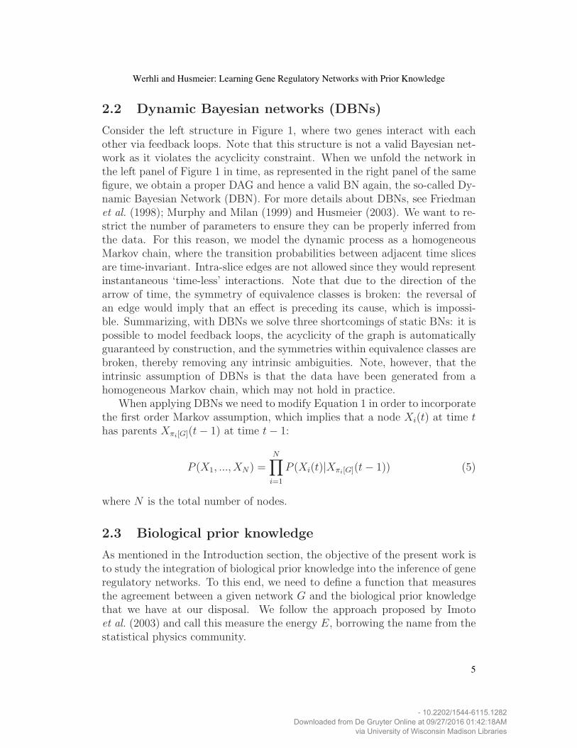
Figure 10: Raf signalling pathway. The graph shows the currently accepted Raf

signalling network, taken from Sachs et al. (2005). Nodes represent proteins, edges represent

interactions, and arrows indicate the direction of signal transduction.

our biological prior knowledge matrix. However, only 10 of the 25 studied genesare known to be TFs. For the remaining genes, no information about bindinglocations is available. The respective entries in the prior knowledge matrixwere thus set to Bij = 0.5, corresponding to the absence of prior information(see the discussion in Section 2.3).

Summarizing, we evaluated the performance of the proposed inferencescheme on two sets of gene expression data and two sets of TF binding lo-cation indications. An overview is given in Table 3.

4.3 Raf signalling pathway

Sachs et al. (2005) have applied intracellular multicolour flow cytometry exper-iments to quantitatively measure protein concentrations. Data were collectedafter a series of stimulatory cues and inhibitory interventions targeting spe-cific proteins in the Raf pathway. Raf is a critical signalling protein involvedin regulating cellular proliferation in human immune system cells. The dereg-ulation of the Raf pathway can lead to carcinogenesis, and this pathway hastherefore been extensively studied in the literature (e.g. Sachs et al. (2005);Dougherty et al. (2005)); see Figure 10 for a representation of the currently ac-cepted gold-standard network. In our experiments we used 5 data sets with 100measurements each, obtained by randomly sampling subsets from the originalobservational data of Sachs et al. (2005). Details about how we standardizedthe data can be found in Werhli et al. (2006).

We extracted biological prior knowledge from the Kyoto Encyclopedia ofGenes and Genomes (KEGG) pathways database (Kanehisa, 1997; Kanehisaand Goto, 2000; Kanehisa et al., 2006). KEGG pathways represent cur-

26


DOI: 10.2202/1544-6115.1282

- 10.2202/1544-6115.1282



Expression Data 1st source of Prior 2nd source of Prior1 Spellman Lee Harbison2 Tu Lee Harbison3 Spellman Lee MCMC Tu4 Tu Lee MCMC Spellman

Table 3: Yeast evaluation settings. This table summarizes the evaluation procedures

we used on the yeast data. The table shows the name of the first author of the data sets that

we used. Gene expression data: Spellman et al. (1998) and Tu et al. (2005). TF binding

location assays: Lee et al. (2002) and Harbison et al. (2004). The entries MCMC Spellman

and MCMC Tu indicate that the prior knowledge matrix was composed of the marginal

posterior probabilities of directed pairwise gene interactions (edges) obtained from running

MCMC simulations without prior knowledge on the respective expression data set.

rent knowledge of the molecular interaction and reaction networks related tometabolism, other cellular processes, and human diseases. As KEGG containsdifferent pathways for different diseases, molecular interactions and types ofmetabolism, it is possible to find the same pair of genes1 in more than onepathway. We therefore extracted all pathways from KEGG that contained atleast one pair of the 11 proteins/phospholipids included in the Raf pathway.We found 20 pathways that satisfied this condition. From these pathways, wecomputed the prior knowledge matrix, introduced in Section 2.3, as follows.Define by Mij the total number of times a pair of genes i and j appears in apathway, and by mij the number of times the genes are connected by a (di-rected) edge in the KEGG pathway. The elements Bij of the prior knowledgematrix are then defined by

Bij =mij

Mij(43)

If a pair of genes is not found in any of the KEGG pathways, we set therespective prior association to Bij = 0.5, implying that we have no informationabout this relationship.

1We use the term “gene” generically for all interacting nodes in the network. This mayinclude proteins encoded by the respective genes.

27


- 10.2202/1544-6115.1282



0 1 2 3 4 5 6x 105

0

0.2

0.4

0.6

0.8

1

1.2

1.4

1.6

1.8

MCMC Step

Data From Spellman et al

β Prior Leeβ Prior Harbison

(a)

0 1 2 3 4 5 6x 105

0

0.5

1

1.5

MCMC Step

Data From Tu et al

β Prior Leeβ Prior Harbison

(b)

0 0.5 1 1.5 20

0.2

0.4

0.6

0.8

1

1.2

1.4

1.6

PDF estimate − Spellman et al

β

(c)

0 0.5 1 1.5 20

0.2

0.4

0.6

0.8

1

1.2

1.4

1.6PDF estimate − Tu et al

β

(d)

Figure 11: Inferring hyperparameters associated with TF binding locations from

gene expression data of yeast. The top row (a,b) shows the hyperparameter trajectories

for two different sources of prior knowledge, sampled from the posterior distribution with the

MCMC scheme discussed in Section 2.4.2. The bottom row (c,d) shows the corresponding

marginal posterior probability densities, estimated from the MCMC trajectories with a

Parzen estimator, using a Gaussian kernel whose standard deviation was set automatically

by the MATLAB function ksdensity.m. The blue line represents the hyperparameter

associated with the TF binding locations of Lee et al. (2002). The red line shows the

hyperparameter associated with the TF binding locations of Harbison et al. (2004). The

two columns are related to different yeast microarray data. Left column: Spellman et al.

(1998). Right column: Tu et al. (2005). The two experiments correspond to the first two

rows of Table 3.

28


DOI: 10.2202/1544-6115.1282

- 10.2202/1544-6115.1282



how?

Lee et al 2002

Prior Probabilites from p−values

Harbison et al 2004

Figure 12: Transcription factor (TF) binding locations. The two Hinton diagrams

provide a qualitative display of the TF binding location assays of Lee et al. (2002) (left

panel) and Harbison et al. (2004) (right panel). The columns of the two matrices represent

10 known TFs. The rows represent 25 genes that are putatively regulated by the TFs. The

size of a white square represents the probability that a TF binds to the promoter of the

respective gene, with a larger square indicating a value closer to 1. These probabilities were

obtained by subjecting the p-values from the original immunopreciptation experiments of

Lee et al. (2002) and Harbison et al. (2004) to the transformation proposed by Bernard and

Hartemink (2005).

5 Results

5.1 Yeast cell cycle

For evaluating the performance of the proposed Bayesian inference schemeon the yeast cell cycle data, we followed Bernard and Hartemink (2005) withthe extension described in Section 4.2. We associated the edges of the BNwith conditional probabilities of the multinomial distribution family. In thiscase, the marginal likelihood P (D|G) of Equation 3 is given by the so-calledBDe score; see Heckerman (1999) for details. The chosen form of conditionalprobabilities requires a discretization of the data. Like Bernard and Hartemink(2005), we discretized the gene expression data into three levels using the infor-mation bottleneck algorithm, proposed by Hartemink (2001). We representedinformation about the cell cycle phase with a separate node, which was forcedto be a root node connected to all the nodes in the domain. In all our MCMC

29


- 10.2202/1544-6115.1282



0 1 2 3 4 5 6x 105

0

0.5

1

1.5

2

2.5

3

3.5

MCMC Step

Data From Spellman et al

β Prior Leeβ Prior Tu Results

(a)

0 1 2 3 4 5 6x 105

0

0.5

1

1.5

2

2.5

3

3.5

4

MCMC Step

Data From Tu et al

β Prior Leeβ Prior Spellman Results

(b)

0 1 2 3 40

0.2

0.4

0.6

0.8

1

1.2

1.4PDF estimate − Spellman et al

β

(c)

0 1 2 3 4 5 60

0.2

0.4

0.6

0.8

1

1.2

1.4PDF estimate − Tu et al

β

(d)

Figure 13: Inferring hyperparameters associated with priors of different nature.

The graphs are similar to those of Figure 11, but were obtained for different sources of prior

knowledge. The blue lines show the MCMC trace plots (top row) and estimated marginal

posterior probability distributions (bottom row) of the hyperparameter associated with the

TF binding locations from Lee et al. (2002). The red lines correspond to the hyperparameter

associated with prior knowledge obtained from an independent microarray experiment in the

way described in Section 5.1. The left column shows the results obtained from the experiment

corresponding to the third row of Table 3. The right column shows the results obtained from

the experiment corresponding to the fourth row of Table 3. For an explanation of the graphs,

see the caption of Figure 11.

30


DOI: 10.2202/1544-6115.1282

- 10.2202/1544-6115.1282



simulations, we combined gene expression data with two independent sourcesof prior knowledge, and sampled networks and hyperparameters from the con-ditional probability distribution according to the MCMC scheme described inSection 2.4.2.

Table 3 presents a summary of the simulation settings we used. In ourfirst application, corresponding to the first row of Table 3, the gene expressiondata were taken from Spellman et al. (1998). In our second application, corre-sponding to the second row of Table 3, the gene expression data came from Tuet al. (2005). In both applications, we used the same two independent sourcesof prior knowledge in the form of transcription factor (TF) binding locations(Lee et al., 2002; Harbison et al., 2004), as described in Section 4.2.

The MCMC trajectories of the hyperparameters associated with the twosources of biological prior knowledge are presented in Figure 11. The figurealso shows the estimated marginal posterior probability distributions of thetwo hyperparameters. These distributions, as well as the MCMC trace plots,do not appear to be very different, which suggests that the two priors aresimilar. A closer inspection of the results from the two TF binding assays,shown in Figure 12, reveals that the indications of putative TF binding loca-tions obtained independently by Lee et al. (2002) and Harbison et al. (2004)are, in fact, very similar. This finding confirms that the results obtained withthe proposed Bayesian inference scheme are consistent and in accordance withour expectation. From Figure 11 we also note that the sampled values ofthe hyperparameters are rather small, and that the estimated marginal poste-rior distributions – compared to those presented in the next section – are quiteclose to zero. This suggests that the prior information included is not in strongagreement with the data. There are two possible explanations for this effect.First, the TF activities might be controlled by post-translational modifica-tions, which implies that the gene expression data obtained from microarrayexperiments might not contain sufficient information for inferring regulatoryinteractions between TFs and the genes they regulate. Second, there might berelevant regulatory interactions between genes that do not belong to the set ofa priori known TFs, which are hence inherently undetectable by the bindingassays.

One might therefore assume that prior knowledge obtained on the basis ofa preceding microarray experiment might be more informative about a subse-quent second microarray experiment than TF binding locations. To test thisconjecture, we took one of the two gene expression data sets, assumed a uni-form prior on network structures (subject to the usual fan-in restriction), andsampled networks from the posterior distribution with MCMC. From this sam-ple, we obtained the marginal posterior probabilities of all edges, and used the

31


- 10.2202/1544-6115.1282



resulting matrix as a source of prior knowledge for the subsequent microarrayexperiment. We proceeded with the settings shown in the third and fourth rowof Table 3. First, we combined the results obtained from the gene expressiondata of Spellman et al. (1998) with the binding locations from Lee et al. (2002)and applied these two sources of prior knowledge to the gene expression datafrom Tu et al. (2005). Second, we combined the results obtained from the geneexpression data of Tu et al. (2005) with the binding locations from Lee et al.(2002) and applied these two sources of prior knowledge to the gene expressiondata from Spellman et al. (1998). The resulting hyperparameter trajectoriesare presented in Figure 13 together with their estimated probability densities.Compared with the previous results of Figure 11, there is now a much clearerseparation between the two distributions. The sampled values of the hyper-parameter associated with the second, independent source of microarray datasignificantly exceed those of the hyperparameter associated with the bindingdata. This suggests that prior knowledge that is more consistent with the datais given a stronger weight by the Bayesian inference scheme, in confirmationof our conjecture.

The critical question to ask next is: by how much does the accuracy ofnetwork reconstruction improve as a consequence of integrating prior knowl-edge into the inference scheme? Unfortunately, this evaluation cannot be donefor yeast owing to our lack of knowledge about the true gene regulatory in-teractions and the absence of a proper gold-standard network. To answer thisquestion, we therefore turn to a second application, for which more biologicalknowledge about the true regulatory processes exists.

5.2 Raf signalling pathway

5.2.1 Motivation

As described in Section 4.3, the Raf pathway has been extensively studied inthe literature. We therefore have a sufficiently reliable gold-standard networkfor evaluating the results of our inference procedure, as depicted in Figure 10.Additionally, recent work by Sachs et al. (2005) provides us with an abundanceof protein concentration data from cytometry experiments, and the authorshave also demonstrated the viability of learning the regulatory network fromthese data with Bayesian networks. However, the abundance of cytometry datasubstantially exceeds that of currently available gene expression data from mi-croarrays. We therefore pursued the approach taken in Werhli et al. (2006)and downsampled the data to a sample size representative of current microar-ray experiments (100 exemplars). As described in Section 4.3, the objective of

32


DOI: 10.2202/1544-6115.1282

- 10.2202/1544-6115.1282



interesting..

0 2 4 6 8 10x 104

0

0.5

1

1.5

2

2.5

3

3.5

4

4.5

MCMC Step

Real Data 1

β Prior KEGGβ Prior Random

(a)

0 1 2 3 4 50

0.1

0.2

0.3

0.4

0.5

0.6

0.7

0.8

0.9

β

PDF estimate Real data

β KEGGβ Random

(b)

Figure 14: Inferring hyperparameters from the cytometry data of the Raf path-

way. The left panel (a) shows the hyperparameter trajectories for two different sources of

prior knowledge, sampled from the posterior distribution with the MCMC scheme discussed

in Section 2.4.2. The right panel (b) shows the corresponding posterior probability densities,

estimated from the MCMC trajectories with a Parzen estimator, using a Gaussian kernel

whose standard deviation was set automatically by the MATLAB function ksdensity.m.

The blue lines refer to the hyperparameter associated with the prior knowledge extracted

from the KEGG pathways. The red lines refer to completely random and hence vacuous

prior knowledge. The data, on which the inference was based, consisted of 100 concentra-

tions of the 11 proteins in the Raf pathway, subsampled from the observational cytometry

data of Sachs et al. (2005).

33


- 10.2202/1544-6115.1282



UGE Obs DGE Obs0.5

0.55

0.6

0.65

0.7

0.75

0.8

0.85

0.9

0.95

1

AUC

Real Data − AUC

BNGGMBN−PriorOnlyPrior

(a)

UGE Obs DGE Obs0

2

4

6

8

10

12

14

16

18

20

TP C

ount

s, F

P=5

Real Data − TP

BNGGMBN−PriorOnlyPrior

(b)

Figure 15: Reconstruction of the Raf signalling pathway with different machine

learning methods. The figure evaluates the accuracy of inferring the Raf signalling path-

way from cytometry data and prior information from KEGG. Two evaluation criteria were

used. The left panel shows the results in terms of the area under the ROC curve (AUC

scores), while the right panel shows the number of predicted true positive (TP) edges for a

fixed number of 5 spurious edges. Each evaluation was carried out twice: with and with-

out taking the edge direction into consideration (UGE: undirected graph evaluation, DGE:

directed graph evaluation). Four machine learning methods were compared: Bayesian net-

works without prior knowledge (BNs), Graphical Gaussian Models without prior knowledge

(GGMs), Bayesian networks with prior knowledge from KEGG (BN-Prior), and prior knowl-

edge from KEGG only (Only Prior). In the latter case, the elements of the prior knowledge

matrix (introduced in Section 2.3) were computed from Equation 43. The histogram bars

represent the mean values obtained by averaging the results over five data sets of 100 protein

concentrations each, independently sampled from the observational cytometry data of Sachs

et al. (2005). The error bars show the respective standard deviations.

34


DOI: 10.2202/1544-6115.1282

- 10.2202/1544-6115.1282



0 20 40 60 80 1000.5

0.55

0.6

0.65

0.7

0.75

0.8

0.85

0.9

0.95

1DGE

AUC

β1

AUCβ1 MCMC trajectory

0 20 40 60 80 1000.5

0.55

0.6

0.65

0.7

0.75

0.8

0.85

0.9

0.95

1UGE

AUC

β1


0 5 10 15 20 25 300.5

0.55

0.6

0.65

0.7

0.75

0.8

0.85

0.9

0.95

1DGE

AUC

β1


0 5 10 15 20 25 300.5

0.55

0.6

0.65

0.7

0.75

0.8

0.85

0.9

0.95

1UGE

AUC

β1


Figure 16: Learning the hyperparameter associated with the prior knowledge

from KEGG. The horizontal axis represents the value of β1, the hyperparameter associated

with the prior knowledge from KEGG. The vertical axis represents the area under the ROC

curve (AUC). The blue line shows the mean AUC score for fixed values of β1, obtained by

sampling network structures from the posterior distribution with MCMC. The results were

averaged over five data sets of 100 protein concentrations each, independently sampled from

the observational cytometry data of Sachs et al. (2005). The error bars show the respective

standard deviations. The vertical red lines show trace plots of β1 obtained with the MCMC

scheme described in Section 2.4.2, where networks and hyperparameters are sampled from

the posterior distribution. Each evaluation was carried out twice, with and without taking

the edge direction into consideration. Right panel: undirected graph evaluation (UGE). Left

panel: directed graph evaluation (DGE). The bottom row presents a magnified view of the

left-most part of the graph.

35


- 10.2202/1544-6115.1282



our study is to assess the viability of the proposed Bayesian inference schemeand to estimate by how much the network reconstruction results improve asa consequence of combining the (down-sampled) cytometry data with priorknowledge from the KEGG pathway database. To this end, we compared theresults obtained with the methodology described in Section 2 with our earlierresults from Werhli et al. (2006), where we had evaluated the performance ofBayesian networks (BNs) and Graphical Gaussian models (GGMs) without theinclusion of prior knowledge. We applied GGMs as described in Schafer andStrimmer (2005). For comparability with Werhli et al. (2006), we used BNswith the family of linear Gaussian distributions, for which the marginal likeli-hood P (D|G) of Equation 3 is given by the so-called BGe score; see Geiger andHeckerman (1994) for details. Note that the cytometry data of Sachs et al.(2005) are not taken from a time course; hence, BNs were treated as staticrather than dynamic models.

5.2.2 Discriminating between different priors

We wanted to test whether the proposed Bayesian inference method can dis-criminate between different sources of prior knowledge and automatically as-sess their relative merits. To this end, we complemented the prior from theKEGG pathway database with a second prior, for which the entries in the priorknowledge matrix B were chosen completely at random. Hence, this secondsource of prior knowledge is vacuous and does not include any useful informa-tion for reconstructing the regulatory network. Figure 14 presents the MCMCtrajectories of the hyperparameters β1 and β2 together with their respectiveestimated probability distributions. The hyperparameter associated with theKEGG prior, β1, takes on substantially larger values than the hyperparameterassociated with the vacuous prior, β2. The estimated posterior distribution ofβ1 covers considerably larger values than the estimated posterior distributionof β2. This suggests that the proposed method successfully discriminates be-tween the two priors and effectively suppresses the influence of the vacuousprior. Note that the vacuous prior is not completely ‘switched off’, though,and that the sampled values of β2 are still substantially larger than zero. Thisseemingly counterintuitive behaviour is not a failure of the method, but ratheran intrinsic feature of the posterior probability landscape; see Figure 9 andthe discussion in Section 3.4.

36


DOI: 10.2202/1544-6115.1282

- 10.2202/1544-6115.1282



5.2.3 Reconstructing the regulatory network

While the true network is a directed graph, our reconstruction methods maylead to undirected, directed, or partially directed graphs2. To assess the perfor-mance of these methods, we applied two different criteria. The first approach,referred to as the undirected graph evaluation (UGE), discards the informationabout the edge directions altogether. To this end, the original and learnednetworks are replaced by their skeletons, where the skeleton is defined as thenetwork in which two nodes are connected by an undirected edge wheneverthey are connected by any type of edge. The second approach, referred toas the directed graph evaluation (DGE), compares the predicted network withthe original directed graph. A predicted undirected edge is interpreted as thesuperposition of two directed edges, pointing in opposite directions. The ap-plication of any of the machine learning methods considered in our study leadsto a matrix of scores associated with the edges in a network. For BNs sampledfrom the posterior distribution with MCMC, these scores are the marginalposterior probabilities of the edges. For GGMs, these are partial correlationcoefficients. Both scores define a ranking of the edges. This ranking definesa receiver operator characteristics (ROC) curve, where the relative number oftrue positive (TP) edges is plotted against the relative number of false positive(FP) edges. Ideally, we would like to evaluate the methods on the basis of thewhole ROC curves. Unfortunately, this approach would not allow us to con-cisely summarize the results. We therefore pursued two different approaches.The first approach is based on integrating the ROC curve so as to obtain thearea under the curve (AUC), with larger areas indicating, overall, a betterperformance. The second approach is based on the selection of an arbitrarythreshold on the edge scores, from which a specific network prediction is ob-tained. Following our earlier study (Werhli et al., 2006), we set the thresholdsuch that it led to a fixed count of 5 FPs. From the predicted network, wedetermined the number of correctly predicted (TP) edges, and took this scoreas our second figure of merit.

The results are shown in Figure 15. The proposed Bayesian inferencescheme clearly outperforms the methods that do not include the prior knowl-edge from the KEGG database (BNs and GGMs). It also clearly outperformsthe prediction that is solely based on the KEGG pathways alone without tak-ing account of the cytometry data. The improvement is significant for allfour evaluation criteria: AUC and TP scores for both directed (DGE) and

2GGMs are undirected graphs. While BNs are, in principle, directed graphs, partiallydirected graphs may result as a consequence of equivalence classes, which were briefly dis-cussed at the end of Section 2.1.

37


- 10.2202/1544-6115.1282



undirected (UGE) graph evaluations. This suggests that the network recon-struction accuracy can be substantially improved by systematically integratingexpression data with prior knowledge about pathways, as extracted from theliterature or databases like KEGG.

5.2.4 Learning the hyperparameters

While the study described in Section 5.2.2 suggests that the proposed Bayesianinference scheme succeeds in suppressing irrelevant prior knowledge, we werecurious to see whether the hyperparameter associated with the relevant prior(from KEGG) was optimally inferred. To this end, we chose a large set of fixedvalues for β1, while keeping the hyperparameter associated with the vacuousprior fixed at zero: β2 = 0. For each fixed value of β1, we sampled BNs from theposterior distribution with MCMC, and evaluated the network reconstructionaccuracy using the evaluation criteria described in Section 5.2.3. We com-pared these results with the proposed Bayesian inference scheme, where bothhyperparameters and networks are simultaneously sampled from the posteriordistribution with the MCMC scheme discussed in Section 2.4.2. The resultsare shown in Figure 16. The blue lines show plots of the various predictioncriteria obtained for fixed hyperparameters, plotted against β1. Plotted alongthe vertical direction, the red lines show MCMC trace plots for the sampledvalues of β1. These results suggest that the inferred values of β1 are close tothose that achieve the best network reconstruction accuracy. However, there isa small yet significant bias: the sampled values of β1 lie systematically belowthose that optimize the reconstruction performance. There are two possibleexplanations for this effect. First, recall that for static BNs as considered here,the partition function of Equation 15 is only approximated by Equation 21,which could lead to a systematic bias in the inference scheme. Second, it hasto be noted that the gold-standard Raf pathway reported in the literature isnot guaranteed to be the true biological regulatory network. Interestingly, arecent study (Dougherty et al., 2005) reports evidence for a negative feedbackinvolving Raf, which is not included in the assumed gold standard networktaken from Sachs et al. (2005). The existence of a hidden feedback loop act-ing on a putative feedforward path may lead to some systematic error in theedge directions, as static BNs are intrinsically restricted to the modelling of di-rected acyclic graphs. To shed further light on this issue, we therefore decidedto carry out an additional synthetic study.

38


DOI: 10.2202/1544-6115.1282

- 10.2202/1544-6115.1282



0 2 4 6 8 100.5

0.55

0.6

0.65

0.7

0.75

0.8

0.85

0.9

0.95

1DGE

AUC

β

(a)

0 2 4 6 8 100.5

0.55

0.6

0.65

0.7

0.75

0.8

0.85

0.9

0.95

1UGE

AUC

β

(b)

Figure 17: Learning the hyperparameter from synthetic data. The graphs corre-

spond to those of Figure 16, but were obtained from five independently generated synthetic

data sets. These data were generated from the gold-standard Raf signalling pathway re-

ported in Sachs et al. (2005), as described in Section 5.3. The prior knowledge was set to a

corrupted version of the gold-standard network, in which 6 (out of the 20) true edges had

been removed and replaced by wrong edges. For an explanation of the graphs and symbols,

see the caption of Figure 16.

39


- 10.2202/1544-6115.1282



5.3 Comparison with simulated data

We simulated synthetic data from the Raf signalling network, depicted in Fig-ure 10, as follows. Let Xi(t) denote a random variable that represents thehypothetical protein concentration of node i. We generated data from a linearGaussian distribution

Xi ∼ N(%

k

wikxk,σ2) (44)

where the sum extends over all parents of node i (that is, those nodes with anedge pointing to node i), and xk represents the value that node k takes on. Wetook the set of parents from the Raf signalling network, depicted in Figure 10,always initiating the process described by Equation 44 at the root, that is, nodepip3. We set the standard deviation to σ = 0.1, and the interaction strengthsto wik = 1. To mimic the situation described in the previous section, wegenerated 5 independent data sets with 100 samples each. As prior knowledge,we used a corrupted version of the true network, in which 6 (out of the 20)true edges had been removed and replaced by wrong edges. We then proceededwith the inference in the same way as described in Section 5.2. The resultsare shown in Figure 17, which corresponds to Figure 16 for the real cytometrydata. From a comparison of these two figures, we note that the small bias inthe inference of the hyperparameter has disappeared, and that values of thehyperparameter are sampled in the range where the reconstruction accuracy isoptimized. This suggests that the small bias observed in Figure 16 might notbe caused by the approximation of the partition function in Equation 21, butseems more likely to be a consequence of the other two effects discussed at theend of Section 5.2 (errors in the gold-standard network and putative feedbackloops).

6 Discussion

The work presented here is based on pioneering work by Imoto et al. (2003)on learning gene regulatory networks from expression data and biological priorknowledge, which has recently found a variety of applications (Tamada et al.,2003; Nariai et al., 2004; Tamada et al., 2005; Imoto et al., 2006). The idea isto express the available prior knowledge in terms of an energy function, fromwhich a prior distribution over network structures is obtained in the form ofa Gibbs distribution. The hyperparameter of this distribution, which corre-sponds to an inverse temperature in statistical physics, represents the weightassociated with the prior knowledge relative to the data. Our work comple-ments the work of Imoto et al. (2003) in various respects. We have extended

40


DOI: 10.2202/1544-6115.1282

- 10.2202/1544-6115.1282



the framework to multiple sources of prior knowledge; we have derived andtested an MCMC scheme for sampling networks and hyperparameters simul-taneously from the posterior distribution; we have elucidated intrinsic featuresof this scheme from an idealized network population amenable to a closed-formderivation of the posterior distribution; and we have assessed the viability ofthe proposed Bayesian inference approach on various synthetic and real-worlddata.

Our findings can be summarized as follows. When including two sourcesof prior knowledge of similar nature, the marginal posterior distributions ofthe associated hyperparameters are similar (Figure 11). When the two sourcesof prior knowledge are different, higher weight is assigned to the prior thatis more consistent with the data (Figure 13). When including an irrelevantprior with vacuous information, its influence will be automatically suppressed(Figure 14) in that the marginal posterior distribution of the correspondinghyperparameter is shifted towards zero. The irrelevant prior is not completelyswitched off, though. This would correspond to a delta distribution sittingat zero, which is never observed, not even for the worst-case scenario of priorknowledge that is in complete contradiction to the true network and the data(Figures 9c and d). To elucidate this unexpected behaviour, we carried outtwo types of analysis. In the first case, we considered an idealized popula-tion of network structures for which the prior distribution could be computedin closed form (Equation 41). In the second case, we considered networkscomposed of a small number of nodes (Figure 5), for which the partition func-tion of Equation 15, and hence the prior distribution over networks structures(Equation 14), could be numerically computed by exhaustive enumeration ofall possible structures. Both types of analysis reveal that the posterior dis-tribution over hyperparameters contains a flat plateau (Figure 9a-b), whichaccounts for our seemingly counter-intuitive observations.

We evaluated the accuracy of reconstructing the Raf protein signallingnetwork, which has been extensively studied in the literature. To this end,we combined protein concentrations from cytometry experiments with priorknowledge from the KEGG pathway database. The findings of our studyclearly demonstrate that the proposed Bayesian inference scheme outperformsvarious alternative methods that either take only the cytometry data or onlythe prior knowledge from KEGG into account (Figure 15). We inspected thevalues of the sampled hyperparameters. Encouragingly, we found that theirrange was close to the optimal value that maximizes the network reconstruc-tion accuracy (Figure 16). A small systematic deviation would be expectedowing to the approximation we have made for computing the partition func-tion of the prior (Equations 11 and 21). Interestingly, a comparison between

41


- 10.2202/1544-6115.1282



real and simulated cytometry data – Figure 16 versus Figure 17 – revealedthat the small bias only occurred in the former case. This suggests that otherconfounding factors, like errors in the gold-standard network and as yet unac-counted feedback loops, might have a stronger effect than the approximationmade for computing the partition function.

A certain shortcoming of the proposed method is the intrinsic asymmetrybetween prior knowledge and data, which manifests itself in the fact that thehyperparameters of the prior are inferred from the data. Ultimately, the priorknowledge is obtained from some data also; for instance, prior knowledge aboutTF binding sites is obtained from immunoprecipitation data. A challengingtopic for future research, hence, is to treat both prior and data on a moreequal footing, and to develop more systematic methods of postgenomic dataintegration.

References

Bernard,A. and Hartemink,A.J. (2005) Informative structure priors: jointlearning of dynamic regulatory networks from multiple types of data. InPacific Symposium on Biocomputing pp. 459–470 World Scientific, New Jer-sey.

Butte,A.S. and Kohane,I.S. (2003) Relevance networks: a first step towardfinding genetic regulatory networks within microarray data. In The Analysisof Gene Expression Data, (Parmigiani,G., Garett,E.S., Irizarry,R.A. andZeger,S.L., eds), pp. 428–446 Springer, New York.

Chickering,D.M. (1995) A transformational characterization of equivalentBayesian network structures. International Conference on Uncertainty inArtificial Intelligence (UAI), 11, 87–98.

Cowles,M.K. and Carlin,B.P. (1996) Markov chain Monte Carlo convergencediagnostics: a comparative review. Journal of the American Statistical As-sociation, 91, 883–904.

Dougherty,M.K., Muller,J., Ritt,D.A., Zhou,M., Zhou,X.Z., Copeland,T.D.,Conrads,T.P., Veenstra,T.D., Lu,K.P. and Morrison,D.K. (2005) Regulationof Raf-1 by direct feedback phosphorylation. Molecular Cell, 17, 215–224.

Friedman,N. and Koller,D. (2003) Being Bayesian about network structure.Machine Learning, 50, 95–126.

42


DOI: 10.2202/1544-6115.1282

- 10.2202/1544-6115.1282



Friedman,N., Linial,M., Nachman,I. and Pe’er,D. (2000) Using Bayesian net-works to analyze expression data. Journal of Computational Biology, 7,601–620.

Friedman,N., Murphy,K. and Russell,S. (1998) Learning the structure of dy-namic probabilistic networks. In Proceedings of the Fourteenth Conferenceon Uncertainty in Artificial Intelligence (UAI), (Cooper,G.F. and Moral,S.,eds), pp. 139–147 Morgan Kaufmann, San Francisco, CA.

Geiger,D. and Heckerman,D. (1994) Learning Gaussian networks. pp. 235–243Morgan Kaufmann, San Francisco, CA.

Giudici,P. and Castelo,R. (2003) Improving Markov chain Monte Carlo modelsearch for data mining. Machine Learning, 50, 127–158.

Harbison,C.T., Gordon,B.D., Lee,T.I., Rinaldi,N.J., Macisaac,K.D.,Danford,T.W., Hannett,N.M., Tagne,J.B., Reynolds,D.B., Yoo,J.,Jennings,E.G., Zeitlinger,J., Pokholok,D.K., Kellis,M., Rolfe,A.P.,Takusagawa,K.T., Lander,E.S., Gifford,D.K., Fraenkel,E. and Young,R.A.(2004) Transcriptional regulatory code of a eukaryotic genome. Nature,431 (7004), 99–104.

Hartemink,A.J. (2001). Principled computational methods for the validationand discovery of genetic regulatory networks. PhD thesis, MIT.

Hartemink,A.J., Gifford,D.K., Jaakkola,T.S. and Young,R.A. (2001) Usinggraphical models and genomic expression data to statistically validate mod-els of genetic regulatory networks. Pacific Symposium on Biocomputing, 6,422–433.

Hastings,W.K. (1970) Monte Carlo sampling methods using Markov chainsand their applications. Biometrika, 57, 97–109.

Heckerman,D. (1999) A tutorial on learning with Bayesian networks. In Learn-ing in Graphical Models, (Jordan,M.I., ed.), Adaptive Computation and Ma-chine Learning pp. 301–354 MIT Press, Cambridge, Massachusetts.

Heckerman,D., Geiger,D. and Chickering,D.M. (1995) Learning Bayesian net-works: the combination of knowledge and statistical data. Machine Learn-ing, 20, 245–274.

Husmeier,D. (2003) Sensitivity and specificity of inferring genetic regulatoryinteractions from microarray experiments with dynamic Bayesian networks.Bioinformatics, 19, 2271–2282.

43


- 10.2202/1544-6115.1282



Husmeier,D., Dybowski,R. and Roberts,S. (2005) Probabilistic Modeling inBioinformatics and Medical Informatics. Advanced Information and Knowl-edge Processing, Springer, New York.

Imoto,S., Higuchi,T., Goto,T., Kuhara,S. and Miyano,S. (2003) Combiningmicroarrays and biological knowledge for estimating gene networks viaBayesian networks. Proceedings IEEE Computer Society BioinformaticsConference, (CSB’03), 104–113.

Imoto,S., Higuchi,T., Goto,T. and Miyano,S. (2006) Error tolerant model forincorporating biological knowledge with expression data in estimating genenetworks. Statistical Methodology, 3 (1), 1–16.

Imoto,S., Kim,S., Goto,T., , Aburatani,S., Tashiro,K., Kuhara,S. andMiyano,S. (2003) Bayesian network and nonparametric heteroscedastic re-gression for nonlinear modeling of genetic network. Journal of Bioinformat-ics and Computational Biology, 1 (2), 231–252.

Kanehisa,M. (1997) A database for post-genome analysis. Trends Genet, 13,375–376.

Kanehisa,M. and Goto,S. (2000) KEGG: kyoto encyclopedia of genes andgenomes. Nucleic Acids Research, 28, 27–30.

Kanehisa,M., Goto,S., Hattori,M., Aoki-Kinoshita,K., Itoh,M., Kawashima,S.,Katayama,T., Araki,M. and Hirakawa,M. (2006) From genomics to chemicalgenomics: new developments in KEGG. Nucleic Acids Research, 34, D354–357.

Lee,T.I., Rinaldi,N.J., Robert,F., Odom,D.T., Bar-Joseph,Z., Gerber,G.K.,Hannett,N.M., Harbison,C.T., Thompson,C.M., Simon,I., Zeitlinger,J., Jen-nings,E.G., Murray,H.L., Gordon,D.B., Ren,B., Wyrick,J.J., Tagne,J.B.,Volkert,T.L., Fraenkel,E., Gifford,D.K. and Young,R.A. (2002) Transcrip-tional regulatory networks in Saccharomyces cerevisiae. . Science, 298(5594), 799–804.

Madigan,D. and York,J. (1995) Bayesian graphical models for discrete data.International Statistical Review, 63, 215–232.

Murphy,K. and Milan,S. (1999). Modelling gene expression data using dynamicBayesian networks. Technical report MIT artificial intelligence laboratory.

44


DOI: 10.2202/1544-6115.1282

- 10.2202/1544-6115.1282



Nariai,N., Kim,S., Imoto,S. and Miyano,S. (2004) Using protein-protein in-teractions for refining gene networks estimated from microarray data byBayesian networks. Pacific Symposium on Biocomputing, 9, 336–347.

Sachs,K., Perez,O., Pe’er,D., Lauffenburger,D.A. and Nolan,G.P. (2005)Causal protein-signaling networks derived from multiparameter single-celldata. Science, Vol 308, Issue 5721, 523-529 , 22 April 2005, 308 (5721),523–529.

Schafer,J. and Strimmer,K. (2005) A shrinkage approach to large-scale covari-ance matrix estimation and implications for functional genomics. StatisticalApplications in Genetics and Molecular Biology, 4. Article 32.

Spellman,P.T., Sherlock,G., Zhang,M.Q., Iyer,V.R., Anders,K., Eisen,M.B.,Brown,P.O., Botstein,D. and Futcher,B. (1998) Comprehensive identifica-tion of cell cycle-regulated genes of the yeast Saccharomyces cerevisiae bymicroarray hybridization. Mol Biol Cell, 9 (12), 3273–3297.

Tamada,Y., Bannai,H., Imoto,S., Katayama,T., Kanehisa,M. and Miyano,S.(2005) Utilizing evolutionary information and gene expression data for esti-mating gene networks with Bayesian network models. Journal of Bioinfor-matics and Computational Biology, 3 (6), 1295–1313.

Tamada,Y., Kim,S., Bannai,H., Imoto,S., Tashiro,K., Kuhara,S. andMiyano,S. (2003) Estimating gene networks from gene expression data bycombining Bayesian network model with promoter element detection. Bioin-formatics, 19, ii227–ii236.

Tu,B.P., Kudlicki,A., Rowicka,M. and Mcknight,S.L. (2005) Logic of the yeastmetabolic cycle: temporal compartmentalization of cellular processes. Sci-ence, 310 (5751), 1152–1158.

Werhli,A.V., Grzegorczyk,M. and Husmeier,D. (2006) Comparative evaluationof reverse engineering gene regulatory networks with relevance networks,graphical Gaussian models and Bayesian networks. Bioinformatics, 22(20), 2523–2531.

45


- 10.2202/1544-6115.1282



Statistical Applications in Genetics and Molecular...

Documents

Transcript of Statistical Applications in Genetics and Molecular...