State Estimation - univ-angers.fr

Ecole des JD MACS, 20 march 2009 1

State EstimationProbabilistic and Bounded-error approaches

Michel Kieffer

L2S - CNRS - SUPELEC - Univ Paris-Sud

[email protected]

Thursday 20 march 2009


1 Introduction

State estimation = generalization of parameter estimation.

State : set of quantity that characterizethe status of a system at a given time instant

(ex : position and speed of a ball).

State estimation=

Estimation of the state from measurements on the system.


State may evolve with time.

A priori information assumed available

– on the way the state evolves (dynamical equation)– on the way measurements are obtained on the system (measurement

equation)

Hypotheses made

– on the measurement noise,– state perturbations

will determine the choice for the tools used for state estimation.


2 Outline

– Discrete-time models– Assumptions– Probabilistic approach– Bounded-error approach

– Joint parameter and state estimation– Continuous-time models

– Assumptions– Bounded-error approach


3 Discrete-time models

Consider a system described by the discrete-time state equation

xk+1 = fk (xk,wk) , k = 0, 1, ..., (1)

where

– fk is a known function (possibly nonlinear and time-varying),– xk is the unknown state vector at time k,

– wk is some unknown state perturbation vector.

Measurements satisfy

y` = h`(x`,v`), ` = 1, ..., k, (2)

where

– h` is a known function (also possibly nonlinear and time-varying),– y` is the measurement vector at time `,– v` is some unknown measurement noise vector.


Depending on the nature of fk and h`

and

on the information assumed available about

the state perturbation and measurement noise

various types of state estimators are available.


4 Probabilistic approach

4.1 Assumptions

– wk, k ∈ N and vk, k ∈ N are i.i.d. sequences with known pdfs,– pdf of x0 based on no measurement is known.

Recursive computation ofp(xk|y1:k),

posterior pdf of xk based on k first measurements, possible at least inprinciple.

Optimal solution of the state estimation problem in a Bayesian sense.


4.2 Recursive algorithm

Alternates

– predictions, prior pdf p(xk|y1:k−1) computed via theChapman-Kolgomorov equation

p (xk|y1:k−1) =∫

p (xk|xk−1) p (xk−1|y1:k−1) dxk−1 (3)

→ involves the state equation

xk+1 = fk (xk,wk) , k = 0, 1, ...,


– corrections, new measurement yk taken into account to update the priorpdf into the posterior pdf p(xk|yk) via Bayes’ rule

p (xk|y1:k) =p (yk|xk) p (xk|y1:k−1)

p (yk|y1:k−1). (4)

→ involves the measurement equation

y` = h`(x`,v`), ` = 1, ..., k,

Usually, (3) and (4) very difficult to evaluate.

Approached solutions have to be derived.


4.3 Linear-Gaussian case

When

– fk and h` are linear,– the pdfs of

– x0,– the state perturbations– the measurement noiseare Gaussian with known mean and covariance matrix

Kalman filter is the optimal solution (Sorenson, 1985).


4.4 Non-linear-Gaussian case

When

– fk and h` are non-linear,– the pdfs of

– x0,– the state perturbations– the measurement noiseare Gaussian with known mean and covariance matrix


Extended Kalman filter (Gelb, 1974; Anderson and Moore, 1979)

→ linearization of the state and measurement equations

→ Gaussian approximation of all pdfs

⊕ Simple implementation

Actual state may get lost

Unscented Kalman filter (Julier and Uhlmann, 2004)

→ linearization of the state and measurement equations

→ approximation of the a priori pdf by some well-selected points

⊕ Simple implementation

⊕ Performs better than the Extended Kalman filter

Actual state may still get lost


Grid-based approach (Terwiesch and Agarwal, 1995; Burgard et al., 1996)

→ discretisation of the state-space using a fixed grid

⊕ Non-linear treatment

⊕ Integrals replaced by discrete sums more easily evaluated

Accuracy depends on the size of the grid

Complexity depends on the size of the grid and dimension of the state



Particle filtering approach (Gordon et al., 1993; Kitagawa, 1996; Pitt andShephard, 1999; Arulampalam et al., 2002)

→ approximation of the pdfs using clouds of points

⊕ Non-linear treatment

⊕ Integrals replaced by discrete sums more easily evaluated

Accuracy depends on the number of points

Rather complex management of the cloud



5 Bounded-error approach

5.1 Assumptions

Supports with known shapes are available for wk,vk and x0

– wk ∈ Wk, k ∈ N with known Wk, k ∈ N,– vk ∈ Vk, k ∈ N with known Vk, k ∈ N,– x0 ∈ X0, known.

Recursive computation of the set

Xk|1:k

of all state vectors that are compatible with

– the supports,– the measurements,– the models.


5.2 Recursive algorithm

Alternates

– predictions, set Xk|1:k assumed available, predicted set

Xk+1|1:k = fk(Xk|1:k, Vk

)(5)

→ involves the state equation.– corrections, new measurement yk+1 taken into account to update

Xk+1|1:k, corrected set

Xk+1|1:k+1 =x ∈ Xk+1|1:k : yk+1 ∈ hk+1(Xk+1|1:k, Wk+1)

. (6)

→ involves the measurement equation.


x1

x2

Xk k|1:

xk

y1

y2

Xk k+1|1: +1

Xk k+1|1:

y , Wk k+1 +1

hk+1

fkxk+1

When the hypotheses about the support are not violated⇓

Guaranteed state estimator(no compatible state vector may get lost)


5.3 Linear case

When

– fk and h` are linear,– state perturbation and measurement noise are

– additive,– with elliposidal support

Ellipsoidal approximation for Xk|1:k,see e.g., (Schweppe, 1968; Bertsekas and Rhodes, 1971; Schweppe, 1973)

and (Durieu et al., 1996; Durieu et al., 2001).

Weaker hypotheses on fk (perturbations) may be considered (Chernouskoand Rokityanskii, 2000; Calafiore and El Ghaoui, 2004; Polyak et al., 2004).

More details in the talk by S. Lesecq.


When

– fk and h` are linear,– state perturbation and measurement noise are

– additive,– with boxes as support

Parallelotopic approximation for Xk|1:k,see e.g., (Chisci et al., 1996).

Exact polytopic descriptionfor Xk|1:k,(Shamma and Tu, 1999).


5.4 Non-linear case

When fk and h` are non-linear, Xk|1:k may be

– non-convex– non-connected.

When

– h` is linear– State perturbation and measurement noise are

– additive,– with boxes as support

Parallelotopic approximation for Xk|1:k,(Shamma and Tu, 1997).


When

– fk and h` are non-linear,– state perturbation and measurement noise are

– with boxes or subpavings as support

Subpaving approximation for Xk|1:k,(Kieffer et al., 1998; Kieffer et al., 2002).


6 Joint parameter and state estimation

Assume that

xk+1 = fk (xk,pk,wk) , k = 0, 1, ..., (7)

andy` = h`(x`,pk,v`), ` = 1, ..., k, (8)

where

– fk and h` are known functions (possibly nonlinear and time-varying),– xk is the unknown state vector at time k,

– pk is some unknown parameter vector– wk and v` are some unknown state perturbation and measurement

vectors.


Joint estimation of xk and pk possibleby defining and extended state vector

xek =

(xT

k ,pTk

)T


Assumptions are required for the variations of pk with time

– constantp′

k = 0

and the following extended state equation may be defined

xek+1 =

fk (xek,wk)

0

k = 0, 1, ...,

– slowly varyingp′

k = wp`

and the following extended state equation may be defined

xek+1 =

fk (xek,wk)

wp`

k = 0, 1, ...,

– ...


7 Continuous-time models

Assume now that the dynamical equation is continuous-time

x′ =dxdt

= f (x (t) ,v (t) , t) , (9)

and that discrete-time measurements are available

y (tk) = h (x (tk) ,w (tk) , tk) . (10)

– Continuous-time extensions of the Kalman filter– Algebraic estimation techniques


7.1 Bounded-error context

When f and h are linear,

Ellipsoidal bounding still possible,see (Schweppe, 1968) and (Bertsekas and Rhodes, 1971).

When f and h are non-linear,

Box approximation,see the interval observer

(Alcaraz-Gonzalez et al., 1999; Gouze et al., 2000; Rapaport andGouze, 2003) and (Moisan et al., 2009)

(Raissi et al., 2004; Meslem et al., 2008)

Subpaving approximation(Jaulin, 2002; Kieffer and Walter, 2005; Kieffer and Walter, 2006).


Most of these techniques requirefor the prediction step,

guaranteed numerical integration of the state equation,see, e.g., (Moore, 1966; Berz and Makino, 1998; Nedialkov and

Jackson, 2001).

Correction step implemented as in the discrete-time case.


References

Alcaraz-Gonzalez, V., A. Genovesi, J. Harmand, A.V. Gonzalez, A. Rapaport and J.P.

Steyer (1999). Robust exponential nonlinear interval observer for a class of lumped

models useful in chemical and biochemical engineering. Application to a wastewater

treatment process. In : Proc. MISC’99 Workshop on Applications of Interval

Analysis to Systems and Control. Girona. pp. 225–235.

Anderson, B.D.O. and J.B. Moore (1979). Optimal Filtering. Prentice-Hall. Englewood

Cliffs.

Arulampalam, M., S. Maskell, N. Gordon and T. Clapp (2002). A tutorial on particle

filters for on-line non-linear/non-gaussian bayesian tracking. IEEE Trans. Signal

Processing 50(2), 174–188.

Bertsekas, D. P. and I. B. Rhodes (1971). Recursive state estimation for a

set-membership description of uncertainty. 16(2), 117–128.

Berz, M. and K. Makino (1998). Verified integration of ODEs and flows using differential

algebraic methods on high-order Taylor models. Reliable Computing 4(4), 361–369.

Burgard, W., D. Fox, D. Hennig and T. Schmidt (1996). Estimating the absolute

position of a mobile robot using position probability grids. In : Proc. Of the

Thirteenth National Conference on Artificial Intelligence. pp. 896–901.


Calafiore, G. and L. El Ghaoui (2004). Ellipsoidal bounds for uncertain linear equations

and dynamical systems. Automatica 40, 773–787.

Chernousko, F. L. and D. Y. Rokityanskii (2000). Ellipsoidal bounds on reachable sets of

dynamical systems with matrices subjected to uncertain perturbations. Journal of

Optimization Theory and Applications 104, 1–19.

Chisci, L., A. Garulli and G. Zappa (1996). Recursive state bounding by parallelotopes.

Automatica 32, 1049–1056.

Durieu, C., B. Polyak and E. Walter (1996). Trace versus determinant in ellipsoidal outer

bounding with application to state estimation. In : Proceedings of the 13th IFAC

World Congress. Vol. I. San Francisco, CA. pp. 43–48.

Durieu, C., E. Walter and B. Polyak (2001). Multi-input multi-output ellipsoidal state

bounding. Journal of Optimization Theory and Applications 111(2), 273–303.

Gelb, A. (1974). Applied Optimal Estimation. MIT Press. Cambridge, MA.

Gordon, N. J., D. J. Salmond and A. F. Smith (1993). Novel approach to

nonlinear/non-gaussian bayesian state estimation. IEE Procedings F

140(2), 107–113.

Gouze, J. L., A. Rapaport and Z. M. Hadj-Sadok (2000). Interval observers for uncertain

biological systems. Journal of Ecological Modelling (133), 45–56.

Jaulin, L. (2002). Nonlinear bounded-error state estimation of continuous-time systems.

Automatica 38, 1079–1082.


Julier, S. J. and J. K. Uhlmann (2004). Unscented filtering and nonlinear estimation.

Proceedings of the IEEE 92(3), 401–422.

Kieffer, M. and E. Walter (2005). Interval analysis for guaranteed nonlinear parameter

and state estimation. Mathematical and Computer Modelling of Dynamic Systems

11(2), 171–181.

Kieffer, M. and E. Walter (2006). Guaranteed nonlinear state estimation for

continuous–time dynamical models from discrete–time measurements. In : Preprints

of the 5th IFAC Symposium on Robust Control Design.

Kieffer, M., L. Jaulin and E. Walter (1998). Guaranteed recursive nonlinear state

estimation using interval analysis. In : Proceedings of the 37th IEEE Conference on

Decision and Control. Tampa, FL. pp. 3966–3971.

Kieffer, M., L. Jaulin and E. Walter (2002). Guaranteed recursive nonlinear state

bounding using interval analysis. International Journal of Adaptive Control and

Signal Processing 6(3), 193–218.

Kitagawa, G. (1996). Monte-Carlo filter and smoother for non-gaussian nonlinear state

space models. Journal of Computational and Graphical Statistics 5(1), 1–25.

Meslem, N., N. Ramdani and Y. Candau (2008). Guaranteed state bounding estimation

for uncertain non linear continuous systems using hybrid automata. In : Proc. IFAC

International Conference on Informatics in Control, Automation Robotics. Funchal,

Madeira.


Moisan, M., O. Bernard and J. L. Gouze (2009). Near optimal interval observers bundle

for uncertain bioreactors. Automatica 1, 291–295.

Moore, R. E. (1966). Interval Analysis. Prentice-Hall. Englewood Cliffs, NJ.

Nedialkov, N. S. and K. R. Jackson (2001). Methods for initial value problems for

ordinary differential equations. In : Perspectives on Enclosure Methods (U. Kulisch,

R. Lohner and A. Facius, Eds.). Springer-Verlag. Vienna. pp. 219–264.

Pitt, M. and N. Shephard (1999). Filtering via simulation : Auxiliary particle filters.

Journal of the American Statistical Association 94(446), 590–599.

Polyak, B.T., S.A. Nazin, C. Durieu and E. Walter (2004). Ellipsoidal parameter or state

estimation under model uncertainty. Automatica 40(7), 1171–1179.

Raissi, T, N. Ramdani and Y. Candau (2004). Set membership state and parameter

estimation for systems described by nonlinear differential equations. Automatica

40(10), 1771–1777.

Rapaport, A. and J.-L. Gouze (2003). Parallelotopic and practical observers for nonlinear

uncertain systems. Int. Journal of Control 76, 237–251.

Schweppe, F. C. (1968). Recursive state estimation : unknown but bounded errors and

system inputs. 13(1), 22–28.

Schweppe, F. C. (1973). Uncertain Dynamic Systems. Prentice-Hall. Englewood Cliffs,

NJ.


Shamma, J. S. and K.-Y. Tu (1997). Approximate set-valued observers for nonlinear

systems. 42(5), 648–658.

Shamma, J.S. and K.Y. Tu (1999). Set-valued observers and optimal disturbance

rejection. IEEE Transactions on Automatic Control 44(2), 253–264.

Sorenson, H. (1985). Kalman Filtering : Theory and Application. IEEE Press. New-York.

Terwiesch, P. and M. Agarwal (1995). A discretized non-linear state estimator for batch

processes.. Computers and Chemical Engineering 19, 155–169.


Bounded-error State Estimation

Interval approach

—

Michel Kieffer

March 18, 2009


Content

• Bounded-error state estimation using interval analysis

– Discrete-time

– Continuous-time


1 Discrete-time state estimation

1.1 Introduction

System

Model

u

ym

yDiscrete-time state equation :

xk+1 = fk (xk,wk,uk) .

Observation equation :

yk = hk (xk) + vk,

k = 1, . . . , N.

Problem :

Evaluate state xk using all available information.


1.2 Recursive nonlinear state estimation in a

bounded-error context

Hypotheses :

• at k = 0, x0 ∈ [x0] ,

• wk ∈ [wk,wk] , known for all past k,

• vk ∈ [vk,vk] , known for all past k,

• uk, known for all past k.

Problem :

Characterize set Xk|k of all xk compatible with hypotheses.


1.3 Idealized recursive state estimation

x1( )k

x2( )k

Xk k- -1| 1

xk-1


Idealized recursive state estimation

x1( )k

x2( )k

Xk k- -1| 1

xk-1

Xk k| 1-

fk

xk



x1( )k

x2( )k

Xk k- -1| 1

xk-1

y1( )k

y k2( )

Xk k| 1-

Yk

fk

xk



x1( )k

x2( )k

Xk k- -1| 1

xk-1

y1( )k

y k2( )

XO

kXk k| 1-

Yk

h

fk

xk



x1( )k

x2( )k

Xk k- -1| 1

xk-1

y1( )k

y k2( )

XO

kXk k| 1-

Yk

h

fk

xk

Xk k|

Prediction and correction steps alternate


1.4 Correction step

Set-inversion problem :

Find

XOk+1|k+1 = h−1

k+1 (yk+1 − [vk+1]) .

Solution provided by Sivia.

(similar to parameter estimation

problem with one measurement)


1.5 Prediction step

With discrete-time state equation

xk+1 = fk (xk,wk,uk) .

=⇒ ImageSp

[f ](.)

(a) initial subpaving (b) minced subpaving

(c) image boxes (d) image subpaving


1.6 Simple example: bouncing ball

Ball bouncing on floor, mass m, radius r

Statex = (x, x)T

Sampling period T = 0.1 s

No friction, rigid ball

Observation:

yk+1 = (1 0)xk + [−0.2, 0.2]

Prediction:

xk+1 = fk (xk)

obtained by exact discretisation.

x m

r

x

.

Nonlinear equations due to thebounce

x −→ −x


Actual initial state (unknown)

x0 = 5.2 m,0 m.s−1

Initial search box

[x0] = [3, 6] × [−3, 3]


k = 1, prediction


k = 1, correction


k = 1 . . . 20,

Takes 0.2 s on a AMD K6 at 1.5GHz


2 Continuous-time state estimation

2.1 Introduction

System

Model

u

ym

yContinuous-time state equation :

x′ =dx

dt= f (x,w,u) .

Observation equation :

y (ti) = h (x (ti)) + v (ti) ,

i = 1, . . . , N.

Problem :

Evaluate state x using all available information.


2.2 Recursive nonlinear state estimation in a

bounded-error context

Hypotheses :

• at t0, x (t0) ∈ [x0] ,

• w (t) ∈ [w (t) ,w (t)] , known for all past t,

• v (ti) ∈ [v (ti) ,v (ti)] , known for all past ti,

• u (t) , known for all past t.

Problem :

Characterize set X (t) of all x (t) compatible with hypotheses.


Previous results

• (Kieffer et al, CDC, 98) :

– discrete-time,

– set description with subpavings.

• (Gouze et al, J. Ecol. Mod., 00) :

– continuous-time,

– uncertain state equation,

– cooperative uncertain state equation bounded between cooperative systems,

– set description with boxes.

• (Jaulin, Automatica, 02) :


– no state perturbations,

– guaranteed numerical integration of non-punctual boxes,

– set description with subpavings.

• (Raissi et al., Automatica, 04)


– no state perturbations,

– improved guaranteed numerical integration of non-punctual boxes,

– set description with boxes.


Present context

• continuous-time,

• state perturbations,

• uncertain state equations bounded between point dynamical systems,

• set description with subpavings,


2.3 Idealized recursive state estimation

x1( )t

x2( )t

X( )ti

x( )ti



x1( )t

x2( )t

X( )ti

x( )ti

X+( )t

i+1

Á

x( )ti+1



x1( )t

x2( )t

X( )ti

x( )ti

y1( )ti+1

y t2 +1( )i

X+( )ti+1

Y( )ti+1

Á

x( )ti+1



x1( )t

x2( )t

X( )ti

x( )ti

y1( )ti+1

y t2 +1( )i

XO( )ti+1

X+( )ti+1

Y( )ti+1

h

Á

x( )ti+1



x1( )t

x2( )t

X( )ti

x( )ti

y1( )ti+1

y t2 +1( )i

X( )ti+1

XO( )ti+1

X+( )ti+1

Y( )ti+1

h

Á

x( )ti+1

Prediction and correction steps alternate


2.4 Correction step

Set-inversion problem :

Find

XO (ti) = h−1 (y (ti) − [v (ti)]) .

Solution provided by Sivia.

(similar to the discrete-time case)


2.5 Prediction step

©

Flow φ difficult to obtain in general.


Situation much simpler with discrete-time state equation

x (k + 1) = fk (xk,w,uk) .

=⇒ ImageSp

[f ](.)

(a) initial subpaving (b) minced subpaving

(c) image boxes (d) image subpaving


Guaranteed numerical integration of continuous-time state equation

x′ =dx

dt= f (x,w,u)

combined with ImageSp.

x1(0) x t1( )

x t2( )x2(0)

[x(0)]

When state equation/initial conditions not well known=⇒ no accurate box enclosures


Enclosure of state equation between two cooperative systems+

Guaranteed numerical integration of the cooperative systems

x1(0) x t1( )

x t2( )

x2(0)

[x(0)][x( )]t

Guaranteed version of Gouze’s interval observer

Accurate box enclosure


Enclosure of uncertain state equation between punctual dynamical systems+

Guaranteed numerical integration of the punctual systems+

ImageSp

x1(0) x t1( )

x t2( )x2(0)

[x( )]t

©

[x ] [p ]00 £

(x ,p*

00* )

p


2.6 Bounding the uncertain state equations

Using a reformulation of Muller’s theorems (Muller,1926).

Theorem 1 (Existence) Assume that the function f (x,p,w, t) is continuous on a

domain

T :

a 6 t 6 b

ω (t) 6 x 6 Ω (t)

p0

6 p 6 p0

w 6 w (t) 6 w

where ωi (t) and Ωi (t) , i = 1 . . . nx, are continuous on [a, b] and such that

1. ω (a) = x0 and Ω (a) = x0,

2. for i = 1 . . . nx,

D±ωi (t) 6 minTi(t)

fi (x,p,w, t) and D±Ωi (t) > maxTi(t)

fi (x,p,w, t) ,


where Ti (t) and Ti (t) are subsets of T defined by

Ti (t) :

t = t,

xi = ωi (t) ,

ωj (t) 6 xj 6 Ωj (t) , j 6= i,

p0

6 p 6 p0,

w 6 w (t) 6 w,

Ti (t) :

t = t,

xi = Ωi (t) ,

ωj (t) 6 xj 6 Ωj (t) , j 6= i,

p0

6 p 6 p0,

w 6 w (t) 6 w.

Then, for any x (0) ∈ [x0,x0], p ∈[

p0,p0

]

and w (t) a solution to the dynamical

system exists, which remains in

E :

a 6 t 6 b

ω (t) 6 x 6 Ω (t)

and equals x (0) at t = 0. ♦


Theorem 2 (Uniqueness) Moreover, if for any p ∈[

p0,p0

]

and w (t)

satisfying w 6 w (t) 6 w at any t ∈ [a, b] ,

f (x,p,w, t) is Lipschitz with respect to x over D,

then for any given x (0) , p and w (t), this solution is unique. ♦


Specific version when f (x,p,w, t) satisfies condition close to cooperativity.

Theorem 3 (cooperative) Assume that the function f (x,p,w, t) is continuous on a

domain T′ that is the same as T in Theorem 1 where ωi (t) and Ωi (t) are continuous

over [a, b] for i = 1 . . . nx and such that

1. ω (a) = x0 and Ω (a) = x0,

2. for i = 1 . . . nx,

D±ωi (t) 6 minT′

i(t)

fi (x,p,v, t) and D±Ωi (t) > maxT′

i(t)fi (x,p,v, t) ,

where T′i (t) and T

′i (t) are subsets of T defined by

T′i (t) = ω (t) ×

[

p0,p0

]

× [w,w] × t

T′i (t) = Ω (t) ×

[

p0,p0

]

× [w,w] × t .


Assume that, if for all t ∈ [a, b] and (x,y) ∈ [ω (t) ,Ω (t)]×2,

xi 6 yi, i = 1 . . . nx , i 6= j

⇓

fj (x,p,w, t) 6 fj (y,p,w, t) , j = 1 . . . nx

for all p ∈[

p0,p0

]

, w ∈ [w,w].

Then, for any x (0) ∈ [x0,x0], p ∈[

p0,p0

]

and w (t), the solution of the dynamical

system exists and remains in E and equals x (0) at t = 0.The uniqueness conditions are the same as in Theorem 1. ♦


Inclusion function for φ (t):

[φ] (t) = [ω (t) ,Ω (t)] .


2.7 Obtaining ω (t) and Ω (t)

• No cooperativity conditions.Build a system

x′ = g1(x,x,p

0,p0,w (t) ,w (t) , t), x (0) = x0,

x′ = g1(x,x,p0,p0,w (t) ,w (t) , t), x (0) = x0,

the solution(

ωT1 (t) ,ΩT

1 (t))T

of which satisfies the requirements ofTheorem 1.


• Cooperativity conditions.Build two systems

x′ = g2

(

x,p0,p0,w (t) ,w (t) , t

)

, x (0) = x0

x′ = g2

(

x,p0,p0,w (t) ,w (t) , t

)

, x (0) = x0

such that for all t ∈ [a, b], x ∈ D, p ∈[

p0,p0

]

and w ∈ [w (t) ,w (t)]

one has

g2

(

x,p0,p0,w (t) ,w (t) , t

)

6 f (x,p,w, t) (1)

and

g2

(

x,p0,p0,w (t) ,w (t) , t

)

> f (x,p,w, t) . (2)

Then the solutions ω2 (t) and Ω2 (t) of these two EDOs satisfy theconditions required by Theorem 3.


Example 1 When state equation can be written as

x′ = f0 (x,p,t) + w (t)

and when the components f0,i (x,p,t) , i = 1 . . . nx of f0 (x,p,t) are monotonic with

respect to x, p and v, except to xi, the functions g1, g1, g

2and g2 are easy to define.

For example, to build g1,i

, in the formal expression of f0,i (x,p,t) , replace

1. xi by xi,

2. for j 6= i, xj by xj if∂f0,i

∂xj6 0 and by xj if

∂f0,i

∂xj> 0 for all t ∈ [a, b] , x ∈ D and

p ∈ [p0,p0],

3. for k = 1 . . . np, pk by pk if∂f0,i

∂pk6 0 for all t ∈ [a, b] , x ∈ D and p ∈ [p

0,p0] and

by pk

if∂f0,i

∂pk> 0 for all t ∈ [a, b] , x ∈ D and p ∈ [p

0,p0].

At last, add wi (t) to the obtained expression. A similar construction of g1,i may be

performed, but with reversed monotonicity conditions.


2.8 Examples

1

k01

k21

k12

2

u

Figure 1: Two-compartment model

Parameters k12 and k21 constant.Parameter k01 depends nonlinearlyof the quantity of material presentin first compartment

k01 =p1

p2 + x1

.

Then

p = (p1, p2, k12, k21)T

.

Quantities of material in both compartments evolve according to

x′ =

−p4x1 −p1x1

1 + p2x1

+ p3x2 + u

p4x1 − p3x2

(3)


Initial state vector x0 = (1, 0) , assumed to be known.

For all t > 0, u (t) = 0.

No state perturbation is considered.

p is only assumed to belong to

[p0] = [0.9, 1.1] × [1.1, 1.3] × [0.45, 0.55] × [0.2, 0.3] .

Only content of second compartment is measured,

ym (tk) = x2 (tk) + v (tk) .

The evolution of the state of (3) is studied for t ∈ [0, 10].


2.8.1 Using only prediction

State equation is cooperative:

Lower dynamical system

x′ = g

c

(

x,p0,p0, t

)

, x (0) = x0 (4)

with

gc(·) =

−p4x1 −p1x1

1 + p2x1

+ p3x2 + u

p4x1 − p3x2

Upper dynamical system

x′ = gc

(

x,p0,p0, t

)

, x (0) = x0 (5)

with

gc (·) =

−p4x1 −

p1x1

1 + p2x1+ p3x2 + u

p4x1 − p3x2

With x0 = x0 = x0, Muller’s theorem is satisfied.


0 5 100

0.5

1

t

0 5 100

0.5

1

t

t t

x1

x2

Figure 2: Evolution of the state estimate using prediction only: direct nu-merical integration (dotted lines) and using cooperativity or its variant ofTheorem 3 (bold lines)


2.8.2 Taking measurements into account

Measurements are now available.

Data taken every 2 s, corrupted by an additive noise in [−0.05, 0.05].

[vk] = [−0.05, 0.05].

Table 1: Noisy data used for state estimation

tk 2 4 6 8 10

y (tk) 0.323 0.278 0.145 0.186 0.079


0 5 10 15 200

0.2

0.4

0.6

0.8

1

0 5 10 15 200

0.1

0.2

0.3

0.4

0.5

t t

x1

x2

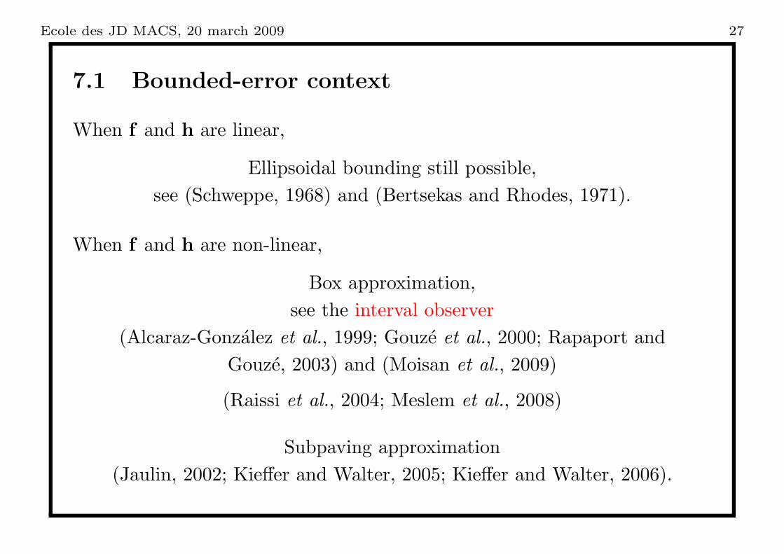
Figure 3: Comparison of two state estimation algorithm: SE-DNI (dottedlines) and SE-MY (bold line)

Computing times:

• 70 s for SE-DNI (direct numerical integration)

• 10 s for SE-MT (Muller’s theorem)


2.8.3 Joint parameter and state estimation

Now p4 added to the state vector x

xe =(

xT, p4

)T.

Assume p4 constant: extended dynamic

x′e =

−xe3xe1 −p1xe1

1 + p2xe1

+ p3xe2 + u

xe3xe1 − p3xe2

0

(6)

with xTe,0 =

(

xT0 , p

4

)

and xTe,0 =

(

xT0 , p4

)

.

New parameter vector

q = (p1, p2, p3)T∈ ([p1] , [p2] , [p3])

T.


Extended state equation not cooperative:

Coupled pair of dynamical systems

x′e = g

nc

(

xe,xe,q0,q0, t

)

, xe (0) = xe,0,

x′e = gnc

(

xe,xe,q0,q0, t

)

, xe (0) = xe,0,(7)

with

gnc

(·) =

−xe3xe1 −p1xe1

1 + p2xe1

+ p3xe2 + u

xe3xe1 − p3xe2

0

and

gnc (·) =

−xe3xe1 −p1xe1

1 + p2xe1

+ p3xe2 + u

xe3xe1 − p3xe2

0

have solutions satisfying Theorem 1.


Data simulated on the same nominal system as before.

Noise corrupting the measurement in [−0.005, 0.005].

All parameters (except p4) assumed perfectly known.

At t = 0, p4 is only known to belong to [0.1, 0.5].

0 5 10 15 200

0.2

0.4

0.6

0.8

1

0 5 10 15 200

0.1

0.2

0.3

0.4

0 5 10 15 200

0.1

0.2

0.3

0.4

0.5

t t

t

xe1

xe2

xe3

Takes 40 s on an Athlon at 1.5 GHz.


2.9 Summary of results

1. Recursive state estimation algorithm for continuous-time systems

2. Enclosure of uncertain dynamical system between two point dynamicalsystems

3. Uncertain parameters or state equations can be considered.

4. Computational complexity compatible with systems of large time constantssuch as those encountered in biology, pharmacokinetics...


Distributed parameter and state estimation

in a network of sensors

Michel Kieffer

L2S - CNRS - SUPELEC - Univ Paris-Sud

March 18, 2009


Wireless sensor networks?

Spatially distributed autonomous devices using sensors connected via awireless network.

Sensors may be for

• pressure

• temperature

• sound

• vibration

• motion

• ...

Initially developped for military applications (battlefield surveillance)Now, many civilian applications

(environment monitoring, home automation, traffic control)

[KM04, Hae06]


Applications suggest of many research topics

• protocols for communication between sensors,

• position and localization,

• data compression and aggregation,

• security,

• ...

Constraints on WSN

• limited computing capabilities,

• limited communication capacity,

• power consumption restricted.


Example: WSN for source tracking

Applications

• mobile phone localization andtracking

• computer localization in anad-hoc network

• co-localisation in a team ofrobots

• speaker localization

• . . .

Source (o) and sensors (x)


Usual methods based on

• Time of arrival→ requires good clock synchronization

• Time difference of arrival→ sensors cannot work independently

• Angle of arrival→ difficult to obtain

• Readings of signal strengh (RSS)→ cheap, but not accurate


Two localization approaches using RSS

• Centralized→ all measurements are processed by a unique processing unit

• Distributed→ measurements are processed by each sensor

Centralized Distributed

Context :

• bounded-error distributed estimation

• interval analysis


Distributed state estimation

Consider a system described by a discrete-time model

xk = fk (xk−1,wk,uk) , (1)

where

• xk state of model at time instant k (sampling period T )

• wk state perturbations, assumed bounded in known [w],

• uk input vector, assumed known.

At k = 0, x0 assumed to belong to a set X0, known.


Assume that each sensor ` = 1 . . . L of a WSN has access to a measurement

y`k = g`

k

(xk,v`

k

), (2)

where

• y`k noisy measurement,

• v`k measurement noise, assumed bounded in known [v],

(1) and (2) are the dynamic and observation equations of the model

Usual measurement equations

g`k

(xk,v`

k

)= h`

k (xk) + v`k

g`k

(xk, v`

k

)= h`

k (xk) .v`k


Back to centralized discrete-time state estimation

When all measurements at time k are available at central processing unit,one gets

xk = fk (xk−1,wk,uk) ,

yk = gk (xk,vk) ,

with yTk =

((y1

k

)T, . . . ,

(yL

k

)T) and vTk =

((v1

k

)T, . . . ,

(vL

k

)T).Standard (centralized) state estimation problem.


Information available at time k

Ik =

X0, [wj ]kj=1 , [vj ]k

j=1 , [yj ]kj=1

.

Centralized bounded-error state estimate at time k:

set Xk|k of all values of xk that are consistent with (1), (2) and Ik.

Idealized algorithm

1. Prediction step

Xk|k−1 =fk (x,w,uk) | x ∈ Xk−1|k−1, w ∈ [w]

2. Correction step

Xk|k =x ∈ Xk|k−1 | yk = gk (x,v) , v ∈ [v]×L

.


Distributed state estimation

Ideally, any sensor ` of the WSN should provide

X`k|k = Xk|k.

Previous work on this topic

• distributed Kalman filtering [Spe79]→ linear models, gaussian noise, instantaneous communications

• application to distributed estimation in power systems [LC05]

• distributed estimation in WSN [RGR06]


Hypotheses

Sensor network is entirely connected (necessary condition to haveX`

k|k = Xk|k)

At time k

• each sensor processes own measurement y`k.

Between time k and k + 1

• each sensor ` broadcasts estimates X`,rk|k

• each sensor ` receives and processes Xs,1k|k, s ∈ C (`) where C (`) set of

indices of sensors connected to `

Process may be repeated (several roundtrips ).

Before k + 1,

• each sensor ` builds an estimate X`k|k.


One may easily prove thatXk|k ⊂ X`

k|k.

Non-trivial conditions to have

Xk|k = X`k|k

are more difficult to obtain. Involve

• network connectivity

• largest distance (in links) between sensors

• ...

Problem studied in [Yok01, BFV+05].


Practical algorithm

Implementation issues:

• Boxes or subpavings used to represent sets,

• Basic interval evaluation or ImageSp [KJW02] for prediction step,

• Interval constraint propagation or Sivia [JW93] for correction step


Application: Static source localization

Known sensor locations

r` ∈ R2, ` = 1 . . . L

Unknown source location

θ = (θ1, θ2) ∈ R2

40 45 50 55 6040

42

44

46

48

50

52

54

56

58

60

Source (o) and sensors (x)


Mean power P (d`) (in dBm) received by `-th sensor described byOkumura-Hata model

P dB (d`) = P0 − 10np logd`

d0, (3)

where

• np is the path-loss exponent (unknown, but constant)

• d` = |r` − θ|.

Received power assumed to remain within some known bounds (here)

PdB (d) ∈[P0 − 10np log

d

d0− e, P0 − 10np log

d

d0+ e

], (4)

where e is assumed known→ bounded-error approach.


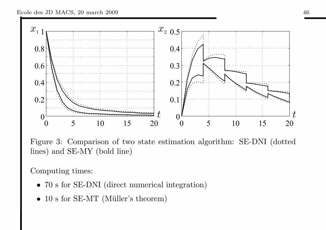
Bounded-error parameter estimation

RSS by sensor ` = 1 . . . L

y` = h` (θ, A, np) v`

with

h` (θ, A, np) =A

|r` − θ|np , A = 10P0/10dnp0 , (5)

andv` ∈ [v] =

[10−e/10, 10e/10

].

Constant state vector to be estimated

x = (A,np, θ1, θ2)


Distributed approach: interval constraint propagation

At sensor `,

• y` ∈ [y`], measured

• θ ∈ [θ], obtained from neighbors

• A ∈ [A], obtained from neighbors

• np ∈ [np], obtained from neighbors.

Variables must satisfy constraint provided by RSS model

y` −A

|r` − θ|np = 0. (6)

Interval constraint propagation :reduce the domains for the variables using the constraints


Contracted domains may be written as

[y′`] = [y`] ∩[A]

|r` − [θ]|[np],

[A′] = [A] ∩ [y′`] |r` − [θ]|[np],[

n′p]

= [np] ∩ (log ([A′])− log ([y′`])) / log (|r` − [θ]|) ,[θ′1]

= [θ1] ∩(

r`,1 ±√

([A′] / [y′`])2/[n′

p] − (r`,2 − [θ2])2

),

[θ′2]

= [θ2] ∩(

r`,2 ±√

([A′] / [y′`])2/[n′

p] − (r`,1 − [θ1])2

).

Contracted domains still contains all solutions


Results

Networks of L = 2000 sensors randomly distributed

Field of 100 m×100 m.

Source

• placed at θ∗ = (50 m, 50 m)

• P0 = 20 dBm

• d0 = 1 m

• np = 2 (constant over the field)

Measurement noise such that e = 4 dBm.


Example of measurements

Sensor 68 741 954 · · ·

Measurement [9.303, 58.698] [17.856, 112.664] [18.644, 117.640] · · ·

Initial search box (Unknown source amplitude)

[θ]× [A]× [np] = [0, 100]× [0, 100]× [50, 250]× [2, 4]

Initial search box (Known source amplitude)

[θ]× [A]× [np] = [0, 100]× [0, 100]× [100, 100]× [2, 4]


40 45 50 55 6040

42

44

46

48

50

52

54

56

58

60

40 45 50 55 6040

42

44

46

48

50

52

54

56

58

60

Unknown source amplitude Known source amplitude

µ1

µ2

µ1

µ2

Projection of the solution on the (θ1, θ2)-plane



µ1 µ1

µ2µ2

Zoom on the solution


Results – continued

0 1 2 30

5

10

15

20

25

Closest point approach

0 1 2 30

20

40

60

80

Distributed

0 1 2 30

20

40

60

80

Centralized

0 1 2 30

5

10

15

20

25

Closest point approach

0 1 2 30

10

20

30

40

50

Distributed

0 1 2 30

10

20

30

40

50

Centralized


Histograms of estimation error for θ (100 realizations of sensor field)


Application: Source tracking

Assume now that the source is moving. A and np assumed to be known.

New state vector

xk = (θ1,k, θ2,k, φ1,k, φ2,k, θ1,k−1, θ2,k−1, φ1,k−1, φ2,k−1)T

This long state vector allows to estimate(φ1,k, φ2,k

).


State vector evolves according to

θ1,k

θ2,k

φ1,k

φ2,k

θ1,k−1

θ2,k−1

φ1,k−1

φ2,k−1

=

I4 04

I4 04

θ1,k−1

θ2,k−1

φ1,k−1

φ2,k−1

θ1,k−2

θ2,k−2

φ1,k−2

φ2,k−2

+ T.

φ1,k−1

φ2,k−1

w1

w2

0

0

0

0

,

with w1 ∈ [w] and w2 ∈ [w].


Contracted domains

[y′`,k

]= [y`,k] ∩ A

|r` − [θk]|[np],

[θ′1,k

]= [θ1,k] ∩

(r`,1 ±

√(A/[y′`,k

])2/np

− (r`,2 − [θ2,k])2)

,

[θ′2,k

]= [θ2,k] ∩

(r`,2 ±

√(A/[y′`,k

])2/np

− (r`,1 − [θ1,k])2)

.

[φ′1,k

]=[φ1,k

]∩

([θ′1,k

]−[θ′1,k

]T

+ T [w]

)[φ′2,k

]=[φ2,k

]∩

([θ′2,k

]−[θ′2,k

]T

+ T [w]

)


Results

Field of 50 m×50 m (origin at center)

Networks of L = 25 sensors (communication range of 15 m)

Source

• placed at θ∗ = (5 m, 5 m)

• P0 = 20 dBm

• d0 = 1 m

• np = 2 (constant over the field)

• [w] = [−0.5, 0.5] m.s−2

• T = 0.5 s

Measurement noise such that e = 4 dBm.


-25 -20 -15 -10 -5 0 5 10 15 20 25

-25

-20

-15

-10

-5

0

5

10

15

20

25

Evolution of the source in the WSN


Localization error and width of the box [θ1,k]× [θ2,k]

First iteration

Convergence quite fast


Localization error and width of the box [θ1,k]× [θ2,k]

Third iteration

Convergence quite fast


Conclusions

• Distributed source localization

• Estimation in a bounded-error context→ guaranteed results (provided hypotheses satisfied)

Further work

• Large space for improvements (compute subpavings and send boxes)

• Robustness to outliers in a distributed context

• Sensor colocalisation (team of robots)

• ...

Work partly supported by NoE NEWCOM++


Overview of the components of the Embedded Sensor Board (ESB)from the FU-Berlin (picture from [Hae06]).


References

[BFV+05] R. Bejar, C. Fernandez, M. Valls, C. Domshlak, C. Gomes,B. Selman, and B. Krishnamachari. Sensor networks anddistributed CSP: Communication, computation and complexity.Artificial Intelligence Journal, 161(1-2):117–148, 2005.

[Hae06] T. Haenselmann. Sensornetworks. GFDL Wireless SensorNetwork textbook. 2006.http://www.informatik.uni-mannheim.de/haensel/sn book.

[JW93] L. Jaulin and E. Walter. Set inversion via interval analysis fornonlinear bounded-error estimation. Automatica,29(4):1053–1064, 1993.

[KJW02] M. Kieffer, L. Jaulin, and E. Walter. Guaranteed recursivenonlinear state bounding using interval analysis. InternationalJournal of Adaptive Control and Signal Processing,


6(3):193–218, 2002.

[KM04] R. Kay and F. Mattern. The design space of wireless sensornetworks. IEEE Wireless Communications, 11(6):54–61, 2004.

[LC05] S.-S. Lin and Huay Chang. An efficient algorithm for solvingdistributed state estimator and laboratory implementation. InICPADS ’05: Proceedings of the 11th International Conferenceon Parallel and Distributed Systems (ICPADS’05), pages689–694, Washington, DC, USA, 2005. IEEE Computer Society.

[RGR06] A. Ribeiro, G. B. Giannakis, and S. I. Roumeliotis. SOI-KF:Distributed Kalman filtering with low-cost communicationsusing the sign of innovations. IEEE Trans. Signal Processing,54(12):4782–4795, December 2006.

[Spe79] J. Speyer. Computation and transmission requirements for adecentralized linear-quadratic-gaussian control problem. IEEETrans. Automatic Control, 24(2):266–269, April 1979.


[Yok01] M. Yokoo. Distributed Constraint Satisfaction: Foundations ofCooperation in Multi-Agent Systems. Springer-Verlag, Berlin,2001.

State Estimation - univ-angers.fr

Documents

Transcript of State Estimation - univ-angers.fr