Stata Tutorial IT2010 - DSEdse.univr.it/it/documents/it5/stata_tutorial.pdf · ......

C.I.D.E.

Introduction -1- Environment -2.a- System Syntax -2.b- Statistical Syntax -3- Output

Stata Tutorial—

IT2010

Francesco Andreoli – Andrea Bonfatti

Università di Verona

January 11-15, 2010Alba di Canazei

Francesco Andreoli - Andrea Bonfatti (Università di Verona)Stata Tutorial January 11-15, 2010 1 / 59

C.I.D.E.


AcknowledgementsDepartment of Economics (DSE) - Università di Verona

- - -Nicola Tommasi (CIDE and Università di Verona) provided valuable

support with related documents and an early version of thispresentation.


C.I.D.E.


Organization of the Directory../stata_tutorial

||--> /read_me_first.txt||--> /tutorial.pdf * You are here! *||--> /data_files| || |--> /smallPSELL.dta| |--> /smallPSELL.csv| |--> /smallPSELL.txt| |--> /smallPSELL2.dta| |--> /smallPSELL2.csv| |--> /smallPSELL2.txt| |--> /estimates.txt||--> /do_files

||--> /do_first.do|--> /do_first.log|--> /model.txt|--> /model.gph


C.I.D.E.


Motivation

This tutorial addresses to a beginner level or early trained audiencewhich needs notions as well as operational hints to get started withStata software. This handout is meant to provide a support for a twohours tutorial, and it can be considered complementary to othermore exhaustive and rigorous sources.

You are invited to take a look at the Official Stata website,http://www.stata.com/bookstore/documentation.html, where youcan find all published documents. The “Getting Started with Stata”manual is an introductory (although very complete) users manual.


C.I.D.E.


Motivation

Additional material can be found in official websites:

http://www.stata.com/bookstore/pdf/gsw_samplesession.pdfhttp://www.stata.com/bookstore/pdf/r_intro.pdf (commands)http://www.stata.com/bookstore/pdf/g_graph_intro.pdf (graphs)http://www.stata.com/bookstore/pdf/d_merge.pdf (merge)

and unofficial ones:

http://www.ats.ucla.edu/stat/stata/http://www.nyu.edu/its/statistics/Docs/Intro_stata5.pdfhttp://www.eui.eu/Personal/Researchers/decio/PS/Stata.pdfhttp://leuven.economists.nl/stata/stataintro.pdf


C.I.D.E.


Organization of the Tutorial

The tutorial focuses on Stata for Windows package, SE version, actually at the11th release (the same procedure holds for older releases and other versions).Firstly, the tutorial will exploit the general settings of the environment wherethe data are stored, managed and analyzed. Here we will look closely on howorganize data into folders and how to work with a hierarchy of folders, in orderto make the research work intelligible by all audienced. Order is necessary towork scientifically, i.e. to be able to replicate an experiment starting from theobserved phenomena, preserving the measurability. Moreover, order is aprerequisite for understanding and interpretability of results.

On a second stage, attention will be paid to programming and coding and thegeneral setting of the program will be introduced: windows, interface, .do.dta .log .ado extensions, input/output of data files, basic syntax (datamanagement, statistics, regression, principles of graphs).


C.I.D.E.


Organization of the Tutorial

The concluding stage of the tutorial aims at showing how Stata works inpractice, by applying the program (.do file) to a small subsample (50 times 8)from the PSELL (Panel Socio-économique “Liewen zu Lëtzebuerg”) database(.dta file). Finally, Stata output will be described and analyzed (.log file).

The handout structure follows the tutorial sectioning. As a general purpose,you will be given with the means to autonomously search and apply newsyntax already stored in Stata memory (.ado files) or downloadable from theweb sites of Stata Journal, Stata Technical Bullettin or from Repec Library.The use of any particular syntax, as the one treated in classes to performincome distribution analysis, depends on your research scopes. For moreadvanced users, Stata offers the possibility to code new functions according toprogram language standards.


C.I.D.E.


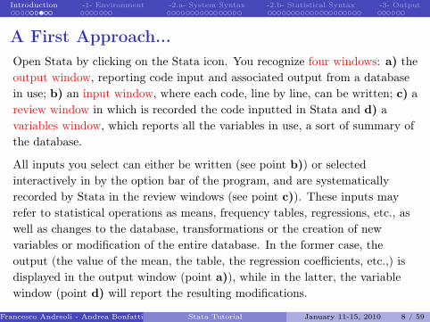
A First Approach...Open Stata by clicking on the Stata icon. You recognize four windows: a) theoutput window, reporting code input and associated output from a databasein use; b) an input window, where each code, line by line, can be written; c) areview window in which is recorded the code inputted in Stata and d) avariables window, which reports all the variables in use, a sort of summary ofthe database.

All inputs you select can either be written (see point b)) or selectedinteractively in by the option bar of the program, and are systematicallyrecorded by Stata in the review windows (see point c)). These inputs mayrefer to statistical operations as means, frequency tables, regressions, etc., aswell as changes to the database, transformations or the creation of newvariables or modification of the entire database. In the former case, theoutput (the value of the mean, the table, the regression coefficients, etc.,) isdisplayed in the output window (point a)), while in the latter, the variablewindow (point d) will report the resulting modifications.


C.I.D.E.


A First Approach...

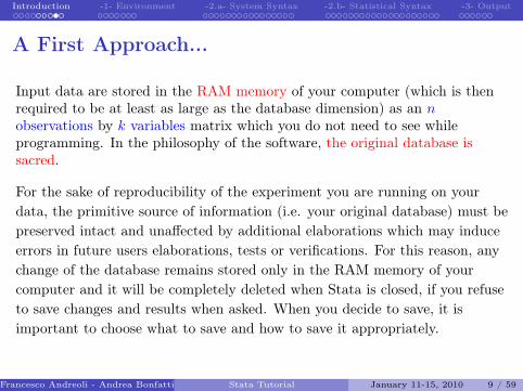
Input data are stored in the RAM memory of your computer (which is thenrequired to be at least as large as the database dimension) as an nobservations by k variables matrix which you do not need to see whileprogramming. In the philosophy of the software, the original database issacred.

For the sake of reproducibility of the experiment you are running on yourdata, the primitive source of information (i.e. your original database) must bepreserved intact and unaffected by additional elaborations which may induceerrors in future users elaborations, tests or verifications. For this reason, anychange of the database remains stored only in the RAM memory of yourcomputer and it will be completely deleted when Stata is closed, if you refuseto save changes and results when asked. When you decide to save, it isimportant to choose what to save and how to save it appropriately.


C.I.D.E.


A First Approach...Three fundamental steps:

1 If the original database has been modified, a new database must becreated containing all new variables and transformations performed. Inthis way, the original database will be preserved as an independentobject from the new one, but any information about how to go from onedatabase to the other will be lost. If the original database is notmodified, there is no need to save it and you will not be even asked to doso. Stata opens and saves databases in the .dta extention.

2 Output results can be saved in a log-on file, reporting a list of yourresults in a .txt extension. From this file you can copy tables orcoefficient results to be used in you research report. In Stata jargon, thisis a log-file.

3 Inputs as well can be saved, reporting the full list of commands appearingin the review window on a .txt document. This list can be used byother readers to understand how the new database and the output savedin the log file were obtained. In Stata jargon, this is a do-file.


C.I.D.E.


Setting the EnvironmentThe scope of this section is to show how to correctly manage your input,commands and output files for the sake of reproducibility and intelligibility ofyour work. The first object you need to manage is the initial source of data.The original database is your primitive source of information, therefore itmust be preserved on its original status. Data can be read, and you can workwith them, but never modify or delete them because they represent theprimitive source of information. Stata programming must be created to workwith relative paths which can be used in any file system.

A path, the general form of a filename or of a directory name, specifies aunique location in a file system. A relative path is a path relative to theworking directory of the user or application (eg:../stata_tutorial/do_files/do_first.do) which does not need to dependon the full path root usually system specific(C://Francesco_Andrea/IT2010/stata_tutorial/do_files/do_first.do).


C.I.D.E.


Setting the EnvironmentGolden rules in Stata

Generate a directory projects in which to put in all your currentprojects;Inside a specific project, take documents, data, programs asdistinct elements;In the data directory put your database. It is your original object;In the programs directory put your coding and the statisticalresults;Statistical results can be used either directly in a paper (graphs,tables,...) or by other softwares (derived databases, parametersestimates,...);Use simple names for files. File log in accordance withprogramming file. Be sequential. Use comments and alwaysdescribe what you are doing.


C.I.D.E.


Files Extentions in Stata

.dta data files, also in .csv or .txt.do program file containing coding, the starting point

.log; .smcl output logging files, results storing.ado files used by programmers, advanced code

.mata file extention in Mata environment.hlp; .sthlp help files.scheme; .style; .gph extension for graph attributes and to save

graphs


C.I.D.E.


Commands

All Stata commands are contructed following a precise syntaxstructure, allowing you to recognize always what is the commandemployed, the variables in use and the options, even for previouslyunseen objects. In this way, you can search for command help files.

The general syntax of a command:

command[varlist

][=exp

][if

][in

][weight

][, options

]mandatory coding between bracketsoptional coding between

[ ]commands in { } are parameters whose value must be specifiedunderlined letters are abbreviations for commandsparts in ’,’ are the commands options


C.I.D.E.


HelpThe general syntax for help, search, find

help[command_or_topic_name

][, options

]search word

[word ...

][, search_options

]findit word

[word ...

]Help is the most important command in Stata. It provides the fulldictionary and help of the commandlist specified.Use help! You cannot (and you must not) recall all commandsoptions and possible applications.Each help file, appearing on Stata screen, has the form:

1 Command syntax2 Description3 Options4 Additional options for related commands5 Examples6 See Also


C.I.D.E.


Prepare Your .do File

Stata works with commands, so you need to know the syntaxCoding in .do files must be intellegible: use comments but besequential and schematicDo file is the source of your commands. In case of errors, you caneasily correct it an re-run the program. This would replaceerroneous estimation previously done with new onesFollow a operational sequence:

1 double click on .do file: positioning Stata2 write and run the .do file by Stata do-editor (or parts of it)3 look at results on .log files4 save changes and a new database if the original one has changed5 keep all the results in a organized directory


C.I.D.E.


Prepare Your .do FileIn any application of a dofile.do, you are recommanded to follow thethree steps here presented (“;” can be deleted if no delimit is specified):

.do file

#delimit;

set more off;

clear;

set mem 150m;

capture log close;

log using dofile.log, rep;

...

command list;

...

exit;

Stata runsStata

do dofile

.log fileOutput is recordedin dofile.logas it appears inresult windowdofile


C.I.D.E.


Syntax: an Introduction

In the following 2 sections we will describe mainly used syntax in Stataprogramming.Common Syntax section refers to commands and options which allow to useother statistical commands or to menage the data stored in memory. They aremainly functional to a statistical program.Statistical Syntax section contains mainly used statistical tools in Stata toperform data management, data analysis, graphic analysis, regression andtesting. It is worth note that our list does not exhaust the full set ofstatistical routines in Stata. Many of them can be derived (see the help files)from the ones we put here, while other can be found in Repec Lybrary orlooking at the Stata online help.All these commands apply exclusively to data stored in Stata memory atthe moment in which they are used, and they provide a syntetic output(coefficients, estimates) as well as new variables to be added at the database.We will see in the next section how to work with estimates.


C.I.D.E.


Change Folder

Shows current working folder

pwd

Create a new folder

mkdir[path

]directoryname

Folder content

dir[path

][directoryname

]Change working folder

cd path


C.I.D.E.


Search and Upload New Commands

Search

ssc hot[, n(#)

]ssc new

Update the software

update all

Update commands

adoupdate[pkglist

],

[options

]adoupdate, update

Note: These commands work iff Stata is connected with the internet.


C.I.D.E.


Use .dta Files

Set memory capacity

set memory #[b|k|m|g

][, permanently

]Use data /1

use filename[, clear

]Use data /2

use[varlist

][if

][in

]using filename

[, clear nolabel

]Compress the data

compress[varlist

]Francesco Andreoli - Andrea Bonfatti (Università di Verona)Stata Tutorial January 11-15, 2010 21 / 59

C.I.D.E.


Use Delimited Format Data

Each variable realization is separated from the other by a givenseparating character or by tabulation

Delimiters: , ; | <space> <tab>

insheet

insheet[varlist

]using filename

[, options

]Between the most important features:

tab: to indicate that data are devided by tabs,.txtcomma: to indicate that data are devided by commas, .csvdelimiter: specifies the delimiting object between quotationsclear: to clean other data stored in memory


C.I.D.E.


Use Not Delimited Format Data- Each varible is identified depending on the required space, in a .txt data file- Starting from the left, position is determined in terms of columns, while each observationis a row

- A dictionary set boundary limits of each variable

infix

infix using dictfilename[if

][in

][, using(filename2) clear

]Build a dictionary file

infix dictionary using datafile.ext {

var1 s1-e1

var2 s2-e2

var3 s3-e3

}


C.I.D.E.


Export Data

In Stata format

save & saveold

save[filename

] [, replace

]saveold

[filename

] [, replace

]In text format

outsheet

outsheet[varlist

]using

[filename

] [if

][in

][, options

]comma data separated by “,” (usually .txt) instead of tabulation (.csv)

delimiter(“char”) other delimiter, for instance “;”nolabel export the numeric value, not the labelreplace overwrite the existing file


C.I.D.E.


Key Variable(s)

DefinitionA key variable(s) is that variable (or set of variables) whichuniquely identifies each observation

How to identify the key variable

duplicates report

duplicates report[varlist

][if

][in

]


C.I.D.E.


Qualifiers in and if

in restricts the set of observations to which a commandapplies

it refers to the rows identifying the observationsnot applicable to all commandsnot sensitive to the sorting of data

if specifies the conditions for the execution of a commandit applies to the values of variables and always refersto observationsnot applicable to all commandsnot sensitive to the sorting of datait requires relational qualifiers


C.I.D.E.


Relational-Logical-Jolly OperatorsRelational operators

> strictly greater of< strictly less of

>= greater or equal to<= less or equal to== equal to (note the use of the double sign ==)

˜= or != different from

Logical operators

& (and) it requires that both relations hold| (or) it requires that at least one of the relations holds

Jolly characters

* any character and for whatever number of times? any character for one time only- a contiguous series of variables. (Note, this espression depends on the

order of variables!)


C.I.D.E.


by and bysort

by repeats the command for each group of observations for whichthe values of the variables in varlistare the same. Without the sortoption by requires that the data be sorted by varlistbysort performs the sorting of varlistand then repeats thecommand

by and bysort

by varlist: command

bysort varlist: command

Not all commands are byable, that is support bysort


C.I.D.E.


Describe and Label

describe

describe[varlist

][, memory_options

]memory_options

short less information and memory space allocated, number of variables, numberof observations

detail more detailed informationfullnames variable names not abbreviated

codebook

codebook[varlist

][if

][in

][, options

]notes displays the notes associated to the variables

tabulate(#) shows the values of categorical variablesproblems

[detail

]reports problems to the dataset (missing variables, variables without

label, constants)compact yields a more concise report on variables


C.I.D.E.


Describe and Label

Put a label to your variable (var# by default)

label variable varname “label”

Define a label (a)...

label define label_name #1 “desc 1”[#2 “desc 2” ...#n “desc n”

][,

add modify nofix]

... and label your values (b)

label values varname label_name[, options

]


C.I.D.E.


Rename Variables

Put a new name on variables

rename old_varname new_varname

renvars[varlist

]\ newvarlist

[, display test

]renvars

[varlist

], transformation_option

[, display test

symbol(string)]

display displays each changeupper convert the names in upper caselower convert the names in lower case

prefix(str) assign the prefix str to the namepostfix(str) add str at the end of the name

subst(str1 str2) replace all str1 with str2 (str2 can be empty)trim(#) take only the first # characters of the name

trimend(#) take only the last # characters of the name


C.I.D.E.


Modify Data

Your original database (n× k) can be integrated, compressed or shaped:

Add observations: type help append

You add observations to your database from other data sources (mobservations) obtaining a new database (n + m)× k′ with m > 0 and k′ = krequired to have a balanced sample (otherwise missing values generated forsurplus variables).

Add variables: type help merge or help mmerge

You add variables to your database from other data sources (h variables)obtaining a new database n′ × (k + h) with h > 0 and n′ = n required to havea balanced sample (no missing observations). A variable _merge∈ {1, 2, 3} iscreated, showing if missing observations result from merging. Both databasesused must have the same key variable(s).


C.I.D.E.


Modify Data

Transform and preserve information: type help reshape

Transform a (n×m)× (k × h) database in a n× (k × h×m) format(wide option) or in a (n×m× h)× k format (long option). It is notrequired that all n groups display m observations.

Transform but not preserve information: type help collapse

Transform a (n×m)× k database in a m× k′ format, where k′ ≥ kcontains statistics of k as mean, sd, count, freq,.... You looseinformation but you can work with subsample group averaged data.Note that information lost cannot be restored from the last databasesaved.


C.I.D.E.


Sort, Keep of Drop Variables/ObservationsOrder variables

order varlist

move varname1 varname2

Sort observations

sort varlist[in

][, stable

]gsort

[+|-

]varname

[ [+|-

]varname ...

] [, options

]Keep or drop observations

keep if condition

drop if condition

sample #[if

][in

][, count by(groupvars)

]Keep or drop variables

keep (or drop) varlist


C.I.D.E.


Create VariablesThese commands allow to operate with numeric variables only. They are columnoperators which return a new column of values in the database.

generate

generate[type

]newvarname=exp

[if

][in

]An algebraic function between existing variables

abs(x) generate the absolute value of each value of the variable x

int(x) returns the integer obtained by truncating x toward 0

ln(x) returns the natural logarithm of x

max(x1,x2,...,xn) returns the maximum value of x1, x2, ..., xn

min(x1,x2,...,xn) returns the minimum value of x1, x2, ..., xn

sum(x) returns the running sum of x treating missing values as zero

uniform() returns uniformly distributed pseudorandom numbers on the interval[0,1)

invnormal() returns the inverse cumulative standard normal distribution

lower(s), upper(s) return s in lower (upper) case lettersFrancesco Andreoli - Andrea Bonfatti (Università di Verona)Stata Tutorial January 11-15, 2010 35 / 59

C.I.D.E.


Create VariablesAdvanced generate command (for column-wide functions)

egen[type

]newvarname = fcn(arguments)

[if

][in

][, options

]count(exp) creates a constant (within varlist) containing the number

of nonmissing observations of expmean(varlist) creates a constant (within varlist) containing the mean

of exprowtotal(varlist) creates the (row) sum of the variables in varlist ,

treating missing as 0group(varlist) creates one variable taking on values 1, 2, ... for the

groups formed by varlist

Replace values of a variable

replace varname =exp[if

][in


C.I.D.E.


Create Variables: Dummy VariablesDummy variables: variables taking on the values (1), when the character ofinterest is present, or (0) otherwise. To generate the variable you can either usegenerate and than replace missing values generated; or:

1) Recode your data into a dummy variable

recode varlist (erule)[(erule) ...

][if

][in

][, options

]generate(newvar) create a new variable

prefix(string) create new variables with the prefix string

This command can be used simply to change sequences of values

2) Follow a programming procedure

char varname[omit

]value

xi[, prefix(string)

]: term(s)

char specifies the reference variable of a set of dummies (to evitate perfect collinearity)

term specifies with a i.varname the variables that must be converted in dummies.


C.I.D.E.


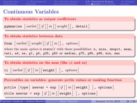
Continuous VariablesTo obtain statistics as output coefficients

summarize[varlist

][if

][in

][weight

][, detail

]To obtain statistics between data

fsum[varlist

][weight

][if

][in

][, options

]where the main option is stats() with these possibilities: n, miss, abspct, mean,vari, sd, se, p1, p5, p25, p50 or median, p75, p95, p99, min, max

To obtain statistics on the mean (like ci and se)

ci[varlist

][if

][in

][weight

] [, options

]Percentiles on variables: generate pctile values or ranking function

pctile[type

]newvar = exp

[if

][in

][weight

] [, options

]xtile newvar = exp

[if

][in

][weight

] [, options


C.I.D.E.


Continuous VariablesCompute the correlation (1)

correlate[varlist

][if

][in

][weight

][, correlate_options

]Compute the correlation (2)

pwcorr[varlist

][if

][in

][weight

][, pwcorr_options

]obs print the number of observations for each couple of variables

sig print the significance level of the correlation

star(#) display with the sign * significance levels less than #

bonferroni use Bonferroni-adjusted significance level

sidak use Sidak-adjusted significance level

Check for outliers

hadimvo varlist[if

][in

], generate(newvar1

[newvar2

])

[p(#)

]grubbs varlist

[if

][in

][, options

]drop eliminate the observations identified as outliers

generate(newvar1 ...) generate dummy variables for identifying outliers


C.I.D.E.


Discrete VariablesTable of frequences for single variable(s)

tabulate varname[if

][in

][weight

][, tabulate_options

]tab1 varlist

[if

][in

][weight

][, tab1_options

]missing include missing values

nolabel display numeric codes rather than value labels

sort display the table in descending order of frequency

Generate a table of counts, frequences and missing observations

fre[varlist

][if

][in

][weight

][, options

]nomissing omit missing values from the table

nolabel omit labels

include(numlist) include only values specified in numlist

ascending display rows in ascending order of frequency

descending display rows in discending order of frequency

tex export LaTeX-formatted tableFrancesco Andreoli - Andrea Bonfatti (Università di Verona)Stata Tutorial January 11-15, 2010 40 / 59

C.I.D.E.


Discrete VariablesCross-tabulation of 2 variables

tabulate varname1 varname2[if

][in

][weight

][, options

]chi2 report Pearson’s χ2

exact[(#)

]report Fisher’s exact test

gamma report Goodman and Kruskal’s gamma

column report the relative frequency within its column of each cell

row report the relative frequency within its row of each cell

cell report the relative frequency of each cell

nofreq do not display frequencies (use only with column, row or cell)

summarize(varname3) report summary statistics (mean, sd) for varname3

Cross-tabulation of more than 2 variables, by values

tab2 varlist[if

][in

][weight

][, options


C.I.D.E.


Tables of Statistics

table

table rowvar[colvar

[supercolvar

] ] [if

][in

][weight

][, options

]where in rowvar

[colvar

[supercolvar

] ]we put categorical variables (up to 3).

by(superrowvarlist) variables to be treated as superrows (up to 4)contents(clist) contents of the table’s cells, where clist may contain up to 5 statistics

mean varname meansd varname standard deviation

sum varname sumn varname count of nonmissing observations

max, min varname maximum and minimum valuemedian varname median

p1... p99 varname percentilesiqr varname interquartile range (p75-p25)


C.I.D.E.


Tables of Statisticstabstat

tabstat varlist[if

][in

][weight

][, by(varname) options

]where in varlist we place a list of continuous variables, in by(varname) a categoricalvariable and among the options in statistics() we can choose:

mean

n

sum

max, minsd

cv coefficient of variation (sd/mean)semean standard error of mean (sd/sqrt(n))

skewness index of skewnesskurtosis index of kurtosisp1... p99

range = max - miniqr interquartile range = p75 - p25


C.I.D.E.


Sample TestsTests apply to variables and allow to compare statistical significance of estimatesagainst a null hp on the whole sample observed or for its subgroups. You can alsouse the command to perform tests under subgroups mean equality for the samevariable, once a dicotomus variable identifying groups is selected (use missing valuesin this dummy varible to select only two subgroups which do not exhaust the sampledimension n). You can use the test_commandi to obtain t-tests from inputted data(n, sd, means) that you like to compare. Other more specific tests can bedownloaded and installed. Here is a list of general features:

Test for means equality: help ttest

Performs t-test for 1) one variable sample mean equality to a constant 2) onevariable two subsample means equality 3) two variables means equality 4) twovariables two subsample means equality. You can specify distributions.

Test for standard deviations equality: help sdtest

Performs t-test for 1) one variable sample sd equality to a constant 2) one variabletwo subsample sd equality 3) two variables sd equality 4) two variables twosubsample sd equality. You can specify distributions.


C.I.D.E.


Graphshelp graph

This is the general command for all graphs. From here you can start searching thegraphic style that you need, for univariate or multivariate representations, as well asstatistical constructions. This is the broadest family of graphics.

help twoway

This command applies to bivariate graphics. The objective is to obtain a classical 2coordinates graph, like scatter plots, connected points, confidence intervals,regression fit, distributions... One graph may contain different series (ex: timeagainst income and consumption) or different objects (ex: observed and predictedvalues). Once twoway is declared, you have to select (in pairs) the variables that youwant to put in the same graph and the type of graph linking the two variables (ex:scatter; connected; lfit; tsline; bar; spike; mband; lpoly;function;...). In this way, graphs are built sequentially and all the objectswill appear in the same space. You can add graphs options by looking at the help.Using by(), you obtain separeted graphs according to the variable you want to beconditioned to. Options and in, if must be specified for each graphic tool you use,bacause they refer to a particular set of data in use.


C.I.D.E.


Regression AnalysisStata econometrics models can be included into 5 large families, but only the firstone will be analysed. You are invited to read on the help the full characterization ofcommands. In each help file you also find examples and interpretations of outputresults.

1) Cross-section econometrics

You are invited to look at help regress for the admissible regression commands,including OLS, IV, limited dependent variables methods, treatment effects models,censoring and selection bias corrections, 3SLS, systems of equations, quantileregression. Using the command help regress_postestimation you also obtaininformation on post-estimation tests and model application syntax.

2) Time series econometrics

You are invited to look at help time, you will find all the list of commandsassociated with time series estimations, and how to build econometrics models inStata. In particular, help tsset can be used to declare a time series structure ofyour data, and than proceed with usual regression techniques. Using the commandhelp regress_postestimationts you also obtain information on post-estimationtests and model application syntax.


C.I.D.E.


Regression Analysis

3) Panel data econometrics

You are invited to look at help xt, you will find all the list of commandsassociated with the panel dimesion of a database. In particular, help xtregoffers a wide explanation of panel-data analysis techniques, while with helpxtreg_postestimation you also obtain information on post-estimation testsand model application syntax.

4) Survey data analysis

See help survey for all the details on data setting and regression techniques

5) Spatial econometrics

See help spatreg or spatwmat for geographically located data. Commandsavailable for Stata 10 or superior.


C.I.D.E.


Regression Analysis

Common models: OLS, IV, probit, multiple logit

regress depvar[indepvars

] [if

][in

][weight

][, noc options

]ivregress estimator depvar

[varlist1

](varlist2=varlist_iv)[

if][in

][weight

][, noc options

]probit depvar

[indepvars

] [if

][in

][weight

][, options

]mlogit depvar

[indepvars

] [if

][in

][weight

][, options

]options refers to regression specific options or estimation

correction (robust se, constant...)estimator IV can be performed by 2SLS, GMM or limited info max

likelihood.


C.I.D.E.


Regression AnlysisOther regression models: List I

areg an easier way to fit regressions with many dummy variables

arch regression models with ARCH errors

arima ARIMA models

boxcox Box-Cox regression models

cnreg censored-normal regression

cnsreg constrained linear regression

eivreg errors-in-variables regression

frontier stochastic frontier models

heckman Heckman selection model

intreg interval regression

ivregress single-equation instrumental-variables regression

ivtobit tobit regression with endogenous variables

newey regression with Newey-West standard errors

qreg quantile (including median) regression

reg3 three-stage least-squares (3SLS) regression

rreg a type of robust regression

sureg seemingly unrelated regression


C.I.D.E.


Regression AnlysisOther regression models: List II

tobit tobit regression

treatreg treatment-effects model

truncreg truncated regression

xtabond Arellano-Bond linear dynamic panel-data estimation

xtdpd linear dynamic panel-data estimation

xtfrontier panel-data stochastic frontier model

xtgls panel-data GLS models

xthtaylor Hausman-Taylor estimator for error-components models

xtintreg panel-data interval regression models

xtivreg panel-data instrumental variables (2SLS) regression

xtpcse linear regression with panel-corrected standard errors

xtreg fixed- and random-effects linear models

xtregar fixed- and random-effects linear models with an AR(1) disturbance

xttobit panel-data tobit modelsFrancesco Andreoli - Andrea Bonfatti (Università di Verona)Stata Tutorial January 11-15, 2010 50 / 59

C.I.D.E.


Post EstimationAny Post Estimation command must be used immediately after aregression model, and in any case it refers to last estimates stored inStata memory. You can save any model with a name and then proceedin post estimations recalling the model name.Predict calculates predictions, residuals, influence statistics, and thelike after estimation

Predict regression output as new data

predict[type

]newvar

[if

][in

][, statistic

]statistic

xb linear prediction; the defaultresiduals residuals

rstandard standardized residualsrstudent studentized (jackknifed) residuals

stdp standard error of the linear predictionstdr standard error of the residual


C.I.D.E.


Post EstimationTest linear hypothesis on coefficients

test coeflist

test exp=exp[=...

]Test on residuals: normality and zero-mean

sktest varname

ttest varname = 0

acatter/mband

Test on residuals: heteroskedasticity by graph and tests

rvplot

estat hettest

estat imtest

whitetst


C.I.D.E.


Post Estimation

Test on variables: influential values

dfbeta

Logic of the dfbeta test:1 Estimation with the complete sample2 Estimation without the i-th observation3 Comparison

Test on variables: collinearity

vif

collin

NOTE: values of VIF > 10 deserve attention


C.I.D.E.


Output: Interpreting

Results from computations are showed in the Results Window and stored inmemory by the .log file. You can paste your output directly on your paper(or in other spreadsheet to rework them) by using the tables reported in the.log file. Stata offers other opportunites to list estimates and coefficients in aproper way (ex. with standard errors between brackets) whithout requiringadditional changes in estimates values. In this Programming section we willsee how output coefficients, vectors (ex. the regression parameters), matrices(ex. the variance-covariance matrix of regression coefficients) or scalars (ex.the mean of a variable, its standard deviation, or an R2 estimation) can beproperly represented and used. By matrix algebra, we can perform advancedeconometrics on data.Remember that all the syntax previously presented applies exclusively todata stored in memory. To apply this syntax to your output coefficients (forexample compute the average of average values obtained by bootstrapping)you need to transform your results in data format (i.e. add columns).


C.I.D.E.


Show EstimatesYour code must be operable even after that changes in your data occurs (by mergeor append). Therefore, you need to perform your tests or report coefficientsindependently from your output windows results (ex: t-test for means). Stataallows to save the estimates as scalars or vectors/matrices. The general procedure isthe following:

1 Perform your statistical procedures or your estimations (like summarize orregress);

2 Save your results and estimates in the memory by using r() or e()respectively. In this way you generate a new object;

3 Use your objects or display them in the output files.

Alternatively, save regression results

outreg[varlist

]using filename

[, options

]text opt.: nol; title(); addn()coefficients opt.: bdec(); coefstarsignificance opt.: se | p | ci | beta; bracket; 3asterstat opt.: addstat(r2, N, F); xstatsother opt.: replace; append


C.I.D.E.


Show Estimates

See help postest for a general description of post estimationscommands. help estimates provides all the info to store, use andreport estimates. All commands work iff there is some result stored inthe memory.

Show estimatesAfter statistics: see help returnAfter regressions: see help ereturn

Scalar define, after summary statistics or table are reported

scalar[define

]scalar_name = exp

scalar list scalar_list

scalar drop scalar_list


C.I.D.E.


Show EstimatesAfter a regression command, use:

To store estimates in the memory (use name of your model)

estimates store name[, nocopy

]estimates dir

scalar drop name_list

To report statistics and estimates tables from model name

estimates stats namelist[, n(#)

]estimates table

[namelist

], options

stats(N r2 ll chi2 aic bic rank) reports statistics in the table;keep(coeflist); drop(coeflist) to eliminate some coeff from the table;b(%9.2f), se, t, p specify the format of coeff reported and additioal stats;

To use results

t(names); r(coef); r(stats)Francesco Andreoli - Andrea Bonfatti (Università di Verona)Stata Tutorial January 11-15, 2010 57 / 59

C.I.D.E.


Work with Data as Matrices

Data can be exported as a matrix n× k (a vector is a single columnmatrix), any statistics or estimation can be performed and result listedin the matrix format. New data created (ex., predictions) can betransformed in data from matrices.If you operate with matrices, use algebra to compute statistics (ex.X̄ = (e′e)−1e′X), any other command will not be working. If youtransform matrices in data (see the data editor), you can use previouslyseen commands. Use help matrix for an exhaustive review ofcommands to be used. To perform more complicated computation orbuild your program, use the Mata environment which allows to useStata more interactively. See help mata for review of commands,available in Stata 9 or superior.


C.I.D.E.


Work with Data as Matrices

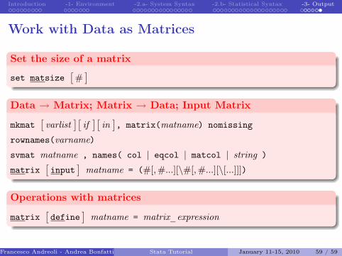
Set the size of a matrix

set matsize[

#]

Data → Matrix; Matrix → Data; Input Matrix

mkmat[varlist

][if

][in

], matrix(matname) nomissing

rownames(varname)

svmat matname , names( col | eqcol | matcol | string )

matrix[input

]matname = (#[, #...][\#[, #...][\[...]]])

Operations with matrices

matrix[define

]matname = matrix_expression


Stata Tutorial IT2010 - DSEdse.univr.it/it/documents/it5/stata_tutorial.pdf · ......

Documents

Transcript of Stata Tutorial IT2010 - DSEdse.univr.it/it/documents/it5/stata_tutorial.pdf · ......