Stata TutorialUpdated for Version 15

http://data.princeton.edu/stata

Germán RodríguezPrinceton University

July 2017

1. Introduction

Stata is a powerful statistical package with smart data-management facilities,a wide array of up-to-date statistical techniques, and an excellent system forproducing publication-quality graphs. Stata is fast and easy to use. In thistutorial I start with a quick introduction and overview and then discuss datamanagement, statistical graphs, and Stata programming.

The tutorial has been updated for version 15, but most of the discussion appliesto versions 8 and later. Version 14 added Unicode support, which will comehandy when we discuss multilingual labels in Section 2.3. Version 15 includes,among many new features, graph color transparency or opacity, which we’ll usein Section 3.3.

1.1 A Quick Tour of Stata

Stata is available for Windows, Unix, and Mac computers. This tutorial focuseson the Windows version, but most of the contents applies to the other platformsas well. The standard version is called Stata/IC (or Intercooled Stata) and canhandle up to 2,047 variables. There is a special edition called Stata/SE thatcan handle up to 32,766 variables (and also allows longer string variables andlarger matrices), and a version for multicore/multiprocessor computers calledStata/MP, which allows larger datasets and is substantially faster. The numberof observations is limited by your computer’s memory, as long as it doesn’texceed about two billion in Stata/SE and about a trillion in Stata/MP. Thereare versions of Stata for 32-bit and 64-bit computers; the latter can handlemore memory (and hence more observations) and tend to be faster. All of theseversions can read each other’s files within their size limits. (There used to be asmall version of Stata, limited to about 1,000 observations on 99 variables, butas of version 15 it is no longer available.)

1

Local Note: At OPR you can access Stata/SE on Windows by runningthe network version on your own workstation, just create a shortcut to\\opr\shares\applications\stata15-se\stataSE.exe. (If you have a 64-bitworkstation change the program name to stataSE-64.exe.) For computationallyintensive jobs you may want to login to our Windows server Coale via remotedesktop and run Stata/SE there. If you prefer Unix systems logon to our Unixserver lotka via X-Windows and leave your job running there.

1.1.1 The Stata Interface

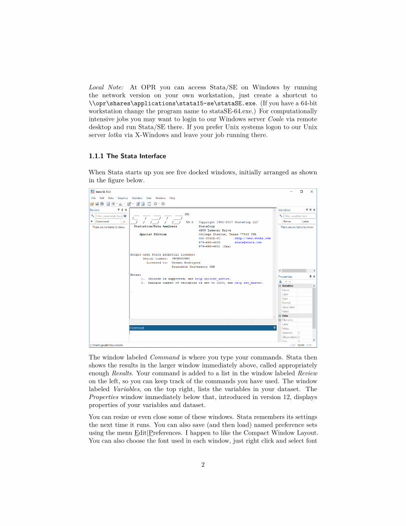
When Stata starts up you see five docked windows, initially arranged as shownin the figure below.

The window labeled Command is where you type your commands. Stata thenshows the results in the larger window immediately above, called appropriatelyenough Results. Your command is added to a list in the window labeled Reviewon the left, so you can keep track of the commands you have used. The windowlabeled Variables, on the top right, lists the variables in your dataset. TheProperties window immediately below that, introduced in version 12, displaysproperties of your variables and dataset.

You can resize or even close some of these windows. Stata remembers its settingsthe next time it runs. You can also save (and then load) named preference setsusing the menu Edit|Preferences. I happen to like the Compact Window Layout.You can also choose the font used in each window, just right click and select font

2

from the context menu; my own favorite on Windows is Lucida Console. Finally,it is possible to change the color scheme, selecting from seven preset or threecustomizable styles. One of the preset schemes is classic, the traditional blackbackground used in earlier versions of Stata.

There are other windows that we will discuss as needed, namely the Graph,Viewer, Variables Manager, Data Editor, and Do file Editor.

Starting with version 8 Stata’s graphical user interface (GUI) allows selectingcommands and options from a menu and dialog system. However, I stronglyrecommend using the command language as a way to ensure reproducibility ofyour results. In fact, I recommend that you type your commands on a separatefile, called a do file, as explained in Section 1.2 below, but for now we will justtype in the command window. The GUI can be helpful when you are startingto learn Stata, particularly because after you point and click on the menus anddialogs, Stata types the corresponding command for you.

1.1.2 Typing Commands

Stata can work as a calculator using the display command. Try typing thefollowing (excluding the dot at the start of a line, which is how Stata marks thelines you type):

. display 2+24. display 2 * ttail(20, 2.1).04861759

Stata commands are case-sensitive, display is not the same as Display and thelatter will not work. Commands can also be abbreviated; the documentationand online help underlines the shortest legal abbreviation of each command andwe will do the same here.

The second command shows the use of a built-in function to compute a p-value,in this case twice the probability that a Student’s t with 20 d.f. exceeds 2.1.This result would just make the 5% cutoff. To find the two-tailed 5% criticalvalue try display invttail(20, 0.025). We list a few other functions youcan use in Section 2.

If you issue a command and discover that it doesn’t work press the Page Upkey to recall it (you can cycle through your command history using the PageUp and Page Down keys) and then edit it using the arrow, insert and deletekeys, which work exactly as you would expect. For example Arrows advance acharacter at a time and Ctrl-Arrows advance a word at a time. Shift-Arrowsselect a character at a time and Shift-Ctrl-Arrows select a word at a time, whichyou can then delete or replace. A command can be as long as needed (up tosome 64k characters); in an interactive session you just keep on typing and thecommand window will wrap and scroll as needed.

3

1.1.3 Getting Help

Stata has excellent online help. To obtain help on a command (or function) typehelp command_name, which displays the help on a separate window called theViewer. (You can also type chelp command_name, which shows the help on theResults window; but this is not recommended.) Or just select Help|Command onthe menu system. Try help ttail. Each help file appears in a separate viewertab (a separate window before Stata 12) unless you use the option , nonew.

If you don’t know the name of the command you need, you can search for it.Stata has a search command that will search the documentation and otherresources, type help search to learn more. By default this command searchesthe net in Stata 13 and later. If you are using an earlier version learn about thefindit command. Also, the help command reverts to a search if the argumentis not recognized as a command. Try help Student's t. This will list allStata commands and functions related to the t distribution. Among the list of“Stat functions” you will see t() for the distribution function and ttail() forright-tail probabilities. Stata can also compute tail probabilities for the normal,chi-squared and F distributions, among others.

One of the nicest features of Stata is that, starting with version 11, all thedocumentation is available in PDF files. (In fact it looks as if starting withversion 13 you can no longer get printed manuals.) Moreover, these files arelinked from the online help, so you can jump directly to the relevant section ofthe manual. To learn more about the help system type help help.

1.1.4 Loading a Sample Data File

Stata comes with a few sample data files. You will learn how to read yourown data into Stata in Section 2, but for now we will load one of the samplefiles, namely lifeexp.dta, which has data on life expectancy and gross nationalproduct (GNP) per capita in 1998 for 68 countries. To see a list of the filesshipped with Stata type sysuse dir. To load the file we want type sysuselifeexp (the file extension is optional). To see what’s in the file type describe.(This command can be abbreviated to a single letter, but I prefer desc.)

. sysuse lifeexp, clear(Life expectancy, 1998). descContains data from C:\Program Files (x86)\Stata15\ado\base/l/lifeexp.dta

obs: 68 Life expectancy, 1998vars: 6 26 Mar 2016 09:40size: 2,652 (_dta has notes)

storage display valuevariable name type format label variable label

region byte %12.0g region Regioncountry str28 %28s Country

4

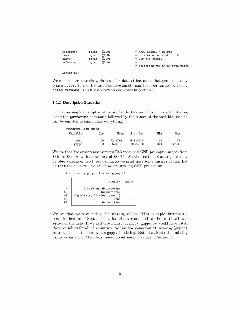
popgrowth float %9.0g * Avg. annual % growthlexp byte %9.0g * Life expectancy at birthgnppc float %9.0g * GNP per capitasafewater byte %9.0g *

* indicated variables have notes

Sorted by:

We see that we have six variables. The dataset has notes that you can see bytyping notes. Four of the variables have annotations that you can see by typingnotes varname. You’ll learn how to add notes in Section 2.

1.1.5 Descriptive Statistics

Let us run simple descriptive statistics for the two variables we are interested in,using the summarize command followed by the names of the variables (whichcan be omitted to summarize everything):

. summarize lexp gnppcVariable Obs Mean Std. Dev. Min Max

lexp 68 72.27941 4.715315 54 79gnppc 63 8674.857 10634.68 370 39980

We see that live expectancy averages 72.3 years and GNP per capita ranges from$370 to $39,980 with an average of $8,675. We also see that Stata reports only63 observations on GNP per capita, so we must have some missing values. Letus list the countries for which we are missing GNP per capita:

. list country gnppc if missing(gnppc)

country gnppc

7. Bosnia and Herzegovina .40. Turkmenistan .44. Yugoslavia, FR (Serb./Mont.) .46. Cuba .56. Puerto Rico .

We see that we have indeed five missing values. This example illustrates apowerful feature of Stata: the action of any command can be restricted to asubset of the data. If we had typed list country gnppc we would have listedthese variables for all 68 countries. Adding the condition if missing(gnppc)restricts the list to cases where gnppc is missing. Note that Stata lists missingvalues using a dot. We’ll learn more about missing values in Section 2.

5

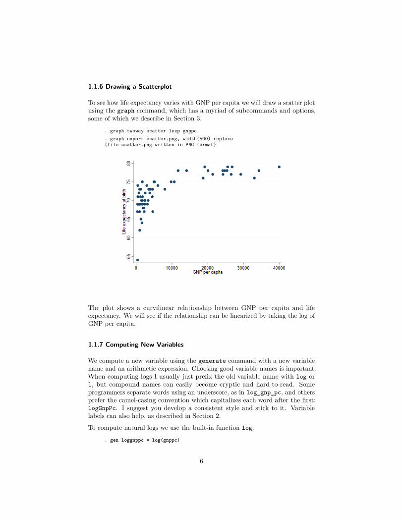
1.1.6 Drawing a Scatterplot

To see how life expectancy varies with GNP per capita we will draw a scatter plotusing the graph command, which has a myriad of subcommands and options,some of which we describe in Section 3.

. graph twoway scatter lexp gnppc

. graph export scatter.png, width(500) replace(file scatter.png written in PNG format)

The plot shows a curvilinear relationship between GNP per capita and lifeexpectancy. We will see if the relationship can be linearized by taking the log ofGNP per capita.

1.1.7 Computing New Variables

We compute a new variable using the generate command with a new variablename and an arithmetic expression. Choosing good variable names is important.When computing logs I usually just prefix the old variable name with log orl, but compound names can easily become cryptic and hard-to-read. Someprogrammers separate words using an underscore, as in log_gnp_pc, and othersprefer the camel-casing convention which capitalizes each word after the first:logGnpPc. I suggest you develop a consistent style and stick to it. Variablelabels can also help, as described in Section 2.

To compute natural logs we use the built-in function log:

. gen loggnppc = log(gnppc)

6

(5 missing values generated)

Stata says it has generated five missing values. These correspond to the fivecountries for which we were missing GNP per capita. Try to confirm thisstatement using the list command. We will learn more about generating newvariables in Section 2.

1.1.8 Simple Linear Regression

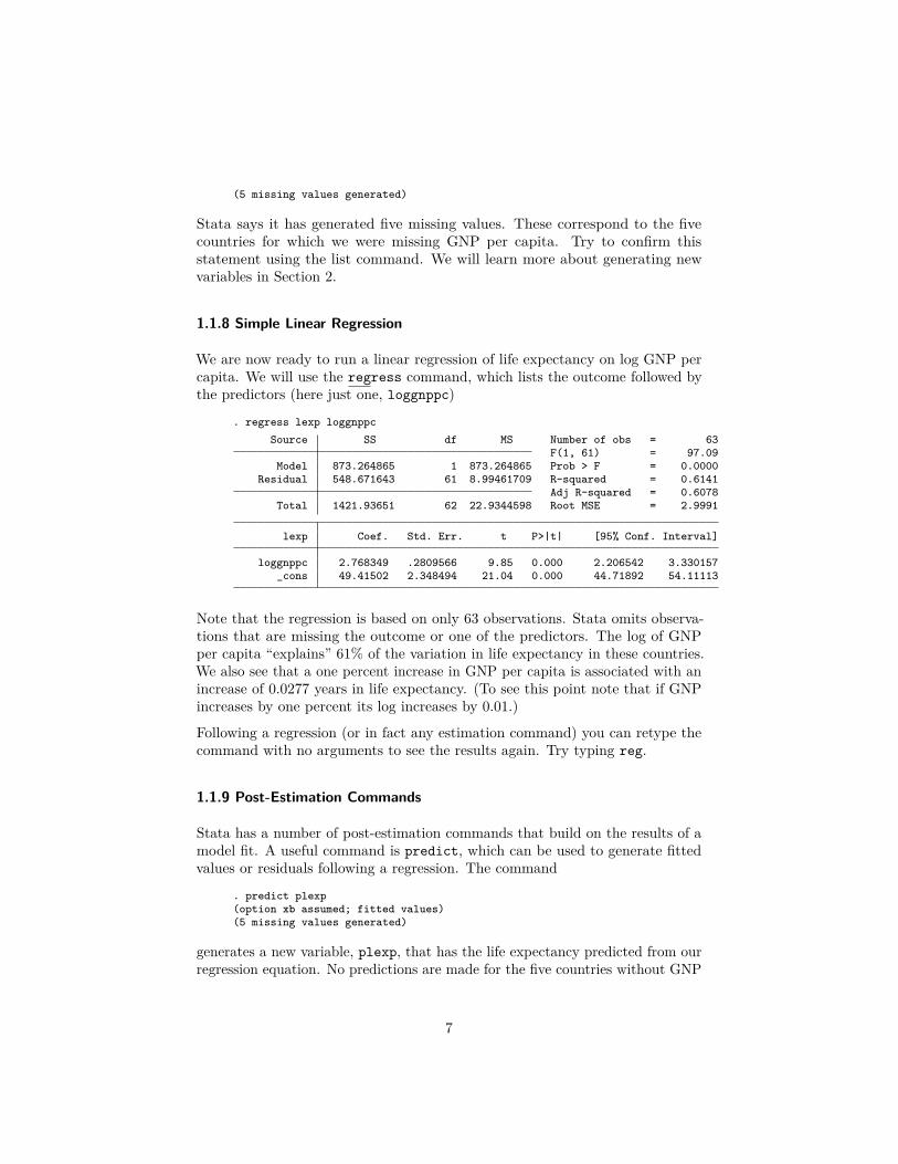
We are now ready to run a linear regression of life expectancy on log GNP percapita. We will use the regress command, which lists the outcome followed bythe predictors (here just one, loggnppc)

. regress lexp loggnppcSource SS df MS Number of obs = 63

F(1, 61) = 97.09Model 873.264865 1 873.264865 Prob > F = 0.0000

Residual 548.671643 61 8.99461709 R-squared = 0.6141Adj R-squared = 0.6078

Total 1421.93651 62 22.9344598 Root MSE = 2.9991

lexp Coef. Std. Err. t P>|t| [95% Conf. Interval]

loggnppc 2.768349 .2809566 9.85 0.000 2.206542 3.330157_cons 49.41502 2.348494 21.04 0.000 44.71892 54.11113

Note that the regression is based on only 63 observations. Stata omits observa-tions that are missing the outcome or one of the predictors. The log of GNPper capita “explains” 61% of the variation in life expectancy in these countries.We also see that a one percent increase in GNP per capita is associated with anincrease of 0.0277 years in life expectancy. (To see this point note that if GNPincreases by one percent its log increases by 0.01.)

Following a regression (or in fact any estimation command) you can retype thecommand with no arguments to see the results again. Try typing reg.

1.1.9 Post-Estimation Commands

Stata has a number of post-estimation commands that build on the results of amodel fit. A useful command is predict, which can be used to generate fittedvalues or residuals following a regression. The command

. predict plexp(option xb assumed; fitted values)(5 missing values generated)

generates a new variable, plexp, that has the life expectancy predicted from ourregression equation. No predictions are made for the five countries without GNP

7

per capita. (If life expectancy was missing for a country it would be excludedfrom the regression, but a prediction would be made for it. This technique canbe used to fill-in missing values.)

1.1.10 Plotting the Data and a Linear Fit

A common task is to superimpose a regression line on a scatter plot to inspectthe quality of the fit. We could do this using the predictions we stored in plexp,but Stata’s graph command knows how to do linear fits on the fly using the lfitplot type, and can superimpose different types of twoway plots, as explained inmore detail in Section 3. Try the command

. graph twoway (scatter lexp loggnppc) (lfit lexp loggnppc)

. graph export fit.png, width(500) replace(file fit.png written in PNG format)

In this command each expression in parenthesis is a separate two-way plot to beoverlayed in the same graph. The fit looks reasonably good, except for a possibleoutlier.

1.1.11 Listing Selected Observations

It’s hard not to notice the country on the bottom left of the graph, which hasmuch lower life expectancy than one would expect, even given its low GNP percapita. To find which country it is we list the (names of the) countries wherelife expectancy is less than 55:

8

. list country lexp plexp if lexp < 55, cleancountry lexp plexp

50. Haiti 54 66.06985

We find that the outlier is Haiti, with a life expectancy 12 years less than onewould expect given its GNP per capita. (The keyword clean after the comma isan option which omits the borders on the listing. Many Stata commands haveoptions, and these are always specified after a comma.) If you are curious wherethe United States is try

. list gnppc loggnppc lexp plexp if country == "United States", cleangnppc loggnppc lexp plexp

58. 29240 10.28329 77 77.88277

Here we restricted the listing to cases where the value of the variable countrywas “United States”. Note the use of a double equal sign in a logical expression.In Stata x = 2 assigns the value 2 to the variable x, whereas x == 2 checks tosee if the value of x is 2.

1.1.12 Saving your Work and Exiting Stata

To exit Stata you use the exit command (or select File|Exit in the menu, orpress Alt-F4, as in most Windows programs). If you have been following alongthis tutorial by typing the commands and try to exit Stata will refuse, saying“no; data in memory would be lost”. This happens because we have added a newvariable that is not part of the original dataset, and it hasn’t been saved. Asyou can see, Stata is very careful to ensure we don’t loose our work.

If you don’t care about saving anything you can type exit, clear, which tellsStata to quit no matter what. Alternatively, you can save the data to diskusing the save filename command, and then exit. A cautious programmer willalways save a modified file using a new name.

1.2 Using Stata Effectively

While it is fun to type commands interactively and see the results straightaway,serious work requires that you save your results and keep track of the commandsthat you have used, so that you can document your work and reproduce it laterif needed. Here are some practical recommendations.

1.2.1 Create a Project Directory

Stata reads and saves data from the working directory, usually C:\DATA, un-less you specify otherwise. You can change directory using the command cd[drive:]directory_name, and print the (name of the) working directory using

9

pwd, type help cd for details. I recommend that you create a separate directoryfor each course or research project you are involved in, and start your Statasession by changing to that directory.

Stata understands nested directory structures and doesn’t care if youuse \ or / to separate directories. Versions 9 and later also understandthe double slash used in Windows to refer to a computer, so you can cd\\opr\shares\research\myProject to access a shared project folder. Analternative approach, which also works in earlier versions, is to use Windowsexplorer to assign a drive letter to the project folder, for example assignP: to \\opr\shares\research\myProject and then in Stata use cd p:.Alternatively, you may assign R: to \\opr\shares\research and then use cdR:\myProject, a more convenient solution if you work in several projects.

Stata has other commands for interacting with the operating system, includingmkdir to create a directory, dir to list the names of the files in a directory, typeto list their contents, copy to copy files, and erase to delete a file. You can (andprobably should) do these tasks using the operating system directly, but theStata commands may come handy if you want to write a program to performrepetitive tasks.

1.2.2 Open a Log File

So far all our output has gone to the Results window, where it can be viewed buteventually disappears. (You can control how far you can scroll back, type helpscrollbufsize to learn more.) To keep a permanent record of your results,however, you should log your session. When you open a log, Stata writes allresults to both the Results window and to the file you specify. To open a log fileuse the command

log using filename, text replace

where filename is the name of your log file. Note the use of two recommendedoptions: text and replace.

By default the log is written using SMCL, Stata Markup and Control Language(pronounced “smickle”), which provides some formatting facilities but can onlybe viewed using Stata’s Viewer. Fortunately, there is a text option to createlogs in plain text format, which can be viewed in an editor such as Notepad ora word processor such as Word. (An alternative is to create your log in SMCLand then use the translate command to convert it to plain text, postscript, oreven PDF, type help translate to learn more about this option.)

The replace option specifies that the file is to be overwritten if it already exists.This will often be the case if (like me) you need to run your commands severaltimes to get them right. In fact, if an earlier run has failed it is likely that youhave a log file open, in which case the log command will fail. The solution isto close any open logs using the log close command. The problem with this

10

solution is that it will not work if there is no log open! The way out of the catch22 is to use

capture log close

The capture keyword tells Stata to run the command that follows and ignoreany errors. Use judiciously!

1.2.3 Always Use a Do File

A do file is just a set of Stata commands typed in a plain text file. You can useStata’s own built-in do-file Editor, which has the great advantage that you canrun your program directly from the editor by clicking on the run icon, selectingTools|Execute (do) from the menu, or using the shortcut Ctrl-D. The runicon can also be used to run selected commands and does it smartly: if you haveselected some text it will extend the selection to include complete lines and thenwill run those commands, if there is no selection it runs the entire script. Toaccess Stata’s do editor use Ctrl-9 in versions 12 and later (Ctrl-8 in earlierversions) or select Window|Do-file Editor|New Do-file Editor in the menusystem.

Alternatively, you can use an editor such as Notepad. Save the file using extension.do and then execute it using the command do filename. For a thoroughdiscussion of alternative text editors see http://fmwww.bc.edu/repec/bocode/t/textEditors.html, a page maintained by Nicholas J. Cox, of the University ofDurham.

You could even use a word processor such as Word, but you would have toremember to save the file in plain text format, not in Word document format.Also, you may find Word’s insistence on capitalizing the first word on each lineannoying when you are trying to type Stata commands that must be in lowercase.You can, of course, turn auto-correct off. But it’s a lot easier to just use aplain-text editor.

1.2.4 Use Comments and Annotations

Code that looks obvious to you may not be so obvious to a co-worker, or even toyou a few months later. It is always a good idea to annotate your do files withexplanatory comments that provide the gist of what you are trying to do.

In the Stata command window you can start a line with a * to indicate that itis a comment, not a command. This can be useful to annotate your output.

In a do file you can also use two other types of comments: // and /* */.

// is used to indicate that everything that follows to the end of the line is acomment and should be ignored by Stata. For example you could write

11

gen one = 1 // this will serve as a constant in the model

/* */ is used to indicate that all the text between the opening /* and the closing*/, which may be a few characters or may span several lines, is a comment tobe ignored by Stata. This type of comment can be used anywhere, even in themiddle of a line, and is sometimes used to “comment out” code.

There is a third type of comment used to break very long lines, as explained inthe next subsection. Type help comments to learn more about comments.

It is always a good idea to start every do file with comments that include atleast a title, the name of the programmer who wrote the file, and the date.Assumptions about required files should also be noted.

1.2.5 Continuation Lines

When you are typing on the command window a command can be as long asneeded. In a do-file you will probably want to break long commands into linesto improve readability.

To indicate to Stata that a command continues on the next line you use ///,which says everything else to the end of the line is a comment and the commanditself continues on the next line. For example you could write

graph twoway (scatter lexp loggnppc) ///(lfit lexp loggnppc)

Old hands might writegraph twoway (scatter lexp loggnppc) /**/ (lfit lexp loggnppc)

which “comments out” the end of the line.

An alternative is to tell Stata to use a semi-colon instead of the carriage returnat the end of the line to mark the end of a command, using #delimit ;, as inthis example:

#delimit ;graph twoway (scatter lexp loggnppc)

(lfit lexp loggnppc) ;

Now all commands need to terminate with a semi-colon. To return to usingcarriage return as the delimiter use

#delimit cr

The delimiter can only be changed in do files. But then you always use do files,right?

12

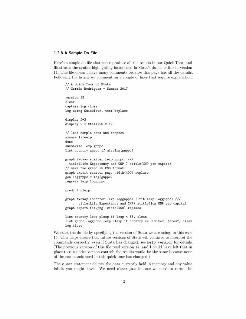
1.2.6 A Sample Do File

Here’s a simple do file that can reproduce all the results in our Quick Tour, andillustrates the syntax highlighting introduced in Stata’s do file editor in version11. The file doesn’t have many comments because this page has all the details.Following the listing we comment on a couple of lines that require explanation.

// A Quick Tour of Stata// Germán Rodríguez - Summer 2017

version 15clearcapture log closelog using QuickTour, text replace

display 2+2display 2 * ttail(20,2.1)

// load sample data and inspectsysuse lifeexpdescsummarize lexp gnppclist country gnppc if missing(gnppc)

graph twoway scatter lexp gnppc, ///title(Life Expectancy and GNP ) xtitle(GNP per capita)

// save the graph in PNG formatgraph export scatter.png, width(400) replacegen loggnppc = log(gnppc)regress lexp loggnppc

predict plexp

graph twoway (scatter lexp loggnppc) (lfit lexp loggnppc) ///, title(Life Expectancy and GNP) xtitle(log GNP per capita)

graph export fit.png, width(400) replace

list country lexp plexp if lexp < 55, cleanlist gnppc loggnppc lexp plexp if country == "United States", cleanlog close

We start the do file by specifying the version of Stata we are using, in this case15. This helps ensure that future versions of Stata will continue to interpret thecommands correctly, even if Stata has changed, see help version for details.(The previous version of this file read version 14, and I could have left that inplace to run under version control; the results would be the same because noneof the commands used in this quick tour has changed.)

The clear statement deletes the data currently held in memory and any valuelabels you might have. We need clear just in case we need to rerun the

13

program, as the sysuse command would then fail because we already have adataset in memory and we have not saved it. An alternative with the sameeffect is to type sysuse lifeexp, clear. (Stata keeps other objects in memoryas well, including saved results, scalars and matrices, although we haven’t hadoccasion to use these yet. Typing clear all removes these objects from memory,ensuring that you start with a completely clean slate. See help clear for moreinformation. Usually, however, all you need to do is clear the data.)

Note also that we use a graph export command to convert the graph in memoryto Portable Network Graphics (PNG) format, ready for inclusion in a web page.To include a graph in a Word document you are better off cutting and pasting agraph in Windows Metafile format, as explained in Section 3.

1.2.7 Stata Command Syntax

Having used a few Stata commands it may be time to comment briefly ontheir structure, which usually follows the following syntax, where bold indicateskeywords and square brackets indicate optional elements:

[by varlist:] command [varlist] [=exp] [if exp] [in range] [weight] [using filename][,options]

We now describe each syntax element:

command : The only required element is the command itself, which is usually (butnot always) an action verb, and is often followed by the names of one or morevariables. Stata commands are case-sensitive. The commands describeand Describe are different, and only the former will work. Commands canusually be abbreviated as noted earlier. When we introduce a commandwe underline the letters that are required. For example regress indicatesthat the regress command can be abbreviated to reg.

varlist : The command is often followed by the names of one or more variables,for example describe lexp or regress lexp loggnppc. Variable namesare case sensitive. lexp and LEXP are different variables. A variable namecan be abbreviated to the minimum number of letters that makes it uniquein a dataset. For example in our quick tour we could refer to loggnppcas log because it is the only variable that begins with those three letters,but this is a really bad idea. Abbreviations that are unique may becomeambiguous as you create new variables, so you have to be very careful. Youcan also use wildcards such as v* or name ranges, such as v101-v105 torefer to several variables. Type help varlist to lear more about variablelists.

=exp : Commands used to generate new variables, such as generate log_gnp= log(gnp), include an arithmetic expression, basically a formula usingthe standard operators (+ - * and / for the four basic operations and ˆ forexponentiation, so 3ˆ2 is three squared), functions, and parentheses. Wediscuss expressions in Section 2.

14

if exp and in range : As we have seen, a command’s action can be restrictedto a subset of the data by specifying a logical condition that evaluates totrue of false, such as lexp < 55. Relational operators are <, <=, ==,>= and >, and logical negation is expressed using ! or ~, as we will see inSection 2. Alternatively, you can specify a range of the data, for examplein 1/10 will restrict the command’s action to the first 10 observations.Type help numlist to learn more about lists of numbers.

weight : Some commands allow the use of weights, type help weights to learnmore.

using filename : The keyword using introduces a file name; this can be a filein your computer, on the network, or on the internet, as you will see whenwe discuss data input in Section 2.

options : Most commands have options that are specified following a comma.To obtain a list of the options available with a command type helpcommand. where command is the actual command name.

by varlist : A very powerful feature, it instructs Stata to repeat the commandfor each group of observations defined by distinct values of the variables inthe list. For this to work the command must be “byable” (as noted on theonline help) and the data must be sorted by the grouping variable(s) (oruse bysort instead).

1.3 Stata Resources

There are many resources available to learn more about Stata, both online andin print.

1.3.1 Online Resources

Stata has an excellent website at http://www.stata.com. Among other thingsyou will find that they make available online all datasets used in the officialdocumentation, that they publish a journal called The Stata Journal, andthat they have an excellent bookstore with texts on Stata and related statisticalsubjects. Stata also offers email and web-based training courses called NetCourses,see http://www.stata.com/netcourse/.

There is a Stata forum where you can post questions and receive prompt andknowledgeable answers from other users, quite often from the indefatigable andextremely knowledgeable Nicholas Cox, who deserves special recognition forhis service to the user community. The list was started by Marcello Paganoat the Harvard School of Public Health, and is now maintained by StataCorp,see http://www.statalist.org for more information, including how to participate.Stata also maintains a list of frequently asked questions (FAQ) classified bytopic, see http://www.stata.com/support/faqs/.

15

UCLA maintains an excellent Stata portal at http://www.ats.ucla.edu/stat/stata/, with many useful links, including a list of resources to help you learn andstay up-to-date with Stata. Don’t miss their starter kit, which includes “classnotes with movies”, a set of instructional materials that combine class notes withmovies you can view on the web, and their links by topic, which provides how-toguidance for common tasks. There are also more advanced learning modules,some with movies as well, and comparisons of Stata with other packages such asSAS and SPSS.

1.3.2 Manuals and Books

The Stata documentation has been growing with each version and now consistsof 27 volumes with more than 14,000 pages, all available in PDF format withyour copy of Stata. The basic documentation consists of a Base ReferenceManual, separate volumes on Data Management, Graphics, and Functions; aUser’s Guide, a Glossary and Index, and Getting Started with Stata, which hasplatform-specific versions for Windows, Macintosh and Unix. Some statisticalsubjects that may be important to you are described in sixteen separate manuals;here is a list, with italics indicating those new with Stata 15: Bayesian Analysis,Extended Regression Models, Finite Mixture Models, Item Response Theory,Linearized Dynamic Stochastic General Equilibrium, Longitudinal/Panel Data,Multilevel Mixed-Effects, Multiple Imputation, Multivariate Statistics, Powerand Sample Size, Spatial Autoregressive Models, Structural Equation Modeling,Survey Data, Survival Analysis and Epidemiological Tables, Times Series, andTreatment Effects. Additional volumes of interest to programmers, particularlythose seeking to extend Stata’s capabilities, are manuals on Programming andon Mata, Stata’s matrix programming language.

Good introductions to Stata include Alan C. Acock’s A Gentle Introduction toStata, now in its fifth edition, and Lawrence Hamilton’s Statistics with Stata(updated for version 12). One of my favorite statistical modeling books is ScottLong and Jeremy Freese’s Regression Models for Categorical Dependent VariablesUsing Stata (3rd edition); Section 2.10 of this book is a set of recommendedpractices that should be read and followed faithfully by every aspiring Statadata analyst. Another book I like is Michael Mitchell’s excellent A Visual Guideto Stata Graphics, which was written specially to introduce the new graphsin version 8 and is now in its 3rd edition. Two useful (but more specialized)references written by the developers of Stata are An Introduction to SurvivalAnalysis Using Stata (revised 3rd edition), by Mario Cleves, William Gouldand Julia Marchenko, and Maximum Likelihood Estimation with Stata (4thedition) by William Gould, Jeffrey Pitblado, and Brian Poi. Readers interestedin programming Stata will find Christopher F. Baum’s An Introduction to StataProgramming (2nd edition) invaluable.

16

2 Data Management

In this section I describe Stata data files, discuss how to read raw data intoStata in free and fixed formats, how to create new variables, how to document adataset labeling the variables and their values, and how to manage Stata systemfiles.

Stata 11 introduced a variables manager that allows editing variable names,labels, types, formats, and notes, as well as value labels, using an intuitivegraphical user interface available under Data|Variables Manager in the menusystem. While the manager is certainly convenient, I still prefer writing allcommands in a do file to ensure research reproducibility. A nice feature of themanager, however, is that it generates the Stata commands needed to accomplishthe changes, so it can be used as a learning tool and, as long as you are loggingthe session, leaves a record behind.

2.1 Stata Files

Stata datasets are rectangular arrays with n observations on m variables. Unlikepackages that read one observation at a time, Stata keeps all data in memory,which is one reason why it is so fast. There’s a limit of 2,047 variables inStata/IC, 32,767 in Stata/SE, and 120,000 in Stata/MP. You can have as manyobservations as your computer’s memory will allow, provided you don’t go toofar above 2 billion cases with Stata/SE and 1 trillion with Stata/MP. (To findthese limits type help limits.)

2.1.1 Variable Names

Variable names can have up to 32 characters, but many commands print only 12,and shorter names are easier to type. Stata names are case sensitive, Age andage are different variables! It pays to develop a convention for naming variablesand sticking to it. I prefer short lowercase names and tend to use single wordsor abbreviations rather than multi-word names, for example I prefer effortor fpe to family_planning_effort or familyPlanningEffort, although allfour names are legal. Note the use of underscores or camel casing to separatewords.

2.1.2 Variable Types

Variables can contain numbers or strings. Numeric variables can be stored asintegers (bytes, integers, or longs) or floating point (float or double). These typesdiffer in the range or precision of the values they can hold, type help datatypefor details.

17

You usually don’t need to be concerned about the storage mode; Stata doesall calculations using doubles, and the compress command will find the mosteconomical way to store each variable in your dataset, type help compress tolearn more.

You do have to be careful with logical comparisons involving floating point types.If you store 0.1 in a float called x you may be surprised to learn that x == 0.1is never true. The reason is that 0.1 is “rounded” to different binary numberswhen stored as a float (x) or as a double (the constant 0.1). This problem doesnot occur with integers or strings.

String variables can have varying lengths up to 244 characters in Stata 12, or up totwo billion characters in Stata 13 or higher, where you can use str1...str2045to define fixed-length strings of up to 2045 characters, and strL to define a longstring, suitable for storing plain text or even binary large objects such as imagesor word processing documents, type help strings to learn more. Strings areideally suited for id variables because they can be compared without problems.

Sometimes you may need to convert between numeric and string variables. Ifa variable has been read as a string but really contains numbers you will wantto use the command destring or the function real(). Otherwise, you canuse encode to convert string data into a numeric variable or decode to convertnumeric variables to strings. These commands rely on value labels, which aredescribed below.

2.1.3 Missing Values

Like other statistical packages, Stata distinguishes missing values. The basicmissing value for numeric variables is represented by a dot . Starting withversion 8 there are 26 additional missing-value codes denoted by .a to .z. Thesevalues are represented internally as very large numbers, so valid_numbers < . <.a < ... < .z.

To check for missing you need to write var >= . (not var == .). Stata has afunction that can do this comparison, missing(varname) and I recommend itbecause it leads to more readable code, e.g. I prefer list id if missing(age)to list id if age >= .

Missing values for string variables are denoted by “”, the empty string; not tobe confused with a string that is all blanks, such as " “.

Demographic survey data often use codes such as 88 for not applicable and 99 fornot ascertained. For example age at marriage may be coded 88 for single womenand 99 for women who are known to be married but did not report their ageat marriage. You will often want to distinguish these two cases using differentkinds of missing value codes. If you wanted to recode 88’s to .n (for “na” or notapplicable) and 99’s to .m (for “missing”) you could use the code

18

replace ageAtMar = .n if ageAtMar == 88replace ageAtMar = .m if ageAtMar == 99

Sometimes you want to tabulate a variable including missing values but excludingnot applicable cases. If you will be doing this often you may prefer to leave 99as a regular code and define only 88 as missing. Just be careful if you then runa regression!

Stata ships with a number of small datasets, type sysuse dir to get a list.You can use any of these by typing sysuse name. The Stata website is also arepository for datasets used in the Stata manuals and in a number of statisticalbooks.

2.2 Reading Data Into Stata

In this section we discuss how to read raw data files. If your data come fromanother statistical package, such as SAS or SPSS, consider using a tool suchas Stat/Transfer (www.stattransfer.com) or DBMSCopy (www.dataflux.com).Stata can read SAS transport files with the fdause command (so-named becausethis is the format required by the Food and Drug Administration), type helpfdause. Stata can also import and export Excel spreadsheets, type help importexcel to learn more, and can read data from relational databases, type helpodbc for an introduction.

2.2.1 Free Format

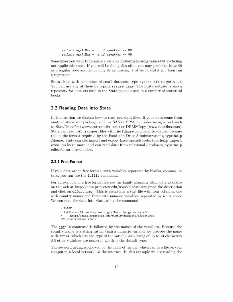
If your data are in free format, with variables separated by blanks, commas, ortabs, you can use the infile command.

For an example of a free format file see the family planning effort data availableon the web at http://data.princeton.edu/wws509/datasets (read the descriptionand click on effort.raw). This is essentially a text file with four columns, onewith country names and three with numeric variables, separated by white space.We can read the data into Stata using the command

. clear

. infile str14 country setting effort change using ///> http://data.princeton.edu/wws509/datasets/effort.raw(20 observations read)

The infile command is followed by the names of the variables. Because thecountry name is a string rather than a numeric variable we precede the namewith str14, which sets the type of the variable as a string of up to 14 characters.All other variables are numeric, which is the default type.

The keyword using is followed by the name of the file, which can be a file on yourcomputer, a local network, or the internet. In this example we are reading the

19

file directly off the internet. And that’s all there is to it. For more informationon this command type help infile1. To see what we got we can list a fewcases

. list in 1/3

country setting effort change

1. Bolivia 46 0 12. Brazil 74 0 103. Chile 89 16 29

Spreadsheet packages such as Excel often export data separated by tabs orcommas, with one observation per line. Sometimes the first line has the names ofthe variables. If your data are in this format you can read them using the importdelimited command. This command superseeded the insheet command as ofStata 13. Type help import delimited to learn more.

2.2.2 Fixed Format

Survey data often come in fixed format, with one or more records per case andeach variable in a fixed position in each record.

The simplest way to read fixed-format data is using the infix command tospecify the columns where each variable is located. As it happens, the effortdata are neatly lined up in columns, so we could read them as follows:

. infix str country 4-17 setting 23-24 effort 31-32 change 40-41 using ///> http://data.princeton.edu/wws509/datasets/effort.raw, clear(20 observations read)

This says to read the country name from columns 4-17, setting from columns23-24, and so on. It is, of course, essential to read the correct columns. Wespecified that country was a string variable but didn’t have to specify the width,which was clear from the fact that the data are in columns 4-17. The clearoption is used to overwrite the existing dataset in memory.

If you have a large number of variables you should consider typing the namesand locations on a separate file, called a dictionary, which you can then callfrom the infix command. Try typing the following dictionary into a file calledeffort.dct:

infix dictionary using http://data.princeton.edu/wws509/datasets/effort.raw {str country 4-17

setting 23-24effort 31-32change 40-41

}

20

Dictionaries accept only * comments and these must appear after the first line.After you save this file you can read the data using the command

infix using effort.dct, clear

Note that you now ‘use’ the dictionary, which in turn ‘uses’ the data file. Insteadof specifying the name of the data file in the dictionary you could specify it as anoption to the infix command, using the form infix using dictionaryfile,using(datafile). The first ‘using’ specifies the dictionary and the second‘using’ is an option specifying the data file. This is particularly useful if youwant to use one dictionary to read several data files stored in the same format.

If your observations span multiple records or lines, you can still read themusing infix as long as all observations have the same number of records (notnecessarily all of the same width). For more information see help infix.

The infile command can also be used with fixed-format data and a dictionary.This is a very powerful command that gives you a number of options not availablewith infix; for example it lets you define variable labels right in the dictionary,but the syntax is a bit more complicated. See help infile2.

In most cases you will find that you can read free-format data using infile andfixed-format data using infix. For more information on various ways to importdata into Stata see help import.

Data can also be typed directly into Stata using the input command, see helpinput, or using the built-in Stata data editor available through Data|Data editoron the menu system.

2.3 Data Documentation

After you read your data into Stata it is important to prepare some documenta-tion. In this section we will see how to create dataset, variable, and value labels,and how to create notes for the data or variables.

2.3.1 Data Label and Notes

Stata lets you label your dataset using the label data command followed by alabel of up to 80 characters (244 in Stata SE). You can also add notes of up to~64K characters each using the notes command followed by a colon and thenthe text:

. label data "Family Planning Effort Data"

. notes: Source P.W. Mauldin and B. Berelson (1978). ///> Conditions of fertility decline in developing countries, 1965-75. ///> Studies in Family Planning, 9:89-147

21

Users of the data can type notes to see your annotation. Documenting yourdata carefully always pays off.

2.3.2 Variable Labels and Notes

You can (and should) label your variables using the label variable commandfollowed by the name of the variable and a label of up to 80 characters enclosedin quotes. With the infile command you can add these labels to the dictionary,which is a natural home for them. Otherwise you should prepare a do file withall the labels. Here’s how to define labels for the three variables in our dataset:

. label variable setting "Social Setting"

. label variable effort "Family Planning Effort"

. label variable change "Fertility Change"

Stata also lets you add notes to specific variables using the command notesvarname: text. Note that the command is followed by a variable name andthen a colon:

. notes change: Percent decline in the crude birth rate (CBR) ///> -the number of births per thousand population- between 1965 and 1975.

Type describe and then notes to check our work so far.

2.3.3 Value Labels

You can also label the values of categorical variables. Our dataset doesn’t haveany categorical variables but let’s create one. We will make a copy of the familyplanning effort variable and then group it into three categories, 0-4, 5-14 and15+, which represent weak, moderate and strong programs (the generate andrecode used in the first two lines are described in the next section, where wealso show how to accomplish all these steps with just one command):

. generate effortg = effort

. recode effortg 0/4=1 5/14=2 15/max=3(effortg: 20 changes made). label define effortg 1 "Weak" 2 "Moderate" 3 "Strong", replace. label values effortg effortg. label variable effortg "Family Planning Effort (Grouped)"

Stata has a two-step approach to defining labels. First you define a named labelset which associates integer codes with labels of up to 80 characters (244 in StataSE), using the label define command. Then you associate the set of labels witha variable, using the label values command. Often you use the same namefor the label set and the variable, as we did in our example.

22

One advantage of this approach is that you can use the same set of labels forseveral variables. The canonical example is label define yesno 1 "yes" 0"no", which can then be associated with all 0-1 variables in your dataset, using acommand of the form label values variablename yesno for each one. Whendefining labels you can omit the quotes if the label is a single word, but I preferto use them always for clarity.

Label sets can be modified using the options add or modify, listed using labeldir (lists only names) or label list (lists names and labels), and saved to a dofile using label save. Type help label to learn more about these options andcommands. You can also have labels in different languages as explained below.

2.3.4 Multilingual Labels*

(This sub-section can be skipped without loss of continuity.) A Stata file can storelabels in several languages and you can move freely from one set to another. Onelimitation of multi-language support in version 13 and earlier is that labels wererestricted to 7-bit ascii characters, so you couldn’t include letters with diacriticalmarks such as accents. This limitation was removed with the introduction ofUnicode support in Stata 14, so you can use diacritical marks and other non-asciicharacters, not just in labels but throughout Stata.

I’ll illustrate the idea by creating Spanish labels for our dataset. Following Statarecommendations we will use the ISO standard two-letter language codes, enfor English and es for Spanish.

First we use label language to rename the current language to en, and tocreate a new language set es:

. label language en, rename(language default renamed en). label language es, new(language es now current language)

If you type desc now you will discover that our variables have no labels! Wecould have copied the English ones by using the option copy, but that wouldn’tsave us any work in this case. Here are Spanish versions of the data and variablelabels:

. label data "Datos de Mauldin y Berelson sobre Planificación Familiar"

. label variable country "País"

. label variable setting "Indice de Desarrollo Social"

. label variable effort "Esfuerzo en Planificación Familiar"

. label variable effortg "Esfuerzo en Planificación Familiar (Agrupado)"

. label variable change "Cambio en la Tasa Bruta de Natalidad (%)"

These definitions do not overwrite the corresponding English labels, but coexistwith them in a parallel Spanish universe. With value labels you have to be a

23

bit more careful, however; you can’t just redefine the label set called effortgbecause it is only the association between a variable and a set of labels, not thelabels themselves, that is stored in a language set. What you need to do is definea new label set; we’ll call it effortg_es, combining the old name and the newlanguage code, and then associate it with the variable effortg:

. label define effortg_es 1 "Débil" 2 "Moderado" 3 "Fuerte"

. label values effortg effortg_es

You may want to try the describe command now. Try tabulating effort (outputnot shown).

table effortg

Next we change the language back to English and run the table again:label language entable effortg

For more information type help label_language.

2.4 Creating New Variables

The most important Stata commands for creating new variables aregenerate/replace and recode, and they are often used together.

2.4.1 Generate and Replace

The generate command creates a new variable using an expression that maycombine constants, variables, functions, and arithmetic and logical operators.Let’s start with a simple example: here is how to create setting squared:

. gen settingsq = setting^2.

If you are going to use this term in a regression you know that linear andquadratic terms are highly correlated. It may be a good idea to center thevariable (by subtracting the mean) before squaring it. Here we run summarizeusing quietly to suppress the output and retrieve the mean from the storedresult r(mean):

. quietly summarize setting

. gen settingcsq = (setting - r(mean))^2

Note that I used a different name for this variable. Stata will not let you overwritean existing variable using generate. If you really mean to replace the values ofthe old variable use replace instead. You can also use drop var_names to dropone or more variables from the dataset.

24

2.4.2 Operators and Expressions

The following table shows the standard arithmetic, logical and relational operatorsyou may use in expressions:

Arithmetic Logical Relational+ add ! not (also ~) == equal- subtract | or != not equal (also ~=)∗ multiply & and < less than/ divide <= less than or equalˆ raise to power > greater than+ string concatenation >= greater than or equal

Here’s how to create an indicator variable for countries with high-effort programs:generate hieffort1 = effort > 14

This is a common Stata idiom, taking advantage of the fact that logical ex-pressions take the value 1 if true and 0 if false. A common alternative is towrite

generate hieffort2 = 0replace hieffort2 = 1 if effort > 14

The two strategies yield exactly the same answer. Both will be wrong if there aremissing values, which will be coded as high effort because missing value codesare very large values, as noted in Section 2.1 above. You should develop a goodhabit of avoiding open ended comparisons. My preferred approach is to use

generate hieffort = effort > 14 if !missing(effort)

which gives true for effort above 14, false for effort less than or equal to 14, andmissing when effort is missing. Logical expressions may be combined using & for“and” or | for “or”. Here’s how to create an indicator variable for effort between5 and 14:

gen effort5to14 = (effort >=5 & effort <= 14)

Here we don’t need to worry about missing values, they are excluded by theclause effort <= 14.

2.4.3 Functions

Stata has a large number of functions, here are a few frequently-used mathemat-ical functions, type help mathfun to see a complete list:

abs(x) the absolute value of xexp(x) the exponential function of x

25

int(x) the integer obtained by truncating x towards zeroln(x) or log(x) the natural logarithm of x if x>0log10(x) the log base 10 of x (for x>0)logit(x) the log of the odds for probability x: logit(x) = ln(x/(1-x))max(x1,x2,. . . ,xn) the maximum of x1, x2, . . . , xn, ignoring missing valuesmin(x1,x2,. . . ,xn) the minimum of x1, x2, . . . , xn, ignoring missing valuesround(x) x rounded to the nearest whole numbersqrt(x) the square root of x if x >= 0

These functions are automatically applied to all observations when the argumentis a variable in your dataset.

Stata also has a function to generate random numbers (useful in simulation),namely uniform(). It also has an extensive set of functions to compute proba-bility distributions (needed for p-values) and their inverses (needed for criticalvalues), including normal() for the normal cdf and invnormal() for its inverse,see help density functions for more information. To simulate normally dis-tributed observations you can use

rnormal() // or invnormal(uniform())

There are also some specialized functions for working with strings, see helpstring functions, and with dates, see help date functions.

2.4.4 Recoding Variables

The recode command is used to group a numeric variable into categories.Suppose for example a fertility survey has age in single years for women aged 15to 49, and you would like to code it into 5-year age groups. You could, of course,use something like

gen age5 = int((age-15)/5)+1 if !missing(age)

but this only works for regularly spaced intervals (and is a bit cryptic). Thesame result can be obtained using

recode age (15/19=1) (20/24=2) (25/29=3) (30/34=4) ///(35/39=5) (40/44=6) (45/49=7), gen(age5)

Each expression in parenthesis is a recoding rule, and consist of a list or rangeof values, followed by an equal sign and a new value. A range, specified usinga slash, includes the two boundaries, so 15/19 is 15 to 19, which could also bespecified as 15 16 17 18 19 or even 15 16 17/19. You can use min to refer to thesmallest value and max to refer to the largest value, as in min/19 and 44/max.The parentheses can be omitted when the rule has the form range=value, butthey usually help make the command more readable.

Values are assigned to the first category where they fall. Values that are neverassigned to a category are kept as they are. You can use else (or *) as the last

26

clause to refer to any value not yet assigned. Alternatively, you can use missingand nonmissing to refer to unassigned missing and nonmissing values; thesemust be the last two clauses and cannot be combined with else.

In our example we also used the gen() option to generate a new variable, in thiscase age5; the default is to replace the values of the existing variable. I stronglyrecommend that you always use the gen option or make a copy of the originalvariable before recoding it.

You can also specify value labels in each recoding rule. This is simpler andless error prone that creating the labels in a separate statement. The optionlabel(label_name) lets you assign a name to the labels created (the default isthe same as the variable name). Here’s an example showing how to recode andlabel family planning effort in one step (compare with the four commands usedin Section 2.4.2 above).

recode effort (0/4=1 Weak) (5/14=2 Moderate) (15/max=3 Strong) ///, generate(efffortg) label(effortg)

It is often a good idea to cross-tabulate original and recoded variables to checkthat the transformation has worked as intended. (Of course this can only bedone if you have generated a new variable!)

2.5 Managing Stata Files

Once you have created a Stata system file you will want to save it on disk usingsave filename, replace, where the replace option, as usual, is needed only ifthe file already exists. To load a Stata file you have saved in a previous sessionyou issue the command use filename.

If there are temporary variables you do not need in the saved file you can dropthem (before saving) using drop varnames. Alternatively, you may specify thevariables you want to keep, using keep varnames. With large files you may wantto compress them before saving; this command looks at the data and storeseach variable in the smallest possible data type that will not result in loss ofprecision.

It is possible to add variables or observations to a Stata file. To add variablesyou use the merge commmand, which requires two (or more) Stata files, usuallywith a common id so observations can be paired correctly. A typical applicationis to add household information to an individual data file. Type help merge tolearn more.

To add observations to a file you use the append command, which requires thedata to be appended to be on a Stata file, usually containing the same variablesas the dataset in memory. You may, for example, have data for patients in oneclinic and may want to append similar data from another clinic. Type helpappend to learn more.

27

A related but more specialized command is joinby, which forms all pairwisecombinations of observations in memory with observations in an external dataset(see also cross).

3 Stata Graphics

Stata has excellent graphic facilities, accessible through the graph command,see help graph for an overview. The most common graphs in statistics are X-Yplots showing points or lines. These are available in Stata through the twowaysubcommand, which in turn has 42 sub-subcommands or plot types, the mostimportant of which are scatter and line. I will also describe briefly bar plots,available through the bar subcommand, and other plot types.

Stata 10 introduced a graphics editor that can be used to modify a graphinteractively. I do not recomment this practice, however, because it conflictswith the goals of documenting and ensuring reproducibility of all the steps inyour research.

All the graphs in this section (except where noted) use a custom scheme withblue titles and a white background, but otherwise should look the same as yourown graphs. I discuss schemes in Section 3.2.5.

3.1 Scatterplots

In this section I will illustrate a few plots using the data on fertility decline firstused in Section 2.1. To read the data from net-aware Stata type

. infile str14 country setting effort change ///> using http://data.princeton.edu/wws509/datasets/effort.raw, clear(20 observations read)

To whet your appetite, here’s the plot that we will produce in this section:

3.1.1 A Simple Scatterplot

To produce a simple scatterplot of fertility change by social setting you use thecommand

graph twoway scatter change setting

Note that you specify y first, then x. Stata labels the axes using the variablelabels, if they are defined, or variable names if not. The command may beabbreviated to twoway scatter, or just scatter if that is the only plot on thegraph. We will now add a few bells and whistles.

28

3.1.2 Fitted Lines

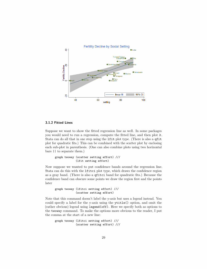
Suppose we want to show the fitted regression line as well. In some packagesyou would need to run a regression, compute the fitted line, and then plot it.Stata can do all that in one step using the lfit plot type. (There is also a qfitplot for quadratic fits.) This can be combined with the scatter plot by enclosingeach sub-plot in parenthesis. (One can also combine plots using two horizontalbars || to separate them.)

graph twoway (scatter setting effort) ///(lfit setting effort)

Now suppose we wanted to put confidence bands around the regression line.Stata can do this with the lfitci plot type, which draws the confidence regionas a gray band. (There is also a qfitci band for quadratic fits.) Because theconfidence band can obscure some points we draw the region first and the pointslater

graph twoway (lfitci setting effort) ///(scatter setting effort)

Note that this command doesn’t label the y-axis but uses a legend instead. Youcould specify a label for the y-axis using the ytitle() option, and omit the(rather obvious) legend using legend(off). Here we specify both as options tothe twoway command. To make the options more obvious to the reader, I putthe comma at the start of a new line:

graph twoway (lfitci setting effort) ///(scatter setting effort) ///

29

, ytitle("Fertility Decline") legend(off)

3.1.3 Labeling Points

There are many options that allow you to control the markers used for the points,including their shape and color, see help marker_options. It is also possibleto label the points with the values of a variable, using the mlabel(varname)option. In the next step we add the country names to the plot:

graph twoway (lfitci change setting) ///(scatter change setting, mlabel(country) )

One slight problem with the labels is the overlap of Costa Rica and TrinidadTobago (and to a lesser extent Panama and Nicaragua). We can solve thisproblem by specifying the position of the label relative to the marker using a12-hour clock (so 12 is above, 3 is to the right, 6 is below and 9 is to the left ofthe marker) and the mlabv() option. We create a variable to hold the positionset by default to 3 o’clock and then move Costa Rica to 9 o’clock and TrinidadTobago to just a bit above that at 11 o’clock (we can also move Nicaragua andPanama up a bit, say to 2 o’clock):

. gen pos=3

. replace pos = 11 if country == "TrinidadTobago"(1 real change made). replace pos = 9 if country == "CostaRica"(1 real change made). replace pos = 2 if country == "Panama" | country == "Nicaragua"(2 real changes made)

The command to generate this version of the graph is as followsgraph twoway (lfitci change setting) ///

(scatter change setting, mlabel(country) mlabv(pos) )

3.1.4 Titles, Legends and Captions

There are options that apply to all two-way graphs, including titles, labels,and legends. Stata graphs can have a title() and subtitle(), usually at thetop, and a legend(), note() and caption(), usually at the bottom, type helptitle_options to learn more. Usually a title is all you need. Stata 11 allowstext in graphs to include bold, italics, greek letters, mathematical symbols, anda choice of fonts. Stata 14 introduced Unicode, greatly expanding what can bedone. Type help graph text to learn more.

Our final tweak to the graph will be to add a legend to specify the linear fit and95% confidence interval, but not fertility decline itself. We do this using theorder(2 "linear fit" 1 "95% CI") option of the legend to label the secondand first items in that order. We also use ring(0) to move the legend inside the

30

plotting area, and pos(5) to place the legend box near the 5 o’clock position.Our complete command is then

. graph twoway (lfitci change setting) ///> (scatter change setting, mlabel(country) mlabv(pos) ) ///> , title("Fertility Decline by Social Setting") ///> ytitle("Fertility Decline") ///> legend(ring(0) pos(5) order(2 "linear fit" 1 "95% CI")). graph export fig31.png, width(500) replace(file fig31.png written in PNG format)

The result is the graph shown at the beginning of this section.

3.1.5 Axis Scales and Labels

There are options that control the scaling and range of the axes, includingxscale() and yscale(), which can be arithmetic, log, or reversed, type helpaxis_scale_options to learn more. Other options control the placing andlabeling of major and minor ticks and labels, such as as xlabel(), xtick() andxmtick(), and similarly for the y-axis, see help axis_label_options. Usuallythe defaults are acceptable, but it’s nice to know that you can change them.

3.2 Line Plots

I will illustrate line plots using data on U.S. life expectancy, available as one ofthe datasets shipped with Stata. (Try sysuse dir to see what else is available.)

. sysuse uslifeexp, clear(U.S. life expectancy, 1900-1999)

The idea is to plot life expectancy for white and black males over the 20thcentury. Again, to whet your appetite I’ll start by showing you the final product,and then we will build the graph bit by bit.

3.2.1 A Simple Line Plot

The simplest plot uses all the defaults:graph twoway line le_wmale le_bmale year

If you are puzzled by the dip before 1920, Google “US life expectancy 1918”. Wecould abbreviate the command to twoway line, or even line if that’s all weare plotting. (This shortcut only works for scatter and line.)

The line plot allows you to specify more than one “y” variable, the order isy1, y2, . . . , ym, x. In our example we specified two, corresponding to white andblack life expectancy. Alternatively, we could have used two line plots: (linele_wmale year) (line le_bmale year).

31

3.2.2 Titles and Legends

The default graph is quite good, but the legend seems too wordy. We will movemost of the information to the title and keep only ethnicity in the legend:

graph twoway line le_wmale le_bmale year ///, title("U.S. Life Expectancy") subtitle("Males") ///

legend( order(1 "white" 2 "black") )

Here I used three options, which as usual in Stata go after a comma: title,subtitle and legend. The legend option has many sub options; I used orderto list the keys and their labels, saying that the first line represented whites andthe second blacks. To omit a key you just leave it out of the list. To add textwithout a matching key use a hyphen (or minus sign) for the key. There aremany other legend options, see help legend_option to learn more.

I would like to use space a bit better by moving the legend inside the plot area,say around the 5 o’clock position, where improving life expectancy has left somespare room. As noted earlier we can move the legend inside the plotting area byusing ring(0), the “inner circle”, and place it near the 5 o’clock position usingpos(5). Because these are legend sub-options they have to go inside legend():

graph twoway line le_wmale le_bmale year ///, title("U.S. Life Expectancy") subtitle("Males") ///

32

legend( order(1 "white" 2 "black") ring(0) pos(5) )

3.2.3 Line Styles

I don’t know about you, but I find hard to distinguish the default lines on theplot. Stata lets you control the line style in different ways. The clstyle()option lets you use a named style, such as foreground, grid, yxline, or p1-p15for the styles used by lines 1 to 15, see help linestyle. This is useful if youwant to pick your style elements from a scheme, as noted further below.

Alternatively, you can specify the three components of a style: the line pattern,width and color:

• Patterns are specified using the clpattern() option. The most commonpatterns are solid, dash, and dot; see help linepatternstyle for moreinformation.

• Line width is specified using clwidth(); the available options include thin,medium and thick, see help linewidthstyle for more.

• Colors can be specified using the clcolor() option using color names(such as red, white and blue, teal, sienna, and many others) or RGBvalues, see help colorstyle.

Here’s how to specify blue for whites and red for blacks:graph twoway (line le_wmale le_bmale year , clcolor(blue red) ) ///

, title("U.S. Life Expectancy") subtitle("Males") ///legend( order(1 "white" 2 "black") ring(0) pos(5))

Note that clcolor() is an option of the line plot, so I put parentheses roundthe line command and inserted it there.

3.2.4 Scale Options

It looks as if improvements in life expectancy slowed down a bit in the secondhalf of the century. This can be better appreciated using a log scale, where astraight line would indicate a constant percent improvement. This is easily doneusing the axis options of the two-way command, see help axis_options, andin particular yscale(), which lets you choose arithmetic, log, or reversedscales. There’s also a suboption range() to control the plotting range. Here Iwill specify the y-range as 25 to 80 to move the curves a bit up:

. graph twoway (line le_wmale le_bmale year , clcolor(blue red) ) ///> , title("U.S. Life Expectancy") subtitle("Males") ///> legend( order(1 "white" 2 "black") ring(0) pos(5)) ///> yscale(log range(25 80))

33

3.2.5 Graph Schemes

Stata uses schemes to control the appearance of graphs, see help scheme. Youcan set the default scheme to be used in all graphs with set scheme_name. Youcan also redisplay the (last) graph using a different scheme with graph display,scheme(scheme_name).

To see a list of available schemes type graph query, schemes. Try s2color forscreen graphs, s1manual for the style used in the Stata manuals, and economistfor the style used in The Economist. Using the latter we obtain the graph shownat the start of this section.

. graph display, scheme(economist)

. graph export fig32.png, width(400) replace(file fig32.png written in PNG format)

3.3 Other Graphs

I conclude the graphics section discussing bar graphs, box plots, and kerneldensity plots using area graphs with transparency.

3.3.1 Bar Graphs

Bar graphs may be used to plot the frequency distribution of a categorical variable,or to plot descriptive statistics of a continuous variable within groups defined bya categorical variables. For our examples we will use the city temperature datathat ships with Stata.

If I was to just type graph bar, over(region) I would obtain the frequencydistribution of the region variable. Let us show instead the average tempera-tures in January and July. To do this I could specify (mean) tempjan (mean)tempjuly, but because the default statistic is the mean I can use the shorterversion below. I think the default legend is too long, so I also specified a customone.

I use over() so the regions are overlaid in the same graph; using by() instead,would result in a graph with a separate panel for each region. The bargap()option controls the gap between bars for different statistics in the same overgroup; here I put a small space. The gap() option, not used here, controls thespace between bars for different over groups. I also set the intensity of the colorfill to 70%, which I think looks nicer.

. sysuse citytemp, clear(City Temperature Data). graph bar tempjan tempjul, over(region) bargap(10) intensity(70) ///> title(Mean Temperature) legend(order(1 "January" 2 "July")). graph export bar.png, width(500) replace

34

(file bar.png written in PNG format)

Obviously the north-east and north-central regions are much colder in Januarythan the south and west. There is less variation in July, but temperatures arehigher in the south.

3.3.2 Box Plots

A quick summary of the distribution of a variable may be obtained using a“box-and-wiskers” plot, which draws a box ranging from the first to the thirdquartile, with a line at the median, and adds “wiskers” going out from the box tothe adjacent values, defined as the highest and lowest values that are no fartherfrom the median than 1.5 times the inter-quartile range. Values further out areoutliers, indicated by circles.

Let us draw a box plot of January temperatures by region. I will use theover(region) option, so the boxes will be overlaid in the same graph, ratherthan by(region), which would produce a separate panel for each region. Theoption sort(1) arranges the boxes in order of the median of tempjan, thefirst (and in this case only) variable. I also set the box color to a nice blue byspecifying the Red, Blue and Green (RGB) color components in a scale of 0 to255:

. graph box tempjan, over(region, sort(1)) box(1, color("51 102 204")) ///> title(Box Plots of January Temperature by Region). graph export boxplot.png, width(500) replace(file boxplot.png written in PNG format)

35

We see that January temperatures are lower and less variable in the north-eastand north-central regions, with quite a few cities with unusually cold averages.

3.3.3 Kernel Density Estimates

A more detailed view of the distribution of a variable may be obtained using asmooth histogram, calculated using a kernel density smoother using the kdensitycommand.

Let us run separate kernel density estimates for January temperatures in eachregion using all the defaults, and save the results.

. forvalues i=1/4 {2. capture drop x`i´ d`i´3. kdensity tempjan if region== `i´, generate(x`i´ d`i´)4. }

. gen zero = 0

Next we plot the density estimates using area plots with a floor at zero. Becausethe densities overlap, I use the new opacity option introduced in Stata 15 tomake them 50% transparent. In this case I used color names, followed by a %symbol and the opacity. I also simplify the legend a bit, match the order of thedensities, and put it in the top right corner of the plot.

. twoway rarea d1 zero x1, color("blue%50") ///> || rarea d2 zero x2, color("purple%50") ///> || rarea d3 zero x3, color("orange%50") ///> || rarea d4 zero x4, color("red%50") ///> title(January Temperatures by Region) ///

36

> ytitle("Smoothed density") ///> legend(ring(0) pos(2) col(1) order(2 "NC" 1 "NE" 3 "S" 4 "W")). graph export kernel.png, width(500) replace(file kernel.png written in PNG format)

The plot gives us a clear picture of regional differences in January temperatures,with colder and narrower distributions in the north-east and north-central regions,and warmer with quite a bit of overlap in the south and west.

3.4 Managing Graphs

Stata keeps track of the last graph you have drawn, which is stored in memory,and calls it “Graph”. You can actually keep more than one graph in memoryif you use the name() option to name the graph when you create it. This isuseful for combining graphs, type help graph combine to learn more. Notethat graphs kept in memory disappear when you exit Stata, even if you save thedata, unless you save the graph itself.

To save the current graph on disk using Stata’s own format, type graph savefilename. This command has two options, replace, which you need to use ifthe file already exists, and asis, which freezes the graph (including its currentstyle) and then saves it. The default is to save the graph in a live format thatcan be edited in future sessions, for example by changing the scheme. Aftersaving a graph in Stata format you can load it from the disk with the commandgraph use filename. (Note that graph save and graph use are analogous tosave and use for Stata files.) Any graph stored in memory can be displayed

37

using graph display [name]. (You can also list, describe, rename, copy, ordrop graphs stored in memory, type help graph_manipulation to learn more.)

If you plan to incorporate the graph in another document you will probably needto save it in a more portable format. Stata’s command graph export filenamecan export the graph using a wide variety of vector or raster formats, usuallyspecified by the file extension. Vector formats such as Windows metafile (wmfor emf) or Adobe’s PostScript and its variants (ps, eps, pdf) contain essentiallydrawing instructions and are thus resolution independent, so they are best forinclusion in other documents where they may be resized. Raster formats suchas Portable Network Graphics (png) save the image pixel by pixel using thecurrent display resolution, and are best for inclusion in web pages. Stata 15added Scalable Vector Graphics (SVG), a vector image format that is supportedby all major modern web browsers.

You can also print a graph using graph print, or copy and paste it into adocument using the Windows clipboard; to do this right click on the windowcontaining the graph and then select copy from the context menu.

4 Programming Stata

This section is a gentle introduction to programming Stata. I discuss macrosand loops, and show how to write your own (simple) programs. This is a largesubject and all I can hope to do here is provide a few tips that hopefully willspark your interest in further study. However, the material covered will help youuse Stata more effectively.

Stata 9 introduced a new and extremely powerful matrix programming languagecalled Mata. This extends the programmer’s tools well beyond the macrosubstitution tools discussed here, but Mata is a subject that deserves separatetreatment. Your efforts here will not be wasted, however, because Mata iscomplementary to, not a complete substitute for, classic Stata programming.

To learn more about programming Stata I recommend Kit Baum’s An Introduc-tion to Stata Programming, now in its second edition. You may also find usefulChapter 18 in the User’s Guide, referring to the Programming volume and/orthe online help as needed. Nick Cox’s regular columns in the Stata Journal area wonderful resource for learning about Stata. Other resources were listed inSection 1 of this tutorial.

4.1 Macros

A macro is simply a name associated with some text. Macros can be local orglobal in scope.

38

4.1.1 Storing Text in Local Macros

Local macros have names of up to 31 characters and are known only in thecurrent context (the console, a do file, or a program).

You define a local macro using local name [=] text and you evaluate it using`name'. (Note the use of a backtick or left quote.)

The first variant, without an equal sign, is used to store arbitrary text of upto ~64k characters (up to a million in Stata SE). The text is often enclosed inquotes, but it doesn’t have to be.

Example: Control Variables in Regression. You need to run a bunch of re-gression equations that include a standard set of control variables, say age,agesq, education, and income. You could, of course, type these names in eachequation, or you could cut and paste the names, but these alternatives aretedious and error prone. The smart way is to define a macro

local controls age agesq education income

You then type commands such asregress outcome treatment `controls'

which in this case is exactly equivalent to typing regress outcome treatmentage agesq education income.

If there’s only one regression to run you haven’t saved anything, but if you haveto run several models with different outcomes or treatments, the macro saveswork and ensures consistency.

This approach also has the advantage that if later you realize that you shouldhave used log-income rather than income as a control, all you need to do ischange the macro definition at the top of your do file, say to read logincomeinstead of income and all subsequent models will be run with income properlylogged (assuming these variables exist).

Warning: Evaluating a macro that doesn’t exist is not an error; it just returns anempty string. So be careful to spell macro names correctly. If you type regressoutcome treatment `contrls', Stata will read regress outcome treatment,because the macro contrls does not exist. The same would happen if you type`control' because macro names cannot be abbreviated the way variable namescan. Either way, the regression will run without any controls. But you alwayscheck your output, right?

Example: Managing Dummy Variables Suppose you are working with a de-mographic survey where age has been grouped in five-year groups and ends upbeing represented by seven dummies, say age15to19 to age45to49, six of whichwill be used in your regressions. Define a macro

39

local age "age20to24 age25to29 age30to34 age35to39 age40to44 age45to49"

and then in your regression models use something likeregress ceb `age' urban

which is not only shorter and more readable, but also closer to what you intend,which is to regress ceb on “age”, which happens to be a bunch of dummies. Thisalso makes it easier to change the representation of age; if you later decide touse linear and quadratic terms instead of the six dummies all you do is definelocal age "age agesq" and rerun your models. Note that the first occurrenceof age here is the name of the macro and the second is the name of a variable. Iused quotes to make the code clearer. Stata never gets confused.

Note on nested macros. If a macro includes macro evaluations, these are resolvedat the time the macro is created, not when it is evaluated. For example if youdefine local controls `age' income education. Stata sees that it includesthe macro age and substitutes the current value of age. Changing the contentsof the macro age at a later time does not change the contents of the macrocontrols.

There is, however, a way to achieve that particular effect. The trick is toescape the macro evaluation character when you define the macro, typing localcontrols \`age' income education. Now Stata does not evaluate the macro(but eats the escape character),so the contents of controls becomes `age'income education. When the controls macro is evaluated, Stata sees that itincludes the macro age and substitutes its current contents.

In one case substitution occurs when the macro is defined, in the other when itis evaluated.

4.1.2 Storing Results in Local Macros

The second type of macro definition, local name = text with an equal sign, isused to store results. It instructs Stata to treat the text on the right hand sideas an expression, evaluate it, and store a text representation of the result underthe given name.

Suppose you just run a regression and want to store the resulting R-squared, forcomparison with a later regression. You know that regress stores R-squared ine(r2), so you think local rsq e(r2) would do the trick.

But it doesn’t. Your macro stored the formula e(r2), as you can see by typingdisplay "`rsq'". What you needed to store was the value. The solution is totype local rsq = e(r2), with an equal sign. This causes Stata to evaluate theexpression and store the result.

To see the difference try this

. sysuse auto, clear

40

(1978 Automobile Data). quietly regress mpg weight. local rsqf e(r2). local rsqv = e(r2). di `rsqf´ // this has the current R-squared.65153125. di `rsqv´ // as does this.65153125. quietly regress mpg weight foreign. di `rsqf´ // the formula has the new R-squared.66270291. di `rsqv´ // this guy has the old one.65153125

Another way to force evaluation is to enclose e(r2) in single quotes when youdefine the macro. This is called a macro expression, and is also useful whenyou want to display results. It allows us to type display "R-squared=`rsqv'"instead of display "R-squared=" `rsq'. (What do you think would happenif you type display "``rsqf''"?)

An alternative way to store results for later use is to use scalars (type helpscalars to learn more.) This has the advantage that Stata stores the result inbinary form without loss of precision. A macro stores a text representation thatis good only for about 8 digits. The downside is that scalars are in the globalnamespace, so there is a potential for name conflicts, particular in programs(unless you use temporary names, which we discuss later).

You can use an equal sign when you are storing text, but this is not necessary, andis not a good idea if you are using an old version of Stata. The difference is subtle.Suppose we had defined the controls macro by saying local controls = "ageagesq education income". This would have worked fine, but the quotes causethe right-hand-side to be evaluated, in this case as a string, and strings used tobe limited to 244 characters (or 80 in Stata/IC before 9.1), whereas macro textcan be much longer. Type help limits to be reminded of the limits in yourversion.

4.1.3 Keyboard Mapping with Global Macros

Global macros have names of up to 32 characters and, as the name indicates,have global scope.

You define a global macro using global name [=] text and evaluate it using$name. (You may need to use ${name} to clarify where the name ends.)

I suggest you avoid global macros because of the potential for name conflicts. Auseful application, however, is to map the function keys on your keyboard. Ifyou work on a shared network folder with a long name try something like this

global F5 \\server\shared\research\project\subproject\

41

Then when you hit F5 Stata will substitute the full name. And your do files canuse commands like do ${F5}dofile. (We need the braces to indicate that themacro is called F5, not F5dofile.)

Obviously you don’t want to type this macro each time you use Stata. Solution?Enter it in your profile.do file, a set of commands that is executed each timeyou run Stata. Your profile is best stored in Stata’s start-up directory, usuallyC:\data. Type help profilew to learn more.

4.1.4 More on Macros

Macros can also be used to obtain and store information about the systemor the variables in your dataset using extended macro functions. For exampleyou can retrieve variable and value labels, a feature that can come handy inprogramming.

There are also commands to manage your collection of macros, including macrolist and macro drop. Type help macro to learn more.

4.2 Looping

Loops are used to do repetitive tasks. Stata has commands that allow loopingover sequences of numbers and various types of lists, including lists of variables.

Before we start, however, don’t forget that Stata does a lot of looping all byitself. If you want to compute the log of income, you can do that in Stata witha single line:

gen logincome = log(income)

This loops implicitly over all observations, computing the log of each income,in what is sometimes called a vectorized operation. You could code the loopyourself, but you shouldn’t because (i) you don’t need to, and (ii) your code willbe a lot slower that Stata’s built-in loop.

4.2.1 Looping Over Sequences of Numbers

The basic looping command takes the formforvalues number = sequence {

... body of loop using `number' ...}

Here forvalues is a keyword, number is the name of a local macro that will beset to each number in the sequence, and sequence is a range of values whichcan have the form

42

• min/max to indicate a sequence of numbers from min to max in steps ofone, for example 1/3 yields 1, 2 and 3, or

• first(step)last which yields a sequence from first to last in steps ofsize step. For example 15(5)50 yields 15,20,25,30,35,40,45 and 50.

(There are two other ways of specifying the second type of sequence, but I findthe one listed here the clearest, see help forvalues for the alternatives.)

The opening left brace must be the last thing on the first line (other thancomments), and the loop must be closed by a matching right brace on a line allby itself. The loop is executed once for each value in the sequence with yourlocal macro number (or whatever you called it) holding the value.

Creating Dummy Variables Here’s my favorite way of creating dummy vari-ables to represent age groups. Stata 11 introduced factor variables and Stata13 improved the labeling of tables of estimates, drastically reducing the need to“roll your own” dummies, but the code remains instructive.

forvalues bot = 20(5)45 {local top = `bot' + 4gen age`bot'to`top' = age >= `bot' & age <= `top'

}

This will create dummy variables age20to24 to age45to49. The way the loopworks is that the local macro bot will take values between 20 and 45 in steps of5 (hence 20, 25, 30, 35, 40, and 45), the lower bounds of the age groups.

Inside the loop we create a local macro top to represent the upper bounds ofthe age groups, which equals the lower bound plus 4. The first time through theloop bot is 20, so top is 24. We use an equal sign to store the result of adding 4to bot.

The next line is a simple generate statement. The first time through the loopthe line will say gen age20to24 = age >= 20 & age <= 24, as you can see bydoing the macro substitution yourself. This will create the first dummy, andStata will then go back to the top to create the next one.

4.2.2 Looping Over Elements in a List

The second looping command is foreach and comes in six flavors, dealing withdifferent types of lists. I will start with the generic list:

foreach item in a-list-of-things {... body of loop using `item' ...

}

Here foreach is a keyword, item is a local macro name of your own choosing,in is another keyword, and what comes after is a list of blank-separated words.Try this example

43

foreach animal in cats and dogs {display "`animal'"

}

This loop will print “cats”, “and”, and “dogs”, as the local macro animal is setto each of the words in the list. Stata doesn’t know “and” is not an animal, buteven if it did, it wouldn’t care because the list is generic.

If you wanted to loop over an irregular sequence of numbers –for example youneeded to do something with the Coale-Demeny regional model life tables forlevels 2, 6 and 12– you could write

foreach level in 2 6 12 {... do something with `level' ...

}

That’s it. This is probably all you need to know about looping.

4.2.3 Looping Over Specialized Lists

Stata has five other variants of foreach which loop over specific types of lists,which I now describe briefly.

Lists of Variables Perhaps the most useful variant isforeach varname of varlist list-of-variables {

... body of loop using `varname' ...}

Here foreach, of and varlist are keywords, and must be typed exactly as theyare. The list-of-variables is just that, a list of existing variable names typedusing standard Stata conventions, so you can abbreviate names (at your ownperil), use var* to refer to all variables that start with “var”, or type var1-var3to refer to variables var1 to var3.

The advantages of this loop over the generic equivalent foreach varname inlist-of-variables is that Stata checks that each name in the list is indeed anexisting variable name, and lets you abbreviate or expand the names.

If you need to loop over new as opposed to existing variables use foreachvarname of newlist list-of-new-variables. The newlist keyword re-places varlist and tells Stata to check that all the list elements are legal namesof variables that don’t exist already.

Words in Macros Two other variants loop over the words in a local or globalmacro; they use the keyword global or local followed by a macro name (inlieu of a list). For example here’s a way to list the control variables from thesection on local macros:

44

foreach control of local controls {display "`control'"

}

Presumably you would do something more interesting than just list the variablenames. Because we are looping over variables in the dataset we could haveachieved the same purpose using foreach with a varlist; here we save thechecking.

Lists of Numbers Stata also has a foreach variant that specializes in lists ofnumbers (or numlists in Stataspeak) that can’t be handled with forvalues.

Suppose a survey had a baseline in 1980 and follow ups in 1985 and 1995. (Theyactually planned a survey in 1990 but it was not funded.) To loop over theseyou could use

foreach year of numlist 1980 1985 1995 {display "`year'"

}

Of course you would do something more interesting than just print the years.The numlist could be specified as 1 2 3, or 1/5 (meaning 1 2 3 4 5), or 1(2)7(count from 1 to 7 in steps of 2 to get 1 3 5 7); type help numlist for moreexamples.

The advantage of this command over the generic foreach is that Stata will checkthat each of the elements of the list of numbers is indeed a number.

4.2.4 Looping for a While

In common with many programming languages, Stata also has a while loop,which has the following structure

while condition {... do something ...

}

where condition is an expression. The loop executes as long as the condition istrue (nonzero). Usually something happens inside the loop to make the conditionfalse, otherwise the code would run forever.

A typical use of while is in iterative estimation procedures, where you mayloop while the difference in successive estimates exceeds a predefined tolerance.Usually an iteration count is used to detect lack of convergence.

The continue [,break] command allows breaking out of any loop, includingwhile, forvalues and foreach. The command stops the current iteration andcontinues with the next, unless break is specified in which case it exits the loop.

45

4.2.5 Conditional Execution

Stata also has an if programming command, not to be confused with theifqualifier that can be used to restrict any command to a subset of the data, asin summarize mpg if foreign. The ifcommand has the following structure

if expression {... commands to be executed if expression is true ...

}else {

... optional block to be executed if expression is false ...}

Here if and the optional else are keywords, type help exp for an explanationof expressions. The opening brace { must be the last thing on a line (other thancomments) and the closing brace } must be on a new line by itself.

If the if or else parts consist of a single command they can go on the same linewithout braces, as in if expression command. But if expression { command} is not legal. You could use the braces by spreading the code into three linesand this often improves readability of the code.

So here we have a silly loop where we break out after five of the possible teniterations:

forvalues iter=1/10 {display "`iter'"if `iter' >= 5 continue, break

}

And with that, we break out of looping.

4.3 Writing Commands

We now turn to the fun task of writing your own Stata commands. Follow alongas we develop a couple of simple programs, one to sign your output, and anotherto evaluate the Coale-McNeil model nuptiality schedule, so we can create a plotlike the figure below.

4.3.1 Programs With No Arguments

Let us develop a command that helps label your output with your name. (Usuallyyou would want a timestamp, but that is already available at the top of your logfile. You always log your output, right?) The easiest way to develop a commandis to start with a do file. Fire up Stata’s do-file editor (Ctrl-8) and type:

capture program drop signprogram define sign

version 9.1

46

display as text "Germán Rodríguez "display "{txt}{hline 62}"

end

That’s it. If you now type sign Stata will display the signature using the textstyle (usually black on your screen).

The program drop statement is needed in case we make changes and need torerun the do file, because you can’t define an existing program. The capture isneeded the very first time, when there is nothing to drop.

The version statement says this command was developed for version 9.1 ofStata, and helps future versions of Stata run it correctly even if the syntax haschanged in the interim.

The last line uses a bit of SMCL, pronounced “smickle” and short for StataMarkup Control Language, which is the name of Stata’s output processor. SMCLuses plain text combined with commands enclosed in braces. For example {txt}sets display mode to text, and {hline 62} draws a horizontal rule exactly 62characters wide. To learn more about SMCL type help smcl.

4.3.2 A Program with an Argument

To make useful programs you will often need to pass information to them, inthe form of “arguments” you type after the command. Let’s write a commandthat echoes what you say

capture program drop echoprogram define echo

47

version 9.1display as text "`0'"

end

Try typing echo Programming Stata Tutorial to see what happens.

When you call a command Stata stores the arguments in a local macro called 0.We use a display command with `0' to evaluate the macro. The result is text,so we enclose it in quotes. (Suppose you typed echo Hi, so the local macro 0has Hi; the command would read display Hi and Stata will complain, saying‘Hi not found’. We want the command to read display "Hi", which is why wecode display "`0'".)

If we don’t specify anything, the local macro 0 will be an empty string, thecommand will read display "" and Stata will print a blank line.

4.3.3 Compound Quotes

Before we go out to celebrate we need to fix a small problem with our newcommand. Try typing echo The hopefully “final” run. Stata will complain.Why? Because after macro substitution the all-important display command willread

display "The hopefully "final" run"

The problem is that the quote before final closes the initial quote, so Stata seesthis is as The hopefully followed by final "run", which looks to Stata like aninvalid name. Obviously we need some way to distinguish the inner and outerquotes.

Incidentally you could see exactly where things went south by typing set traceon and running the command. You can see in (often painful) detail all the stepsStata goes through, including all macro substitutions. Don’t forget to type settrace off when you are done. Type help trace to learn more.

The solution to our problem? Stata’s compound double quotes: `" to openand "' to close, as in `"compound quotes"'. Because the opening and closingsymbols are different, these quotes can be nested. Compound quotes

• can be used anywhere a double quote is used.• must be used if the text being quoted includes double quotes.

So our program must display `"`0'"'. Here’s the final version.program define echo

version 9.1if `"`0'"' != "" display as text `"`0'"'

end

You will notice that I got rid of the capture drop line. This is because weare now ready to save the program as an ado file. Type sysdir to find out

48

where your personal ado directory is, and then save the file there with the nameecho.ado. The command will now be available any time you use Stata.

(As a footnote, you would want to make sure that there is no official Statacommand called echo. To do this I typed which echo. Stata replied “commandecho not found as either built-in or ado-file”. Of course there is no guaranteethat they will not write one; Stata reserves all english words.)

4.3.4 Positional Arguments

In addition to storing all arguments together in local macro 0, Stata parses thearguments (using white space as a delimiter) and stores all the words it finds inlocal macros 1, 2, 3, etc.

Typically you would do something with `1' and then move on to the next one.The command mac shift comes handy then, because it shifts all the macrosdown by one, so the contents of 2 is now in 1, and 3 is in 2, and so on. This wayyou always work with what’s in 1 and shift down. When the list is exhausted 1is empty and you are done.

So here is the canonical program that lists its argumentscapture program drop echoprogram define echo

version 9.1while "`1'" != "" {

display `"`1'"'mac shift

}end

Don’t forget the mac shift, otherwise your program may run forever. (Or untilyou hit the break key.)

Try echo one two three testing. Now try echo one "two and three"four. Notice how one can group words into a single argument by using quotes.

This method is useful, and sometimes one can given the arguments more mean-ingful names using args, but we will move on to the next level, which is a lotmore powerful and robust.

(By the way one can pass arguments not just to commands, but to do files aswell. Type help do to learn more.)

4.3.5 Using Stata Syntax

If your command uses standard Stata syntax, which means the arguments are alist of variables, possibly a weight, maybe an if or in clause, and perhaps a bunch

49

of options, you can take advantage of Stata’s own parser, which convenientlystores all these elements in local macros ready for you to use.

A Command Prototype Let us write a command that computes the probabilityof marrying by a certain age in a Coale-McNeil model with a given mean, standarddeviation, and proportion marrying. The syntax of our proposed command is

pnupt age, generate(married) [ mean(25) stdev(5) pem(1)]

So we require an existing variable with age in exact years, and a mandatoryoption specifying a new variable to be generated with the proportions married.There are also options to specify the mean, the standard deviation, and theproportion ever married in the schedule, all with defaults. Here’s a first cut atthe command

capture program drop pnuptprogram define pnupt

version 9.1syntax varname, Generate(name) ///

[ Mean(real 25) Stdev(real 5) Pem(real 1) ]// ... we don't do anything yet ...

end

The first thing to note is that the syntax command looks remarkably like ourprototype. That’s how easy this is.

Variable Lists The first element in our syntax is an example of a list of variablesor varlist. You can specify minima and maxima, for example a programrequiring exactly two variables would say varlist(min=2 max=2). When youhave only one variable, as we do, you can type varname, which is short forvarlist(min=1 max=1).

Stata will then make sure that your program is called with exactly one nameof an existing variable, which will be stored in a local macro called varlist.(The macro is always called varlist, even if you have only one variable andused varname in your syntax statement.) Try pnupt nonesuch and Stata willcomplain, saying “variable nonesuch not found”.

(If you have done programming before, and you spent 75% of your time writingchecks for input errors and only 25% focusing on the task at hand, you willreally appreciate the syntax command. It does a lot of error checking for you.)

Options and Defaults Optional syntax elements are enclosed in square brackets[ and ]. In our command the generate option is required but the other threeare optional. Try these commands to generate a little test dataset with an agevariable ranging from 15 to 50

50

drop _allset obs 36gen age = 14 + _n

Now try pnupt age. This time Stata is happy with age but notes ‘optiongenerate() required’. Did I say syntax saves a lot of work? Options that takearguments need to specify the type of argument (integer, real, string, name)and, optionally, a default value. Our generate takes a name, and is required, sothere is no default. Try pnupt age, gen(2). Stata will complain that 2 is nota name.

If all is well, the contents of the option is stored in a local macro with the samename as the option, here generate.

Checking Arguments Now we need to do just a bit of work to check that thename is a valid variable name, which we do with confirm:

confirm new variable `generate'

Stata then checks that you could in fact generate this variable, and if not issueserror 110. Try pnupt age, gen(age) and Stata will say ‘age already defined’.

It should be clear by now that Stata will check that if you specify a mean,standard deviation or proportion ever married, abbreviated as m(), s() andp(), they will be real numbers, which will be stored in local macros called mean„stdev, and pem. If an option is omitted the local macro will contain the default.

You could do more checks on the input. Let’s do a quick check that all threeparameters are non-negative and the proportion is no more than one.

if (`mean' <= 0 | `stdev' <= 0 | `pem' <= 0 | `pem' > 1) {di as error "invalid parameters"exit 110

}

You could be nicer to your users and have separate checks for each parameter,but this will do for now.

Temporary Variables We are now ready to do some calculations. We takeadvantage of the relation between the Coale-McNeil model and the gammadistribution, as explained in Rodríguez and Trussell (1980). Here’s a workingversion of the program

program define pnupt*! Coale-McNeil cumulative nuptiality schedule v1 GR 24-Feb-06

version 9.1syntax varname, Generate(name) [Mean(real 25) Stdev(real 5) Pem(real 1)]confirm new var `generate'if `mean' <= 0 | `stdev' <= 0 | `pem' <= 0 | `pem' > 1 {

display as error "invalid parameters"

51

exit 198}tempname z ggen `z' = (`varlist' - `mean')/`stdev'gen `g' = gammap(0.604, exp(-1.896 * (`z' + 0.805)))gen `generate' = `pem' * (1 - `g')

end

We could have written the formula for the probability in one line but only bysacrificing readability. Instead we first standardize age, by subtracting the meanand dividing by the standard deviation. What can we call this variable? Youmight be tempted to call it z, but what if the user of your program has a variablecalled z? Later we evaluate the gamma function. What can we call the result?

The solution is the tempname command, which asks Stata to make up uniquetemporary variable names, in this case two to be stored in local macros z andg. Because these macros are local, there is no risk of name conflicts. Anotherfeature of temporary variables is that they disappear automatically when yourprogram ends, so Stata does the housekeeping for you.

The line gen `z' = (`varlist' - `mean')/`stdev' probably looks a bitstrange at first. Remember that all quantities of interest are now stored in localmacros and we need to evaluate them to get anywhere, hence the profusion ofbackticks: `z' gets the name of our temporary variable, `varlist' gets thename of the age variable specified by the user, `mean' gets the value of the mean,and `stdev' gets the value of the standard deviation. After macro substitutionthis line will read something like gen _000001 = (age-22.44)/5.28, whichprobably makes a lot more sense.

If/In You might consider allowing the user to specify if and in conditions foryour command. These would need to be added to the syntax, where they wouldbe stored in local macros, which can then be used in the calculations, in thiscase passed along to generate.

For a more detailed discussion of this subject type help syntax and select ifand then in. The entry in help mark is also relevant.

4.3.6 Creating New Variables

Sometimes all your command will do is create a new variable. This, in fact, iswhat our little command does. Wouldn’t it be nice if we could use an egen typeof command like this:

egen married = pnupt(age), mean(22.48) stdev(5.29) pem(0.858)

Well, we can! As it happens, egen is user-extendable. To implement a functioncalled pnupt you have to create a program (ado file) called _gpnupt, in otherwords add the prefix _g. The documentation on egen extensions is a bit sparse,

52

but once you know this basic fact all you need to do is look at the source of anegen command and copy it. (I looked at _gmean.)

So here’s the egen version of our Coale-McNeil command.program define _gpnupt*! Coale-McNeil cumulative nuptiality schedule v1 GR 24-Feb-06

version 9.1syntax newvarname=/exp [, Mean(real 25) Stdev(real 5) Pem(real 1)]if `mean' <= 0 | `stdev' <= 0 | `pem' <= 0 | `pem' > 1 {

display as error "invalid parameters"exit 198

}tempname z ggen `z' = (`exp' - `mean')/`stdev'gen `g' = gammap(0.604, exp(-1.896 * (`z' + 0.805)))gen `typlist' `varlist' = `pem' * (1 - `g')

end

There are very few differences between this program and the previous one.Instead of an input variable egen accepts an expression, which gets evaluatedand stored in a temporary variable called exp. The output variable is specifiedas a varlist, in this case a newvarname. That’s why z now works with exp,and gen creates varlist. The mysterious typlist is there because egen letsyou specify the type of the output variable (float by default) and that getspassed to our function, which passes it along to gen.

4.3.7 A Coale-McNeil Fit

We are ready to reveal how the initial plot was produced. The data are availablein a Stata file in the demography section of my website, which has counts ofever married and single women by age. We compute the observed proportionmarried, compute fitted values based on the estimates in Rodríguez and Trussell(1980), and plot the results. It’s all done in a handful of lines

use http://data.princeton.edu/eco572/datasets/cohhnuptgen obs = ever/totalegen fit = pnupt(age+0.5), mean(22.44) stdev(5.28) pem(.858)gen agem = age + 0.5twoway (scatter obs agem) (line fit agem), ///

title(Proportions Married by Age) subtitle(Colombia 1976) ///ytitle(Proportion married) xtitle(age)

The actual estimation can be implemented using Stata’s maximum likelihoodprocedures, but that’s a story for another day.

53

4.4 Other Topics

For lack of time and space I haven’t discussed returning values from your program,type help return to learn more. For related subjects on estimation commandswhich can post estimation results see help ereturn and help _estimates. Anessential reference on estimation is Maximum Likelihood Estimation with Stata,Fourth Edition, by Gould, Pitblado and Poi (2010).

Other subjects of interest are matrices (start with help matrix), and how tomake commands “byable” (type help byable). For serious output you needto learn more about SMCL, start with help smcl. For work on graphics youmay want to study class programming (help class) and learn about sersets(help serset). To provide a graphical user interface to your command try helpdialog programming. It is possible to read and write text and binary files (seehelp file), but I think these tasks are better handled with Mata. You caneven write Stata extensions in C, but the need for those has also diminishedwith the availability of Mata.

Reference

Rodríguez G. and Trussell T.J. (1980). Maximum Likelihood Estimation of theParameters of Coale’s Model Nuptiality Schedule from Survey Data. WorldFertility Survey Technical Bulletins, 7.

54