Specification and derivation ofdigital circuits using...

Supervisor

Advisor

EINDHOVEN UNIVERSITY OF TECHNOLOGY

Department of Mathematics and Computing Science

MASTER'S THESIS

Specification and derivationof digital circuits

using higher-order logic

by

A. Raap

prof.dr.ir. C. J. Koomen

ir. P. J. de Graaff

October 9, 1990

Abstract

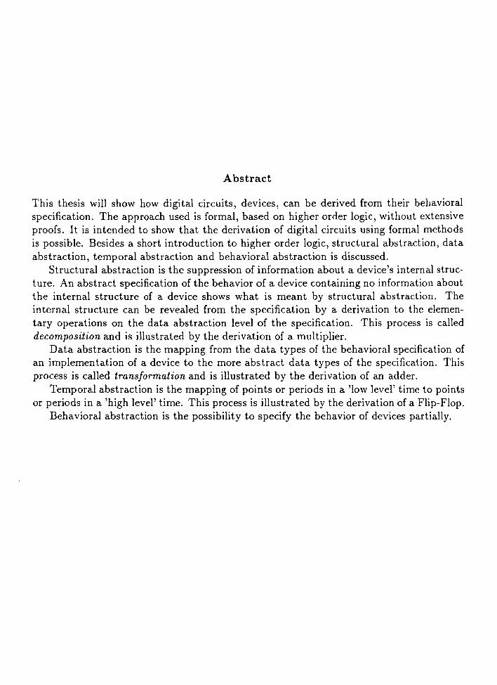
This thesis will show how digital circuits, devices, can be derived from their behavioralspecification. The approach used is formal, based on higher order logic, without extensiveproofs. It is intended to show that the derivation of digital circuits using formal methodsis possible. Besides a short introduction to higher order logic, structural abstraction, dataabstraction, temporal abstraction and behavioral abstraction is discussed.

Structural abstraction is the suppression of information about a device's internal structure. An abstract specification of the behavior of a device containing no information aboutthe internal structure of a device shows what is meant by structural abstraction. Theinternal structure can be revealed from the specification by a derivation to the elementary operations on the data abstraction level of the specification. This process is calleddecomposition and is illustrated by the derivation of a multiplier.

Data abstraction is the mapping from the data types of the behavioral specification ofan implementation of a device to the more abstract data types of the specification. Thisprocess is called transformation and is illustrated by the derivation of an adder.

Temporal abstraction is the mapping of points or periods in a 'low level' time to pointsor periods in a 'high level' time. This process is illustrated by the derivation of a Flip-Flop.

Behavioral abstraction is the possibility to specify the behavior of devices partially.

Contents

1 Introduction 31.1 Verification and derivation 3

1.1.1 Abstraction .. . . 41.1.2 Structural abstraction 61.1.3 Behavioral abstraction 61.1.4 Data abstraction ... 61.1.5 Temporal abstraction . 7

1.2 How this thesis is organized 7

2 Decomposition 82.1 Decomposition of a specification 82.2 Decomposition of a multiplier 82.3 Introducing internal states 11

3 The description formalism 143.1 Formal logic . . · . · . 143.2 First-order logic .. · . 14

3.2.1 Binding and substitution 163.2.2 Quantification . · . · . 183.2.3 Mathematical Induction 18

3.3 Higher-order logic . · . 183.3.1 Equality · . · . · . 183.3.2 Lambda expressions 183.3.3 Lambda reductions 19

4 Specification 214.1 A behavioral description · .. 214.2 Introduction of states. · .... 224.3 Transformation and decomposition 24

5 Types and typed terms 265.1 Partial ordering 265.2 Type operators · . 27

1

5.3 The basic types . . . . . . .5.4 The Cartesian product type5.5 The disjoint union type.5.6 Typed terms . . .5.7 The beel - type .5.8 The num - type

6 Transformation6.1 Type isomorphism .6.2 Transformation as type isomorphism6.3 Types for subsets of D(num)6.4 Implementations6.5 The adder . . . . . . . .

7 Signals and system timing7.1 Time .7.2 Signals .7.3 Behavior of a Flip-Flop7.4 Temporal abstraction ..

7.4.1 An example of temporal abstraction.7.4.2 Temporal abstraction of the Flip-Flop

7.5 Time representation in sequences .7.5.1 The type operator seq .

7.5.2 Sequences and functions over time.7.6 Behavioral abstraction .

8 Concluding remarks8.1 Specification and derivation .

8.1.1 The input type and output type .8.1.2 Abstract operations and specifications8.1.3 Derivation.

8.2 Conclusions . . . .8.3 Acknowledgements

2

292930303132

333335363839

4444454547484949495152

54545455555657

Chapter 1

Introduction

Recent advances in microelectronics make it possible to build electronic devices of unprecedented size and complexity. With increasing size and complexity, however, it becomesincreasingly difficult to ensure that such systems will not malfunction because of designerrors.

This problem has been the reason for many researchers to look for a firm theoreticalbasis for correct design of hardware systems. A specification of the behavior of electronicdevices is needed to be able to reason about correct implementations of electronic devices.This specification has to be expressed formally and concisely. Hardware design languages(HDL's) have been developed to express specifications and designs of electronic devices.

Hanna and Deach [HD86, p. 180] showed why a typed higher-order predicate logic[End72] is the best formalism for expressing the semantics of a Hardware Design Language(HDL) They have based their choice on the following criteria:

• the formalism already exists

• the formalism is powerful and concise

• the formalism allows informal and intuitive reasoning

• the formalism allows partial descriptions

• the formalism is strictly formal

1.1 Verification and derivation

Gordon has introduced a version of higher-order logic which can be used to prove digitalcircuits correct with respect to their specification [Gor86]. He expresses a digital circuitin a predicate ,·...hich is calculated from the specifications of the components of the circuit,the implementation, and compares it to the specification, which is also a predicate. If thespecification implies the implementation then the circuit is correct. De Graaff has shownthat there may be several implementations that satisfy the same specification and vice versa

3

[dG90]. Subrahmanyam and Herbert studied how to deal with timing and abstraction inhigher-order logic [Sub88, Her89]. The Hardware Verification Group at Cambridge havedeveloped the HOL-system, a theorem proving system for higher-order logic [GorSS]. Mostof the authors mentioned above have used this system to derive proofs. A different theoremprover is VERITAS, developed at the University of Kent [HD85].

Gordon's higher-order logic has proved to be useful. It complies to all criteria for aformalism for expressing a HDL, but it is focused on verification of existing digital circuits.Deriving digital circuits from a specification is something else. In what way does derivingdiffer from verifying? Proving the correctness of a design using hardware verificationtypically involves [MeIS8, p. 267]:

• \Vriting a set of formulas S which express the specification of the device whose designis to be proven correct.

• Describing the design or implementation of the device by a second set of formulas I.

• Proving that a 'satisfaction' or correctness relation holds between the sets of formulasI and S - i.e. that the implementation satisfies the specification.

This process is usually carried out at each level of the structural hierarchy of the design.The top level specification is shown to be satisfied by some connection of components; thespecification of these components are in turn shown to be satisfied by their implementations, and so on - until the level of primitive components is reached. If this technique isto be used to verify large and complex designs, it is clear that the 'satisfaction relation'that is used can not be strict equivalence. Otherwise, at each level of the design hierarchy,the specifications will contain all the information present in the design descriptions at thelevel below. For large and complex designs this means that the specifications at the upperlevels of the hierarchy will themselves become so large and complex that they can no longerbe seen to reflect the intended behavior of the device. Furthermore, proofs of equivalencewill become unmanageable.

A satisfaction or correctness relation based on the idea of abstraction, rather thanequivalence, is the key to making formal verification of large designs tractable. In thederivation process, a design or implementation of a device is found by deriving the implementation from a specification of the device. For large and complex designs derivationis manageable if the idea of abstraction, as described in [MeISS], is used. Derivation of aspecification has to match the informal modes of expression and intuitive reasoning [HD86,p. 180]. Johnson [Joh86] has shown that functional calculus is an appropriate basis forderiving digital circuits from their specifications. His idea will be used in the specificationof devices described in this thesis.

1.1.1 Abstraction

The idea of abstraction described below is due to [MeIS8]. Abstraction involves the suppression of irrelevant detail of information, in order to concentrate on the things of interest.

4

In hardware verification and derivation, the larger and more complex the system we aredescribing, the more irrelevant detail must be ignored to keep the specifications small.Thus, in general, specifications will be abstractions of the devices actually implemented.This means that the satisfaction or correctness relation that is used must involve abstraction mechanisms that, by removing information, relate the more detailed implementationdescriptions to their abstract specifications.

Example. The specification of a microprocessor, for example, would include a descriptionof the effect of each instruction on the machine registers. The description of a microcodedimplementation of the system would contain far more information, including the exactsequence of the microinstructions which implements each macroinstruction. To show thatthis design is correct, we would have to prove that each microcode sequence produces theeffect on the registers that is required by the specification of the corresponding macroinstruction. Here, the abstraction mechanism used to relate the levels of description is thecomposition of state changes; by composing a sequence of low level state changes to geta single transition, we 'hide' from the top level specification information about the intermediate state changes that occur during macroinstruction execution.

Derivation. In hardware derivation, an abstract description is derived from the specification. This description must contain only elementary operations where further derivationwithin the abstraction level of the specification is not useful. Then the related implementation description can be derived to one that contains elementary operations in theimplementation level. These operations can be derived on a lower implementation level,and so on - until the descriptions of primitive components is reached.

Example. In the example of the microprocessor, the macroinstruction is being derived toone or more elementary macroinstructions. For example, an addition of a value in memory,m, and the value in a register, r, can be replaced by reading the value m in the accumulatorfirst, and then add it to the value in r. Writing macroinstructions as microinstructions isdone on a lower level. At the abstract level, we only know what each instruction does; atthe more detailed implementation level, we also know how the instruction does it.

Suppose that we have proved the behavioral descriptions on an implementation levelof elementary operations on an abstract level correct with respect to their formal specifications. Then we can use these specifications to prove a behavioral description of a largerdevice correct with respect to the specification if the description consists the elementaryoperations on the abstract level. At the same time we have a 'translation' of the behavioral description to the implementation level. If we do this at each level of the proof ofa hierarchically structured design, we can control the size and complexity of the entireproof. In this way, abstraction mechanisms combine with hierarchical structuring to makeit possible to handle proofs of large systems.

Kinds of abstraction. There are four kinds of abstraction:

5

1. structural abstraction

2. behavioral abstraction

3. data abstraction

4. temporal abstraction

They will be discussed below.

1.1.2 Structural abstraction

The kind of abstraction most fundamental to hardware verification and derivation is structural abstraction - the suppression of information about a device's internal structure.The idea of structural abstraction is that the specification of a device should not reflectits internal construction, but only its externally observable behavior. The description of adevice's implementation, however, must contain explicit information about its structure;the mechanism of structural abstraction therefore involves formalizing the idea that suchinformation concerns 'internal' structure.

1.1.3 Behavioral abstraction

Behavioral abstraction concerns specifications that only partially define a device's behavior,leaving unspecified its behavior in certain states or for certain input values. Such partialspecification is appropriate. For example, when we know that a device will never haveto operate in certain environments then it is unnecessary to specify its expected behaviorin all environments. The mechanism of behavioral abstraction serves to relate partialspecifications to implementation descriptions that fully define the device's behavior, byshowing that they agree on the device's behavior for all states and inputs that are ofinterest, i.e. that are defined by the specification.

1.1.4 Data abstraction

The concept of data abstraction is well known from programming language theory. Thereare several abstract data types which are useful for formal specification of hardware; asimple example is the type of boolean truth values; a data abstraction from analog signalsroutinely used by hardware designers to reason about circuits. Another example is thetype of n-bit integers, represented at a less abstract level by vectors of booleans.

A data abstraction step consists of a mapping from the data types of an implementationdescription to more abstract data types of the specification. This mapping is then usedto show that the operations carried out on the low level data types correctly implementthe desired operations on the high level types. In the hardware derivation we only determine elementary operations on the high level data types and show that the correspondingoperations carried out on the low level data types correctly implement those operations.

6

Any complex operation expressed in elementary operations on high level data types canbe 'translated' to the low level data types because there are already correct 'translations'of the elementary operations in the high level data type to operations in low level datatypes. So it is not necessary to express complex operations in high level data types inoperations in low level data types if there are enough elementary operations in the highlevel data type.

1.1.5 Temporal abstraction

In temporal abstraction a sequential or time-dependent behavior of a device is viewedat different 'grains' of discrete time. An example of temporal abstraction is the unitdelay or register, implemented using an edge triggered flip flop. At the abstract level ofdescription the device is specified as a unit delay, one 'unit' discrete time corresponding tothe clock period; at the detailed level of description the grain of time is finer, several unitsof time corresponding to the delay through a gate. The proof of a microcoded computerdesign, mentioned above, also involves temporal abstraction; at the higher level there isone machine instruction step per unit of discrete time. Relating the levels of temporalabstraction involves mapping points or periods of low level time to points or periods ofhigh level time and showing that a many-step low level computation implements a one-stephigh level computation.

1.2 How this thesis is organized

This thesis will describe a method to derive implementations of digital circuits from anabstract specification of the behavior of the circuits. The four kinds of abstraction mentioned above will be explained using higher order logic. A short introduction to higherorder logic will be given and some examples will illustrate the kinds of abstraction used.

7

Chapter 2

Decomposition

How can we derive a behavioral description expressed in elementary operations from abehavioral specification of a circuit? To answer this question, we need to know what theelementary operations are.

Elementary operations. The behavior of elementary operations is specified within anabstraction level and has a description in a lower abstraction level such that the descriptionsatisfies the specification of the operation. If there is no lower abstraction level, then thedescription is expressed in primitive operations, that is, operations specifying primitiveelectronic devices like NAND-gates, inverters, et cetera.

If there is a lower abstraction level, then the behavioral description in the lower abstraction level is expressed in elementary operations in that level. Those elementary operationshave descriptions in another lower abstraction level, and so on - until the primitive abstraction level is reached.

2.1 Decomposition of a specification

The derivation of a specification to a behavioral description in elementary operations iscalled decomposition. Let us study an example.

Example. On IN, the set of all natural numbers, the operations defined on IN are addition(+), subtraction (-), multiplication (x) and the' div ' and' mod' operations. All theseoperations have to be constructed from elementary operations in a low level data type, first.The operation for multiplication can be constructed using the other elementary operationson IN. We will see this in the following section.

2.2 Decomposition of a multiplier

First, some mathematics is defined before a decomposition of a multiplier is derived. Wewill use the conditional (p -+ t lu) denoting 'if p then t else u'. Mathematical induction will

8

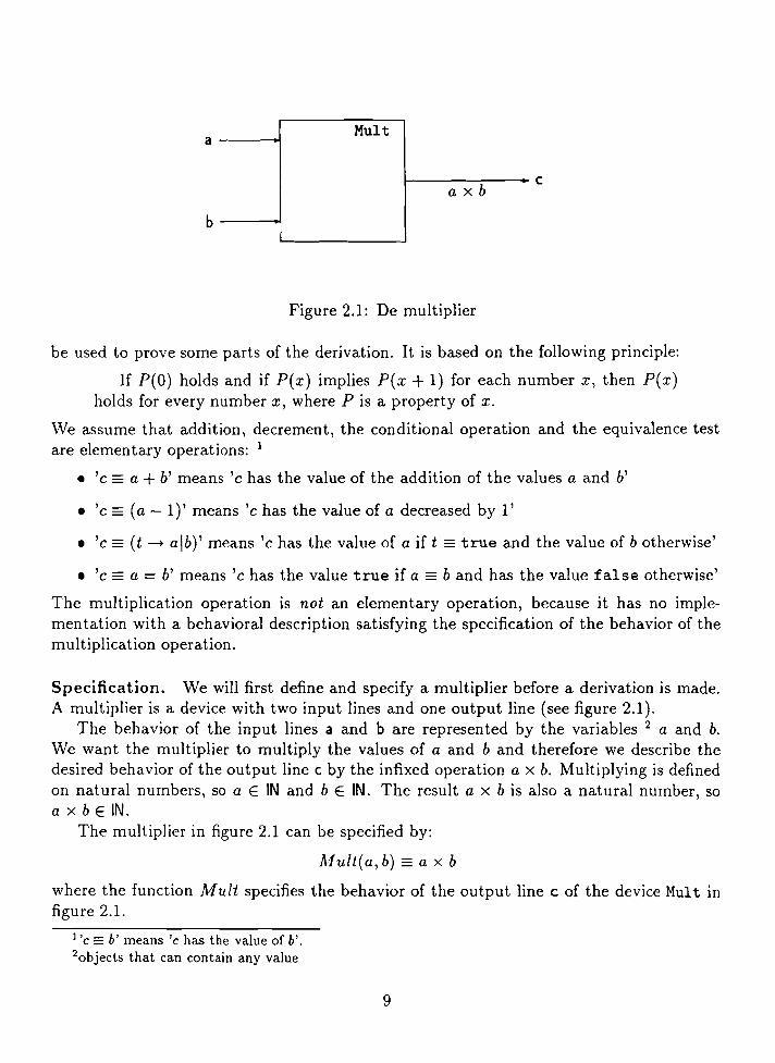
Multa -----I

1-----::---- Caxb

b--~

Figure 2.1: De multiplier

be used to prove some parts of the derivation. It is based on the following principle:

If P(O) holds and if P(x) implies P(x + 1) for each number x, then P(x)holds for every number x, where P is a property of x.

VVe assume that addition, decrement, the conditional operation and the equivalence testare elementary operations: 1

• 'e == a + b' means 'e has the value of the addition of the values a and b'

• 'e == (a - 1)' means 'e has the value of a decreased by l'

• 'e == (t --+ alb)' means 'e has the value of a if t == true and the value of b otherwise'

• 'e == a = b' means 'e has the value true if a _ b and has the value false otherwise'

The multiplication operation is not an elementary operation, because it has no implementation with a behavioral description satisfying the specification of the behavior of themultiplication operation.

Specification. We will first define and specify a multiplier before a derivation is made.A multiplier is a device with two input lines and one output line (see figure 2.1).

The behavior of the input lines a and b are represented by the variables 2 a and b.We want the multiplier to multiply the values of a and b and therefore we describe thedesired behavior of the output line c by the infixed operation a x b. Multiplying is definedon natural numbers, so a E IN and b E IN. The result a x b is also a natural number, soa x bE IN.

The multiplier in figure 2.1 can be specified by:

A1ult(a, b) == a X b

where the function Mult specifies the behavior of the output line c of the device Mult infigure 2.1.

J'c == b' means 'c has the value of b'.2 0 bjects that can contain any value

9

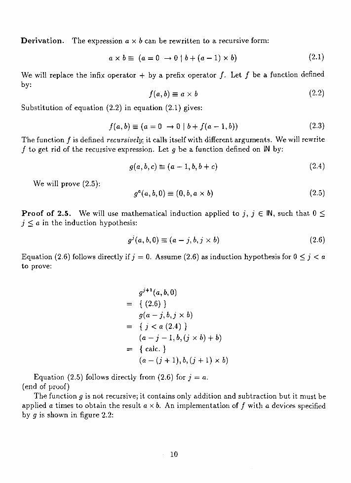
Derivation. The expression a x b can be rewritten to a recursive form:

a x b =(a = a -+ a I b+ (a - 1) x b) (2.1 )

We will replace the infix operator + by a prefix operator f. Let f be a function definedby:

f(a, b) = a x b

Substitution of equation (2.2) in equation (2.1) gives:

f(a, b) = (a = a -+ a I b+ f(a -l,b))

(2.2)

(2.3)

The function f is defined recursively; it calls itself with different arguments. We will rewritef to get rid of the recursive expression. Let 9 be a function defined on IN by:

We will prove (2.5):

g(a,b,c) - (a -l,b,b+ c)

gQ(a,b,O) _ (O,b,a x b)

(2.4)

(2.5)

Proof of 2.5. We will use mathematical induction applied to j, j E IN, such that a~j ~ a in the induction hypothesis:

gi(a,b,O) = (a-j,b,j x b) (2.6)

Equation (2.6) follows directly if j = O. Assume (2.6) as induction hypothesis for °~ j < a

to prove:

gi+ 1 (a,b,O)

{ (2.6) }

g(a -j,b,j x b)

{ j < a (2.4) }(a - j - 1, b, U x b) + b)

{ calc. }

(a - U+ l),b,U + 1) x b)

Equation (2.5) follows directly from (2.6) for j = a.(end of proof)

The function 9 is not recursive; it contains only addition and subtraction but it must beapplied a times to obtain the result a x b. An implementation of f with a devices specifiedby 9 is shown in figure 2.2:

10

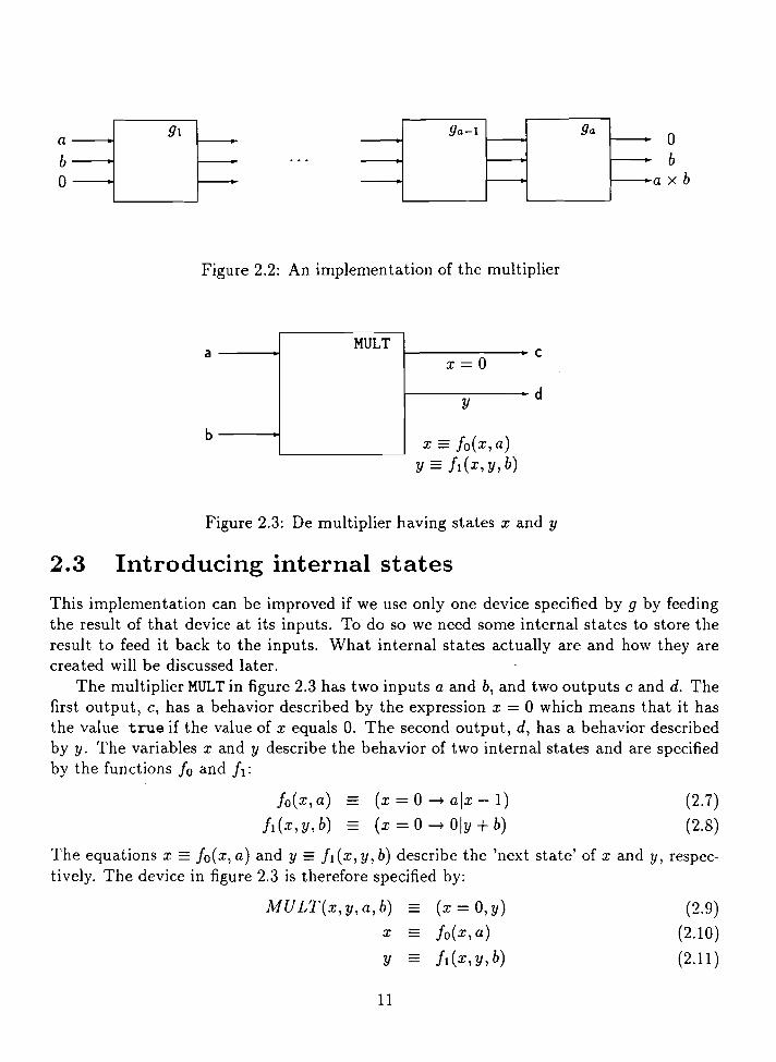
abo

91

Figure 2.2: An implementation of the multiplier

a

b

MULTx=O

Y

x == Io(x, a)

c

d

Figure 2.3: De multiplier having states x and y

2.3 Introducing internal states

This implementation can be improved if we use only one device specified by 9 by feedingthe result of that device at its inputs. To do so we need some internal states to store theresult to feed it back to the inputs. What internal states actually are and how they arecreated will be discussed later.

The multiplier MULT in figure 2.3 has two inputs a and b, and two outputs c and d. Thefirst output, c, has a behavior described by the expression x = 0 which means that it hasthe value true if the value of x equals O. The second output, d, has a behavior describedby y. The variables x and y describe the behavior of two internal states and are specifiedby the functions 10 and II:

Io(x,a) = (x = 0 -+ alx -1)

II (x, y, b) = (x = 0 -+ 0Iy + b)

(2.7)

(2.8)

The equations x == Io( x, a) and y == II (x, y , b) describe the 'next state' of x and y, respectively. The device in figure 2.3 is therefore specified by:

MULT(x,y,a,b) (x=O,y)

x == Io(x,a)

y - II (x, y, b)

11

(2.9)

(2.10)

(2.11)

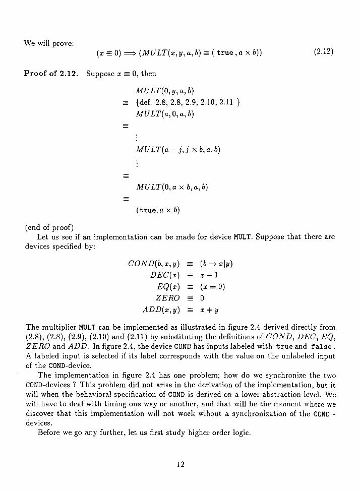
We will prove:(x =0) =} (MU LT(x, y, a, b) _ (true, a x b))

Proof of 2.12. Suppose x 0, then

MU LT(O, y, a, b){def. 2.8, 2.8, 2.9, 2.10, 2.11 }

.MULT(a, 0, a, b)

MULT(a - i,j x b, a, b)

MU LT(O, a x b, a, b)

(true, a x b)

(2.12)

(end of proof)Let us see if an implementation can be made for device MULT. Suppose that there are

devices specified by:

COND(b, x, y)DEC(x)

EQ(x)

ZERO

ADD(x,y)

(b---+xly)x-I

(x = 0)ox+y

The multiplier MULT can be implemented as illustrated in figure 2.4 derived directly from(2.8), (2.8), (2.9), (2.10) and (2.11) by substituting the definitions of COND, DEC, EQ,ZERO and ADD. In figure 2.4, the device COND has inputs labeled with true and false.A labeled input is selected if its label corresponds with the value on the unlabeled inputof the COND-device.

The implementation in figure 2.4 has one problem; how do we synchronize the twoCOND-devices ? This problem did not arise in the derivation of the implementation, but itwill when the behavioral specification of COND is derived on a lower abstraction level. Wewill have to deal with timing one way or another, and that will be the moment where wediscover that this implementation will not work wihout a synchronization of the COND devices.

Before we go any further, let us first study higher order logic.

12

d

c

r---------------,MULTI

X~I

ICOND EQ I

I IxI

~=OI Itrue --- I

I I~ false I~-1

IIIDEC

f-- II

IL...o.

CONDI

I

ZERO I

0true I

I.-- falseADD y

II f- II

fy+b

II II I

b

a

L ~

Figure 2.4: Implementation of MULT

13

Chapter 3

The description formalism

This chapter gives an introduction to typed higher-order predicate logic. It is not necessaryto read this section if you have some knowledge of higher order logic. However,it is the basisof the following chapters and can be helpful in understanding those sections. Especiallywhen types are discussed. This article was to a large extent inspired by [Pau87] and[Gor88].

3.1 Formal logic

A formal logic or calculus comprises assertions and inference rules. The assertions expressmeaningful statements that can be either true or false. An assertion is true if the statementexpressed by the assertion is true and it is false otherwise. Each inference rule has theform 'from A, B, ... conclude Q', where the assertions A, B, ... are the premises of therule, and Q is the conclusion. The theorems are those assertions that can be proved byapplying inference rules to other theorems. In order to have any theorems, there must beat least one axiom, a rule with no premises. A proofcan be written as a tree whose root isthe theorem, whose branches are rules, and whose leaves are axioms. An inference rule issound provided that if every premise is true, then so is the conclusion. A logic is sound ifall inference rules in it are sound. A logic is complete if every true assertion is a theorem(has a formal proof).

\Ve construct assertions from other assertions using logical connectives or quantifiers.For example, we can construct the assertion A 1\ B and the assertion A V B from theassertions A and B. The symbols V and 1\ are called logical connectives. The use of theselogical connectives is determined by inference rules.

3.2 First-order logic

In first-order logic and higher-order logic the assertions are called formulae. A formula isbuilt up from terms. In typed logic, every term has exactly one type. The use of typesimposes constraints on terms, but also makes a logic more complicated. We will therefore

14

study first-order logic and higher-order logic before types and typed terms are introduced.The terms in this section are untyped.

Functions. A function F is a set of ordered pairs such that, for each x in the domain ofF there is exactly one y in the range of F such that F(x) equals y. The domain of F is theset of all elements x such that F(x) exists. The range of F is the set of all elements y suchthat there is an x in the domain of F where y equals F(x). If F is a function and x is inits domain, then is F( x) a function application or combination. The function applicationF(x) is also written as (F x) .

n-place functions. An n-place function is a function F where each x in the domain ofF is an n-tuple. IF F is an n-place function, then we say that F has n arguments.

Variables. A variable is an object that can take any value. It can be replaced by anothervariable or a function application.

Terms. Terms denote mathematical entities such as sets, functions, or numbers. Weassume that there exists an infinite set of variables and, for each n ~ 0, a set of n-placefunction symbols. A term is a variable or a function application f(tl ... in), where f is ann-place function symbol and tt, . .. ,in are terms. A a-place function symbol is a constantsymbol; the term cO is written c and called a constant.

Predicates. A predicate is a formula: it can either be true or false. If P is an n-placepredicate symbol I and it, .. . ,in are terms, for any n where n ~ 0, then P(t l ••• t n) is apredicate. Predicates are also called atomic formulae. The a-place predicates are trueOand falseO; they are the only a-place predicates. They are written without parentheses:true and false abbreviates true() and false() respectively.

Formulae. A formula is a predicate or has the form (A), A 1\ B, A V B, A ==:::} B, ...,A,V'x.A or ::lx.A, where A and B are formulae and x is a variable.

The truth of non-atomic formulae is determined as follows:

• (A) is true if A is.

• A 1\ B is true if both A and B are. A formula constructed this way IS called aconjunction.

• A V B is true if either A or B is. A formula constructed this way is called a disjunction.

• A ==:::} B is true provided that if A is true then so is B. A formula constructed thisway is called an implication.

1 A predicate symbol that has n arguments.

15

• ...,A is true if A is false. A formula constructed this way is called a negation.

• Vx.A is true provided that A is true for every x. A formula constructed this way iscalled a universal quantification.

• 3x.A is true if A is true for some x. A formula constructed this way is called anexistential quantification.

The symbols A and B are formulae and x is a variable. The bi-implication A {:=? Babbreviates (A ==::} B)A(B ==::} A). Precedence conventions lessen the need for parenthesesin formulae. The symbol..., binds most tightly, followed by 1\, V, ==}, and ¢:::::} in decreasingorder. The scope of a quantifier extends as far to the right as possible. One quantifier canbind several occurrences of a variable at once. Example: Vx.A 1\ B V A 1\ C abbreviatesVx.((A A B) V (A 1\ C)). Binding and quantifiers will be defined later.

In [Gor86], Gordon uses the symbol J instead of ==:::} to denote implication. Althoughmany other articles have adopted the same symbol for implications, we will not do so.There is no reason to introduce a new symbol for denoting implications if the old one stillcan be used.

We will not discuss the axioms and inference rules [Pau87, p. 181-244] and assume a sufficient knowledge of predicate calculus. Textbooks about predicate calculus, like [End72],can be helpful.

3.2.1 Binding and substitution

We have discussed the logical connectives 1\, V, ==::::}, ..., and ¢::::::}. Together they arethe logical connectives of propositional calculus. Adding the universal quantifier and theexistential quantifier extends propositional calculus to predicate calculus, also called firstorder logic.

When expressing Vx.A, the formula A can contain a variable x. This is the case if A isa predicate with x as one of its arguments. In Vx.A, the variable x is said to be bound.

Sometimes renaming of a variable is necessary. If x and y range over natural numbersthen Vx.3y.x ¢ y is a true formula. 2 Substituting y for x, it is wrong to conclude 3y.y ¢ y.The problem is the capture of a free variable. The cure is to define what it means for avariable to occur free or bound in a term, and to restrict substitution accordingly.

Binding. A variable x occurs bound in a formula, defined by structural induction to itsoccurrence:

• x occurs bound in Vy.A or 3y.A if x and yare the same variable or x occurs boundin A

• x occurs bound in ...,A if x occurs bound in A

2The expression :I; == Y means ':I; equals y', :I; =$. y abbreviates -'(:1; == y).

16

• x occurs bound in A 1\ B, A VB, A ::::::::::} B, or A {::::::} B if x occurs bound in A or xoccurs bound in B

A variable x occurs free in a formula in the following cases:

• x occurs free in Vy.A or :3y.A if x and yare different variables and x occurs free in A

• x occurs free in ...,A if x occurs free in A

• x occurs free in A 1\ B, A VB, A ===::} B, or A {::::::::} B if x occurs free in A or x occursfree in B

• x occurs free in P( tt, ... ,tn) if x occurs in one of the terms t l , ... , tn, where P is ann-place predicate symbol.

Note that a variable can occur free as well as bound. For example, x occurs free in the leftdisjunct and bound in the right disjunct in:

x =0 V Vx.:3y.y < x

Substitution. We will express A[t/x] as the substitution of term t for the variable xin formula A. We can also express simultaneous substitutions: A[tI/Xl, ••• ,tn / Xn] is theformula that results from simultaneously substituting t l for Xl and ... and tn for X n inA. Substitution is also defined on terms: u[tI/X}, • •• ,tn / Xn) is the term that results fromsimultaneously substituting t l for Xl and ... and tn for X n in the term u.

In the substitution A[t/x]' the free variables of term t stand in danger of becomingbound in A. Substitution requires special care if a free variable of t occurs bound in A.Only free occurrences of x are replaced by t. If we want to define substitution correctlythen we have to rename bound variables of A if necessary to avoid the capture of a freevariable. Substitution can be precisely defined by induction on the structure of a formula:

• in Vy.A, if x equals y then the result of the substitution is Vy.A. Otherwise, if y occursnot free in t then the result is Vy.A[t/x]. Otherwise, let z be a variable different fromx and every variable occurring in A or t; the result is 'Iz.A[z/y][t/x].

• in :3y.A, substitution is similar to the previous case.

• in --.A, the result is --.(A[t/x))

• in A 1\ B the result is A[t/x] 1\ B[t/x]

• in A V B the result is A[t/x] V B[t/x]

• in A===::} B the result is A[t/x] ===::} B[t/x]

• in A {::::::::} B the result is A[t/x] ¢::::::? B[t/x]

• in P(UI, ... , urn), where P is an m-place predicate symbol and UI, ••. , Urn are terms,the result is P(Ul[t/X]' . .. , Urn [t/x]) , by substitution of the terms.

Renaming a bound variable is called a-conversion.

17

3.2.2 Quantification

The universal quantifier is defined by saying that a formula Vx.A is true if A is true forevery assignment of values to its free variables. So Vx.P(x) is true if P(x) is for all valuesof x, where P is an I-place predicate symbol.

The existential quantifier is defined by saying that a formula 3x.A is true if A is truefor at least one value of each of its free variables. So :Jx.P(x) is true if P(x) is for somevalue of x, where P is an I-place predicate symbol.

3.2.3 Mathematical Induction

Mathematical induction can be used to introduce a formula of the form Vx.A. An informalstatement of mathematical induction is:

Definition 1 (Mathematical induction) If P(O) is true and if P(x) implies P(x + 1)for every natural number x, then P(x) holds for every natural number x and predicate P.

3.3 Higher-order logic

By allowing quantification of predicate or function symbols we obtain second-order logic[End72, p. 268]. Allowing quantifiers over all formula variables gives higher-order logic[Pau87, p. 15]. Both formal logics imply the need for functions. It is necessary to studyterms and the equivalence or inequivalence between them before reasoning about functions.

3.3.1 Equality

Equality is expressed by the symbol =. The formula a == b denotes the equality betweentwo terms. 3 The symbol = is reserved for a test for the equality of two values resultingresulting in the boolean value true and false. Syntactically t = u is a term while t =uis a formula. 4

The equality predicate is an equivalence relation because it is reflexive, symmetric andtransitive.

3.3.2 Lambda expressions

A lambda expression or abstraction has the form: AX.t, where t is a term and x is a variable.It is defined by:

f == AX.t~ Vx·f(x) == t(x)

where f and t are functions.

3Bi-implication ¢:::::::> is defined on formulae, not on terms.4Gordon does not distinguish terms from formulae in [Gor88].

18

Currying For an n-place function h(XI, X2, . .. , x n ) it is possible to define H, for anyn ~ 1, by:

This representation is called currying, and H is a curried function.

Functionals A function that operates on other functions is called a functional or a higherorder function. The logic based on lambda expressions is called ..\-calculus.

Terms We have four kinds of terms: constants, variables, abstractions, and combinations.We did already discuss constants and variables. The abstraction (..\x.t), where t is a term,expresses the dependence of t upon x as a function. The combination (t u), where t and uare terms, denotes the application of the function t to the argument u.

We can omit brackets when the meaning is clear, writing P m n instead of ((P m)n) orP(m(n)). Also we can do a single..\ do the work of several, writing..\ x y.t instead of >.x.>.y.t.These conventions are especially convenient for curried functions: write (..\ x y.X2+y2) m ninstead of (((..\x.>.y.x2+ y2)m)n) or ((>.x ...\y.x2+ y2)(m))n.

3.3.3 Lambda reductions

Lambda reductions or conversions allow a term to be evaluated. Each reduction converts aterm to an equivalent term. Most important is f3-reduction, the substitution of a function'sargument into its body:

(>.x.t)u =t[u/x]

Another lambda reduction is the forming of combinations and abstractions:

r =81\ t =u ===} (r t) =(8 u)

t == u ===} (..\x.i) =(..\x.u)

Binding. Binding of variables by terms of the ..\-calculus can occur, so we must distinguish between free and bound variables. In >.x.t, the variable x is bound. Renaming thebound variable is called a-conversion:

..\x.t =..\y.i[y/x]

By a-conversion the formula f( x) == x2 means exactly the same as the formula f(y) == y2.The substitution of term t for variable x in term u, uri/x]' is defined inductively by

case analysis on u:

• u = >.y.r. If x equals y then uri/xl = ..\y.r. Otherwise, if y is not free in t thenu[t/x] - >.y.r[t/x]. Otherwise, let z be a variable different from x and every variableoccurring in r or t then u[t/x] = ..\z.r[z/y][t/x].

19

• U = (r s) <===> uri/xl == r[i/x](s[i/x]) .

• u is a constant or variable. If u equals x in uri/xl then uri/x] == ij otherwise uri/x] ==u.

The A-calculus is also described by Gordon [Gor79, p. 23-48] and [Pau87]. TypedA-calculus banishes many strange constructions that untyped A-calculus has. In typedA-calculus, each term belongs to one fixed type. Types can be constructed from the basictypes like' num " the type of natural numbers, or 'bool " the type of booleans. Types willbe defined in chapter 5.

20

Chapter 4

Specification

The example in section 2.2 has shown us how we can derive an implementation of a digitalcircuit when the behavior of that circuit is specified. Usually, we do not have the descriptionof the behavior of a device. Expressing the behavior of a device formally is a difficultprocess. Let us see how a behavioral description of a device is expressed.

4.1 A behavioral description

At the beginning of a design process, the digital engineer usually has an idea what hewants to design. His idea is also often not very concrete: he does not know what his designwill look like. He even does not know if his idea can be implemented. The first and mostdifficult problem for the engineer is writing down what he wants: the specification. Thespecification specifies the behavior of a circuit. It is usually expressed in the abstract andneeds working out.

The engineer starts with the specification. It specifies a 'black box' or 'device'; forexample:

This device is called 'Device' and has m input lines called al, ... ,am and n outputlines called bl, ... bn. The behavior of the output lines depends only on the digital signalsthat occur on the input lines. 1 The input lines aI, ... ,am are represented by variables

al,··· ,am'The behavior of the output lines bl, ... , bn is represented by the functions il,"" in

as shown above. The functions iI, ... ,in have the variables aI, ... ,am as arguments.The device Device can also be regarded as a function Device that has a domain with

m arguments and a range with n arguments. Figure 4.1 can be described by the followingfunction:

Device = A(a}, ... , am).(fl(al"'" am), f2(al"'" am), ... , in(a}, ... , am)) (4.1)

We usually make no difference between the name of an input line and the name of thecorresponding variable. The name of a device is usually also the same as the name of the

1 We will introduce 'states' in section 4.2

21

ai

a2

am

DeviceII(al, ... , am)

h(al, ... , am)

In (aI, ..• , am)

Figure 4.1: A device called Device

bi

b2

bn

corresponding function. However, input lines and devices are not variables and functionsrespectively.

4.2 Introduction of states

Sometimes, the engineer wants to use the concept of states in his design. We will discussstates in the context of structural abstraction. States are in fact the behavioral descriptionof internal lines that can not be expressed in the description of input lines. Let the followingexample explain this.

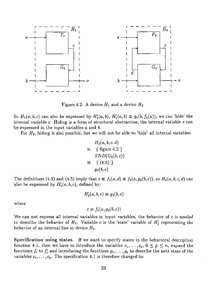
Suppose we have two devices HI and H2 • Device HI is constructed from FI and GI ,

and H2 is constructed from F2 and G2 (see figure 4.2). Let FI, F2 , GI and G2 be definedby:

FI - >'X.fI(X)F2 >'(x,y)·h(x,y)GI >'(X,Y)·91(X,y)

G2 >'(x'Y)'(92(X,Y),93(X,y))

where 11, !2, 91, 92, 93 are functions. Then we can derive

H1 (a,b,c)

{ figure 4.2 }

G1 (b,c)

{ (4.4) }

91 (b, c){ (4.2) }

91(b'!I(a))

22

(4.2)

(4.3)

(4.4)

(4.5)

o

r-------,H2I F2

II

I Ic

I ,.. f0o- I

I I

I I

I G2I

I '----- -- I

Id

I

b

a

o

r - - - - - - ill 'I

F1II

I Ic

I r-- I

I I

I I

I GII

I -- I

I I

I Ib

a

L J L J

Figure 4.2: A device HI and a device H2

So H1(a,b,c) can also be expressed by H~(a,b), H~(a,b) =9l(b,fI(a))j we can 'hide' theinternal variable c. Hiding is a form of structural abstraction; the internal variable c canbe expressed in the input variables a and b.

For H 2 , hiding is also possible, but we will not be able to 'hide' all internal variables:

H2 (a,b,c,d){ figure 4.2 }

SND(G2 (b,c))

{ (4.5) }

93(b,c)

The definitions (4.3) and (4.5) imply that c =!2(a,d) =!2(a,92(b,c)), so H2(a,b,c,d) canalso be expressed by HHa, b, c), defined by:

H~(a,b,c) =93(b,c)

where

We can not express all internal variables in input variables; the behavior of c is neededto describe the behavior of H2 • Variable c is the 'state' variable of H~ representing thebehavior of an internal line in device H 2 •

Specification using states. If we want to specify states in the behavioral descriptionfunction 4.1, then we have to introduce the variables Cl,'" ,Cp , 0 ~ p ~ n, expand thefunctions Ii to II and introducing the functions 91, ... ,9p to describe the next state of thevariables CI, .•. , cpo The specification 4.1 is therefore changed to:

23

Device =A(al"'" am, Cl, ... , Cp ).

(f~ (a l, ... , am, Ct, , Cp),

f~(al"'" am, Cl, , cp ),

where Cl, ... , Cp are internal variables defined by:

Cl - 9l(at, ,am ,cl'''''Cp )

C2 - 92(al, ,am,ct, ... ,cp )

4.3 Transformation and decomposition

How can we derive a circuit from its specification ? Basically, deriving can be done by

1. Calculating a functional description from the specification towards the specificationsof implemented circuits. This is called decomposition. We have seen a decompositionin the example of the multiplier (see section 2.2).

2. Rewriting the expression of variables and functions that occur in the specification.This is called transformation. For example, the rewriting of variables expressed innatural numbers, IN, to variables and functions expressed in the boolean values, IB,is a transformation.

Figure 4.3 illustrates the transformation of a function F, defined on u, to F', definedon T. The function c.p converts a variable expressed in u to a variable or function expressedin T. The function 1r is the inverse function of c.p; it converts from T back to u.

Transformation can be useful because it is sometimes not possible to decompose afunction without transforming it first. For example, there is not much left to decomposeon a + b, where a and b are in IN. By transforming a and b to IB*, a + b can be decomposedto a functional description of an implementation. 2

Deriving specifications by transformation is based on types. We will discuss this kindof derivation after we have studied the types and typed terms in higher-order logic.

21S· abbreviates the Cartesian product IB x ... x lB.

24

Fa

TF'

T

Figure 4.3: Transformation from a to T

25

Chapter 5

Types and typed terms

In a typed logic each term has one fixed type. Each type T denotes a set D(T). The set D(T)contains special terms with a unique name denoting a fixed value. For example the typeboo I has the set D( bool) containing the terms true and false. We call such termsconstants.

A type T consists of all constants having type T, all contained in the set D(T).The expression 't has type T' is written as t : T. Each term has to have a type, so any

expression using a term t must indicate the type of t. For example, we must write the typeT of variable x in \Ix : T.t, because we do not know the type of x if T is omitted. The typeof t does not need to be explained; t is a formula, because \I is defined on formulae.

Sets and types. Sets can also be used instead of types. By replacing each type T byD(T) and replacing each expression t : T by t E D(T), we can omit types. We haveintroduced types because sets are already used as terms. By using types instead of setsthere can be no confusion between sets used as terms and sets used instead of types. Asimilar distinction is made between formulae and bool-typed terms.

5.1 Partial ordering

If each type (7 contains a special constant l.q, then the concept of partial ordering can beused. 1 If t : (7.t = l.q, then t is said to be undefined.

Any type (7 containing l.q has a partial ordering (D((7), ~q), where \Ix : (7 .l.q ~ x.The formula x ~q y means that x is less then y in that partial ordering. We say that xapproximates y.

Approximation. Approximation is reflexive, anti-symmetric and transitive. It can beextended to functions:

\If g. (\lx.f x ~ 9 x) ::::::? f ~ 9

ISee [Pau87, p. 61].

26

Approximation can be used to express functions partially. For example, assume that f and9 are functions. Let al and a2 be constants in the domain of both functions, and bl andb2 be constants in the range of both functions. Suppose that we know that f( ad == bl istrue. Vle can define f, for all x such that x t= all by:

f(x) = 1..

Suppose that we know more about g: g(at} _ bl and g(a2) == b2, then is 9 defined by, forall x such that x t= al and x t= a2:

g(x) == 1..

The extension of approximation to functions allows us to conclude:

fr;,g

\Ve say that function 9 is stronger than f.Approximation can be used to define equality:

Vt u.(t r;, u 1\ u r;, t) {:::=} t =u

The conversion rules for equality, described below, also apply for approximation.Partial ordering is the basis of many useful properties like structural induction [Pau87,

p. 125] which will not be explained here. We will however use the partial ordering r;,u for atype (Y to express a evaluation of two terms, usually functions, that are not equal. We wantto do this, because it gives the possibility to reason about different functions describingthe operation of a single digital circuit.

5.2 Type operators

Let us study the four kinds of types:

1. Type variables

A type variable can be regarded as a type where the specific form of that type is notyet known. It can be substituted by any other kind of type, even if the type variablecontains other type variables after substitution. Types containing type variables arecalled polymorphic; others are monomorphic.

2. Type constants

These have names like boolor num. They denote fixed sets of values. Every constanthas a type constant as its type. They all have unique names; not one constant hasthe same name as another constant having the same type.

27

3. Function types

If 0'"1 and 0'"2 are types, then 0'"1 -+ 0'"2 is the type of all functions with domain 0'1 andrange 0'2; it denotes the set of functions from the set denoted by its domain to theset denoted by its range.

4. Compound types

These have the form (0'1, ••• ,O'n)op, where the types 0'1, ••• ,O'n are the argumenttypes and op is a type operator of arity n.

Type operators. A type operator is identified by a pair (op, n), where op is the name ofthe type operator and n is its arity. It is defined by constructor functions and destructorfunctions or an eliminator junctional 2. The set Tyops is the set of type operators.

Instances of a type. An instance 0'"' of a type 0' is obtained by replacing all occurrencesof a type variable in 0' by monomorphic types. The only instance of a monomorphic typeis the type itself.

Notation of types. Compound types are written in postfixed form to distinguish thedifference between compound types and function applications.

The set Tyvars is the set of type variables. Type variables are usually denoted by smallGreek letters. The type of a bound variable is sometimes left out instead of writing downa small Greek letter. For example: write AX : 0'. t as AX. t.

Type constants and constants are denoted by letters in the typewriter font or bynumbers.

Expression in compound types. Function types and type constants can be expressedas compound types. A function type is a compound type with type operator (-+,2). Weusually write 2-ary type operators in the infixed form instead of the postfixed form:

• Function types are written as 0'1 -+ 0'"2 instead of (0'1, 0'"2) -+

• Disjoint union types are written as 0'1 + 0'"2 instead of (0'1,0'2)+

• Cartesian Product types are written as 0'1 x 0'2 instead of (0'1'0'2)X

Writing AX : T.t indicates the type of the bound variable x. The function-type operatorassociates to the right: 0' -+ (T -+ v) is abbreviated 0'" -+ T -+ v. The product-typeoperator associates to the right, too.

A type constant is a compound type built with O-ary type operators. For example, thetype constant num is expressed as the compound type 0 num. It is therefore sufficient todefine the set of types as type variables and compound types. The set Types of types isthe smallest set such that:

2See page 29.

28

• Tyvars ~ Types.

• If O'j E Types, for all i : 1 ~ i ~ n, and (op, n) E Tyops, then (0'1 ..• O'n)OP E Types.

• If 0' E Types and u' is an instance of 0', then 0" E Types.

Note that Tyops must contain at least one O-ary type-operator; otherwise no monomorphic types can be constructed. We will assume that the 2-ary function type, the 2-aryproduct type and the 2-ary union type are available; (2, -+), (2, x) and (2, +) are elementsof Tyops.

5.3 The basic types

Basic types are the type constants that will be used here. We already mentioned' num 'as the type of the natural numbers 0,1, ... , and' bool ' as the type of the boolean valuestrue and false. All terms having type bool can either be true or false. The typeconstants num and bool can be expressed as the compound types 0 bool and 0 num 3;(num,O) and (bool ,0) are elements of Tyops.

5.4 The Cartesian product type

Types can be constructed from basic types by using constructor functions for creatingelements of the type. For taking elements apart it may have destructor functions or else aneliminator functional. The Cartesian product type u x T, can be constructed using threeconstant symbols:

PAIR

FST

SND

0' -+ T -+ (u X T)

(0' X T) -+ 0'

(0' X T) -+ T

The ordered pair (t, u) is an abbreviation for PAlR(t)(u). For x 0' and y T, the pair(x,y) has type 0' x To

The axioms areFST(x,y) = x

SND(x,y) = y

(FST z, S N D z) = z

The third axiom, sometimes called surjective pairing, asserts that every member of u x T

has the form (x, y) for unique x : 0' and y : T. Equivalent is the exhaustion axiom

Vz: u x T.3x: O',Y: T.Z =(x,y)

3See page 28

29

The surjective pairing axiom implies the exhaustion axiom, putting F ST( z) for x andSND(z) for y. Exhaustion implies surjective pairing: it allows the replacement of z by(x,y), reducing (FSTz,SNDz) == z to

(FST(x,y),SND(x,y)) =(x,y)

5.5 The disjoint union type

The disjoint union type + has three constant symbols:

INL

INR

WHEN

0'-+(0'+7")

7" -+ (0' + 7")

(0' -+ v) -+ (7" -+ v) -+ (0' + 7") -+ V

INL and INR are constructor functions, WHEN is an eliminator functional. For x : 0',y : 7", f : 0' -+ v and g: 7" -+ v, the reduction axioms for WHEN are

WHEN(J)(g)(INLx) =f(x)

WHEN(J)(g)(INRy) = g(y)

The exhaustion axiom asserts that an element of type 0' + 7" has the form INL(x) orIN R(y) for x : 0' and y : 7". It is

vz: 0' + 7" • (3x : 0'. Z = INLx) V (3y : 7". z = INR y)

It implies WHEN(INL)(INR)(z) =z.

5.6 Typed terms

We can define the set Terms of terms formally. Each term is a pair (c, 0'), where c is thename of the term and 0' is its type. Let Consts be the set of all constants, that is all termshaving a unique name and a type-constant as their type. The name of every constanthaving type 0' occurs as an element of D(O'). The set Terms is the smallest set such that:

• If x is a name which is not the name of a constant, and 0' E Types, then (x,O') ETerms. Terms formed in this way are called variables.

• If (c, 0') E Consts and 0" E Types is an instance of 0', then (c, 0") E Terms. Termsformed in this way are called constants.

• If (t, 0" -+ 0') E Terms and (t',O") E Terms then ((t t'),O') E Terms. Terms formedthis way are called combinations or function applications.

30

• If (x,a) E Terms (where x is the name that is not the name of a constant) and(t, a') E Terms and a -+ a' E Types then ((Ax: a. t), a -+ a') E Terms. Termsformed this way are called abstractions or A-terms.

The instantiation of terms is defined as the replacement of variables in a formula byterms with the same type.

5.7 The bool - type

The type bool has the operator symbols having a similar meaning as the operator symbolsfor formulas. We will use the same symbols as we have done for formulas:

• the term a 1\ b: bool has the value true if term a : bool and term b: bool havethe value true

• the term a vb: bool has the value true if term a : bool or term b: bool havethe value true

• the term ...,a: bool has the value true if term a : bool has the value false

The set Consts contains at least (1\, (bool x bool) -+ bool), (V, (bool x bool) -+

bool ), (..." bool -+ bool), ( true, bool ) and ( false, bool). The choice for the symbols 1\, V and..., can be confusing because the same symbols are used as logical connectives.The context in which we use them is usually clear enough to determine if we are using thelogical connectives or the booloperators. The constants true and false are written inthe typewriter font while the logical atomic symbols true and false are written in italics.We sometimes write the term 't == true', for a term t : bool, simply as 't' to makeformulae shorter. We sometimes write '...,t' instead of 't = false' for the same reason.

The conditional operator uses the bool - type to choose between two terms having thesame type. It has type (bool x a x a) -+ a and is defined by

(p -+ tlu)

meaning that if p is true then the result is t else it is u. Note that p has a boolean value.We use the symbol -+ although the same symbol is used for denoting function types. Thiswill not cause any confusion; the symbol -+ expresses function types if it occurs in a typeexpression and it expresses a conditional if it occurs in a term or a formula.

Formally, the conditional operator is the function COND : (bool x a x a) -+ a, where(p -+ tlu) abbreviates COND(p,t,u). It is a constant; (COND,( bool x a x a) -+ a) EConsts.

The equality operator '=' gives a bool - typed term as result. It is an infixed functionhaving type (a x a) -+ bool and is defined by

'Vtu.(t =u) ¢::::::> ((t = u) =true)

Note the difference between =, = and ¢:::=}:

31

'{=:::::}' has formulas as arguments and results in a formula

'='

'-'

has terms as arguments and results in a formula

has terms as arguments and results in a bool - typed term

The equality operator is a constant: (=, (0" X 0") -+ beol) is an element of Consts.The equality operator can be used for boel - typed arguments with the following the

orem:Vt,u: bool. ((t 1\ u) V --.(t V u)) = (t = u)

Note that we use the beol-typed operators 1\ and V. The result is a bool term.The equality operator can be used for num -typed arguments with the following theorem:

Vt,u: num. ((t ~ u) 1\ (u ~ t)) == (t = u)

5.8 The num - type

The num type has operators for addition (+), multiplying (x) and subtraction (-) thatwill result in a term. They all have the type (nwn x num) -+ num and can be regardedas infixed functions. We will not define these functions here.

There are also operators for comparing two numbers. For example, the less-then-orequal-to operator (~), the greater-then-or-equal-to operator (~), the less-then operator«) and the greater-then operator (». They all have type (num x num) -+ beel andare infixed functions, too. The result is a term having the boolean value true or false.

The example in the next section makes use of the modulo operator, 'mod " and thedivision operator, 'div '. They can be defined as follows (z, a, b: num):

(z =a mod b) {::::::} (3n : num .(z =a - n x b) 1\ (0 ~ a - n x b < b))

a = b x (a div b) + a mod b

Both 'div ' and 'mod' are infixed functions having type (num x num) -+ num. All theoperators mentioned above must, together with their types, occur in the set Consts.

32

Chapter 6

Transformation

In section 4.3, we expressed transformation as a form of abstraction. Transformation can beregarded as the 'translation' of a function, defined on a type, to another function, definedon a different type such that both functions specify the behavior of a device in exactly thesame way.

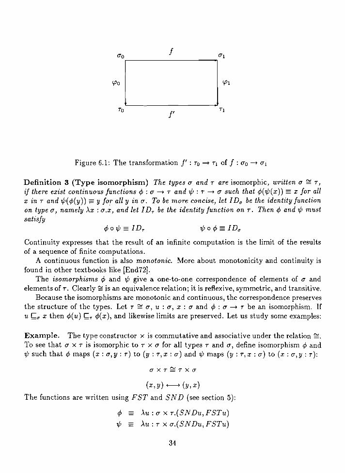
A formal definition is illustrated by figure 6.1 and defined by:

Definition 2 (Transformation) A function I' : To -+ T} is a transformation of a function f : 0"0 -+ 0"1 if there exists a function "Po : 0"0 -+ To and a function "PI : 0"1 -+ Tl suchthat, for all x : 0"0:

l'("Po( x)) == "PI (J( x))

The concept of transformation is useful to express abstraction of specifications or functional descriptions. For example, let f : (num x num) -+ num be a function specifying adevice that adds its input values:

I(a,b)=a+b

Let 'byte' be a type representing values that can occur on some digital lines. Supposethat there are various digital circuits implemented, then those circuits can be specified withfunctions defined on byte. If the function l' : (byte x byte) -+ byte is a transformationof I, expressed in functions specifying implemented circuits, then I' and therefore f canbe implemented. We do not have to look at l' once its implementation is found, becauseI specifies the same implementation on num instead of byte. We can use I to deriveimplementations of other devices specified in num without looking at 1'.

\Ve will derive some useful properties of transformation.

6.1 Type isomorphism

We have discussed types in section 5. The isomorphism between types can be used infinding a transformation of a function to another. The definition of type isomorphism isextracted from [Pau87, p. 80, 81]:

33

0'0 f 0'1.------------..,

<po

10l'

<PI

Figure 6.1: The transformation f' : 10 - II of f : 0'0 - 0'1

Definition 3 (Type isomorphism) The types 0' and I are isomorphic, written 0' ~ I,

if there exist continuous functions 4> : 0' - I and'l/J : I - 0' such that 4>('l/J(x)) == x for allx in I and 'l/J( 4>(y)) == y fO,r all y in 0'. To be more concise, let I D I1 be the identity functionon type 0', namely AX : O'.X, and let I D-r be the identity function on I. Then 4> and 'l/J mustsatisfy

4> 0 'l/J =1D-r

Continuity expresses that the result of an infinite computation is the limit of the resultsof a sequence of finite computations.

A continuous function is also monotonic. More about monotonicity and continuity isfound in other textbooks like [End72].

The isomorphisms 4> and 'l/J give a one-to-one correspondence of elements of 0' andelements of 1". Clearly ~ is an equivalence relation; it is reflexive, symmetric, and transitive.

Because the isomorphisms are monotonic and continuous, the correspondence preservesthe structure of the types. Let I ~ 0', U : 0', X : 0' and 4> : 0' - I be an isomorphism. Ifu ~11 x then 4>(u) ~-r 4>(x), and likewise limits are preserved. Let us study some examples:

Example. The type constructor x is commutative and associative under the relation ~.

To see that 0' x I is isomorphic to I x 0' for all types I and 0', define isomorphism 4> and'l/J such that 4> maps (x: O',y: I) to (y : I,X: 0') and 'l/J maps (y : I,X : 0') to (x: O',y: I):

O'XI~IXO'

(X, y) +----7 (y, x)

The functions are written using FST and SND (see section 5):

4> AU : 0' x I.(SNDu, FSTu)

'l/J AU : I X O'.(SNDu, FSTu)

34

So the only thing that <p and 'IjJ do is swapping elements.The following isomorphism also holds:

The corresponding isomorphisms are easy to construct (see [Pau87, p. 81]). We cangeneralize this to the n-place product type. Let t1 : 0'1, ... , t n : O'n be terms. Then(t 1, ... , tn) abbreviates (i 1, (... , (tn-I, t n) .. .)). Its type is 0'1 X ... X O'n, which abbreviates0'1 x (... x (O'n-1 X O'n)" .). If 0'1, ... , O'n are all equal to a type 0', we write (O')n whichabbreviates 0' x ... x 0' X 0'

Another isomorphism

which expresses the distribution of function types over product types. It will be used insection 8.2 to prove signals isomorphic.

6.2 Transformation as type isomorphism

\Ve can prove the existence of an implementation of any function by proving an isomorphism between the types of the function and the types of functions specifying implementedcircuits, for example type byte. To do this, theorem 1 is required:

Theorem 1 (Isomorphic transformation theorem) For each function f 0'0 -+ 0'1the1'e exists a transformation f' : 'To -+ 'T1 if

Proof Because 0'0 ~ 'To, there exists an isomorphism function rp : 0'0 -+ 'To and because0'1 ~ 'T1 there exists an isomorphism 'IjJ : 0'1 -+ 'T1 (see figure 6.2). Define a functionf' : 'To -+ 'T1 by:

(6.1 )

then f' is a transformation of f, because, for all x in 0'0:

!,(rp(x)) == 'IjJ(f(rp-1(rp(X)))) == 1jJ(f(x))

(end of proof)Looking at the byte type, we can try to prove that any function defined in nwn has a

transformation defined in byte if we can proof that nwn and byte are isomorphic. Thiswill be difficult, because D( nwn) is infinite while byte is finite; byte represents a fixednumber of digital lines each accepting only two values (L and H). However, we can proveisomorphism between a type denoting a finite subset of nwn and byte provided that bytecan handle enough values. We will study this in the next section.

35

TO

r,p-l

I

I'

l/J-l

Figure 6.2: Transformation of I to f' using type isomorphism

6.3 Types for subsets of D(num)

We will define the type numm for all m ~ 0 where:

D(numm) = {0,1, ... ,2m -I}

so D(nUInm) C IN. Type numm has the following infixed operators:

EBm (numm x numm) --+ numm®m (numm x nUInm) --+ nUInm8m (numm x numm) --+ numm

They express addition, multiplication and subtraction in numm , respectively. The definitions are, for a and b in nwnm :

a EBm b

a®m b

a 8m b

(a+b)mod2m

_ (a x b) mod 2m

(a - b) mod 2m

So (numm, 0), (®m, 2), (EBm, 2) and (8m, 2) are in Tyaps. We usually leave out the subscriptof each operator symbol when the types of the arguments indicate its value. We will provethat nwnm and (nurnl)m are isomorphic.

Theorem 2

36

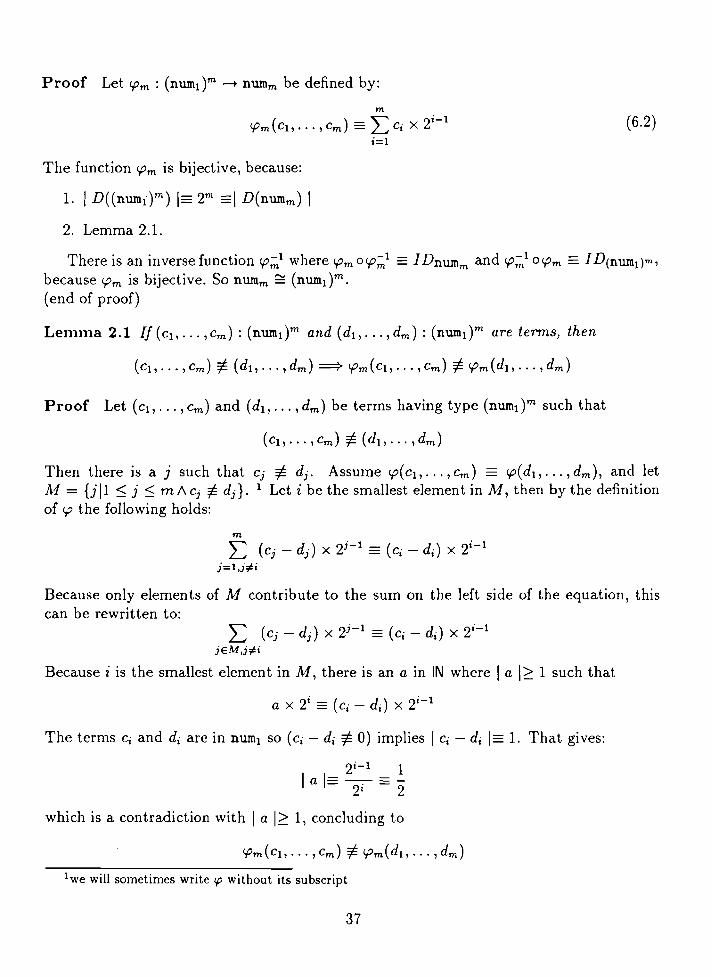
Proof Let 'Pm : (numdm --t numm be defined by:

m

( ) - " 2i-

1'Pm C1,···, em = L..J Ci X

i=l

The function 'Pm is bijective, because:

2. Lemma 2.1.

(6.2)

There is an inverse function 'P;;./ where 'Pm o'P;l == 1Dnumm and 'P;1 o'Pm == I D(num1)m,because 'Pm is bijective. So numm ~ (numdm.(end of proof)

Lemma 2.1 If (C1' ... ,cm ) : (num1)m and (d1 , • •• , dm ) : (num1)m are terms) then

(C1 , ... , cm ) ¢ (d1, ... , dm ) ==} 'Pm (C1, ..• , Cm) ¢ 'Pm (d1, ... , dm )

Proof Let (C1,' •• ,em) and (db" . ,dm ) be terms having type (num1)m such that

Then there is a j such that Cj ¢ dj • Assume 'P(C1, ••• , cm ) 'P(d1 , ••• , dm ), and let11.1 = {j 11 ~ j ~ m /\ Cj t=- dj }. 1 Let i be the smallest element in M, then by the definitionof 'P the following holds:

m

L (Cj - dj ) X 2j-

1 =(Cj - dj ) X 2i-

1

j=1.jeFi

Because only elements of M contribute to the sum on the left side of the equation, thiscan be rewritten to:

L (Cj - dj ) X 2j-

1 = (Ci - dd X 2i-

1

jEM,jeFi

Because i is the smallest element in M, there is an a in IN where Ia I;::: 1 such that

a x 2i == (Ci - d i ) X 2i-

1

The terms Ci and di are in num1 so (Ci - di ¢ 0) implies ICi - di 1_ 1. That gives:

2i - 1 1I a 1= 2i == 2

which is a contradiction with I a I;::: 1, concluding to

lwe will sometimes write tp without its subscript

37

(end of proof)We are interested in r.p~1, because we will use it in the derivation of an adder defined

on numm . Let 1r : (num X numm ) -+ numb for 1 Sis m and n : numm be defined by:

1r(1, n) == (n div 21-

1) mod 2

Then theorem 3 holds:

Theorem 3

r.p;;/(n) = (1r(l,n), ... ,1r(m,n))

Proof The following equation for 1 SiS m and n, n : numm , is true:

Then we can derive:

r.pm(1r(l, n), ... ,1r(m, n))

m

L2i- 1 x (ndiv2 i - 1 ) _2i x (ndiv2i)

i=1

This results in n because n is in D(numm ). So

r.p~1 =(1r(l,n), ... ,1r(m,n))

(end of proof)

6.4 Implementations

(6.3)

Implementation types are types that can be used to specify basic digital components, likeNAND-gates, NOR-gates or inverters directly. They are types that can only specify thevalues that are determined on a digital line (L and H) or the types that can be constructedwith the product type operator from other implementation types.

There must be just enough operations on these types to specify the basic digital circuitssuch that any function defined on implementation types can be implemented.

An example of an implementation type is numl; its constants 0 and 1 specify the valuesthat are determined on a digital line. The operation a EBI b represents the behavior of the

38

XOR-gate2 with inputs a and b. Similarly, a@l b represents the AND-gate. We do not haveto have an operation for all basic digital circuits; type numl has no operations for specifyingthe OR-gate and the inverter. There is no need to define new operations because the ORgate and the inverter can be expressed in AND-gates and XOR-gates. By case analysis wecan see that for any specification by 1-ary and 2-ary functions on implementation typesthere is decomposition possible using the constants 0 and 1 and EIh and @l as operators.

Let us define the functions that specify digital circuits:

Definition 4 (Implementation function) A function f : a -+ T specifies an implementation if it is expressed in operations on a and T and if a and T are implementationtypes.

We call a function specifying an implementation an implementation function.There are also functions defined on abstract types. Abstract types are types other than

implementation types. Some of those functions can be implemented:

Definition 5 (Implementable function) A function f : a - T can be implemented ifthere exists a transformation f' : a' - T ' such that f' is an implementation function.

The following theorem can be proved:

Theorem 4 A ny function f : a - T can be implemented if its types a and T are isomorphic to implementation types.

Proof Let a' and T ' be implementation types such that a' ~ a and T ' ~ T. Thenthe isomorphic transformation theorem, theorem 1, states that there is a transformationf' : (7' - T' of f. Any function defined on implementation types can can be implementedand therefore be expressed in operations of these types, so f' is an implementation function.(end of proof)

6.5 The adder

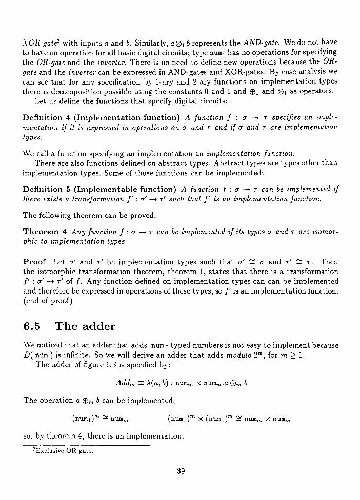
\Ve noticed that an adder that adds num - typed numbers is not easy to implement becauseD( num ) is infinite. So we will derive an adder that adds modulo 2m

, for m 2:: 1.The adder of figure 6.3 is specified by:

Addm =.A(a, b) : numm x numm.a EBm b

The operation a EBm b can be implemented;

so, by theorem 4, there is an implementation.

2Exclusive OR gate.

39

a -----I

1-----;,----- suma EBm b

b -----+I

Figure 6.3: The adder Addm

x

Y

C1

Addl

f(x,y,CI)

g(x,y,CI)

Figure 6.4: The one-bit full adder Addl

sum

co

Which one? Let us call the implementation function F:" : ((numdm x (numl)m) -+

(numdm. Vie can find it directly with equation 6.1 because both 'fi and ep-l are known (seedefinitions 6.2, 6.3 and theorem 3):

F:n =>'x y: (numdm.ep-l(ep(x) EBmep(y)) (6.4)

The decomposition of this function is not so easy. However, it can be decomposed. We willdecompose Fm : ((numdm x (numt)m x numd -+ (numdm using one-bit full adders (figure6.4) where f : (numd3 -+ numl and 9 : (numd3 --+ numl defined by:

f - >'(x,y,z): (numl?'X EBI Y 811 z9 = >'(x,y,z): (numd3 .(x 01 y) EBI (x 01 z) EBI (y 01 z)

It can be derived that:

f == >.(x, y, z) : (numl)3.(x + Y + z) mod 2

9 = >.(x, y, z) : (numl)3.(x +Y + z) div 2

(6.5)(6.6)

(6.7)(6.8)

We can implement Fm +l using m + lone-bit full adders as illustrated by figure 6.5.The specification of Fm is, for (Xl, ... , xm) : (numdm, (Yh' .. , Ym) : (numdm and C : numl:

Fm((Xl,' ",Xm),(Yl,···,Ym),C) ==(J(Xl, Yl, C), f(X2, Y2, g(Xl, Yl, C)), ...

. . . ,j(xm,Ym, g(Xm-l, Ym-I, g( . .. , g(Xl, Yl, C) ...)))

40

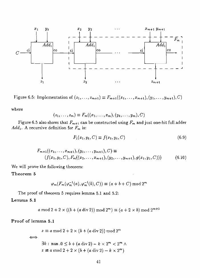
CCl

Xl Yl

co

r

I

I .C1

L

co Cl

Xm+l Ym+l

co

Figure 6.5: Implementation of (Zll"" Zm+d - Fm+1((Xl"" ,Xm+l), (Yl,'" I Ym+d, C)

where(Zl"'" Zm) = Fm((XI, ... , Xm), (Yl"'" Ym), C)

Figure 6.5 also shows that Fm +l can be constructed using Fm and just one-bit full adderAdd1 . A recursive definition for Fm is:

Fm+l((Xl, ... , Xm+l), (Yl," . I Ym+l), C) =(J(Xl' YI, C), Fm((X21 .•• I xm+d, (Y2, . .. I Ym+d, g(Xl, yI, C)))

We will prove the following theorem:

Theorem 5

The proof of theorem 5 requires lemma 5.1 and 5.2:

Lemma 5.1

a mod 2 +2 x ((b + (a div 2)) mod 2m) = (a + 2 x b) mod 2m +1

Proof of lemma 5.1

Z =a mod 2 + 2 x (b + (a div 2)) mod 2m

3k : num.O :S b+ (a div 2) - k x 2m < 2m A

Z =a mod 2 + 2 x (b + (a div 2) - k x 2m)

41

(6.9)

(6.10)

3k : num.l ~ 1 + b+ (a div 2) - k x 2m~ 2m 1\

Z =a +2 x b - k x 2m +1

3k : num.2 ~ 2 + 2 x b+ 2 x (a div 2) - k x 2m+! ~ 2m

+! 1\

Z _ a + 2 x b - k x 2m +1

===> {O ~ a mod 2 < 2 }

3k: num.O ~ a mod 2 +2 x b+ 2 x (a div 2) - k x 2m +1 < 2m +1 1\

z - a +2 x b - k x 2m +1

z = (a+2 x b) mod 2m +1

(end of proof)

Lemma 5.2 If'~~l(a) == ((amod2),<p~1(adiv2))

Proof of lemma 5.2 We can derive 11"(1, a) =a mod 2 and, for 1> 1

11"(1, a)

((a div 21- 1) mod 2)

(((a div 2) div 21-

2) mod 2)

11"(/- 1, a div 2)

Using theorem 3 gives

(11"(1, a), 11"(2, a), ... , 1I"(m + 1, a))

(a mod 2, (11"(1, a div 2), ... , 1I"(m, a div 2)))

(a mod 2,<p;;-/(a div 2))

(end of proof)

42

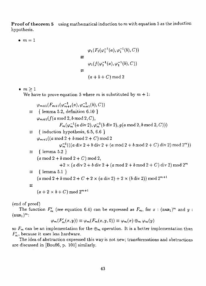
Proof of theorem 5 using mathematical induction to m with equation 5 as the inductionhypothesis.

e m= 1

(a + b+ C) mod 2

em2::1\Ve have to prove equation 5 where m is substituted by m + 1:

'Pm+! (Fm+1('P~~1 (a), 'P~~1 (b), C)){ lemma 5.2, definition 6.10 }

'Pm+l (I(a mod 2, bmod 2, C),Fm('P~1 (a div 2), 'P~/(bdiv 2), g(a mod 2, b mod 2, C)))

{ induction hypothesis, 6.5, 6.6 }

'Pm+! ((a mod 2 + bmod 2 + C) mod 2

'P~l(((a div 2 + b div 2 + (a mod 2 + b mod 2 + C) div 2) mod 2m))

{ lemma 5.2 }

(a mod 2 + b mod 2 + C) mod 2,

+2 x (a div 2 + b div 2 + (a mod 2 + bmod 2 + C) div 2) mod 2m

{ lemma 5.1 }

(a mod 2 + bmod 2 + C + 2 x (a div2) + 2 x (bdiv 2)) mod 2m +1

(a + 2 x b+C) mod 2m +1

(end of proof)The function F:n (see equation 6.4) can be expressed as Fm , for x : (nwndffi and y :

(nwn l )m:

so Fm can be an implementation for the EBm operation. It is a better implementation thanF:n, because it uses less hardware.

The idea of abstraction expressed this way is not new; transformations and abstractionsare discussed in [Bou86, p. 101] similarly.

43

Chapter 1

Signals and system timing

We will introduce a low level representation of the behavior of inputs over time in order tobe able to describe how hardware behaves over time. The following discussion of signalsand temporal abstraction was inspired by [MeISS, p. 2S0, 281] and [Sub88, p. 166, 167].

Primitive devices, like NAND's or NOR's, accept signals at their inputs and give asignal at their output. A signal has a voltage value and can change in time. A signal maybe viewed as a function from a time domain (denoted TIME) that describes appropriateinstants of time, to a set of signal voltage values (denoted VOLTAGE). Thus

SIGNAL = TIME -+ VOLTAGE

Signal voltage values usually form a continuous domain. However, in the context of digitaldesign, we will assume that such values can be abstracted to a discrete domain of values,e.g., {O, 1,X} or {O, I}. This abstraction, a type abstraction, is in fact a classification; allsignal voltage values between 0 Volts and 0.5 Volts are related to the abstract value '0',and all signal voltage values between 4.5 Volts and 5 Volts are related to the abstract value'1'. The other voltage values are related to 'X'.

The fact that a signal changes over time implies that num 1 is not a good choice as animplementation type. That does not mean that num 1 can not be used to define implementation types. To determine a good implementation type, we need to know how to representtime.

1.1 Time

What type has to be selected to express time ? The answer to this question depends onhow time will be used. Time can be expressed in (fractions of) seconds or clockcy~les. Iftime is expressed in (fractions of) seconds then D(TIME) must be IR, the set of all reals. Iftime is expressed in clockcycles then D(TIME) is sufficient if it contains all integers. Thisshows that time can be expressed in many ways. Here is a definition of time types:

Definition 6 (Time types) Type (j is a time type if (j is used to express temporal behavior, e.g. time delays. Each time type has a complete ordering.

44

A time type is 'Time '. It is defined by:

Definition 7 (The type Time ) The type Time is a time type such that D(Time) = IRThe operators for addition (+), subtraction (-), multiplication (x) and division (..:;-) arethe only operators defined on Time .

We have to give a unique definition of the moment t =0 where t has type Time. Forexample, define t =0 at the moment of powering up of the electronic circuits regarded.

7.2 Signals

Having a time type, we can define the type 'bit', the implementation type of signals,constructed from the type Time and num 1:

bit = Time ----+ num 1

The type bit has some useful operations:

bit x bit ----+ bit

bit x bit ----+ bit

bit ----+ bit

The operators ~ and -+- are infixed operators. The operator ~ is prefixed. The operationa':b specifies the behavior of an AND-gate with two inputs. The operation a-tb specifiesa NOR-gate with two inputs. The operation ~a specifies an inverter. The operators aredefined by:

a':b - >.t : Time

a-tb >.t : Time

~a - >.t : Time

.a(t - 80) x bet - 81) (7.1)

.(a(t - 82 ) + bet - 83 ) + aCt - 82 ) x bet - 83» mod 2 (7.2)

.1 - aCt - 84 ) (7.3)

where 80, ... ,84 are positive reals expressing time delays in the specified devices. Vve leaveout the superscript on the bit-operators when the context of an expression indicates whichoperator is used. The following section illustrates the use of signals.

7.3 Behavior of a Flip-Flop

We will demonstrate the use of signals with the derivation of the behavior of a Flip-Flop.Let a device NAND, having two inputs, be specified by NAND =>'(x,y) : bit xbit.-.(x·y).We will use NAND-gates to construct a Flip-Flop.

The device in figure 7.1 is defined by:

FF(a,b,c):=c

45

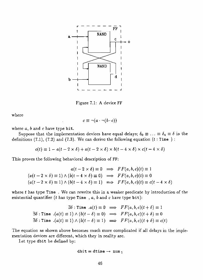
r ------.,FF I

NAND Ic

1--r-----1r-- 0

b ----11----1

L _

d

_ .J

Figure 7.1: A device FF

where

where a, band c have type bit.Suppose that the implementation devices have equal delays; 80 =... =84 == 8 in the

definitions (7.1), (7.2) and (7.3). We can derive the following equation (t : Time) :

c(t) = 1 - a(t - 2 x 8) + a(t - 2 x 8) x b(t - 4 x 8) x c(t - 4 x 8)

This proves the following behavioral description of FF:

a(t-2x8)-0 ==> FF(a,b,c)(t)=l

(a(t -2 x 8) = 1) /\ (b(t -4 x 8) = 0) ==> FF(a,b,c)(t) =0(a(t -2 x 8) =1) /\ (b(t -4 x 8) -1) ==> FF(a,b,c)(t) c(t -4 x 8)

where t has type Time . We can rewrite this in a weaker predicate by introduction of theexistential quantifier (t has type Time, a, band c have type bit):

:18: Time .a(t) == 0 ==> F F(a, b, c)(t + 8) _ 1

:18: Time .(a(t) =1) /\ (b(t - 8) == 0) ==> FF(a,b,c)(t + 8) _ 0

:18: Time .(a(t) =1) /\ (b(t - 8) == 1) ==> F F(a, b, c)(t + 8) _ c(t)

The equation as shown above becomes much more complicated if all delays in the implementation devices are different, which they in reality are.

Let type dbi t be defined by:

dbi t = dtime --+ num 1

46

•

•

•

Figure 7.2: Temporal abstraction from 0"1 to 0"2

where dtime is a time type such that D(dtime) = IN. Suppose that the delays are smallenough such that, for t : dtime, (t + 1) - t ~ 8, where 8 is the largest delay in theimplementation devices.

If we convert the specification in a, band c defined on bit to a specification in a', b'and c' defined on type dbit, then we will loose the represen tation of the delays because thegrain in D(dtime) is 'coarser' than the grain in D(Time ). The conversion from one timedomain to another is called temporal abstraction. It will be discussed in the next section.

7.4 Temporal abstraction

Temporal abstraction involves relating formal specifications that describe hardware behavior using different notions of discrete time. This kind of abstraction is used when a designdescription gives more detail about how a device behaves over time than is desired for itsabstract specification. With the mechanism of temporal abstraction, information about adevice's behavioral expressed in moments of time that are not of interest can be hiddenfrom the abstract specification, allowing the specification to concentrate on how the devicebehaves at significant or 'interesting' points of time.

In the simplest case of temporal abstraction, each single unit of discrete time at theabstract level of description corresponds to several units of time at the more detailed levelof description. Here, the abstract specification of a device defines its behavior at fewerpoints of time than the design description - i.e. the grain of discrete time is 'coarser' atthe abstract level than at the detailed level.

To express this in logic, we must specify for each single unit or step of 'high level' timea corresponding interval or sequence of steps of 'low level' time. For example, let t' be avalue of a high level time type O"ll and t be a value of a low level time type 0"2. Supposethat the unit of time t' to t' + 1 corresponds to the interval of time from t to t +n at themore detailed level of description.

In this case, high level time t' corresponds to low level time t and high level time t f +1corresponds with low level time t + n. This correspondence can be specified by defining

47

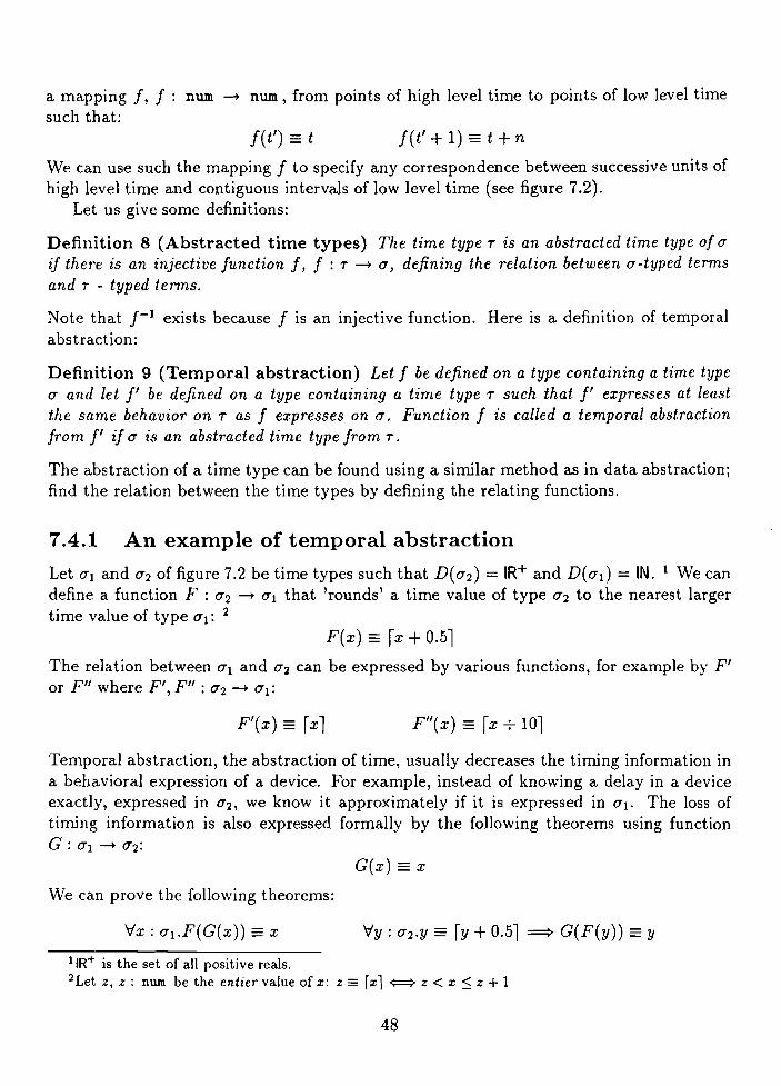
a mapping f, f : nwn -+ nwn, from points of high level time to points of low level timesuch that:

f(t') == t f(t'+l)==t+n

We can use such the mapping f to specify any correspondence between successive units ofhigh level time and contiguous intervals of low level time (see figure 7.2).

Let us give some definitions:

Definition 8 (Abstracted time types) The time type T is an abstracted time type of (7if there is an injective function f, f : T -+ (7, defining the relation between (7-typed termsand T - typed terms.

Note that f- 1 exists because f is an injective function. Here is a definition of temporalabstraction:

Definition 9 (Temporal abstraction) Let f be defined on a type containing a time type(7 and let f' be defined on a type containing a time type T such that f' expresses at leastthe same behavior on T as f expresses on (7. Function f is called a temporal abstractionfrom f' if (7 is an abstracted time type from T.

The abstraction of a time type can be found using a similar method as in data abstraction;find the relation between the time types by defining the relating functions.

7.4.1 An example of temporal abstraction

Let (71 and (72 of figure 7.2 be time types such that D((72) = IR+ and D((7d = IN. 1 We candefine a function F : (72 -+ (71 that 'rounds' a time value of type (72 to the nearest largertime value of type (71: 2

F(x) =rx + O.5l

The relation between (71 and (72 can be expressed by various functions, for example by F'or F" where F', F" : (72 -+ (71:

F'(x) == rxl F"(x) =rx -;-.lOl

Temporal abstraction, the abstraction of time, usually decreases the timing information ina behavioral expression of a device. For example, instead of knowing a delay in a deviceexactly, expressed in (72, we know it approximately if it is expressed in (71. The loss oftiming information is also expressed formally by the following theorems using functionG : (71 -+ (72:

G(x) =x

We can prove the following theorems:

'Vx: (71.F(G(x)) = x 'Vy: (72.y =ry + O.5l ::=::} G(F(y)) = y

llR+ is the set of all positive reals.2Let z, z: num be the entier value of x: z == [xl {:::=> z < x ~ z + 1

48

which is equivalent to:

This means that 0"1 and 0"2 are not isomorphic, so we can not prove the existence of antransformation of f defined on 0"2 if f is defined on 0"1 by using theorem 1. We have toprove the existence of the transformation of f by constructing it.

7.4.2 Temporal abstraction of the Flip-Flop

We can abstract the Flip-Flop from bit to num 1 with the conversion functions e.p: num 1 --+

bit and 'lj; : bit --+ num 1 defined by:

e.p(a) >..t:Time.a

::Jt : Time .'lj;(x) =x(t)

We can prove:e.p 0 'lj; :::::: I D num 1

The functions between bit and num 1 are not isomorphic; the temporal abstraction frombit to num 1 will result in an decrement in timing information. However, the specificationof device FF expressed by F F' : ( num 1)3 --+ num 1 is shorter:

a::::::O ====} FF'(a,b,c)_I

(a _1) 1\ (b == 0) ====} FF'(a,b,c) =0

(a =1) /\ (b:::::: 1) ====} FF'(a,b,c) =c

7.5 Time representation in sequences

A signal defined on a discrete timing domain can be expressed by a function over timebut also by a sequence. A representation of a signal as a sequence can result in a shorterexpression of temporal behavior. Johnson [Joh86] uses sequences to express signals. We willshow that the relation between an expression of a signal as a sequence and an expression ofa signal as a function over time is isomorphic. First, we will define sequences by a I-placetype operator seq and the corresponding operations on seq.

7.5.1 The type operator seq

In the following example we will use the type operator seq to express lists of terms 3. If 0"

is a type, then (0" )seq is the type of all sequences of O"-typed terms. Type (0" )seq has twotype constructors:

Nil: (O")seq

3Type operator seq is defined as 'sequence' in [Pau87, p. 117].

49

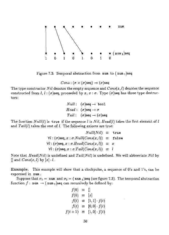
1 ° 1 ° 1

•

•°

•

•1

• num

Figure 7.3: Temporal abstraction from num to (num 1 )seq

Cons: (0" x (O")seq) -+ (O")seq

The type constructor Nii denotes the empty sequence and Cons(x, i) denotes the sequenceconstructed from i, i : (O")seq, proceeded by x, x : 0". Type (O")seq has three type destructors:

Null :Head:

Tail:

(0" )seq -+ booI

(0" )seq -+ 0"

(0" )seq -+ (0" )seq

The function Nul1(l) is true if the sequence 1 is Nil, Head(l) takes the first element of iand Tail(l) takes the rest of 1. The following axioms are true:

Null(Nii) true

Vi: (O")seq,x: O",Null(Cons(x, l)) - false

VI: (O")seq,x: O".Head(Cons(x,I)) = x

Vi: (O")seq, x : O".TaiI(Cons(x, 1)) _ 1

Note that Head(Nil) is undefined and Tail(NiI) is undefined. We will abbreviate Nil by[] and Cons(x, i) by [x] . 1.

Example. This example will show that a clockpulse, a sequence of O's and l's, can beexpressed in num.

Suppose that 0"1 = num and 0"2 = (num dseq (see figure 7.3). The temporal abstractionfunction f: num -+ ( num 1 )seq can recursively be defined by:

f(O) []f(O) - [x]f(t) - [1,1] . f(t)f(t) - [O,O]'f(t)

f(t + 1) - [1,0] . f(t)

50

where t: num and [x,y] abbreviates [x]. [y], for x,y: num1.The function I has an inverse:

1-1([]) =0

1-1 ([x]) =0

X == 1/\ Y = 0 => 1-1 ([x,y] ·1) = 1 + 1-1 (1)

X t= 1 Vy t= 0 => 1-1 ([x,y] ·1) =1-1([y] ·1)

The functions I and 1-1 formally define a discrete timing domain in num from a clockpulseexpressed in (num l)seq. Instead of a sequence I, 1 : (num l)seq, consisting of O's and l'swe get pulse number 1-1 (1) .

. 7.5.2 Sequences and functions over time

We will construct relation between infinite sequences and functions over time to prove thatboth representations of signals are isomorphic.

Let dtime be the time type such that D(dtime) = IN and let (O")sgnl be a type definedby:

(O")sgnl = dtime --+ 0"

where 0" is a type. We can define the conversion functions c.p (O")sgnl --+ (O")seq and'ljJ : (O")seq --+ (O")sgnl by

c.p(a) _ glue(a, O)1/J(l) - >.t: dtime.cut(l, t + 1)

where a : (O")sgnl and 1 : (O")seq, The functions glue: ((O")sgnl x num) --+ (O")seq andcut: ((a)seq x num) --+ (O")sgnl are defined by:

cut(l, l) cut(1, m + 1) _

glue(a,n)

Head(l)

cut(Tail(l), m)

[a(n)]· glue(a,n+ 1)

where n 2:: 0 and m 2:: 1. We can prove the following theorem:

Theorem 6 (O")seq ~ (O")sgnl

Proof of theorem 6 The prove of cut([xt, Xz, . .. ,Xk, . ..J, k) - Xk is easily obtained bymathematical induction to k. For 1, 1: (O")sgnl such that 1 == [xo, Xl,"'] we can derive:

c.p('ljJ(1))

{ def. 1/J }

c.p(>.t : dtime.cut(l, t))

51

{ prop. of cut}

<p(>.t : dtime.xt)

{ def. <p }

glue((>.t : dtime.xt),O)

{ def. glue}[xo] . glue((>..t : dtime.xt), 1)

{ calculus, def. glue}

[XO,Xl""]

I

For a, a : (0' )seq we can derive:

tP(<p(a))

{ def. <p }tP(glue(a, 0)){ def. glue}

tP([a(O)]· glue(a, 1)){ calculus, def. glue}

tP([a(O), a(I), ...J)

{ def·tP }

>.t : dtime.cut([a(O),a(I), .. .], t)

{ prop. of cut}

>.t : dtime.a(t)

a

This allows us to conclude:

tP 0 <p = I D(u)sgnl

(end of proof)What use does theorem 6 have? It shows that it doesn't matter which representation

for signals is used; by using <p and tP we can change an expression of signals in sequencesto an expression in functions over time and vice versa.

7.6 Behavioral abstraction

We have discussed structural abstraction (decomposition), data abstraction (transformation) and temporal abstraction. Only behavioral abstraction remains to be discussed.

52

The mechanism of behavioral abstraction serves to relate partial specifications to implementation descriptions that fully define the device's behavior, by showing that theyagree on the device's behavior for all states and inputs defined by the specification. Theneed for a mechanism of behavioral abstraction implies the need for a possibility to definespecification functions partially.

\Ve can express functions partially by introducing an element .Lq , for each type a,denoting undefinedness. 4 If x _ .Lq , x : a, then x is said to be undefined.

The introduction of a new element in every type implies that all operations have tobe redefined. We will not do this here, mainly because not every type has need for thesymbol .L. More about partial orderings, partial functions and the .L-symbol can be readin [Pau87].

A behavioral specification of a device can also be expressed partially by a predicate. Wealready used this form of behavioral abstraction. Let f : a -+ T be a function. Supposethat we only know a device A has a behavior that can be specified by f if the behavior onthe input lines satisfies a certain condition, say P( i), where i : a. So if the behavior onthe input lines is such that P( i) is true, then is device A specified by f( i). We can specifydevice A by:

::Ii : a.P(i) ===> A(i) = f(i)

where P is a predicate defined on a and f is a function. Device A is specified by functionG, G : a -+ T where

G = Ai: a.(P'(i) -+ f(i)I.L-r)

such that pI is a boolean function defined on a by P'( i) = true {::::::} P(i). Moreabout the use of predicates as behavioral specifications is found in [Gor86, Gor88].

4 See also page 26

53

Chapter 8

Concluding remarks

The previous chapters have shown methods to formalize the four kinds of abstractions asmentioned in the introduction of this thesis. We have shown how the behavior of a deviceis specified.

The actual derivation of specifications can be improved. The example of the addershowed that a good implementation is not always the implementation that directly canbe derived using the data-abstraction isomorphisms. How can a good implementation bederived? The following section suggests how designing by derivation is done using theabove-mentioned methods.

8.1 Specification and derivation

The specification of a device starts with an informal description of the device to be designed.This description can also contain descriptions of devices connected to the device to bedesigned. For example, a description of a memory device is needed in the design of amIcroprocessor.

8.1.1 The input type and output type

The next step is to determine the input values and output values that the device to bedesigned can have. We will define abstract types to cover the possible input values andoutput values of the device, where the input has a single type and the output also has asingle type, usually constructed with the sum type operator.

\Vhya single type and therefore a single input or output? Because the use of more thanone input or output is in fact a decision in the design process. Such decisions should bepostponed as long as possible. The introduction of new inputs and outputs by splitting theold ones is in fact forced upon us by the implementation, because each input or output linein the implementation, consisting of digital circuits, can usually contain only two values;Hand L.

54

-z_'I__DE_VIF(i,5)'

s =G(i,s)

Figure 8.1: An abstract device DEV

Example. In the design of a microprocessor, one can determine a type OPCODEto express the opcodes, a type ADDRESS to express the addresses, a type DATAto express data, I NTR to express the interrupts, et cetera. The abstract input typeof the microprocessor to be designed is the sum type of the types mentioned above:OPCODE +ADDRESS + INTR+ DATA+···. The abstract output type has a similarform.

8.1.2 Abstract operations and specifications

After we have defined the abstract input type and abstract output type, we can constructabstract functions on these types. The behavioral specification of the device to be designedcan be expressed in these functions defined on the abstract types. If necessary, we canintroduce a state variable together with its type. The device to be designed can now bespecified by a function F( i, s), where i describes the behavior of the input of the processorand s is the state variable (see figure 8.1). The 'next state' of s is defined by a functionG(i,s).

Example. In the design of the microprocessor mentioned previously, we have to definea state variable s to express the contents of the memory, the program counter, the accumulator, et cetera. The type of s is constructed such that it can handle data from theaccumulator, addresses of the program counter, and so on. It can be constructed likeDATA + ADDRESS + .". Let i be the variable specifying the input behavior of themicroprocessor. We can specify the processor by a function SCOMP(i, s) specifying thebehavior of its output and a function N XTSTATE( i, s) specifying the 'next state' of s.

8.1.3 Derivation

After the specification is constructed, we can try to derive an implementation. 1 First,we have to find elementary operations on the individual abstract types by decompositionof the specification. An example of an elementary operation defined on num is addition.

1An implementation is not always possible..

55

Multiplication is not an elementary operation, because it can be expressed by other operations on num. Decomposition can also lead to a smaller state variable and a less abstracttypes.

Example. In the design of the microprocessor we can construct elementary operationson DATA, like addition, on OPCODE, like an operator for selecting an microprocessorinstruction, and several other elementary operations.

Transformation. By trying to establish an isomorphism between abstract types andless abstract types, we prove the existence of a transformation of an abstract operation.This transformation is defined on the less abstract type and can also be decomposed toelementary operations on that type.

An isomorphism between types can not always be constructed, especially when theabstraction of the types is a temporal abstraction. In that case we have to construct afunction defined on the less abstract type to prove that a transformation of an abstractoperation exists.

By decomposition we can derive operations on the less abstract type, and so on - untilthe implementation types and operations are reached. This makes the abstract operationimplementable.

'Vhen all abstract operations used in the specification are proved to be implementablefunctions, then every function constructed from these is implementable abstract operationsan implementable function. This means that the behavioral specification of the device tobe designed is an implementable function. Its implementation is found by calculating thetransformation of the specification to the implementation type through the isomorphismsand operations between the specification type and implementation type.

Example. An isomorphism in the design of a microprocessor is the isomorphism betweenOPCODE, the type of the opcodes of the macro instructions, and opcode, the type of theopcodes of the micro instructions. If all the micro instructions are implementable, thenare the macro instructions also implementable, because a macro instruction is constructedfrom micro instructions.

Timing constraints. We have to be careful with temporal abstractions. A temporalabstraction usually decreases the timing information so it can hide timing difficulties thatmight occur in an implementation. We can bypass this problem if timing is introduced atan early phase of the derivation process. However, that does not eliminate the possibilityon the occurrence of timing difficulties.

8.2 Conclusions

This thesis has shown that the idea of abstraction is useful in the formal derivation ofdevices from their behavioral specification. We have seen that types are essential in the

56

derivation method. The proof of the existence of an implementation of an abstract behavioral specification simply by proving the isomorphism between the implementation typeand the abstract type in which the specification is expressed, is indeed a powerful mechanism. However, isomorphism between the implementation type and the abstract type cannot always be proved, especially when the abstraction is a temporal abstraction.

\Ve can try to avoid this by an early use of timing and the concept of signals, e.g. in thespecification. This has a major drawback; the complexity of the specification and derivationincreases. behavioral descriptions become unreadable and unmanageable. Timing remainsa problem that must be taken seriously. We could express signals by sequences, whichis in fact a good representation of signals without loosing to much temporal information.It is isomorphic to the representation of signals as functions defined on IN. However, thesearch for a better representation for signals isomorphic to the previously mentioned signalrepresentations continues.

However, isomorphic time types share the same properties as other isomorphic types.For any type (7, T, J.L we can prove (7 -+ T ~ (7 -+ J.L easily provided that T ~ J.L is true.We have discovered some isomorphisms, e.g. (num dm ~ num m, that can be extended tosignal types. Let time be a time type, then the following isomorphism is true:

time -+ (num l)m ~ time -+ num m

The isomorphism (7 -+ (T X J.L) ~ ((7 -+ T) X ((7 -+ J.L) allows us to conclude:

(time -+ num dm~ time -+ num m

This means that m implementation typed signals can be expressed by one num m - typedsignal. So, for the num 1 - typed signals Xl, ••• ,Xm there is one num m - typed signal a suchthat a(t) f--+ (XI(t), ... , xm(t)) for all t : time.

Many other isomorphisms can be found to define the relation between an implementation function and an abstract function. We could define some implementable operationson abstract types. If a specification of a device is expressed in implementable operationsdefined on abstract types, then we know that an implementation exists. We can evenderive it ! This derivation could be done automatically. So a behavioral specification ofa device expressed in implementable operations results in an implementation; a design ofthe specified device satisfying the specification.

8.3 Acknowledgements

First of all, I would like to thank Peter de Graaff for coaching and advising me and forthe necessary corrections in this thesis. I also would like to thank Cees Jan Koomen forsupervising and my parents for their support.

57

Bibliography

[Bou86] R. T. Boute. Current work on the semantics of digital systems. In G.J. Milneand P.A. Subrahmanyam, editors, Formal aspects of VLSI-design, pages 99-112,North-Holland, 1986.

[dG90] P. J. de Graaff. On the formal specification and verification of digital circuits.march 1990. Will be published in the proceedings of Euromicro '90 conference in1990, internal note Eindhoven Univ. Techn., fac. E.

[End72] H. B. Enderton. A mathematical introduction to Logic. Academic Press, 1972.

[Gor79] M. J. C. Gordon. The denotational description of programming languages, Anintroduction. Springer Verlag, 1979.

[Gor86] M. J. C. Gordon. Why higher order logic is a good formalism for specifyinghardware. In G.J. Milne and P.A. Subrahmanyam, editors, Formal aspects ofVLSI-design, pages 153-177, North-Holland, 1986.

[Gor88] M. J. C. Gordon. HOL; A proof generating system for Higher Order Logic. InG. Birtwistle and P. A. Subrahmanyam, editors, VLSI Specification, Verificationand Synthesis, pages 73-128, Kluwer Ac. Publishers, Boston, 1988.

[HD85] F. K. Hanna and N. Daeche. Specification and verification using Higher - OrderLogic. In C. J. Koomen and T. Moto-oka, editors, Computer Hardware DescriptionLanguages and their Applications, pages 418-433, IFIP, IFIP North Holland, 1985.

[HD86] F. K. Hanna and N. Daeche. Specification and verification using Higher - OrderLogic: A Case Study. In G.J. Milne and P.A. Subrahmanyam, editors, Formalaspects of VLSI-design, pages 179-213, North-Holland, 1986.

[Her89] J. M. J. Herbert. Formal reasening about the timing and function of basic memorydevices. In 1. J. M. Cleasen, editor, Applied formal methods for correct VLSIdesign, pages 668-687, IMEC-IFIP, IMEC-IFIP workshop organization, 1989.

[Joh86] S. D. Johnson. Digital design in a functional calculus. In G.J. Milne and P.A. Subrahmanyam, editors, Formal aspects of VLSI-design, pages 45-57, North-Holland,1986.

58

[MeI88] T. F. Melham. Abstraction mechanisms for hardware verification. In G. Birtwistleand P. A. Subrahmanyam, editors, VLSI Specification, Verification and Synthesis,pages 267-291, Kluwer Ac. Publishers, Boston, Univ. of Cambridge, 1988.

[Pau87] L.C. Paulson. Logic and Computation. Volume 2 of Cambridge tracts in theoreticalcomputer science, Cambridge University press, 1987.

[Sub88] P. A. Subrahmanyam. Towards a framework for dealing with system timing in VeryHigh Silicon Compilers. In G. Birtwistle and P. A. Subrahmanyam, editors, VLSISpecification, Verification and Synthesis, pages 159-215, Kluwer Ac. Publishers,Boston, AT & T Bell-labs, 1988.

59

Specification and derivation ofdigital circuits using...

Documents

Transcript of Specification and derivation ofdigital circuits using...