Spatiotemporal machine learning - University of...
22
Spatiotemporal machine learning Anand Rangarajan and Sanjay Ranka Dept. of CISE University of Florida
Transcript of Spatiotemporal machine learning - University of...

Spatiotemporal machine learning
Anand Rangarajan and Sanjay RankaDept. of CISE
University of Florida

Remote Sensing: Big Spatial Data
Spatial
Spectral
Temporal
AVIRIS (20m, 224B): On demand, airborne, 700km/hr.
1970’s 2000
Landsat-1 (MSS): 80m, 4B, 18 day revisit
AVHRR (1KM, 5B, 1 day)
ARIES (30m, 32B, 7 day)
MODIS (250m-1KM, 36B, 1-2 days)
1M (SPOT, IKONOS, WorldView)
Sub-meter (Aerial, …)
5TB/day – Heterogeneous data

Challenge
•How to map informal settlements (slums, barrios, shanty towns, …) in an efficient manner?
• Objects may be same (e.g., Buildings, Roads, …), but not the spatial patterns (neighborhoods)
Informal
Formal
Very High Resolution Imagery

Sample-based Spatiotemporal
Segmentation K-Means Clustering Graph partitioning
Classification Support vector machine ????
Unsupervised learning Pixel dictionary Superpixel dictionary
Permutation (acid test) Invariant Not invariant
Sample-based ML versus Spatiotemporal ML
Sample-based classification Spatial image classification
Expert labels

Novel Framework
• Superpixel formation• Superpixel descriptor• Building the Superpixel graph• Initializing the graph labels• Label refinement• Parallelization

Superpixel Descriptor
• Intensity histograms• Corner density • Size of Superpixels• Binary feature based on coarse scale tessellation
All these features are concatenated to obtain a 54 dimensional descriptor for each superpixel

Superpixel formation
• Parcellation into homogenous regions
• Huge reduction in data complexity

Semi-supervised Learning: Initializing the graph labels
• The expert labels a very few pixels (ground truth)• This sparsely available ground truth is used to
learn a classifier.• Several approaches are used:
– K- nearest neighbors (based on k-d trees)– SVM (we use a linear kernel in our framework)
• Once the classifier is obtained, rudimentary labels are obtained for all the superpixels

Label refinement
• Labels obtained in the previous step are rudimentary.• This can cause artifacts (neighboring regions
belonging to same class can get different labels).• Laplacian propagation is used to smooth the labels
obtained in the previous step.

Laplacian propagation
• Minimize the following cost function separately for each category:
– 𝑌𝑌𝑖𝑖 is 1 if the superpixel belongs to the category and 0 otherwise.
– 𝑋𝑋𝑖𝑖 is relaxed to take real values• Maximum value of 𝑋𝑋𝑖𝑖 for each category is used as the
final label for each superpixel.

Performance and Accuracy
• Our approach labels approximately 90% of the pixels correctly in 20 minutes for a 1000 x 1000 image patch while Citation KNN takes 27.8 hours and GMIL takes 3.1 hours for a 1000 x 1000 image patch, at a fixed grid size.
• Our approach does not require experimentation to obtain the right grid size which is an unsolved problem.
• Our segment boundaries correspond to natural object boundaries.

Parallelizaton
• Most of the steps are easily parallelizable using data decomposition techniques (Parallel versions using MPI, Apache Spark in development).
• Expect to be able to process 200 square km per core per day
• Using 1000 cores should result in processing of 200,000 sq km per day.
Manu Sethi, Yupeng Yan, Anand Rangarajan, Ranga Raju Vatsavai, Sanjay Ranka: An efficient computational framework for labeling large scale spatiotemporal remote sensing datasets. IC3 2014: 635-640Manu Sethi, Yupeng Yan, Anand Rangarajan, Ranga Raju Vatsavai, Sanjay Ranka: Scalable Machine Learning Approaches for Terrain Classication datasets. Submitted.

10.8K * 9.8K
2K * 2K patches
Combine results
35000 superpixels
Tessellation of Rio

Results

Corner density is negligible in forest regions but quite high in urban and slum regions. We use Harris corner detector for obtaining the corners.
Superpixel descriptor: Corner Density

Parallelization
• Most of the steps are easily parallelizable using data decomposition techniques (Parallel versions using MPI, Apache Spark in development).
• Expect to be able to process 200 square km per core per day
• Using 1000 cores should result in processing of 200,000 sq. km per day.
Manu Sethi, Yupeng Yan, Anand Rangarajan, Ranga Raju Vatsavai, Sanjay Ranka: An efficient computational framework for labeling large scale spatiotemporal remote sensing datasets. IC3 2014: 635-640Manu Sethi, Yupeng Yan, Anand Rangarajan, Ranga Raju Vatsavai, Sanjay Ranka: Scalable Machine Learning Approaches for Terrain Classication datasets. Submitted.

Images and Dictionaries: Coding, denoisingand registration
Source: SPIE
Image Patches3D, 4D and 5D blocksMixtures of HOSVDs
IEEE Trans. Image Proc. 2008, IEEE T-PAMI 2013Joint work with Arunava Banerjee
Research Q: Generalization to non-uniform tesselations?

Hyperspectral Imaging
The hyperspectral realm: Numerousbands at each pixelSegmentation, Unmixing andClassification: Spatiotemporal ML
Image Segmentation
EndmemberExtraction
Abundance Estimation Unmixing
GRENDEL (Graph-based EndmemberExtraction and Labeling
(Joint work with Paul Gader)
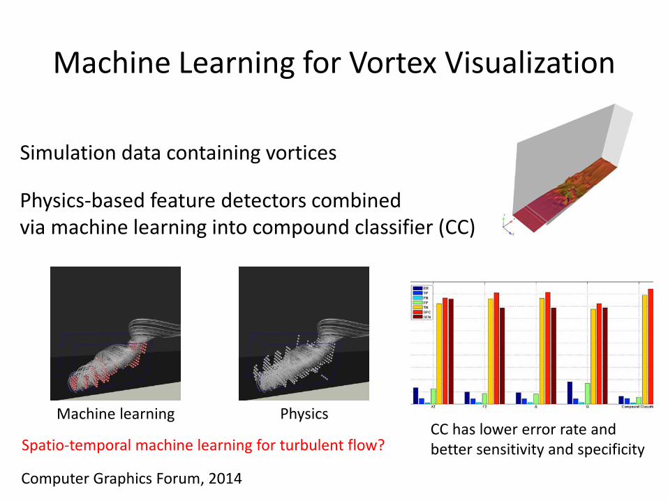
Machine Learning for Vortex Visualization
Simulation data containing vortices
Physics-based feature detectors combinedvia machine learning into compound classifier (CC)
Machine learning PhysicsCC has lower error rate and better sensitivity and specificity
Computer Graphics Forum, 2014
Spatio-temporal machine learning for turbulent flow?

Representation of Multilevel Structures

Making Waves With Shapes
• Quantize classical system Linear Schrödinger• Wave magnitude: Probability, Phase: Curve geom.• Apps: Correspondence, indexing, classification
Research Direction: Can other classical problemslike shortest paths on manifolds be “quantized”?
NSF 1143963: IEEE CVPR 2012, SIAM Math Anal. 2012
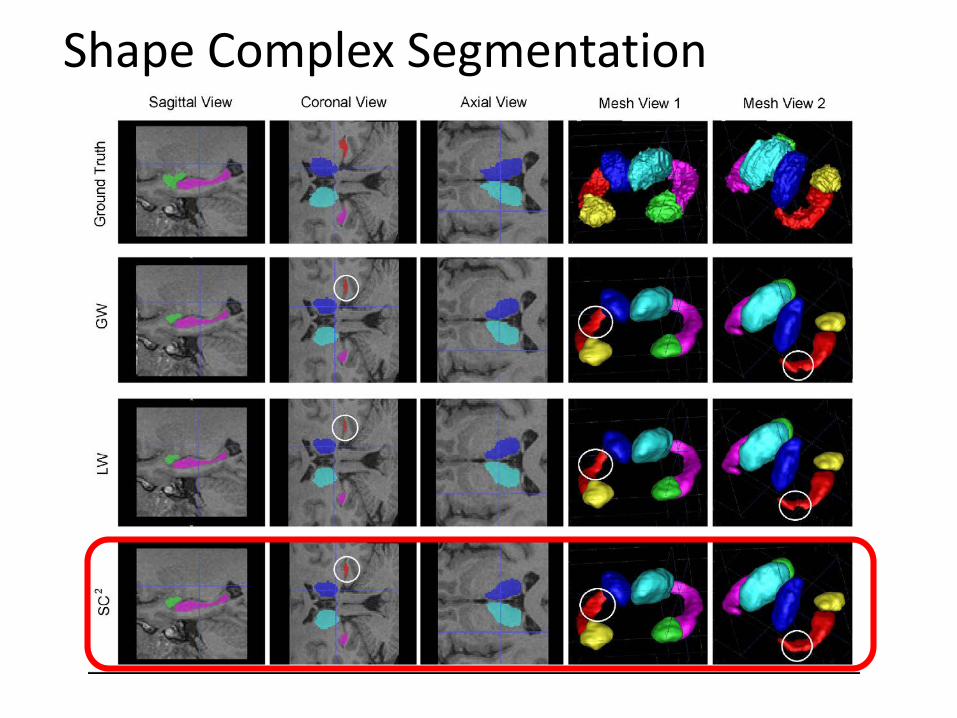
Shape Complex Segmentation