Electrical resistivity tomography for spatiotemporal variations of soil moisturein a precision irrigation experiment**

Yannis Mertzanides1,2* , Ioannis Tsakmakis2 , Evangelos Kargiotis1 , and Georgios Sylaios2

1Department of Chemistry, International Hellenic University, Aghios Loukas, 65404, Kavala, Greece 2Department of Environmental Engineering, Democritus University of Thrace, Vas. Sofias 12, 67100, Xanthi, Greecee

Received September 27, 2019; accepted June 14, 2020

Int. Agrophys., 2020, 34, 309-319doi: 10.31545/intagr/123943

*Corresponding author e-mail: mertzan@gmail.com**The research leading to these results has received funding from the European Community’s Seventh Framework Program (FP7/2007-2013) under grant agreement 311903 – FIGARO (Flexible and Precise Irrigation Platform to Improve Farm-Scale Water Productivity (http://www.figaro-irrigation.net/).

A b s t r a c t. Soil moisture temporal variations play a key role in the hydrological processes occurring in the unsaturated zone, which are critical for annual crop yields. The electrical resistivity tomography technique was applied in a field cultivated with cot-ton in northern Greece, thereby investigating its potential to serve as a reliable soil moisture-monitoring tool for precision irrigation in highly heterogeneous, clay-rich soils. Repeated surface resis-tivity measurements were made along two plant lines combined with soil water content measurements conducted with a reference gravimetric method and an electromagnetic sensor. Resistivity pseudo-sections were inverted to produce 2D resistivity mod-els, and time-lapse inversion algorithms were also used, to better calculate the temporal changes in subsurface soil resistivity. The results showed clear spatial and temporal changes in resistivity transects in accordance with rainfall/irrigation and dry periods. The soil resistivity data exhibited a power model relationship with gravimetric soil moisture point measurements and a fair correla-tion with electromagnetic sensor profiles.

K e y w o r d s: electrical resistivity tomography, non-intrusive soil measurements, soil moisture determination; heterogeneous clay-rich soils, water-saving technology

INTRODUCTION

Soil water has a fundamental role in the atmosphere-soil-plants interaction. Soil water has been a subject of intensive study over recent decades mainly due to its impact on plant growth and agricultural productivity (Rajkai et

al., 1997). During this time, significant developments in the instrumentation of classical soil water measurement through indirect methods have come about, based e.g., on the absorption of neutron radiation, heat conductivity and the electromagnetic (EM) properties of soils. However, these instruments provide point-scale data and have a limi- ted profiling capacity, while local phenomena such as soil discontinuities may add elements of uncertainty to the results of measurements (Oleszczuk et al., 2004; Dahan et al., 2007).

Geophysical methods seem to overcome these limita- tions, although this comes with the price ofa loss in accu- racy, as they extend the observable space in the mea-surements from the decimetre to the tens of meters scale (Reynolds, 2011). Due to the strong dependence of bulk electrical resistivity (ER) on soil water, ER measurements have been used for mapping the subsurface spatial inho-mogeneities caused by variationsin soil water content (Samouëlian et al., 2005). An analysis of resistivity data-sets with inversion techniques, have shown the capacity of electrical resistivity tomography (ERT) in producing 2D or 3D resistivity models, related to soil variability (Rossi et al., 2013) and spatial variation in soil moisture (Binley and Kemna, 2005). Repeated resistivity measurements with ERT over time, may also reveal the temporal variations in soil moisture (Zhou et al., 2001). Time-lapse ERT in con-junction with EM sensor surveys exhibit a strong potential in monitoring soil water changes (Michot et al., 2003; Calamita et al., 2012), root water uptake (Beff et al., 2013)

© 2020 Institute of Agrophysics, Polish Academy of Sciences

Y. MERTZANIDES et al.310

and root zone systems (Cassiani et al., 2015) in the unsat-urated zone. Moreover, automated systems with telemetric data transfer of 2D and 3D time-lapse ERT for monitoring moisture dynamics have been developed (Chambers et al., 2014). Rings et al. (2008) demonstrated the feasibility of using ERT monitoring calibrated with soil moisture sensors incorporating time domain reflectometry (TDR) technology, to quantify soil water content and applied depth-dependent regularization to reduce inversion artifacts. Schwartz et al. (2008) used a time-series of 2D electrical resistivity and 1D TDR data and through a modified form of Archie’s law, quantified field-scale soil moisture in heterogeneous clayey soils. However, as shown in the review study of Friedman (2005), who presented theoretical results and experimental evidence from saturated and unsaturated soils, the development of reliable physical models requires site-specific calibrations in the laboratory. Although ERT has been successfully applied for soil water content deter-mination in soils with a limited clay content (Michot et al., 2003; Beff et al., 2013; Dahlin et al., 2014), limited studies examine the resistivity-soil moisture relationship in soils with increased clay mineral content (> 40%, e.g., Satriani et al., 2012). As the presence of clay makes the soil mate-rial matrix become jointly responsible with soil moisture ionic strength for the electrolytic phenomena produced during soil electrical conductivity measurements, a num-ber of different formulations in the resistivity-water content models have been suggested. Modified forms of Archie’s law - either through the addition of a parameter (Waxman and Smits, 1968) or setting clay-dependent fitting parame-ters (Schwartz et al., 2008) - other second order polynomial expressions (Kalinski and Kelly, 1993), exponential (Zhu et al., 2007) or linear (Michot et al., 2003) relationships and pedotransfer functions by integrating the soil char-acteristics (Brillante et al., 2014) have been proposed to include soil matrix conductivity. Brillante et al. (2015), in reviewing the methodologies for modelling the resistivity- water content relationship, mentioned the validity issues that appear in the calibration process whether laboratory or in-field resistivity data are used. Calamita et al. (2012) summarized the main characteristics of the most relevant published studies, showing that power, exponential and second order polynomial functions are most commonly used to fit the electrical resistivity – soil moisture relation-ship. However, the differences between these three types of models are often statistically insignificant and a regression analysis with different linear and non-linear models could be useful. Moreover, precision agriculture studies usually focus on a narrow range of soil moisture content, from 20 to 35% between the permanent wilting point and the field capacity, where simple linear relationships are very often sufficient (Michot et al., 2003).

In this study, time-lapse surface ERT data were related to soil water content data, which was obtained from gravi- metric and EM sensor measurements. The objectives of

the study were (i) to provide a regional evaluation of sur-face ERT monitoring on spatiotemporal variations of soil moisture in a complex clayey field, (ii) to set up simple calibration relationships between ERT and soil moisture measurements and (iii) to assess the potentiality of the ERT technique for serving as a precision irrigation monitoring tool for intensive farming in Mediterranean complex soil systems.

MATERIAL AND METHODS

Soil electrical resistivity is mainly influenced by soil water content, but it also depends on a number of oth-er factors like pore water salinity, clay content, lithology, soil density, porosity, soil temperature and organic matter (Samouëlian et al., 2005). In order to describe the relation-ship between electrical resistivity and soil water content, petrophysical models linking the electrical and hydraulic properties of soils and rocks have been proposed (Hubbard and Rubin, 2005). For coarse to medium grained soils and rocks the fundamental relationship is Archie’s law (Archie, 1942):

ρ = αρw Φ-m S -n, (1)

where: ρ is the soil electrical resistivity (Ωm); S is the water saturation of the soil (the volume fraction of soil water content to soil porosity); ρw is the electrical resistivity of pore water (Ωm); Φ is the porosity of the medium; α is an adjustment parameter; m is the cementation factor; n is the saturation exponent. Generally, 0.5 ≤ α ≤ 2.5, 1.3 ≤ m ≤ 2.5, and n ≈ 2.0 (Reynolds, 2011). This semi-empirical relation-ship has been successfully used for applications in porous media poor in clay (Nijland et al., 2010). The saturation degree, S, may be expressed as S = θ/Φ, where, θ is the soil water content (cm3 cm-3), thus, Eq. (1) becomes:

ρ = αρw Φn-m θ -n. (2)Assuming that the soil properties and pore-water resi-

stivity are homogeneous, Eq. (2) could be expressed as a simplified Archie’s law (Yamakawa et al., 2012):

ρ = Aθ -n, (3)where: A = αρw Φn-m, is a constant.

In order to better understand the interrelationship between soil electrical resistivity (ρ) and its water content (θ) in clayey soil horizons an experiment was designed to perform successive ERT measurements, aiming to provide insights concerning the capacity of ERT to act as an opera-tional precision irrigation tool contributing to water saving at a farm level. Indeed, although previous studies have shown the potential of ERT to adequately monitor the root system of trees (Fan et al., 2015; Ain-Lhout et al., 2016), studies designed to determine ERT potential to monitor the annual crop root growth in clay-rich soils are scarce.

ERT FOR SPATIOTEMPORAL VARIATIONS OF SOIL MOISTURE IN A PRECISION IRRIGATION EXPERIMENT 311

As soil temperature influences the interpretation of soil electrical resistivity profiles in terms of soil water con-tent, five soil temperature sensors (Decagon 5TM) were installed at 30 cm depth in the experimental field plot. Soil temperature impact followed the Keller and Frischknecht (1966) analysis:

ρΤ = ρ25/(1+α (Τ-25)), (4)

where, ρΤ is the electrical resistivity at temperature T, ρ25 is the electrical resistivity at T = 25oC and, α is an empiri-cal coefficient that, as reported in the literature (Keller and Frischknecht, 1966; Samouëlian et al., 2005; Brunet et al., 2010), could be considered to be equal to 0.025oC-1.

The experiment conducted during 2014 in a cotton field located at Xanthi rural area (41.046oN, 24.892oE) in the Thrace region, Northern Greece, covered an area of 1 ha. A field texture analysis revealed the stratification of the soil into two major horizons: an upper horizon rang-ing from the surface to a 35-55 cm depth characterized as a sandy clay layer; a bottom horizon starting from a 35-55 cm depth and continuing down to 1m dominated by heavy soils (clay, clay loams).

During the cultivation period, May to October, the experimental field received a total water amount of 492; 345 mm of precipitation and 147 mm of irrigation water delivered by a traveling gun sprinkler system).

The ERT survey was carried out between June and October 2014, on two parallel investigation lines, A and B, oriented in a north/south direction, and positioned along two cotton plant rows. The particle size distribution for the disturbed soil samples collected near the centre of the two investigation lines in the field test site, as calculated by the Bouyoucos hydrometer method (Bouyoucos, 1962), is shown in Table 1. The geoelectrical imaging system that was used was a 4-channel ABEM Terrameter LS instru-ment with two multi-electrode cables (21 take-outs per cable). Each measurement line had 41 stainless steel elec-trodes spaced at 25 cm intervals and it was 10 m long. The electrodes were permanently installed in the field shortly after sowing throughout the whole survey in order to avoid mispositioning in subsequent measurements. A total num-ber of 27 repeated resistivity measurement campaigns were

conducted (initial ERT measurement 12th of June – final ERT measurement 11th of October), using the gradient and the dipole-dipole array configuration, covering the grow-ing season of 2014. An effort was made to achieve daily stepwise monitoring of time periods that included rainfall and/or irrigation events. Although both array types are suit-able for multichannel-recording configurations and when initially tested in the field they both produced similar resis-tivity models, for further analysis the gradient electrode configuration was used due to: a) advantages in resolution (each dataset contained 512 measurements as compared to 348 measurements in each dipole-dipole array dataset), b) greater depth of investigation (about 1.80 m deep compared to about 1.50 m for the dipole-dipole array), c) although the dipole-dipole array has relatively high anomaly effects it often produces a lower signal-to-noise ratio compared to the gradient array and d) the sensitivity pattern of the gradient array that is more suitable for sensing horizontal structures (like the soil structure of the experimental field) than that of the dipole-dipole array that is more suitable for vertical and dipping structures (Dahlin and Zhou, 2004).

After a primary process to exclude possible low-quali-ty resistivity data (very little in our ERT survey, appearing only during days where top soil was very dry and cracked), inverse modelling was applied in order 2D resistivity sections to be produced. The least-squares smoothness-con-strained (L2-norm) inversion method (Loke and Barker, 1996) for each resistivity dataset was applied. The tem-poral differences of subsurface resistivity due to soil moisture changes were imaged by applying joint inversion techniques. To minimize the artifacts created by numeri-cal inaccuracies when inversion takes place, time-lapse resistivity data files were produced (Loke, 2010) and the inversion model at the final iteration was based on a start-ing model utilizing the data collected on 12 June 2014 as a reference dataset. A least-squares smoothness-constraint in the differences of model resistivity values between the initial and the time-lapse model and an equal-weight time-constraint, minimizing the temporal changes in the model and the RMS data error, were used. For the inverse and time-lapse analysis, the RES2DINV software package was applied (Loke and Barker, 1996).

In parallel with the ERT measurements, soil samples for the determination of the volumetric soil water content (VWC) via the gravimetric reference method were collect-ed on 9 occasions from 30, 60 and 80 cm depths during the cultivation period. Soil samples were collected on the periphery of a circle with a centre that coincided with the central point of each investigation line and with a radius about 35 cm. Due to the limited number of soil samples that could be collected from the field near the ERT lines, a more extended soil water content measurement sur-vey was conducted, using a pre-calibrated capacitance sensor probe, named Diviner 2000 (Frequency Domain Reflectometry Sensor FDR), through two PVC access tubes

Ta b l e 1. Particle size distribution for soil samples collected near the center of the two investigation lines in the field test site, as calculated by Bouyoucos hydrometer method

Depth (cm)Sand Silt Clay

(%)Line A

0 – 55 49.2 13.1 37.755 – 100 42.8 15.6 41.6

Line B0 – 55 46.2 16.1 37.7

55 – 100 44.0 17.2 38.8

Y. MERTZANIDES et al.312

allowing measurements down to 1 m (Tubes A and B), per-manently installed in the soil, positioned 25 cm alongside the centre of the two investigation lines.

The ER inverted values and the measured gravimet-ric water content were subjected to a regression analysis in order to obtain site-specific empirical relationships able to predict soil water content via ER. Initially, the data obtained from each depth and line were regressed individ-ually. Successively, the data from the deeper layers (60 and 80 cm) at each line and then for both lines were analysed together. Lastly, the gravimetric bulk datasets (the samples from all depths) collected for each line separately (e.g. line A and line B) and then for both lines were combined and regressed.

Similarly, the resistivity values (extracted from the cen-tral dataset column of each ERT profile) at depths of 30, 60 and 80 cm, were correlated with the corresponding Diviner 2000 soil water content measurements. As Calamita et al. (2012) pointed out, the scientific literature showed that such non-linear models as second order polynomial expression, power and exponential function, are most commonly used to fit the soil moisture – resistivity relationship. The power law regression model, - θ = aρb, where a and b are empirical constants implicitly containing the soil and water charac-teristics (i.e. porosity, salinity, temperature) and assumed to be invariant with time – was fitted to a) line A and tube A dataset; b) line B and tube B dataset and c) both lines and both tubes datasets. The empirical constants a and b, do not retain the interpretability of each parameter of Eq. (2), but they allow us to use the power regressionmodel (Brillante et al., 2014).

The coefficient of determination (R2) was used as a mea- sure of the goodness-of-fit between the gravimetric/Diviner 2000 soil water content and ER.

RESULTS AND DISCUSSION

The inverted resistivity images produced by the gradi-ent and dipole-dipole configuration for lines A and B on June 12, 2014 are presented in Fig. 1. In both lines, the resistivity values are notably low, ranging between 4 and 24 Ωm, indicating an increased water and clay content within the soil profile, although differences in the geoelec-trical structure may also be observed. This resistivity range falls within the previously reported values for clayey soils with a soil volumetric water content of between 15 and 30% (McCarter, 1984; Fukue et al., 1999). Both configu-rations, exhibit in line A, three distinct resistivity zones: An uppermost very thin layer, up to 30 cm in thickness, consisting of resistivity values of between 10 and 15 Ωm; an intermediate layer, from 30-100 cm deep, consisting of very low resistivity values of between 4 and 10 Ωm and a bottom zone with higher values of resistivity ranging from 10 to 24 Ωm. Soil stratification at the upper soil layers, is consistent with the soil textural analysis results, indicating that the lower ER values measured at depths below 30 cm are due to differences in the soil water content, soil tem-perature and an increase in the soil clay content (Calamita et al., 2012). Similar resistivity profiles appear for both configurations in line B, where the two uppermost resistivi-ty zones are significantly more distinct than the bottom one.

Fig. 1. Initial ERT 2D models for lines A and B measured on 12 June 2014, using the configurations: a) the gradient and b) the dipole-dipole.

Resistivity (Ωm)

ERT FOR SPATIOTEMPORAL VARIATIONS OF SOIL MOISTURE IN A PRECISION IRRIGATION EXPERIMENT 313

The average soil temperature at 30 cm depth during the ERT monitoring survey was calculated to be 25.9 ± 2.3oC and the soil temperature impact according to Eq. (4) resulted in a deviation of 5.3 ± 2.6% in ER values. Since electrical resistivity is also related to the mobility of the ions present in soil water, the interpretation of ERT images requires a knowledge of the concentration of dissolved ions. Moreover, the different ions present in the soil solu-tion do not affect the conductivity in the same way because of differences in ion mobility (Samouëlian et al., 2005). According to Van Dam and Meulenkamp (1967) who con-sidered the soil resistivity values of 40, 12 and 3 Ωm as being representative of fresh, brackish and saline water, the very low resistivity values (4 to 10 Ωm) that appear in the intermediate layer from 30-100 cm deep, may also indicate salinization of the groundwater (the experimental field was located 13 km north of the coastline and 13 km west of a lagoon) although farmland salinity may also be involved. The occurrence of seawater intrusion is supported by the high electrical conductivity values (> 3 000 μS cm-1) and high concentrations of chlorides (1.144 mg l-1) and sul-phates (240.81 mg l-1) that were measured in samples of the drilling-irrigation water of the experimental site.

The RMS errors in all inversion models were found to be low, ranging from 2 to 3% and only when the resisti- vity measurements were conducted in very dry topsoil, the inversion RMS errors increased by up to 6%. The geoelec-trical structure observed in the initial ERT models seems to reoccur in the subsequent 26 resistivity images on both lines, with fluctuations in resistivity values being observed on dry and wet days during the season. To gain a semi-quan-titative insight into the reliability of the inversion results, the subsurface sensitivity plot of the inversion model was calculated (Fig. 2). The sensitivity value is a measure of the amount of information about the resistivity of a mod-el block contained within the measured dataset. We know from theory, that the higher the sensitivity value, the more

reliable is the model resistivity value and, in general, the cells near the surface usually have higher sensitivity values because the sensitivity function has very large values near the electrodes (Loke, 2010). The sensitivity plot of Fig. 2 seems to follow these general rules. Moreover, the vertical decrement of sensitivity indicates the very low resistivity conditions of the soil.

Nine (out of a total number of twenty seven) ERT sections collected at various occasions during the cotton growing season are shown in Fig. 3: a) Initial resistivity measurement (12 June), b) at the beginning of a dry period (25 July), c) just before the first irrigation event (8 August), d) a few days after the first irrigation event (13 August), e) just before the second irrigation event (25 August) f) a few days after the second irrigation event (29 August), g) just after the third irrigation event (1 September), h) a few days after the third irrigation and heavy rainfall events (10 September) and i) the final resistivity measure- ment a few days after the final irrigation event (11 October). These selected examples represent extreme cases of resis-tivity fluctuation over the monitoring period, corresponding to the turning points of soil moisture temporal variation. The initial resistivity patterns (measured on 12 June 2014) on both lines were maintained throughout the monitoring period, but a gradual change in the magnitude and size of the resistivity zones are also distinct. The temporal varia-tions of resistivity sections were also studied by applying time-lapse inversion analysis for all the measured data-sets. The percentage variations (in the range of -100% to +100%) of the resistivity models for the aforementioned days of measurements (25 July, 8 August, 13 August, 25 August, 29 August, 1 September, 10 September and 11 October), relative to the initial ERT measurement on 12 June 2014, are shown in Fig. 4, and seem to follow cor-responding irrigation/rainfall and drying events during the monitoring period. This is also supported by the layered form of the high (when the soil is becoming dry as shown

Fig. 2. Plot of the subsurface relative sensitivity and datum point positions of the ERT model generated from the gradient array geome-try and inversion parameters used in this study for blocks of equal size. Sensitivity values (average value: 1.90) came from the Jacobian matrix of the last inversion of the initial ERT dataset of 12 June 2014.

Y. MERTZANIDES et al.314

Fig. 3. ERT 2D models from lines A and B measured during the 2014 cotton cultivation period with gradient configuration on: a) 12 June, b) 25 July, c) 8 August, d)13 August, e) 25 August, f) 29 August, g) 1 September, h) 10 September and i) 11 October.

Resistivity (Ωm)

ERT FOR SPATIOTEMPORAL VARIATIONS OF SOIL MOISTURE IN A PRECISION IRRIGATION EXPERIMENT 315

Fig. 4. Time-lapse inversion resistivity 2D models, for lines A and B, showing the percent change in resistivity relative to the ini-tial ERT measurement on 12 June 2014: a) 25 July, b) 8 August, c) 13 August, d) 25 August, e) 29 August, f) 1 September, g) 10 September and h) 11 October.

Change in resistivity (%)

Y. MERTZANIDES et al.316

in Fig. 3b, c, e and i) and the low (when the soil is becoming wet as shown in Fig. 3g and h) resistivity zones that seem to move vertically downwards from the ground surface to the unsaturated zone 5. The vertical extent of these high resistivity zones, besides soil evaporation, might also be partly attributed to the water and dissolved ions uptaken by the plant root system, a process observed up to a depth of 1 m. This is consistent with the findings of Tsakmakis et al. (2019) who showed that the maximum cotton rooting depth in these soils extends up to 1.15 m. The gentler temporal

differences in the resistivity profiles of line B compared to line A (shown in Figs 1 and 2), might reflect soil inhomoge-neities, due to differences in soil compaction (e.g. from the passage of agricultural machines or other agricultural prac-tices), an argument that is supported by the observations of compacted zones during drilling for soil samples.

The average, maximum and minimum volumetric water content and soil ER values during the combined ERT mea-surements – soil sampling surveys, are presented in Table 2. The average VWC was found to be significantly higher at depths of 60 and 80 cm as opposed to 30 cm in both lines (approximately 40% in line A and 33% in line B). The vol-umetric water content at depths of 60 and 80 cm, fluctuated roughly between 21 and 44% in line A and approximately 25 and 34% in line B. There were similar trends in ER val-ues, where in line A (for depths of 60 and 80 cm) ER was ranged approximately between 4 and 19 Ωm, whilst in line B they were between 3 and 8 Ωm. In general, high values of VWC correspond to low ER values, following the basic theory principle that increased soil moisture corresponds to lower ER values (Brillante et al., 2015). On the other hand, observations have shown that the maximum values of VWC (equal to 43.77 and 35.07%, which were measured at a depth of 80 cm in lines A and B respectively), do not cor-respond to the minimum ER values (~7.41 and 4.73 Ωm, respectively). Additionally, on the dryer days (when the minimum VWC values were found at the levels of 23.42 and 25.10%, respectively for lines A and B), the respective ER values were not at their maximum but equal to 18.89 and 6.20 Ωm, respectively. The results above indicate that there are other additional factors affecting the ER measure-ments, other than soil moisture (Samouëlian et al., 2005).

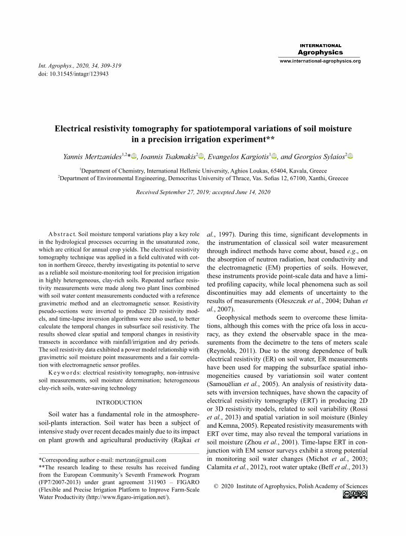
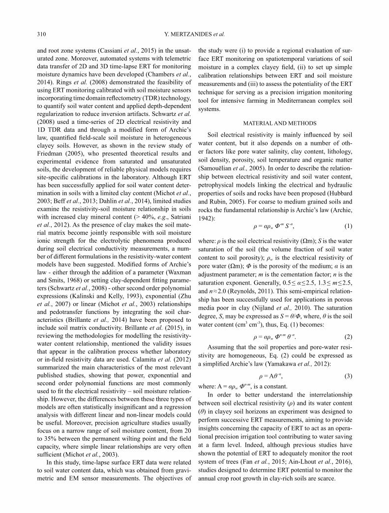
The regression analysis results, between ER and VWC, are presented in Table 3 and illustrated in Fig. 5. When the data for each depth and line were analysed separately, the coefficient of determination exhibited extreme spatial vari-ations (from R2 = 0.78 to R2 = 0.07 which shows no power model fitting), in both the horizontal (between the two measuring lines) and vertical (different depths) plains. The results of a regression analysis between ER and Diviner 2000 soil water content measurements are shown in Fig. 6, where no substantial differences are observed, nei-ther in regression parameters ( for line A and for line B) or in the coefficients of determination (R2 = 0.72, n = 84 for line A, R2 = 0.69, n = 120 for line B) between the data-sets of the two lines. Calamita et al. (2012), used a power low model to regress soil electrical resistivity against soil water content from TDR measurements for a group of dif-ferent locations in Italy containing silty clay and clay soils and reported R2 values between 0.56 and 0.70 and a and b values ranging from 50.15 to 70.64 and -0.31 to -0.15, respectively. These values are of the same magnitude as those estimated within the framework of the current study.

Ta b l e 3. Results of power model fitting (VWC = aERb) between ER and VWC for the various dataset combinations

Line Depth(cm) n a b R2

A 30 9 21.90 ± 6.06 -0.08 ± 0.11 0.07A 60 9 54.04 ± 11.97 -0.28 ± 0.11 0.50A 80 9 135.80 ± 41.47 -0.65 ± 0.13 0.78B 30 9 79.25 ± 49.87 -0.49 ± 0.25 0.38B 60 9 41.60 ± 4.72 -0.21 ± 0.07 0.53B 80 9 36.70 ± 5.62 -0.09 ± 0.10 0.11A 60-80 18 61.83 ± 11.39 -0.33 ± 0.09 0.48B 60-80 18 39.64 ± 3.76 -0.16 ± 0.06 0.30A All 27 57.77 ± 13.60 -0.35 ± 0.11 0.31B All 27 46.72 ± 3.56 -0.27 ± 0.04 0.65

A-B All 54 48.41 ± 4.61 -0.28 ± 0.05 0.42

Ta b l e 2. Average, maximum and minimum volumetric water content and electrical resistivity values, measured at depths of 30, 60 and 80 cm at lines A and B during the parallel ERT-soil sam-pling campaigns (n = 9)

Line Depth(cm) Ave SD Max Min

VWC (%)

A30 18.00 3.06 21.94 13.7760 29.84 6.28 41.87 23.4280 30.09 7.29 43.77 21.08

B30 22.78 5.32 32.86 17.7760 30.34 2.95 34.44 25.1080 31.90 2.43 35.07 27.99

Electrical resistivity (Ωm)

A30 14.15 8.25 29.11 6.4960 9.49 5.04 18.89 4.2980 11.29 3.96 18.12 7.33

B30 13.80 4.79 22.78 9.9260 4.92 1.70 8.26 2.7980 4.82 1.34 7.48 3.01

Ave – average, SD – standard deviation, Max – maximum, Min – minimum.

ERT FOR SPATIOTEMPORAL VARIATIONS OF SOIL MOISTURE IN A PRECISION IRRIGATION EXPERIMENT 317

The regression parameters in both lines A and B, are quite similar for a depth of 60 cm; the values of parame-ters a and b in line A, equal 54.04 and -0.28 respectively and in line B,41.60 and 0.21, while R2 is 0.50 for line A and 0.53 for the line B sub-dataset. It is noteworthy, that in line A, the best fitting was obtained at a depth of 80 cm (R2 = 0.78) and the worst (a regression analysis showed no power model fitting - R2 = 0.07) at the depth of 30 cm, whilst in the case of line B the opposite pattern was ob served (Table 3). Evett et al. (2012), regressed gravimetric soil water content data with FDR sensor raw measure-ments (frequency), obtained from a 2 m deep soil profile and found that the derived equations varied significantly in terms of slope and intercept with depth. They attributed this

finding to the sensitivity of the FDR sensors to the inherent bulk soil electrical resistivity and the decrease of the latter with depth, meaning that the increase in the FDR sensor’s raw measurements did not reflect an actual increase in the water content of the surrounding soil but to a decrease in the inherent soil electrical resistivity. Consequently, with the discrepancies observed in the current study, when soil resistivity was correlated to the gravimetric soil water con-tent at different depths, this could be related to the spatial variations of the inherent bulk soil resistivity in the verti-cal (variations at a, b and R2 components with depth) and horizontal (variations at a, b and R2 components at the same depth-different lines) dimension within the field. This conclusion is further strengthened by the fair correlation between the resistivity and Diviner 2000 measurements determined for each line as well as their bulked dataset (R2 > 0.67) (Table 2).

CONCLUSIONS

The results of the current work indicated that:1. The surface 2D electrical resistivity tomography

monitoring survey recorded rich static and dynamic infor-mation from the soil-water-plants system and its response to wetting and drying events. Inverse analysis revealed clear spatial and temporal changes in soil resistivity that reflected the textural/structural inhomogeneities of the soil profiles, the extent of cotton plant roots and the water flow in the unsaturated zone.

2. Both spatial and temporal changes in soil resistivity were efficiently and quite easily identified but the attempt to quantitatively interpret them came up against a number of uncertainties that need to be discussed.

3. The calibration relationships that were revealed after fitting electrical resistivity and moisture data derived from gravimetrical analysis and capacitance sensor probe surveys, despite their site-specific character and accuracy issues in some sub-datasets, contributed to our understand-ing of water infiltration and redistribution.

4. Further investigation, in incorporating additional information (soil temperature, borehole and cross-borehole electrical resistivity tomography arrays measurements, pore water conductivity etc.) collected in the field with inverse analysis constraints of resistivity datasets, may improve the efficiency of electrical resistivity tomography as a soil moisture monitoring technique.

ACKNOWLEDGEMENTS

The authors wish to thank Pioneer Hi-Bred Hellas for providing the cotton seeds for this experiment.

Conflict of interest: The authors do not declare conflict of interest.

Fig. 5. Power model fitting curves between gravimetric water content and ER for the depths of 30, 60 and 80 cm at: a) line A and b) line B.

Fig. 6. Power model fitting curves between VWC (measured with Diviner 2000) and ER for lines A and B.

Y. MERTZANIDES et al.318

REFERENCES

Ain-Lhout F., Boutaleb S., Diaz-Barradas M.C., Jauregui J., and Zunzunegui M., 2016. Monitoring the evolution of soil moisture in root zone system of Argania spinosa using resistivity imaging. Agric. Water Manag., 164, 158-166. https://doi.org/10.1016/j.agwat.2015.08.007

Archie G.E., 1942. The electrical resistivity log as an aid in deter-mining some reservoir characteristics. Trans. Am. Inst. Mining, Metallurgical Petroleum Eng., 146, 54-62. https://doi.org/10.2118/942054-g

Beff L., Günther T., Vandoorne B., Couvreur V., and Javaux M., 2013. Three dimensional monitoring of soil water con-tent in a maize field using electrical resistivity tomography. Hydrol. Earth Syst. Sci., 17, 595-609. https://doi.org/10.5194/hess-17-595-2013

Binley A.M. and Kemna A., 2005. DC resistivity and induced polarization methods. In: Hydrogeophysics, Water Sci. Technol. Library (Eds Rubin Y., Hubbard S.S.), Ser 50, Springer, New York. https://doi.org/10.1007/1-4020 -3102-5_5

Bouyoucos G.J., 1962. Hydrometer method improved for making particle size analyses of soils. Agron. J., 54, 464-465. https://doi.org/10.2134/agronj1962.00021962005400050028x

Brillante L., Bois B., Mathieu O., Bichet V., Michot D., and Lévêque J., 2014. Monitoring soil volume wetness in het-erogeneous soils by electrical resistivity - A field-based pedotransfer function. J. Hydrol., 516, 56-66. https://doi.org/10.1016/j.jhydrol.2014.01.052

Brillante L., Mathieu O., Bois B., van Leeuwen C., and Lévêque J., 2015. The use of soil electrical resistivity to monitor plant and soil water relationships in vineyards. Soil 1, 273-286. https://doi.org/10.5194/soil-1-273-2015

Brunet P., Clement R., and Bouvier C., 2010. Monitoring soil water content and deficit using electrical resistivity tomog-raphy (ERT) – A case study in the Cevennes area, France. J. Hydrol., 380, 146-153. https://doi.org/10.1016/j.jhydrol. 2009.10.032

Calamita G., Brocca L., Perrone A., Piscitelli S., Lapenna V., Melone F., and Moramarco T., 2012. Electrical resistivity and TDR methods for soil moisture estimation in central Italy test-sites. J. Hydrol., 454-455, 101-112. https://doi.org/10.1016/j.jhydrol.2012.06.001

Cassiani G., Boaga J., Vanella D., Perri M.T., and Consoli S., 2015. Monitoring and modelling of soil-plant interactions: the joint use of ERT, sap flow and eddy covariance data to characterize the volume of an orange tree root zone. Hydrol.Earth Syst. Sci., 19, 2213-2225. https://doi.org/10.5194/hess-19-2213-2015

Chambers J.E., Gunn D.A., Wilkinson P.B., Meldrum P.I., Haslam E., Holyoake S., Kirkhacm M., Kuras O., Merritt A., and Wragg J., 2014. 4D eletrical resistivity tomography monitoring of soil moisture dynamics in an operational railway embankment. Near Surf. Geophys., 12, 61-72. https://doi.org/10.3997/1873-0604.2013002

Dahan O., Shani Y., Enzel Y., Yechieli Y., and Yakirevich A., 2007. Direct measurements of floodwater infiltration into shallow alluvial aquifers. J. Hydrol., 344, 157-170. https://doi.org/10.1016/j.jhydrol.2007.06.033

Dahlin T., Aronsson P., and Thörnelof M., 2014. Soil resistivity monitoring of an irrigation experiment. Near Surf. Geophys., 12, 35-43.

Dahlin T. and Zhou B., 2004. A numerical comparison of 2D resistivity imaging with 10 electrode arrays. Geophys. Prospect., 52, 379-398. https://doi.org/10.1111/j.1365-2478. 2004.00423.xhttps://doi.org/10.3997/1873-0604.2013035

Evett S.R., Schwartz R.C., Casanova J.J., and Heng L.K., 2012. Soil water sensing for water balance, ET and WUE. Agric. Water Manag., 104, 1-9. https://doi.org/10.1016/j.agwat. 2011.12.002

Fan J., Scheuermann A., Guyot A., Baumgartl T., and Lockington D.A., 2015. Quantifying statiotemporal dynamics of root-zone soil water in a mixed forest on sub-tropical coastal sand dune using surface ERT and spatial TDR. J. Hydrol., 523, 475-488. https://doi.org/10.1016/j.jhydrol.2015.01.064

Friedman S.P., 2005. Soil properties influencing apparent electri-cal conductivity: a review. Comput. Electron. Agr., 56, 45-70.

Fukue M., Minato T., Horibe H., and Taya N., 1999. The micro structures of clay given by resistivity measurements. Eng. Geol., 54, 43-53. https://doi.org/10.1016/s0013-7952(99)00060-5

Hubbard S.S. and Rubin Y., 2005. Introduction to Hydro-geophysics. In: Hydrogeophysics, Water Sci. Technol. Library (Eds Rubin Y., Hubbard S.S.), Ser. 50, Springer, New York. https://doi.org/10.1007/1-4020-3102-5_1

Kalinski R.J. and Kelly W.E., 1993. Estimating water content of soils from electrical resistivity. Geotech. Test J., 16(3), 323-329. https://doi.org/10.1520/gtj10053j

Keller G.V. and Frischknecht F.C., 1966. Electrical Methods in Geophysical Prospecting. Oxford, Pergamon Press, UK.

Loke M.H., 2010. Tutorial: 2-D and 3-D electrical imaging sur-veys. Geotomo Software Sdn Bhd, Gelugor, Malaysia.

Loke M.H. and Barker R.D., 1996. Rapid least square inversion of apparent resistivity pseudosections using quasi-Newton method. Geophys. Prospect., 44, 131-152. https://doi.org/10.1111/j.1365-2478.1996.tb00142.x

McCarter W.J., 1984. The electrical resistivity characteristics of compacted clays. Geotechnique, 34, 263-267. https://doi.org/10.1680/geot.1984.34.2.263

Michot D., Benderitter Y., Dorigny A., Nicoullaud B., King D., and Tabbagh A., 2003. Spatial and temporal monitoring of soil water content with an irrigated corn crop cover using surface electrical resistivity tomography. Water Resour. Res., 39(5), 1138-1157. https://doi.org/10.1029/2002wr001581

Nijland W., van der Meijde M., Addink E.A., and de Jong S.M., 2010. Detection of soil moisture and vegetation water abstraction in a Mediterranean natural area using resistivity tomography. Catena, 81, 209-216. https://doi.org/10.1016/j.catena.2010.03.005

Oleszczuk R., Brandyk T., Gnatowski T., and Szatylowicz J., 2004. Calibration of TDR for moisture determination in peat deposits. Int. Agrophysics, 18, 145-151.

Rajkai K., Vegh K.R., Varallyay G., and Farkas C.S., 1997. Impacts of soil structure on crop growth. Int. Agrophysics, 11, 97-109.

Reynolds J.M., 2011. An Introduction to Applied and Environmental Geophysics.Wiley-Blackwell.

ERT FOR SPATIOTEMPORAL VARIATIONS OF SOIL MOISTURE IN A PRECISION IRRIGATION EXPERIMENT 319

Rings J., Scheuermann A., Preko K., and Hauck C., 2008. Soil water content monitoring on a dike model using electrical resistivity tomography. Near Surf. Geophys., 6(2), 123-132. https://doi.org/10.3997/1873-0604.2007038

Rossi R., Amato M., Bitella G., and Bochicchio R., 2013. Electrical resistivity tomography to delineate greenhouse soil variability. Int. Agrophys., 27, 211-218. https://doi.org/10.2478/v10247-012-0087-6

Samouëlian A., Cousin I., Tabbagh A., Bruand A., and Richard G., 2005. Electrical resistivity survey in soil science: A review. Soil Till. Res., 83, 173-193. https://doi.org/10.1016/j.still.2004.10.004

Satriani A., Loperte A., and Catalano M., 2012. Non-invasive instrumental soil moisture monitoring on a typical bean crop for an irrigated sustainable management. Int. Water Technol. J., 2(4), 309-320.

Schwartz B.F., Schreiber M.E., and Yan T., 2008. Quantifying field-scale soil moisture using electrical resistivity imaging. J. Hydrol., 362, 234-246. https://doi.org/10.1016/j.jhydrol.2008.08.027

Tsakmakis I.D., Kokkos N.P., Gikas G.D., Pisinaras V., Hatzigiannakis E., Arampatzis G., and Sylaios G., 2019. Evaluation of AquaCrop model simulations of cotton

growth under deficit irrigation with an emphasis on root growth and water extraction patterns. Agric. Water Manag., 213, 419-432. https://doi.org/10.1016/j.agwat.2018.10.029

Van Dam J.C., and Meulenkamp J.J., 1967. Some results of the geoelectrical resistivity method in groundwater investiga-tions in the Netherlands. Geophys. Prospec., 15, 92-115. https://doi.org/10.1111/j.1365-2478.1967.tb01775.x

Waxman M.H., and Smits L.J.M., 1968. Electrical conduction in oil-bearing sands. Soc. Petrol. Eng. J., 8, 107-122.

Yamakawa Y., Kosugi K., Katsura S., Masaoka N., and Mizuyama T., 2012. Spatial and temporal monitoring of water content in weathered granitic bedrock using electrical resistivity imaging. Vadose Zone J., 11. https://doi.org/10.2136/vzj2011.0029

Zhou Q.Y., Shimada J., and Sato A., 2001. Three-dimensional spatial and temporal monitoring of soil water content using electrical resistivity tomography. Water Resour. Res., 37, 273-285. https://doi.org/10.1029/2000wr900284

Zhu J.J., Kang H.Z., and Gonda Y., 2007. Application of Wenner configuration to estimate soil water content in pine plantations on sandy land. Pedosphere, 17, 801-812. https://doi.org/10.1016/s1002-0160(07)60096-4