SMART DISTRIBUTED SYSTEMSzaz.iimas.unam.mx/~hector/archivos/lib2.pdf · In this thesis, “Smart”...
60
S S M M A A R R T T D D I I S S T T R R I I B B U U T T E E D D S S Y Y S S T T E E M M S S Héctor Benítez Pérez
Transcript of SMART DISTRIBUTED SYSTEMSzaz.iimas.unam.mx/~hector/archivos/lib2.pdf · In this thesis, “Smart”...

SSMMAARRTT DDIISSTTRRIIBBUUTTEEDD
SSYYSSTTEEMMSS
Héctor Benítez Pérez

Abstract In this thesis, “Smart” Distributed Systems are investigated. The levels of intelligence being
incorporated into sensors and actuators is increasing allowing a variety of novel features to be
included. Already, sensors and actuators that can self-calibrate and perform compensation are
available. This research work concentrates, however, on the possibilities for fault diagnosis
and fault tolerance in heterogeneous distributed systems.
At the present “smart” elements are being integrated into systems in an “ad hoc” manner. The
aim of the thesis is to investigate the impact of different fault tolerance strategies using
“smart” elements to provide guidance on the benefits of this new technology. Standards are
important for the future and in the work a current standard, the Self Validation scheme
(SEVA scheme) is taken and modified to consider Fault Detection, Isolation and
Accommodation (FDIA). Four different strategies for fault tolerance are considered,
hierarchical, distributed, virtual and a combination of the techniques called hybrid. It is also
shown that the additional information from “smart” elements can be used to enhance voter
performance in replicated systems.
In real-time safety-critical applications, time delays in the system are highly important. This is
particularly the case if missed deadlines can lead to catastrophic or unsafe failure modes. The
performance of the different fault tolerance approaches is considered for a gas turbine engine
control system case study. This is first of all simulated to assess the impact of databus delays
and then validated through the construction of a distributed demonstrator system based upon
CANbus. This allows hardware-in-the-loop demonstration of the concepts and validation of
the techniques developed. A gas turbine engine and controller example has been implemented
in real-time showing the potential for “smart” distributed systems.

Acknowledgements
Firstly, I would like to thank sincerely my supervisors Prof. P. J. Fleming and Dr. H. A.
Thompson for their invaluable help and guidance throughout this period of study.
Secondly, I would like to acknowledge my friends that I found in Sheffield, Vijay Patel (for
his sarcasm and crazy friendship), Steve Hargrave, and Dong-Ik Lee. Furthermore, I would
like to acknowledge my friend and colleague Latif-Shabgahi for his valuables comments
during the development of this research. My sincere thanks go to both past and present
colleagues from the Real-Time Systems Engineering Lab. for their vast support. I must
recognise my friend Daniela Ramos Hernández for she was truly a good friend.
Thirdly, I thank my Mexican colleagues for their friendship, Arturo, Arnoldo, Israel, Victor,
Jesus, Jorge (Membrillo, González and Verdúzco), Carlos, Marcos, Emilio, Zoili and the rest
of the gang.
Fourthly, I would to acknowledge my sponsor Consejo Nacional de Ciencia y Tecnología
(CONACYT, México) for the financial support during my PhD studies.
Finally, on a personal level I would like to dedicate this thesis to my mother and sisters for
their unstinting patience and support.
Publications Benítez-Pérez, H. Thompson, H. A. and Fleming, P. J.; “Implementation of a smart sensor
using analytical redundancy techniques”; IFAC Symposium on Fault Detection
Supervision and Safety for Technical Processes, SAFEPROCESS’97, Hull UK, Vol.
2, pp. 585-590, 1997.
Benítez-Pérez, H. Thompson, H. A. and Fleming, P. J.; “Implementation of a smart sensor
using a Non-Linear Observer and Fuzzy Logic”; International Conference on
CONTROL’98, Swansea, UK, IEE Conference Publication, Number 455, Volume II,
1998.
Benítez-Pérez, H. Thompson, H. A. and Fleming, P. J.; “Simulation of distributed fault
tolerant heterogeneous architectures for real-time control”; 5th IFAC Workshop on
Algorithms and Architectures for Real-Time Control AARTC’98, Cancún, México,
pp. 89-94, 1998.
Benítez-Pérez, H. Thompson, H. A. and Fleming, P. J.; “ “Smart” elements, an
implementation point of view”; IEE Colloquium on Intelligent and Self-Validating
Sensors, Oxford, UK, Poster Session, pp. 11/1-11/4, 1999.
Benítez-Pérez, H., Latif-Shabgahi, G., Bass, J. M., Thompson, H. A., Bennett, S., and
Fleming, P. J.; “Integration and comparison of FDI and fault masking features in
embedded control systems”; to be published at IFAC World Congress, Beijing,
China, 1999.
Benítez-Pérez, H. Thompson, H. A. and Fleming, P. J.; “Implementation of a “Smart”
actuator using analytical techniques”; IASTED International Conference on
Intelligent Systems and Control, Santa Barbara California, USA, accepted, October
1999.
Thompson, H. A., Benítez-Pérez, H., Lee, D., Ramos-Hernández D. N., Fleming, P. J. and
Legge C. G.; “A CANbus-Based safety –critical distributed aero-engine control

systems architecture demonstrator”; Microprocessors and Microsystems, Special
Issue on High Performance Real-Time Computing, accepted (Ref: MOT2/98), 1999.
Abbreviations
1
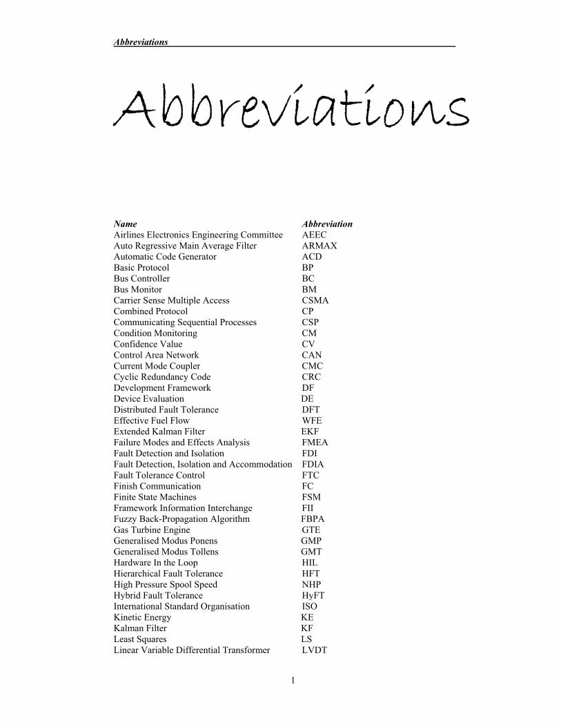
Abbreviations
Name Abbreviation Airlines Electronics Engineering Committee AEEC Auto Regressive Main Average Filter ARMAXAutomatic Code Generator ACD Basic Protocol BP Bus Controller BC Bus Monitor BM Carrier Sense Multiple Access CSMA Combined Protocol CP Communicating Sequential Processes CSP Condition Monitoring CM Confidence Value CV Control Area Network CAN Current Mode Coupler CMCCyclic Redundancy Code CRC Development Framework DF Device Evaluation DE Distributed Fault Tolerance DFT Effective Fuel Flow WFE Extended Kalman Filter EKF Failure Modes and Effects Analysis FMEA Fault Detection and Isolation FDI Fault Detection, Isolation and Accommodation FDIA Fault Tolerance Control FTC Finish Communication FC Finite State Machines FSM Framework Information Interchange FII Fuzzy Back-Propagation Algorithm FBPA Gas Turbine Engine GTE Generalised Modus Ponens GMP Generalised Modus Tollens GMT Hardware In the Loop HIL Hierarchical Fault Tolerance HFT High Pressure Spool Speed NHP Hybrid Fault Tolerance HyFTInternational Standard Organisation ISO Kinetic Energy KE Kalman Filter KF Least Squares LS Linear Variable Differential Transformer LVDT
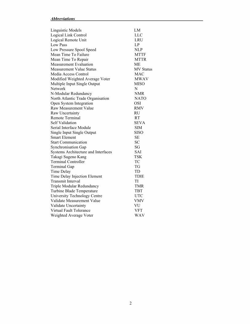
Abbreviations
2
Linguistic Models LM Logical Link Control LLC Logical Remote Unit LRU Low Pass LP Low Pressure Spool Speed NLP Mean Time To Failure MTTF Mean Time To Repair MTTR Measurement Evaluation ME Measurement Value Status MV Status Media Access Control MAC Modified Weighted Average Voter MWAV Multiple Input Single Output MISO Network N N-Modular Redundancy NMRNorth Atlantic Trade Organisation NATO Open System Integration OSI Raw Measurement Value RMV Raw Uncertainty RU Remote Terminal RT Self Validation SEVA Serial Interface Module SIM Single Input Single Output SISO Smart Element SE Start Communication SC Synchronisation Gap SGSystems Architecture and Interfaces SAI Takagi Sugeno Kang TSK Terminal Controller TC Terminal Gap TG Time Delay TD Time Delay Injection Element TDIE Transmit Interval TI Triple Modular Redundancy TMR Turbine Blade Temperature TBT University Technology Centre UTC Validate Measurement Value VMV Validate Uncertainty VU Virtual Fault Tolerance VFT Weighted Average Voter WAV

Chapter 1 Introduction
3
Introduction The aim of this thesis is the study of “Smart” Distributed Systems. This leads to several
important research areas. Firstly, with heterogeneous architectures one must consider the
diverse processing resources and also the impact of communication via a databus. When
considering fault tolerant strategies, such as Analytical Redundancy, the performance of the
system must be evaluated for a number of non-faulty and faulty scenarios. The thesis thus
addresses these areas building upon key elements gradually integrating these into a
heterogeneous distributed system based upon Control Area Network databus (CANbus).
Fig. 1.1 shows the stages of development in this thesis. Firstly, the concept of “smart”
elements is introduced, where a “smart” element can be a sensor/actuator with in-built
processing or an intelligent module. Secondly, Fault Detection and Isolation (FDI) techniques
are defined and evaluated for “smart” elements. These are then integrated within a distributed
system. For this, the impact of databus communication is considered in detail. The diagnostic
information generated by the “smart” elements within the system is then used within a
number of different fault accommodation strategies. Finally, the performance of the overall
system is evaluated.
Evaluation ofPerformanceDegradation
Evaluation ofFDI
Evaluation ofSmart
Techniques
FDI
FaultAccommodation
DistributedSystems
SmartElements
Evaluation ofCommunication
Systems
Design Comparison
Fig. 1.1 Strategy followed during the design of this research
Chapter 1 Introduction
4
At each development stage, feedback of design experience is used to optimise the overall
system concept. In addition, to practically demonstrate the ideas developed in this thesis a
case study has been performed within the Rolls-Royce University Technology Centre for
Control and Systems at the University of Sheffield. This consists of a real-time distributed
system demonstrator of a gas turbine engine controller using “smart” sensors and actuators.
The engine is a multiple input multiple output system. The associated controller is a multiple
input single output system controlling the main engine fuel valve. A full explanation of this
model is given in Chapter 5.
The thesis has a number of aims. Firstly, several techniques are developed to implement
“smart” elements (sensors and actuators) capable of detecting faults, such as, noise, drift etc.
Thus, fault injection, estimation procedures and evaluation procedures are studied. An
important issue is definition of a standard format for information generated by “smart”
elements. In this work the Self Validating (SEVA) standard developed for process control has
been extended for this safety-critical application.
A second objective is to define fault tolerance strategies for distributed systems. Initially,
these approaches must focus on the local faults detected by the “smart” elements. These
methodologies are based upon a temporal behaviour due to the synchronous and immediate
response needed with respect to the faulty element. Hence, their definition is established in
terms of finite state machines and their evaluation is performed by the temporal impact that
they have on the distributed system.
It is important to develop a model of a distributed system in order to analyse the effects of
time delays. Therefore, a model was developed which simulates and calculates the time
delays for the communication between elements within a distributed system. This model also
considers the impact of faults which may occur in the system. The resultant delay times are
then injected into a dynamic simulation of the gas turbine engine and controller in closed-
loop. This allows evaluation of the degradation in performance of the control system for
different fault scenarios.
Leading on from the distributed system modelling a real-time hardware-in-the-loop (HIL)
implementation was used to validate the results obtained previously. A distributed system was
constructed using CANbus. This system consists of three nodes, the engine, the controller and
a “smart” actuator (stepper motor with feedback sensor). A number of fault tolerance
strategies were implemented on this hardware demonstrator and the real-time performance
was evaluated for injected faults.
Chapter 1 Introduction
5
The thesis is divided into seven chapters. In this first chapter an overview of the work is
given. In the second chapter an introduction is given to distributed systems, fault tolerance
and “smart” elements. Chapter three details the theoretical implementation of “smart” sensors
and actuators. In Chapter four a “smart” sensor and actuator are implemented and results are
given for a number of injected faults. Chapter five concentrates on fault tolerance approaches
for a distributed system. Chapter six brings together the concepts developed through the
implementation of a real-time HIL gas turbine engine controller demonstrator. Finally,
Chapter seven highlights the most important points and results obtained in this investigation.
In addition, avenues for further work are discussed.

Chapter 2 Background
6
Chapter 2 2.1 INTRODUCTION
In this chapter the main concepts of distributed systems and fault tolerance are introduced.
Firstly, distributed systems are explained in terms of the open system interconnection (OSI-7)
layer model. This model allows the division of the system into layers of embedded
functionality. Within this framework “smart” elements are introduced. The importance of
system synchronisation and data consistency is highlighted. An important consideration for
the application in this work (an aerospace gas turbine engine) is the databus standard used for
interconnection. A number of common aerospace databuses are introduced. It is highlighted
that these are not appropriate for this particular application, hence, the Control Area Network
(CAN) standard is proposed. This databus offers a number of advantages: low cost, suitable
bandwidth, low protocol overhead and message prioritisation. The CANbus is used later as
the basis of the distributed system demonstrator described in Chapter 6.
In the second part of this Chapter, the basic approaches to fault tolerance are introduced.
Firstly, definitions of different fault types are made. This is followed by a description of
techniques for fault detection, isolation and accommodation (FDIA). A number of possible
evaluation measures are discussed in order to define a framework for describing system
performance. Finally, a summary is given.
2.2 DISTRIBUTED SYSTEMS
There are several ways of defining distributed systems, from a formal definition, to a
methodology of implementation (Zomaya, 1996). However, a general definition is: “a
distributed system is formed by a group of processors sharing a communication media for a
global task”.
This first section is divided into three main areas. In the first part a formal interpretation of
distributed systems based upon the OSI model is presented. In the second part the concept of

Chapter 2 Background
7
“smart” elements is introduced. This is central to this research work. The third part discusses
data synchronisation and data consistency in distributed systems.
2.2.1 The OSI 7 Layer Model
A distributed system is one in which several autonomous processors and data stores
supporting processes and/or databases interact in order to cooperate and achieve an overall
goal. The processes co-ordinate their activities and exchange information by means of
information transferred over a communication network (Sloman et al., 1987). One of the basic
characteristics of distributed systems is that interprocess messages are subject to variable
delays and failure. There is a defined time between occurrence of an event and its availability
for observation at some other point.
The simplest view of the structure of a distributed system is that it consists of a set of
physically distributed computer stations interconnected by some communications network.
Each station has the capability for processing and storing data, and may have connections to
external devices. Table 2.1 is a summary to provide an impression of the functions performed
by each layer in a typical distributed system (Sloman et al., 1987). It is important to highlight
that this is just a first attempt in order to define an overall formal concept of the OSI layer.
Layer Example Application software Monitoring and control modules Utilities File transfer, device handlers Local management Software process management Kernel Multitasking, I/O drivers, memory
management Hardware Processors, memory I/O devices Communication system Virtual circuits, network routing, flow control
error control Table 2.1 OSI Layer non-formal attempt
This local layered structure is the first attempt in understanding how a distributed system is
constructed. It provides a basis for describing the functions performed and services offered at
a station. The basic idea of layering is that, regardless of station boundaries, each layer adds
value to the services provided by the set of lower layers. Viewed from above, a particular
layer and the ones below it may be considered to be a ‘black box’ which implements a set of
functions in order to provide a service. A protocol is the set of rules governing
communication between the entities, which constitute a particular layer. An interface between
two layers defines the means by which one local layer makes use of services provided by the
lower layer. It defines the rules and formats for exchanging information across the boundary
between adjacent layers within a single station.
Chapter 2 Background
8
The communication system at a station is responsible for transporting system and application
messages to/from that station. It accepts messages from the station software, and prepares
them for transmission via a shared network interface. It also receives messages from the
network and prepares them for receipt by the station software.
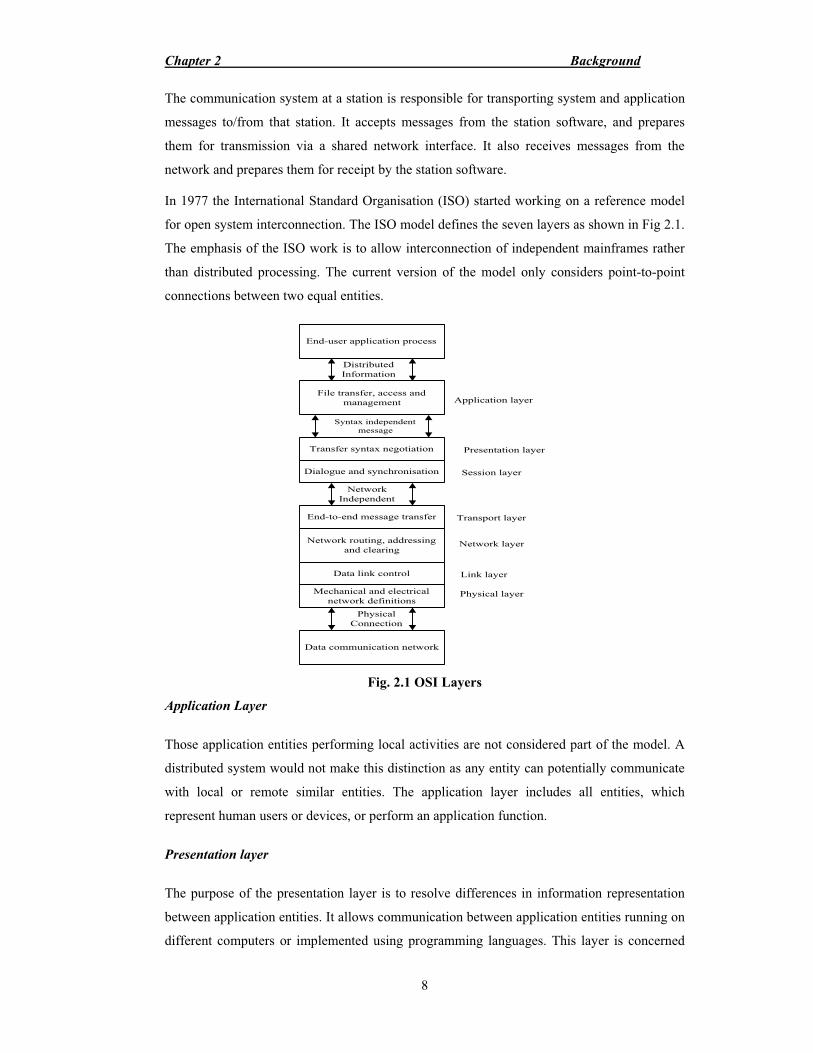
In 1977 the International Standard Organisation (ISO) started working on a reference model
for open system interconnection. The ISO model defines the seven layers as shown in Fig 2.1.
The emphasis of the ISO work is to allow interconnection of independent mainframes rather
than distributed processing. The current version of the model only considers point-to-point
connections between two equal entities.
End-user application process
File transfer, access andmanagement
Transfer syntax negotiation
Data communication network
Dialogue and synchronisation
End-to-end message transfer
Network routing, addressingand clearing
Data link control
Mechanical and electricalnetwork definitions
Application layer
Presentation layer
Session layer
Transport layer
Network layer
Link layer
Physical layer
DistributedInformation
NetworkIndependent
Syntax independentmessage
PhysicalConnection
Fig. 2.1 OSI Layers
Application Layer
Those application entities performing local activities are not considered part of the model. A
distributed system would not make this distinction as any entity can potentially communicate
with local or remote similar entities. The application layer includes all entities, which
represent human users or devices, or perform an application function.
Presentation layer
The purpose of the presentation layer is to resolve differences in information representation
between application entities. It allows communication between application entities running on
different computers or implemented using programming languages. This layer is concerned

Chapter 2 Background
9
with data transformation, formatting, structuring, encryption and compression. Many of these
functions are application dependent and are often performed by high-level language
compilers, so the borderline between presentation and application layers is not clear.
Session layer
This layer provides the facilities to support and maintain sessions between application
entities. Sessions may extend over a long time interval involving many message interactions
or be very short involving one or two messages.
Transport layer
The transport layer is the boundary between what are considered the application-oriented
layers and the communication-oriented layer. This is the lowest layer using an end-station-to-
end-station protocol. It isolates higher layers from concerns such as how reliable and cost-
effective transfer of data is actually achieved. The transport layers usually provide
multiplexing; end-to-end error and flow control, fragmenting and reassembly of large
messages into network packets and mapping of transport-layer identifiers onto network
addresses.
Network layer
The network layer isolates the higher layers from routing and switching considerations. The
network layer masks the transport layer from all the peculiarities of the actual transfer
medium: whether a point-to-point link, packet switched network, LAN or even interconnected
networks. It is the network layer’s responsibility to get a message from a source station to the
destination station across an arbitrary network topology.
Data-link layer
The task of this layer is to take the raw physical circuit and convert it into a point-to-point link
that appears relatively error free to the network layer. It usually entails error and flow control
but many local area networks have low intrinsic error rates and so do not include error
correction.
Physical layer
This layer is concerned with transmission of bits over a physical circuit. It performs all
functions associated with signalling, modulation and bit synchronisation. It may perform error
detection by signal quality monitoring.
Chapter 2 Background
10
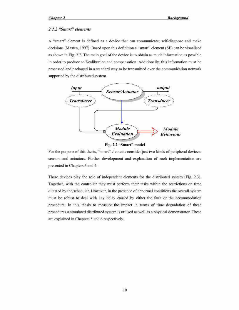
2.2.2 “Smart” elements
A “smart” element is defined as a device that can communicate, self-diagnose and make
decisions (Masten, 1997). Based upon this definition a “smart” element (SE) can be visualised
as shown in Fig. 2.2. The main goal of the device is to obtain as much information as possible
in order to produce self-calibration and compensation. Additionally, this information must be
processed and packaged in a standard way to be transmitted over the communication network
supported by the distributed system.
Sensor/Actuatorinput output
ModuleEvaluation
Transducer Transducer
ModuleBehaviour
Fig. 2.2 “Smart” model
For the purpose of this thesis, “smart” elements consider just two kinds of peripheral devices:
sensors and actuators. Further development and explanation of each implementation are
presented in Chapters 3 and 4.
These devices play the role of independent elements for the distributed system (Fig. 2.3).
Together, with the controller they must perform their tasks within the restrictions on time
dictated by the scheduler. However, in the presence of abnormal conditions the overall system
must be robust to deal with any delay caused by either the fault or the accommodation
procedure. In this thesis to measure the impact in terms of time degradation of these
procedures a simulated distributed system is utilised as well as a physical demonstrator. These
are explained in Chapters 5 and 6 respectively.

Chapter 2 Background
11
"Smart" Sensor
"Smart"Actuator
ControllerPlant"Smart" Sensor
Fault ToleranceModule
External Fault Tolerance
Module
Fig. 2.3 Network Concept
Fig. 2.3 shows different approaches to “smart” sensors combined with local fault tolerance
strategies. A “smart” sensor may rely on an external module for fault tolerance or it may have
in-built fault tolerance. Similarly, actuators may adopt either of these approaches.
2.2.3 System Synchronisation and Data Consistency
It is very important in a distributed system to ensure system synchronisation. Without tight
synchronisation it is likely that the system will lose data consistency. For example, sensors
may be sampled at different times leading to failures being detected due to differences
between data values. It is also important to consider intermediate data and consistency
between replicated processing if comparison/voting is used to avoid the states of the replicas
from diverging (Brasileiro et al., 1995). Asynchronous events and processing of non-identical
messages could both lead to replica state divergence. Synchronisation at the level of processor
micro-instructions is logically the most straightforward way to achieve replica synchronism.
In this approach, processors are driven by a common clock source, which guarantees that they
execute the same step at each clock pulse. Outputs are evaluated by a (possibly replicated)
hardware component at appropriate times. Asynchronous events must be distributed to the
processors of a node through special circuits which ensure that all the correct processors will
perceive such an event at the same point of their instruction flow. Since every correct
processor of a node executes the same instruction flow, all the programs that run on the non-
redundant version can be made to run, without any changes, on the node (as concurrent
execution). There are, however, a few problems with the micro-instruction level approach to
synchronisation. Firstly, as indicated before, individual processors must be built in such a way
that they will have a deterministic behaviour at each clock pulse. Therefore, they will produce
Chapter 2 Background
12
identical outputs. Secondly, the introduction of special circuits such as a reliable
comparator/voter, a reliable clock, asynchronous event handlers, and bus interfaces, increases
the complexity of the design, which in the extreme can lead to a reduction in the overall
reliability of a node. Thirdly, every new microprocessor architecture requires a considerable
re-design effort. Finally, because of their tight synchronisation, a transient fault is likely to
affect the processors in an identical manner, thus making a node susceptible to common mode
failures.
An alternative approach that tries to reduce the hardware level complexity associated with the
approaches discussed above is to maintain replica synchronism at a higher level, for instance
at the process, or task level by making use of appropriate software implemented-protocols.
Such software-implemented nodes can offer several advantages over their hardware-
implemented equivalents:
� Technology upgrades appear to be easy; since the principles behind the protocols do not
change.
� Employing different types of processors within a node, there is a possibility that a
measure of tolerance against design faults in processors can be obtained, without recourse
to any specialised hardware.
Fail silent nodes are implemented at the higher software fault tolerance layer. The main goal
is to detect faults inside of a number of processors (initially two) that compose a node. As
soon as one of the processors has detected a fault it has two options; either remain fail silent
or decrease its own performance. The latter option is suitable when the faulty processor is still
checking information from the other processor. This implementation involves: firstly, a
synchronisation technique called “order protocol” and secondly, a comparison procedure that
validates and transmits the information or remains silent if there is a fault. The concept used
for local fault tolerance in fail silent nodes is the basis of the approach followed in this thesis
for the “smart” elements. However, in this case, in the presence of a fault the nodes should not
remain silent.
The main advantage of fail silent nodes is the use of object oriented programming for
synchronisation protocols to allow comparison of results from both processors at the same
time. Fail silent nodes within fault tolerance are considered to be the first move towards
mobile objects (Caughey et al., 1995). Although the latter technique is not explained here, it
remains an interesting research area for fault tolerance.

Chapter 2 Background
13
System model and assumptions. It is necessary to assume that the computation performed by
a process on a selected message is deterministic. This is the well-known assumption in state
machine models for which the precise requirements for supporting replicated processing are
known (Schneider, 1990). Basically, in the replicated version of a process, multiple input
ports of the non-replicated process are merged into a single port and the replica selects the
message at the head of its port queue for processing. So, if all the non-faulty replicas have
identical states then they produce identical output messages. Having provided the queues with
all correct replicas, they can be guaranteed to contain identical messages in identical order.
Thus, replication of a process requires the following two conditions to be met:
Agreement: all the non-faulty replicas of a process receive identical input messages.
Order: all the non-faulty replicas process the messages in an identical order.
Practical distributed programs often require some additional functionality such as using time-
outs when they are waiting for messages. Time-outs and other asynchronous events, such as
high priority messages, etc. are potential sources of non-determinism during input message
selection, making such programs difficult to replicate. Further on (Chapter 6), this non-
determinism is handled as an inherent characteristic of the system.
It is assumed that each processor of a fail-silent node has network interfaces for inter-node
communication over networks. In addition, the processors of a node are internally connected
by communication links for intra-node communication needed for the execution of the
redundancy management protocols. The maximum intra-node communication delay over a
link is known and bounded. If a non-faulty process of a neighbour processor sends a message,
then the message will be received within � time units. Communication channel failures will
be categorised as processor failures.
2.2.4 Databuses
For the gas turbine engine controller application it was first necessary to consider the databus
standard to be used on-engine for the distributed system. There are a number of standards
used in aerospace. In the following sections the most common databuses are introduced.
ARINC 429
The ARINC 429 databus is a digital broadcast databus developed by the Airlines Electronics
Engineering Committee’s (AEEC) and Systems Architecture and Interfaces (SAI). The
Chapter 2 Background
14
AEEC, which is sponsored by ARINC, released the first publication of the ARINC
specification 429 in 1978.
The ARINC 429 databus (Avionics Communication, 1995) is a unidirectional type bus with
only one transmitter. Transmission contention is thus not an issue. Another factor contributing
to the simplicity of this protocol is that it was originally designed to handle “open loop” data
transmission. In this mode, there is no required response from the receiver when it accepts a
transmission from the sender. This databus uses a word length of 32 bits and two transmission
rates: low speed, which is defined as being in the range of 12 to 14.5 Kbits/s consistency with
units for 1553b (Freer, 1989); and high speed which is 100 Kbits/s.
There are two modes of operation in the ARINC 429 bus protocol: character oriented mode
and bit-oriented mode. Since the ARINC 429 bus is a broadcast bus, the transmitter on the bus
uses no access protocols. Out of the 32-bit word length used, a typical usage of the bits would
be as follows:
� Eight bits for the label
� Two bits for the source /Destination Identifier
� Twenty-one data bits
� One parity bit
This databus has the advantage of simplicity, however, if the user needs more complicated
protocols or it is necessary to use a very complicated communication structure, the data
bandwidth is used rapidly.
One of the characteristics used by ARINC 429 is the LRU (Logical Remote Unit) to verify
that the number of words expected match with those received. If the number of words does
not match the expected number, the receiver notifies the transmitter within a specific amount
of time.
Parity checks use one bit of the 32-bit ARINC 429 data word. Odd parity was chosen as the
accepted scheme for ARINC 429 compatible LRU’s. If a receiving LRU detects odd parity in
a data word, it continues to process that word. If the LRU detects even parity, it ignores the
data word.
Chapter 2 Background
15
ARINC 629
ARINC 629-2 (1991) has a speed of 2 MHz with two basic modes of protocol operation. One
is the Basic Protocol (BP), where transmissions may be periodic or aperiodic. Transmission
lengths are fairly constant but can vary somewhat without causing aperiodic operation if
sufficient overhead is allowed. In the Combined Protocol (CP) mode transmissions are
divided into three groups of scheduling:
� Level 1 is periodic data (highest priority)
� Level 2 is aperiodic data (mid-priority)
� Level 3 is aperiodic data (lowest priority)
In level one data is sent first, followed by level two and level three. Periodic data is sent in
level one in a continuous stream until finished. Afterwards, there should be time available for
transmission of aperiodic data. The operation of transferring data from one LRU to one or
more other LRU’s occurs as follows:
1. The Terminal Controller (TC) retrieves 16-bit parallel data from the transmitting LRU’s
memory.
2. The TC determines when to transmit, attaches the data to a label, converts the parallel
data to serial data and sends it to the Serial Interface Module (SIM).
3. The SIM converts the digital serial data into an analogue signal and sends them to the
current mode coupler (CMC) via the stub (twisted pair cable).
4. The CMC inductively couples the doublets onto the bus. At this point, the data is
available to all other couplers on the bus.
This protocol has three conditions, which must be satisfied for proper operation: the
occurrence of a Transmit Interval (TI), the occurrence of a Synchronisation Gap (SG), and the
occurrence of a TG (Terminal Gap). The TI defines the minimum period that a user must wait
to access the bus. It is set to the same value for all users. In the periodic mode, it defines the
update rate of every bus user. The SG is also set to the same value for all users and is defined
as a bus quiet time greater than the largest TG value. Every user is guaranteed bus access once
every TI period. The TG is a bus quiet time, which corresponds to the unique address of a bus
user. Once the number of users is known, the range of TG values can be assigned and the SG
and TI values determined. TI is given by the following table.

Chapter 2 Background
16
Binary Value (BV) BV TI (ms) TG (micro seconds)TI6 TI5 TI4 TI3 TI2 TI1 TI0 0 0 0 0 0 0 0 0 0.5005625 not used 0 0 0 0 0 0 1 1 1.0005625 not used ... ... ... ... ... ... ... ... ... ... 1 1 1 1 1 1 1 126 64.0005625 127.6875
Table 2.2 ARINC 629 time characteristics
To program the desired TG for each node, the user must follow Table 2.2 from TI6 to TI0
which represent the binary value (BV).
MIL-STD 1553b
Another commonly used databus is MIL-STD 1553b (Freer, 1989). This is a serial, time
division multiplexed databus using screened twisted-pair cable to transmit data at 1Mbit/s.
Data is transmitted in 16-bit words with a parity and a 3-bit period synchronisation signal,
with a whole word taking 20 microseconds to be transmitted. Transformer-coupled base-band
signalling with Manchester encoding is employed. Three types of devices may be attached to
the databus:
� Bus Controller (BC)
� Remote Terminal (RT)
� Bus Monitor (BM)
The use of MIL-STD-1553b in military aircraft has simplified the specification of interfaces
between avionics subsystems and goes a long way towards producing off-the-shelf
interoperability.
Most avionics applications of this databus require a duplicated, redundant bus cable and bus
controller to ensure continued system operation in case of a single bus or controller failure.
MIL-STD-1553b is intended primarily for systems with central intelligence and intelligent
terminals in applications where the data flow patterns are predictable.
Information flow on the databus includes messages, which are formed from three types of
words (command, data and status). The maximum amount of data which may be contained in
a message is 32 data words, each word containing sixteen data bits, one parity bit and three
synchronisation bits.
The bus controller only sends command words, their content and sequence determine which
of the four possible data transfers must be undertaken:

Chapter 2 Background
17
� Point-to-Point between controller and remote terminal
� Point-to-Point between remote terminals
� Broadcast from controller
� Broadcast from a remote terminal
There are six formats for point-to-point transmissions:
� Controller to RT data transfer
� RT to controller data transfer
� RT to RT data transfer
� Mode command without a data word
� Mode command with data transmission
� Mode command with data word reception
and four broadcast transmission formats are specified:
� Controller to RT data transfer
� RT to RT(s) data transfer
� Mode command without a data word
� Mode command with a data word
This databus incorporates two main features for safety-critical systems, a predictable
behaviour based upon its pooling protocol and the use of bus controllers. They permit
communication handling to avoid collisions on the databus. MIL-STD-1553b also defines a
procedure for issuing a bus control transfer to the next potential bus controller which can
accept or reject control by using a bit in the returning status word.
From this information it can be concluded that MIL-STD 1553b is a very flexible data bus. A
drawback, however, is that the use of a centralised bus controller reduces transmission speed
as well as reliability.

Chapter 2 Background
18
2.2.5 Databus Selected for Demonstrator
In Chapter 5 (see Section 5.4) a comparison of these databuses is made leading to the
conclusion that they are all unsuitable for this application. Hence, this section also introduces
the CAN databus which was originally developed for automotive applications. This is suitable
for this application and therefore is used as the basis of the demonstrator explained in Chapter
6.
CAN (Control Area Network) databus
CANbus (ISO DIS 11898, 1992), is a communication databus designed for sending and
receiving short real-time control messages. CAN is a broadcast databus where a number of
processors are connected to the bus via an interface. A data source is transmitted as a
message, consisting of between 1 and 8 bytes (‘octets’). A data source may be transmitted
periodically, sporadically, or on demand. The data source is assigned a unique identifier,
represented as an 11-bit number giving 2032 identifiers (CAN prohibits identifiers with the
seven most significant bits equal to ‘1’). The identifier serves two purposes: filtering
messages upon reception and assigning a priority to the message (Tindell et al., 1995).
A station on a CANbus is able to receive a message based on the message identifier. Thus in
CAN a message has no destination. The identification also gives the priority of the message.
CAN is a carrier-sense broadcast bus, but takes a much more systematic approach to
contention. The identifier field of a CAN message is used to control access to the bus after
collisions by taking advantage of certain electrical characteristics. For example, if multiple
stations are transmitting concurrently and one station transmits a ‘0’ bit then all stations
monitoring the bus will see a ‘0’. Conversely, only if all stations transmit a ‘1’ will all
processors monitoring the bus see a ‘1’. In CAN terminology, a ‘0’ bit is termed dominant
and a ‘1’ bit is termed recessive. In effect, the CANbus acts like a large AND-gate, with each
station able to see the output of the gate. This behaviour is used to resolve collisions. The
following arbitration sequence is used:
� Firstly, each station waits until bus idle. When silence is detected each station begins to
transmit the highest priority message held in its queue whilst monitoring the bus. The
message is coded so that the most significant bit of the identifier field is transmitted first.
� If a station transmits a recessive bit, but monitors a dominant bit then a collision is
detected. The station knows that the message it is transmitting is not the highest priority
message in the system, stops transmitting, and waits for the bus to become idle.

Chapter 2 Background
19
� If the station transmits a recessive bit and sees a recessive bit on the bus, then it may be
transmitting the highest priority message. It therefore, proceeds to transmit the next bit of
the identifier field.
CAN requires identifiers to be unique within the system (per message). A station transmitting
the last bit (least significant bit) of the identifier without detecting a collision must be
transmitting the highest priority queued message and hence can start transmitting the body of
the message. CAN, in fact, can resolve in a deterministic way any collision which could take
place on the shared bus. When a collision occurs an arbitration procedure is set off which
immediately stops all the transmitting stations, except for that one which is sending the object
with the lowest numerical identifier (highest priority).
There are some general observations to make on this arbitration protocol. Firstly, a message
with a smaller identifier value is a higher priority message. Secondly, the highest priority
message undergoes the arbitration process without disturbance. The whole message is
transmitted without interruption.
One of the perceived problems of CAN is the inability to bound the response times messages.
From the observations above, the worst-case time from queuing the highest priority message
to the reception of that message can be calculated easily. The longest time a station must wait
for the bus to become idle is the longest time to transmit a CAN message. According to
Tindell et al., (1995) the largest CAN message (8 bytes) takes 130 microseconds to be
transmitted. For a lower priority message, the worst-case response time cannot be found so
easily. A message waits for highest priority message to be serviced first.
CAN is a particular class of Carrier Sense Multiple Access (CSMA) network which, unlike
the traditional carrier sense multiple access with collision detection (CSMA/CD) network
(ISO/IS, 1985), enforces a clear medium access policy based on the priority of the exchanged
objects.
The CAN specification (ISO 11898) discusses only the physical and data-link layer for a
CAN network:
� The Data Link Layer is the only layer that recognises and understands the format of
messages. This layer constructs the messages to be sent to the Physical Layer, and
decodes messages received from the Physical Layer. In CAN controllers, the Data Link

Chapter 2 Background
20
Layer is usually implemented in hardware. Because of its complexity and in common
with most other networks this is divided into a:
� Logical Link Control (LLC) layer which handles transmission and reception of
data messages to and from other, higher level layers in the model.
� Media Access Control (MAC) layer, which encodes and serialises messages for
transmission and decodes received messages. The MAC also handles message
prioritisation (arbitration), error detection and access to the Physical Layer.
� The Physical Layer specifies the physical and electrical characteristics of the bus. This
includes the hardware that converts the characters of a message into electrical signals for
transmitted messages and likewise the electrical signals into characters for received
messages.
At first impression CANbus appears to be an unpredictable and non-deterministic databus.
This supposition can be avoided, if each identifier is considered as a priority level per
message transmitted. As the identifier number increases the priority of the message decreases.
This is an inherent property of CANbus, that can be used for predictability if each message is
related to a task in the system. For instance, a very high priority task such as a real-time clock
may need to be transmitted ahead of other critical tasks (Lawrenz, 1997). Synchronisation is
one of the main issues which needs to be addressed with CANbus. This is discussed in
Chapter 6 where CANbus is used to develop the fault tolerant distributed demonstrator.
2.3 FAULT TOLERANCE CONCEPTS
Fault Tolerance (Johnson, 1989) is an attribute that is designed into a system to achieve a
design goal. Just as a design must meet many functional and performance goals, it must
satisfy numerous other requirements as well. In the following sections, a short explanation of
concepts considered by the author as basic for the study of fault tolerance is given.
The following definitions are taken from fault characteristics defined by Johnson (1989). A
fault is a defect or imperfection in the physical implementation that occurs within some
hardware or software component. An error is a manifestation of a fault deviation from
accuracy or correctness. If the error results in the system performing one of its functions
incorrectly, a system failure has occurred. Hence, a failure is the non-performance of some
action that is due or expected. The fault duration specifies the quantity of time that a fault is
active. A fault can be permanent when it remains in existence indefinitely if no corrective
action is taken, a fault can be transient where it can appear and disappear within a very short
Chapter 2 Background
21
period of time, or it can be intermittent where it appears, disappears, and then reappears
repeatedly. The fault extent specifies whether the fault is localised to a given hardware or
software module or whether it globally affects the hardware, the software, or both. The fault
value can be either determinate or indeterminate. A determinate fault is one whose status
remains unchanged throughout time unless externally acted upon. An indeterminate fault is
one whose status at some time T may be different from its status at some other time. A
complementary definition of faults related to the dynamics of the system is explained in
Chapter 3.
2.3.1 Fault Detection and Isolation Techniques (FDI)
In this section an overview of different fault tolerant techniques is given to show the diversity
of methodologies which can be used.
Fault avoidance is any technique that is used to prevent faults in the first place. Fault
avoidance can include several techniques such as design reviews, component screening,
testing and other quality methods. Fault tolerance is the ability of a system to continue to
perform its tasks after the occurrence of faults. Fault tolerance can be achieved using a
number of techniques. For instance, fault masking is one approach. Fault masking is any
process that prevents faults in a system from introducing errors into the structure of that
system. Another approach is to detect and locate the fault that has occurred and reconfigure
the system to remove the faulty component. Reconfiguration is the process of eliminating a
faulty entity from a system and restoring the system to some operational condition or state. If
a reconfiguration technique is used, the designer must consider the following processes:
� Fault Detection
� Fault Location
� Fault Recovery
Due to the increasing complexity of modern control systems, fault tolerance becomes an issue
of high priority. This can be achieved by either passive or active strategies. The first approach
makes use of robust strategies in order to make the process insensitive (Frank, 1996).
Alternatively, the active approach provides fault accommodation through reconfiguration of
the system. For the latter strategy a number of tasks have to be performed:
� Fault Detection,
� Fault Isolation and

Chapter 2 Background
22
� Fault Analysis.
In this section the first two techniques are considered for the detection of time of the fault and
its localisation (classification).
Further on (Chapters 3 and 4), analytical model-based techniques are used to assess the
degradation of the “smart” elements in the presence of faults.
2.3.2 Redundancy Techniques
All fault tolerance techniques use some form of hardware and/or software redundancy. Fault
tolerance can utilise hardware, software and information redundancy. Its integration into
different systems depends on their particular application characteristics. Although the main
fault tolerant goal remains the same, there are several strategies for implementation:
� Migration of processes
� Physical reconfiguration
� More reliable components
� Voting (continuous and hybrid)
� Hierarchical fault tolerance
� Distributed fault tolerance
The most common technique used to achieve some form of fault tolerance is the physical
replication of boxes or hardware components within a system (Johnson, 1984). Redundancy
is simply the addition of information, resources, or time beyond that needed for formal system
operation. The redundancy can take one of several forms (Johnson, 1989):
� Hardware redundancy is the addition of extra hardware, usually for the purpose of
either detecting or tolerating faults. There are three basic forms of hardware redundancy:
passive, active, and hybrid. Passive techniques use the concept of fault masking to hide
the occurrence of faults and prevent the faults from resulting in errors. Passive approaches
are designed to achieve fault tolerance without requiring any action on the part of the
system or an operator. Passive techniques, in their most basic form, mask faults rather
than detect them (for example voters).

Chapter 2 Background
23
The most common form of passive hardware redundancy is called Triple Modular
Redundancy (TMR). The basic concept of TMR is to triplicate the hardware and perform
a majority vote to determine the output of the system. If one of the modules becomes
faulty, the two remaining fault-free modules mask the results of the faulty module when
the majority vote is performed. The primary difficulty with TMR is the voter; if the voter
fails, the complete system fails. In other words, the reliability of the simplest form of
TMR can be no better than the reliability of the voter. Any single component within a
system whose failure leads to a failure of the system is called a single point of failure. A
generalisation of the TMR approach is the N-modular redundancy (NMR) technique.
NMR applies the same principle as TMR but uses N of a given module as opposed to only
three. In most cases, N is selected as an odd number so that a majority voting arrangement
can be used. The primary trade-off in NMR is the fault tolerance achieved versus the
hardware required. Further information about TMR voting is described in Chapter 5.
The active approach, which is sometimes called the dynamic method, achieves fault
tolerance by detecting the existence of faults and performing some action to remove the
faulty hardware from the system. Active hardware redundancy uses fault detection, fault
location and fault recovery to achieve fault tolerance. This procedure is named Fault
Detection, Isolation and Accommodation (FDIA). Software fault tolerance through
migration objects like intelligent agents or fail silent nodes are typical implementations.
Hybrid techniques combine the most important characteristics of both the passive and
active approaches. Fault masking is used in hybrid systems to prevent erroneous results
from being propagated. FDIA is also used in the hybrid approaches to improve fault
tolerance by masking faulty hardware with spares. Hybrid methods are often used in
critical computation applications where fault masking is required to prevent momentary
errors, and high reliability must be achieved. A typical example is the combination of
“smart” elements and voters to increase the reliability of the whole group, although,
different voter types can provide a very robust scheme. Further explanation is provided in
Chapter 5.
� Software Redundancy is the addition of extra software, beyond that needed to perform a
given function to detect and possibly tolerate faults. Programming techniques such as
object oriented techniques become useful to define reliable procedures for fault tolerance
(Jalote, 1994). An example of this technique is explained by Beedubail et al., (1996).
� Information Redundancy is the addition of extra information beyond that required for
implementing a given function; for example, error detection codes use a form of

Chapter 2 Background
24
information redundancy. Within distributed systems it is necessary to define a
communication protocol. This cannot be considered 100% fault free. Therefore,
information coding is required to detect errors.
Coding is one of the most important techniques for supporting fault tolerance in hardware.
It is also used extensively for improving the reliability of communication. The basic idea
behind coding is to add check bits to the information bits such that errors in some bits can
be detected, and if possible, corrected. The process of adding check bits to information
bits is called encoding. The reverse process of extracting information from the encoded
data is called decoding. Hence, coding essentially provides structural checks, in which the
error is detected by detecting inconsistency in the structural integrity of the data. Different
forms of coding exist such as:
1. Hamming Codes
2. Cyclic Redundancy Codes
3. Berger Codes
4. Residue Codes
These techniques are not studied in this thesis but could be applied to the communication
in the CANbus demonstrator.
� Time Redundancy uses additional time to perform the functions of a system such that
fault detection and fault tolerance can be achieved. The basic concept of time redundancy
is the repetition of communication in ways that allow faults to be detected. Time
redundancy can function in a system in several ways, but the most basic form of time
redundancy is to perform a software block two or more times and compare the results to
determine if a discrepancy exists. If an error is detected, the computation can be
performed again to see if the disagreement remains or disappears. Such approaches are
often good for detecting errors resulting from transient faults, but they cannot protect
against errors resulting from permanent faults.
Reconfiguration or other action, like physical redundancy, within the control system in
reaction to a fault is referred to as fault accommodation. Specific actions are required to
accommodate faults detected in a system, based upon the application considered. Required
operation can be one or more of the items listed below:
� Change performance:

Chapter 2 Background
25
� Decrease performance.
� Change settings in the surrounding process to decrease the requirements of the
controlled system.
� Change controller parameters.
� Reconfigure:
� Use component redundancy if possible.
� Change controller structure.
� Replace a sensor with signal estimator/observer. Note this operation may be
limited in time because external disturbances may increase the estimation error.
� If the fault is a set point error then freeze the system at last fault-free set point and
continue control operation. Issue an alert message to operators.
� Stop operation:
� Freeze controller output to a predetermined value. Three commonly required
values are Zero, maximum or the last fault-free value. The one to be used is
entirely application dependent.
� Fail-to-safe operation.
� Emergency stop of physical process.
2.3.3 Fault Tolerance Within the OSI 7 Layer Model
The use of fault tolerance in distributed systems opens the opportunity to use the OSI seven
layer model to isolate and tolerate faults within a single layer. However, to determine where
software fault tolerance must act is not an easy task to solve. Next is an introduction to the use
of fault tolerance within the OSI layers. It is important to note that the use of this
methodology is not part of this thesis, nevertheless, this explanation attempts to give a
complete overview of fault tolerance implementations.
Xu et al. (1997), propose a definition of adaptive fault tolerance architectures in a distributed
environment. They studied different architectures divided into two main categories, static and
dynamic. Two major engineering approaches to the incorporation of fault tolerance into
systems may be followed, the structured approach and the integrated approach. These
represent the two extremes of several possible choices. In the structured approach, the system
is partitioned into different abstraction layers, each performing its own tasks and providing
services for the upper ones. In principle, the most suitable and profitable fault-tolerant
technique could be applied to different layers respectively. By isolating the faults within every

Chapter 2 Background
26
single layer with a set of well-defined failures of the underlying-layers, the provision of fault
tolerance in each layer is often relatively simple and easy to control. However, this approach
may cause a loss of efficiency and performance:
� Run-time costs introduced by fault tolerance in each layer are basically additive resulting
in a very high run-time overhead in a functioning system, especially in the presence of
faults.
� Fault tolerance techniques used in different layers could overlap heavily leading to poor
performance.
In the integrated approach redundancy may still be spread over layers but its management and
the fault-tolerant actions are concentrated only in some (higher) layer. Faults in lower layers
are propagated upwards and are masked, detected and treated by a previously selected higher
layer. The overlap of fault-tolerant mechanisms and techniques could be controlled and
minimised so as to improve efficiency and performance. Two layers, software and
system/hardware, are distinguished: the software layer consists of multiple different
applications that may use different techniques to achieve fault tolerance or other goals. The
system/hardware layer corresponds to a distributed supporting environment that contains a set
of computing nodes connected by a communication network. The effects of hardware failures
may be masked by fault-tolerant mechanisms and schemes applied in the upper layer, but the
distributed supporting system is responsible for hardware fault treatment, including fault
diagnosis and the provision of continued service.
The structured approach is a static scheme for fault tolerance whereas the integrated approach
adopts a dynamic scheme. Static strategies always consume a fixed amount of resources,
however, adaptive or dynamic strategies use additional resources only when an error is
detected. A method for evaluating these approaches has been developed with respect to
response time aspects, and an evaluation using some realistic parameter values has been
performed in Chapter 5.
2.4 Approach to Fault Handling in Control Systems
A general method of fault handling associated with closed-loop control (Blanke et al., 1996)
includes the following steps:
1. Perform a Failure Modes and Effects Analysis (FMEA) related to control system
concepts.
Chapter 2 Background
27
2. Define desired reactions to faults for each case identified by the FMEA analysis.
3. Select the appropriate method for generation of residuals. This implies consideration of
system architecture, available signals and elementary models for components.
Disturbance and noise characteristics should be incorporated in the design, if available.
4. Select method for input-output and plant fault detection and isolation. This implies a
decision on whether an event is a fault and, if this is the case, determination of which
element is faulty.
5. Consider the control method performance and design appropriate detectors for
supervision of control effectiveness.
6. Design a method for accommodation of faults according to points 2 and 5.
7. Implement the completed design. Separate the control code from the fault handling code
by implementation as a supervisor structure.
A fault in a control loop can be categorised into generic types:
1. Reference value fault
2. Actuator element fault
3. Feedback element fault
4. Execution fault (including timing fault)
5. Application software, system or hardware fault in computer-based controller
6. Fault in the physical plant
The aim is to develop a methodology for fault accommodation within the control system.
Many fault-handling situations will require that the control system is reconfigured or, as a last
resort, fails to a state which is safe for the physical process. Reconfiguration of the physical
process is not possible in general, and if it is, decision on such plant changes belongs to a
level above the individual control system. One possible idea is to use several controllers and a
decision maker for the same plant operating in parallel. If a failure occurs one of the backup
controllers can be used to provide fault tolerance. However, this is not practical for a wide
range of applications.

Chapter 2 Background
28
A FMEA has not been developed for the distributed system considered within this thesis;
nevertheless, its explanation gives a general background for the reader in the fault tolerance
field. FMEA analysis has a long history and several methods have been proposed (Herrin,
1981). FMEA offers a graphical representation of the problem and it enables backtracking
from fault symptoms to a set of possible fault causes. In this approach the system is
considered at a number of levels:
1. Units, (Sensors, Actuators)
2. Groups, which are sets of units
3. Subsystems, which are sets of groups
4. System, which is a set of subsystems
The basic idea in Matrix FMEA is first to determine potential failure modes of the units and
their effects in this first level of analysis. The failure effects are propagated to the second
level as failure modes and the effects at this level are determined. This propagation of failure
effects continues until the fourth level of analysis, “the system” is reached.
Closed-loop control systems can be considered to be made up of four major subsystems:
actuators, physical process, sensors and the control computer. A fault in the physical
subsystems and units may be detected as a difference between actual and expected behaviour.
This can be achieved using a mathematical model as a reference.
2.4.1 Model-Based Techniques
Model-based or analytical redundancy based approaches utilise mathematical models for fault
detection, isolation and accommodation. In this case the redundancy used is in the form of the
model. The success of the technique is dependent on the accuracy of the model which is never
perfect. Hence, in the design of a FDI system, based on analytical methods, robustness
properties should be considered. Robustness is defined as (Patton et al., 1989): the “degree to
which the FDI system performance is unaffected by conditions in the operating process”. This
turns out to be different from what they are assumed to be in the design of the FDI system.
Specific consideration needs to be given to:
� Parameter Uncertainty
� Unmodelled nonlinearities and dynamics
Chapter 2 Background
29
� Disturbances and noise
Model-based techniques are the core of the work discussed in Chapters 3 and 4. The area of
analytical redundancy is thus expanded in greater detail in these chapters.
2.5 EVALUATION TECHNIQUES
Here the most common evaluation techniques used to measure the performance of fault
tolerance from a diversity of perspectives are discussed. Comparison of different
implementations must be based upon the capability to overcome similar faulty conditions.
Therefore, the main evaluation criterion is the reliability of the system. The process of
comparison is actually a critical part of the design operation because it gives the analytical
information required for the modification of the design. The methods for evaluating fault-
tolerance systems can be divided into two major categories: quantitative and qualitative.
Qualitative measures are typically subjective in nature and describe the benefits of one design
over another. Quantitative evaluation techniques produce numbers that can be used to
compare two or more systems. Firstly, a number of definitions need to be made.
Failure Rate. The failure rate is the expected number of failures of a type of device or system
per given time period.
Reliability. The reliability R(t) of a system is a function of time, defined as the conditional
probability that the system will perform correctly throughout the interval [to, t], given that the
system was performing correctly at time to. In other words, the reliability is the probability
that the system will operate correctly throughout a complete interval of time.
The calculation of reliability is discussed in Appendix A. Reliability is also used in the
calculation of availability, Mean-Time-To-Failure and Mean-Time-To-Repair. An
explanation of these is given in Appendix A.
Availability. Availability is another design goal that can be achieved through the use of fault
tolerance. Availability A(t) is a function of time, defined as the probability that a system is
operating correctly and is available to perform its functions at the instant of time t.
Availability differs from reliability in that reliability depends on an interval of time, whereas
availability is taken at an instant of time.
Safety. One attribute that is often overlooked is the safety of a system. Safety S(t) is the
probability that a system will either perform its functions correctly or will discontinue its
Chapter 2 Background
30
functions in a manner that does not disrupt the operation of other systems or compromise the
safety of any people associated with the system. Safety is a measure of the fail-safe capability
of a system if the system does not operate correctly.
Performability. The Performability of a system is a function of time, defined as the
probability that the system performance will be at, or above, some level L at the instant of
time t.
Maintainability is a measure of the ease with which a system can be repaired, once it has
failed. In more quantitative terms, maintainability M(t) is the probability that a failed system
will be restored to an operational state within a specified period of time t. The restoration
process includes locating the problem, physically repairing the system, and bringing the
system back to its operational condition.
Dependability. The term Dependability encompasses the concepts of reliability, availability,
safety, maintainability, performability, and testability. Dependability is a measure of the
quality of service that a particular system provides.
In evaluating a fault tolerance technique, there is a trade-off between the facilities provided by
the technique and the costs associated with providing those facilities:
� Fault Resiliency: A system with fault tolerance can continue to perform activities even
with the occurrence of system failures.
� Fault Coverage: The types of faults tolerated by the system are a useful measure of the
facilities provided by the fault tolerance mechanism.
� Fault Transparency: The degree to which the fault tolerance technique is transparent to a
user of the system is a measure of the ease with which it can be used.
The overhead costs associated with supporting fault tolerance can be classified into the
following categories:
� Duplicate Resources: Duplicate hardware resources are used explicitly for the purpose of
fault tolerance.
� Communication overhead: Overheads due to communication are inevitable in any fault
tolerance scheme. The communication overheads can be categorised into the overheads
due to fault tolerance support.

Chapter 2 Background
31
� Time overheads: Overheads involving a loss of time directly related to the use of sporadic
communication overheads. In addition, time is lost in process recomputation after failure
and during recovery.
Implementation of the various FDI methods and methods for fault accommodation are most
conveniently separated from implementation of the control method itself. The reasons for this
are primarily software reliability due to reduced complexity of software and enhanced
testability obtained by a more modular and structured design. The tasks accomplished at the
supervision level are:
� Monitoring of all input signals. Range and trend checking for signal validity verification.
� Processing of input signals and controller outputs. A set of residual generators is used for
input/output faults. Other detectors are used for system errors within the control
computer.
� Processing of residual generator outputs in fault detectors/isolators.
� Determination of desired reaction based upon the particular fault.
� Reconfiguration or other desired action to accommodate the fault.
A major difficulty in the design and implementation of the supervisor function is that, due to
the real-time closed-loop nature of the hybrid system, fault detection, isolation and
accommodation must take place within a single sampling cycle.
In Chapters 5 and 6 time overheads are used as the evaluation procedure used for the
distributed system.
2.6 CONCLUSIONS
This chapter gives an overview of a number of different areas which are developed later in
this thesis. Important points have been highlighted and references of application of techniques
in future chapters have been made. The chapter has essentially given an overview of three
main areas:
� Distributed Systems (including “smart” elements)
� Databuses
� Fault Tolerance
Chapter 2 Background
32
For distributed systems the concepts of smart elements and data synchronisation have been
introduced. Databuses are also considered as this is important in the development of the
demonstrator in Chapter 6. Finally, an overview of fault tolerance has been given. The
concepts of “smart” elements presented are developed in more detail in Chapters 3 and 4.
Integration of these techniques is then performed in Chapter 5. The fault tolerance techniques
also need to be compared to highlight their advantages and disadvantages. Hence, the
common evaluation techniques for fault tolerance performance are highlighted. For this
particular application, that of a gas turbine engine controller, a crucial requirement is real-
time performance. Therefore, particular attention will be paid to the impact of time delays on
the system due to the distributed architecture and fault tolerant techniques used.
Chapter 3 “Smart” Elements (General Approach)
33
Chapter 3 3.1 INTRODUCTION
In this chapter the development of “smart” elements is discussed. The incorporation of
intelligence into sensors and actuators has been made possible by the advent of low cost
microprocessing. This “smartness” can be used for local feedback, digital communication and
self diagnosis. The scope of this chapter is the study of fault diagnosis in “smart” elements.
The structure of this chapter is as follows. Firstly, a background to “smart” elements is given.
An introductory study of the Self Validating (SEVA) scheme is then considered. Within this
section, a study of the limitations of SEVA for Fault Detection and Isolation is given. In
addition, a modified SEVA scheme is explained with respect to fault diagnosis. Afterwards,
different approaches for analytical redundancy techniques are studied in order to implement a
fault diagnosis scheme. The development of modified SEVA based upon fuzzy logic is then
performed. Finally, concluding remarks are given.
3.2 BACKGROUND TO “SMART” ELEMENTS
Technological progress in microelectronics and digital communications has enabled the
emergence of “smart” or “intelligent” elements (devices with internal processing capability).
Conceptually, these devices can be divided into the transducer and the transmitter parts,
which are integrated in one unit. Moreover, the decentralisation of intelligence within the
system and the capability of digital communications makes it possible for “smart” elements to
yield measurements of better quality (Ferree, 1991) due to better signal processing, improved
diagnostics and control of the local hardware.
“Smart” sensors and actuators are developed to fit the specific requirements of the
application. However, consistent characteristics have been defined by Masten, (1997) for
smart sensors and actuators. This standard defines a “smart” element as a device, which has
the capabilities of self-diagnosis, communication and compensation on-line.

Chapter 3 “Smart” Elements (General Approach)
34
In particular, “Intelligent” sensors offer many advantages over their counterparts, e.g.
capability to obtain more information, produce better measurements, reduce dependency and
increase flexibility of data processing for real-time. However, standards need to be developed
to deal with the increased information available to allow sensors to be easily integrated into
systems. The adoption of the Fieldbus standard for digital communications allows the sensor
to be treated as a richer information source (Yang et al., 1997a).
Nowadays, modular design concepts are beginning to generate specifications for distributed
control. In particular, systems are appearing where low level sensor data is processed at the
sensing site and a central control manages information rather than raw data (Olbrich et al.,
1996a). In addition, process control is becoming more demanding, catalysing demands for
improved measurement accuracy, tighter control of tolerances and further increases in
automation (Olbrich et al., 1996b). The degree of automation and reliability that is likely to be
required in each module will almost certainly demand high sensitivities, self-calibration and
compensation of non-linearities, low-operation, digital, pre-processed outputs, self-checking
and diagnostic modes. These features can all be built into “smart” sensors.
Likewise, low cost microelectronics allows integration of increased functionality into
distributed components such as actuators. This has led to the rise of mechatronics as an
interesting new research field. Here, electronic control is applied to mechanical systems using
microcomputers (Auslander, 1996). Using a microprocessor it is possible to program an
actuator to perform a number of additional functions resulting in a number of benefits
(Masten, 1997):
� Automatic actuator calibration
� Lower cost installation
� Preventive maintenance reduction
� On-site data collection
The high capabilities of microelectronics allow new features to be integrated together for fault
detection and isolation. “Smart” elements are becoming more widespread (Isermann, 1994).
The most common actuators transform electrical inputs into mechanical outputs such as
position, force, angle or torque. For actuators, the classification and evaluation can be
concentrated into one of three major groups:
� Electromechanical actuators

Chapter 3 “Smart” Elements (General Approach)
35
� Fluid power actuators
� Alternative actuator concepts
In this thesis an electromechanical actuator is considered (see Chapter 4). In the future, further
development of actuators (Raab and Isermann, 1990) will be determined by the following
general requirements:
� Greater reliability and availability
� Higher precision of positioning
� Faster positioning without overshoot
� Simpler and cheaper manufacturing.
Below, the different modules of the information flow of a ‘low-degree intelligent actuator’
(Isermann and Raab, 1993) are given. They comprise of these particular requirements:
� Control at different levels
� Self-tuning/adaptive (non-linear) control
� Optimisation of the dynamic performance
� Supervision and fault diagnosis
� Knowledge base
� Analytical knowledge:
� Parameter and state estimation (actuator models)
� Controller design methods
� Heuristic knowledge:
� Normal features (storage of learned behaviour)
� Inference mechanism
� Decisions for (adaptive) control
� Decisions for fault diagnosis
� Communication
� Internal: connecting of modules, messages
� External: with other actuators and the automation system.
Hence, the ‘intelligent’ actuator adapts its internal controller to the non-linear behaviour
(adaptation) and stores its controller parameters dependent on the position and load (learning),
supervises all relevant elements and performs a fault diagnosis (supervision) to request for
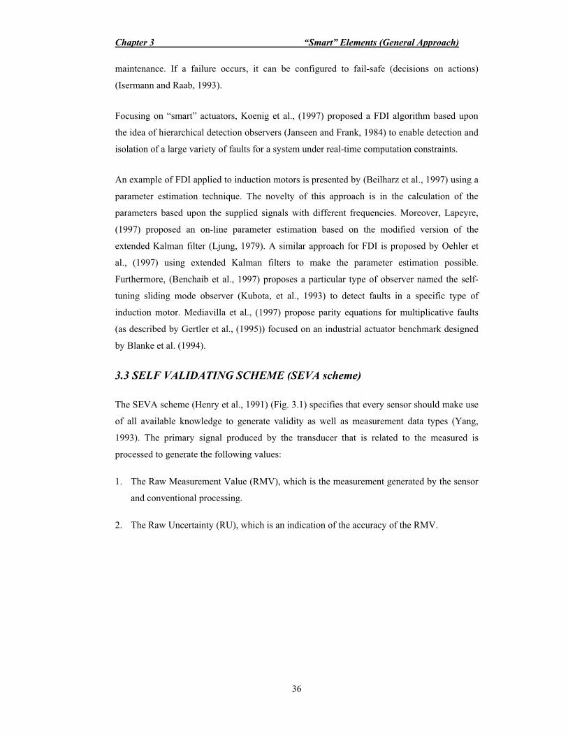
Chapter 3 “Smart” Elements (General Approach)
36
maintenance. If a failure occurs, it can be configured to fail-safe (decisions on actions)
(Isermann and Raab, 1993).
Focusing on “smart” actuators, Koenig et al., (1997) proposed a FDI algorithm based upon
the idea of hierarchical detection observers (Janseen and Frank, 1984) to enable detection and
isolation of a large variety of faults for a system under real-time computation constraints.
An example of FDI applied to induction motors is presented by (Beilharz et al., 1997) using a
parameter estimation technique. The novelty of this approach is in the calculation of the
parameters based upon the supplied signals with different frequencies. Moreover, Lapeyre,
(1997) proposed an on-line parameter estimation based on the modified version of the
extended Kalman filter (Ljung, 1979). A similar approach for FDI is proposed by Oehler et
al., (1997) using extended Kalman filters to make the parameter estimation possible.
Furthermore, (Benchaib et al., 1997) proposes a particular type of observer named the self-
tuning sliding mode observer (Kubota, et al., 1993) to detect faults in a specific type of
induction motor. Mediavilla et al., (1997) propose parity equations for multiplicative faults
(as described by Gertler et al., (1995)) focused on an industrial actuator benchmark designed
by Blanke et al. (1994).
3.3 SELF VALIDATING SCHEME (SEVA scheme)
The SEVA scheme (Henry et al., 1991) (Fig. 3.1) specifies that every sensor should make use
of all available knowledge to generate validity as well as measurement data types (Yang,
1993). The primary signal produced by the transducer that is related to the measured is
processed to generate the following values:
1. The Raw Measurement Value (RMV), which is the measurement generated by the sensor
and conventional processing.
2. The Raw Uncertainty (RU), which is an indication of the accuracy of the RMV.

Chapter 3 “Smart” Elements (General Approach)
37
ConventionalProcessing Diagnostics
Generate OutputData Types
Device-SpecificTests
RawData
RMVRU
DiagnosticState VMV
VUMV Status
DeviceStatus
RMV
DetailedDiagnostics
auxiliary signalother Information
Fig. 3.1 SEVA Implementation
Yang states (1993): In the SEVA scheme it is first necessary to identify all the sources of
errors and evaluate the uncertainty contributed by each of them. These components are
combined in conformity with the measurement model to give an on-line estimate of the
measurement uncertainty.
Process
m1 mi
eje1
(de1)2 (dej)
2
(dm1)2 � � � �� �
�
���
� 2
2
2j
j
ii de
dedmdm
� � � �� ��
���
� 2
22
0 ii
dmdmdfPd
� � � � � �22
0
2 ˆˆˆunknownPdPdPd ��
Fig. 3.2 SEVA approach to Uncertainty Analysis
Fig. 3.2 shows the approach adopted by SEVA in order to analyse the uncertainties of the
process on-line. There are several components involved in this procedure. First, there are m
different measured variables from the same process. Each of these has different error sources
ej which it is necessary to identify. Second, the evaluation of the square root of the second
moment of the distribution due to each error source is performed (dej)2. Third, the evaluation

Chapter 3 “Smart” Elements (General Approach)
38
of the second power equation which is a standard for the uncertainty evaluation (Yang, 1993)
is the sum of the errors and their impact on the measured variable
� � � �� ��
���
� 2
22
jj
ii de
dedm
dm (3.1)
Fourthly, the evaluation of the overall measured uncertainty over the process P0 is performed:
� � � �� ��
���
� 2
22ˆ
ii
o dmdmdfPd (3.2)
Finally, the estimation of the total uncertainty, � �2Pd , over the process P is calculated using
two main terms:
� The measured uncertainty � �2ˆoPd .
� The heuristic uncertainty determined by the experience of the designer � �2unknownPd .
The relation between the measured variables mi and errors ej is determined by the analysis of
the dynamics of the element and the impact of the error (eqn. 3.1). The result of the analysis
of the uncertainties (dmi)2 from the measured variables mi into the process P follows the same
strategy as eqn. 3.1 (see eqn. 3.2). Therefore, the mathematical relation between each
component of the sensor and the final output must be known in order to determine the effects
of the uncertainties in the final result.
Table 3.1 shows a comparison of conventional uncertainty analysis against the SEVA
approach (Yang, 1993).
Conventional Approach SEVA Approach Types of Uncertainty Differentiate between random
and systematic uncertainties Only one type of uncertainty
Propagation of Uncertainty Second-power equation invoked outside sensor
Applied within the sensor and considers all error sources
Reported Uncertainty Fixed value Values vary with measurement and operating condition (determined off-line)
Table 3.1 Comparison between SEVA and Classical Approaches
By considering all sources of information currently available, the sensor makes an internal
assessment of its own condition and performance to arrive at a diagnostic state. Based on this,

Chapter 3 “Smart” Elements (General Approach)
39
appropriate strategies are selected for generating a set of standard metrics for each
measurement:
1. The Validated Measurement Value (VMV).
2. The Validated Uncertainty (VU).
3. The Measurement Value Status (MV Status). This is assigned a value determined from
the current Diagnostic State. There are six possible values:
� Clear: The measurement has been calculated normally with no faults.
� Blurred: A fault has been detected and VMV is generated by compensating RMV.
� Dazzled: The RMV is virtually aberrant, nevertheless the fault is considered
temporary. The VMV is generated from past history.
� Blind: The measurement capability has been destroyed completely. The VMV is
generated from past history.
� Secure: The VMV is generated from redundant fault free sources. The confidence in
each measurement is nominal.
� Unvalidated: Validation is not taking place.
4. Device Status. This value indicates whether or not the instrument is in need of
maintenance. This value summarises the health of the sensor. There are six possible
values:
� Good: The sensor is operating normally.
� Testing: The sensor is performing a diagnostic test due to a loss of measurement
quality.
� Suspect: There is an aberration. This has not been diagnosed.
� Impaired: The sensor is suffering from a fault. This has a minor impact on
performance.
� Bad: The sensor is suffering from a fault. This has a major impact on performance.
� Critical: The sensor is in a dangerous condition. It requires immediate observation.

Chapter 3 “Smart” Elements (General Approach)
40
Clearly, a SEVA sensor is a much more useful source of information compared with a
conventional device. It supplies not only a validated version of the measurement, but also
provides vital information about the quality of the measurement to both the control and alarm
systems. Making use of internal signals (such as the measurement of the parameters of the
sensor), the sensor is more likely to detect and diagnose sensor faults and process aberrations
than conventional FDI schemes by the analysis of the uncertainties. The complex device
functions need not be visible outside the sensor. The SEVA scheme is based upon the
uncertainty measure of each component within the main sensor. The novelty of this approach
is the evaluation of the uncertainty on-line as a result of the uncertainty analysis on-line of the
whole SEVA sensor. This scheme does not use the classical fault diagnosis approach.
3.4 MODIFIED SEVA
3.4.1 Limitations of SEVA for Fault Detection and Isolation
Using uncertainty analysis it is possible to determine the effects of faults on local elements in
the “smart” unit. The analysis of FDI permits the identification of a fault in the monitored
element whereas the SEVA scheme simply measures the degradation of the “smart” element
rather than the diagnosis of the fault. The use of uncertainty information from different error
sources such as parameters and the design of a suitable parameter estimation technique (Fig.
3.3) can carry out the analysis for SEVA. However, the computational cost could be high and
the analysis must be specific to the dynamic characteristics of the particular “smart” unit.
As mentioned earlier, an alternative technique is parameter estimation by comparison of the
measurements available from the current model and parameter estimation on-line.
Information about the uncertainties of the measurements can be added to the parameter
estimation model in order to define the degradation of the “smart” element. Fig. 3.3 shows
this first approach.
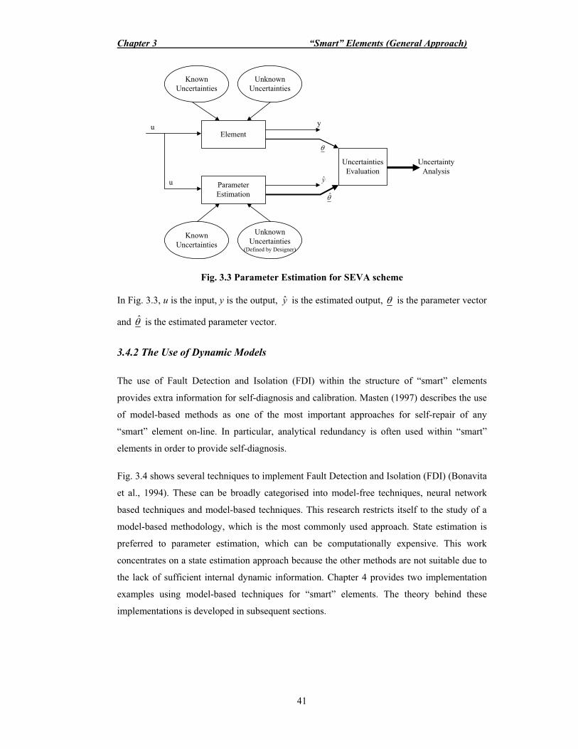
Chapter 3 “Smart” Elements (General Approach)
41
ParameterEstimation
KnownUncertainties
KnownUncertainties
UnknownUncertainties
UnknownUncertainties
(Defined by Designer)
u
u
y
y
�
�
UncertaintyAnalysis
UncertaintiesEvaluation
Element
Fig. 3.3 Parameter Estimation for SEVA scheme
In Fig. 3.3, u is the input, y is the output, y is the estimated output, � is the parameter vector
and � is the estimated parameter vector.
3.4.2 The Use of Dynamic Models
The use of Fault Detection and Isolation (FDI) within the structure of “smart” elements
provides extra information for self-diagnosis and calibration. Masten (1997) describes the use
of model-based methods as one of the most important approaches for self-repair of any
“smart” element on-line. In particular, analytical redundancy is often used within “smart”
elements in order to provide self-diagnosis.
Fig. 3.4 shows several techniques to implement Fault Detection and Isolation (FDI) (Bonavita
et al., 1994). These can be broadly categorised into model-free techniques, neural network
based techniques and model-based techniques. This research restricts itself to the study of a
model-based methodology, which is the most commonly used approach. State estimation is
preferred to parameter estimation, which can be computationally expensive. This work
concentrates on a state estimation approach because the other methods are not suitable due to
the lack of sufficient internal dynamic information. Chapter 4 provides two implementation
examples using model-based techniques for “smart” elements. The theory behind these
implementations is developed in subsequent sections.

Chapter 3 “Smart” Elements (General Approach)
42
Fault Detection andIsolation Methods
Model-Free NeuralNetworks Model-Based
KnowledgeRedundancy
AnalyticalRedundancy
ParameterEstimation
StateEstimation
Fig. 3.4 Classification of Analytical Redundancy
The dotted lines in Fig. 3.4 show the procedure followed in this thesis.
The use of state-space models enables the introduction of observers to estimate the “actual”
states of the element. There is a detailed explanation of the observer implemented in Section
3.4.3.
As described in Chapter 2, a fault is a physical defect or imperfection that occurs within some
hardware or software component. However, this definition can be rewritten based upon the
behaviour of the system dynamics. Therefore, a fault may be defined as an unpermitted
deviation of at least one characteristic property of a variable from an acceptable behaviour
(Isermann, 1997). Thus, the fault is indicated by a state that may lead to a malfunction or
failure of the system.
Fault detection by analytic and heuristic symptom generation and fault diagnosis are the main
uses of analytical redundancy (Isermann, 1997). To do this, data processing based on
measured process variables, has to be performed to generate values by:
� limit value checking of direct, measurable signals,
� signal analysis of directly measurable signals by the use of signal models,
� process analysis by using mathematical process models together with parameter
estimation, state estimation and parity equation methods. The characteristic values are
parameters, state variables and residuals.
These features are compared against normal features of the fault-free process. The resulting
changes in the directly measured signals, signal models or process models are considered to
be analytic symptoms.
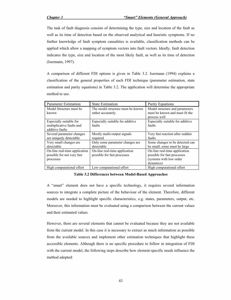
Chapter 3 “Smart” Elements (General Approach)
43
The task of fault diagnosis consists of determining the type, size and location of the fault as
well as its time of detection based on the observed analytical and heuristic symptoms. If no
further knowledge of fault symptom causalities is available, classification methods can be
applied which allow a mapping of symptom vectors into fault vectors. Ideally, fault detection
indicates the type, size and location of the most likely fault, as well as its time of detection
(Isermann, 1997).
A comparison of different FDI options is given in Table 3.2. Isermann (1994) explains a
classification of the general properties of each FDI technique (parameter estimation, state
estimation and parity equations) in Table 3.2. The application will determine the appropriate
method to use.
Parameter Estimation State Estimation Parity Equations Model Structure must be known
The model structure must be known rather accurately
Model structure and parameters must be known and must fit the process well
Especially suitable for multiplicative faults and additive faults
Especially suitable for additive faults
Especially suitable for additive faults
Several parameter changes are uniquely detectable
Mostly multi-output signals required
Very fast reaction after sudden faults
Very small changes are detectable
Only some parameter changes are detectable
Some changes to be detected can be small, some must be large
On-line real-time application possible for not very fast processes
On-line real-time application possible for fast processes
On-line real-time application possible for fast processes (systems with low order dynamics)
High computational effort Low computational effort High computational effort
Table 3.2 Differences between Model-Based Approaches
A “smart” element does not have a specific technology, it requires several information
sources to integrate a complete picture of the behaviour of the element. Therefore, different
models are needed to highlight specific characteristics, e.g. states, parameters, output, etc.
Moreover, this information must be evaluated using a comparison between the current values
and their estimated values.
However, there are several elements that cannot be evaluated because they are not available
from the current model. In this case it is necessary to extract as much information as possible
from the available sources and implement other estimation techniques that highlight these
accessible elements. Although there is no specific procedure to follow in integration of FDI
with the current model, the following steps describe how element-specific needs influence the
method adopted:

Chapter 3 “Smart” Elements (General Approach)
44
� Observe the model of the element in fault-free conditions and determine the nature of the
non-linearities and those parameters (states, physical parameters and outputs) that are
available for comparison in FDI.
� Propose the most suitable FDI technique for the model. This technique must be stable and
represent the non-linearities. It must also highlight those parameters that are analysed
from the element (for instance, pressure). In particular, if the technique used is an
estimation procedure (parameter estimation, parity equations, state estimation), it should
be focused and highlight those elements that are available from the model. In the case of
the proposed technique, the estimating procedure is that of state estimation. The main
problem is to determine all the knowledge sources that are required considering the
possible fault scenarios.
� If the FDI technique is an estimation technique (as is used in this research), the next stage
is the comparison (calculation of the symptom vector) between the current values from
the element (considering parameters and states) and their estimates. This comparison
should emphasise those differences arising from the possible presence of a fault. The
presence of non-linearities or unmodelled conditions must have a limited impact on the
result of the residual vector.
� The evaluation of the residual vector to determine the presence of a fault and the impact
that it has on the element is carried out in a non-linear manner. There are several
techniques that could be used for this evaluation, for example, fuzzy logic. Regardless of
the technique used, the result of this residual evaluation must be stable even in
catastrophic conditions. Therefore, the use of categorisation counters (or fault tolerance
integrators) during a time window in order to eliminate any spike or transitory fault
provides the most suitable solution to this typical problem. Hence, based upon the scheme
explained in Section 3.3, there are three main goals to be achieved by the modification of
SEVA (see Section 3.4.5.1):
1. The Confidence Value represents a measure of the degradation of the system due
to the presence of a fault. This measure is based upon an analysis of the output
and the element dynamics. The range of the Confidence Value varies between 0
and 1, where 0 represents a catastrophic situation and 1 a fault free scenario.
2. The Device Evaluation represents a measure of the degradation of the element
dynamics due to the presence of a fault. This measure is primarily based upon an
analysis of the system dynamics. The signal is assigned integer values between 0
and 5, where each value has a specific meaning (see Table 3.3 in Section 3.4.5.1).
Chapter 3 “Smart” Elements (General Approach)
45
3. The Measurement Evaluation represents a measure of the degradation of the
output signal due to the presence of fault. This measure is primarily based upon
an analysis of the output signal. The signal is assigned integer values between 0
and 5, where each value has a specific meaning (see Table 3.4 in Section 3.4.5.1).
3.4.2.1 Parameter Estimation
In many practical cases, the process parameters are not known at all, or are not known well
enough. In this case they can be determined using parameter estimation methods by
measuring input and output signals if the basic structure of the model is known (Gertler,
1998). The process model is considered non-linear g(u,t) and is expressed as in eqn. (3.3.a). In
terms of parameter estimation, this is written in the vector form, eqn. (3.3.b), with the
parameter and discrete-time data vectors. For parameter estimation the equation error e(t) is
introduced by eqn. (3.4):
),()( tugty � (3.3.a)
�� )()( tty T� (3.3.b)
�� )()()( ttyte T�� (3.4)
where ]......[ 11 mnT bbaa�� (3.5)
and )](),...,(;)(),...,([ nTtutunTtytyT ������ (3.6)
where � (eqn. 3.5) is the vector related to the parameters ai and bi of the non-linear function
g(u,t). y(t) represents the output and e represents the error between the current system and its
estimate.
Generally, the process parameters � depend on physical process coefficients p such as
inductance or capacitance:
� � f p( ) (3.7)
via non-linear algebraic equations. This physical dependency holds if and only if the inversion
of this relationship (eqn. 3.7) is possible in eqn. (3.8)
p f� �1( )� (3.8)
Chapter 3 “Smart” Elements (General Approach)
46
Changes in p (�p) are directly related to the faults and can be calculated in any condition
(Isermann, 1994). Therefore, knowledge of �p, as the modification of the process coefficients
due to the presence of a fault, facilitates fault diagnosis. Parameter estimation can also be
applied to non-linear static process models (Isermann, 1994). This technique performs well in
ideal conditions, say, for multiplicative faults and for systems with a low-frequency response
compared with the state estimation approach. Also, it is necessary to know the mathematical
relationship between the parameters � and p in order to detect any deviation between the
current process and its estimate. This last assumption is not always possible and depends on
the dynamics of the “smart” unit.
3.4.2.2 State Estimation and Observers
A linear process can be described in state-space form as
)()()()()()()(
tDutxCtytdEtuBtxAtx
������ (3.9)
Here, input signals u(t) and output signals y(t) are assumed to be vectors in order to be
suitable for multivariable systems. Matrices A, B, D, E and C represent the parameters of the
model and x represents the states of the model. d(t) is the disturbance vector. Assuming that
the structure and all process parameters A, B, C, are known and D is zero, a state observer can
be used to reconstruct the unmeasurable state variables based on the measured inputs and
outputs:
)(ˆ)()()()(ˆˆ
txCtyteteHtuBxAx
������
(3.10)
where �x is the estimated state vector and H is the matrix which permits the estimation from
the observer that is proposed by the designer (Isermann, 1994). The error, e, is compared with
the current output, y. For the state estimation error, it follows, eqn. (3.11), that
xHCAx
xxx~][~
ˆ~
��
���
��� (3.11)
where x~ is the state estimation error vector that asymptotically converges to zero. Section
3.4.3 presents a detailed review and comparison of different approaches for observers.

Chapter 3 “Smart” Elements (General Approach)
47
3.4.2.3 Parity Equations
A straightforward model-based method of fault detection is to take a fixed estimated model
Gm and to run it in parallel with the process Gp to obtain an output error, r(s),
)()]()([)( susGsGsr mp �� (3.12)
To generate specific properties, the residuals can be filtered:
r s G s r sf f( ) ( ) ( )� (3.13)
This method of estimation is restricted to low-frequency systems. The plant model must be
observable in order to permit the use of parity equations (Isermann, 1994). Parity equations
can be transformed to a parameter estimation technique by the use of a filter with r(s)
(Gertler, 1991). The main disadvantage of parity equations is the computational effort
involved and the fact that the knowledge of the fault and its effect on the parameters (Gertler,
1998) must be known.
3.4.3 Non-Linear Observers
In this section, three non-linear observers are considered for the problem of non-linear
estimation. Fig. 3.5 shows the integration of the possible observer into the topology of the
“smart” element. The output of this technique is the estimated output, y , and estimated state
vector, x .
Element
Observer
Disturbances Disturbances
u y+
+ +
+
xy
Fig. 3.5 Integration of an Observer Technique into the “Smart” Element
In the first approach Chen et al., (1995) describe a class of systems in which the system
uncertainty can be summarised as an additive unknown disturbance term d(t), as follows:
)()()()()()(
txCtytdEtuBtxAtx
�����
(3.14.a)

Chapter 3 “Smart” Elements (General Approach)
48
and )(ˆ)()(~ txtxtx �� (3.14.b)
where x(t) is the state vector, y(t) is the output vector, u(t) is the known input vector and d(t)
is the unknown input vector. A, B, C and E are known matrices with appropriate dimensions.
An unknown input observer for the system described in eqn. (3.14.a) can be defined if its state
estimation error vector )(~ tx approaches zero asymptotically regardless of the input
conditions (eqn. 3.14.b). The structure for this full-order observer is given by:
)()()(ˆ)()()()(
tyHtztx
tyKtuTBtzFtz
��
���� (3.15)
where )(ˆ tx is the estimated vector, z is the state of this full-order observer and F, T, K, H are
matrices to be designed for achieving unknown input decoupling. H and K are chosen such
that )(~ tx tends to zero. F and T are defined from A, B, H and K matrices. However, the
design of asymptotically stable observers is a difficult task in the non-linear case, even when
the nonlinearities are fully known (Adjallah et al., 1994). Therefore another approach was
sought.
In this second approach Frank (1994a) proposes a methodology for the creation of non-linear
observers. In this approach the model of the system is given by the non-linear state equations:
2
1),(
),(
fuxcy
fuxfx
��
��� (3.16)
where f1 and f2 denote the possible faults, modelled in the form of external unknown input
signals. The idea of a linear unknown input fault detection observer can be readily extended to
a certain class of non-linear systems described by:
2222
1111),(
fKdExCy
fKdEuyBxAx
���
����� (3.17)
where K1 and K2 are known matrices, the signals d1 and d2 represent unknown inputs, the
terms f1 and f2 are additive faults and the term B represents the non-linearity of the plant. This
term is defined in terms of y and u. In fact, external disturbances are considered within the
matrix B which are from y and u. These variables determine the behaviour of the non-
linearity. Since the non-linear term B(y,u) depends only on y and u it is possible to

Chapter 3 “Smart” Elements (General Approach)
49
compensate completely for the non-linearity by the use of estimation from an observer of the
form:
yLxLe
yGuyJxFx
21 ˆ),(ˆˆ
��
���� (3.18)
where F, G, J, L1 and L2 matrices are proposed based upon the result of eqn. (3.19). The term
x corresponds to the state estimation and e represents the error vector. The conditions which
need to be met by the observer matrices from the unknown inputs d1 and d2 and sensitivity to
the faults f1 and f2 can be stated as follows:
)()(0
00
0
),(),(,
11
21
22
2
1
KrankTKrankCLTL
ELGETE
uyTBuyJFstableGCFTTA
���
���
���
(3.19)
A characteristic of this type of system is that the measurement is only corrupted by faults and
not by unknown inputs (Frank, 1990). The definition of T becomes crucial for this model and
it is restricted by B(y,u). B(y,u) must be the only non-linear matrix for the observer otherwise
T becomes unstable. Eqn. 3.19 shows that F cannot suffer any variation, therefore, G, L1 and
L2 must be defined in terms of B and T. For most of the cases of non-linear elements (in
particular sensors), it is not possible to establish the non-variation of F. Hence, T cannot be
properly defined in order to reach a stable observer.
A third approach is now considered, based upon adaptive observers. The use of adaptive
observers is becoming an increasingly attractive solution for a great variety of non-linear
systems. For instance, Schreier et al. (1997) design an observer based upon:
xCytutxdBuxAx
���� ))(),((�
(3.20)
where A, B and C are constant. x represents the state vector, y the output, u the input and d
the non-linear function. In this approach it is necessary to supply an upper bound for the non-
Chapter 3 “Smart” Elements (General Approach)
50
linearity that guarantees the stability of the state estimation. This bound is given by two
hypotheses (H1) and (H2):
(H1) d(.) must satisfy the Lipschitz condition (Schreier et al., 1997) with constant k:
xxkuxduxd ˆ),ˆ(),( ���
(H2) The pair (A,C) are observable
where x and x are the estimated state and the actual state vectors, respectively.
The observer estimates the states under the two hypotheses H1 and H2. The stability of this
observer is evaluated by an iterative process (Schreier et al., 1997) under the assumptions H1
and H2, an observer of the following form can be defined:
xCyyyCSuxdBuxAx T
ˆˆ)ˆ()(),(ˆˆ 1
������ ���
(3.21)
where S(�) is the solution of the Lyapunov equation:
A S S A C C ST T( ) ( ) ( )� � � �� � � � 0 (3.22)
with � chosen to be a positive parameter under the constraint that the matrix S is positive
definite. The term ),ˆ( uxd represents the nonlinearities of the model (eqn. 3.20). A drawback
of this observer is the definition of � which depends on the definition of the condition H1.
This variable must be optimal with respect to the Lipschitz condition. This cannot be achieved
on-line which is required for the performance of the “smart” element.
In order to evaluate these three approaches (observers) it is important to consider non-linear
elements, in particular, the pressure sensor and fuel valve actuator explained in Chapter 4.
The expected response for these approaches was a non-modification of the residual vector
with respect to fault free scenarios. However, there were certain variations due to the
imprecision of the system modelling dependent on the implementation of the three observer
approaches.
In the first approach T, K and H matrices (eqn. 3.15) have a relation based upon the estimation
error. There is no guarantee of achieving stability at every operating point within this
estimation, because of the predefinition of H. It is, however, possible to apply recursive
criteria to achieve stability, although it is not completely accurate with respect to the non-

Chapter 3 “Smart” Elements (General Approach)
51
linear case. For the second case, the stability equation requirements (eqn. 3.19) are not
obtainable due to the variability of T. Alternatively, Schreier’s approach has a stability
criterion based upon a Lyapunov analysis (eqn. 3.22). This process permits stability to be
achieved through the solution of the inherent recursive criteria based upon the definition of
the boundary k. However, it is necessary to define the correct value related to the optimal � in
order to obtain a stable observer. This last approach cannot be reached on-line.
An alternative procedure is the Kalman filter. This well known observer offers the advantage
of adaptation on-line for different non-linear scenarios. The algorithm used here is based upon
that proposed in the Control Systems Toolbox Matlab manual (Control Systems Toolbox,
1990). This implementation has the advantage of a fast response with respect to transitions
from one operating point to another. Appendix B.1 shows a general implementation.
3.4.4 Residual Generation
The next step is to propose a particular evaluation to generate the residual vector. The most
straightforward and simple evaluation is the difference between the current values and their
estimates:
Residual Vector => r =��
���
���
xxyyˆˆ (3.23)
This strategy gives the possibility of evaluating the amplitude variation. The first variation
(output variation) shows the effects of the faults, whilst the latter shows the effects but in
terms of the difference in states. This vector identifies which output/state has been affected
and by how much.
In addition to this evaluation there are other techniques that can be useful for the extraction of
information, for instance, normalisation of the vector gives a smooth change of the result
avoiding spikes. There are many other non-linear techniques that can be used to emphasise
specific fault behaviour, however, the most useful and efficient technique that can be used in
a wide range of scenarios is that proposed in eqn. 3.23.
This vector is passed to an evaluation procedure that is made up of different fuzzy systems
(Fig. 3.6). The main task is to evaluate the scenario and translate this information into
different categories expressed by Confidence Value, Device Evaluation and Measurement
Evaluation. This procedure must perform correctly in different fault-free scenarios and it has
to be insensitive to unmodelled non-linearities. In fault conditions it highlights the effects of
the different fault scenarios.
Chapter 3 “Smart” Elements (General Approach)
52
Having defined the residuals, the next step is to establish the methodology for their
evaluation. Different strategies can be proposed such as structured or directional residuals
(Gertler, 1998). The use of either of these two techniques has the advantage of identifying a
fault based upon the relationship between the residuals and the appearance of a fault. In
particular, directional residuals present a better approach in terms of a graphical
representation for the identification of a fault.
Another choice is based upon the evaluation of the residuals by the use of fuzzy logic in order
to identify the degradation of trust in the element when a fault is present. This has been
explored in this thesis using the modified SEVA scheme.
3.4.5 Implementation of Modified SEVA scheme
Use of the SEVA scheme provides a communication standard giving to the health of the
“smart” sensor. It was necessary to modify the original SEVA scheme for the problem
domain studied here. This modification is due to the fact that the analysed elements do not
have certain sources of information required in order to generate the SEVA scheme. The
scope of modified SEVA scheme is to measure the degradation in the dynamics of the
element (sensor/actuator) from various dynamic information sources (parameters, states and
outputs). This technique is based upon the evaluation of the element using analytical
redundancy strategies. In contrast, the SEVA scheme evaluates the element from the analysis
of the uncertainties (Fig. 3.2). The measures used do not relate the dynamic of the sensor to
the uncertainties. They concentrate on the degradation of the final output with respect to the
uncertainty.
The modified SEVA scheme is based upon the necessity for a communication standard for a
self-diagnostic procedure. In this modified scheme, this is the output of a fuzzy evaluation of
the residual vector. Fig. 3.6 shows this general procedure. This consists of two main blocks,
the residual evaluation procedure and the fuzzy evaluation procedure. The first block
calculates the difference between the current output and states and their estimated values. The
second block evaluates the result of the previous calculation to produce the Modified SEVA
scheme based upon three signals:
1. Confidence Value
2. Device Evaluation
3. Measurement Evaluation
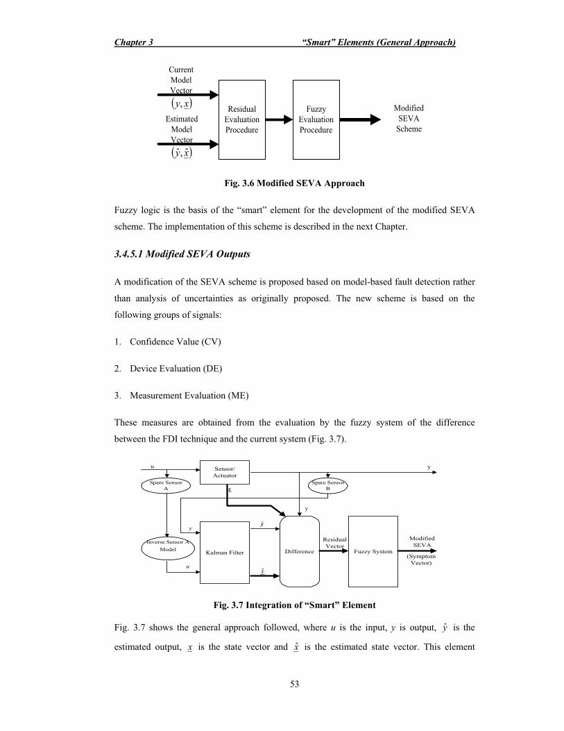
Chapter 3 “Smart” Elements (General Approach)
53
CurrentModelVector
EstimatedModelVector
ModifiedSEVA
Scheme
� �xy,
� �xy ˆ,ˆ
ResidualEvaluationProcedure
FuzzyEvaluationProcedure
Fig. 3.6 Modified SEVA Approach
Fuzzy logic is the basis of the “smart” element for the development of the modified SEVA
scheme. The implementation of this scheme is described in the next Chapter.
3.4.5.1 Modified SEVA Outputs
A modification of the SEVA scheme is proposed based on model-based fault detection rather
than analysis of uncertainties as originally proposed. The new scheme is based on the
following groups of signals:
1. Confidence Value (CV)
2. Device Evaluation (DE)
3. Measurement Evaluation (ME)
These measures are obtained from the evaluation by the fuzzy system of the difference
between the FDI technique and the current system (Fig. 3.7).
Sensor/Actuator
Kalman Filter Difference Fuzzy System
u y
ModifiedSEVA
y
�y
ResidualVector
(SymptomVector)
Spare SensorA x
x
y
u
Spare SensorB
Inverse Sensor AModel
Fig. 3.7 Integration of “Smart” Element
Fig. 3.7 shows the general approach followed, where u is the input, y is output, y is the
estimated output, x is the state vector and x is the estimated state vector. This element

Chapter 3 “Smart” Elements (General Approach)
54
considers a main component (sensor/actuator). The use of extra sensors provides the ability of
access extra information such as the input (in the case of a “smart” sensor) or the output (in
the case of a “smart” actuator). The use of inverse sensor model within the “smart” element
provides a much closer reading of the current measure of the spare sensor. This information is
use by the analytical redundancy technique in order to evaluate the element.
The output vector of this element, different characteristics were chosen. For the Confidence
Value a range from 0 to 1 was chosen. For the Device and Measurement Evaluation signals an
integer range from 0 to 5 was chosen. The Confidence Value is a representation of the
accuracy of the current value produced by the element. Its evaluation utilises the residual
between y, the states and the estimated values ( y , x ). The Device Evaluation is produced
from the residual between x and x . The Measurement Evaluation uses the current output y
and the estimate �y . From this explanation a list of the inputs for each signal is given:
� Confidence Value
� The residual of the output and the residual of the states are the inputs for this signal.
Every residual has the same impact on the Confidence Value.
� Device Evaluation
� The residuals of the states (parameters) are the most important evaluation elements
for DE.
� The residual of the output is considered.
� Measurement Evaluation
� The residual of the output is the most important evaluation element for ME.
� The residuals of the states are considered.
CV, ME and DE are obtained from three fuzzy systems. The result of CV is given between 0
and 1 where 0 is a catastrophic condition and 1 is a fault-free scenario. Intermediate values
show the degradation of the element from one point to another (Fig. 3.8).

Chapter 3 “Smart” Elements (General Approach)
55
Time
Confidence Value
1
0
0.5
Degradatio
n
Low Confidence
High Confidence
Fig. 3.8 Confidence Value Interpretation
Measurement Evaluation and Device Evaluation are defined by labels from 0 to 5. The
information generated by both signals is converted to a corresponding label (Fig. 3.9).
Time
MeasurementEvaluation
secure
catastrophicblind
impropersuspicious
clear(5)
(4)
(3)
(2)
(1)(0)
Fig. 3.9.a Measurement Evaluation Labelling
Device Evaluation
Time
good
criticalbad
impropersuspicious
inconsistent(5)
(4)
(3)
(2)
(1)(0)
Fig. 3.9.b Device Evaluation Labelling
Measurement evaluation (ME) labelling (Fig. 3.9.a) differs from the labelling of the MV
status in the original SEVA scheme. These differences appear when the element recognises
the presence of a fault. In the case of the original SEVA scheme, the element uses past
information in order to generate a valid output in the presence of a fault (labels: Blurred,