Simulation and system identification of helicopter ... · regression in the domain of simulation...

ABSTRACTThis paper provides an overview of techniques developed for the application of support vector regression in the domain of simulation and system identification of helicopter dynamics. A generic high fidelity FLIGHTLAB helicopter model is used to train and validate a number of pitch response SVR models. These models are then trained using flight data from a Sikorsky Seahawk helicopter. The SVR simulation results show significant promise in the ability to represent aspects of a helicopter’s dynamics at a high fidelity. To achieve this, it is important to provide the SVR kernel with knowledge of past inputs that encompass the delay characteristics of the helicopter dynamic system. In this case, the use of nonlinear auto regressive eXogenous input network architecture achieves this goal. Good performance was achieved using input data that encompassed between 300 to 500ms worth of historic response.

NOMENCLATUREb hyperplane constantC regularisation coefficienti, j individual data points (i, j = 1:N)k SVM kernel functionN number of training pointsw hyperplane normal vectorx input vector

The AeronAuTicAl JournAl December 2015 Volume 119 no 1222 1541

Paper No. 4354. Manuscript received 7 February 2015, revised version received 7 May 2015, accepted 24 July 2015.This is an adapted version of a paper first presented at The 40th European Rotorcraft Forum

hosted by the Royal Aeronautical Society in Southampton, UK, September 2014.

Simulation and system identification of helicopter dynamics using support vector regressionS. MansoDefence Science & Technology OrganisationFishermens BendAustralia

1542 The AeronAuTicAl JournAl December 2015

X input space, where input vector is definedXB longitudinal cyclic control inputy output valueZ feature spaceα, α Lagrangian multipliersε insensitive factorζ, ξ slack variablesΦ regression functionφ non-linear mapping

ABBREVIATIONSADF Australian Defence ForceAMAFTU Aircraft Maintenance and Flight Trials UnitART Advanced Rotorcraft TechnologyDSTO Defence Science & Technology OrganisationERM empirical risk minimisationHMI human machine interfaceMISO multiple input single outputMQL mean quadratic lossNARX nonlinear auto regressive exogenousQP quadratic programmingRBF radial basis functionSRM structural risk minimisationSV support vectorSVM support vector machineSVR support vector regressionTDL tapped delay lines

1.0 INTRODUCTIONThis paper provides an overview of techniques developed for the application of support vector regression (SVR) in the domain of simulation and system identification of helicopter dynamics. SVR is a machine-learning technique that provides a ‘black box’ approach that may enable a more simplistic method for simulation whilst retaining acceptable levels of accuracy. SVR is the regression form of the more widely used support vector machine (SVM) classification method. In this paper, the term SVM will refer to both the classification and regression methods, whereas SVR will specifically be used for the regression form.

The basis of the following work originally stemmed from the growing levels of complexity required from simulators to appropriately represent the rotary wing platforms in use by the Australian Defence Force (ADF). The ADF is currently acquiring and transitioning into service, multiple helicopter platforms including the Eurocopter ARH Tiger, NHIndustries MRH-90, Sikorsky MH-60R, and Boeing CH-47F, all of which require simulation support. The Australian Defence Science & Technology Organisation (DSTO) provides some of this support. DSTO uses flight dynamic simulators to perform human machine interface (HMI) studies, and to assist in accident investigation.

mAnso simulATion AnD sysTem iDenTificATion of helicopTer DynAmics using ... 1543

At present, the traditional technique for the dynamic modelling of helicopters and their systems involves the collection of flight data and aircraft specifications from which physics based theoretical equations are generated and validated. It is a time consuming process that requires the availability of a significant amount of data. The data required is often proprietary or commercial-in-confidence, leading to a lack of availability, which can result in less than optimal simulations(1).

Another modelling approach involves the system identification of helicopter dynamics using frequency analysis techniques(2). This is a parameter estimation method in which measured aircraft responses are essentially inverted to extract a subset of the system model. This modelling approach requires flight data for aircraft response to a control input frequency sweep. Such flight data can be difficult to obtain from non-flight-test aircraft due to the inherent risk of airframe structural stress when undertaking frequency response manoeuvres.

The implementation of a black box approach using machine-learning techniques may provide an option for a more simplistic method of simulation. A black box model can be defined as a machine with known or specified performance characteristics but whose constituents and means of operation are not necessarily known or specified by the user. For a given set of inputs, an expected set of outputs can be generated without explicitly knowing the relationship between input and output. A black box simulation would ideally only require flight data that is readily available to the operator of the helicopter platform, such as aircraft attitude response to pilot cyclic control inputs. Data could be captured using either existing aircraft systems, or via retrofitted instrumentation.

Machine learning, using methods such as neural networks and more recently SVMs, are popular for the implementation of black box modelling. The choice of using SVR for this investigation rather than other techniques based on neural networks is due to the increased exposure and promised advantages of SVMs, including being easier to train and having more robust learning.

2.0 SUPPORT VECTOR MACHINESSVMs arose from the area of statistical learning theory(3) and were originally proposed by V.N. Vapnik(4) in the early 1990s for the application of pattern classification. Since his seminal work, SVMs have been applied to a multitude of applications and undergone various transformations. Although the primary use of SVMs remains predominantly in the domain of classification, of particular interest is their use for regression in the form of SVR.

2.1 A comparison with other machine learning techniques

Since their inception, SVMs have been quite successful in solving real life problems and increasing the interest in statistical learning theory. Applications vary from face recognition(5) and text catego-risation(6) to predicting stock market indices(7) and modelling aerodynamic data(8).

Scholkopf et al(9) provided one of the original comparisons for classification between an SVM with Gaussian kernel, a support vector (SV) method hybrid with back-propagation, and a classical radial basis function (RBF) machine. The results show that the SVM reached highest accuracy in the application of handwritten digits recognition. Another early SVR comparison was conducted by Mukherjee et al(10). Various approximation techniques including neural networks and RBFs were applied to a chaotic time series. The SVM algorithm showed excellent performance here as well, outperforming other functions in most cases.

SVMs have performed favourably when compared to neural networks. One of the more relevant comparisons for this investigation is that of Fan et al(8) who compare the generalisation ability of SVMs and neural networks in the field of modelling aerodynamic data.


The key performance differences between SVMs and neural networks relate to the minimisation principles(11) on which they are based. SVMs are founded on structural risk minimisation (SRM) that minimises an upper bound of the generalisation error, whereas neural networks are based on empirical risk minimisation (ERM) that minimises the error on the training data. ERM can lead to local minima and over-fitting issues that need to be addressed by elaborate learning techniques. In contrast SRM generates a unique solution. This makes the application of SVMs in the real world a much easier prospect by removing the complexity associated with neural network training for good general performance.

2.2 Support vector regression

A brief overview of SVR theory is presented below. A more thorough derivation is available from Vapnik’s original work(4,11), as well as tutorials, examples and overviews available in the references(3,12-16).

Conceptually, SVM inputs are mapped to a higher dimensional, so-called feature space in which a decision surface lies. The support vectors themselves exist in the feature space of the SVM process and dictate the geometry of the decision surface. It is this decision surface that classifies each of the inputs in relation to the corresponding output, and it is the ability of the system to correctly classify previously unseen data, otherwise known as its ability to generalise, that dictates its usefulness. SVR differs from classification by approximating a function for the continuous output rather than that of a discrete response.

Given a set of N training points, where each example consists of an input vector, xi, and a label, yi, such that both are real:

. . . (1)

. . . (2)

The object is to find a regression function Ф(x) = y that can approximate any new examples with the same underlying probability distribution P(x, y).

To allow for nonlinear regression functions, the training points are mapped from the current input space X to a much higher dimensional feature space Z using a nonlinear mapping φ. The regression function Φ is defined to have at most ε deviation from the obtained targets yi for all the training data, where the constant ε is chosen by the user. In other words, all the training points must lie within ε > 0 of the following linear hyperplane in feature space:

. . . (3)

where w is the normal vector of the hyperplane, and the constant b is the bias.To deal with noisy data, slack-variables ζi and ξi are introduced to penalise points outside the

ε region. This corresponds to dealing with an ε-insensitive loss function defined by:

. . . (4)

The SVR solution can then be found by solving the primal quadratic programming problem (QP):

xi R⊆

y Ri ⊆

ˆ w b x x

ε

0 if otherwise


, subject to

. . . (5)

Conceptually, the first term achieves maximal margin for the hyperplane such that there is maximum distance between each of the points. The second term penalises the presence of any points outside the ε region. The constant C defines the trade-off between the two terms. The problem above represents a convex function with a unique minimum constrained to lie within a cube, although this solution occurs in the higher dimensional feature space due to the vector w.

Another formulation known as the dual QP problem is defined to constrain the solution to the input space, which is much simpler to compute. Suppose that the kernel k(xi, xj) is chosen such that the dot product in the feature space is equivalent to the kernel function in input space:

. . . (6)

Using Lagrangian multipliers αi and αi* with the kernel definition above, the dual formulation is

defined:

. . . (7)

subject to , and

Conceptually, the optimisation problem above corresponds to finding the flattest function in the feature space. Solving for αi and αi

*, the regression function for Φ is given by:

. . . (8)

2.3 Kernel functions

The constraint on the choice of kernel function in the SVM is to enable operations to be performed k(in the input space rather than the potentially high dimensional feature space. Specifically, the kernel k(xi, xj) chosen must satisfy the property such that the dot product in the feature space is equivalent to the kernel function in input space (Equation (6)). This provides a way of addressing the curse of dimensionality(17) which states that the difficulty of an estimation problem increases drastically with the dimension of the feature space.

Smola and Scholkopf(3) describe the theorems and relevant corollaries used to characterise such kernels. Several well-known functions that can be used as kernels are provided in Table 1. Other possible kernel types include Splines, closed form B Splines, additive summing of kernels and Tensor products. For the results presented herein, a linear kernel is used for its computational performance and simplicity.

min , ,*

w b i ii

N

w C 12

2

1

y w bw b yi i i

i i i

i i

xx *

*, 0

k i j i jx x x x,

max,* *

,

* *

1

2 1i i j j i j

i j

N

i i i i i

k

y

x x

i

N

i

N

11

i ii

N

*

100 i i C, *

*

1

ˆ ,N

i i ii

k b

x x x


3.0 MODELLING OF HELICOPTER FLIGHT DYNAMICSTo provide a complete mathematical simulation of a helicopter’s flight dynamics, one needs to represent the aerodynamic, structural and internal dynamic effects that once combined are influ-enced by the pilot controls and by external atmospheric disturbances(18). Helicopter behaviour is dominated by the rotor system, but limited by local effects that grow in influence at the limits of the flight envelope. These include, but are not limited to, blade stall, power limits, and control limits.

The method of modelling or extracting helicopter system dynamics or characteristics from flight test data is known as system identification. Machine learning techniques are a form of system identification when applied in this context.

There is little available in the literature on the use of SVMs for the system identification of a helicopter. Of most relevance is the recent work done by Bhandari et al(19) where an RBF kernel is investigated for the function estimation of a small scale helicopter. A few non-coupled models are developed to predict the longitudinal, lateral and tail rotor control inputs needed to achieve a desired flight trajectory, i.e. the inverse of a flight model. Flight data was initially post-processed through a Butterworth filter to reduce noise. Three data sets of 120Hz resolution were constructed for training, validation and test purposes. These data sets relate control input directly to the appro-priate angular rate of the aircraft. The initial SVR results look promising, although the extent of how well the model generalises is unclear.

Bhandari also developed a SVR model to predict pitch rate directly from longitudinal cyclic control, similar to the aims of this investigation. The testing and validation mean square errors are much higher than for the inverse problem above, yet the results show the correct trends. It is again unclear how well the model generalises or how the SVM was trained. It appears that input history was not implemented into their SVM model, likely resulting in the phase shifting of their results, and hence not suitable for dynamic modelling.

Table 1List of commonly used SVM kernels

Kernel Function Comments

Polynomial Becomes a linear kernel when d = 1

Radial basis Commonly referred to as the Gaussian function(Gaussian)

Radial basis Commonly referred to as the radial (Exponential) basis function (RBF)

Multi layer This is representative of the neural network equivalentperceptron

Fourier Series Defined on the interval

x xi j

d 1

exp

x xi j

2

22

exp

x xi j

2 2

Tanh i j x x Sin

Sin

N i j

i j

12

12

x x

x x

2 2

,


More progress with machine learning techniques is evident with the use of neural networks for helicopter system identification, particularly with the work of Mudigere, Kumar et al(20,21). The predicted response of various models to control inputs have been satisfactory, though of most interest to the application of SVMs is that of the network architecture used to provide the dynamic system. The models are based on the nonlinear auto regressive eXogenous input (NARX) network architecture for the identification and control of dynamical systems, first proposed by Narendra et al(22). The NARX architecture introduces dynamics to an otherwise static network model using tapped-delay-lines (TDL) to feed past outputs and past inputs as inputs to the current model. Figure 1 depicts the architecture of a NARX network that is capable of modelling dynamics when trained using back propagation. The number of past values, n, (equivalent to TDLs) that are fed back into a NARX network model is defined by the user and depends on an understanding of the order and degree of the system being identified. A NARX network model is defined mathematically by Equation 9, where the function, f, is also user defined (in this paper, a SVR model is used).

. . . (9)

Previous work by the author(23) investigated the use of SVMs to model the longitudinal pitch dynamics of a helicopter using flight data. A simple NARX-like model structure was implemented, where pitch rate was predicted based on historical pitch rate, pitch angle, and control input measure-ments. The model was trained using 180Hz resolution data from a high fidelity flight dynamic model, as well as the use of real flight test data. A range of RBF and linear kernels were tested, with the results showing good accuracy and potential for further application with real flight data. It was stated that to achieve good results it is important to provide the machine with knowledge of past inputs that encompass the delay characteristics of the helicopter dynamic system. Also, in the absence of knowing the mechanics of a system, the relationship between the significant variables that represent the dynamic system must be well understood.

The SVR technique proposed herein follows on from the author’s previous work above and uses a NARX network model and linear kernel to demonstrate the potential for system identification and modelling of helicopter responses.

Figure 1. The NARX architecture to modelling system dynamics.

y t f y t y t y t n u t u t u t n 1 1 1( ), ( ), , ( ), ( ), ( ), , ( )


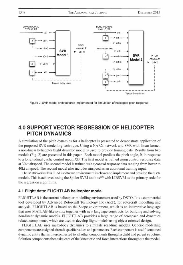
4.0 SUPPORT VECTOR REGRESSION OF HELICOPTER PITCH DYNAMICSA simulation of the pitch dynamics for a helicopter is presented to demonstrate application of the proposed SVR modelling technique. Using a NARX network and SVR with linear kernel, a non-linear helicopter flight dynamic model is used to provide training data. Results from two models (Fig. 2) are presented in this paper. Each model predicts the pitch angle, θ, in response to a longitudinal cyclic control input, XB. The first model is trained using control response data at 30kt airspeed. The second model is trained using control response data ranging from hover to 40kt airspeed. The second model also includes airspeed as an additional training input.

The MathWorks MATLAB software environment is chosen to implement and develop the SVR models. This is achieved using the Spider SVM toolbox(24) with LIBSVM as the primary code for the regression algorithms.

4.1 Flight data: FLIGHTLAB helicopter model

FLIGHTLAB is the current helicopter-modelling environment used by DSTO. It is a commercial tool developed by Advanced Rotorcraft Technology Inc (ART), for rotorcraft modelling and analysis. FLIGHTLAB is based on the Scope environment, which is an interpretive language that uses MATLAB-like syntax together with new language constructs for building and solving non-linear dynamic models. FLIGHTLAB provides a large range of aerospace and dynamics related components, which are used to develop flight models using object oriented design.

FLIGHTLAB uses multi-body dynamics to simulate real-time models. Generic modelling components are assigned aircraft specific values and parameters. Each component is a self-contained dynamic entity that is interconnected to all other components through a child and parent structure. Solution components then take care of the kinematic and force interactions throughout the model.

Figure 2. SVR model architectures implemented for simulation of helicopter pitch response.


A conventional medium sized twin-engine helicopter (refer to Fig. 3), with counter clockwise rotating rotor, was developed in the FLIGHTLAB environment. This non-linear, six degree-of-freedom, rigid body model was used previously for Human-in-the-Loop Simulator Fidelity trials at DSTO(25). It uses a blade element model for the main rotor, and a disk rotor model for the tail rotor. The model provides a source of noiseless data, which is highly amenable to the development of SVR modelling techniques. Table 2 provides a brief list of the major model parameters. The FLIGHTLAB model provides data at 180Hz, which is then reduced to 10Hz when training the SVR model.

4.2 Method: SVR training and validation

The training data is scaled so that its mean and standard deviation are equal to one. Although not necessarily required, the normalisation of training data avoids certain inputs having more influence than others. This is particularly important when input variables have vastly different ranges, such as angles in radians and velocity in knots. It also allows some consistency in the choice of hyper-parameters ε and C when using different datasets, which would otherwise require

Table 2FLIGHTLAB helicopter parameters

Rotor parameters Main rotor Tail rotorRadius (ft) 26.7 5.2Chord (ft) 2.1 UnknownNo. of blades 4 4Rotor speed (rpm) 256 1,232Rotor twist (deg) ‒12 ‒14Aerofoil type NACA 23012 Unknown

Weight 20,400lbEngine type 2 x turboshaftEngine power 2,800SHP

Control system Rate based, with attitude stabilisationLongitudinal cyclic range 0 to 100%(+’ve nose up)

Figure 3. Representative conventional helicopter.


more specific choices.

. . . (10)

the regularisation coefficient, C, controls the trade off between training error and model complexity. A small value will increase the training errors, while a large value will lead to minimal training errors and a stronger correlation with the training data at the expense of generalisation (referred to from hereon as hard margin behaviour). It is noted from the literature(26) that the value of C seems to have negligible effect when the insensitivity factor, ε, is well chosen. Values of C in this paper are varied from 0.01 to 1,000.

The insensitivity parameter, ε, determines the level of training accuracy for the SVM by controlling the width of the ε-insensitive zone. If ε is larger than the range of the target values, then fewer support vectors are chosen. If ε is set to zero, hard margin behaviour is expected. Generally, the value of ε should increase when greater noise levels are present in the data. A good initial selection is to set ε to the accuracy desired. This is generally a trial and error approach dependent on the noise and range of the data values. Values of ε in this paper are varied from 0.0001 to 1, which is a typically useable range with normalised data.

Quantitative validation is conducted by measuring the mean quadratic loss (MQL) with comparison to the FLIGHTLAB output. A validation data set is then used as a method of both kernel parameter selection and performance testing.

. . . (11)

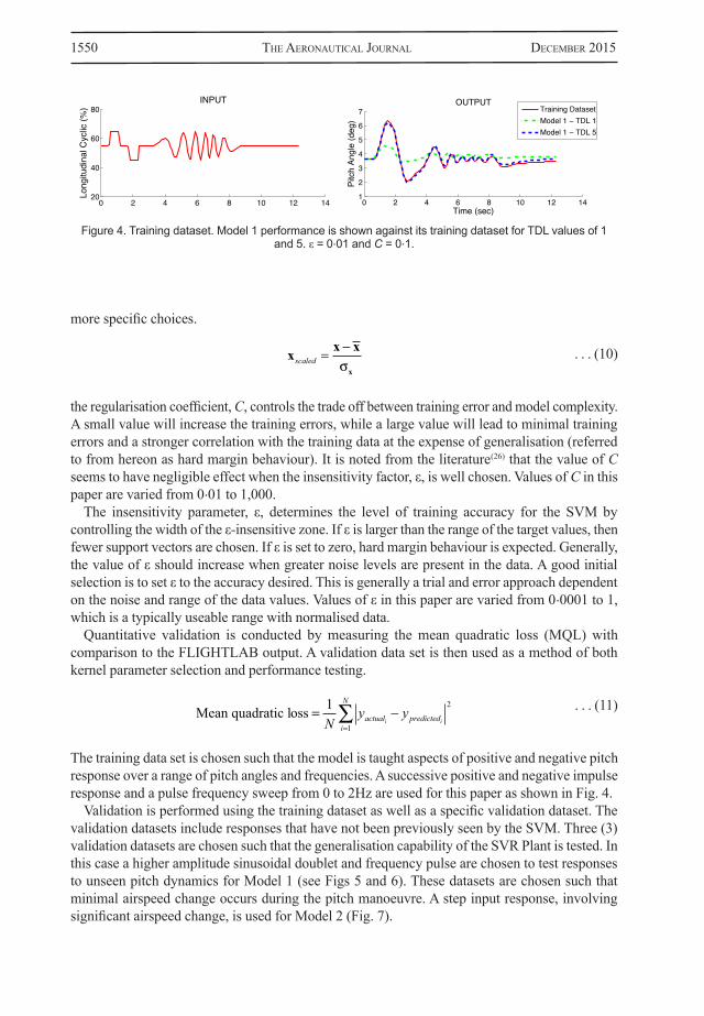
The training data set is chosen such that the model is taught aspects of positive and negative pitch response over a range of pitch angles and frequencies. A successive positive and negative impulse response and a pulse frequency sweep from 0 to 2Hz are used for this paper as shown in Fig. 4.

Validation is performed using the training dataset as well as a specific validation dataset. The validation datasets include responses that have not been previously seen by the SVM. Three (3) validation datasets are chosen such that the generalisation capability of the SVR Plant is tested. In this case a higher amplitude sinusoidal doublet and frequency pulse are chosen to test responses to unseen pitch dynamics for Model 1 (see Figs 5 and 6). These datasets are chosen such that minimal airspeed change occurs during the pitch manoeuvre. A step input response, involving significant airspeed change, is used for Model 2 (Fig. 7).

0 2 4 6 8 10 12 1420

40

60

80INPUT

Long

itudi

nal C

yclic

(%)

0 2 4 6 8 10 12 141

2

3

4

5

6

7OUTPUT

Pitc

h An

gle

(deg

)

Time (sec)

Training DatasetModel 1 − TDL 1Model 1 − TDL 5

0 2 4 6 8 10 12 1420

40

60

80INPUT

Long

itudi

nal C

yclic

(%)

0 2 4 6 8 10 12 141

2

3

4

5

6

7OUTPUT

Pitc

h An

gle

(deg

)

Time (sec)

Training DatasetModel 1 − TDL 1Model 1 − TDL 5

Figure 4. Training dataset. Model 1 performance is shown against its training dataset for TDL values of 1 and 5. ε = 0.01 and C = 0.1.

x x x

xscaled

Mean quadratic loss 1 2

1Ny yactual predicted

i

N

i i


For the validation process, the initial conditions and input profile are chosen to begin the simulation. The initial conditions are used to begin the SVR prediction process where every subsequent time step builds upon the previous prediction of the SVR model. The predictions are then compared using MQL to the dynamic response of the FLIGHTLAB model that also began with the same initial conditions and input profile.

0 1 2 3 4 5 6 7 820

40

60

80INPUT

Long

itudi

nal C

yclic

(%

)

0 1 2 3 4 5 6 7 8−5

0

5

10

15OUTPUT

Pitc

h A

ngle

(de

g)

Time (sec)

Validation Dataset 1Model 1 − TDL 5

0 2 4 6 8 1020

40

60

80INPUT

Long

itudi

nal C

yclic

(%

)

0 2 4 6 8 102

3

4

5

6

7OUTPUT

Pitc

h A

ngle

(de

g)

Time (sec)

Validation Dataset 2Model 1 − TDL 5

0 5 10 15 2020

40

60

80INPUT

Long

itudi

nal C

yclic

(%

)

0 5 10 15 2030

35

40

45

Airs

peed

(K

ts)

Time (sec)

0 5 10 15 20−1

0

1

2

3

4

5

6OUTPUT

Pitc

h A

ngle

(de

g)

Time (sec)

Validation Dataset 3

Model 1 − TDL 5

Model 2 − TDL 5

Figure 5. Validation dataset 1. Model 1 performance is shown against unseen data for a TDL value of 5.

ε = 0.01 and C = 0.1.

Figure 6. Validation dataset 2. Model 1 performance is shown against unseen data for a TDL value of 5.

ε = 0.01 and C = 0.1.

Figure 7. Validation dataset 3. Performance of Model 2 is shown against unseen data for a TDL value of 5. For comparison, Model 1 results are also presented. ε = 0.01 and C = 0.1.


5.0 RESULTS

5.1 SVR Model 1: Pitch response

An SVR model was developed to predict pitch angle response to a longitudinal control input at an airspeed of 30kt. The model was trained using data at 10Hz resolution. A linear kernel with a NARX network was developed as shown for Model 1 in Fig. 2. One training dataset (Fig. 4), and two validation datasets (Figs 5 and 6) were used. This model required three variables to be defined. These included the SVM related insensitivity factor, ε, the regularisation coefficient, C, and the NARX related number of TDLs.

The MQL predictive error and pitch angle prediction (Fig. 8 and Fig. 4 respectively) demon-strate the effect in choice of TDL on the performance of the SVR when compared to both the original training data and the validation datasets. Good performance can be achieved provided that

0 2 4 6 8 1010

−3

10−2

10−1

100

101

TDL

MQ

L er

ror

TrainingValidation

10−4

10−2

100

10−2

100

102

104

10−2

100

102

��

��

��

Figure 8. Model 1 MQL predictive error against the training and validation datasets with variation in TDL.

ε = 0.01 and C = 0.1. Validation dataset 1 & 2 are used.

Figure 9. Model 1 MQL predictive error against the training dataset. Variation in ε = 0.0001:1 and C =

0.01:1000, TDL = 5.

10−4

10−2

100

10−2

100

102

104

10−2

100

102

��

��

��

10−4

10−2

100

10−2

100

102

104

0

200

400

600

��

��

Figure 10. Model 1 MQL predictive error against the validation datasets 1&2. Variation in ε = 0.0001:1

and C = 0.01:1000, TDL = 5.

Figure 11. Model 1 Number of support vectors produced after training. Variation in ε = 0.0001:1

and C = 0.01:1000, TDL = 5.


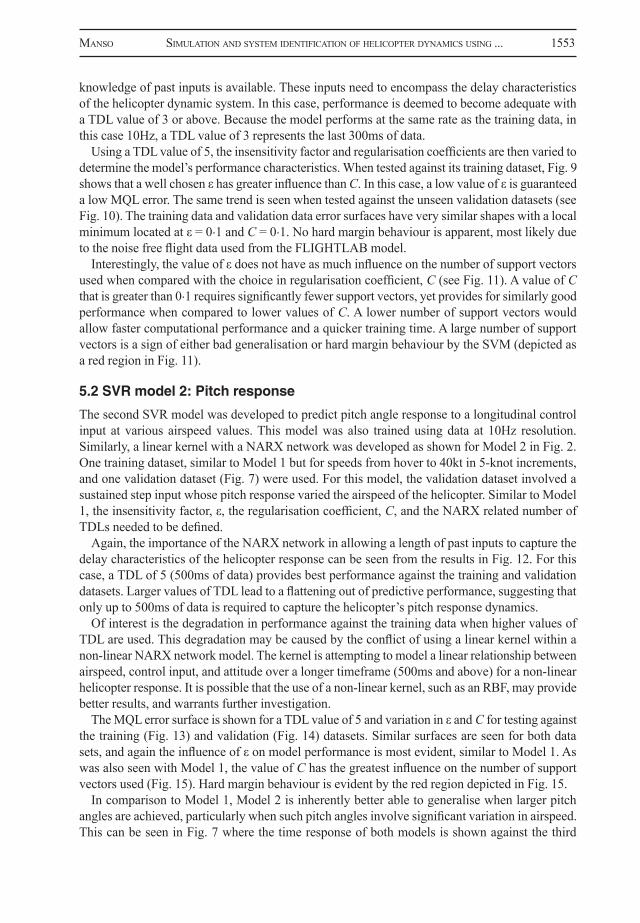
knowledge of past inputs is available. These inputs need to encompass the delay characteristics of the helicopter dynamic system. In this case, performance is deemed to become adequate with a TDL value of 3 or above. Because the model performs at the same rate as the training data, in this case 10Hz, a TDL value of 3 represents the last 300ms of data.

Using a TDL value of 5, the insensitivity factor and regularisation coefficients are then varied to determine the model’s performance characteristics. When tested against its training dataset, Fig. 9 shows that a well chosen ε has greater influence than C. In this case, a low value of ε is guaranteed a low MQL error. The same trend is seen when tested against the unseen validation datasets (see Fig. 10). The training data and validation data error surfaces have very similar shapes with a local minimum located at ε = 0.1 and C = 0.1. No hard margin behaviour is apparent, most likely due to the noise free flight data used from the FLIGHTLAB model.

Interestingly, the value of ε does not have as much influence on the number of support vectors used when compared with the choice in regularisation coefficient, C (see Fig. 11). A value of C that is greater than 0.1 requires significantly fewer support vectors, yet provides for similarly good performance when compared to lower values of C. A lower number of support vectors would allow faster computational performance and a quicker training time. A large number of support vectors is a sign of either bad generalisation or hard margin behaviour by the SVM (depicted as a red region in Fig. 11).

5.2 SVR model 2: Pitch response

The second SVR model was developed to predict pitch angle response to a longitudinal control input at various airspeed values. This model was also trained using data at 10Hz resolution. Similarly, a linear kernel with a NARX network was developed as shown for Model 2 in Fig. 2. One training dataset, similar to Model 1 but for speeds from hover to 40kt in 5-knot increments, and one validation dataset (Fig. 7) were used. For this model, the validation dataset involved a sustained step input whose pitch response varied the airspeed of the helicopter. Similar to Model 1, the insensitivity factor, ε, the regularisation coefficient, C, and the NARX related number of TDLs needed to be defined.

Again, the importance of the NARX network in allowing a length of past inputs to capture the delay characteristics of the helicopter response can be seen from the results in Fig. 12. For this case, a TDL of 5 (500ms of data) provides best performance against the training and validation datasets. Larger values of TDL lead to a flattening out of predictive performance, suggesting that only up to 500ms of data is required to capture the helicopter’s pitch response dynamics.

Of interest is the degradation in performance against the training data when higher values of TDL are used. This degradation may be caused by the conflict of using a linear kernel within a non-linear NARX network model. The kernel is attempting to model a linear relationship between airspeed, control input, and attitude over a longer timeframe (500ms and above) for a non-linear helicopter response. It is possible that the use of a non-linear kernel, such as an RBF, may provide better results, and warrants further investigation.

The MQL error surface is shown for a TDL value of 5 and variation in ε and C for testing against the training (Fig. 13) and validation (Fig. 14) datasets. Similar surfaces are seen for both data sets, and again the influence of ε on model performance is most evident, similar to Model 1. As was also seen with Model 1, the value of C has the greatest influence on the number of support vectors used (Fig. 15). Hard margin behaviour is evident by the red region depicted in Fig. 15.

In comparison to Model 1, Model 2 is inherently better able to generalise when larger pitch angles are achieved, particularly when such pitch angles involve significant variation in airspeed. This can be seen in Fig. 7 where the time response of both models is shown against the third


validation data set. Here, Model 2 is better able to predict the reduction in pitch angle over time, although not to the same level as the validation data.

6.0 APPLICATION WITH FLIGHT TEST DATAA small selection of flight test data recorded at 20Hz from a Sikorsky Seahawk helicopter is provided for training and testing of the SVR model. The data was recorded during the 1994 ADF airborne trials of the S-70B2 helicopter and is provided courtesy of the Aircraft Maintenance and Flight Trials Unit (AMAFTU). The training (Fig. 16) and validation (Fig. 17) datasets show pitch response to longitudinal cyclic input at hover conditions. Although the datasets are very small, this data provides an opportunity to train an SVR model using noisy data. Because only hover pitch response data was provided without airspeed, the Model 1 NARX architecture was used.

Best performance against the validation dataset represents a TDL of 8, corresponding to 400ms of historic data. In this case, increasing level of TDL does not aid in performance against the

0 2 4 6 8 1010

−2

10−1

100

101

TDL

MQ

L er

ror

TrainingValidation

10−4

10−2

100

10−2

100

102

104

10−2

100

102

��

��

��

Figure 12. Model 2 MQL predictive error against the training and validation datasets with variation in TDL.

ε = 0.01 and C = 0.1. Validation dataset 3 is used.

Figure 13. Model 2 MQL predictive error against the training dataset. Variation in ε = 0.0001:1 and

C = 0.01:1000, TDL = 5.

10−4

10−2

100

10−2

100

102

104

10−2

100

102

��

��

��

10−4

10−2

100

10−2

100

102

104

0

1000

2000

3000

��

��

Figure 14. Model 2 MQL predictive error against validation dataset 3. Variation in ε = 0.0001:1 and

C = 0.01:1000, TDL = 5.

Figure 15. Model 2 number of support vectors produced after training. Variation in ε = 0.0001:1

and C = 0.01:1000, TDL = 5.


unseen validation data (see Fig. 18). To aid in comparison with previous results, a TDL value of 10 (500ms) is used for simulation here. Note that higher values of TDL with the training dataset do not lead to a levelling out of performance. This may be a sign of limited number of training data points with which to achieve good generalisation, because levelling of performance is clearly seen with the validation dataset.

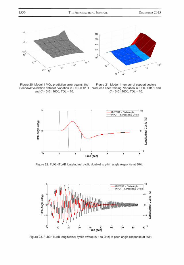
The MQL predictive error surface against the training dataset (Fig.19) is very similar to the previous models taught with noiseless FLIGHTLAB data. In this case, a low value for ε and C provide the best performance against the validation data (Fig. 20), even though the number of support vectors required show hard margin behaviour (depicted as the red region in Fig. 21). Better results may have been achieved with the availability of airspeed data or a larger number of data points.

0 0.5 1 1.5 2 2.5 3 3.5 450

60

70

80INPUT

Long

itudi

nal C

yclic

(%

)

0 0.5 1 1.5 2 2.5 3 3.5 41

2

3

4

5

6OUTPUT

Pitc

h A

ngle

(de

g)

Time (sec)

Training Dataset − Seahawk

Model 1 − Seahawk − TDL 1


0 0.5 1 1.5 2 2.5 3 3.5 450

60

70

80INPUT

Long

itudi

nal C

yclic

(%

)

0 0.5 1 1.5 2 2.5 3 3.5 44

6

8

10

12OUTPUT

Pitc

h A

ngle

(de

g)

Time (sec)

Validation Dataset − Seahawk


Figure 16. Training dataset. Model 1 Performance is shown against Seahawk helicopter training data for

TDL values of 1 and 10. ε = 0.01 and C = 0.1.

Figure 17. Validation dataset. Model 1 Performance is shown against unseen Seahawk helicopter data for

a TDL value of 10. ε = 0.01 and C = 0.1.

0 5 10 15 2010

−3

10−2

10−1

100

101

102

TDL

MQ

L er

ror

TrainingValidation

10−4

10−2

100

10−2

100

102

104

10−2

100

102

��

��

��

Figure 18. Model 1 MQL predictive error against Seahawk training and validation datasets with

variation in TDL. ε = 0.01 and C = 0.1.

Figure 19. Model 1 MQL predictive error against the Seahawk training dataset. Variation in ε = 0.0001:1

and C = 0.01:1000, TDL = 10.


10−4

10−2

100

10−2

100

102

104

10−2

100

102

��

��

��

10−4

10−2

100

10−2

100

102

104

0

200

400

600

800

��

��

Figure 20. Model 1 MQL predictive error against the Seahawk validation dataset. Variation in ε = 0.0001:1

and C = 0.01:1000, TDL = 10.

Figure 21. Model 1 number of support vectors produced after training. Variation in ε = 0.0001:1 and

C = 0.01:1000, TDL = 10.

0 1 2 3 4 5 6−5

0

5

Time (sec)

Pitc

h A

ngle

(de

g)

0 1 2 3 4 5 6−10

0

10

Time (sec)

Long

itudi

nal C

yclic

(%

)

OUTPUT − Pitch AngleINPUT − Longitudinal Cyclic

Figure 22. FLIGHTLAB longitudinal cyclic doublet to pitch angle response at 30kt.

0 10 20 30 40 50 60 70 80 90−4

−2

0

2

4

Time (sec)

Pitc

h A

ngle

(de

g)

0 10 20 30 40 50 60 70 80 90−10

−5

0

5

10

Time (sec)

Long

itudi

nal C

yclic

(%

)

OUTPUT − Pitch AngleINPUT − Longitudinal Cyclic

Figure 23. FLIGHTLAB longitudinal cyclic sweep (0.1 to 2Hz) to pitch angle response at 30kt.


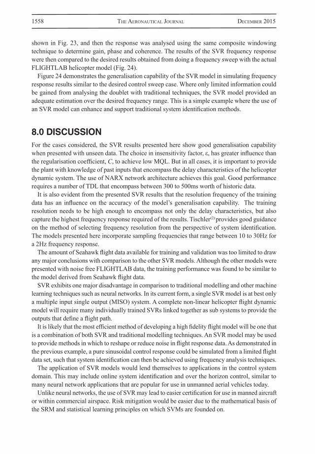
7.0 APPLICATION TO FREQUENCY RESPONSEAn example of the application of SVR modelling is in the domain of filtering and augmentation of flight data for traditional system identification and analysis. Take an example where a control frequency response is required in the region of 0.1 to 2Hz (representing typical pilot control), but due to operational limitations only a doublet control response is achieved. For this example, the FLIGHTLAB helicopter model is used as the aircraft to be analysed.

Figure 22 depicts the control response achieved with a doublet at 30kt airspeed. Compare this to the desired control sweep response in Fig. 23. Undertaking a frequency response analysis of the doublet using a composite Hanning windowing technique(2), the gain, phase and coherence is shown in Fig. 24. This doublet response was used as a training data set for a Model 1 based SVR model with 30Hz resolution, TDL of 15 (500ms), ε of 0.01, and C of 100. Subsequently, the SVR model was used to simulate the response to the longitudinal cyclic frequency sweep

10−1

100

−40

−35

−30

−25

−20

−15

Frequency (Hz)

Mag

nitu

de (

dB)

SVR − SweepFLIGHTLAB − SweepFLIGHTLAB − Doublet

Figure 24. Composite Hanning frequency analysis for FLIGHTLAB (doublet and sweep) and SVR (sweep) pitch attitude to longitudinal cyclic response at 30kt.

10−1

100

−300

−250

−200

−150

−100

−50

0

Frequency (Hz)

Pha

se [d

eg]

10−1

100

0

0.2

0.4

0.6

0.8

1

1.2

Frequency (Hz)

Coh

eren

ce


shown in Fig. 23, and then the response was analysed using the same composite windowing technique to determine gain, phase and coherence. The results of the SVR frequency response were then compared to the desired results obtained from doing a frequency sweep with the actual FLIGHTLAB helicopter model (Fig. 24).

Figure 24 demonstrates the generalisation capability of the SVR model in simulating frequency response results similar to the desired control sweep case. Where only limited information could be gained from analysing the doublet with traditional techniques, the SVR model provided an adequate estimation over the desired frequency range. This is a simple example where the use of an SVR model can enhance and support traditional system identification methods.

8.0 DISCUSSIONFor the cases considered, the SVR results presented here show good generalisation capability when presented with unseen data. The choice in insensitivity factor, ε, has greater influence than the regularisation coefficient, C, to achieve low MQL. But in all cases, it is important to provide the plant with knowledge of past inputs that encompass the delay characteristics of the helicopter dynamic system. The use of NARX network architecture achieves this goal. Good performance requires a number of TDL that encompass between 300 to 500ms worth of historic data.

It is also evident from the presented SVR results that the resolution frequency of the training data has an influence on the accuracy of the model’s generalisation capability. The training resolution needs to be high enough to encompass not only the delay characteristics, but also capture the highest frequency response required of the results. Tischler(2).provides good guidance on the method of selecting frequency resolution from the perspective of system identification. The models presented here incorporate sampling frequencies that range between 10 to 30Hz for a 2Hz frequency response.

The amount of Seahawk flight data available for training and validation was too limited to draw any major conclusions with comparison to the other SVR models. Although the other models were presented with noise free FLIGHTLAB data, the training performance was found to be similar to the model derived from Seahawk flight data.

SVR exhibits one major disadvantage in comparison to traditional modelling and other machine learning techniques such as neural networks. In its current form, a single SVR model is at best only a multiple input single output (MISO) system. A complete non-linear helicopter flight dynamic model will require many individually trained SVRs linked together as sub systems to provide the outputs that define a flight path.

It is likely that the most efficient method of developing a high fidelity flight model will be one that is a combination of both SVR and traditional modelling techniques. An SVR model may be used to provide methods in which to reshape or reduce noise in flight response data. As demonstrated in the previous example, a pure sinusoidal control response could be simulated from a limited flight data set, such that system identification can then be achieved using frequency analysis techniques.

The application of SVR models would lend themselves to applications in the control system domain. This may include online system identification and over the horizon control, similar to many neural network applications that are popular for use in unmanned aerial vehicles today.

Unlike neural networks, the use of SVR may lead to easier certification for use in manned aircraft or within commercial airspace. Risk mitigation would be easier due to the mathematical basis of the SRM and statistical learning principles on which SVMs are founded on.


9.0 CONCLUSIONS AND FURTHER WORKThe SVR model results show significant promise in the ability to represent aspects of a helicop-ter’s attitude response at a high fidelity. To achieve this, it is important to provide the model with knowledge of past inputs that encompass the delay characteristics of the helicopter dynamic system. In this case, the use of NARX network architecture achieves this goal. For the cases considered, good performance requires a number of tapped delay lines (TDL) that encompass between 300 to 500ms worth of historic data.

The SVR models presented here have only modelled the response in the primary axis, therefore further work may be beneficial in the area of off-axis response. Further work is also recommended to investigate the SVR generalisation capability under varying data sampling frequencies, and when appreciable noise is evident in the flight data.

ACKNOWLEDGEMENTSThe author wishes to thank the Aircraft Maintenance and Flight Trials Unit (AMAFTU) of the ADF for their permission to use Seahawk flight data in this paper.

REFERENCES1. AllerTon, D. Flight models for FTDs, RAeS Flight Simulation Conference, The Future of Flight Training

Devices 12-13 November 2014, London, UK.2. Tischler, m.b. and remple, r.K. Aircraft and rotorcraft system identification, engineering methods

with flight test examples, AIAA, 2006.3. smolA, A.J. and scholKopf, b. A tutorial on support vector regression, Statistics and Computing, 2004,

14, pp 199-222.4. VApniK, V.N. The Nature of Statistical Learning Theory, 1995, Springer-Verlag, New York, USA.5. osunA, E. Applying SVMs to face detection, IEEE Intelligent Systems, July/August 1998, 13, (4), pp

23-26.6. DumAis, S. Using SVMs for text categorization, IEEE Intelligent Systems, July/August 1998, 13, (4),

pp 21-23.7. AbrAhAm, A., philip, n. and sArATchAnDrAn, p. Modeling chaotic behavior of stock indices using

intelligent paradigms, Int J Neural, Parallel & Scientific Computations, 2003, 11, pp 143-160.8. fAn, h., DuliKrAVich, g. and hAn, Z. Aerodynamic data modeling using support vector machines,

Inverse Problems in Sci and Eng, June 2005, 13, (3), pp 261-278.9. scholKopf, b., sung, K., burges, c., girosi, f., niyogi, p., poggio, T. and VApniK, V. Comparing support

vector machines with Gaussian kernels to radial basis function classifiers, IEEE Transactions on Signal Processing, November 1997, pp 2758-2765.

10. muKherJee, s., osunA, e. and girosi, f. Nonlinear prediction of chaotic time series using support vector machines, IEEE Neural Networks for Signal Processing, 1997, pp 511-520.

11. VApniK, V.N. An overview of statistical learning theory, IEEE Transactions on Neural Networks, September 1999.

12. gunn, S. Support vector machines for classification and regression, University of Southampton, 10 May 1998.

13. plATT, J. How to implement SVMs, IEEE Intelligent Systems, July/August 1998, 13, (4), pp 26-28.14. muller, K., miKA, s., rATsch, g., TsuDA, K. and scholKopf, b. An introduction to kernel-based learning

algorithms, IEEE Transactions on Neural Networks, March 2001, 12, (2), pp 181-201.15. scholKopf, B. SVMs — a practical consequene of learning theory, IEEE Intelligent Systems, July/August

1998, 13, (4), pp 18-21.16. AnguiTA, D., boni, A. and riDellA, s. A digital architecture for support vector machines: Theory, algorithm,

and FPGA implementation, IEEE Transactions on Neural Networks, September 2003, 14, (5).17. bellmAn, R.E. Dynamic Programming, 1957, Rand Corporation, Princeton University Press.


18. pADfielD, G. Helicopter Flight Dynamics: The Theory and Application of Flying Qualities and Simulation Modeling, 1999, AIAA education series.

19. bhAnDAri, s., chen, b., colgren, r. and chen, X. Application of support vector machines to the modeling and control of a UAV helicopter, AIAA Modeling and Simulation Technologies Conference and Exhibition, 20-23 August 2007, Hilton Head, SC, USA.

20. muDigere, D., omKAr, s. and KumAr, m. Identification of helicopter dynamics based on flight data using a PSO driven recurrent neural network model, AHS 64th Annual Forum, 29 April 29-1 May 2008, Montreal, Canada.

21. KumAr, m., omKAr, s., gAnguli, r., sAmpATh, p. and suresh, s. Identification of helicopter dynamics using recurrent neural networks and flight data, AHS 59th Annual Forum, 6-8 May 2003, Phoenix, AZ, USA.

22. nArenDrA, K. and pArThAsArAThy, K. Identification and control of dynamical systems using neural networks, IEEE Transactions on Neural Networks, 1990, 1, (1), pp 4-27.

23. mAnso, S. Support Vector Regression of a High Fidelity Helicopter Flight Model, PhD thesis, August 2008, RMIT University, Australia.

24. WesTon, J., elisseeff, A., bAKir, g. and sinZ, f. http://www.kyb.tuebingen.mpg.de/bs/people/spider/ index.html

25. mAnso, s. and bourne, K. Assessing the fidelity of a human-in-the-loop helicopter flight research simulator, AHS 70th Annual Forum, 20–22 May 2014, Montreal, Quebec, Canada.

26. cherKAssKy, V. and mA, y. Selection of meta-parameters for support vector regression, ICANN 2002, 2002, pp 687-693.

Simulation and system identification of helicopter ... · regression in the domain of simulation...

Documents

Transcript of Simulation and system identification of helicopter ... · regression in the domain of simulation...