1

Abstract: Development of a reliable high-performance helicopter-based unmanned aerialvehicle (UAV) requires an accurate and practical model of the vehicle dynamics. This reportdescribes the process and results of the dynamic modeling of a model-scale unmanned helicopter(Yamaha R-50 with 10 ft rotor diameter) using system identification. A complete dynamic modelwas derived for both hover and cruise flight conditions. In addition to standard helicopter flightcharacteristics, the model explicitly accounts for the stabilizer bar, which has a strong influence onthe flight dynamics and is widely used in model-scale helicopters. The accuracy of the developedmodel is verified by the comparison between predicted and actual responses from the model andthe flight experiments (in both frequency and time domains), and between key identifiedparameters and their theoretical values. Scaling of the main characteristics of the R-50 model-scale helicopter with respect to those of a UH-1H full-size helicopter was performed to determinehow the size influences the flight dynamics of helicopters.

System Identification Modelingof a Model-Scale Helicopter

Bernard Mettler and Takeo KanadeThe Robotics Institute

Carnegie Mellon UniversityPittsburgh, Pennsylvania

Mark B. TischlerArmy/NASA Rotorcraft DivisionAeroflightdynamics Directorate

Ames Research Center

CMU-RI-TR-00-03

2

1 Introduction

Model-scale helicopters are increasingly popular platforms for unmanned aerial vehicles(UAVs). The ability of helicopters to take off and land vertically, to perform hover flight aswell as cruise flight, and their agility and controllability, make them ideal vehicles for a rangeof applications which can take place in a variety of environments. Existing model-scalehelicopter-based UAVs (HUAVs), however, exploit only a modest part of the helicopter’sinherent qualities. For example, their operation is generally limited to hover and slow-speedflight, and their control performance is in most cases sluggish. These limitations on HUAVoperation are mainly the consequence of a poor flight control system.

Throughout the 1990’s, most HUAVs used classical control systems such as single-loop PDsystems. The controller parameters are usually tuned manually for a distinct operating point(generally hover flight). This situation is surprising given the abundance of effectivemultivariable controller synthesis methods. One reason for this situation is that mostmultivariable control methods are model-based, and that dynamic models for a particularmodel-scale helicopter are not readily available.

The dynamic models used for controller synthesis or controller optimization have strictrequirements. The model must capture the effects that govern the performance andmaneuverability of the vehicle. High-bandwidth control requires models with high-bandwidthaccuracy. For helicopters, this implies that they must explicitly account for effects such as therotor/fuselage coupling. At the same time the model must be simple enough to be insightfuland practical for the control synthesis.

Using a standard first-principle based modeling approach, considerable knowledge aboutrotorcraft flight dynamics is required to obtain the governing equations, and comprehensiveflight validations and model refinements are necessary before sufficient accuracy is attained.Instead, in the helicopter community a modeling method based on system identification hasbeen developed and successfully used with full-scale helicopters. The experimental nature ofa system-identification based method enables the engineer to recognize the key flight-dynamic characteristics of the vehicle, and thus allows the engineer to concentrate themodeling effort on these characteristics.

Only a few examples of the application of system identification techniques to the modeling ofmodel-scale helicopters exist. The results obtained are limited compared with what isregularly achieved with full-scale helicopters. For example, a low-order model (rigid bodydynamics) was identified using experiments with a rigged helicopter [1], or only thelongitudinal stability and control derivatives were identified [2].

This report describes the first comprehensive application of system identification techniquesto a model-scale helicopter. Both hover and cruise flight conditions have been treated and allthe effects which are important for the performance and maneuverability of a model-scalehelicopter have been captured. The experiments were conducted on Carnegie Mellon’sHUAV, which is based on a Yamaha R-50 model scale helicopter. For the identification, afrequency-domain method developed by the US Army and NASA was used (ComprehensiveIdentification from FrEquency Responses CIFER [3]).

3

The report is organized as follows: In Section 2, we describe the principal physical and flight-mechanical characteristics of the R-50 model-scale helicopter, as well as the instrumentationand on-board systems. In Section 3, we present the fundamentals of the CIFER

identification method. Section 4 describes the flight-testing performed for the collection of theflight-data. In Section 5, we explain the identification process, concentrating on the definitionof the state-space model structure used in the identification. In Section 6, we present theidentification results: first, the agreement between the predicted frequency responses from theidentified model and the actual frequency responses from the flight-data; second the identifiedmodel parameters, along with, when possible, a comparison of their values wtih the valuespredicted by helicopter theory; and finally, the agreement between the predicted and actualtime responses. Then, we present analytical results: first the eigenvalues and dynamic modes,and second a comparison between characteristic parameters of the model-scale helicopter andthose of a full-scale helicopter scaled to the same rotor diameter.

2 Description of the CMU Helicopter

2.1 Yamaha R-50 Helicopter

The Yamaha R-50 helicopter used in the HUAV project at Carnegie Mellon University(CMU) (Figure 1) is a commercially available model-scale helicopter originally designed forremote operated crop-dusting. Because of the adequate payload (20 kg) and the general easeof operation, it has become a platform of choice for research in autonomous flight. Generalphysical characteristics of the R-50 are given in Table 1.

The R-50 uses a two-bladed main rotor with a Bell-Hiller stabilizer bar. The relatively rigidblades are connected to a yoke through individual flapping hinges and elastomeric fittings.The yoke itself is attached to the rotor shaft over a teetering hinge in an under-swungconfiguration, reducing the Coriolis forces and the associated in-plane blade motion. Theteetering motion is also restrained by an elastomer damper/spring. This rotor system differsfrom classical teetering rotors in that it is stiffer and combines teetered and separately hingedblade motion.

The Bell-Hiller stabilizer bar is a secondary rotor consisting of a pair of paddles connected tothe rotor shaft through an unrestrained teetering hinge. It receives the same cyclic controlinput as the main rotor but, due to its different design, it has a slower response than the mainblades and is also less sensitive to airspeed and wind gusts. The stabilizer bar flapping motionis used to generate a control augmentation to the main rotor cyclic input. This augmentation isimplemented by the bell mixing mechanism. From a control theoretical point of view, thecontrol augmentation can be interpreted as a lagged rate (or “pseudo-attitude”) feedback in the

Figure 1 - Instrumented R-50 in hovering flight

4

pitch and roll loops [4]. The low frequency dynamics are stabilized, which substantiallyincreases the phase margin for pilot/vehicle system in the crossover frequency range(1 3− rad/s) [4]. The pseudo-attitude feedback also reduces the response of the aircraft to windgusts and turbulence.

2.2 Scaling Considerations

Stabilizer bars are common in model-scale helicopters because scaling down the helicoptersize increases the sensitivity of the dynamics to control inputs and disturbances, and reducesthe damping provided by the rotor on the angular pitch and roll motions. Rotor-induceddamping arises from the tendency of the rotor disc therefore of the thrust vector to lagbehind the shaft during pitching or rolling motions. This lag produces a moment about thehelicopter’s center of gravity opposite to the rolling or pitching direction and proportional tothe rolling or pitching rate. A smaller rotor has a smaller rotor time constant τ ; therefore, for agiven pitch or roll rate, it will lag less and thus produce less damping.

The R-50 is about 1/5-th the size of an average-size manned helicopter (a scale factor N=5refers to a rotorcraft of 1/5-th the rotor diameter). The rotor time constant τ is a function ofthe non-dimensional blade lock number γ and the rotor speed Ω (τ γ= 16 Ω). A smallrotorcraft has a rotor speed which is about N faster than the full-size counterpart in order toachieve the same blade tip speed. This means that a small rotorcraft has a N times smallerrotor time constant and thus a N smaller rotor induced damping than does its full-sizecounterpart. A smaller time constant also means a larger bandwidth.

Since the stabilizer bar is not used to produce lift, its dynamic characteristics can be adjustedalmost arbitrarily. This property is used in Radio Controlled (RC) helicopters to adjust theflight-dynamic characteristics of the model helicopter to the skills of the pilot.

2.3 HUAV Instrumentation

Carnegie Mellon’s HUAV has a state-of-the-art instrumentation capable of producing highquality flight data. The centerpiece of the helicopter onboard systems is a VME-based on-board flight computer which hosts a Motorola 68060 processor board and a sensor I/O board.All sensors and actuators of the helicopter connect through the I/O board with the exceptionof the inertial measurement unit (IMU), which connects directly to the processor board

Dimensions see Figure (units: mm)

Rotor speed

Tip speed

850 rpm

449 ft/sDry weight

Instrumented (fullpayload capacity)

97 lb

150 lb

Engine type Single cylinder, 2-stroke, watercooled

Flight autonomy 30 minutes

1,130

1,775

3,070

2,655

520

1,080

Table 1 – R-50 Physical Characteristics

5

through a special serial port. The communication to the ground station takes place viawireless Ethernet. This system runs under a VxWorks real-time operating system.

Three linear servo-actuators are used to control the swash-plate, while another actuator is usedto control the pitch of the tail rotor. The dynamics of all the actuators have been identifiedseparately. The engine speed is controlled by a governor which maintains the rotor speedconstant in the face of changing rotor load.

The HUAV uses three navigation sensors:

• a fiber-optic based inertial measurement unit (IMU), which provides measurements of theairframe accelerations a a ax y z, , , and angular rates p q r, , (resolution: 0 002. g and 0 0027. °,data rate: 400Hz)

• a dual frequency differential global positioning system (GPS) (precision: 2cm, updaterate: 4Hz)

• a magnetic compass for heading information (resolution: 0 5. °, update rate: 2Hz)

The IMU is mounted on the side of the aircraft, and the GPS and compass are mounted on thetail. Velocity and acceleration measurements are corrected for the position offset between thehelicopter center of gravity and the GPS, or IMU. A 12-th order Kalman filter running at 100Hz is used to integrate the measurements from the IMU, GPS and compass to produceaccurate estimates of helicopter position, velocity and attitude.

3 Frequency-Domain Identification

Frequency responses fully describe the linear dynamics of a system. When the system hasnonlinear dynamics (to some extent all real physical systems do), system identificationdetermines the describing functions which are the best linear fit of the system response basedon a first harmonic approximation of the complete Fourier series. For the identification, weused a frequency domain method, developed by the U.S. Army and NASA, known as CIFER

(Comprehensive Identification from Frequency Responses) [3]. While CIFER was developedspecifically for rotorcraft applications, it has been successfully used in a wide range of fixedwing and rotary wing, and unconventional aircraft applications [5]. CIFER provides a set ofutilities to support the various steps of the identification process. All the tools are integratedaround a database system which conveniently organizes the large quantity of data generatedthroughout the identification process.

The steps involved in the identification process are:

1. Collection of flight data. The flight-data is collected during special flight experimentsusing frequency sweeps.

2. Frequency response calculation. The frequency response for each input-output pair iscomputed using a Chirp-Z transform. At the same time, the coherence function for eachfrequency response is calculated.

3 . Multivariable frequency domain analysis. The single-input single-output frequencyresponses are conditioned by removing the effects from the secondary inputs. The partialcoherence measures are computed.

4. Window Combination. The accuracy of the low and high frequency ends of the frequencyresponses is improved through optimal combination of frequency responses generatedusing different window lengths.

6

5. State-space identification. The parameters (derivatives) of an a priori-defined state-spacemodel are identified by solving an optimization problem driven by frequency responsematching.

6. Time Domain Verification. The final verification of the model accuracy is performed bycomparing the time responses predicted by the model with the actual helicopter responsescollected from flight experiments using doublet control inputs.

4 Flight Testing: Collection of Flight-Data

High quality flight data is essential to a successful identification. The principal concerns arethe accuracy of the state estimates (i.e., unbiased, disturbance free, no drop outs), theinformation content of the flight data (i.e., whether the measurements contain evidence of allthe relevant flight-dynamic effects), and the compatibility of the flight data with the postulateof linear dynamics used for the modeling. While the accuracy of the state estimates dependson the instrumentation, the information content and compatibility depends on the execution ofthe flight experiments.

The responses of the system to low frequency excitations are important for the identificationof the speed derivatives (0 1 1. − rad/sec) and the responses to high frequency excitations areimportant for the identification of the coupled rotor/fuselage dynamics (8 14− rad/s). Toguarantee that the flight data captures the dominant flight-dynamic effects, a frequency-sweeptechnique is used for the flight testing [6].

By adjusting the magnitude of the excitation, we make sure that the system response remainswithin a region where the dynamics are predominantly linear. Also, it is important to select acalm day to avoid unmeasured inputs.

A key metric to verify that the flight data is satisfactory for the purpose of systemidentification is its coherence. The coherence γ xy (or partial coherence for a multiple-inputmultiple-output system) indicates how well the output y (any of the estimated helicopterstate) is linearly correlated with a particular input x over the examined frequency range. It iscomputed together with the system’s frequency responses, from the cross spectrum Gxy, andthe input and output auto-spectrum Gxx and Gyy respectively (the partial coherence is derivedfrom the conditioned spectrum).

γ xyxy

xx yy

G

G G2

2

1= ≤ (1)

A coherence larger than 0 6. is considered good. A poor coherence can be attributed to a poorsignal-to-noise ratio, nonlinear effects in the dynamics, or the presence of unmeasured inputssuch as wind gusts. The coherence is also used as a weighting function in the frequencydomain cost function used during the identification of the model parameters.

4.1 Flight-Test Procedure

Two series of flight experiments were organized for each the hover-flight and cruise-flightoperating point. For each flight in a series, the pilot applies a frequency sweep controlsequence to one of the four control inputs via the remote control (RC) unit. While doing so heuses the other control inputs to hold the helicopter at the selected operating point. In order togather enough data, the same experiment is repeated several times.

The experiments are conducted open-loop, except for an active yaw damping system, and thestabilizer bar which can be regarded as a dynamic augmentation. An input cross-feed is used

7

by Yamaha between the collective input and the pedal input to compensate for couplingeffects between the heave and yaw dynamics.

A block-diagram representing the augmented R-50 dynamics is shown in Figure 2. The inputsto the system are the four helicopter control inputs (cyclic longitudinal δ lon and lateral δ lat ,cyclic collective δ col and pedal δ ped ) which enter the system via four actuators (threeswashplate actuators GS and one tail actuator GT ). Both the yaw damping system and thestabilizer bar are represented as dynamics augmentations. Only 6 rigid-body fuselage statesare illustrated (the three linear velocities u v w, , and the three angular velocities p q r, , ).

During the time of the experiment, all control inputs (stick inputs) and all helicopter states arerecorded (100Hz sampling rate). Flight-data from the best runs are then concatenated andfiltered (−3dB @ 10Hz) to remove undesired information such as structural vibrations. Asample of hover condition flight-data of the longitudinal and lateral response for twoconcatenated lateral frequency sweeps is shown in Figure 3.

The flight experiments for the hover condition are unproblematic; the helicopter is in theproximity of the pilot and it is relatively easy to hold the operating point.

The cruise-flight experiments are more problematic. We used a fly-over technique: the pilotaccelerates the R-50 for a constant distance until the helicopter is directly overhead. At thatpoint, the pilot starts performing the different piloted sweeps while flying down the airstripand trying to maintain a constant airspeed. We encountered two problems during the cruise-flight experiments. First, it was difficult for the pilot to maintain a precise airspeed because herelied only on the visual sighting for helicopter attitude information. Second, the length of theflight experiment was limited because the helicopter had to be kept in sight.

The record length is critical because it defines the low frequency content of the flight-data(ω πmin = 2 trec ). Low frequency information (0 1 1. − rad/sec) is important for the identification ofquasi-steady derivatives, such as the speed derivatives. With our experimental method, tryingto push the record length degraded the stability of the airspeed. With this tradeoff, by allowingthe airspeeds to vary between 10 and 20m/s we were able to achieve a maximum recordlength of 10s. These issues could be addressed in future experiments by conducting the flighttesting on a paved runway and using an automobile as a chase vehicle, or even by performingclosed-loop computer-controlled flight testing.

Figure 2 – Augmented R-50 dynamics

8

4.2 Flight-Test Results

The frequency responses derived from the hover-flight data and the respective coherencemetrics are depicted in Appendix 2a. All on-axis responses attain a coherence close to unityover most of the critical frequency range where the relevant dynamical effects take place. Forexample, the two on-axis angular rate responses to their respective cyclic inputs achieve agood coherence (≥0 6. ) up to the frequencies of 8 16− rad/s, where the important airframe/rotorcoupling takes place.

The frequency responses derived from the cruise-flight data and the respective coherencemetrics are depicted in Appendix 2b. Here again, all the on-axis responses achieve highcoherence values. The generally high coherence obtained for the key helicopter responsesspeaks for the quality of the helicopter instrumentation, the successfully performed flightexperiments, and the dominantly linear behavior of the helicopter around the tested operatingconditions.

5 Application of System Identification

Using system identification, we want to achieve the best possible fit of the flight-data with amodel that is consistent with the physical knowledge and intuition. The first part of theproblem consists of the derivation of the dynamic equations that will define the state-spacemodel with the unknown parameters. Once this is accomplished, the parameters of the modelcan be identified. Based on the results obtained, the model structure will be refined untilsatisfactory results are achieved. The criteria used for this iteration are: (i) level of frequencyresponse agreement (frequency error costs), (ii) statistical metrics from the model parameters(insensitivity and Cramer Rao percent), (iv) level of agreement of the system’s time responses(time domain verification), and (v) when a specific model parameter has a physical meaning,the level of agreement of the parameter with its theoretical value.

5.1 Building the State-Space Model Structure

The basic equations of motion for a linear model of the helicopter dynamics are derived fromthe Newton-Euler equations for a rigid body that is free to simultaneously rotate and translatein all six degrees of freedom. The external aerodynamic and gravitational forces arerepresented by using a stability derivative form. In the simplest model, no additional states are

. .

Figure 3 – Sample flight data for two concatenated lateral frequency sweeps

9

used, and the control forces produced by the main rotor and tail rotor are expressed by themultiplication of a control derivative and the corresponding control input.

However, a key aspect of helicopter dynamics is the dynamical coupling between the mainrotor (which produces most of the control forces and moments) and the helicopter fuselage.Omitting this coupling effect has been shown to limit the accuracy of the helicopter model inthe medium to high frequency range [7]. Therefore, for high-bandwidth control design or forhandling quality evaluations, it is essential to account for the dynamic coupling between therotor and the fuselage.

To include the rotor/fuselage coupling the rotor dynamics need to be modeled explicitly andthen coupled to the fuselage equation of motions. A standard way to achieve this is thehybrid-model formulation [6] developed originally for full-scale helicopter modeling. Besidesthe rotor, other effects involving additional dynamics sometimes need to be accounted for.Examples are: the actuators; the engine/drive train system; and control augmentations (such asthe active yaw damping system or the stabilizer bar). A more refined model structure hasanother benefit besides accuracy; the model is physically more consistent, i.e., the modelparameters are less lumped and thus physically more meaningful. Our goal was to explicitlymodel the helicopter dynamics by breaking the system down according to the block-diagramin Figure 2.

The frequency responses and coherence measures derived from the flight data provide cuesabout what dynamic effects are dominant in the different parts of the frequency range as wellas dynamic coupling. Good example are the angular responses (roll rate p and pitch rate q) tothe cyclic inputs (lateral input δ lat and longitudinal input δ lon ). The corresponding frequencyresponses, which are illustrated in Appendix 2a and 2b, show a pronounced lightly-dampedsecond-order behavior. This characteristic is present for both the on-axis and the off-axisresponses. The second-order nature of the response results from a dynamical coupling,namely the coupling between the airframe angular motion and the regressive rotor flapdynamics (blade flapping a b, ). The lightly damped characteristic is due to the presence of astabilizer bar [4].

Lateral and Longitudinal Fuselage Dynamic Equations

From the Newton-Euler equations we derive the four equations for the lateral and longitudinallinear and angular fuselage motions:

˙ ( )u w q v r g X u X au a= − + − + +0 0 θ (2)

˙ ( )v u r w p g Y v Y bv b= − + + + +0 0 φ (3)

p L u L v L bu v b= + + (4)

q M u M v M au v a= + + (5)

The external aerodynamic and gravitational forces and moments are formulated in terms ofstability derivatives [8]. For example, the rotor forces are expressed through the rotorderivatives X Ya b, , and the rotor moments through the flapping spring-derivatives L Mb a, .General aerodynamic effects are expressed by speed derivatives such as X Y L L M Mu v u v u v, , , , , .The centrifugal terms in the linear-motion equations, which are function of the trim condition( u v w0 0 0, , ), are relevant only in cruise flight.

Rotor/Stabilizer-Bar Dynamics

The simplest way to represent the rotor dynamics is as a rigid disc which can tilt about thelongitudinal and lateral axis. This motion corresponds to the first harmonic approximation in

10

the Fourier Series description of the rotor flapping equations. The resulting rotor equations ofmotions are two first order differential equations, for the lateral and longitudinal flapping:

τ τ δ δf f a lat lat lon lonb b p B a B B˙ = − − + + + (6)

τ τ δ δf f b lat lat lon lona a q A b A A˙ = − − + + + (7)

In our initial application of system identification to the modeling of the R-50 [9], we weretreating the rotor/stabilizer bar as a lumped system. The resulting model was accurate.However because the stabilizer bar has a major influence on the helicopter’s flight-dynamiccharacteristics, we decided to explicitly model the stabilizer bar system. This will allow betterstudy of the effects of the stabilizer bar during flight control design or handling qualityevaluations.

The stabilizer bar can be regarded as a secondary rotor, attached to the rotor shaft above themain rotor, through an unrestrained teetering hinge. The blades consist of two simple paddles.The stabilizer bar receives cyclic inputs from the swash-plate in a similar way as the mainblades. Because of the teetering hinge and the absence of restraint, the stabilizer bar isvirtually not subject to cross axis effects (the stabilizer bar restoring forces are entirelycentrifugal, resulting in a resonant frequency for the flapping motion which is identical to therotor rotation speed. Therefore, independently of the amount of damping in the system, thephase lag between the control input and the dynamic response is exactly 90°). We can writethe lateral (d ) and longitudinal (c) stabilizer bar dynamic equations using the same equationsas for the single rotor system (Eq. 6-7) but in an uncoupled form:

τ τ δs s lat latd d p D˙ = − − + (8)

τ τ δs s lon lonc c q C˙ = − − + (9)

Where Dlat and Clon are the input derivatives, and τs is the stabilizer bar’s time constant,which is a function of the paddle lock number γ s and the rotor speed Ω .

The stabilizer bar does not exert any forces or moments on the shaft. The bar dynamics arecoupled to the main rotor via the bell mixer. The bell mixer is a mechanical mixer, whichsuperposes a cyclic command proportional to the amount of stabilizer bar flapping to thecyclic commands coming from the swash-plate. The resulting augmented lateral andlongitudinal main rotor cyclic commands can be written as:

δ δlat lat dK d= + and δ δlon lon cK c= + (10)

The gains Kd and Kc are the stabilizer bar gearing, which are functions of the geometry ofthe bell mixer. Applying the Laplace transformation to the stabilizer bar lateral flappingequations (Eq. 8-9) we obtain:

ds

pD

ss

s

lat

slat= −

++

+τ

τ τδ

1 1(11)

which shows that the stabilizer bar does indeed act as a lagged rate feedback.

Using the same tip-path plane model formulation for the single rotor flapping equations, andintroducing the augmented cyclic commands gives:

τ τ δ δf f a lat lat d lon lonb b p B a B K d B˙ ( )= − − + + + + (12)

τ τ δ δf f b lat lat c lon lona a q A b A K c A˙ ( )= − − + + + + (13)

where B Blat lon, and A Alon lat, are the input derivatives, τ f is the main rotor time constant, whichis a function of the main blade lock number γ and the rotor speed Ω . Ba and Ab account forthe cross-coupling effects occurring at the level of the rotor itself.

11

In the final state-space model, the control augmentation is determined through the system’sstates. Therefore, we need to define the derivatives: B B Kd lat d= and A A Kc lon c= . The relationbetween the derivatives and the gearing of the bell-mixer are:

KB

Bd

d

lat

= and KA

Ac

c

lon

= (14)

In reality, since the bell-mixer operates the same way independently of the rotor azimuth, thegearing is the same for both axes. The gearing value was determined experimentally. Thisrelation of Eq. 14 could be used as a constraint between the derivatives Blat and Bd ( Alon andAc ) to reduce the number of unknown parameters. However, since we were not certain aboutour approach to the modeling of the stabilizer bar, we decided to leave them free (we willcompare the identified value to the value obtained experimentally).

Heave Dynamics

The frequency response of the vertical acceleration to collective (az/col in Appendix 2a and

2b), shows that a first order system should adequately capture the heave dynamics. This

agrees with the rigid body equations from the Newton-Euler equations:˙ ( )w v p u q Z w Zw col col= − + + +0 0 δ (15)

The term in parenthesis same as in Eq. 2 and 3 corresponds to the centrifugal forces that a

relevant for the cruise conditions. Note that the response does not exhibit the peak in

magnitude caused by the inflow effects, typical of full-size helicopters. This is because the

flap frequency for the R-50 (1/rev= 89 rad/s) is well beyond the frequency range of

identification and of piloted excitation (30 rad/s).Yaw Dynamics

The yaw dynamics of the bare helicopter airframe can usually be modeled as the simple firstorder system:

r N

s Nped

ped

rδ=

−(16)

where Nr is the bare airframe yaw damping coefficient and Nped is the sensitivity to the pedalcontrol.

However, in our case, an artificial yaw damping system was used during the flight testing andwe would like to explicitly account for this dynamic augmentation.

Our yaw damping system is obtained through a yaw-rate feedback. Since, at the time of theflight experiment, only the pilot pedal input δ ped and the helicopter yaw rate r were measured,ground experiments were performed to isolate the dynamics of the tail actuator and yaw rategyro. The dynamics of the actuator and rate gyro were described by their respective frequencyresponses Tact and Tgyro . By expressing the yaw dynamics of the bare airframe as the frequencyresponse Trδ , we can formulate the frequency response of the augmented yaw dynamics as:

TT T

T T Tr aug

r act

r act gyroδ

δ

δ, =

+1(17)

Since Tr augδ , is known from the flight experiments we can solve for the unknown bare airframedynamics Trδ using frequency response arithmetic.

12

TT

T T T Tr

r aug

act r aug act gyroδ

δ

δ=

−,

,

(18)

The resulting frequency response for the bare airframe yaw dynamics Trδ did not exhibit thefirst order form of Eq. 16. From this we conclude that other dynamic effects, such as theengine drive-train dynamics, influence the yaw dynamics.

To avoid increasing the complexity of the model, we decided to revert to the representationwe used in [9]. There, we assume that the augmented yaw dynamics could be modeled as thefirst order bare airframe dynamics with a yaw rate feedback represented by a simple firstorder low-pass filter:

r

r

K

s Kfb r

rfb

=+

(19)

The closed loop transfer function for the augmented yaw rate response becomes:r N s K

s K N s K N N Kped

ped rfb

rfb r r ped r rfbδ=

++ − + −

( )

( ) ( )2 (20)

With the corresponding differential equations used in the state-space model:

˙ ( )r N r N rr ped ped fb= + −δ (21)

r K r K rfb rfb fb r= − + (22)

Again, since we have only the measurements of the pilot input δ ped and the yaw rate r , theabove representation is over-parameterized. One constraint between two parameters must beadded in order to avoid having problems during the identification due to correlatedparameters. As constraint, we stipulate that the pole of the low-pass filter must be twice asfast as the pole of the bare airframe yaw dynamics:

K Nrfb r= − ⋅2 (23)

With this constraint, a low transfer function cost is attained. However the value obtained forthe bare airframe yaw damping Nr, is not necessarily physically meaningful. However, thisshould not constitute a big limitation since the active yaw damping system can be retained infuture flight control designs as part of the bare airframe dynamics.

Offset Equations

In the speed equations (Eq. 2-3), the derivatives Xa and Yb should theoretically be equalrespectively to plus and minus the value of the gravity (g = 32 2. ft/s2). Enforcing that constraintis possible only if the flight-data has been properly corrected for the position offset in thesensor location relative to the C.G. Since, in our case, the C.G. location is not known withsufficient accuracy, we have explicitly accounted for a vertical offset hcg by relating themeasured speeds (v um m, ) to the speed at the C.G. (v u, ).

v v h pm cg= − (24)

u u h qm cg= + (25)

Using this method, we were able to enforce the constraint − = =X Y ga b , and, at the same time,identify the unknown vertical offset hcg .

Swash-Plate Actuator Dynamics

The swash-plate actuators are used to implement the main rotor collective control input aswell as the cyclic control inputs for the stabilizer bar and the bare rotor. Explicitly modeling

13

the stabilizer bar exposes the fast dynamics of the bare rotor. To allow for an accurateidentification of the fast bare rotor dynamics, the dynamics of the swash-plate actuators mustbe accounted for. The dynamics of the swash-plate actuators were identified during groundexperiments. An accurate fit of their frequency responses was achieved with a first ordertransfer function:

G ss

R ( ) =+15

15 (26)

State-Space Identification

The full state-space model of the R-50 dynamics is obtained by collecting all the differentialequations in a matrix differential equation:

Mx Fx Gu˙ = + (27)

with state vector x and input vector u . The system matrix F contains the stability derivatives,the input matrix G contains the input derivatives, and the M matrix contains the rotor timeconstants for the rotor flapping equations. The full state-space system is depicted in Table 2.

From the coherence measure obtained during the multivariable frequency domain analysis, weselect the frequency responses that should be used for the state-space identification and, foreach response, what frequency range should be used for the fitting. The final structure isobtained by adding and removing derivatives according to the quality of the frequencydomain fit and statistical information about the derivatives. The useful statistics are theinsensitivity of the cost function to each derivative and the correlation between thederivatives. Insensitive and/or correlated parameters are dropped.

A helicopter responds differently in hover flight than it does in cruise flight. We observedthat, for our system, these differences did not significantly affect the model structure, butrather were mostly absorbed in the derivatives. For the cruise flight condition, because of thenon-negligible speed, we had to account for the centrifugal acceleration terms which appear inthe equation of motion of the fuselage’s linear accelerations (Eq. 2-3). The average trimcondition for the forward flight experiments is u0 49 2= . ft/s, v0 11= − ft/s, and w0 0= ft/s. All

˙

˙

˙

˙

˙

˙

˙

˙

˙

˙

˙

˙

˙

u

v

p

q

a

b

w

r

r

c

d

Xu g Xa

Yv g Yb

Lu Lv

f

f

fb

s

s

φ

θ

τ

τ

τ

τ

=

−0 0 0 0 0 0 0 0 0 0

0 0 0 0 0 0 0 0 0 0

00 0 0 0 0 0 0 0 0

0 0 0 0 0 0 0 0 0

0 0 1 0 0 0 0 0 0 0 0 0 0

0 0 0 1 0 0 0 0 0 0 0 0 0

0 0 0 0 0 1 0 0 0 0

0 0 0 0 0 1 0 0 0 0

0 0 0 0 0 0 0 0 0

0 0 0

Lb Lw

Mu Mv Ma Mw

Ab Ac

Ba Bd

Za Zb Zw Zr

Nv N p

f

f

− −

− −

τ

τ

00 0 0 0 0

0 0 0 0 0 0 0 0 0 0 0

0 0 0 0 0 0 0 0 0 0 1 0

0 0 0 0 0 0 0 0 0 0 0 1

Nw Nr Nrfb

Kr Krfb

u

v

p

q

a

b

w

r

s

s

− −

− −

τ

τ

φ

θ

rr

c

d

Yped

Mcol

Alat Alon

Blat Blon

Zcol

N ped Ncol

Clon

Dlat

fb

+

0 0 0 0

0 0 0

0 0 0 0

0 0 0

0 0 0 0

0 0 0 0

0 0

0 0

0 0 0

0 0

0 0 0 0

0 0 0

0 0 0

δ

δ

δ

δ

lat

lon

ped

col

Table 2 – State-space system

14

differences are visible in Appendix 1, which shows the parameter values and associatedstatistics, and in s 3, which shows the costs achieved by each transfer function, and indicateswhich frequency responses are relevant for the two operating conditions.

6 Results and Discussion

6.1 Frequency Response Agreement

The predicted frequency responses from the identified model show a good agreement with thefrequency responses from the flight-data, both in hover and cruise conditions. The transferfunction costs are given in Table 3 and the frequency response comparison is depicted inAppendix 2a and 2b. Compared with the results obtained for the lumped rotor/stabilizer bar[9], the off-axis angular responses (p to δ lon and q to δ lat ) have been significantly improvedby explicitly modeling the stabilizer bar. This close agreement is better than what is usuallyachieved in full-size helicopters. This can be attributed to the dynamics of the model-scalehelicopter being dominated by the rotor dynamics and to the absence of complex aerodynamiceffects.

6.2 Identified Model Parameters

The Table in Appendix 1 gives the numerical values of the identified derivatives and theirassociated accuracy statistics: the Cramer-Rao percent (C.R.%) and the insensitivity (I%) ofthe derivatives. These statistics indicate that all of the key control and response parameters areextracted with a high degree of precision [6]. Notice that most of the quasi-steady derivativeshave been dropped, thus showing that the rotor plays a dominant role in the dynamics ofmodel-scale helicopters. This is also reflected by the number of rotor flapping derivatives ( )b

and ( )a. The term actuated helicopter is a good idealization of the dynamics of the model-scale helicopter, where the rotor dominates the response.

Rotor Parameters

For the hover condition, the identified stabilizer bar and bare rotor time constants came out asrespectively τ s = 0 34. s and τ f = 0 046. s. These values are close to the theoretical values ofτ s = 0 36. s and τ f = 0 053. s, predicted from the lock numbers γ of the respective blades and therotor speed Ω .

Hover Cruise Hover Cruise

VX /LAT 15.741 - Q /LON 41.308 9.696

VY /LAT 18.424 - AX /LON 27.915 48.752

VZ /LAT - 71.105 AY /LON 35.035 -

P /LAT 61.539 12.955 AZ /LON 33.805 44.240

Q /LAT 50.376 18.468 P /COL - 45.835

AX /LAT 15.741 - Q /COL - 19.143

AY /LAT 17.363 23.469 R /COL 35.217 -

R /LAT 27.382 - AZ /COL 55.276 78.184

AZ /LAT 24.969 - AY /PED - 10.278

VX /LON 27.915 - VY /PED - 39.134

VY /LON 35.035 - R /PED 18.841 23.542

VZ /LON - 48.521 AZ /PED 19.406 -

P /LON 37.067 15.555 Average 31.492 33.925

Table 3 – Transfer Function Costs

15

τγ

= 16

Ω(28)

The blade lock number describes the ratio between the aerodynamic and inertial forces actingon the blade.

γ ρ α=−c c R r

Ip

b

( )4 4

(29)

It is defined by the air density ρ , the blade chord length cp , the lift curve slope cα , the insideand outside radii of the blade r , R, and the blade inertia Ib .

For the main blade the effective lock number γ eff was used to account for the inflow effects.

γ γσ να

effc

=+1 16 0

(30)

where σ , is the rotor solidity, and ν0 is the inflow ratio derived from the thrust coefficient(ν0 0 5 0= . cT ).

These results also validate our results from our earlier work, where the main rotor andstabilizer bar were modeled as a lumped system. We can now state that the time constantsidentified at the time (τ =0 38. s) belonged in fact to the stabilizer bar. This shows that thestabilizer bar dominates the rotor response characteristics and behaves like a model followingcontroller.

In cruise condition the rotor time constants decreases to τ s = 0 26. s and τ f = 0 035. s, which is ananticipated result.

The stabilizer bar couples to the main rotor, through the derivatives Bd and Ac . By applyingEquation 14, we can calculate the equivalent bell-mixer gearing. The result of Kd = 10 92. andKc = 12 88. for, respectively, the lateral and longitudinal axes, are close to the real gearingK = 13 58. determined experimentally. In forward flight, the equivalent gearing become:Kd = 10 73. and Kc = 13 79. . Which agrees with the reality that the gearing is constant.

The identified roll and pitch rotor spring derivatives are respectively Lb = 166 1. andMa = 82 57. , for hover conditions. Their values for cruise condition are about 30% larger:Lb = 213 2. and Ma = 108 , which is an expected effect.

The lateral and longitudinal main rotor control derivatives have reasonable values with onlyslight changes between hover and cruise conditions. The only exception is Blon , which is 45%larger in cruise flight, indicating a higher cross axis activity. The stabilizer bar controlderivatives are almost identical for both flight conditions, which validates the idea that theirdesign is aerodynamically neutral.

These physically meaningful results indicate that the hybrid model structure with thestabilizer bar augmentation accurately captures the rotor dynamics and its coupling with thefuselage.

Quasi-Steady Derivatives

The speed derivatives X Yu v, , in the equations (Eq. 2-3), have the sign and relative magnitudesexpected for hovering helicopters, but the absolute magnitudes are all considerably larger (2-5times) than those for full scale aircraft. This is expected from the dynamic scalingrelationships as discussed later. In cruise flight the longitudinal speed derivative Xu increasessignificantly. Note that this derivative has the highest insensitivity of all derivatives (29 6. and27 5. for, respectively, hover and cruise flight), as well as a very high Cramer-Rao percent.

16

Therefore, the identified value is unreliable. This poor result is related to the insufficient lowfrequency information content of the flight data. It can be improved by longer record lengths.

The speed derivatives Lu , Lv and Mu , Mv in the angular rate equations (Eq. 4-5) contribute adestabilizing influence on the phugoid dynamics. These derivatives were dropped for thecruise conditions.

With the help of the offset equations (Eq. 24-25) we were able to constrain the force couplingderivatives to gravity (− = =X Y ga b ) and, at the same time, identify the vertical C.G. offset whichcame out to be hcg = −0 41. ft in hover conditions and hcg = −0 32. ft in cruise conditions. Thedifference of 0 09. ft ( 2 7. cm) can be attributed to fuel level changes or aerodynamic drag.

Yaw Dynamics

Little can be said with regard to the yaw dynamics since the model structure poorly reflectsthe physical reality. We can note that the yaw damping has the correct negative sign, and thatthe yaw rate feedback coefficients stay virtually constant between hover and cruiseconditions. The major changes are those affecting the yaw control derivative Nped , whichdecreases, and the lateral speed derivative Nv which increases drastically in forward flight.Both results are consistent with the expectations. A time delay of was identified to account forthe high-frequency un-modeled dynamics.

Heave Dynamics

The heave damping derivative Zw has the correct sign. In cruise flight, the larger heavedamping and heave control sensitivity Zcol is correct. The latter is directly related to the higherefficiency of the rotor in cruise flight (translational lift).

6.3 Time Domain Verification

For the time domain verification, special flight experiments using doublet-like control inputswere performed in hover and forward flight. The recorded inputs are used as inputs to theidentified model, and the helicopter responses predicted by the model are compared to theresponses recorded during the flight test. The results from the comparison are presented inAppendix 3a and 3b, for, respectively, the hover and cruise condition. Overall, excellentagreement is achieved both in hover and forward flight. However, two weak points arenoticeable.

First is the poor agreement of the yaw response to secondary inputs. The highest mismatch isobtained for the response to the lateral cyclic input. This problem is due to the approximateway the yaw dynamics and the active yaw damping system were modeled as well as the likelyomission of some aerodynamic effects.

The second weak point is the poor agreement for the speed and acceleration responses tosecondary inputs in the cruise condition. This is a direct result of the improperly identifiedquasi-steady and speed derivatives, related to the insufficient low frequency content of thecruise flight-data.

It is important to notice that the accuracy of the identified linear model is excellent up to fairlylarge flight incidences and large excursions from the operating point. For example thehelicopter attitudes reach values up to 40degrees for roll and up to 20 degrees for pitch. Thecruise flight model covers a speed range from 10 to 20 m/s.

17

6.4 Eigenvalues and Dynamic Modes

Important dynamic characteristics of the R-50 can be understood from eigenvalues andeigenvectors computed from the identified model. Tables 4 lists the eigenvalues and thedynamic modes obtained for the hover and the cruise condition.

We can relate some of the modal characteristics to our identified derivatives. For example, forthe hover conditions, the frequency of the coupled fuselage/rotor/stabilizer modes for pitchand roll can be related to the square root of the pitch flap spring (Ma = 9 1. rad/s), respectivelythe square root of the roll flap spring (Lb = 12 9. rad/s). Moreover, we can show that the smalldamping ratio of these modes directly reflects the large rotor time constant introduced by thepresence of the stabilizer bar [4], for example, in the roll axis: ζ τroll flap s bL− = =1 2 0 11( ) . , and inthe pitch axis: ζ τpitch flap s aM− = =1 2 0 16( ) . .

6.5 Dynamic Scaling

To determine how the flight dynamics of a miniature helicopter compare with the flightdynamics of its full-size counterpart, the key characteristics of the identified R-50 arecompared to those of a full-size helicopter, dynamically scaled to the same rotor diameter.The Bell UH-1H was selected for the comparison because its design is similar to the R-50 (2bladed teetering rotor equipped with a Bell stabilizer bar). Dynamic (or “Froude”) scaling was

Table 4a – Eigenvalues and modes for hover flight

λλλλ# Eigenvalue Location Mode Description for Hover Model

1-2 0.3061± 0.094 (ζ=-0.9562; ω=0.3201) unstable phugoid type mode involving the lateral and longitudinalvelocities and the pitch and roll angles

3-4 -0.4007± 0.086 (ζ=0.9778; ω=0.4098) stable phugoid type mode involving the lateral and longitudinalvelocities and the pitch and roll angles

5 -0.6079 damped yaw-heave mode

6-7 -1.699± 8.192 (ζ=0.2031; ω=8.366) lightly damped pitch mode with a 70% rolling componentcorresponding to the coupled fuselage/rotor/stabilizer bar mode

8-9 -6.196± 8.198 (ζ=0.6029; ω=10.28) damped yaw mode (active yaw damping)

10-11 -2.662± 11.58 (ζ=0.2241; ω=11.88) lightly damped roll mode with a 50% pitching componentcorresponding to the coupled fuselage/rotor/stabilizer bar mode

12-13 -20.17± 4.696 (ζ=0.9739; ω=20.71) critically damped high frequency roll mode with a 40 % pitchingcomponent

Table 4b – Eigenvalues and modes for cruise flight

λλλλ# Eigenvalue Location Mode Description for Cruise Model

1 -0.1216 damped longitudinal mode

2 -0.9614 damped yaw-heave mode

3 -1.838 damped yaw-heave mode involving the lateral velocity (tail-fineffect)

4-5 -2.321± 8.794 (ζ=0.2552; ω=9.095) lightly damped pitch mode with a 90% rolling componentcorresponding to the coupled fuselage/rotor/stabilizer bar mode

6-7 -5.005± 8.133 (ζ=0.5241; ω=9.549) damped yaw mode (active yaw damping)

8-9 -3.396± 12.43 (ζ=0.2636; ω=12.88) lightly damped roll mode with a 10% pitching componentcorresponding to the coupled fuselage/rotor/stabilizer bar mode

10-11 -27.04± 7.019 (ζ=0.9679; ω=27.94) critically damped high frequency roll mode with a 40 % pitchingcomponent

18

applied to ensure that the model scale and full-scale vehicles shared common ratios of inertia-to-gravity and aerodynamic-to-gravity forces. The geometric and dynamic characteristics ofthe model scale (subscript m) and full scale aircraft (subscript a) were then related via a wellknown set of similarity laws [10] based on scale ratio N (e.g., N=5 refers to a 1/5–th scalemodel):

Length: L L Nm a=

Time constant: T T Nm a=

Weight: W W Nm a= 3

Moment of inertia: I I Nm a= 5

Frequency: ω ωm a N=

Table 5 shows a comparison of the key configuration parameters and identified dynamiccharacteristics for the R-50 with the model-scale equivalents for the UH-1H. The scale ratio isN=4.76, or nearly 1/5-th scale. The R-50 is seen to be about twice as heavy as a scaled downUH-1H. This is mainly due to the high payload weight (53lbs). This results in a highernormalized thrust coefficient (CT/σ) than would otherwise be expected. The R-50 blades arealso relatively heavier, resulting in a lower Lock number than the UH-1H. These increasedrelative weights appear to be typical of small-scale flight vehicles as seen from reference tothe scaled data for the TH-55 [11]. The higher flap spring is due to the elastomeric restraintson the R-50, and the combination of a teetering and flapping hinge. This configuration resultsin an effective hinge-offset of about 3%. The resulting roll/flap frequency is 20% higher thanthe scaled equivalent UH-1H. Finally, the non-dimensional rotor time constants are essentiallyidentical (about 5 revs), showing the same strong effect of the stabilizer bar on both aircraft.Despite some detailed differences, the R-50 is seen to be dynamically quite similar to the UH-1H.

7 Conclusions

System identification techniques as used in full-scale helicopters have been successfullyapplied to model-scale unmanned helicopters. The results are better than what is usually

Table 5 – Comparison of R-50 and dynamically-scaled UH-1H characteristics, N=4.76

Parameter UH-1H

full-scale

Scaling rule UH-1H

model-scale

R-50

R, rotor radius (ft) 24 1/N 5.04 5.04

W, weight (lb) 8000 1/N3 74 150

Ω , rotor speed (rad/s) 34 N 76.1 89.01

Ib ,blade inertia,(s-ft2) 1211 1/N5 0.495 0.87

γb, blade Lock number 6.5 1 6.5 3.44

CT σ 0.0606 1 0.0606 0.0896

hrot/R , rotor hub height 0.29 1 0.29 0.36

Lb, flap spring (rad/s2) 19.2 N 96.77 166.1

ωroll-flap (rad/s) 4.38 N 9.83 11.88

τsΩ, non-dim. rotor flap time

constant (rotor rev.)

5.7 1 5.7 4.84

19

achieved with full-scale helicopters. This is partly due to the dominance of the rotor in thedynamics and to the absence of complex aerodynamic and structural dynamic effects.

The same frequency-sweep flight testing method as for full-scale helicopters can be applied tomodel-scale helicopters. The flight testing for hover flight conditions is not problematic. Theforward flight condition is more challenging, but reasonable results can be obtained by usingsimple experimental methods.

Good results of system identification depend on a high quality instrumentation and an optimalintegration of the sensor information.

CIFER system identification techniques were effectively used to derive an accurate high-bandwidth model for the R-50 in both hover and forward flight conditions. The fewweaknesses of the models which are well understood could be addressed, if necessary.The identified model should be well suited to flight control design, handling qualityevaluation, and simulation applications.

The R-50 was shown to be dynamically quite similar to the scaled UH-1H, that is, thedynamics of miniature helicopter follow simple scaling rules. The R-50 is proportionallyheavier (aircraft weight and blade inertia) and has a small effective hinge-offset (3%) due tothe elastomeric restraints and the teetering/flapping hinge combination. The dynamics of bothhelicopters are strongly influenced by the stabilizer bar.

References

[1.] Zhu, X. and M. Van Nieuwstadt, "The Caltech Helicopter Control Experiment." 1996,California Institute of Technology, CDS Technical Report 96-009.

[2.] Bruce, P.B., J.E.F. Silva, and M.G. Kellett. "Maximum Likelihood Identification of aRotary-Wing RPV Simulation Model From Flight-Test Data." in AIAA AtmosphericFlight Mechanics Conference and Exhibit. 1998. Boston, Massachusetts.

[3.] Tischler, M.B. and M.G. Cauffman, "Frequency-Response Method for RotorcraftSystem Identification: Flight Application to BO-105 Coupled Rotor/FuselageDynamics." Journal of the American Helicopter Society, 1992. 37/3: p. 3-17.

[4.] Heffley, R.K., "A Compilation and Analysis of Helicopter Handling Qualities Data;Volume I: Data Compilation." 1979, NASA.

[5.] Tischler, M.B., "System Identification Methods for Aircraft Flight ControlDevelopment and Validation." Advances in Aircraft Flight Control, ed. M.B. Tischler.1995, Taylor & Francis Inc.: Bristol, PA. 35-69.

[6.] Ham, J.A., C.K. Gardner, and M.B. Tischler, "Flight-Testing and Frequency-DomainAnalysis for Rotorcraft Handling Qualities." Journal of the American HelicopterSociety, 1995(April 1995).

[7.] Hansen, "Toward a Better Understanding of Helicopter Stability Derivatives." Journalof the American Helicopter Society, 1982. 29-1.

[8.] Prouty, R.W., "Helicopter Performance, Stability and Control." ed. K.P. Company.1995, Malabar, Fl: Krieger Publishing Company.

[9.] Mettler, B.F., M.B. Tischler, and T. Kanade. "System Identification of Small-SizeUnmanned Helicopter Dynamics." in 55th Forum of the American Helicopter Society.1999. Montreal, Canada.

20

[10.] Burk, S.M. and C.F.W. Jr. "Radio-Controlled Model Design And Testing Techniquesfor Stall/Spin Evaluation of General-Aviation Aircraft." in National Business AircraftMeeting. 1975.

[11.] Heffley, R.K., "Study of Helicopter Roll Control Effectiveness Criteria." 1986,NASA.

Appendix

A1. Table of Identified Parameters

A2. Frequency Responses

A3. Time Domain Verification

21

A1. Table of Identified Parameters

Hover Flight Cruise Flight

Value CR % Insens. % Value CR % Insens. %h

M-Matrixττττf 0.04631 10.87 1.64 0.03463 31.7 2.370 0.75hcg -0.4109 6.249 1.775 -0.3212 14.7 6.695 0.78ττττ s 0.3415 7.346 0.8280 0.2591 6.52 0.7860 0.76

F-MatrixXu -0.05046 62.25 29.60 -0.1217 57.7 27.45 2.41Xθθθθ, Xa -32.20 constrained to -g -32.20 constrained to -g

Xr -11 centrifugal term, constrained to v0Yv -0.1539 22.92 10.90 -0.1551 32.66 6.844 1Yφφφφ, Yb 32.20 constrained to -g 32.20 constrained to -gYr -49.2 centrifugal term, constrained to -u0Lu -0.1437 12.30 3.071 - - - -Lv 0.1432 19.49 6.541 - - - -Lw - - - -0.2131 15.3 3.963 -Lb 166.1 1.865 0.5996 213.2 0.00145 2.144 1.28Mu -0.05611 20.19 5.626 - - - -Mv -0.05850 14.49 4.230 - - - -Mw - - - 0.07284 21.2 5.676 -Ma 82.57 6.283 0.5918 108.0 0.0593 0.7864 1..31Ba 0.3681 10.48 1.125 0.4194 11.5 2.182 1.14Bd 0.7103 4.110 0.7824 0.6638 9.66 1.551 0.93Ab -0.1892 11.67 4.469 -0.1761 21.9 9.386 0.93Ac 0.6439 9.486 0.8188 0.5773 7.73 1.092 0.89Zb -131.2 2.765 1.619 - - - -Za -9.748 19.86 8.256 - - - -Zw -0.6141 10.50 4.465 -1.011 4.72 2.065 1.65Zr 0.9303 8.151 2.754 - - - -Zp 11 centrifugal term constrained to -v0Zq 49.2 centrifugal term constrained to u0Np -3.525 14.22 3.664 - - - -Nv 0.03013 32.51 9.082 0.4013 8.80 3.362 13.32Nw 0.08568 14.14 5.091 - - - -Nr -4.129 9.708 2.785 -3.897 10.57 3.673 0.94Nrfb -33.07 Nrfb=-Nped -26.43 Nrfb=-Nped 0.8Kr 2.163 4.417 1.736 2.181 7.747 2.695 1Krfb -8.258 Krfb=2Nr -7.794 Krfb=2Nr 0.94

G-MatrixBlat 0.1398 7.060 1.612 0.1237 16.3 2.637 0.88Blon 0.01380 13.35 4.214 0.02003 17.8 6.696 1.45Alat 0.03127 7.886 2.064 0.02654 8.19 2.544 0.85Alon -0.1004 9.205 1.175 -0.08372 13.9 1.868 0.83Zcol -45.84 4.315 1.839 -60.27 4.06 1.862 1.31Mcol - - - 6.980 6.00 1.426 -Ncol -3.329 10.63 3.667 - - - -Nped 33.07 5.453 1.916 26.43 7.177 2.437 0.8Dlat 0.2731 12.24 1.858 0.2899 12.5 2.358 1.06Clon -0.2587 10.73 1.622 -0.2250 11.2 1.663 0.87

Yped - - - 11.23 21.92 4.659 -

ττττped 0.09910 13.21 6.086 0.05893 21.75 6.928 0.59

22

A2a. Frequency Responses for Hover Flight

Comparison between the frequency responses computed from the identified hover model (dashed) and the frequency responsesderived from the hover flight-data (solid).

p/lat q/lon az/col

p/lon q/lat r/ped

Magnitude [dB]

Phase [deg]

Coherence

Magnitude [dB]

Phase [deg]

Coherence

Magnitude [dB]

Phase [deg]

Coherence

Frequency [rad/s] Frequency [rad/s] Frequency [rad/s]

Magnitude [dB]

Phase [deg]

Coherence

Magnitude [dB]

Phase [deg]

Coherence

Magnitude [dB]

Phase [deg]

Coherence

Frequency [rad/s] Frequency [rad/s] Frequency [rad/s]

23

A2b. Frequency Responses for Cruise Flight

Comparison between the frequency responses computed from the identified cruise model (dashed) and the frequency responsesderived from the cruise flight-data (solid).

p/lat q/lon az/col

p/lon q/lat r/ped

Magnitude [dB]

Phase [deg]

Coherence

Magnitude [dB]

Phase [deg]

Coherence

Magnitude [dB]

Phase [deg]

Coherence

Frequency [rad/s] Frequency [rad/s] Frequency [rad/s]

Magnitude [dB]

Phase [deg]

Coherence

Magnitude [dB]

Phase [deg]

Coherence

Magnitude [dB]

Phase [deg]

Coherence

Frequency [rad/s] Frequency [rad/s] Frequency [rad/s]

24

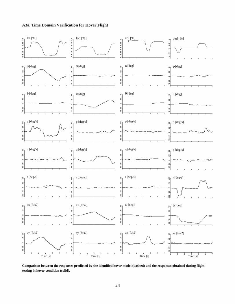
A3a. Time Domain Verification for Hover Flight

Comparison between the responses predicted by the identified hover model (dashed) and the responses obtained during flighttesting in hover condition (solid).

lat [%] lon [%]

θ [deg]

φ [deg]φ [deg]

θ [deg]

col [%]

φ [deg]φ [deg]

θ [deg]θ [deg]

ped [%]

p [deg/s]p [deg/s]

q [deg/s] q [deg/s]

p [deg/s]p [deg/s]

q [deg/s]q [deg/s]

r [deg/s] r [deg/s] r [deg/s] r [deg/s]

ax [ft/s2] ax [ft/s2]

ay [ft/s2] ay [ft/s2]

ψ [deg] ψ [deg]

az [ft/s2] az [ft/s2]

Time [s] Time [s] Time [s] Time [s]

25

A3b. Time Domain Verification for Cruise Flight

Comparison between the responses predicted by the identified cruise model (dashed) and the responses obtained during flighttesting in cruise condition (solid).

lat [%] lon [%]

θ [deg]

φ [deg]φ [deg]

θ [deg]

col [%]

φ [deg]φ [deg]

θ [deg]θ [deg]

ped [%]

p [deg/s]p [deg/s]

q [deg/s] q [deg/s]

p [deg/s]p [deg/s]

q [deg/s]q [deg/s]

r [deg/s] r [deg/s] r [deg/s] r [deg/s]

ax [ft/s2] ax [ft/s2]

ay [ft/s2] az [ft/s2]

ax [ft/s2] vy [ft/s]

az [ft/s2] ay [ft/s2]

Time [s] Time [s] Time [s] Time [s]