Helicopter Dynamic Model Identification using Conditional...

American Institute of Aeronautics and Astronautics

1

Helicopter Dynamic Model Identification using Conditional Attitude Hold Logic

Sunggoo Jung1, David Hyunchul Shim2

Unmanned Systems Research Group, Department of Aerospace Engineering, Korea Advanced Institute of Science and Technology (KAIST), Deajeon, 34141, South Korea

and

Eung-Tai Kim3

Aviation Research Division, Korea Aerospace Research Institute (KARI), Deajeon, 34133, South Korea

A parameter identification method was proposed for flight vehicles with dynamic models that are difficult to identify due to their highly coupled characteristics. The existing off-axis noise input method, which is used for reducing the correlation between the primary and secondary inputs, has a difficult-to-obtain convergence condition under the hold trim state. In addition, the existing method cannot easily identify high frequency dynamics due to the off-axis input noise. On the other hand, the proposed identification method relied on a computer-generated sweep in the frequency-domain, which could produce a more accurate model than the existing perturbation model. Moreover, the proposed conditional attitude hold logic described the actual pilot's motion by activating the controller when the Euler angle measurements exceeded a pre-defined angle. The proposed method was used with the Bo-105 helicopter nonlinear simulation model, and the identified coupled rotor/fuselage nine-degree-of-freedom results were reliable and comparable to those obtained with the existing perturbation model.

Nomenclature

A = stability matrix of the helicopter flight dynamics model B = control matrix of the helicopter flight dynamics model C = observation matrix of the helicopter flighty dynamics model

col = collective stick input

lat = lateral stick input

lon = longitudinal-stick input

1 Graduate Researcher, Dept. of Aerospace Eng., KAIST Institute, KAIST, 291 Daehakro, Yuseonggu, Daejeon, South Korea, AIAA Member. 2 Associate Professor, Dept. of Aerospace Eng., KAIST Institute, KAIST, 291 Daehakro, Yuseonggu, Daejeon, South Korea, AIAA Senior Member 3 Head of aerospace research division, KARI, Gwahakro, Yuseonggu, Deajeon, South Korea, AIAA Senior Member


2

ped = pedal inpuyt

f = rotor flap time constant

col = equivalent time delay of collective input

lat = equivalent time delay of lateral input

lon = equivalent time delay of longitudinal input

ped = equivalent time delay of pedal input

I. Introduction

n the helicopter control system design process, accurate dynamic models can increase the chances of success in controller verification testing such as hardware-in-the-loop simulation.1 Two types of approaches have been used

for acquiring the dynamic model of a helicopter: the physics-based model approach and the flight-test data approach. The physics-based approach predicts the model in advance to set-up the helicopter; however, unlike most fixed-wing aircraft, the highly coupled rotor-body dynamic characteristics and aerodynamic effects of a helicopter make the precise model difficult to predict.2 On the other hand, the flight-test data approach utilizes the actual input/output from the flight-test data. Therefore, the flight-test data approach can isolate uncertainties in the identification process and obtain exact control/stability parameters.

Helicopter dynamics can be modeled by a set of differential equations, and the identification process can then be expressed to estimate the matrix component parameters. Hence, during parameter estimation with flight-test data, the maximum-likelihood (ML) estimation theory and time-domain identification approaches have been utilized.3-4 Estimating the parameters in the time domain is a time-efficient approach. Time-domain identification uses doublet or 3-2-1-1 input as control inputs; thus, the duration of one flight-test cycle is reasonably short. However, bias and noise error problems, which are contained in flight-test data, are difficult to resolve with these methods. Furthermore, in the case of a divergent system, the time-domain indentification method cannot predict any parameters in the matrix of the dynamic model.5

A frequency-domain identification approach could resolve these problems. The time-history data is converted to the frequency domain using a fast Fourier transform (FFT); consequently, the effects of bias and noise can be ignored in the identification process. This explains why the system identification process uses frequency sweep data as a control input rather than a time-efficient doublet or 3-2-1-1 input. Abundant and well distributed frequency components can be obtained by a properly designed frequency sweep. From this, the base conditions for acquiring an exact helicopter system model can be established.

There are two forms of frequency sweep flight tests: the piloted frequency sweep and the computer-generated automated frequency sweep. In helicopter dynamics, the highly coupled rotor/fuselage flapping dynamics, coning/inflow dynamics, and engine dynamics are well beyond the general piloted frequency sweep range. Therefore, a suitably designed automated frequency sweep can serve as an alternative method of identifying these high-bandwidth dynamics. However, once the controller is used to maintain the trim condition during the flight test, a high value of cross-control coherence is obtained between the primary and secondary inputs due to feedback input. This correlation contaminates the pure dynamic response; therefore, accurate dynamic model identification cannot be achieved. To avoid input correlation in the feedback system, Tischler and Marzocca6 added distinct white noise to each off-axis input. This method was shown to be effective in resolving the correlation problem; however, noise impedes the identification of the proper controller gain, which causes the system to converge during the frequency sweep flight test.

This paper illustrates a detailed integrated computer-generated frequency sweep approach based on conditional

I


3

attitude hold logic. This logic was developed to avert the correlation problem and to describe the control motionof an actual pilot by conditionally activating the feedback system. The results show that the inputs can be uncorrelated without requiring noise input. Then, the input be used for identification of the nine-degree-of-freedom (9-DOF) hybrid model, which includes rigid body motion and rotor flapping dynamics.

The target vehicle is the Bo-105 helicopter; however, due to the difficulty of an actual flight test, Bo-105 nonlinear simulation model flight testing was performed. The simulation flight test data at hover are presented in detail, and emphasis is placed on the identification performance of the proposed logic. The Comprehensive Identification from Frequency Responses (CIFER®) software is used as an identification tool,8 and accuracy analysis and verification of the identified results were achieved.

II. Frequency-Domain Identification of the Helicopter Dynamic Model

The frequency-domain identification approach can be used to resolve the bias and noise error problems that may occur in the time domain. In addition, it can be applied to an unstable system, which is difficult to estimate in the time domain.6 Therefore, a transformation process is required to convert from the obtained time-history flight test data to the frequency domain. The input/output frequency response of time-history data can be obtained using the Fourier transform. To apply the Fourier transform theory, the area under the input and output curves of the time-history data must remain bounded (Dirichlet condition):

( ) ( )x t dt and y t dt

(1)

The frequency-response estimate can be obtained as follows:

ˆ ( )ˆ ( )ˆ ( )

m m

m m

x x

x y

G fH f

G f (2)

A frequency-domain identification method is used to find the optimal model parameters, which can best fit the frequency response of the flight data and identified dynamic model. To identify the Bo-105 helicopter model, we used the CIFER® software, which specializes in rotorcraft and aircraft dynamic model identification. The CIFER® software estimates the dynamic model based on the minimization algorithm of the following cost-function:

1

2 2

1

20 ˆ ˆnTFn

g c p cl l

J W W T T W T Tn

(3)

Generally, a cost function of 100J reflects acceptable identification results.

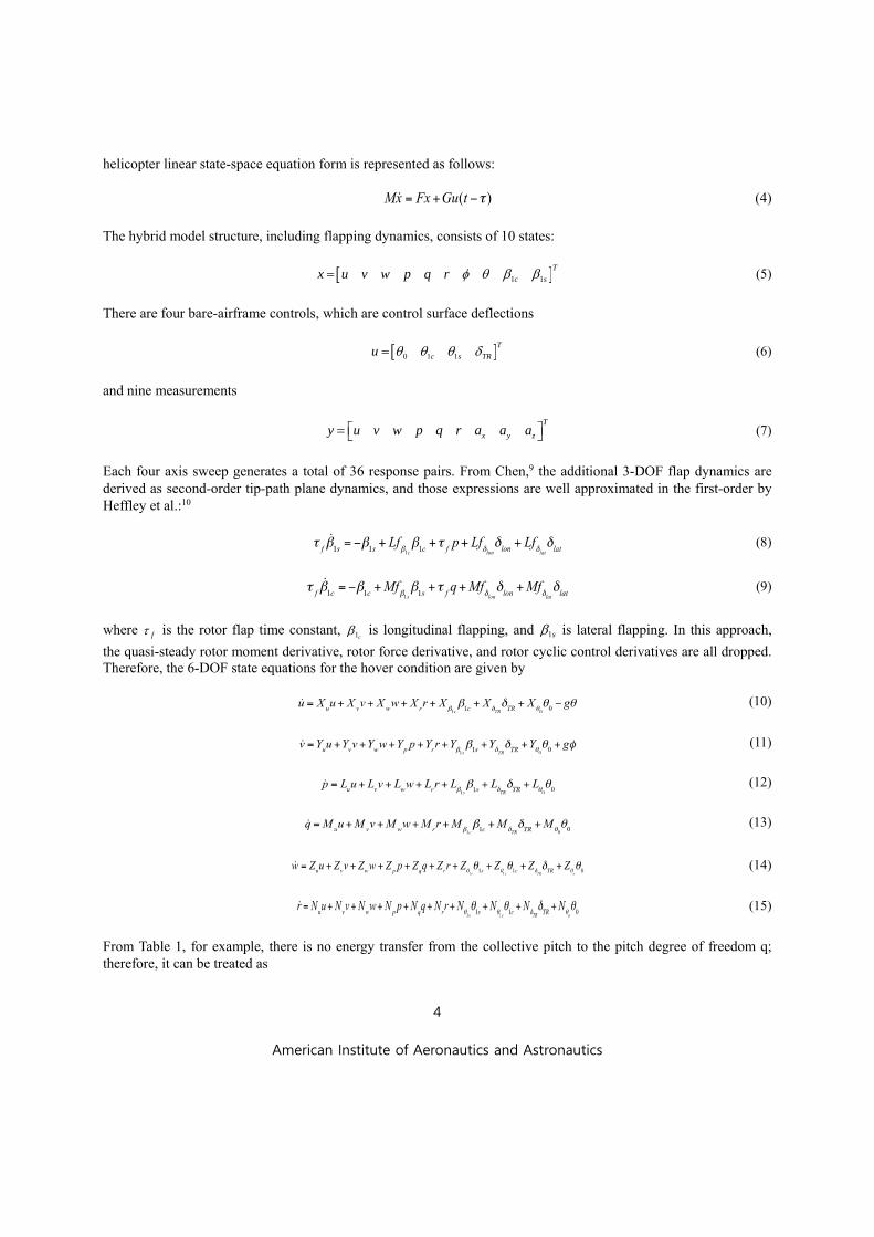
III. Nine-DOF Hybrid Model Identification

Generally, in a fixed wing aircraft, decoupled dynamics occur in the low-to-mid frequencies usually up to 12 rad/s, which can be identified using the 6-DOF quasi-steady identification method. However, in the rotorcraft case, which has highly coupled rotor/fuselage dynamic characteristics such as the Bo-105 helicopter, the frequency ranges are expended up to 31 rad/s (=5 Hz) to include the rotor-flapping dynamics. Therefore, the conventional 6-DOF model identification approach is not suitable, and the 9-DOF hybrid model identification method is more appropriate. The


4

helicopter linear state-space equation form is represented as follows:

(4)

The hybrid model structure, including flapping dynamics, consists of 10 states:

1 1

T

c sx u v w p q r (5)

There are four bare-airframe controls, which are control surface deflections

0 1 1

T

c s TRu (6)

and nine measurements

T

x y zy u v w p q r a a a (7)

Each four axis sweep generates a total of 36 response pairs. From Chen,9 the additional 3-DOF flap dynamics are derived as second-order tip-path plane dynamics, and those expressions are well approximated in the first-order by Heffley et al.:10

(8)

(9)

where f is the rotor flap time constant, 1c is longitudinal flapping, and 1s is lateral flapping. In this approach,

the quasi-steady rotor moment derivative, rotor force derivative, and rotor cyclic control derivatives are all dropped. Therefore, the 6-DOF state equations for the hover condition are given by

(10)

(11)

(12)

(13)

(14)

(15)

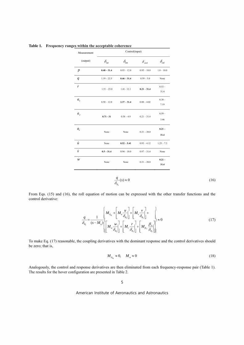
From Table 1, for example, there is no energy transfer from the collective pitch to the pitch degree of freedom q; therefore, it can be treated as


5

Table 1. Frequency ranges within the acceptable coherence

Measurement

(output)

Control(input)

lat lon ped col

p 0.48 – 31.4 0.93 – 12.0 0.95 – 10.0 1.0 – 10.0

q 1.19 – 22.5 0.46 – 31.4 0.59 – 5.0 None

r 1.51 – 23.0 1.41– 12.1 0.21 – 31.4

0.53 –

31.4

xa 0.50 – 12.0 2.37 – 31.4 0.88 – 4.02

0.38 –

7.19

ya 0.71 - 31 0.58 – 4.9 0.21 – 31.4

0.59 –

3.46

za None None 0.21 – 20.0

0.21 –

31.4

u None 0.52 – 5.41 0.93 – 4.12 1.25 – 7.3

v 0.5 – 31.4 0.94 – 10.0 0.97 – 31.4 None

w None None 0.21 – 20.0

0.21 –

31.4

0

( ) 0q

s

(16)

From Eqs. (15) and (16), the roll equation of motion can be expressed with the other transfer functions and the control derivative:

0

0 0

0

1

0 0 0

1

10

( )

c

u v

qc

w r

u vM M M

q

s M w rM M M

(17)

To make Eq. (17) reasonable, the coupling derivatives with the dominant response and the control derivatives should be zero; that is,

00, 0wM M

(18)

Analogously, the control and response derivatives are then eliminated from each frequency-response pair (Table 1). The results for the hover configuration are presented in Table 2.


6

Table 2. The 9-DOF identification model structure (Bo-105 simulation, hover)

M Matrix Structure G Matrix Structure

1 1

1

1

1.00 0 0 0 0 0 0 0 0 0

0 1.00 0 0 0 0 0 0 0 0

0 0 1.00 0 0 0 0 0 0 0

0 0 0 1.00 0 0 0 0 0 0

0 0 0 0 1.00 0 0 0 0 0

0 0 0 0 0 1.00 0 0 0 0

0 0 0 0 0 0 1.00 0 0 0

0 0 0 0 0 0 0 1.00 0 0

0 0 0 0 0 0 0 0 * 0

0 0 0 0 0 0 0 0 0

c s

c f

s f

u v w p q r

u

v

w

p

q

r

0 1 1

1

1

* 0 0 *

* 0 0 *

*

* 0 0 *

0 0 *

* * * *

0 0 0 0

0 0 0 0

0 * 1 0

0 1 * 0lat

lon

c s TR

c c b

c

c

s

u XDC XDP

v YDC YDP

w ZDC ZDL ZDLo ZDP

p LDC LDP

q MDC MDP

r NDC NDL NDLo NDP

Mf

Lf

F Matrix Structure Tau Matrix Structure

1

1

1

1

11

1 1

1

* 0 0 * 0 * 0

* * * 0 * 0 0

* * 0 0 0 0

* * 0 * 0 0 0 *

* 0 0 * 0 0 * 0

* * * * 0 0 0 0

0 0 0 1 0 0 0 0 0 0

0 0 0 0 1 0 0 0 0 0

0 0 0 0 0 0 0 1 *

c

s

s

c

s

c sa b

u v w r

bu v w p r

c c c cu v w p q r

a bu v w p r

a bu v w r

a bu v w p q r

c f

u v w p q r

u X X X X g X

v Y Y Y Y Y g Y

w Z Z Z Z Z Z

p L L L L L L

q M M M M M

r N N N N N N

Mf

11 0 0 0 0 0 0 0 * 1cs f Lf

0 1 1

0 1 1

0 1 1

0 1 1

0 1 1

0 1 1

0 1 1

0 1 1

0 1 1

0 1 1

* * * *c s T R

c s T R

c s T R

c s T R

c s T R

c s T R

c s T R

x c s T R

y c s T R

z c s T R

u

v

w

p

q

r

a

a

a

*Indicates a free derivative a

Fixed parameter to trim calculation value. b

Dropped parameter from 6-DOF identification c

Eliminated from model structure.

IV. Control Input Design

There are several types of inputs used for identifying the dynamic model such as steps, doublets, 3-2-1-1 (multi-steps), and frequency sweep. Among these, frequency sweep input shows the most even spectrum distribution in the frequency domain. Therefore, the frequency sweep input was selected as an optimal input for identifying the system dynamics based on the frequency domain. The frequency sweep input method obtained the vehicle frequency response by sweeping the control stick of the vehicle in the frequency range of interest. However, high frequency dynamics, especially those beyond 3 Hz, were difficult to identify due to the limitation of the piloted input speed. Hence, for performing a high-speed sweep, the computer-generated frequency sweep method could be used.


7

A. Computer-generated frequency sweep

Tischler11 developed a computer-generated frequency sweep signal with an exponentially increasing sweep form. The exponential form was applied to spend more time in the low-frequency range than the high-frequency range to achieve an even spectral energy:

1( / )

min 2 max min0sin 1

recrec

T C t Tsweep A C e dt (19)

where A is the sweep amplitude and recT is flight test or simulation record time. The maximum input frequency max and minimum frequency min were selected as 31.4 rad/s and 0.3 rad/s, respectively, to identify the high frequency rotor-flapping dynamics. The frequency sweep record length was set to

90recT (20)

which is from1

max(4 5)recT to T (21)

max

min

2T

(22)

Thus, the sweep parameters in Eq. (19) are given as follows:

min max90, 0.05, 0.3 / , 31.4 / ( 5 )recT A rad s rad s Hz (23)

The resultant frequency sweep input using Eqs. (19) and (23) is shown in Fig. 1.

Figure 1. Automated frequency sweep input form

Figure 2. Feedback system to maintain trim condition during flight test

0 10 20 30 40 50 60 70 80 90-5

-4

-3

-2

-1

0

1

2

3

4

5

time(sec)

stick input (%

)


8

B. Conditional Attitude Hold Logic

Maintaining the trim state of an unstable system during the sweep test is not easily achieved without a stability augmentation system (SAS) or controller (Fig. 2). When the controller acts, the feedback loop of controller causes correlation between the primary and secondary input.

For example, when the correlation exists between lateral and longitudinal inputs 0lat lon

G , the roll rate frequency

response of the lateral input will be

2

1 /

1

lat lat lon lon lon lon lat

lat lat lat lon

p p p

lat

G G G G Gp

G

(24)

The correlation terms contaminate the single-input single-output (SISO) solution, and accurate identification cannot be achieved. Hence, correlation between the inputs should be avoided. Tischler11 set guidelines of acceptable cross-control coherence as

1 2

2 0.5ave (25)

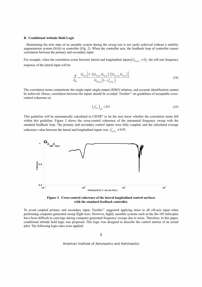
This guideline will be automatically calculated in CIFER® to let the user know whether the correlation terms fall within this guideline. Figure 3 shows the cross-control coherence of the automated frequency sweep with the standard feedback loop. The primary and secondary control inputs were fully coupled, and the calculated average

coherence value between the lateral and longitudinal inputs was 2 0.95lon lat .

Figure 3. Cross-control coherence of the lateral longitudinal control surfaces with the standard feedback controller.

To avoid coupled primary and secondary input, Tischler11 suggested applying noise to all off-axis input when performing computer-generated sweep flight tests. However, highly unstable systems such as the Bo-105 helicopter have been difficult to converge during computer-generated frequency sweeps due to noise. Therefore, in this paper, conditional attitude hold logic was proposed. This logic was designed to describe the control motion of an actual pilot. The following logic rules were applied:

10-1

100

101

102

0.2

0.6

1 G

lat

lon

FREQUENCY (RAD/SEC)

Coh

eren

ce


9

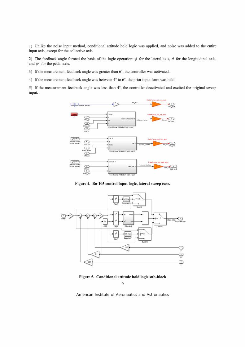
1) Unlike the noise input method, conditional attitude hold logic was applied, and noise was added to the entire input axis, except for the collective axis.

2) The feedback angle formed the basis of the logic operation: for the lateral axis, for the longitudinal axis, and for the pedal axis.

3) If the measurement feedback angle was greater than 6°, the controller was activated.

4) If the measurement feedback angle was between 4° to 6°, the prior input form was held.

5) If the measurement feedback angle was less than 4°, the controller deactivated and excited the original sweep input.

Figure 4. Bo-105 control input logic, lateral sweep case.

Figure 5. Conditional attitude hold logic sub-block


10

Figure 4 represents the simulation control input logic based on the above rules, and Fig. 5 shows the inner logic of the conditional attitude hold block. This conditional attitude hold block was included with all control input except for the collective axis, and white noise was applied to the off-axis input as discussed above. Simulated lateral frequency sweep input data are represented in Fig. 6, which shows a gradual increase in the frequency throughout the sweep. Springs were also observed, especially in low frequencies, which seemed to be an effect of the activated conditional attitude hold logic when the feedback angle exceeds the reference angle. Figure 7 shows the cross-control coherence of the automated frequency sweep with conditional attitude hold logic. Much lower cross-control coherences were observed compared to those obtained with the standard controller (Fig. 3), and the calculated average coherence value between the lateral and longitudinal input was 2 0.17

lon lat .

V. Results and Verification

Forty-one parameters must be identified for the Bo-105 helicopter dynamics. Each identified parameter had a minimum value of the cost-function given in Eq. (3). In each axis, two flight simulations were performed to obtain acceptable flight data within the frequency range of interest. Figure 8 and Fig. 9 show the frequency sweep input in lateral case. The two flight data sets were merged into one consecutive time history. Therefore, a total of 180 s of time-history data was used in identification process, and the frequency range of interest was 0.01 rad/s to 31.4 rad/s.

Figure 6. Input time histories of the lateral frequency sweep input based on the conditional attitude hold logic.


11

Figure 7. Cross-control coherence of the lateral longitudinal control surfaces based on the conditional attitude hold logic.

Figure 8, Input case 1: 0.2 rad/s to 31.4 rad/s.

Figure 9. Input case 2: 0.01 rad/s to 18.85 rad/s.

10-1

100

101

102

0.2

0.6

1

G

lat

lon

FREQUENCY (RAD/SEC)

Co

her

ence


12

The initial values of the 9-DOF parameters were obtained from the 6-DOF identification results.11 In the 6-DOF identification process, the rolling moment derivative pL and pitching moment derivative qM were identified. From

those identification values, the initial values of 1s

L and 1c

M were calculated as

1sp feffectiveL L (26)

1cq feffectiveM M (27)

Table 3 shows the identified 9-DOF hybrid model parameters with the Cramer-Rao (CR) bounds and insensitivity accuracy analysis. With the exception of

1cfL

, none of the identified parameters had an insensitivity over 10% or

CR bound exceeding 20%, which were the bounds for reasonable accuracy. However, when 1cfL

was removed from

the analysis, the average cost-function considerably increased; therefore, 1cfL

was retained.

Speed stability derivatives such as , ,v uL M and vN were calculated from trim data; therefore, those values were fixed

in the identification process. The equations relating the speed stability derivatives and trim data are12-14

lon

lon uu w

w

ZM M M

u Z

(28)

lat ped

pedlatvL L L

v v

(29)

ped

pedvN N

v

(30)

The results are presented in Eq. (31), and the detailed values are given in Table 3.

0.7149

0.04081

0.07651

v

v

u

L

N

M

(31)


13

Table 3. Identified parameters for the 9-DOF Bo-105 simulation model. a

Engineering

Symbols

Value

(9-DOF)

CR

%

Insensitivity

%

Engineering

Symbols

Value

(9-DOF)

CR

%

Insensitivity

%

f 0.06416 3.537 0.4173 Zw -0.3131 6.5240 2.7400

Xu c-0.0103 -------- --------

Zq b 0.000 ---------- ----------

Xv b 0.000 Zr 0.5863 4.2180 1.3390

Xw 0.0506 6.9670 2.9730 Lr 0.1463 17.1900 7.3970

Xr -0.0788 8.0500 3.2070 1L s -173.4000 4.0020 0.7572

1X c 12.6400 3.5060 0.8290 N r -0.5777 4.4050 1.5630

Yu b 0.000 ---------- ---------- 0Z -120.600 2.6930 1.1520

Yv -0.0281 9.7400 3.4270 1Z c b 0.000 -------- --------

Yw b 0.000 ---------- ---------- 1Z s b 0.000 -------- --------

Yp 0.3052 5.6550 2.2450 Mf lat 0.1922 4.3460 1.0960

Yr 0.1456 5.4550 1.9390 Mf lon -0.8346 4.0440 0.9512

1Y s d -12.6400 ---------- ---------- Nf lat 0.8144 4.0840 0.5867

Zu b 0.000 ---------- ---------- Nf lon 0.2890 4.8570 0.6677

Zv 0.000 ---------- ----------

a All results in SI units b Eliminated from the model structure c Fixed parameters from the trim data d Constrained parameter in the model structure

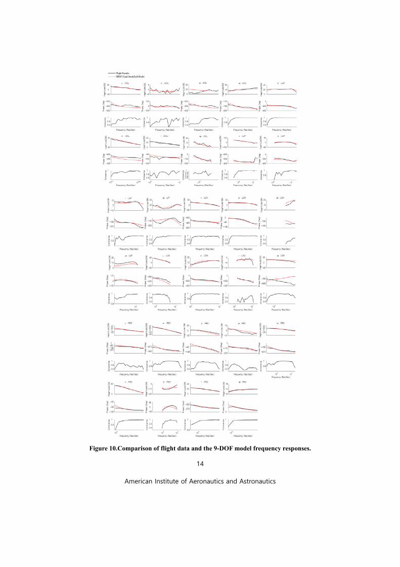
The frequency-domain comparison between the identification data and simulation results in the hovering condition is presented in Fig. 10 Good agreement was observed between the two results, and especially good agreement was observed in the angular rate responses, which is important in control system design.


14

Figure 10. Comparison of flight data and the 9-DOF model frequency responses.


15

VI. Conclusion

A 9-DOF dynamic model for the Bo-105 nonlinear simulation model helicopter has been developed using the frequency-domain identification method. Conditional attitude hold logic was proposed that successfully resolved the correlation problem between the primary and secondary input. The existing noise input method needed a complex gain tuning process for the controller in order to prevent system divergence during the frequency sweep test; however, by using the proposed logic, the system stable was shown to be stable without requiring a complex process. Hence, the total flight test time for model identification could be effectively reduced. The model captured a frequency range up to 30 rad/s, which was in the frequency range of rotor dynamics. The proposed logic will be tested in the future by a TREX 700L unmanned helicopter for real-world validation.

Acknowledge

This research was part of the project “Development of a core technology and infra technology for the operation of USV with high reliability” funded by the Ministry of Oceans and Fisheries, Korea

s

References 1Soderstorm, T. and Stoica, P., System Identification, Prentice-Hall International, 1989.

2Hamel, P. G. and Kaletka, J., “Advances in Rotorcraft System Identification,” Progress in Aerospace Sciences, Vol. 33, No. 3-4, March-April 1997, pp. 259-284.

3Milne, G. W., MMLE3 Identification Toolbox for State-Space Identification using MATLAB, Control Models (2000).

4Jategaonkar, R. and Thielecke, F., “ESTIMA an integrated software tool for nonlinear parameter estimation,” Aerospace Science and Technology, Vol. 6, No. 8, December 2002, pp. 565-578.

5Bendat, J. S. and Piersol, A. G., Engineering Applications of Correlation and Spectral Analysis, 2nd ed., Wiley Interscience, 1993.

6Tischler, M. B. and Marzocca, P., “Adaptive and Robust Aeroelastic Control of Nonlinear Lifting Surfaces with Single/Multiple Control Surfaces: A Review,” International Journal of Aeronautical and Space Sciences, Vol. 11, No. 4, December 2010, pp. 285-302.

7Seher-Weiß, S., “User’s Guide FITLAB Parameter Estimation Using MATLAB,” DLR Institute of Flight Systems, Vol. 111, 2007.

8CIFER User's Guide, Version 6.1.00, University Affiliated Research Center, Moffett Field, CA.

9Tischler, M. B. and Remple, R. K., Aircraft and Rotorcraft System Identification - Engineering Methods with Flight Test Examples, 2nd ed., AIAA Education Series, 2012.

10Curtiss, Jr., H. C., “Dynamic stability of V/STOL aircraft at low speeds.” Journal of Aircraft, Vol. 7, No. 1, January-February 1970, pp. 72-78.

11Padfield, G. D. Helicopter flight dynamics, John Wiley & Sons, 2008.

12Cooke, A. K. and Fitzpatrick, E. W. H., Helicopter Test and Evaluation, AIAA Educational Series, AIAA, Reston, VA, 2002, pp. 185-194.

Helicopter Dynamic Model Identification using Conditional...

Documents

Transcript of Helicopter Dynamic Model Identification using Conditional...