Seasonal Adjustment of NIPA data

Jonathan H. Wright*

July 29, 2018

Abstract

In the 2018 comprehensive update of the national income and product accounts, the Bu-reau of Economic Analysis released not seasonally adjusted data, and modified its seasonaladjustment procedures. I find some indication of residual seasonality in the seasonally ad-justed data as published before this update. The evidence for residual seasonality is weakerin the seasonally adjusted data after the update. I also directly seasonally adjusted the ag-gregate not seasonally adjusted data, and this entirely avoids residual seasonality. The aver-age absolute difference between my seasonally adjusted real GDP data and the current of-ficial published version is 1.1 percentage points in quarter-over-quarter annualized growthrates.

*Department of Economics, Johns Hopkins University, 3400 North Charles St., Baltimore MD 21218. Email:wrightj@jhu.edu

1 Introduction

In the 2018 comprehensive update of the national income and product account (NIPA) data,

the Bureau of Economic Analysis (BEA) made changes to the method for seasonal adjustment

and began publishing quarterly not seasonally adjusted (NSA) data, both current and chained

dollar, for GDP and its major components going back to 2002.1 This is part of an overhaul of

seasonal adjustment procedures being undertaken by BEA, as discussed in McCulla and Smith

(2015) and Moulton and Cowan (2016). These are very welcome developments. In particular,

the publication of NSA data is an enormous advance in transparency. Data users will naturally

question how the BEA and the agencies that provide data to the BEA undertake seasonal ad-

justment. These users will now be able to seasonally adjust the data themselves, at least at the

level of aggregation at which the data are published. NIPA data are one of the great advances

in economic analysis of the 20th century2, and macroeconomic data generally exhibit seasonal

fluctuations of comparable amplitude to the business cycle. This makes it very valuable for

economists to have the source data necessary for studying the seasonal patterns in NIPA data.3

Moreover, the unadjusted data may be useful sources of identification in macroeconomic mod-

els (Ghysels, 1988; Barsky and Miron, 1989; Hansen and Sargent, 1993; Sims, 1993; Saijo, 2013).

The practice of statistical agencies releasing only seasonally adjusted data has been criticized

by a number of authors including Maravall (1995) and Wright (2013).

Unlike many other economic statistics, seasonal adjustment of the NIPA data is not all con-

ducted by one agency. Although BEA compiles the NIPA data, many of the data come in the

door of BEA already seasonally adjusted by other agencies, such as the Census Bureau. To com-

pile the NSA data, BEA had to go back to those other agencies to request unadjusted data. The

1BEA had in the past published current dollar NSA data, but ceased doing so in 2008 as a cost cutting measure.The new data consist of nominal, real and price series for GDP and its major components. I do not attempt to usethe old data, because my focus in this paper is on real data and to some extent on price indices.

2See Landefeld, Seskin, and Fraumeni (2008) for a discussion of NIPA history and methods.3Until now, researchers worried about the adequacy of seasonal adjustment have been forced to undertake a

double seasonal adjustment—seasonally adjusting the seasonally adjusted data (Rudebusch, Wilson, and Mahedy,2015; Boldin and Wright, 2016; Phillips and Wang, 2016). But working with the NSA data is clearly better.

1

process of compiling NSA data was therefore much more cumbersome than one might initially

suppose. Also, the decentralized nature of NIPA seasonal adjustment means that it is not doc-

umented or replicable by outside researchers in the same way as seasonal adjustment in other

macroeconomic data, such as the BLS establishment survey.

Figure 1 plots the level of topline real GDP data without seasonal adjustment. A sawtooth sea-

sonal pattern can clearly be seen where the level of GDP typically drops about 3 percentage

points (not at an annualized rate) in the first quarter, and rebounds in the rest of the year. Thus,

in the raw data, there is a drop in output of comparable magnitude to a recession every winter.

In this note, I compare three different sets of NIPA numbers. The first are the data as seasonally

adjusted by BEA just before the recent update. The second are the data as seasonally adjusted by

BEA after the update. Of course, the change in seasonal adjustment methodology was just a part

of the 2018 benchmark revision. In the third dataset, I take the NSA data as now published by

the BEA and seasonally adjust them using TRAMO-SEATS, which is based on a seasonal ARIMA

model, as opposed to the moving average filters that are the mainstay of seasonal adjustment

in North America.4 This approach differs from that used in official NIPA seasonal adjustment

in a number of ways. Notably, the official seasonal adjustment is done at the disaggregate level

(the indirect approach), whereas I instead do the seasonal adjustment at the aggregate level (the

direct approach). The indirect approach has the advantage that the aggregate data are exactly

the sum of the disaggregate components. This is lost with the direct approach.5 On the other

hand, seasonal adjustment at the disaggregate level might be more prone to leaving residual

seasonality in aggregate data. This can arise from sources including:

1. Some of the components are not seasonally adjusted at all on the grounds that the sea-

sonality in those components is not sufficiently pronounced. There may be many com-

ponents that each exhibit minor seasonality where that seasonality is however positively

correlated across the components. The omitted seasonality may therefore be quite con-

4See Wright (2017) for arguments for using an ARIMA-based parametric approach to seasonal adjustment.5It is lost in any case when using chained dollar data.

2

sequential in the aggregate, even if it was not at the component level.

2. Monthly series may be deemed to have no seasonality and are consequently not season-

ally adjusted at all, but there may be a material seasonal pattern after aggregation to the

quarterly frequency (Moulton and Cowan, 2016).

3. Revision policies preventing seasonal adjustments being applied to historical data. The

latest benchmark revision has softened, but not eliminated, these revision policies.

4. BEA intentionally avoids seasonally adjusting series related to government policy even

where seasonal effects are believed to be present, to make the effects of policy more trans-

parent (Moulton and Cowan, 2016).

The possibility of residual seasonality being created from an interaction of pre-testing with ag-

gregation is heightened by the Census Bureau guideline that a series should not be seasonally

adjusted unless the F-statistic for seasonality exceeds 7 (McDonald-Johnson, Monsell, Fescina,

Feldpausch, Hood, and Wroblewski, 2010).6

In my implementation of TRAMO-SEATS, I use the automatic ARIMA model selection method

of Gómez and Maravall (1996, 2013). I incorporate Easter and trading day effects within the

TRAMO-SEATS program, and use all the available NSA data back to 2002 for the seasonal ad-

justment. Modeling choices in seasonal adjustment are of course very consequential, but this

seems to be a reasonable benchmark.

The plan for the remainder of this paper is as follows. In section 2, I report the alternative

seasonally adjusted series. In section 3, I test for residual seasonality in these series. Section 4

concludes.6See Maravall (2006) and Chapter 8 of Bloem, Dippelsman, and Mæhle (2001) for more discussion of the direct

and indirect approaches.

3

2 Alternative series

The series that I consider in this paper are as follows: GDP, personal consumption expenditures,

nondurable goods, durable goods, services, gross private domestic investment, equipment,

structures intellectual property investment, residential investment, exports, imports, govern-

ment spending, federal defense and non-defense spending and state and local government

spending, all in chained dollars, as well as the GDP, personal consumption expenditures (PCE)

and core PCE price indices. The internet appendix to this paper gives the levels of all of these 19

series with all of the approaches to seasonal adjustment.7 The NSA data does not include core

PCE, and so this is excluded from the directly seasonally adjusted series.

The average absolute difference between the current official data on real GDP quarter-over-

quarter growth rates and my direct seasonal adjustment is 1.1 percentage points at an annu-

alized rate. Table 1 reports growth rates for real GDP back to 2014 using the three approaches

to seasonal adjustment. In 2018, real GDP growth rates in the first two quarters are 3.1 and 4.0

percentage points respectively, as opposed to 2.2 and 4.1 percentage points in the published

data.

Table 2 reports the average growth rates since 2002Q1 in each of the four quarters for all of these

series and with all of the approaches to seasonal adjustment. Here and throughout, I use the

post-2002 sample period to accord with the availability of NSA data.

Apparent seasonal patterns can be seen in many of the seasonally adjusted series as published

before the 2018 benchmark revision. For example, the average growth rate of real GDP in the

first quarter was 1.1 percentage points, more than one percentage point lower than the aver-

age for the other quarters of the year. Particular first-quarter weakness can be seen in federal

defense spending. This pattern of weakness in first quarter GDP growth and some of its com-

7The first two methods of course involve no seasonal adjustment on my part; they are just reporting the data aspublished by the BEA.

4

ponents was noticed by Wall Street economists and the press8, and has been written about

extensively (Stark, 2015; Rudebusch, Wilson, and Mahedy, 2015; Gilbert, Morin, Paciorek, and

Sahm, 2015; Groen and Russo, 2015; Phillips and Wang, 2016; Lunsford, 2017). The finding of a

particularly strong negative first quarter effect in federal defense spending is a common theme

of much of this existing work. There is also some sign of residual seasonality in price indices,

with core PCE inflation running a little higher in the first half of the year than the second half of

the year, as found earlier by Peneva (2014).

There is less sign of residual seasonality in the data as published in the 2018 benchmark re-

vision. The average growth rate in the first quarter was revised up to 1.5 percentage points,

closer to but still lower than the average for the other quarters of the year. The first quarter

effect in federal defense spending has disappeared. Meanwhile, there is no sign of residual sea-

sonality in the directly seasonally adjusted data. Although first quarter real GDP growth is on

average higher with the TRAMO-SEATS directly seasonally adjusted data than in the published

numbers, in individual years the first quarter reading using the direct seasonal adjustment is

sometimes higher and sometimes lower.

Table 2 reports some summary statistics for the growth rate series with the three different ap-

proaches to seasonal adjustment. The summary statistics are the sample standard deviation

abd the first and fourth sample autocorrelations. These summary statistics are mostly simi-

lar before and after the benchmark revision, but the benchmark revision generally slightly re-

duced the fourth autocorrelation, consistent with better seasonal adjustment. Comparing the

post-revision published data with the directly seasonally adjusted data, the directly seasonally

adjusted data are typically more persistent in the sense that the first autocorrelation is higher.

This is particularly true for consumption (where the coefficient goes from 0.51 in the published

data to 0.86 in the directly adjusted data) and durables (where the coefficient goes from 0.14 to

8Alec Phillips of Goldman Sachs was one of the first to highlight the phenomenon. See also a CNBC article bySteve Liesman https://www.cnbc.com/2015/04/21/the-mysterious-case-of-weak-1q-gdp-for-30-years.html.

5

0.50). This suggests that the directly seasonally adjusted data might be easier to forecast.9

3 Testing for statistical significance

The seasonal adjustment approach is clearly important. The low level of average real GDP

growth in the first quarter raises a suspicion of residual seasonality in the pre-benchmark re-

vision official data and still, to a lesser extent, in the post-benchmark revision data. But it is

useful to have a formal test for remaining seasonal patterns in the seasonally adjusted data. I

take an approach following Canova and Hansen (1995). Let yt be any seasonally adjusted series,

and let D j t be a dummy that is 1 if quarter t is in the j th quarter of the year and 0 otherwise.

Consider the regression:

yt =α+ρyt−1 +β1D1t +β2D2t +β3D3t +εt . (3.1)

Consider a Wald test of the hypothesis that β1 =β2 =β3 = 0. In this Wald test, I use Newey-West

standard errors, while the inclusion of a lag in equation (3.1) serves as a form of pre-whitening.

This approach to testing for residual seasonality differs from the F-test in the X-13 seasonal

adjustment process in that a lagged dependent variable is included and heteroskedasticity and

autocorrelation robust standard errors are used, whereas the X-13 uses the ordinary F-statistic

with a critical value of 7 as a more informal adjustment for omitted heteroskedasticity and serial

correlation (McDonald-Johnson, Monsell, Fescina, Feldpausch, Hood, and Wroblewski, 2010).

Following the advice of Lazarus, Lewis, Stock, and Watson (forthcoming), the lag truncation

parameter is set to 1.3T 1/2 (rounded to the nearest integer) where T is the sample size and the

non-standard “fixed b" critical values of Kiefer and Vogelsang (2005) are used.

Table 4 reports the Wald test p-values for each series and each method of seasonal adjustment,

9This is purely speculative—these TRAMO-SEATS seasonally adjusted data use a two-sided filter and were notavailable in real time.

6

over the post-2002 sample. In the series as published by BEA before the benchmark revision,

there is significant residual seasonality at the 5 percent level in structures and federal defense

spending alone. The p-value for real GDP is 0.18.

Thus, although the residual seasonality in the pre-revision data appears economically signif-

icant, it is typically not statistically significant at conventional levels, with some exceptions.

Existing work has generated mixed conclusions regarding the statistical significance of residual

seasonality, with results sensitive to the precise testing methodology and sample period. Stark

(2015), Rudebusch, Wilson, and Mahedy (2015) and Lunsford (2017) conclude that there is im-

portant residual seasonality, while Gilbert, Morin, Paciorek, and Sahm (2015) and Groen and

Russo (2015) are more skeptical.

Where we fail to reject the null hypothesis of no residual seasonality, it is possible that the ap-

parent residual seasonality is a “fluke”, caused for example by unusual weather. Temperatures

in the first quarter have been below their 30-year historic average in the first quarter for 13 out

of the last 17 years, using the updated dataset of Boldin and Wright (2016).10 But it is also pos-

sible than the residual seasonality is real, but the power of the test is insufficient to detect it. To

illustrate this I did a small Monte-Carlo simulation. The design is:

yt = zt + st (3.2)

where

zt = 0.4zt−1 +εt , (3.3)

εt is iidN(0,5) and

st =−θ, t = 1,5,9, .. (3.4)

st = θ

3, t 6= 1,5,9, ..

10However, federal defense spending might seem an unlikely component to be heavily influenced by unusuallycold winters.

7

The innovation variance and persistence are designed to be representative of post Great Mod-

eration real GDP growth data, in annualized quarter-over-quarter percentage changes, while st

represents a simple form of omitted deterministic seasonality. The parameter θ can be thought

of as representing the magnitude of a potential negative first quarter effect.

I simulated the power of the Wald test based on equation (3.1) when applied to these data with

varying values of θ and a sample size of T = 64, corresponding to 16 years of data. The power

curve for a 5 percent nominal test size is plotted in Figure 2. A value of θ of 1, corresponding to

quarter-over-quarter growth in one quarter being lower than the year-average by 1 percentage

point at an annualized rate has a probability of being detected of a bit less than 40 percent.

Thus a degree of residual seasonality that seems economically quite significant might fail to be

detected. Estimation and hypothesis testing are quite distinct problems, and from a decision

theoretic perspective, the fact that a parameter is not statistically significantly different from

zero should not lead one to view zero as the best guess for that parameter, especially when the

power of the test is low. In the same way, I think that it is unwise to walk away from the apparent

residual seasonality in pre-revision data even in cases where it is not statistically significant

at conventional significance levels. This is especially true since the power of the test is low,

and there is reason to expect at least some residual seasonality given the construction of the

published seasonally adjusted numbers, as discussed in the introduction. The point estimate

indicates that there was material residual seasonality in the BEA data as published before the

benchmark revision, although the magnitude of that residual seasonality is hard to determine

with much precision.

In the post-revision data (second column of Table 4), residual seasonality is still statistically

significant at the 5 percent level for structures and is now statistically significant for equipment.

The p-value for topline GDP is 0.66, and the residual seasonality is not significant for federal

defense.

In the directly seasonally adjusted data (last column of Table 4), residual seasonality is statis-

8

tically insignificant at the 10 percent level in every case. In fact the p-values are mostly close

to 1, indicating that the Wald statistic is typically in the left tail of the asymptotic distribution,

but this makes sense because the series being tested were directly constructed to purge any

seasonal pattern.

3.1 Time-varying residual seasonality

Existing evidence (e.g. Moulton and Cowan (2016)) indicates that the potential seasonal pat-

terns in seasonally adjusted data are somewhat sensitive to the sample period. To some extent,

this is not surprising. For one thing, in 2015 the BEA revised its seasonal adjustment proce-

dures but applied the modified procedures only to data starting in 2012 (McCulla and Smith,

2015). After the 2018 benchmark revision, revisions to seasonal adjustment were extended fur-

ther back in time, but with time spans that vary by component. All this means that there has to

be at least some instability in seasonal patterns in the published seasonally adjusted data, both

before and after the 2018 benchmark revision.

One can formally test for the stability of seasonal patterns using the approach of Canova and

Hansen (1995) who apply the test of Nyblom (1989) to assess the stability of the β coefficients

in equation (3.1). The test statistic is:

L = 1

T 2ΣT

t=1Σti=1z ′

i Ω−1Σt

i=1z ′i (3.5)

where zi = (D1i ei ,D2i ei ,D3i ei )′, ei is the residual from equation (3.1), Ω= Γ(0)+ΣMj=1

M+1− jM+1 (Γ( j )+

Γ( j )′) and Γ( j ) = T −1ΣT− jt=1 zt z ′

t+ j . I report the p-values in Table 5, over the period 2002Q1-

2018Q1 using the three seasonally adjusted series. However, as before, in the Newey-West esti-

mate of the variance-covariance matrix, I set the lag truncation parameter M to 1.3T 1/2, and use

nonstandard “fixed b" critical values. Cho and Vogelsang (2017) derive the limiting distribution

of the sup-F structural stability test using “fixed-b" asymptotics and by the same arguments

9

under standard assumptions:

L → L∗ ≡∫ 1

0B(r )′Ω−1B(r )dr (3.6)

where

Ω= 2

b

∫ 1

0B(s)B(s)′d s − 1

b

∫ 1−b

0[B(s)B(s +b)′+ B(s)B(s +b)]′d s

B(r ) = B(r )− r B(1), B(r ) is a Brownian motion (3x1 in this case) and b = limT→∞ M/T . This is

the distribution that is used to provide the p-values in Table 5.

In the series as published by BEA before the benchmark revision, there is significant time-

variation in the residual seasonality at the 5 percent level in consumption, durables and federal

defense spending, and at the 10 percent level in the GDP price index. Rejection of the hypothe-

sis of constant seasonality implies residual seasonality in at least some part of the sample. After

the benchmark revision, it is significant at the 5 percent level only for durables, and at the 10

percent level for consumption. With directly seasonally adjusted data, it is significant only for

the PCE price index.

3.2 Joint testing for stable and zero residual seasonality

If the seasonal adjustment procedure works as one would hope, the coefficients β1, β2 and β3

should be both constant and equal to zero, when applied to seasonally adjusted data. The Wald

test (Table 4) tested that they were zero and the stability test (Table 5) tested that they were

constant. To test the joint hypothesis, I consider the sum of the stability test and the Wald test,

L+W , where W denotes the Wald test statistic in equation (3.1). The asymptotic distribution of

this joint test statistic is:

L∗+B(1)′Ω−1B(1) (3.7)

Table 6 shows the p-values from comparing the joint test with this asymptotic distribution over

10

the period 2002Q1-2018Q1, again using the three seasonally adjusted series. The idea of this test

is similar to combining the tests for stable and moving seasonality as considered by Lothian and

Morry (1978), but the specific inference procedure discussed here is new, as far as I know.

In the series as published by BEA before the benchmark revision, the joint hypothesis is rejected

at the 5 percent level for structures and federal defense spending. After the benchmark revision,

the hypothesis is rejected at the 5 percent level only for equipment. With directly seasonally

adjusted data, it is not rejected for any series.

4 Conclusions

Before the 2018 benchmark revision, there was some indication of residual seasonality in GDP

and some of its components. The evidence for residual seasonality is weaker after the update.

Because the BEA now publishes not seasonally adjusted data, users can now directly seasonally

adjust the data themselves. This effectively eliminates concerns about residual seasonality.

11

Figure 1: NSA Real GDP: 2002Q1-2018Q2

2002 2004 2006 2008 2010 2012 2014 2016 2018 20203200

3400

3600

3800

4000

4200

4400

4600

4800B

illio

n D

olla

rs

Notes: This figure plots the level of NSA GDP in billions of chained 2012 dollars at a quarterlyrate.

12

Figure 2: Simulated Power Curve of Residual Seasonality Wald Test

0 0.2 0.4 0.6 0.8 1 1.2 1.4 1.6 1.8 20

0.1

0.2

0.3

0.4

0.5

0.6

0.7

0.8

0.9

1

Notes: This figure plots the simulated power curves of the Wald test for seasonality when dataare generated by the data generating process in equations (3.2)-equation (3.4). The samplesize is T =64 and the lag truncation parameter is set to 1.3T 1/2 with the p-values of Kiefer andVogelsang (2005).

13

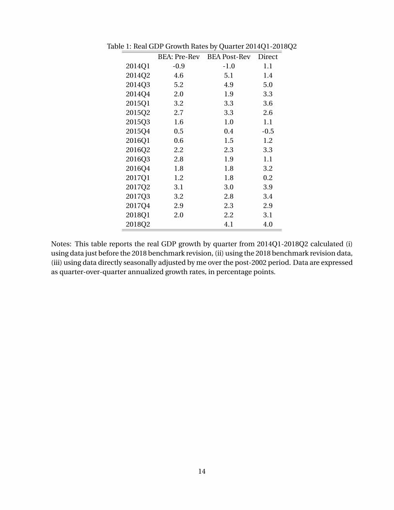
Table 1: Real GDP Growth Rates by Quarter 2014Q1-2018Q2

BEA: Pre-Rev BEA Post-Rev Direct2014Q1 -0.9 -1.0 1.12014Q2 4.6 5.1 1.42014Q3 5.2 4.9 5.02014Q4 2.0 1.9 3.32015Q1 3.2 3.3 3.62015Q2 2.7 3.3 2.62015Q3 1.6 1.0 1.12015Q4 0.5 0.4 -0.52016Q1 0.6 1.5 1.22016Q2 2.2 2.3 3.32016Q3 2.8 1.9 1.12016Q4 1.8 1.8 3.22017Q1 1.2 1.8 0.22017Q2 3.1 3.0 3.92017Q3 3.2 2.8 3.42017Q4 2.9 2.3 2.92018Q1 2.0 2.2 3.12018Q2 4.1 4.0

Notes: This table reports the real GDP growth by quarter from 2014Q1-2018Q2 calculated (i)using data just before the 2018 benchmark revision, (ii) using the 2018 benchmark revision data,(iii) using data directly seasonally adjusted by me over the post-2002 period. Data are expressedas quarter-over-quarter annualized growth rates, in percentage points.

14

Table 2: Average Growth Rates by Quarter: 2002Q1-2018Q1

BEA: Pre-Revision BEA: Post-Revision Direct SAQ1 Q2 Q3 Q4 Q1 Q2 Q3 Q4 Q1 Q2 Q3 Q4

Real GDP 1.1 2.4 2.4 1.8 1.5 2.4 2.2 1.9 2.1 2.0 2.1 2.1Consumption 2.0 2.2 2.4 2.2 2.0 2.2 2.6 2.1 2.2 2.2 2.2 2.2

Durables 4.3 5.9 7.3 2.7 4.1 5.4 7.4 2.4 5.8 5.4 3.8 3.9Nondurables 2.0 1.5 1.6 2.8 2.1 1.3 1.5 2.3 2.2 2.1 2.0 1.3Services 1.6 1.8 1.9 2.1 1.6 1.9 2.1 2.1 1.9 1.9 2.0 1.9

GPDI 0.3 3.9 3.4 3.7 1.1 4.5 4.1 4.2 3.2 3.0 3.6 4.7Structures 0.9 5.9 0.5 -1.7 2.6 5.5 5.4 2.4 1.8 0.5 0.9 1.3Equipment 3.5 4.8 6.7 2.3 -0.5 6.1 1.2 -1.4 5.9 4.6 5.0 5.8Int Prop 3.8 3.6 4.5 4.1 4.1 6.2 8.2 2.9 4.9 4.6 4.8 4.8Residential 0.1 1.4 -0.5 1.3 3.9 4.8 5.3 5.5 -0.1 3.1 -0.8 -0.1

Exports 2.0 6.1 4.0 6.6 2.2 6.2 4.4 6.4 5.3 4.0 4.3 5.0Imports 2.2 4.7 3.2 5.2 2.0 4.8 4.7 5.1 3.9 4.2 4.0 4.0Government -0.5 1.9 1.1 -0.1 0.6 1.2 0.3 0.5 0.8 0.7 0.7 0.7

Fed Defense -2.3 5.8 4.0 -0.9 0.9 3.3 0.5 1.0 1.4 1.6 1.6 1.3Fed Non Defense 3.3 1.5 0.7 2.5 3.4 1.7 0.9 2.8 2.0 2.6 2.5 2.3State and Local -0.5 0.7 0.1 -0.2 -0.2 0.4 0.1 -0.1 0.3 0.0 0.1 0.2

Price IndicesGDP 2.1 2.0 2.0 1.7 1.8 2.0 2.1 1.8 1.9 2.0 1.9 1.9

PCE 1.8 2.1 2.2 1.4 1.8 2.1 2.1 1.4 2.0 1.9 1.9 1.6Core PCE 1.8 1.9 1.7 1.6 1.8 1.8 1.6 1.7

Notes: This table reports the average values by quarter from 2002Q1-2018Q1 of 19 series as de-scribed in the text. GPDI stands for Gross Private Domestic Investment and Int Prop stands forIntellectual Property. For each series, the averages are calculated (i) using data just before the2018 benchmark revision, (ii) using the 2018 benchmark revision data, (iii) using data directlyseasonally adjusted by me over the post-2002 period. All series are expressed as quarter-over-quarter annualized growth rates, in percentage points. Core PCE is not available for the directseasonal adjustment because it is not published in NSA form.

15

Table 3: Properties of Seasonally Adjusted Series

BEA: Pre-Revision BEA: Post-Revision Direct SASD ρ1 ρ4 SD ρ1 ρ4 SD ρ1 ρ4

Real GDP 2.37 0.45 0.07 2.34 0.41 0.02 2.35 0.46 -0.07Consumption 1.84 0.60 0.28 1.82 0.51 0.27 1.59 0.86 0.37

Durables 7.69 0.15 0.12 7.92 0.14 0.07 6.19 0.50 0.08Nondurables 2.45 0.29 0.20 2.36 0.39 0.24 2.44 0.47 0.21Services 1.31 0.72 0.33 1.25 0.56 0.28 1.12 0.74 0.32

GPDI 12.1 0.48 -0.13 12.5 0.42 -0.14 12.7 0.46 -0.10Structures 14.0 0.46 0.09 7.63 0.65 0.07 12.9 0.65 0.04Equipment 12.4 0.54 -0.04 13.9 0.49 0.07 11.6 0.74 -0.14Int Prop 3.95 0.17 0.00 12.1 0.63 -0.09 3.02 0.49 -0.10Residential 14.9 0.54 0.38 5.10 0.04 -0.03 15.0 0.49 0.43

Exports 8.02 0.42 -0.11 8.13 0.42 -0.09 7.94 0.45 -0.09Imports 8.36 0.53 -0.07 8.20 0.56 -0.08 6.92 0.81 -0.17Government 2.62 0.37 0.49 2.42 0.50 0.40 2.25 0.75 0.37

Fed Defense 8.09 -0.01 0.31 6.18 0.14 0.28 5.03 0.57 0.39Fed Non Defense 5.48 0.19 0.03 5.34 0.16 0.03 6.11 0.37 0.09State and Local 2.14 0.44 0.25 2.24 0.57 0.21 2.37 0.58 0.18

Price IndicesGDP 0.97 0.45 0.36 0.98 0.44 0.33 0.80 0.74 0.41

PCE 1.62 0.29 -0.10 1.69 0.28 -0.09 1.68 0.29 -0.08Core PCE 0.55 0.34 -0.05 0.59 0.34 -0.06

Notes: This table reports the sample standard deviation and first and fourth autocorrelationsfrom 2002Q1-2018Q1 of 19 series as described in the text. GPDI stands for Gross Private Do-mestic Investment and Int Prop stands for Intellectual Property. For each series, the statisticsare calculated (i) using data just before the 2018 benchmark revision, (ii) using the 2018 bench-mark revision data, (iii) using data directly seasonally adjusted by me over the post-2002 period.All series are expressed as quarter-over-quarter annualized growth rates, in percentage points.Core PCE is not available for the direct seasonal adjustment because it is not published in NSAform.

16

Table 4: Wald test p values for residual seasonality

BEA: Pre-Rev BEA Post-Rev DirectReal GDP 0.18 0.66 0.98

Consumption 0.68 0.48 1.00Durables 0.50 0.48 0.74Nondurables 0.45 0.40 0.80Services 0.43 0.34 0.98

GPDI 0.63 0.80 0.95Structures 0.00 0.05 1.00Equipment 0.48 0.00 0.87Int Prop 0.89 0.27 0.94Residential 0.86 0.92 0.79

Exports 0.22 0.27 0.97Imports 0.43 0.42 0.99Government 0.11 0.39 1.00

Fed Defense 0.05 0.34 0.99Fed Non Defense 0.29 0.24 1.00State and Local 0.59 0.81 1.00

Price IndicesGDP 0.26 0.54 0.83

PCE 0.57 0.70 0.68Core PCE 0.22 0.35

Notes: This table reports the p-values from Wald tests for residual seasonality in equation (3.1).GPDI stands for Gross Private Domestic Investment and Int Prop stands for Intellectual Prop-erty. The lag truncation parameter is set to 1.3T 1/2 and the p-values of Kiefer and Vogelsang(2005) are used. The tests are run over the 2002Q1-2018Q1 period, using the three different sea-sonally adjusted series. Core PCE is not available for the direct seasonal adjustment because itis not published in NSA form.

17

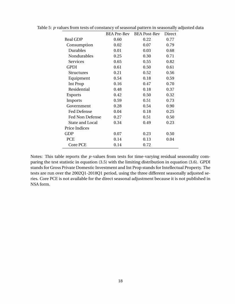
Table 5: p values from tests of constancy of seasonal pattern in seasonally adjusted data

BEA Pre-Rev BEA Post-Rev DirectReal GDP 0.60 0.22 0.77

Consumption 0.02 0.07 0.79Durables 0.01 0.03 0.68Nondurables 0.25 0.30 0.71Services 0.65 0.55 0.82

GPDI 0.61 0.50 0.61Structures 0.21 0.52 0.56Equipment 0.54 0.18 0.59Int Prop 0.16 0.47 0.70Residential 0.48 0.18 0.37

Exports 0.42 0.50 0.32Imports 0.59 0.51 0.73Government 0.28 0.54 0.90

Fed Defense 0.04 0.18 0.25Fed Non Defense 0.27 0.51 0.50State and Local 0.34 0.49 0.23

Price IndicesGDP 0.07 0.23 0.50

PCE 0.14 0.13 0.04Core PCE 0.14 0.72

Notes: This table reports the p-values from tests for time-varying residual seasonality com-paring the test statistic in equation (3.5) with the limiting distribution in equation (3.6). GPDIstands for Gross Private Domestic Investment and Int Prop stands for Intellectual Property. Thetests are run over the 2002Q1-2018Q1 period, using the three different seasonally adjusted se-ries. Core PCE is not available for the direct seasonal adjustment because it is not published inNSA form.

18

Table 6: p values from joint test of stable and zero residual seasonality

BEA Pre-Rev BEA Post-Rev DirectReal GDP 0.19 0.68 1.00

Consumption 0.67 0.47 1.00Durables 0.49 0.47 0.77Nondurables 0.45 0.41 0.82Services 0.45 0.35 0.99

GPDI 0.65 0.83 0.97Structures 0.00 0.06 1.00Equipment 0.50 0.00 0.89Int Prop 0.91 0.27 0.97Residential 0.87 0.94 0.80

Exports 0.22 0.28 0.98Imports 0.44 0.43 1.00Government 0.11 0.39 1.00

Fed Defense 0.05 0.34 0.98Fed Non Defense 0.29 0.25 1.00State and Local 0.61 0.83 1.00

Price IndicesGDP 0.26 0.54 0.85

PCE 0.56 0.69 0.67Core PCE 0.22 0.36

Notes: This table reports the p-values from joint tests of stable and zero residual seasonalitycomparing the test statistic W +L with the limiting distribution in equation (3.7). GPDI standsfor Gross Private Domestic Investment and Int Prop stands for Intellectual Property. The testsare run over the 2002Q1-2018Q1 period, using the three different seasonally adjusted series.Core PCE is not available for the direct seasonal adjustment because it is not published in NSAform.

19

References

BARSKY, R. B., AND J. A. MIRON (1989): “The Seasonal Cycle and the Business Cycle,” Journal ofPolitical Economy, 97, 503–534.

BLOEM, A. M., R. J. DIPPELSMAN, AND N. Ø. MÆHLE (2001): Quarterly National Accounts Man-ual: Concepts, Data Sources, and Compilation. IMF.

BOLDIN, M., AND J. H. WRIGHT (2016): “Weather-Adjusting Economic Data,” Brookings Paperson Economic Activity, 2, 227–278.

CANOVA, F., AND B. E. HANSEN (1995): “Are Seasonal Patterns Constant over Time? A Test forSeasonal Stability,” Journal of Business and Economic Statistics, 13, 237–252.

CHO, C.-K., AND T. J. VOGELSANG (2017): “Fixed-b inference for testing structural change in atime series regression,” Econometrics, 5, 2.

GHYSELS, E. (1988): “A Study Toward a Dynamic Theory of Seasonality for Economic Time Se-ries,” Journal of the American Statistical Association, 83, 168–172.

GILBERT, C., N. J. MORIN, A. D. PACIOREK, AND C. R. SAHM (2015): “Residual Seasonality inGDP,” Board of Governors of the Federal Reserve System, FEDS Notes.

GÓMEZ, V., AND A. MARAVALL (1996): “Programs TRAMO and SEATS. Instructions for the User,”Working Paper 9628, Servicio de Estudios, Banco de España.

(2013): “Automatic modeling methods for univariate time series,” in A Course in TimeSeries Analysis, ed. by D. Peña, G. C. Tiao, and R. S. Tsay. J. Wiley and Sons.

GROEN, J., AND P. RUSSO (2015): “The Myth of First-Quarter Residual Seasonality,” Federal Re-serve Bank of New York, Liberty Street Economics Blog.

HANSEN, L. P., AND T. J. SARGENT (1993): “Seasonality and Approximation Errors in RationalExpectations Models,” Journal of Econometrics, 55, 21–55.

KIEFER, N. M., AND T. J. VOGELSANG (2005): “A new asymptotic theory for heteroskedasticity-autocorrelation robust tests,” Econometric Theory, 21, 1130–1164.

LANDEFELD, J. S., E. P. SESKIN, AND B. M. FRAUMENI (2008): “Taking the Pulse of the Economy:Measuring GDP,” Journal of Economic Perspectives, 22, 193–216.

LAZARUS, E., D. J. LEWIS, J. H. STOCK, AND M. W. WATSON (forthcoming): “HAR Inference:Recommendations for Practice,” Journal of Business and Economic Statistics.

LOTHIAN, J., AND M. MORRY (1978): “A Set of Quality Control Statistics for the X-11 ARIMASeasonal Adjustment Method,” Statistics Canada Working Paper 78-10-005E.

LUNSFORD, K. G. (2017): “Lingering Residual Seasonality in GDP Growth,” Federal ReserveBank of Cleveland, Economic Commentary.

20

MARAVALL, A. (1995): “Unobserved Components in Economic Time Series,” in The Handbookof Applied Econometrics, ed. by H. Pesaran, and M. Wickens. Basil Blackwell.

(2006): “An application of the TRAMO-SEATS automatic procedure; direct versus indi-rect adjustment,” Computational Statistics and Data Analysis, 50.

MCCULLA, S. H., AND S. SMITH (2015): “The 2015 Annual Revision of the National Income andProduct Accounts,” Survey of Current Business, 95:8.

MCDONALD-JOHNSON, K. M., B. MONSELL, R. FESCINA, R. FELDPAUSCH, C. C. H. HOOD,AND M. WROBLEWSKI (2010): “Census Bureau Guideline: Seasonal Adjustment Diagnostics,”Manuscript, US Census Bureau.

MOULTON, B. R., AND B. D. COWAN (2016): “Residual Seasonality in GDP and GDI: Findings andNext Steps,” Survey of Current Business, 96:7.

NYBLOM, J. (1989): “Testing for the Constancy of Parameters Over Time,” Journal of the Ameri-can Statistifcal Association, 84, 223–230.

PENEVA, E. (2014): “Residual Seasonality in Core Consumer Price Inflation,” Board of Governorsof the Federal Reserve System, FEDS Notes.

PHILLIPS, K. R., AND J. WANG (2016): “Residual Seasonality in U.S. GDP Data,” Federal ReserveBank of Dallas Working Paper 1608.

RUDEBUSCH, G. D., D. WILSON, AND T. MAHEDY (2015): “The Puzzle of Weak First-Quarter GDPGrowth,” Federal Reserve Bank of San Francisco, Economic Letter.

SAIJO, H. (2013): “Estimating DSGE models using seasonally adjusted and unadjusted data,”Journal of Econometrics, 173, 22–35.

SIMS, C. A. (1993): “Rational Expectations Modeling with Seasonally Adjusted Data,” Journal ofEconometrics, 55, 9–19.

STARK, T. (2015): “First Quarters in the National Income and Product Accounts,” Federal Re-serve Bank of Philadelphia, Research Rap Special Report.

WRIGHT, J. H. (2013): “Unseasonal Seasonals?,” Brookings Papers on Economic Activity, 2, 65–110.

(2017): “Optimal Seasonal Filtering,” Manuscript, Johns Hopkins University.

21