Prior Modelling and Posterior sampling in Impedance Imaging

G. K. Nicholls and C. Fox

Mathematics Department, The University of Auckland, Auckland, New Zealand

ABSTRACT

We examine sample based Bayesian inference from impedance imaging data. We report experiments employing lowlevel pixel based priors with mixed discrete and continuous conductivities. Sampling is carried out using Metropolis-Hastings Markov chain Monte Carlo, employing both large scale, Langevin updates, and state-adaptive local updates.Computing likelihood ratios of conductivity distributions involves solving a second order linear partial dierentialequation. However our simulation is rendered computationally tractable by an update procedure which employs alinearization of the forward map and thereby avoids solving the PDE for those updates which are rejected.

Keywords: Impedance tomography, Markov chain Monte Carlo, Bayesian, Langevin, Inverse problem

1. INTRODUCTION

Conductivity imaging, also known as electrical impedance tomography (EIT), is not yet established as a workableimaging technique. The best reconstructions obtained to date1 have very low resolution and are hard to interpret.The question is, is this low resolving power an inherent weakness of the physical imaging process, or is it an artifactof the data analysis. We are unable to give a nal answer, since we have not yet obtained real data for trial analysis.However our experiments with synthetic data, which we present below, indicate substantial improvements on existinginversion methods are to be made.

We begin by dening the physical imaging process. Referring to Figure 1(a), electrodes are placed in contactwith an object, and a small current is applied through some of these electrodes. One of the non-current electrodes isselected as a reference electrode, and the potential dierence between each of the remaining non-current electrodesand the reference is measured in volts. These measured potential dierences depend on the unknown conductivitydistribution of material inside the object. In conductivity imaging we attempt to reconstruct the conductivity ateach point in the object using the known currents and the observed potentials.

The denitions which follow are from Fox and Nicholls.2 Consider the two-dimensional region, with boundary@ shown in Figure 1(a). The conductivity (units ohms1) is an unknown function of position, (x); x 2 , in theregion. It may in practice be bounded above and below so that 0 < min (x) max <1. Electrodes producingxed current source distributions J@ = J@(x) for x 2 @ and J = J(x) for x 2 are applied at the boundaryand in the interior of the region. The dimensions of J@ and J are current per unit length and current per unit arearespectively. The electrical potential, , is measured along the boundary. Within the region the potential satisesthe partial dierential equation

r (r) = J: (1)

If the region is otherwise insulated, the current crossing @ is just J@. Hence if nx is the unit outward normal onthe boundary @, the boundary current density is

@

@nx= J@: (2)

Suppose K electrodes are attached at the boundary of a region at points xk 2 @; k = 1; 2 : : :K. LetE = fx1; x2 : : : xKg be the set of electrode positions. A pair of electrodes are chosen as anode and cathode and acurrent of magnitude I0 is applied. A third reference electrode is chosen, and a voltmeter is connected between thereference electrode and each of the other electrodes in turn, not including the anode and cathode, and a potentialis measured. Let ean; e

cn and ern denote respectively the label of the anode, cathode, and reference electrode used in

each of the n = 1; 2 : : :N electrode arrangements, and let en = fean; ecn; erng. Since there are N = K(K1)=2 distinct

CF: E-mail: fox@math.auckland.ac.nz, GKN: E-mail: nicholls@math.auckland.ac.nz

Further info at http://www.math.auckland.ac.nz/nicholls/linkfiles/papers.html

x

x

2

4

3

Κ−1 Κ

1

reference

0510152025

010

2030

−1.5

−1

−0.5

0

0.5

1

xσ(

Ω

)

Ω

V

J

A B C

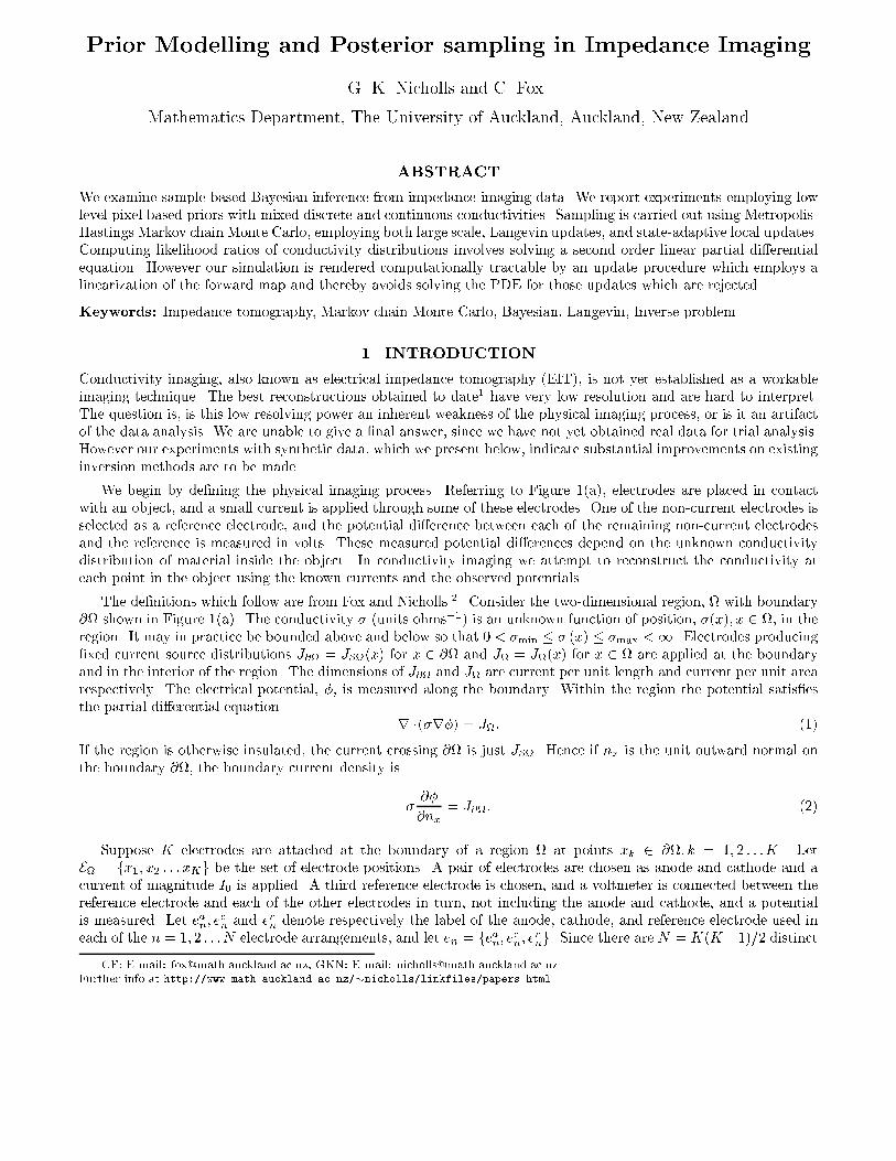
Figure 1. (a) Region of spatially varying conductivity and with bounding curve @. The choice of anode, cathodeand reference electrode shown corresponds to the choice ean = 1; ecn = 2 and ern = 3. The full measurement set is madeup of all electrode potentials, measured in turn for all distinct choices of anode and cathode. The index n indicatesa set of measurements associated with some particular choice of anode and cathode. (b) Electrode positions used inthe experiments section. The graph in (c) is the potential eld (xjn; s) for the conductivity of Figure 3(a), for oneof the n = 1; 2 : : : 120 electrode arrangements.

anode-cathode choices, we measure N , K 3 component vectors, vn; n = 1; 2 : : :N . Let the current due to the n'thelectrode pair be Jn = fJ;n; J@;ng. The electrodes are modelled as point sources of magnitude I0, located in theinterior, so J@;n(x) = 0 and

J;n(x) = I0(x xean) I0(x xec

n): (3)

We measure one vector vn for each of the current distributions J1; : : : JN generated by the N distinct current electrodepairs. Note that these measurements are not all independent. We have a total of (K 3) K(K 1)=2 values inall, while only K(K 1)=2 are independent, as we will see. For notational convenience we let vn be a K componentvector, so that vn(k) is the potential measured at the kth electrode in the nth electrode conguration. The redundantcomponents vn(k) k 2 en are left undened.

Let s(x) be the true conductivity at each point x 2 , and let (xjn; s) be the potential at x generated by currentdistribution Jn in the conductivity s. Refer to Figure 1(c) for the potential function of an applied current distributionin the conductivity of Figure 3(a). Let (s) denote the N component vector of functions ((xj1; s); : : : (xjN; s)).We suppose the voltage measurements are made in noise that is independent, additive and Gaussian, mean zeroand standard deviation d, whilst currents are measured exactly. Thus if n(k) is a Gaussian random variable,n(k) N(0; d2), we observe

vn(k) = (xk jn; s) + n(k); for each n = 1::N; k = 1::K; k 62 en: (4)

The potential at the reference electrode is (xernjn; s) 0. The solution to the PDE, Equation (1), is determined

only up to an additive constant, and by setting (xernjn; s) = 0 we fully determine the solution. Now, given applied

currents J = (J1; : : : JN ) and data v = (v1; : : : vN ), the likelihood of a conductivity distribution (x) is proportionalto exp(L(jv; J)), where L() L(jv; J) is the log-likelihood, up to a term independent of ,

L() = jv ()j=2d2; with jv ()j NXn=1

KXk=1

k 62en

(vn(k) (xk jn; ))2: (5)

In order to compute the likelihood, we must solve Equations (1) and (2) for (xjn; ),rx (rx(xjn; )) = I0(x xea

n) I0(x xec

n) (6)

with@(xjn; )=@nx = 0; (7)

for each n = 1; 2 : : :N . The posterior for a conductivity distribution , given observations v, generated by currentsJ , is then Prfs 2 djv; Jg / Prfs 2 dg exp(L(jv; J)). We intend to sample the distribution Prfs 2 djv; Jg anduse these samples to answer questions concerning the unknown true conductivity s.

2. PROPERTIES OF THE INVERSE PROBLEM

For a xed conductivity (x) and for interior sources J, the Dirichlet boundary value problem r (r) = Jin subject to boundary conditions j@ = V has a unique solution, , which has current crossing the boundary

equal to J@ = @@n . The map : V 7! J@ is called the Dirichlet to Neumann map for given (and J). Notethat the dierential equation is linear in and, hence, so is . However, the relationship between and is notlinear. The forward problem is then to determine given . One simply solves the PDE. The inverse problem is:determine from incomplete measurements (J;n; J@;n; vn)

Nn=1 of .

A number of existence and uniqueness results3 hold for the inverse image of the nonlinear forward map, 7! .However, the issue of uniqueness of the inverse, per se, is not of practical importance and greater insight may begained by examining the singular value decomposition (SVD) of the the linearised forward problem. The right-and left-singular vectors give the bases of conductivity and data, respectively, in which the linearised forward mapis diagonalised and hence reduced to component-wise multiplication by the singular values. With respect to thosebases, the singular values give the magnitude of the directional derivative of the forward map in each coordinatedirection and hence give the sensitivity of the forward map to small changes in conductivity.

The linearised forward map for imaging the conductivity of a disc, assuming complete measurement of , hasbeen shown to have singular values that are arbitrarily close to zero4 and hence the inverse is discontinuous. So theidealised inverse problem is ill-posed. In the practical case of reconstructing a pixelised version of from a nitenumber of data, the decreasing singular values cause the inverse problem to be very badly conditioned. For imagingthe conductivity of a disc which is close to homogeneous, with measurement accuracy of 0.1%, about 140 singularvalues exceed the threshold mentioned above and thus there are about 140 independent structures of the conductivityabout which measurements can be made.4 Thus if direct inversion of the forward problem is attempted, any imagewith more than 140 pixels must have correlations between pixels that are solely functions of the particular noiserealisation and those spurious structures will tend to be large as a result of the small singular values. On the otherhand, reconstructing an image of conductivity with few pixels, e.g. 140, will not give good reconstructions as theforward problem is poorly approximated unless the true conductivity happens to be piece-wise constant with thesame structure as the pixilation.

3. PREVIOUS APPROACHES TO CONDUCTIVITY IMAGING

Despite the inverse problem being very badly conditioned, with a theoretically discontinuous inverse, the vast majorityof eort into conductivity imaging has been to implement algorithms that seek to simply invert the forward operator.It is not surprising, therefore, that the literature contains a conspicuous paucity of reconstructed images.

A review paper5 in 1989 Barber outlined a number of the direct-inversion schemes tried to that date. All ofthose schemes sought to directly invert using a single, or iterated, inversion of an approximation to the nonlinearforward map, 7! , with the approximation relying on a single trial value of conductivity. An obviously goodchoice for an approximation to the forward map is a local linearisation about a known conductivity as given by theFrechet derivative. However, even though this linearisation was known early on,6 many early algorithms used ad

hoc approximate inverses often loosely based on `back-projection' as used in x-ray tomography.

More promising have been the direct inversion schemes using a local linearisation of the nonlinear forward mapto iterate towards a solution. Barber concludes that Yorkey's7 method was the best. Yorkey's method does notemploy a global regulariser on the reconstructed solution, but only a local regulariser on each linearised step. Whenexamined in detail, almost all of the iterative algorithms can be found to regularise the inversion of the forward mapimplicitly in the numerical scheme used as opposed to the desirable situation of having an explicitly chosen meansof dealing with the ill-posedness.

In the statistical framework, the direct solution of the inverse problem is a ML estimate and suers from allthe usual problems when the forward mapping has a large range of sensitivities such as the reconstructed imageconsisting mainly of amplied noise. But a deeper problem with the algorithms outlined can be seen through each ofthem being equivalent to some gradient-based algorithm for maximising the likelihood or some implicitly modiedlikelihood. Gradient-based methods require the space of allowable solutions to be connected and convex becauseiteration is performed by moving along search directions derived from local information. Thus it is very dicult toinclude high-level prior information such as \the conductivity at each point is one of ve values" or \the image is anite number of circular regions", etc, as would be desirable.

Since 1990 a number of authors have recognised that the inverse problem requires global regularisation and haveoptimised an appropriately modied objective function. An example of classical regularisation within an iterativescheme is given by Hua et al.8 who propose using Sobolev-type norms as regularisers and provide results using the rstof these, namely the square-norm of the conductivity, using a Newton-Raphson technique to perform the resultingoptimization. Recently, Martin and Idier9 have compared Hua et al.'s method with one using a Markov random eld asprior within a Bayesian statement of the inverse problem. They used the sum of the convex Huber penalty functionof nearest-neighbour dierences for their log-prior and calculated a MAP estimate (from an improper posterior)using a gradient based optimiser. Since their prior prefers local smoothness with discontinuities, the reconstructionsprovided of conductivities of this type are improved. As far as the present authors are aware, the few other Bayesianformulations of conductivity imaging have been restricted to calculating MAP estimates with low-level priors andare, therefore, not fundamentally dierent to regularised inversion.

4. COMPUTING THE LIKELIHOOD

Let current distributions J = (J1; J2 : : : JN ) and a conductivity be given. In order to compute the likelihood of, we need the elds (xjn; ) for x 2 E. That is, we need the eld at the electrodes only. Let g(xjy; ) be theNeumann Green's function for the potential at x 2 given a point-like current source located at y 2 , with auniform current sink along the boundary. That is, g(xjy; ) satises the PDE

rx (rxg(xjy; )) = (2)(x y) (8)

with@g(xjy; )=@nx = 1=j@j; (9)

where j@j is the length of the boundary. The Green's function is determined up to an additive constant. We xthis by referring our Green's functions to a mean zero voltage over the boundary, that is, we imposeZ

@

g(xjy; ) d`(x) = 0: (10)

where d`(x) is the element of length measure along @. It is straightforward to show that the Green's functions wehave dened are symmetric, ie, g(yjx; ) = g(xjy; ), although this depends delicately on the boundary conditions,Equation (9), and on the choice of reference potential made in Equation (10).

Since the potential elds, (xjn; ), n = 1; 2 : : :N , satisfy Equations (6) and (7), they are given in terms of theGreen's functions by

(xjn; ) =

Z

g(xjy; )J;n(y) d(y) +Z@

g(xjy; )J@;n(y) d`(y) 0(xernjn; )

= I0g(xjxean; ) I0g(xjxec

n; ) 0(xer

njn; ) (11)

using Equation (3), where d(x) is the element of area measure in , and

0(xernjn; ) I0g(xer

njxea

n; ) I0g(xer

njxec

n; ):

We subtract 0(xernjn; ) so that the potential at the reference electrode located at xer

nis zero. It follows that, in order

to compute the N = K(K 1)=2 elds (xjn; ), we must compute K Green's functions, g(xjxk; ); k = 1; 2 : : :K,one for each point, xk, at which we attach an anode or cathode. The potential elds are given as linear combinationsof this set of \fundamental solutions" by Equation (11). Since the elds we measure depend on just K Green'sfunctions, no potential measurement can be made at the source electrode, and the Greens functions are symmetric,K(K 1)=2 is the number of genuinely independent measurements that can be made on K electrodes.

In the examples which follow, we solve for the Green's functions in a square region. We discretise the region in anM -element regular square array (mesh) of pixels labelledm = 1; 2 : : :M assigning the pixel conductivity m accordingto conductivity at the center of the pixel. Thus the conductivity (x), the elds (xjn; ), and the Green's functionsg(xjy; ) have corresponding discrete representations m, m(n; ) and gm

0

m () satisfying dierence equations andsummation conditions derived in the simplest possible way from Equations (8), (9) and Equation (10). Note thatwe represent the conductivity in on the same square mesh we use to solve for (), using the same symbol forthe vector of lattice values m, m 2 1; 2 : : :M and the distribution function (x), x 2 . For the results presented asimple nite dierence scheme was implemented in C and called to solve for the Green's functions.

5. MODELLING THE CONDUCTIVITY

We wish to specify a prior distribution for the probability that some trial conductivity coincides with the unknowntrue conductivity s in . We must specify model variables, their state space, and probability distribution or density.These prior models may also be regarded as representing varying states of prior knowledge. In this paper we presentresults for Models A and B. See the conclusions for further remarks concerning Model C.

Model A There are C possible types of material in the region. The conductivities of the materials are known exactly,and correspond to the values C = fC1; C2 : : : CCg. In this case m 2 C. We model on the lattice as an Isingor Potts binary or higher order Markov random eld, with distribution

Prfs = g / exp

MXm=1

Hm()

!where Hm()

Xm0m

m;m0 :

The sum overm0 m is a sum over the four immediate neighbours m0 of m on the square lattice. The functiona;b is the indicator function for the event a = b. Let A = CM denote the set of all possible pixel-basedconductivity distributions in model A so that in model A, 2 A .

Model B The types of possible materials (labelled 1; 2 : : :C) making up the object are known. However, the con-ductivities of these materials vary from pixel to pixel within . Let (x); x 2 be some estimate of thematerial type eld. Corresponding lattice variables m, m = 1; 2 : : : ;M with state space m 2 f1; 2 : : :Cg givethe estimated material type at pixel m. Let t(x); x 2 denote the unknown true material type eld in .Let B = f<+gM and TB = f1; 2 : : :CgM denote the state space of and in model B, so that in modelB, 2 B and 2 TB . Let d = d1d2 : : : dM . Conditional on the material type , we suppose that theprior distribution of is multivariate normal, subject to the condition m > 0;m = 1; 2 : : : ;M , with mean() and variance () depending on the material type, and correlation parameter ~. Let N0(r;; ) denotethe normal density, mean , variance , but normalised over r > 0 only. Conditional on material type the priordistribution is then

Prfs 2 djg / exp

~

MXm=1

Gm()

!

MYm0=1

N0(m0 ;(m0); (m0)) d where Gm() X

m00m

(mm00)2

In this model the C parameters (c); c 2 f1; 2 : : :Cg replace the C parameters fC1; C2 : : : CCg of model A. Theeld representing the spatial distribution of material type has a Potts or Ising prior Prft = g, identical toPrfs = g in model A. The overall prior is Prft = ; s 2 dg = Prft = gPrfs 2 djg.

Model C We may, in addition, have knowledge about the structure, shape, and arrangement of objects in the region.For example it may be known to contain man-made objects, with outlines that are composed of simple polygonalstructures. An intermediate level prior, modelling the underlying continuum process10,11 is appropriate.

6. MARKOV CHAIN MONTE CARLO

We wish to sample the posterior distributions obtained under models A and B. Model A may be regarded as aspecial case of B in which ~ = 0 and (i) is very small compared to j(i) (i1)j and j(i+1) (i)j for eachi = 1; 2 : : :C. We dene a Markov chain fXng1n=0 of random variables Xn taking values in B TB , and having an

n-step distribution with the property limn!1PrfXn 2 (; d)jX0 = ( (0); (0))g = Prft = ; s 2 djvg. Such a process

will generate the samples we require. We use Metropolis-Hastings updates. In order to get ergodic behaviour onuseful time scales we found it necessary to include several dierent types of update or move-types in the MCMC. Amove is a stochastic operation used to determine a value for Xn+1 given a value for Xn.

The simplest way to build multiple moves into a Metropolis-Hastings sampler is to dene a separate reversible tran-sition probability for each move type.12 Let P be the number of moves, and let fPr(p)fXn+1 2 (n+1; dn+1)jXn =(n; n)ggPp=1 be a set of P transition probabilities, reversible with respect to the posterior distribution Prf; djv; Jg.Let p; p = 1; 2 : : : P be the probability to choose move p. Necessarily,

Pp = 1. We select move p with probability

p and use it to generate a MCMC update. The overall transition probability is

PrfXn+1 2 (n+1; dn+1)jXn = (n; n)g =PXp=1

p Pr(p)fXn+1 2 (n+1; dn+1)jXn = (n; n)g:

If at least one of the moves is Prf; djv; Jg-irreducible on B TB , then the equilibrium distribution of the chainis Prf; djv; Jg,13 independent of X0, the MCMC initialisation. We list the moves used in an Appendix A.

Assertion For each p = 1; 2 : : :7 let

Pr(p)fXn+1 2 (n+1; dn+1)jXn=(n; n)g qp( (; )! ( 0; d0) ) p( (; )! ( 0; 0) )

for qp((; )! ( 0; d0)) and p((; )! ( 0; 0)) the proposal and acceptance distributions dened in Appendix A.

For each p = 1; 2 : : : 7, the transition kernel Pr(p)fXn+1 2 (n+1; dn+1)jXn = (n; n)g is reversible with respect toPrf; djv; Jg. Also, the transition kernel for move 1 denes a process Prf; djv; Jg-irreducible on B TB .

7. MARKOV CHAIN MONTE CARLO WITH AN EIT LIKELIHOOD

In this section we refer to a \current" process state, Xn = (; ), and a \candidate" state, labelled ( 0; 0), proposedin the course of a Metropolis-Hastings update. In order to compute the acceptance probabilities, p, at an update,we need L(0)=L(). As we saw in Section 4, this involves solving Equations (8) and (9) for the Green's functionsg(xjxk ; 0) in the candidate conductivity 0, and computing (xjn; 0) and L(0) using Equations (11) and (5). Wehave described how we solve for the Green's functions. This operation takes too much time to be feasible at eachstep of the Markov chain. Notice, however, that for moves 1-4, at least, the two conductivities and 0 dier onlyslightly, and that we have already calculated the Green's functions g(xjxk ; ) in the current conductivity . In aprevious paper2 we have shown how the Green's functions for may be used to estimate the Green's functions in0, and therefore the log-likelihood L(0). Our estimate is good when 0 and dier only slightly.

The MCMC algorithm is as follows. Given a state Xn = (; ), given the Green's functions g(xjxk ; ), for x 2 and xk 2 E, k = 1; 2 : : :K, and given L(), the log-likelihood of the state, Xn+1 is determined in the following way.

Step I Select a move p with probability p. Generate (0; 0) by sampling qp((; ) ! ( 0; d0)).

Step II Using the local linearization,2 estimate L(0).

Step III Compute the acceptance probability for the state, p((; ) ! ( 0; 0)).

Step IV Accept or reject the candidate state ( 0; 0):

IV.i If ( 0; 0) is rejected, set Xt+1 = . There is no change to the state so the Green's functions andlog-likelihood are unchanged, available for the next iteration.

IV.ii If ( 0; 0) is accepted, set Xt+1 = 0. We must now solve Equations (8) and (9) K times in order tocompute g(xjxk ; 0), for k = 1; 2 : : :K, and update the log-likelihood to L(0).

To summarise, given the Green's functions for current sources in a conductivity , we may estimate the likelihoodof a candidate conductivity 0 generated in the Metropolis-Hastings procedure, without solving the PDE again.Metropolis-Hastings updates which lead to rejection are local operations, involving the conductivity values at just afew pixels neighbouring the point at which a change is made. However, if 0 is accepted, we must solve the PDE, aswe now wish to perturb about the elds of the conductivity 0.

We conclude with a comment on computing the Metropolised Langevin update. Referring to Equation (13),the key computation is of @(xk jn; )=@m. We must compute the change in the eld at electrodes caused by asmall change in the conductivity within the region. This is eected without solving the PDE, in a computation oforder constant in time for each m, using the same linearisation as before2 to compute the response of the Green'sfunctions to a small change in at each pixel m = 1; 2 : : :M in turn. In a process in which the computation oflikelihood ratios is expensive, \large" updates, involving changes to a large number of pixels, become attractive.Usually such moves are not feasible, as randomly generated candidate states tend to have low probability, andare therefore rejected. However Langevin updates generate candidate states which step in the direction of locallydecreasing posterior potential, leading to acceptable acceptance rates if the jump size h is chosen appropriately.14

In the process we dene, the Langevin update has a very low acceptance rate for reasonable h values, probably onaccount of the extreme sensitivity of the likelihood to variations in the conductivity near the boundary. It may beappropriate to normalise the Langevin update vector r log(f(; jv)), or work with a spatially varying parameter h.Either revision is straightforward in a Metropolis adjusted diusion. Other schemes exist for selecting large updateswhich have good acceptance rates, notably micro-canonical updates.15

8. EXPERIMENTS

The algorithm described in Section 7 was implemented in C. The MCMC software was tested in the usual way.2

In each of the following examples we start with a known, or \true", conductivity distribution, s(x). This is imagedwith 16 electrodes located as shown in Figure 1(b). The conductivity model and the nite dierence PDE solveruse the same 25 25 conductivity lattice. We condition on the value of the conductivity around the electrodes, soXn(x) = s(x) for all n = 0; 1; 2 : : : and all x inside a strip of width 2 pixels neighbouring the border. Details of all theexperiments we present are shown in Table 1. Articial data v is generated by adding Gaussian noise to the potentialobserved at each electrode, as in Equation (4). We choose to test observations with standard deviation d = 0:005, asignal to noise ratio of around 1500 : 1, taking account of the (K 3)-fold over-measurement. Measurements of thisquality are physically achievable.

We sample the posterior with Markov Chain Monte Carlo, initialising the chain in all cases with a random patternof conductivity (and material types, Model B and Figure 4). We compute the mean and variance of the sampledconductivity at each pixel. These statistics are displayed as images, along with a sample from the posterior, inthe gures which follow. The sample we present is simply the state of the MCMC process at the end of a longsequence of updates of xed length. A number of statistics are recorded along the run, including the log-likelihoodL(), the posterior potential, and the proportion of pixels of each conductivity value (Model A) or type (Model B).Convergence is rather slow, though it seems to be reliable, as can be judged from the output statistics plotted inFigure 2. The integrated autocorrelation time (IACT) of the log-likelihood (LL say) was computed. This quantityis small in ecient MCMC. Roughly speaking, LL is the number of correlated MCMC samples from the posteriorwith the variance-reducing power of one independent sample. We nd that the IACT does indeed drop when moves5 and 6 are included alongside moves 1-4.

In the experiment from the synthetic data of Figure 3(a), three conductivity values (C1 = 1, C2 = 2 and C2 = 3)appear. Referring to the variance image, Figure 3(d), the reconstruction of the square region with conductivity value2 units is somewhat uncertain. The data may now be tted by replacing part of this region by a small region in whichthe conductivity value is 2 units, and shrinking it somewhat. In an earlier experiment (presented elsewhere2), treatingsynthetic binary conductivity patterns, observed under the same conditions as here, and reconstructed using the priorknowledge of Model A, we found we were able to recover (x) essentially perfectly, and with negligible variation inthe posterior conductivities at pixels. The uncertainty in the recovered conductivity distribution increases as thenumber of allowed conductivity levels increases, as Figure 3 shows. However, the mean conductivity remains a goodestimator for the true conductivity s(x).

When we move to the more realistic state of prior knowledge represented by Model B, the ambiguity in thereconstruction increases again. The simulation summarised in Figure 4 illustrates this observation. The prior

Table 1. Run parameters for gures. Blank entries are not applicable or not of interest. The second row correspondsto a run sampling the same posterior distribution as in the rst row, but with varied move proportions.

Figure Model move fractions % ; ~ (1); (2); (3) (1); (2); (3)1 : 2 : 3 : 4 : 5 : 6 or C1; C2; C3

3 A 1:9:50:40:0:0 0.75,- 1.0, 2.0, 3.0 - - -(no image) A 1:9:40:40:5:5 0.75,- 1.0, 2.0, 3.0 - - -4 B 1:9:40:40:0:0 0.0,0.5 1.0, 2.0, 3.0 0.2 0.2 0.25 A 1:9:40:40:5:5 0.75,- 1.0, 2.0, 3.0 - - -

Table 2. Output statistics for Figures. Missing entries are not applicable or not of interest. Bracketed quantitiesindicate standard errors. The rst two rows repeat the same simulation with varied move proportions. This is doneto test the algorithm implementation. Estimated means, EfL()g, should agree. 1 sweep is 441 updates, the numberof pixels in the lattice which are subject to updates. LL is the IACT of the log-likelihood, see text. Timing is givenfor a simple serial C-implementation of the sampling algorithm on a machine with SPECfp95 equal 12.4

Figure LL sweeps LL minutes EfL()g3 (a-d) 100(10) sweeps 4 -810.9 (0.1)3 (no image) 45(10) sweeps 10 -811.0 (0.2)4 (g,h,i,j) 170(40) sweeps 5.5 -

0 2000 4000 6000 8000 10000Lag in sweeps

−0.25

0.25

0.75

ACF

0 50000 100000 150000 200000MCMC updates in sweeps

−880

−860

−840

−820

−800

−780

L(σ)

0 2000 4000 6000 8000 10000Lag in sweeps

−0.25

0.25

0.75

0 20000 40000 60000 80000MCMC updates in sweeps

−950

−900

−850

−800

A C

B D

Figure 2. The sample log-likelihood (up to a constant independent of ) plotted against the update number, alongwith the autocorrelation function (ACF) of the MCMC output series. (A) Model A, series used to estimate resultsin Figure 3. (B) ACF of series in (A). Dashed lines indicate variance of ACF asymptotic in the lag. (C) Model B,for Figure 4g-j. (D) ACF of series in (C). Otherwise as for (B). The quality of convergence in Figure 4g-j is poor ascan be seen from (D).

DA B C

Figure 3. Recovering conductivity information for a synthetic data set with three conductivity levels, computedfrom (a), electrode positions as in Figure 1a. Conductivities C1; C2 and C3 are black grey and white respectively.The state in (b) is a sample from the posterior, the mean conductivity is shown in (c), and pixel conductivity varianceis shown in (d), where darker shades indicate greater variance.

A B C D E

Figure 4. Recovering conductivity information for a synthetic data set, computed from (a) with continuous, varying,conductivity pixel variables. Lighter shades indicate higher conductivity. Material type as for Figure 3(a). The statein (b) gives sampled reconstructed material type classications while (c) gives sampled reconstructed conductivityvalues. Mean conductivity values are shown in (d), and pixel conductivity variance is shown in (e).

A B C

E

D

HF G

Figure 5. Indications of shielding leading to increased uncertainty in sampled reconstructed conductivity. Recov-ering conductivity information for a synthetic data set with three conductivity levels. (a) gives true conductivity for(b)-(d), (e) gives true conductivity for (f)-(h). (a,e) true conductivity, (b,f) sample reconstructed conductivity fromposterior, (c,g) mean conductivity and (d,h) pixel conductivity variance.

knowledge of material type correlation between adjacent pixels becomes important in lowering the probability ofreconstructions in which the border of blocks of uniform material type loose denition. We nd we are able tosample the posterior adequately using moves 1-4. However, the state-adaptivity of moves 1-4 is important. Simplermove sets not focusing on the discontinuity set of the type eld prove to be inadequate.16

Finally, certain patterns of conductivity can screen internal structure. The true conductivity distributions shownin Figures 5(a) and (e) are similar, except that in (a) the conductivity levels on an inward bound path go medium-low-high (ie, 2:0 1:0 3:0) whilst in (e) the sequence is low-medium-high (ie, 1:0 2:0 3:0). The lack of contrastin the interior makes the conductivity distribution of Figure 5(e) relatively dicult to reconstruct. The posteriorvariance is large in the interior, and the structure there is determined largely by the prior.

9. CONCLUSIONS

We nd that a Bayesian approach to inverting EIT data, with analysis based on posterior samples obtained viaMCMC simulation, is feasible, for simple synthetic problems. This is a promising result. It suggests that it will bepossible to explore real EIT data using well developed statistical methods and visualisation devices. A relativelysophisticated adaptive sampling algorithm is required. This algorithm is modular, ie built of separate move types.Its main elements will be useful in MCMC outside Bayesian EIT. The high computational cost of an acceptance inour MCMC algorithm is balanced against the more common but faster rejections. The PDE need only be solved inthe event that an update is accepted. Thus we found moves 1-4 adequate for sampling despite an overall acceptancerate around 2%. Moves 5 and 6, which use sub-chains of MCMC updates, are expensive to compute. They solveinitial convergence problems in certain dicult (low-noise) examples we have explored.

We expect that higher level models, of the kind described in Section 5, Model C, and explicitly elsewhere inthis conference, will resolve these problems in a more general way, for at least some electrode arrangements andconductivity distributions. Higher level models remove or change the character of the ambiguity in the reconstruction.This ambiguity corresponds to multi-modality in the posterior, which is the immediate diculty. Ambiguities causedby screening also may be ameliorated if extra high level information is available. Our own initial experiments inthis line with relatively complex intermediate level (continuum mosaic11,17) models have themselves shown poorconvergence. We expect that simpler continuum models18 will be more eective.

APPENDIX A. MARKOV CHAIN MONTE CARLO UPDATES

In this Appendix we detail the moves used to dene the MCMC. Each move denes a transition kernel reversiblewith respect to the posterior distribution. The state is composed of regions of uniform conductivity. Referring to

Figure 3(d), we see that much of the uncertainty in the reconstructed state occurs at change points in the conductivity.We therefore construct moves which focus updates on pixels in regions where the conductivity is non-uniform.19 Theexpressions for the acceptance probabilities p, p = 1; 2 : : :7 given for the following moves are calculated using theusual Metropolis-Hastings formula.20

A pixel n is a near-neighbour of pixel m if their lattice distance is less thanp8. A pixel has twenty four near-

neighbours, unless it is on or near the boundary. An update-edge is a pair of near-neighbouring pixels on the lattice.Let N () be the set of update-edges connecting two pixels of unequal conductivity in . Let N

m() be the set ofedges in N () involving the pixel m. We maintain a list of the update-edges in N (), for the current state ofthe Markov chain. We use this to select at random pairs of pixels with unequal conductivities. Let jN ()j be thenumber of elements in set N (). Let S4 1 + 2 + 3 + 4.

Move 1 Flip a pixel. Select a pixel m uniformly at random from 1; 2 : : :M and assign 0m a conductivity type chosenuniformly at random from the C 1 conductivity types not equal to the original type m. Next, a conductivityvalue 0m N0(

0m;(

0m); (

0m)) is selected. Let (

0; 0) be the candidate state thus generated. 0 diers from at just one pixel; 0 and likewise. The probability to generate the move is

q1((; ) ! ( 0; d0)) = 1=M(C 1)N0(0

m;(0

m); (0

m))d0

The acceptance probability is

1( ! 0) = minn1; e2(Hm(0)Hm()) e2

~(Gm(0)Gm()) eL(0)L()

o:

Move 2 Flip a pixel near a conductivity boundary. Pick an update-edge at random from N (). Pick one of thetwo pixels in that edge at random, pixel m say. Pixel m can be selected in jN

m()j possible ways. Proceed asin Move 1, generating a candidate state ( 0; 0). The overall probability to generate the move is

q2((; ) ! ( 0; d0)) =jN

m()j2jN ()j(C 1)

N0(0

m;(0

m); (0

m))d0:

The acceptance probability is

2((; )! ( 0; 0)) = min

1; e2(Hm(0)Hm()) e2

~(Gm(0)Gm()) eL(0)L() jN

m(0)jjN ()j

jN m()jjN (0)j

:

Move 3 Swap conductivities at a pair of pixels. Pick an update-edge at random from N (). Suppose it connectspixels m and n with conductivity types m = a and n = b. The candidate state 0 is equal to except that 0m = b and 0n = a. The conductivities m and n are likewise swapped to generate candidate state 0. Thegeneration probability is

q3((; ) ! ( 0; 0)) = 1=jN ()j:The acceptance probability is

3((; )! ( 0; 0)) = min

(1;e2(Hm( 0)+Hn(

0))

e2(Hm()+Hn()) e2

~(Gm(0)+Gn(0))

e2~(Gm()+Gn()) eL(

0)L() jN ()jjN (0)j

):

The formula for 3 remains correct as it stands when m and n are neighbours.

Move 4 Assign new conductivities to each of a pair of pixels. Pick an update-edge at random from N (). Supposeit connects pixels m and n with conductivity types m = a and n = b. Assign new random conductivity types 0m = a0 and 0n = b0 chosen uniformly at random from f1; 2 : : :Cg2, subject to the conditions a0 6= a, b0 6= b(avoid duplicating move 2) and a0 6= b0 (for reversibility), at each pixel. Assign new conductivities distributedlike 0m N(( 0m); (

0m)) and 0n N(( 0n); (

0n)). The probability to generate the move is

q4((; )! ( 0; d0)) =1

jN ()j(C2 3C + 2)N0(

0

m;(0

m); (0

m))N0(0

n;(0

n); (0

n))d0

md0

n:

If pixelm and n are not neighbours then 4((; )! ( 0; 0)) = 3((; )! ( 0; 0)). Ifm and n are neighbours,

4((; ) ! ( 0; 0)) = min

(1;e2(Hm( 0)+Hn(

0))

e2(Hm()+Hn()) e2

~(Gm(0)(0m0

n)2+Gn(

0))

e2~(Gm()+(mn)2Gn()) eL(

0)L() jN ()jjN (0)j

):

Move 5 Multiple prior updates, likelihood acceptance16. Let Pr(p;PRIOR)fXn+1 2 ( 0; d0)jXn = (; )g denotethe transition probability obtained for each move p = 1 to 4 by omitting the likelihood ratio eL(

0)L() inp. Simulate a subchain Y0; Y1 : : : YA of length A + 1 starting with Y0 = (; ) and stepping with transitionprobability

QPRIORfYa+1 2 ( 0; d0)jYa = (; )g 4X

p=1

pS4

Pr(p;PRIOR)fYa+1 2 ( 0; d0)jYa = (; )g:

Now QPRIOR is reversible with respect to the prior, Prf; dg, and so the A-step transition probability in thechain Y0; Y1 : : : YA satises

QPRIORfYA 2 ( 0; d0)jY0 = (; )gPrf; dg = QPRIORfYA 2 (; d)jY0 = ( 0; 0)gPrf 0; d0g:Let YA = ( 0; 0), so that the subchain generates our candidate state ( 0; 0). The candidate state is acceptedwith probability

5((; )! ( 0; 0)) = minn1; eL(

0)L()o:

Move 6 Multiple likelihood updates, prior acceptance. For each move p = 1 to 4 let

Pr(p;L)fXn+1 2 ( 0; d0)jXn = (; )g = qp((; )! ( 0; d0)) min

1; eL(

0)L() qp((0; 0)! (; d))

qp((; )! ( 0; d0))

denote the transition probability obtained by omitting in p factors associated with the prior. Simulate asubchain Y0; Y1 : : : YA of length A+ 1 starting with Y0 = (; ) and stepping with transition probability

QLfYa+1 2 ( 0; d0)jYa = (; )g 4X

p=1

pS4

Pr(p;L)fYa+1 2 ( 0; d0)jYa = (; )g:

Now the A-step transition probability in the chain Y0; Y1 : : : YA satises

QLfYA 2 ( 0; d0)jY0 = (; )g eL() = QLfYA 2 (; d)jY0 = ( 0; 0)g eL(0):

Let YA = ( 0; 0), so that the subchain generates our candidate state ( 0; 0). The acceptance probability is

5((; )! ( 0; 0)) = min

1;Prf 0; d0gPrf; dg

;

where Prf; dg is the full prior.Move 7 Metropolised Langevin updates. This update modies the conductivities only, leaving the conductivity types

unchanged. Let r be the gradient operator in , let h be a small constant (chosen small enough to give anacceptance rate around 0:614) and let r be a realisation of anM -component random vector with iid componentsdistributed like N(0; h2). Let f(; jv) denote the posterior density, ie Prf; djv; Jg = f(; jv; J)d and set

0 = + h r + h2

2r log(f(; jv; J)): (12)

In model B, for m = 1; 2 : : :M a pixel index,

@

@mlog(f(; jv)) =

NXn=1

KXk=1

k 62en

@(xk jn; )@m

(vn(k) (xk jn; ))=2d2 4~Xim

(m i) (m (m))=(m):

(13)This choice emerges as the natural discretisation of the Langevin diusion21 reversible with respect to Prf; djv; Jg.We now regard 0 dened by Equation (12) as the candidate state in a Metropolis-Hastings update.14 Thegeneration probability is simply

q7((; )! (; d0)) =1p2h2

eP

M

m=1(0mm)2=2h2 d0:

Now, let

00 = 0 +h2

2r log(f(;

0jv; J))The acceptance probability is

3((; )! (; 0)) = min

(1;Prf; d0gPrf; dg exp(

MXm=1

(00m m)2=2h+

MXm=1

(0m m)2=2h)

):

Notice that Move 2 duplicates Move 1, but allows us to focus updates on the interface between regions of dieringconductivity.19 Move 1 is still needed, for irreducibility. Note also that there is no useful simplication of thelikelihood ratio exp(L(0) L()). This is because the log-likelihood is not an additive function of , but dependson the conductivity at each pixel through the non-linear eld functions ().

REFERENCES

1. P. Metherall, D. C. Barber, R. H. Smallwood, and B. H. Brown, \Three-dimensional electrical impedancetomography," Nature 380, pp. 509512, 1996.

2. C. Fox and G. K. Nicholls, \Sampling conductivity images via MCMC," in The Art and Science of Bayesian

Image Analysis, K. Mardia, R. Ackroyd, and C. Gill, eds., Leeds Annual Statistics Research Workshop, pp. 91100, University of Leeds, 1997.

3. J. Sylvester and G. Uhlman, \A global uniquness theorem for an inverse boundary value problem," Ann. Math.

125, pp. 643667, 1987.4. C. Fox, Conductance Imaging. PhD thesis, University of Cambridge, 1989.5. D. C. Barber, \A review of image reconstruction techniques for electrical impedance tomography," Med. Phys

16(2), pp. 162169, 1989.6. A. P. Calderon, \On an inverse boundary value problem," in Seminar on Numerical Analysis and its Applications,

W. H. Meyet and M. A. Ranpp, eds., Brazilian Math. Soc., (Rio de Janerio, Brazil), 1980.7. T. J. Yorkey, Comparing reconstruction methods for electrical impedance tomography. PhD thesis, University of

Wisconson, Madison, WI, 1986.8. P. Hua, E. J. Woo, J. G. Webster, and W. J. Tompkins, \Iterative reconstruction methods using regularization

and optimal current patterns in electrical impedance tomography," IEEE Transactions on Medical Imaging 10,pp. 621628, 1991.

9. T. Martin and J. Idier, \A Bayesian non-linear approach for electrical impedance tomography," tech. rep., CNRS,martin@lss.supelec.fr, Lab. des Signaux at Systems, CNRS, Plateau de Moulon, 91192 Gif-sur-Yvette Cedex,France, 1997.

10. U. Grenander and M. Miller, \Representation of knowledge in complex systems (with discussion)," Journal of

the Royal Statistical Society B 56, pp. 549604, 1993.11. G. K. Nicholls, \Bayesian image analysis with Markov chain Monte Carlo and colored continuum triangulation

mosaics," Journal of the Royal Statistical Society B 60, pp. 643659, 1998.12. P. Green, \Reversible jump MCMC and Bayesian model determination," Biometrika 82, pp. 711732, 1995.13. L. Tierney, \Markov chains for exploring posterior distributions," Annals of Statistics 22, pp. 17011762, 1994.14. G. O. Roberts and J. S. Rosenthal, \Optimal scaling of discrete approximations to langevin diusions," Journal

of the Royal Statistical Society B , p. to appear, 1998.15. M. Creutz, \Microcanonical monte carlo simulation," Phys. Rev. Lett. 50, pp. 14111414, 1983.16. E. Clark, \Bayesian impedance imaging." Seminar, Physics Department, Auckland University, November 1997.17. G. K. Nicholls, \Modelling planar change-point problems using colored continuum triangulation models," in The

art and science of Bayesian Image analysis, K. Mardia, R. Ackroyd, and C. Gill, eds., Leeds Annual StatisticsResearch Workshop, pp. 143150, 1997.

18. R. M. West, \Image reconstruction for electrical resistance tomography by updating local parameters," tech.rep., Camborne School of Mines, University of Exeter, UK, 1998.

19. B. D. Ripley, Stochastic Simulation, Cambridge University Press, Cambridge, 1987.20. W. K. Hastings, \Monte Carlo sampling methods using Markov chains and their applications," Biometrika 57,

pp. 97109, 1970.21. P. J. Rossky, J. D. Doll, and H. L. Friedman, \Brownian dynamics as smart monte-carlo simulation," J. Chem.

Phys 69, pp. 46284633, 1978.